homonuclear recoupling notes2 - mitweb.mit.edu/fbml/winterschool2008/talks/mon1 -...
TRANSCRIPT

1
Homonuclear Dipolar Recoupling in Solid State NMR: Analysis with Average Hamiltonian Theory
(lecture notes for the first Winter School on Biomolecular Solid State NMR,
Stowe, Vermont, January 20-25, 2008)
Robert Tycko Building 5, Room 112
National Institutes of Health Bethesda, MD 20892-0520
phone: 301-402-8272; e-mail: [email protected]
Definition of homonuclear recoupling Pulse sequences that create non-zero effective (i.e., average) dipole-dipole couplings among like spins (e.g., 13C-13C couplings) during magic-angle spinning (MAS). Motivations for homonuclear recoupling (partial list) (1) to measure distances between like nuclei (2) to produce crosspeaks between like nuclei in 2D or 3D MAS NMR spectra (3) to permit double-quantum filtering, for selective observation of NMR signals arising from pairs or groups of dipole-coupled nuclei (4) to permit spin polarization transfers, as required for various other structural techniques (e.g., "tensor correlation" techniques) Why are pulse sequences necessary? MAS is usually required for sufficient resolution and sensitivity in solid state NMR of unoriented systems. MAS produces narrow lines by averaging out anisotropy of chemical shifts and magnetic dipole-dipole couplings. Recoupling sequences are needed to restore these interactions.
13C NMR spectra of uniformly 15N,13C-labeled L-valine powder, obtained in a 14.1 T magnetic field at the indicated MAS frequencies.
2
Outline I. Relevant quantum mechanical principles II. Useful mathematical identities and tricks III. Nuclear spin interactions under MAS IV. Average Hamiltonian Theory in simple terms V. Homonuclear dipolar recoupling mechanisms
A. Delta-function pulse sequences B. Continuous rf irradiation C. Finite-pulse recoupling sequences D. Chemical-shift-driven recoupling
VI. Symmetry principles for recoupling sequences Appendix: Derivation of time-dependent dipole-dipole coupling under MAS DISCLAIMERS: 1. THE PRESENTATION OF DIPOLAR RECOUPLING TECHNIQUES AND OTHER TOPICS IN THESE NOTES IS MOTIVATED SOLELY BY PEDAGOGICAL CONSIDERATIONS. MANY USEFUL TECHNIQUES AND BRILLIANT IDEAS ARE OMITTED, AND MANY IMPORTANT PAPERS ARE NOT CITED. THE GOAL OF THESE NOTES IS SOLELY TO SUMMARIZE THE THEORETICAL/MATHEMATICAL BACKGROUND REQUIRED FOR AN UNDERSTANDING OF DIPOLAR RECOUPLING AND RELATED TECHNIQUES IN SOLID STATE NMR. 2. THESE NOTES MAY CONTAIN MISTAKES. PLEASE LET ME KNOW IF YOU NOTICE ANYTHING THAT SEEMS TO BE INCORRECT.
3
I. Relevant quantum mechanical principles If a spin system is in a single, well-defined state, that state is represented by a state vector
>ψ )t(| . For example, a system of three spin-1/2 nuclei could be in the state >+−+=>ψ |)0(| at time t = 0. The evolution of >ψ )t(| with time is determined by the Schrodinger equation:
>ψ=>ψ )t(|)t(H)t(|dtdi (I.1)
where H(t) is the Hamiltonian operator (in angular frequency units), which contains terms that represent each of the nuclear spin interactions. If H(t) is constant (i.e., H(t) = H), then Eq. (I.1) has the solution
>ψ=>ψ − )0(|e)t(| iHt (I.2) If H(t) is not constant, the solution to Eq. (I.1) is
>ψ=>ψ )0(|)t(U)t(| (I.3a)
})'t(H'dtiexp{T)t(Ut0∫−=
r (I.3b)
where T
r is the Dyson time-ordering operator. U(t) is the evolution operator. If the time interval
from 0 to t is divided into N intervals with lengths τj during which the Hamiltonian is Hj, Eq. (I.3b) is short-hand for
11221N1NNN iHiHiHiH ee...ee)t(U τ−τ−τ−τ− −−= (I.3c) which is simply an extension of Eq. (I.2). Also, Eqs. (I.1) and (I.3a) imply
)t(U)t(H)t(Udtdi = (I.4)
Signals in quantum mechanics are "expectation values" of Hermitean operators, evaluated according to
>ψψ=< )t(|A|)t()t(SA (I.5)
>ψ )t(| and |)t(ψ< are called "ket" and "bra" vectors.
4
In actual calculations, Eq. (I.5) would be evaluated by choosing a complete basis of states for the system, {|n>}, that satisfies 'n,n'n|n δ>=< . >ψ )t(| would be represented as a column vector with elements >ψ< )t(|n . |)t(ψ< would be represented by a row vector with elements
*)t(|n >ψ< . A would be a matrix with elements >< m|A|n in the nth row and mth column. In NMR, we don't usually have spin systems in single, well-defined states. Therefore, we use density operators instead of state vectors. The density operator is defined as
|)t()t(|)t( ψ><ψ=ρ (I.6) where the bar represents a weighted average over the spin states that are present in the sample. It can be shown that Eq. (I.1) implies that ρ(t) satisfies the equation
)]t(),t(H[)t(dtdi ρ=ρ (I.7)
where [A,B] ≡ AB - BA means the commutator of operator A and operator B. Eq. (I.7) implies
1)t(U)0()t(U)t( −ρ=ρ (I.8) We usually assume that the initial condition )0(ρ before applying our pulse sequence is proportional to the sum of the z components of spin angular momentum for the relevant nuclei, i.e., ∑=∝ρ
kzkz II)0( . This is appropriate at normal temperatures when the spins are at
thermal equilibrium in a strong magnetic field along z. Signals are
)}t(A{Tr)t(SA ρ= (I.9) where Tr{B} is the trace of operator B, defined as ∑ ><=
nn|B|n}B{Tr if {|n>} is a basis of
states as discussed above. Conventional NMR signals are proportional to the transverse components of spin angular momentum. In the rotating frame (see Exercises), the NMR signals have real and imaginary parts, proportional to ∑=
kxkx II and ∑=
kyky II . These are usually
combined into one complex signal S(t), which is then
})t(UI)t(UI{Tr
)}t(I{Tr
)}t(I(iTr)}t(I{Tr
)t(iS)t(S)t(S
1z
yx
imagreal
−+
+
=
ρ=
ρ+ρ∝
+=
(I.10)

5
where I± = Ix ± iIy and U(t) is the evolution operator for the nuclear spin system, resulting from a combination of interactions with rf pulses and internal spin interactions. II. Useful mathematical identities and tricks If A, B, and C are normal quantum mechanical operators, then Tr{ABC} = Tr{CAB} (II.1) If the operator A has an inverse A-1, such that AA-1 = 1, then Tr{B} = Tr{ABA-1} (II.2)
1ABA1B eAAe−
=− (II.3) If Ix, Iy, and Iz are the operators for the x, y, and z components of spin angular momentum, then rotations of spin angular momentum (for example, by rf pulses) are expressed mathematically by equations such as
θ+θ=θθ− sinIcosIeIe zyiI
yiI xx (II.4a)
θ−θ=θθ− sinIcosIeIe yziI
ziI xx (II.4b)
The same equations hold if the following substitutions are made: {Ix → Iy, Iy → Iz, and Iz → Ix} or { Ix → Iz, Iy → Ix, and Iz → Iy}. These are cyclic permutations of x, y, and z. It is often useful to represent spin angular momenta by raising and lowering operators, which have the properties
yx iIII ±≡± (II.5a)
±θθ
±θ− = IeeIe iiIiI zz m (II.5b)
When two operators A and B satisfy AB = BA, these operators are said to commute with one another. In general, quantum mechanical operators do not commute with one another. In other words, [A,B] ≡ AB – BA ≠ 0. This means they can not be permuted without changing the result. However, if B has an inverse B-1, then permutations can be accomplished (i.e., the order or grouping of A and B can be rearranged) by using the following trick:
'BAAB = (II.6a) ABB'A 1−= (II.6b)

6
Therefore, if you have a set of N operators {Aj} and a set of N invertible operators {Bj}, by applying Eqs. (II.6a,b) repeatedly, you can show that
'A'A'...A'A'ABB...BBBBABA...BABABA
122N1NN122N1NN
11222N2N1N1NNN
−−−−
−−−− =
(II.7a)
122k1kkk1
k1
1k1
2k1
21
1k BB...BBBABBB...BB'A −−−−
−−
−−−= (II.7b)
Eqs. (II.7a,b) are one of the keys to understanding Average Hamiltonian Theory and recoupling sequences, as shown below. These equations show that all of the operators {Bj} can be pulled to one side, leaving the operators {Aj} on the other side, but in the altered form {Aj’}. As mentioned above, actual calculations or numerical simulations are usually performed by choosing a complete basis of states for the system, {|n>}, that satisfies 'n,n'n|n δ>=< and representing the density operator, Hamiltonian, and other operators as N X N matrices (where N is now the number of states in the basis set). For an operator A, the number in the nth row and mth column would be >< m|A|n . In general, >< m|A|n is a complex number. The adjoint
of A is another operator A† with matrix elements *n|A|mm|A|n † ><=>< . A Hermitean operator is one for which A = A†, or *n|A|mm|A|n ><=>< . In quantum mechanics, H, ρ, and all operators that represent observable quantities are Hermitean. A unitary operator is one for which A-1 = A†, which implies that
∑=
δ=>><<N
1m'n,n*'n|A|mm|A|n . Quantum mechanical evolution operators U(t) are unitary.
In general, if A is Hermitean, then eiA and e-iA are unitary. Angular momentum operators Ix, Iy, and Iz (but not I+ and I-) are Hermitean, so rotation operators (e.g., θ− xiIe ) are unitary. For non-commuting operators,
†††† ABC)ABC( = (II.8a) -1-1-1-1 ABC)ABC( = (II.8b)
According to Eqs. (II.8), we must reverse the order of noncommuting operators when we take the adjoint or inverse of a product of these operators. In general, if [A,B] ≠ 0, then eAeB ≠ eA+B ≠ eBeA (or eiAeiB ≠ ei(A+B) ≠ eiBeiA if we are concerned with making unitary operators from Hermitean operators A and B). However, if both A and B are very small, then the following approximations can be made (see Exercises):
ABBABA eeeee ≈≈ + (II.9)
7
On the other hand, if [A,B] = 0, Eqs. (II.9) are exactly true even if A and/or B are not small. III. Nuclear spin interactions under MAS NMR experiments are performed in the rotating frame (see Exercises). For present purposes, we assume that the nuclear spin Hamiltonian in the rotating frame contains only four terms, representing homonuclear dipole-dipole couplings, chemical shift anisotropy, isotropic chemical shifts, and interactions with rf pulses:
)t(HH)t(H)t(H)t(H RFICSCSAD +++= (III.1) A. Magnetic dipole-dipole coupling under MAS For a pair of spins I1 and I2, the dipole-dipole coupling under MAS can be expressed as:
)II3()]2t2sin(),(D)2t2cos(),(C)tsin(),(B)tcos(),(A[)t(H
212z1zR
RRRDII ⋅−×γ+ωβα+
γ+ωβα+γ+ωβα+γ+ωβα= (III.2)
This is the “truncated” dipole-dipole coupling, i.e., the part for which 0)]t(H,I[ Dz0 =ω , where ω0 is the NMR frequency (in rad/s) and ω0Iz is the Zeeman interaction with the large external static field along z (which vanishes in the rotating frame). The full dipole-dipole coupling includes other terms (see the Appendix), which normally don’t affect high-field NMR spectra directly because they do not commute with the very strong Zeeman interaction, but do contribute to spin relaxation. Eq. (III.2) is one useful way to express HD(t), but there are others (see Section VI, for example). The MAS frequency is RR /2 τπ=ω . The angles α,β,γ are “Euler angles” that relate the orientation of a particular molecule within the MAS rotor to an axis system that is fixed with respect to the rotor:
⎟⎟⎟
⎠
⎞
⎜⎜⎜
⎝
⎛=
⎟⎟⎟
⎠
⎞
⎜⎜⎜
⎝
⎛γβα
''''''
'''
)(R)(R)(R ''z''y''zzyx
zyx
(III.3)
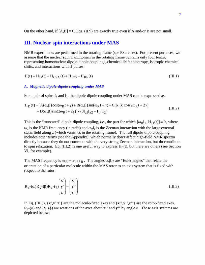
In Eq. (III.3), {x’,y’,z’} are the molecule-fixed axes and {x’’,y’’,z’’} are the rotor-fixed axes. Rz’’(φ) and Ry’’(φ) are rotations of the axes about z’’ and y’’ by angle φ. These axis systems are depicted below:

8
Schematic depiction of an MAS rotor, showing rotor-fixed axes {x’’,y’’,z’’} and randomly oriented molecules with molecule-fixed axes {x’,y’,z’}. The two axis systems are related by rotations by Euler angles, as in Eq. (III.3), which are different for different molecules. The MAS rotor rotates about its z’’ axis. The coefficients A(α,β), B(α,β), C(α,β), and D(α,β) in Eq. (III.2) are proportional to γI
2/R3, where γI is the gyromagnetic ratio and R is the internuclear distance. We shall not worry about the detailed functional form of these coefficients in the analyses of recoupling sequences presented below. See the Appendix for a complete derivation of Eq. (III.2), including general expressions for these coefficients. The maximum value of the total coefficient of
)II3( 212z1z II ⋅− is 32I R/hγ . For 13C spin pairs, this is 2π×7.59 kHz when R = 1.00 Å.
Note that the dependence on the Euler angle γ always appears as ωRt + γ. This is because molecules with different values of γ (but the same α and β) differ in their orientations by a rotation about z'', which is the MAS rotation axis. So, as the sample spins, molecules with different values of γ are rotated into one another, thus having the same coefficient of
)II3( 212z1z II ⋅− at different values of t. Note that the time average of HD(t) is zero under MAS. Note also that HD(t) contains terms that oscillate at ωR and terms that oscillate at 2ωR. Finally, note that HD(t) is a “zero-quantum operator”. This means that HD(t) has non-zero matrix elements only between states that have the same total z component of angular momentum. For a system of two spin-1/2 nuclei, the only non-zero matrix elements are
2/1|)II3(||)II3(| 212z1z212z1z =>−−⋅−−−<=>++⋅−++< IIII (III.4a)

9
2/1|)II3(||)II3(| 212z1z212z1z −=>+−⋅−−+<=>−+⋅−+−< IIII (III.4b) The dipole-dipole coupling for a static sample is obtained by setting ωR to zero in Eq. (III.2). Recoupled dipole-dipole interactions generally have different orientation dependences than static couplings (i.e., different dependences on α,β,γ), and can be zero-quantum, one-quantum, or two-quantum operators (or a mixture of these). B. Chemical shift anisotropy and isotropic chemical shift For one spin I,
zRR
RRCSAI)]2t2sin(),('D)2t2cos(),('C
)tsin(),('B)tcos(),('A[)t(Hγ+ωβα+γ+ωβα+
γ+ωβα+γ+ωβα= (III.5a)
zIICS IH ω= (III.5b) The isotropic chemical shift ωI is defined here to be the time-independent part of the difference between the actual NMR frequency of spin I and the rf carrier frequency ωrf. Under MAS, the chemical shift anisotropy (CSA) has the same type of time-dependence as the dipole-dipole coupling (i.e., terms that oscillate at ωR and 2ωR), but the operator part is simply Iz. An important difference is that
)t(He)t(He DiI
DiI xx =ππ− (III.6a)
but
)t(He)t(He CSAiI
CSAiI xx −=ππ− (III.6b)
This allows chemical shifts and dipole-dipole couplings to be affected differently by pulse sequences, especially recoupling sequences. C. Radio-frequency pulses
)]t(sinI)t(cosI)[t()t(H yx1RF φ+φω= (III.7) The rf amplitude is ω1(t). The rf phase is φ(t). When a pulse sequence contains short pulses with amplitudes that greatly exceed the strengths of dipole-dipole and chemical shift interactions and the MAS frequency, the pulses can be treated as instantaneous rotations of spin angular momenta. This is the delta-function pulse limit. In this limit, the rotation (i.e., the evolution operator) produced by a pulse of length tp is the operator
10
)(R)(R)(R)(Re)(R
e),(R
zxz
ziI
z
)sinIcosI(i
x
yx
φ−θφ=φ−φ=
=φθθ−
θφ+φ−
(III.7)
where θ = ω1tp is the pulse flip angle. In general, the net rotation produced by a pulse sequence alone (i.e., ignoring HD(t), HCSA(t), and HICS) is
∫ φ+φω−=t0 yx1RF )]}'t(sinI)'t(cosI)['t('dtiexp{T)t(U
r (III.8)
If all pulses in a pulse sequence are phase-shifted by Δφ, then the net rotation becomes
φΔφΔ−
φΔφΔ−
φΔφΔ−
=
φ+φω−=
φ+φω−=
φΔ+φ+φΔ+φω−=φΔ
∫
∫
∫
zz
zz
zz
iIRF
iI
iIt0 yx1
iI
iIt0 yx1
iI
t0 yx1RF
e)0;t(Ue
e)]}'t(sinI)'t(cosI)['t('dtiexp{Te
]}e)]'t(sinI)'t(cosI)['t('dte[iexp{T
)]})'t(sin(I))'t(cos(I)['t('dtiexp{T);t(U
r
r
r
(III.9)
Similarly, if we include all four Hamiltonian terms, the evolution operator for the pulse sequence is
∫ +++φ+φω−=t0 ICSCSADyx1 ]}H)'t(H)'t(H)]'t(sinI)'t(cosI)['t(['dtiexp{T)t(U
r (III.10)
and a phase shift changes the evolution operator to
φΔφΔ−
φΔφΔ−
=
+++φ+φω−=
+++φΔ+φ+φΔ+φω−=φΔ
∫
∫
zz
zz
iIiI
iIt0 ICSCSADyx1
iI
t0 ICSCSADyx1
e)0;t(Ue
]}e]H)'t(H)'t(H)]'t(sinI)'t(cosI)['t(['dte[iexp{T
]}H)'t(H)'t(H)])'t(sin(I))'t(cos(I)['t(['dtiexp{T);t(Ur
r
(III.11) Eq. (III.11) is valid because HD(t), HCSA(t), and HICS all commute with Iz. If this were not true (i.e., if we were not in the high-field limit), the effect of an overall rf phase shift could be more complicated. Another useful operation is an rf phase reversal, meaning φ(t) → -φ(t). The effect of a phase reversal is to change the evolution operator to
11
xx
xx
xx
IiIi
Iit0 ICSCSADyx1
Ii
t0 ICSCSAD
Iiyx1
Ii
t0 ICSCSADyx1
t0 ICSCSADyx1
e)t(''Ue
e]]H)'t(H)'t(H)]'t(sinI)'t(cosI)['t([[e'dtiexp{T
]H)'t(H)'t(He)]'t(sinI)'t(cosI)['t([e'dtiexp{T
]H)'t(H)'t(H)]'t(sinI)'t(cosI)['t(['dtiexp{T
]H)'t(H)'t(H))]'t(sin(I))'t(cos(I)['t(['dtiexp{T)t('U
ππ−
ππ−
ππ−
=
−−+φ+φω−=
+++φ+φω−=
+++φ−φω−=
+++φ−+φ−ω−=
∫
∫
∫
∫
r
r
r
r
(III.12) Thus, a phase reversal is equivalent to changing the sign of chemical shifts and rotating the resulting evolution operator U’’(t) by 180° around x. IV. Average Hamiltonian Theory in simple terms AHT [Haeberlen and Waugh, Phys. Rev. 175, 453 (1968)] is a mathematical formalism that allows us to analyze how pulse sequences affect internal spin interactions1,2. AHT is particularly useful in the derivation and analysis of pulse sequences that consist of a block of rf irradiation that is repeated many times. This is precisely the situation that arises in dipolar recoupling experiments. If the rf block has length τc (called the cycle time), then AHT is applicable when the following conditions are met:
)t(H)t(H RFcRF =+τ (IV.1a) )t(H)t(H DcD =+τ (IV.1b)
)t(H)t(H CSAcCSA =+τ (IV.1c)
1)(U cRF =τ (IV.2)
1||H||,1||H||,1||H|| cICScCSAcD <<τ<<τ<<τ (IV.3) Eqs. (IV.1) says that the rf pulse sequence is periodic and the internal spin interactions are also periodic. In recoupling sequences, this means τc should be a multiple of τR. Eq. (IV.2) says that the net rotation produced by the rf block is zero (or sometimes a multiple of 2π). The rf block is then called a “cycle”. Eq. (IV.3) says that τc is short enough that the dipole-dipole and chemical shift interactions can not produce a large change in the state of the spin system in one cycle. This allows a “perturbation theory” approach such as AHT to be employed, based on Eq. (II.9). AHT depends on changing the picture in which we view the evolution of the spin system from the usual rotating frame (in which HRF, HD, HCSA, and HICS together determine the spin evolution) to a new frame of reference in which the rf pulses no longer appear directly. Instead,
12
the rf pulses cause additional time dependences in HD, HCSA, and HICS. This new frame of reference is called the interaction representation with respect to HRF. Mathematically, the interaction representation works as follows: If U(t) is the evolution operator for the entire rotating frame Hamiltonian, we define a new evolution operator )t(U~ that satisfies
)t(U~)t(U)t(U RF= . Then we ask, “What is the new Hamiltonian that corresponds to )t(U~ ?”
This is easily calculated, using the general relations )t(U)t(H)t(Udtdi = [see Eq. (I.4)] and
)t(H)t(U])t(U[dtdi 11 −− −= [see Eqs (II.8) and recall that U(t) is unitary and H(t) is Hermitean;
also, the adjoint of the number i is –i].
)t(U~)t(U]H)t(H)t(H[)t(U
)t(U]H)t(H)t(H)t(H[)t(U)t(U)t(H)t(U
)t(Udtdi)t(U)t(U])t(U[
dtdi
)]t(U)t(U[dtdi)t(U~
dtdi
RFICSCSAD1
RF
ICSCSADRF1
RFRF1
RF
1RF
1RF
1RF
++=
++++−=
⎟⎠⎞
⎜⎝⎛+⎟
⎠⎞
⎜⎝⎛=
=
−
−−
−−
−
(IV.4)
Therefore,
ICSCSAD H~)t(H~)t(H~)t(H~ ++= (IV.5) with
)t(U)t(H)t(U)t(H~ RFD1
RFD−= (IV.6a)
)t(U)t(H)t(U)t(H~ RFCSA1
RFCSA−= (IV.6b)
)t(UH)t(UH~ RFICS1
RFICS−= (IV.6c)
So the dipole-dipole and chemical shift Hamiltonian terms in the interaction representation are the same as in the usual rotating frame, but with their spin operator parts rotated by 1
RF )t(U − . (Note that this rotation is the inverse of )t(URF , so the order of the pulses in a pulse sequence is reversed and the sign of the flip angles is changed. This is very important in AHT calculations.)
1RF )t(U − acts on the spin operator parts of HD(t), HCSA(t), and HICS(t), making these spin
operator parts time-independent. In recoupling techniques, the time-dependence of the spin operator parts induced by the rf pulses interferes with the spatial time dependence from MAS, in general preventing )t(H~ D and/or )t(H~ CSA from averaging to zero.

13
Because of Eq. (IV.2), )(U~)(U cc τ=τ . Because of Eq. (IV.1), Ncc )(U~)N(U τ=τ . Because of
Eq. (IV.3), we can approximate )(U~ cτ by
cave
c
H~i0c
e
})t(H~dtiexp{)(U~
τ−
τ
=
−≈τ ∫ (IV.7)
with ∫τ
τ= c
0cave )t(H~dt1H~ . Therefore, as long as we care only about the state of the spin system
at multiples of τc (and not in the middle of the rf blocks), then it is sufficient to calculate the average Hamiltonian in the interaction representation. To a good approximation, the NMR signals will be determined by aveH~ alone. V. Homonuclear dipolar recoupling mechanisms A. Delta-function pulse sequences Consider the following simple pulse sequence, called DRAMA [see R. Tycko and G. Dabbagh, Chem. Phys. Lett. 173, 461 (1990)]3:
How do we use AHT to calculate what this does to homonuclear dipole-dipole couplings and chemical shifts? Because the sequence consists of delta-function pulses, )t(URF is piecewise-constant:
⎪⎩
⎪⎨
⎧
τ<<ττ<<τ
τ<<= π−
R2
212/iI
1
RFt,1
t,et0,1
)t(U x (V.1)
Abbreviating )2t2sin(D)2t2cos(C)tsin(B)tcos(A RRRR γ+ω+γ+ω+γ+ω+γ+ω from Eq. (III.2) by (A,B,C,D), the interaction representation Hamiltonians are

14
⎪⎩
⎪⎨
⎧
τ<<τ⋅−×τ<<τ⋅−×τ<<⋅−×
=
R2212z1z
21212y1y
1212z1z
Dt),II3()D,C,B,A(t),II3()D,C,B,A(t0),II3()D,C,B,A(
)t(H~
IIIIII
(V.2)
⎪⎩
⎪⎨
⎧
τ<<τ×τ<<τ×τ<<×
=
R2z
21y
1z
CSAt,I)'D,'C,'B,'A(t,I)'D,'C,'B,'A(t0,I)'D,'C,'B,'A(
)t(H~ (V.3a)
⎪⎩
⎪⎨
⎧
τ<<τωτ<<τωτ<<ω
=
R2zI
21yI
1zI
ICSt,It,It0,I
)t(H~ (V.3b)
The average Hamiltonians are
)]}22cos()22[cos(4D)]22sin()22[sin(
4C
)]cos()[cos(2B)]sin()[sin(
2A){IIII(3H~
1R2R1R2R
1R2R1R2R2z1z2y1yave,D
γ+τω−γ+τωπ
−γ+τω−γ+τωπ
+
γ+τω−γ+τωπ
−γ+τω−γ+τωπ
−=
(V.4)
)]}22cos()22[cos(4
'D)]22sin()22[sin(4
'C
)]cos()[cos(2
'B)]sin()[sin(2
'A){II(H~
1R2R1R2R
1R2R1R2Rzyave,CSA
γ+τω−γ+τωπ
−γ+τω−γ+τωπ
+
γ+τω−γ+τωπ
−γ+τω−γ+τωπ
−=
(V.5a)
]I)II[(H~ zR
12zyIave,ICS +
ττ−τ
−ω= (V.5b)
So both the dipole-dipole coupling and the CSA are recoupled, and the isotropic chemical shift is altered. Note that only the 2z1z II3 part of HD(t) contributes to the recoupled dipole-dipole Hamiltonian. This is a general rule, because the I1⋅I2 part is not affected by the rf pulses. Now consider a longer DRAMA pulse sequence with additional 180° pulses:

15
For this sequence
⎪⎪⎪⎪
⎩
⎪⎪⎪⎪
⎨
⎧
τ<<τ+ττ+τ<<τ+τ
τ+τ<<ττ<<τ
τ<<ττ<<
=
π−
π−
π−
π−
R2RiI
2R1R2/3iI
1RRiI
R2
212/iI
1
RF
2t,et,e
t,et,1
t,et0,1
)t(U
x
x
x
x
(V.6)
⎪⎪⎪⎪
⎩
⎪⎪⎪⎪
⎨
⎧
τ<<τ+τ⋅−×τ+τ<<τ+τ⋅−×
τ+τ<<τ⋅−×τ<<τ⋅−×τ<<τ⋅−×τ<<⋅−×
=
R2R212z1z
2R1R212y1y
1RR212z1z
R2212z1z
21212y1y
1212z1z
D
2t),II3()D,C,B,A(t),II3()D,C,B,A(
t),II3()D,C,B,A(t),II3()D,C,B,A(t),II3()D,C,B,A(t0),II3()D,C,B,A(
)t(H~
IIII
IIIIIIII
(V.7)
⎪⎪⎪⎪
⎩
⎪⎪⎪⎪
⎨
⎧
τ<<τ+τ×−τ+τ<<τ+τ×−
τ+τ<<τ×−τ<<τ×τ<<τ×τ<<×
=
R2Rz
2R1Ry
1RRz
R2z
21y
1z
CSA
2t,I)'D,'C,'B,'A(t,I)'D,'C,'B,'A(
t,I)'D,'C,'B,'A(t,I)'D,'C,'B,'A(t,I)'D,'C,'B,'A(t0,I)'D,'C,'B,'A(
)t(H~ (V.8a)
⎪⎪⎪⎪
⎩
⎪⎪⎪⎪
⎨
⎧
τ<<τ+τω−τ+τ<<τ+τω−
τ+τ<<τω−τ<<τωτ<<τωτ<<ω
=
R2RzI
2R1RyI
1RRzI
R2zI
21yI
1zI
ICS
2t,It,I
t,It,It,It0,I
)t(H~ (V.8b)
16
Now, ave,DH~ is the same as before (because )t(H~ D is not affected by the additional 180°
pulses), but 0H~H~ ave,ICSave,CSA == (because the 180° pulses change the signs of )t(H~ CSA
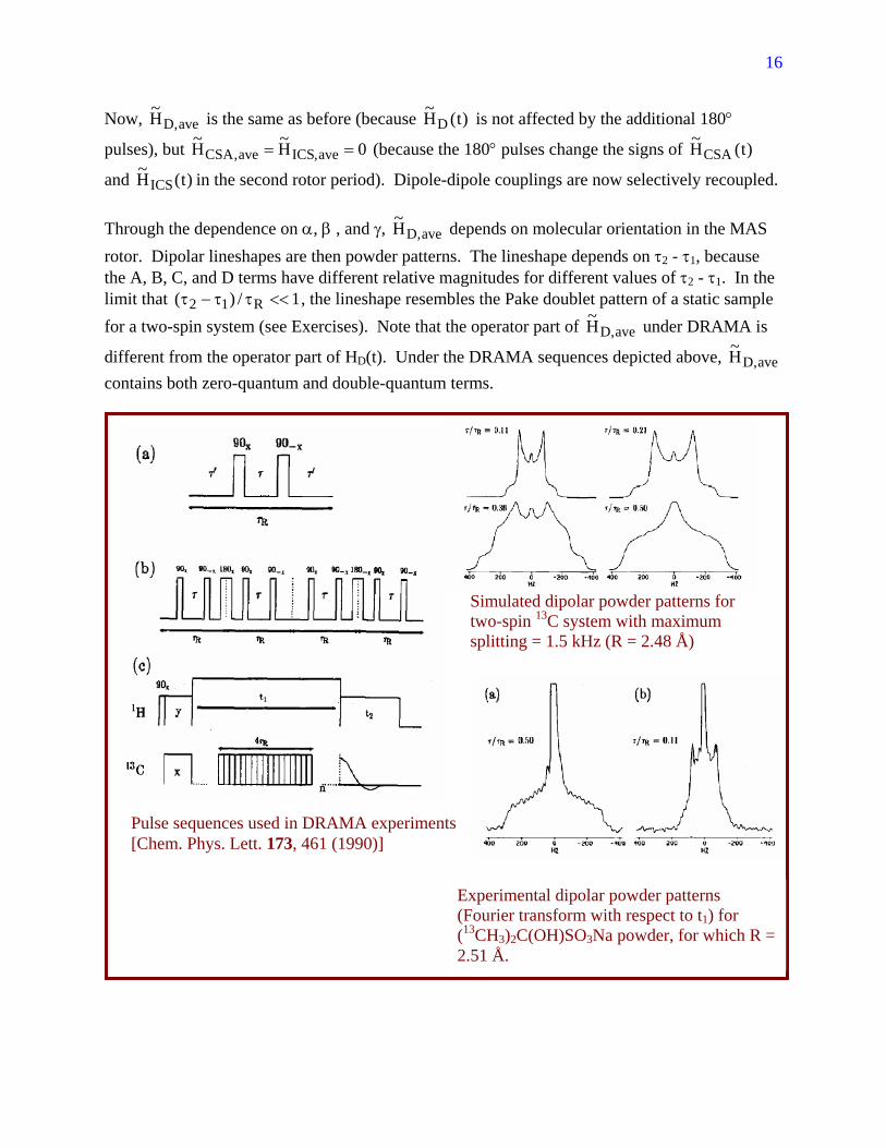
and )t(H~ ICS in the second rotor period). Dipole-dipole couplings are now selectively recoupled. Through the dependence on α, β , and γ, ave,DH~ depends on molecular orientation in the MAS rotor. Dipolar lineshapes are then powder patterns. The lineshape depends on τ2 - τ1, because the A, B, C, and D terms have different relative magnitudes for different values of τ2 - τ1. In the limit that 1/)( R12 <<ττ−τ , the lineshape resembles the Pake doublet pattern of a static sample for a two-spin system (see Exercises). Note that the operator part of ave,DH~ under DRAMA is
different from the operator part of HD(t). Under the DRAMA sequences depicted above, ave,DH~ contains both zero-quantum and double-quantum terms.
Simulated dipolar powder patterns for two-spin 13C system with maximum splitting = 1.5 kHz (R = 2.48 Å)
Pulse sequences used in DRAMA experiments [Chem. Phys. Lett. 173, 461 (1990)]
Experimental dipolar powder patterns (Fourier transform with respect to t1) for (13CH3)2C(OH)SO3Na powder, for which R = 2.51 Å.

17
B. Continuous rf irradiation Consider the following pulse sequence, called 2Q-HORROR [see N.C. Nielsen, H. Bildsoe, H.J. Jakobsen, and M.H. Levitt, J. Chem. Phys. 101, 1805 (1994)]4:
In other words, the cycle here is a 90y-360x-90-y sequence, with delta-function 90° pulses and a very long, weak 360° pulse. For this sequence,
2/iI2/tiI
2/iItiIRF
yRx
y1x
ee
ee)t(Uπ−ω−
π−ω−
=
= (V.9)
for 0 < t < 2τR. The interaction representation Hamiltonians are then
]))IIII(tsin)IIII(itcos)IIII((43[)D,C,B,A(
])tsin)IIII()IIII(tcos)IIII((23[)D,C,B,A(
]2
tcos2
tsin)IIII(2
tsinII2
tcosII(3[)D,C,B,A(
])2
tsinI2
tcosI)(2
tsinI2
tcosI(3[)D,C,B,A()t(H~
212121R2121R2121
21R2y1x2x1y2y1y2x1xR2y1y2x1x
21RR
2y1x2x1yR2
2y1yR2
2x1x
21R
2yR
2xR
1yR
1xD
II
II
II
II
⋅−++ω−+ω+×=
⋅−ω+−++ω−×=
⋅−ωω
+−ω
+ω
×=
⋅−ω
+ω
−ω
+ω
−×=
+−−+−−++−−++
(V.10)
)2
tsinI
2t
cosI()'D,'C,'B,'A()t(H~ Ry
RxCSA
ω+
ω−×= (V.11a)
)2
tsinI
2t
cosI()t(H~ Ry
RxIICS
ω+
ω−ω= (V.11b)
Eq. (V.10) makes use of the identities 2/)2cos1(cos2 θ+=θ and 2/)2cos1(sin2 θ−=θ , as well as I± = Ix + iIy. Although )t(H~ D contains both double-quantum and zero-quantum operator terms, only the double-quantum terms oscillate in time. Therefore, only the double-quantum
terms are recoupled. Using the relations ∫τ
δτ=ωωR2
0 n,kRRR
2tncos
2tkcosdt ,

18
∫τ
δτ=ωωR2
0 n,kRRR
2tnsin
2tksindt , and ∫
τ=
ωωR20
RR 02
tncos2
tksindt for integers k and n, it
is straightforward to show that 0H~H~ ave,ICSave,CSA == and that
)]cosBsinA)(IIII(i)sinBcosA)(IIII[(83H~ 21212121ave,D γ+γ−−+γ+γ+= −−++−−++ (V.12)
Thus, the 2Q-HORROR sequence creates a pure double-quantum recoupled Hamiltonian (assuming that the AHT approximation is valid and that the pulses are perfect). The average Hamiltonian contains two double-quantum terms, whose magnitudes depend on the Euler angles α,β,γ. Interestingly, the overall magnitude of ave,DH~ is independent of the γ angle (see Exercises). Recoupling sequences with this property are called “γ-encoded”. This property causes the dipolar powder pattern lineshape under 2Q-HORROR and other γ-encoded sequences to have two sharp horns (see below), which means that the signal decay under ave,DH~ is strongly oscillatory. This is good for quantitative measurements of internuclear distances, and also for double-quantum filtering efficiencies.
Simulated and experimental 2Q-HORROR data for a 13C-13C pair with R ≈ 1.54 Å [from Nielsen et al, J. Chem. Phys. 101, 1805 (1994)].

19
C. Finite-pulse recoupling sequences Consider the following sequence, called “finite-pulse Radio-Frequency-Driven Recoupling” or fpRFDR [see Y. Ishii, J. Chem. Phys. 114, 8473 (2001) and A.E. Bennett, C.M. Rienstra, J.M. Griffiths, W.G. Zhen, P.T. Lansbury, and R.G. Griffin, J. Chem. Phys. 108, 9463 (1998)]5,6:
The cycle time is 4τR, there is one 180° pulse in each rotor period, and the pulse length is a significant fraction of the rotor period. The rf amplitude during each pulse is
p1 τ
π=ω . For this
pulse sequence,
⎪⎪⎪⎪⎪⎪⎪
⎩
⎪⎪⎪⎪⎪⎪⎪
⎨
⎧
τ<<τ+τ
τ+τ<<τ
τ<<τ+τ
τ+τ<<τ
τ<<τ+τ
τ+τ<<τ
τ<<τ
τ<<
=
π−π−π−π−
π−π−π−ττ−π−
π−π−π−
π−π−ττ−π−
π−π−
π−ττ−π−
π−
τπ−
RpRIiIiIiIi
pRRIiIiIi/)3t(Ii
RpRIiIiIi
pRRIiIi/)2t(Ii
RpRIiIi
pRRIi/)t(Ii
RpIi
p/tIi
RF
4t3,eeee
3t3,eeee
3t2,eee
2t2,eee
2t,ee
t,ee
t,e
t0,e
)t(U
xyxy
xyxpRy
xyx
xypRx
xy
xpRy
x
px
(V.13)
Using the identity zxy IiIiIi eee ππ−π− = (see Exercises), Eq. (V.13) can be simplified:

20
⎪⎪⎪⎪⎪⎪
⎩
⎪⎪⎪⎪⎪⎪
⎨
⎧
τ<<τ+ττ+τ<<τ
τ<<τ+τ
τ+τ<<τ
τ<<τ+τ
τ+τ<<τ
τ<<τ
τ<<
=
ππ−ττ−π−
ππ−
πττ−π−
π
π−ττ−π−
π−
τπ−
RpR
pRRIiIi/)2t(Ii
RpRIiIi
pRRIi/)2t(Ii
RpRIi
pRRIi/)t(Ii
RpIi
p/tIi
RF
4t3,13t3,eee
3t2,ee
2t2,ee
2t,e
t,ee
t,e
t0,e
)t(U
zxpRy
zx
zpRx
z
xpRy
x
px
(V.14)
Ignoring the I1⋅I2 term (which is not recoupled, as explained above), the interaction-representation dipole-dipole Hamiltonian is then
⎪⎪⎪⎪⎪⎪⎪⎪
⎩
⎪⎪⎪⎪⎪⎪⎪⎪
⎨
⎧
τ<<τ+τ×
τ+τ<<ττ
τ−π−
τ
τ−π
τ
τ−π−
τ
τ−π×
τ<<τ+τ×
τ+τ<<τττ−π
−ττ−π
ττ−π
−ττ−π
×
τ<<τ+τ×
τ+τ<<ττ
τ−π+
τ
τ−π
τ
τ−π+
τ
τ−π×
τ<<τ×
τ<<τπ
+τπ
τπ
+τπ
×
=
RpR2z1z
pRRp
)R2x
p
)R2z
p
)R1x
p
)R1z
RpR2z1z
pRRp
R2y
p
R2z
p
R1y
p
R1z
RpR2z1z
pRRp
)R2x
p
)R2z
p
)R1x
p
)R1z
Rp2z1z
pp
2yp
2zp
1yp
1z
D
4t3),II3()D,C,B,A(
3t3)],3t(
sinI3t(
cosI)(3t(
sinI3t(
cosI(3[)D,C,B,A(
3t2),II3()D,C,B,A(
2t2)],)2t(sinI)2t(cosI)()2t(sinI)2t(cosI(3[)D,C,B,A(
2t),II3()D,C,B,A(
t)],t(
sinIt(
cosI)(t(
sinIt(
cosI(3[)D,C,B,A(
t),II3()D,C,B,A(
t0)],tsinItcosI)(tsinItcosI(3[)D,C,B,A(
)t(H~
(V.15a) This can be rewritten as
⎪⎪⎪⎪⎪⎪⎪⎪
⎩
⎪⎪⎪⎪⎪⎪⎪⎪
⎨
⎧
τ<<τ+τ×
τ+τ<<τττ−π
ττ−π
+−ττ−π
+ττ−π
×
τ<<τ+τ×
τ+τ<<ττ
τ−πτ
τ−π+−
ττ−π
+τ
τ−π×
τ<<τ+τ×
τ+τ<<τττ−π
ττ−π
++ττ−π
+ττ−π
×
τ<<τ×
τ<<τπ
τπ
++τπ
+τπ
×
=
RpR2z1z
pRRp
R
p
R2z1x2x1z
p
R22x1x
p
R22z1z
RpR2z1z
pRRp
R
p
R2z1y2y1z
p
R22y1y
p
R22z1z
RpR2z1z
pRRp
R
p
R2z1x2x1z
p
R22x1x
p
R22z1z
Rp2z1z
ppp
2z1y2y1zp
22y1y
p
22z1z
D
4t3),II3()D,C,B,A(
3t3)],)3t(
cos)3t(
sin)IIII()3t(
sinII)3t(
cosII(3[)D,C,B,A(
3t2),II3()D,C,B,A(
2t2)],)2t(
cos)2t(
sin)IIII()2t(
sinII)2t(
cosII(3[)D,C,B,A(
2t),II3()D,C,B,A(
t)],)t(
cos)t(
sin)IIII()t(
sinII)t(
cosII(3[)D,C,B,A(
t),II3()D,C,B,A(
t0)],tcostsin)IIII(tsinIItcosII(3[)D,C,B,A(
)t(H~
(V.15b) Note that the signs of Iz1Ix2+Ix1Iz2 and Iz1Iy2+Iy1Iz2 are reversed in the third and fourth rotor periods, relative to the first and second rotor periods. This is a consequence of the choice of

21
phases in the fpRFDR sequence [called XY-4 phases7], and it causes these single-quantum terms to cancel out in the average Hamiltonian. Evaluating the integrals in the average Hamiltonian, we find (omitting many intermediate steps)
]II3[
}D]2cos)22[cos()(16
)(3C]2sin)22[sin()(16
)(3
B]cos)[cos()4(16
)4(3A]sin)[sin()4(16
)4(3{
)]IIII(21II[
}D]2cos)22[cos()(8
)(3C]2sin)22[sin()(8
)(3
B]cos)[cos()4(8
)4(3A]sin)[sin()4(8
)4(3{
}tsin)II3II3()D,C,B,A(dt2
)tcosII3()D,C,B,A(dt4)II3()D,C,B,A(dt4{4
1
})t(H~dt)t(H~dt)t(H~dt)t(H~dt)t(H~dt4{4
1H~
212z1z
pR21
2R
21
2R
pR21
2R
21
2R
pR21
2R
21
2R
pR21
2R
21
2R
2y1y2x1x2z1z
pR21
2R
21
2R
pR21
2R
21
2R
pR21
2R
21
2R
pR21
2R
21
2R
0 p
22y1y2x1x
0 p
22z1z2z1z
R
33 D
22 DD0 DD
Rave,D
p
pR
p
pR
R
pR
R
pR
R
pR
p
II ⋅−×
γ−γ+τωω−ωπ
ω+ω−γ−γ+τω
ω−ωπ
ω+ω+
γ−γ+τωω−ωπ
ω+ω−γ−γ+τω
ω−ωπ
ω+ω=
+−×
γ−γ+τωω−ωπ
ω+ω−γ−γ+τω
ω−ωπ
ω+ω+
γ−γ+τωω−ωπ
ω+ω−γ−γ+τω
ω−ωπ
ω+ω=
τπ
+×+
τπ
×+×τ
=
++++τ
=
∫
∫∫
∫∫∫∫∫
τ
ττ
τ
τ+τ
τ
τ+τ
τ
τ+τ
τ
ττ
τ
(V.16) Miraculously (or as a consequence of symmetry, as described below), the average dipole-dipole Hamiltonian under the fpRFDR sequence is a zero-quantum operator with the same operator form as the dipole-dipole coupling in a non-spinning sample. This has useful consequences in certain applications, for example by allowing ideas that were originally developed for NMR of static solids to be applied in MAS experiments8,9. Under fpRFDR, it is also true that 0H~H~ ave,ICSave,CSA == (see Exercises). ω1 in Eq. (V.16) is the rf amplitude during the 180° pulses. Note that ave,DH~ vanishes as
∞→ω1 and 0p →τ (i.e., in the delta-function pulse limit). As shown below, a different recoupling mechanism, leading to a different average dipole-dipole Hamiltonian, comes into play when the coupled spins have large chemical shift differences. This chemical-shift-driven recoupling mechanism does not disappear in the delta-function pulse limit.

22
D. Chemical-shift-driven recoupling 1. Rotational resonance Now consider the case where two dipole-coupled spins have a large difference in their isotropic chemical shifts. Ignore chemical shift anisotropy for now. The nuclear spin Hamiltonian under MAS is then
)t(H)II()II(
)t(H)II)(()II)((
)t(HII)t(H
D2z1z21
2z1z21
D2z1z2I1I21
2z1z2I1I21
D2z2I1z1I
+−Δ++Σ=
+−ω−ω++ω+ω=
+ω+ω=
(V.17)
where Σ and Δ are the sum and difference of the two chemical shifts (actually, resonance offsets). Now go into an interaction representation with respect to the chemical shift terms. If U(t) is the evolution operator for H(t), this interaction representation is defined by
)t(U~)t(U)t(U ICS= (V.18a)
]t)II(exp[]t)II(exp[
}t)]II()II([iexp{)t(U
2z1z2i
2z1z2i
2z1z21
2z1z21
ICS
−Δ−+Σ−=
−Δ++Σ−= (V.18b)
})'t(H~'dtiexp{T)t(U~t0 D∫−=
r (V.18c)
]t)II(exp[)]IIII](t)II(exp[)D,C,B,A(
)II2()D,C,B,A(
]t)II(exp[)]IIII(II2][t)II(exp[)D,C,B,A(
]t)II(exp[)II3](t)II(exp[)D,C,B,A(
]t)II(exp[)t(H]t)II(exp[
)t(U)t(H)t(U)t(H~
2z1z2i
21212z1z2i
21
2z1z
2z1z2i
212121
2z1z2z1z2i
2z1z2i
212z1z2z1z2i
2z1z2i
D2z1z2i
ICSD1
ICSD
−Δ−+−Δ×−
×=
−Δ−+−−Δ×=
−Δ−⋅−−Δ×=
−Δ−−Δ=
=
+−−+
+−−+
−
II
(V.19) Eq. (V.19) uses the facts that [(Iz1+Iz2),HD(t)] = 0, so the Σ part of the chemical shift does not affect )t(H~ D , and that [(Iz1-Iz2),Iz1Iz2] = 0, so the Iz1Iz2 part of HD(t) is not affected by the
chemical shifts. Also, Eq. (V.19) uses the identity )IIII(II 212121
2z1z21 +−−+ ++=⋅ II . Now,
using the identity ±φ±φ−
±φ = IeeIe iiIiI zz , Eq. (V.19) becomes
]II)tsinit(cosII)tsinit[(cos)D,C,B,A()II2()D,C,B,A(
)IIeIIe()D,C,B,A()II2()D,C,B,A()t(H~
212121
2z1z
21ti
21ti
21
2z1zD
+−−+
+−Δ−
−+Δ
Δ−Δ+Δ+Δ×−×=
+×−×=

23
(V.20) Eq. (V.20) shows that the Iz1Iz2 part of the dipole-dipole coupling is not recoupled by the chemical shift difference, but the “flip-flop” part can be recoupled if R|| ω=Δ or R2|| ω=Δ . These are the “n = 1” and “n = 2” rotational resonance conditions10-14. At the rotational resonance conditions, )t(H~ D is periodic with period τR and AHT can be applied. The average dipole-dipole Hamiltonian at rotational resonance is
21n,2i2
n,1i
41
21n,2i2
n,1i
41
ave,D II]e)iDC(e)iBA[(II]e)iDC(e)iBA[(H~ +−γγ
−+γ−γ− δ−+δ−−δ++δ+−=
(V.21) for n = 1 or n = 2. Note that this is a zero-quantum operator, but it is not the same as the zero-quantum operator created by the fpRFDR sequence. In a system with many 13C-labeled sites, rotational resonance allows pairs of spins with particular chemical shift differences to be recoupled selectively15,16, as shown below. However, unless the MAS frequency is varied during the pulse sequence, the couplings can not be switched on and off. Therefore, other approaches to frequency-selective homonuclear dipolar recoupling that employ rf pulses and do not depend on being exactly on rotational resonance have been developed by several groups17-22.
13C NMR spectra of U-15N,13C-alanine powder, recorded at 100.8 MHz, with MAS frequencies indicated by dashed lines. At the rotational resonance conditions, the recoupled lines become dipolar powder patterns, while other lines remain sharp. Close to rotational resonance conditions (C and D), the main NMR lines of strongly coupled pairs exhibit apparent shifts on the order of 0.5 ppm, which can complicate accurate measurements of chemical shifts in uniformly labeled samples.

24
2. Radio-Frequency-Driven Recoupling Consider the Hamiltonian in Eq. (V.17), but with an additional HRF(t) term that corresponds to the following pulse sequence, with m being an arbitrary positive integer:
This sequence, called SEDRA23 or more commonly RFDR6,24, can be analyzed by first transforming the Hamiltonian into an interaction representation with respect to HRF(t), and then into an interaction representation with respect to the chemical shifts. Following the same principles as used above for other recoupling sequences, the Hamiltonian in the interaction representation with respect to HRF(t) is
⎪⎪⎩
⎪⎪⎨
⎧
τ<<τ+−Δ++Σ
τ<<τ+−Δ−+Σ−
τ<<+−Δ++Σ
=
ccD2z1z21
2z1z21
ccD2z1z21
2z1z21
cD2z1z21
2z1z21
t4/3),t(H)II()II(
4/3t4/),t(H)II()II(
4/t0),t(H)II()II(
)t(H~ (V.21)
HD(t) is not affected directly by the delta-function 180° pulses, but the chemical shifts change sign between the two 180° pulses. Therefore, the isotropic chemical shifts now appear to be time-dependent. In the second interaction representation, the dipole-dipole coupling becomes
⎪⎪⎩
⎪⎪⎨
⎧
τ<<ττ−−Δ−τ−−Δ
τ<<τ−τ
−Δ−−τ
−Δ
τ<<−Δ−−Δ
=
ccc2z1z2i
Dc2z1z2i
ccc
2z1z2i
Dc
2z1z2i
c2z1z2i
D2z1z2i
D
t4/3)],t)(II(exp[)t(H)]t)(II(exp[
4/3t4/)],t2
)(II(exp[)t(H)]t2
)(II(exp[
4/t0],t)II(exp[)t(H]t)II(exp[
)t(H~~
(V.22) Ignoring the Iz1Iz2 part of HD(t), which as shown above is not recoupled, Eq. (V.22) can be written as
⎪⎪⎩
⎪⎪⎨
⎧
τ<<τ+×−
τ<<τ+×−
τ<<+×−
=
+−τ−Δ−
−+τ−Δ
+−−τΔ−
−+−τΔ
+−Δ−
−+Δ
cc21)t(i
21)t(i
21
cc21)t2/(i
21)t2/(i
21
c21ti
21ti
21
D
t4/3],IIeIIe[)D,C,B,A(
4/3t4/],IIeIIe[)D,C,B,A(
4/t0],IIeIIe[)D,C,B,A(
)t(H~~
cc
cc (V.23)

25
The average Hamiltonian is then
)IIII)](2sinD2cosC()4(m
)2/msin()sinBcosA()(m)2/msin()1[(H
~~212122
RR
R22
RR
Rmave,D +−−+ +γ+γ
Δ−ωτ
τΔΔ+γ+γ
Δ−ωτ
τΔΔ−=
(V.24) Note that the average dipole-dipole Hamiltonian, evaluated in the double interaction representation described above, is non-zero for nearly all values of the chemical shift difference
Δ. This is because the 180° pulses, spaced mτR apart, force the flip-flop term in )t(H~~
D to be
periodic with period 2mτR. For nearly all values of Δ, )t(H~~
D has non-zero Fourier components
at ωR and/or 2ωR. However, 0H~~
ave,D → as 0→Δ . Thus, the recoupling mechanism for RFDR in the delta-function pulse limit (i.e., when the 180° pulses are very short compared with τR) is qualitatively different from the recoupling mechanism in the finite-pulse limit (i.e., when the 180° pulses occupy a significant fraction of the rotor period). In actual experiments, the phases of the 180° pulses are usually chosen to follow an XY-4 or high XY-n phase pattern7, because XY-n phase patterns compensate for rf inhomogeneity, resonance offsets, and other imperfections in the 180° pulses. This makes the RFDR technique (and the fpRFDR version) quite robust and useful in many experimental situations. VI. Symmetry principles for recoupling sequences A. Levitt’s “C” sequences Malcolm Levitt and his colleagues have developed an approach to the development of recoupling sequences that relies on general symmetry properties of pulse sequences, which lead to “selection rules” that reveal which types of interactions can be recoupled by a sequence with a given symmetry. Sequences belonging to two distinct symmetry classes have been described. The first class includes "C" sequences, comprised of rf blocks (called C elements) that produce no net rotation of spin angular momenta25,26. The general form for a C sequence is:
In other words, the C sequence contains N repetitions of the C element, with overall rf phase shifts that increase in units of φ, and with a total cycle time of n rotor periods. The phase

26
increment satisfies N/2πν=φ . N, n, and ν are positive integers. The symmetry is represented by the symbol CNn
ν. To analyze the effect of a CNn
ν sequence with AHT, one considers a general nuclear spin Hamiltonian under MAS that is a sum of terms of the form 0
timm0m TeA)t(H R λ
ωλ = in the
rotating frame [i.e., before transforming to an interaction representation with respect to HRF(t)]. Am is a function of the Euler angles α,β,γ discussed above. m is -2, -1, 1, or 2, and λ is another positive integer. Tλ0 is the "element of an irreducible tensor operator of rank λ" that commutes with the total spin angular momentum Iz. Without going into the details of irreducible tensor operators, this means Tλ0 is an operator that is a member of a set of 2λ+1 operators {Tλμ}, with μ being an integer that satisfies -λ ≤ μ ≤ λ. For dipole-dipole couplings, λ = 2 and the relevant set of operators is
)II3(T
)IIII(T
IIT
212z1z61
20
2z121z21
12
2121
22
II ⋅−=
+=
=
±±±
±±±
m (VI.1)
Thus, T2μ is a μ-quantum operator. For isotropic and anisotropic chemical shifts, the relevant operators have λ = 1. Important properties of irreducible tensor operators include:
λμμθθ−
λμθ = TeeTe iiIiI zz (VI.2a)
μ−λλπ
λμπ− −= T)1(eTe zx iIiI (VI.2b)
μ−λμ
λμ −= T)1(T † (VI.2c) Elements of the set of operators {Tλμ} are transformed into one another by rotations of spin angular momentum (i.e., by rf pulses in NMR experiments). Therefore, in the interaction representation with respect to the first C element, the nuclear spin Hamiltonian is a sum of terms of the form λμ
ωλμλμ = Te)t(A~)t(H~ tim
mm R in the interval 0 < t < nτR/N. There are 4×(2λ+1) such terms. The interaction representation Hamiltonian for the kth C element must then be a sum of terms of the form
)eTe(e)t(A~)t(H~ )1k(iI)1k(iItimmm zzR φ−
λμφ−−ω
λμλμ = (VI.3) in the interval (k-1)nτR/N < t < knτR/N, taking into account the effect of the overall rf phase shift as in Eqs. (III.8-III.11). The average Hamiltonian for the kth C element will then be a sum of terms of the form
27
timN/n0 m
N/n)1k(im)1k(i
R
N/knN/n)1k( m
Rave,m
RrRR
r
R
e)t(A~dteenNT
)t(H~dtnN)k(H~
ωτλμ
τ−ωφ−μ−λμ
τ
τ− λμλμ
∫
∫
τ=
τ=
(VI.4)
Eq. (VI.4) makes use of Eq. (VI.2a) and the fact that )t(A~ mλμ is periodic, with period equal to
nτR/N (the length of one C element). The total average Hamiltonian, for the entire cycle time nτR, is obtained by summing over contributions from all C elements. The total average Hamiltonian will then contain 4×(2λ+1) terms of the form
∑∫
∑∫
∑ ∫
=
−μν−π−ωτλμλμ
=
τ−ωφ−μ−ωτλμλμ
=
ωτλμ
τ−ωφ−μ−λμλμ
τ=
τ=
τ=
N
1k
N/)mn)(1k(2itimN/n0 m
R
N
1k
N/n)1k(im)1k(itimN/n0 m
R
N
1k
timN/n0 m
N/n)1k(im)1k(i
Rave,m
ee)t(A~dtnNT
eee)t(A~dtnNT
}e)t(A~dtee{nNTH~
Rr
RRRr
RrRR
(VI.5)
For such a term to be non-zero, the sum over k must be non-zero. But it turns out that the following relation is always true, for any positive integer N:
⎩⎨⎧
≠=
=∑=
−π−NZq,0NZq,N
eN
1k
N/q)1k(2i (VI.6)
where Z is some other integer. So the quantity μν - mn must be zero or another integer multiple of N for the average Hamiltonian under a C sequence to contain non-zero μ-quantum terms that arise from MAS-induced oscillations at frequency mωR. This is the selection rule for CNn
ν sequences. The C7 and POST-C7 recoupling sequences27,28 are good examples. For these sequences, N = 7, n = 2, and ν = 1, which imply the selection rule that μ-2m = 0, 7, 14, etc. Thus, terms with μ = 2 and m = 1 or μ = -2 and m = -1are recoupled (corresponding to double-quantum dipolar recoupling). Terms with μ = 0 and 1 are not recoupled, corresponding to the absence of CSA recoupling and the absence of both zero-quantum and one-quantum dipolar recoupling. (Recall that m has only the values ±1 and ±2, but not 0, under MAS.) C7 and POST-C7 differ in the choice of the C element itself, which is better compensated for resonance offsets in the POST-C7 case.
28
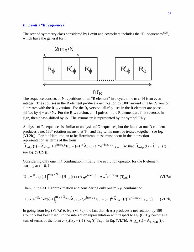
B. Levitt’s “R” sequences The second symmetry class considered by Levitt and coworkers includes the "R" sequences29,30, which have the general form
The sequence consists of N repetitions of an "R element" in a cycle time nτR. N is an even integer. The rf pulses in the R element produce a net rotation by 180° around x. The Rφ version alternates with the R’-φ version. For the Rφ version, all rf pulses in the R element are phase-shifted by N/πν=φ . For the R’-φ version, all rf pulses in the R element are first reversed in sign, then phase-shifted by -φ. The symmetry is represented by the symbol RNn
ν. Analysis of R sequences is similar to analysis of C sequences, but the fact that one R element produces a net 180° rotation means that Tλμ and Tλ-μ terms must be treated together [see Eq. (VI.2b)]. For the Hamiltonian to be Hermitean, these must occur in the interaction representation as terms of the form
μ−λω−
λμμ
λμω
λμλμ −+= Te*)t(A~)1(Te)t(A~)t(H~ timm
timmm RR [so that †
mm )t(H~)t(H~ λμλμ = ; see Eq. (VI.2c)]. Considering only one m,λ combination initially, the evolution operator for the R element, starting at t = 0, is
∫τ
λω−ω ++−=
N/n0 0
tim*m
timmRFR
R RR ]}T)eAeA()t(H[dtiexp{TUr
(VI.7a)
Then, in the AHT approximation and considering only one m,λ,μ combination,
∫τ
μ−λω−
λμμ
λμω
λμπ− −+−≈
N/n0
tim*m
timm
iIR
R RRx )]Te)t(A~)1(Te)t(A~(dtiexp[eU (VI.7b)
In going from Eq. (VI.7a) to Eq. (VI.7b), the fact that HRF(t) produces a net rotation by 180° around x has been used. In the interaction representation with respect to HRF(t), Tλ0 becomes a sum of terms of the form cλμ(t)Tλμ + (-1)μ cλμ(t)*Tλ-μ. In Eq. (VI.7b), )t(cA)t(A~ mm λμλμ ≡ .

29
Terms proportional to λμω− Te tim R and μ−λ
ω Te tim R are not shown explicitly, but of course are also present. The corresponding equations for the phase-reversed element R’, starting at t = 0, are [see Eq. (III.12)]
∫τ
λω−ωππ− ++−=
N/n0 0
tim*m
timm
iIRF
iI'R
R RRxx ]}T)eAeA(e)t(He[dtiexp{TUr
(VI.8a)
∫
∫τ
λμω−
λμμ
μ−λω
λμπ−
πτμ−λ
ω−λμ
μλμ
ωλμ
λπ−π−
−+−=
−+−−≈
N/n0
tim*m
timm
iI
iIN/n0
tim*m
timm
iIiI'R
R RRx
xR RRxx
)]Te)t(A~)1(Te)t(A~(dtiexp[e
e})]Te)t(A~)1(Te)t(A~(dt)1(iexp[e{eU (VI.8b)
Eqs. (VI.7) and (VI.8) show that UR and UR’ differ by exchange of Tλμ and Tλ-μ in the interaction representation. Including rotations about z to account for the phase shifts, the evolution operator for the first RφR’-φ pair is
∫
∫
∫
∫
∫
∫
∫
∫
∫
∫
τμ−λ
μφω−λμ
μλμ
μφ−ωλμ
τμ−λ
μφω−π−λμ
μλμ
μφ−ωπλμ
λφ
τ φμ−λ
ω−λμ
μλμ
ωλμ
φ
τμ−λ
ω−π−λμ
μλμ
ωπλμ
λφ
τ φμ−λ
ω−λμ
μλμ
ωλμ
φπ−
τλμ
ω−π−λμ
μμ−λ
ωπλμ
π−φ
τ φμ−λ
ω−λμ
μλμ
ωλμ
φπ−
τ
τ λμω−
λμμ
μ−λω
λμπ−φ
τ φμ−λ
ω−λμ
μλμ
ωλμ
π−φ−
τ
τφ−
λμω−
λμμ
μ−λω
λμπ−φ
−+−×
−+−−=
−+−×
−+−−=
−+−×
−+−=
−+−×
−+−=
−+−×
−+−=
N/n0
itimm
itimm
N/n0
i3timN/mn2im
i3timN/mn2im
iI4
N/n0
iItimm
timm
iI2
N/n0
timN/mn2im
timN/mn2im
iI
N/n0
iItimm
timm
iI2iI
N/n0
timN/mn2im
timN/mn2im
iIiI
N/n0
iItimm
timm
iI2iI
N/n2N/n
timm
timm
iIiI
N/n0
iItimm
timm
iIiI
N/n2N/n
iItimm
timm
iIiI0
R RR
R RRz
R zRRz
R RRz
R zRRzx
R RRxz
R zRRzx
R
RRRxz
R zRRxz
R
RzRRxz
]}Tee*)t(A~)1(Tee)t(A~[dtiexp{
}]Teee*)t(A~)1(Teee)t(A~[)1(dtiexp{e
e]}Te*)t(A~)1(Te)t(A~[dtiexp{e
}]Tee*)t(A~)1(Tee)t(A~[)1(dtiexp{e
e]}Te*)t(A~)1(Te)t(A~[dtiexp{ee
]}Tee*)t(A~)1(Tee)t(A~[dtiexp{ee
e]}Te*)t(A~)1(Te)t(A~[dtiexp{ee
]}Te*)t(A~)1(Te)t(A~[dtiexp{ee
e]}Te*)t(A~)1(Te)t(A~[dtiexp{ee
e]}Te*)t(A~)1(Te)t(A~[dtiexp{eeU
(VI.9) The total evolution operator is
∏−
=
φ=1)2/N(
0kR'R
NI2itotal )k(U~)k(U~eU z (VI.10)
with )k(U~ R and )k(U~ 'R defined by

30
]}Teee*)t(A~)1(
Teee)t(A~[dtiexp{)k(U~
)1k4(itimN/mnk4im
N/n0
)1k4(itimN/mnk4imR
R
R R
μ−λμφ+ω−π−
λμμ
τλμ
μφ+−ωπλμ
−+
−= ∫ (VI. 11a)
]}Teee*)t(A~)1(
Teee)t(A~[)1(dtiexp{)k(U~
)3k4(itimN/)1k2(mn2im
N/n0
)3k4(itimN/)1k2(mn2im'R
R
R R
μ−λμφ+ω−+π−
λμμ
τλμ
μφ+−ω+πλμ
λ
−+
−−= ∫ (VI.11b)
Note that 2Nφ in Eq. (VI.10) is a multiple of 2π, so the operator φzNI2ie has no effect. The average Hamiltonian for the entire R sequence is obtained by summing the exponents in UR(k) and UR’(k) over all values of k and dividing by nτR. Therefore, the coefficient of Tλμ in the average Hamiltonian arising from MAS-induced oscillations at mωR is proportional to
⎪⎪⎭
⎪⎪⎬
⎫
⎪⎪⎩
⎪⎪⎨
⎧
μν−π−=
⎪⎪⎭
⎪⎪⎬
⎫
⎪⎪⎩
⎪⎪⎨
⎧
μν−π−+μν−π=
⎪⎭
⎪⎬⎫
⎪⎩
⎪⎨⎧
+μν−π−+μν−π
∑∫
∑∑∫
∑∑∫
−
=
λπμν−τ ωλμ
−
=
λ−
=
πμν−τ ωλμ
−
=
λ−
=
πμν−τ ωλμ
]N/k)mn(2iexp[)1(e]e)t(A~[dt
]N/k)mn(2iexp[)1(]N/k)mn(2iexp[e]e)t(A~[dt
]N/)2/1k)(mn(4iexp[)1(]N/k)mn(4iexp[e]e)t(A~[dt
1N
)evenandodd(0k
kN/iN/n0
timm
1N
)odd(1k
2N
)even(0k
N/iN/n0
timm
1)2/N(
0k
1)2/N(
0k
N/iN/n0
timm
R R
R R
R R
(VI.12) Eq. (VI.12) shows that if λ is even, the coefficient of Tλμ is zero (i.e., no recoupling) unless mn - μν is an even multiple of N/2. If λ is odd, the coefficient of Tλμ is zero unless mn - μν is an odd multiple of N/2. These are the selection rules for RNn
ν sequences. Many examples of RNn
ν recoupling sequences have been reported. The fpRFDR sequence described above is a very simple example, for which n = 4, N = 4, and ν = 1. The symmetry selection rules indicate that dipole-dipole couplings (λ = 2) can be recoupled in a zero-quantum (μ = 0) form, with |m| = 1 or |m| = 2. Chemical shifts (λ = 1; |μ| = 0 or 1) can not be recoupled. This is in agreement with the detailed calculations described above. C. Cyclic time displacement symmetry and constant-time recoupling Another useful symmetry property of recoupling sequences involves their behavior when all pulses are cyclically displaced in time within the cycle time τc = nτR. In the picture below, a block of pulses (or delays) of length τ1, called P1, is displaced by τ2, causing the remaining block P2 to move from the end to the beginning of the cycle:

31
What is the effect of this cyclic displacement on a recoupled Hamiltonian? If the rotations produced by rf pulse blocks P1 and P2 are U1(t) and U2(t), with time t measured from the beginning of each block, then the total rotation before the cyclic displacement is URF(t):
⎩⎨⎧
τ<<τττ−τ<<
=R11112
11RF nt),(U)t(U
t0),t(U)t(U (VI.13)
The total rotation after the cyclic displacement is UCD(t):
⎩⎨⎧
τ<<τττ−τ<<
=R22221
22CD nt),(U)t(U
t0),t(U)t(U (VI.14)
In the interaction representation with respect to the original pulse sequence, a Hamiltonian term of the form 0
timmm TeA)t(H R λ
ωλλ = under MAS becomes (recalling that τ1 + τ2 = nτR)
⎪⎩
⎪⎨⎧
τ<<τττ<<=
⎪⎩
⎪⎨⎧
τ<<τττ−τ−ττ<<=
λ−−ωτω−
λ
λ−ω
λ
λ−−ω
λ
λ−ω
λλ
211201
21
11'timim
m
1101
1tim
m
R1111201
121
11tim
m
1101
1tim
mm
't0),(U)'t(UT)'t(U)(UeeAt0),t(UT)t(UeA
nt),(U)t(UT)t(U)(UeAt0),t(UT)t(UeA)t(H~
R1R
R
R
R
(VI.15)
with t’ = t + τ1. In the interaction representation with respect to the cyclically displaced pulse sequence, the same Hamiltonian term becomes

32
⎪⎩
⎪⎨⎧
τ<<τττ<<=
⎪⎩
⎪⎨⎧
τ<<τττ−τ−ττ<<=
λ−−ωτω−
λ
λ−ω
λ
λ−−ω
λ
λ−ω
λλ
122101
11
22''timim
m
2201
2tim
m
R2222101
211
22tim
m
2201
2tim
mm
''t0),(U)''t(UT)''t(U)(UeeAt0),t(UT)t(UeA
nt),(U)t(UT)t(U)(UeAt0),t(UT)t(UeA)t(H
R2R
R
R
R
(VI.16)
with t’’ = t + τ2. In both cases, the average Hamiltonian is the integral of the interaction representation Hamiltonian over time from 0 to nτR, divided by nτR. According to Eqs. (VI.15) and (VI.16), the integral in both cases is the sum of two integrals, over time intervals of length τ1 and τ2. Recalling that 1ee 2R1R imim =τωτω and 1)(U)(U 1122 =ττ , it can be shown that the integrands for the cyclically displaced pulse sequence are equal to the integrands for the original pulse sequence after rotation by U2(τ2)-1 = U1(τ1) and multiplication by 2Rime τω . Thus,
)(UH~)(UeH 22ave,m1
22im
ave,m 2R ττ= λ−τω
λ (VI.17) Eq. (VI.17) summarizes the effect of a cyclic time displacement on the average Hamiltonian for an arbitrary recoupling sequence. Why is this useful? As an example, consider a general recoupling sequence that ends in two periods of length τR/3. During these final two periods, either no pulses are applied or the applied pulses produce a net rotation of 2π. For such a sequence, two successive cyclic displacements by τR/3 multiply the average Hamiltonian by 3/m2ie π and 3/m4ie π . For m = ±1 and m = ±2, the total average Hamiltonian for the pulse sequence obtained by concatenating the original sequence with the two displaced versions will be zero, because 1+ 3/m2ie π + 0e 3/m4i =π . This provides a simple means of creating a “constant-time” dipolar recoupling technique31, as shown below using cyclically displaced versions of the fpRFDR sequence:

33
Construction of a constant-time dipolar recoupling sequence from the fpRFDR sequence. During the “k2” period, dipolar recoupling by the A, B, and C blocks cancels due to Eq. (VI.17). Only the “k3” period has a net recoupling effect. Thus, by decrementing k2 and incrementing k3 while keeping k2 + k3 constant, the effective recoupling period τD’ can be increased from 0 to 12k1(k2 + k3)τR. For all values of τD’, the total fpRFDR period is 12k1(k2 + k3)τR and the total number of pulses is constant. Thus, signal decay due to spin relaxation, incomplete proton decoupling, and pulse imperfections is minimized. The dependence of NMR signals on τD’ is due primarily to dipole-dipole couplings rather than these extraneous effects, allowing the recoupling data to be analyzed in a quantitative manner. [from J. Chem. Phys. 126, 064506 (2007)]

34
Measurements of backbone 15N-15N distances (which constrain the ψ torsion angle) in a model helical peptide in lyophilized form using the PITHIRDS-CT recoupling technique. Both 15N-detected data (b) and 13Cα-detected data (a) are shown, along with numerical simulations (d). [from J. Chem. Phys. 126, 064506 (2007)]

35
Appendix: Derivation of time-dependent dipole-dipole coupling under MAS In angular frequency units and in a molecule-fixed frame (i.e., in an axis system that has any specific orientation relative to the molecular structure or crystallite unit cell), the full dipole-dipole coupling can be written as
∑−=
−−γ
=2
2mm2m2
m3
2I
D TY)1(R
3H h (A.1)
with
)II3(T
)IIII(T
IIT
212z1z61
20
2z121z21
12
2121
22
II ⋅−=
+=
=
±±±
±±±
m (A.2)
)1cos3(Y
ecossinY
esinY
26
120
i12
i2221
22
−θ=
θθ=
θ=
φ±±
φ±±
m (A.3)
In Eq. (A.3), θ and φ are angles that specify the direction of the internuclear vector in the molecule-fixed frame. It is important to realize that the Y2m functions are simply (complex) numbers for a given pair of coupled nuclei. These numbers do not change when the transformations described below are carried out. It is the T2m operators that change under these transformations. Suppose the molecule-fixed frame (with axes x',y',z' as in Section III.A) is related to a MAS-rotor-fixed frame (with axes x'',y'',z'') by Euler angles αβγ. The spinning axis is taken to be z''. x'' and y'' are perpendicular to the spinning axis. In other words, the x',y',z' axes are transformed to the x'',y'',z'' axes by three consecutive rotations: first, a rotation about z' by α; second, a rotation about the intermediate y axis by β; third, a rotation about the z'' axis by γ. Then the irreducible tensor operator components are transformed according to
αγ−=
β=γβα
γβα→ ∑im)2(
m'mim)2(
m'm
2
2'm'm2
)2(m'mm2
e)(de),,(D
T),,(DT (A.4)
with

36
241)2(
22
241)2(
22
21)2(
12
21)2(
12
21)2(
21
21)2(
21
21)2(
11
21)2(
11
246)2(
20)2(
20
26)2(
10)2(
10
2)2(00
)cos1()(d
)cos1()(d
)cos1(sin)(d
)cos1(sin)(d
)cos1(sin)(d
)cos1(sin)(d
)1cos2)(cos1()d
)1cos2)(cos1()d
sin)(d)(d
cossin)(d)(d
1cos3)(d
β=β
β±=β
ββ=β
β±β−=β
ββ±=β
β±β±=β
±ββ=β(
ββ±=β(
β=β=β
ββ=β−=β
−β=β
±−
±
±−
±
±−
±
±−
±
±±
±±
m
m
m
m
m
m
(A.5) { ),,(D )2(
m'm γβα } are Wigner rotation matrix elements. { )(d )2(m'm β } are reduced rotation
matrix elements. The following article is a useful review of rotations, Euler angles, irreducible tensors, spherical harmonics, and Wigner rotation matrices: A.A. Wolf, "Rotation Operators", Am. J. Phys. 37, 531-536 (1969). In Eq. (A.1), the T2m operators are functions of spin angular momentum components in the molecule-fixed frame. When written in terms of spin angular momentum components in the rotor-fixed frame, HD becomes
∑−=
α−−
γ β−γ
=2
2'm,m'm2
im)2(m'm
'imm2
m3
2I
D Te)(deY)1(R
3H h (A.6)
In Eq. (A.6), the T2m' operators are functions of spin angular momentum components in the rotor-fixed frame. Next, the rotor fixed frame is transformed to the laboratory-fixed frame (with axes x,y,z) by a time-dependent rotation about z'' by ωRt that makes y'' perpendicular to z and coincident with y (because z'' is the spinning axis and because we define t = 0 to be a time when y'' and y coincide), followed by a rotation about y by the magic angle θM that brings z'' to z. Under these rotations,
∑−=
ωθ→2
2''m''m2RM
)2('m''m'm2 T)t,,0(DT (A.7)

37
∑
∑
−=
γ+ωα−−
−=
ωα−−
γ
θβ−γ
=
θβ−γ
=
2
2''m,'m,m''m2
)t('imM
)2('m''m
im)2(m'mm2
m3
2I
2
2''m,'m,m''m2
t'imM
)2('m''m
im)2(m'm
'imm2
m3
2I
D
Te)(de)(dY)1(R
3
Te)(de)(deY)1(R
3H
R
R
h
h
(A.8)
HD in Eq. (A.8) is the full dipole-dipole coupling as it appears in the laboratory frame under MAS, written in terms of the angles θ and φ that specify the direction of the internuclear vector relative to the molecule-fixed axes and the angles α, β, and γ that specify the orientation of the molecule in the rotor. The T2m'' operators in Eq. (A.8) are functions of spin angular momentum components in the laboratory frame. In high field, terms in Eq. (A.8) with m'' ≠ 0 are truncated by the much larger Zeeman interaction with the external magnetic field. In other words, only the m'' = 0 term affects the frequencies and intensities of NMR signals or affects coherent spin dynamics in high field. Furthermore, at the magic angle, the m' = 0 term vanishes because 0)(d M
)2(00 =θ . This what makes the magic
angle so magical. Then the remaining terms oscillate at ωR and 2ωR, and average to zero unless recoupling techniques are employed.
∑≠−=
γ+ωα−− θβ−
γ→
2
0'm2'm,m
20)t('im
M)2(
'm0im)2(
m'mm2m
3
2I
D Te)(de)(dY)1(R
3H Rh (A.9)
Explicit expressions for the A, B, C, and D coefficients in Eq. (III.2) and the Am coefficients used in Section VI can be derived from Eq. (A.9).

38
References 1Haeberlen.U and J. S. Waugh, "Coherent averaging effects in magnetic resonance", Physical
Review 175, 453 (1968). 2J. S. Waugh, L. M. Huber, and Haeberlen. U, "Approach to high-resolution NMR in solids",
Phys. Rev. Lett. 20, 180 (1968). 3R. Tycko and G. Dabbagh, "Measurement of nuclear magnetic dipole-dipole couplings in magic
angle spinning NMR", Chem. Phys. Lett. 173, 461 (1990). 4N. C. Nielsen, H. Bildsoe, H. J. Jakobsen, and M. H. Levitt, "Double-quantum homonuclear
rotary resonance: Efficient dipolar recovery in magic-angle-spinning nuclear magnetic resonance", J. Chem. Phys. 101, 1805 (1994).
5Y. Ishii, "13C-13C dipolar recoupling under very fast magic angle spinning in solid state nuclear magnetic resonance: Applications to distance measurements, spectral assignments, and high-throughput secondary-structure determination", J. Chem. Phys. 114, 8473 (2001).
6A. E. Bennett, J. H. Ok, R. G. Griffin, and S. Vega, "Chemical shift correlation spectroscopy in rotating solids: Radio-frequency-driven dipolar recoupling and longitudinal exchange", J. Chem. Phys. 96, 8624 (1992).
7T. Gullion, D. B. Baker, and M. S. Conradi, "New, compensated Carr-Purcell sequences", J. Magn. Reson. 89, 479 (1990).
8N. A. Oyler and R. Tycko, "Multiple quantum 13C NMR spectroscopy in solids under high-speed magic-angle spinning", J. Phys. Chem. B 106, 8382 (2002).
9Y. Ishii, J. J. Balbach, and R. Tycko, "Measurement of dipole-coupled lineshapes in a many-spin system by constant-time two-dimensional solid state NMR with high-speed magic-angle spinning", Chem. Phys. 266, 231 (2001).
10E. R. Andrew, S. Clough, L. F. Farnell, T. D. Gledhill, and I. Roberts, "Resonant rotational broadening of nuclear magnetic resonance spectra", Physics Letters 21, 505 (1966).
11M. G. Colombo, B. H. Meier, and R. R. Ernst, "Rotor-driven spin diffusion in natural-abundance 13C spin systems", Chem. Phys. Lett. 146, 189 (1988).
12Z. H. Gan and D. M. Grant, "Pseudo-spin rotational resonance and homonuclear dipolar NMR of rotating solids", Mol. Phys. 67, 1419 (1989).
13B. H. Meier and W. L. Earl, "A double-quantum filter for rotating solids", J. Am. Chem. Soc. 109, 7937 (1987).
14D. P. Raleigh, M. H. Levitt, and R. G. Griffin, "Rotational resonance in solid state NMR", Chem. Phys. Lett. 146, 71 (1988).
15A. T. Petkova and R. Tycko, "Rotational resonance in uniformly 13C-labeled solids: Effects on high-resolution magic-angle spinning NMR spectra and applications in structural studies of biomolecular systems", J. Magn. Reson. 168, 137 (2004).
16P. T. F. Williamson, A. Verhoeven, M. Ernst, and B. H. Meier, "Determination of internuclear distances in uniformly labeled molecules by rotational-resonance solid state NMR", J. Am. Chem. Soc. 125, 2718 (2003).
17J. C. C. Chan and R. Tycko, "Broadband rotational resonance in solid state NMR spectroscopy", J. Chem. Phys. 120, 8349 (2004).
18P. R. Costa, B. Q. Sun, and R. G. Griffin, "Rotational resonance tickling: Accurate internuclear distance measurement in solids", J. Am. Chem. Soc. 119, 10821 (1997).
39
19V. Ladizhansky and R. G. Griffin, "Band-selective carbonyl to aliphatic side chain 13C -13C distance measurements in U-13C,15N-labeled solid peptides by magic angle spinning NMR", J. Am. Chem. Soc. 126, 948 (2004).
20K. Nomura, K. Takegoshi, T. Terao, K. Uchida, and M. Kainosho, "Determination of the complete structure of a uniformly labeled molecule by rotational resonance solid state NMR in the tilted rotating frame", J. Am. Chem. Soc. 121, 4064 (1999).
21K. Nomura, K. Takegoshi, T. Terao, K. Uchida, and M. Kainosho, "Three-dimensional structure determination of a uniformly labeled molecule by frequency-selective dipolar recoupling under magic-angle spinning", J. Biomol. NMR 17, 111 (2000).
22A. K. Paravastu and R. Tycko, "Frequency-selective homonuclear dipolar recoupling in solid state NMR", J. Chem. Phys. 124 (2006).
23T. Gullion and S. Vega, "A simple magic angle spinning NMR experiment for the dephasing of rotational echoes of dipolar coupled homonuclear spin pairs", Chem. Phys. Lett. 194, 423 (1992).
24A. E. Bennett, C. M. Rienstra, J. M. Griffiths, W. G. Zhen, P. T. Lansbury, and R. G. Griffin, "Homonuclear radio-frequency-driven recoupling in rotating solids", J. Chem. Phys. 108, 9463 (1998).
25A. Brinkmann, M. Eden, and M. H. Levitt, "Synchronous helical pulse sequences in magic-angle spinning nuclear magnetic resonance: Double quantum recoupling of multiple-spin systems", J. Chem. Phys. 112, 8539 (2000).
26M. Eden and M. H. Levitt, "Pulse sequence symmetries in the nuclear magnetic resonance of spinning solids: Application to heteronuclear decoupling", J. Chem. Phys. 111, 1511 (1999).
27M. Hohwy, H. J. Jakobsen, M. Eden, M. H. Levitt, and N. C. Nielsen, "Broadband dipolar recoupling in the nuclear magnetic resonance of rotating solids: A compensated C7 pulse sequence", J. Chem. Phys. 108, 2686 (1998).
28Y. K. Lee, N. D. Kurur, M. Helmle, O. G. Johannessen, N. C. Nielsen, and M. H. Levitt, "Efficient dipolar recoupling in the NMR of rotating solids: A seven-fold symmetrical radio-frequency pulse sequence", Chem. Phys. Lett. 242, 304 (1995).
29A. Brinkmann and M. H. Levitt, "Symmetry principles in the nuclear magnetic resonance of spinning solids: Heteronuclear recoupling by generalized Hartmann-Hahn sequences", J. Chem. Phys. 115, 357 (2001).
30M. Carravetta, M. Eden, X. Zhao, A. Brinkmann, and M. H. Levitt, "Symmetry principles for the design of radio-frequency pulse sequences in the nuclear magnetic resonance of rotating solids", Chem. Phys. Lett. 321, 205 (2000).
31R. Tycko, "Symmetry-based constant-time homonuclear dipolar recoupling in solid state NMR", J. Chem. Phys. 126 (2007).