Home Temperature Sensor NetworkCarnegie Mellon University18799M Advanced Machine Learning ClassSpring 2013

Vadim Zaliva, vzaliva@cmu.edu

1 Problem Statement

The motivation for this project was an observation of the variation in temperatureamong the rooms in the author’s home. The practical issue at hand was that the homeHVAC system tries to control the temperature based on only the measurements at asingle location (the temperature sensor in the thermostat). For example, if the thermo-stat is set to 20 celsius1 the actual temperature in other rooms can vary by as much as5°C. It could be as low as 15°C in one room and as high as 25°C in another. This is awell-known problem with single-zone HVAC systems.

Apparently there is a complex, non-linear dependency among the temperatures invarious rooms. Besides the configuration of the building, the temperature of a givenroom depends on many factors, such as the outdoor temperature, whether the HVAC isrunning, and whether the doors and windows are open. It would be difficult to buildan analytical model based on the laws of physics taking all these factors into account.However, this seems to be a good machine learning problem to learn the temperaturedistribution. If successful, there are many practical applications, such as:

1. Being able to control the temperature in any room indirectly by adjusting thesetpoint of the thermostat.

2. Being able to discover which factors affect temperatures in individual rooms, sothose factors could be manipulated to better control the temperature or to saveenergy. For example, some doors or windows might need to be opened or closedduring different times of the day to take better advantage of natural heating orcooling using outside air.

3. Looking at room temperatures alone, the system may infer the state of the doors,the windows, or the HVAC system and warn the user if, for example, a windowwas accidentally left open.

To be able to analyze room temperatures, the data must be collected first. We lookedfirst at available datasets, including CMU Sensor Andrew project [7]. While some datawas available, it covered a larger area, and the configuration of the environment was

1 all temperatures in this report are reported in degrees Celsius, denoted as °C.

1

2 Data Collection 2

not fully understood. Therefore, we have chosen to collect a smaller dataset in a wellcontrolled environment where we were very familiar with the configuration.

The goals we set for this project were:

1. Collect temperature data from one house.

2. Using machine learning, build a model of the temperature distribution acrossvarious locations within the house.

3. Use this model to predict temperatures in various rooms based on temperaturemeasurements from other rooms.

4. Try to infer the state of doors and windows (opened or closed) based on temper-ature measurements. (Stretch goal – time permitting)

2 Data Collection

2.1 Hardware

To collect the data, we needed to outfit each room with a wireless temperature sen-sor. Looking at available products, we were unable to find an inexpensive wirelesstemperature sensor, so we decided to build our one ourselves.

Our hardware design was based on similar wireless sensor designs using XBee wire-less modules [5, 2, 3]. Our design is shown in Figure 1. It uses low-power XBee [1]radio modules which were programmed to wake up from a sleep mode, record, average,and send a batch of data samples approximately every six seconds.

An XBee module has a built-in multi-channel DAC which measures an input volt-age comparing it to the reference voltage. We used two inputs to monitor the outputof a temperature sensor (temperature) and the power supply voltage (battery status).Each sensor was individually calibrated to take into account variations in componentcharacteristics. 3.3V reference voltage was provided by an LM3940 micropower, two-terminal, band-gap voltage reference chip.

Because we planned to make just a handful of such sensors, it did not make eco-nomic sense to order a custom PCB board, so we just soldered them onto prototypingboards. The assembled sensor is shown in Figure 2.

The house was already equipped with a Filtrete™ Wi-Fi Remote ProgrammableThermostat, which is a brand name for a 3M CT-50 thermostat with a WiFi USNAPmodule installed as shown in Figure 3. It could be controlled via API [6], but in thisproject, we only needed to query whether it was currently heating, cooling, or idle.Additionally, we queried the thermostat’s built-in temperature sensor, which was usedas an additional temperature sensor.

2.2 Experimental Environment

The data was collected in a residential, two-story, hillside townhouse with a livingarea of approximately 2,000 square feet. It had a single zone HVAC system with thethermostat located in the living room on the second floor. Figure 4 shows a map of the

2 Data Collection 3

Fig. 1: Temperature Sensor Circuit Diagram

house with the locations of temperature sensors marked with numbered, yellow circles.The yellow circle with number T shows the location of the thermostat, which was alsoused as a sensor.

A PC with Linux using a USB XBee Pro adapter was used to collect data fromall sensors. Rooms located closer to the PC used sensors with a regular XBee 1mWmodule. In rooms located farther away, the XBee Pro module was used, providing63mW in transmission power.

2.3 Software

Our custom data collection software runs under Linux OS and consists of a collectionof Python scripts. The main script reads measurements from the XBee interface andwrites them as a CSV file. It has a config file with calibration coefficients for eachsensor and applies the appropriate scaling factor to each sample, based on the sensorID.

To take the outdoor temperature into account, we needed to collect data about thetemperature in the vicinity of the house. However, installing additional sensors out-doors was problematic because of the lack of a nearby power outlet and the risk ofexposing the electronics to the elements. Instead, we decided to record data from an ex-isting weather station in the vicinity. Weather Underground www.wunderground.com

2 Data Collection 4

Fig. 2: Sensor

Fig. 3: CT-50 Thermostat

provides API feeds for many amateur and professional weather stations. We were ableto find a station located just 2 miles from the house. A python script was written to do

2 Data Collection 5

Fig. 4: House map

periodic API calls to Weather Underground API, decode the JSON response, and writethe current reported temperature to another CSV file.

Yet another script made continuous API calls to the thermostat over the home WiFinetwork and recorded the status of the fan (on/off) and HVAC (cooling/heating/idle)into a CSV file.

Since the data collection for the experiment was supposed to run for an extendedperiod of time, we needed an easy way to monitor it without watching the CSV filesdirectly. For that purpose, we used COSM web service https://cosm.com/. Thissite allows users to inject data using API coming from various sensors and to monitorit through the web browser. Using an additional Python script, we periodically injectednew data from all CSV files into COSM. The results can be viewed at our “feed” page:https://cosm.com/feeds/118451. Additionally COSM provides notification ser-vices. We have set up Twitter notification for the following events:

1. Battery voltage in a sensor goes below 4.5V.

2. Temperature in any of the rooms falls below 15°C.

All source code was published at GitHub: https://github.com/vzaliva/xbee_temp_sensor.

3 Data Analysis and Modelling 6

3 Data Analysis and Modelling

3.1 Data Normalization

Raw data from the sensors needed to be pre-processed. This was done using R script,with raw CSV data files as input. The output used CSV files with normalized data.

First, we observed that the data contained some outliers. For example, during sen-sor battery replacement, there were momentary temperature measurement spikes of upto more than 100°C. To handle the outlier samples, we applied Chauvenet’s criterionto identify and remove them.

Some of the sensors were inoperable for various periods of time during the exper-iment. The reasons were various software and hardware malfunctions. Since we wereanalyzing the data for correlations, we could use only samples which contained mea-surements for all sensors. If even one of the sensors was malfunctioning, we had toexclude the malfunctioning period of time from the data set. We manually noted pe-riods of time when some sensors were malfunctioning, and the R script automaticallyexcluded all measurements during those periods from the dataset.

Since the times when sensor measurements were taken were not synchronized, wehad to resample them. The general idea of what we did was to interpolate each of thevariables (sensor measurements) individually and then re-sample interpolated functionsat fixed time intervals common to all sensors. For regular sensors, we used cubic splineinterpolation. The thermostat state variables were boolean and were interpolated usingthe nearest neighbour value.

Finally, the new sample values were smoothed using Locally Weighted ScatterplotSmoothing (LOWESS). The Weather Underground data seemed to be already smoothedand did not need this step.

3.2 Model Selection

Each sensor could be viewed as a random variable. Moreover, we can introduce addi-tional binary variables reflecting the state of the doors and windows (open or closed).Our working hypothesis was that the joint temperature distribution could be repre-sented by a Probabilistic Graphical Model (PGM) [4]. Using our knowledge of thehouse environment, such as which rooms were connected by doors and whether therewere windows or HVAC vents in the rooms, we defined the structure of this PGM asshown in Figure 5.

Nodes named Sn are temperature sensors in the rooms, Dm,n are doors, and Wn arewindows. Special node wu denotes the outside temperature as reported by WeatherUnderground. HVAC node tracks the state of the HVAC system. Normally, it would besplit into 2 variables, one responsible for fan status and one for a heating and coolingmodule. Since the experiment was performed during the fall, the fan was never used,and the HVAC was used only in heating mode. Hence, we modelled the HVAC state asa single boolean variable indicating whenever the heater was on or off.

The arrows here represent directed dependencies. For example, a room temperatureis influenced by the HVAC state but not the other way around. Undirected edges showmutual dependencies. Our graph contains both directed and undirected edges, which

3 Data Analysis and Modelling 7

Fig. 5: Full house PGM

means it represents a partially directed model. It should also be noted that the graphcontains cycles. The Markov Random Field (MRF) appears to be the most suitablemodel for this problem. Since MRF is an undirected model, we will need to treat alledges as undirected.

The second decision we need to make is whether we will use discrete, continuous,or both types of variables in our model. This decision is related to how we deal with thetime dimension. The temperature change over time could be treated as a time series,allowing us to apply all relevant time series analysis techniques. However we choose totreat each sample independently from the previous ones. We resample at a reasonablylong time interval (1 minute) to give enough time for the temperature to settle after thestate changes. Given the rate of temperature change and the sensor noise, we concludethat it should be sufficient to work with temperatures rounded to the whole °C and totreat temperature values as discrete variables.

Before considering the more complex problem of latent variable parameter estima-

3 Data Analysis and Modelling 8

tion (doors and windows), we first try to learn the parameters of a subset of the networkwhich does not contain latent variables. This subset is marked in blue in Figure 5 alsoshown separately in Figure 6.

Fig. 6: PGM without latent variables

Our network has 4 nodes and 3 edges. Based on discretized data from our dataset,the variables of this network have 2, 11, 7, and 11 states respectively.

This pairwise undirected graphical model could be parametrized by a set of po-tential functions. We will distinguish node potential functions: φi(xi) (one per node)and edge potential functions: φe(xe j ,xek) (one per edge). The joint probability of anassignment of variables x1,x2, . . . ,xN could be expressed as:

p(x1,x2, . . . ,xN) =1Z

N

∏i=1

φi(xi)E

∏e=1

φe(xe j ,xek)

The range of the potential functions is R+. The normalization constant Z (histori-cally called partition function) is to ensure that this is a proper probability distributionwhich sums to 1:

Z = ∑x1

∑x2

· · ·∑xN

N

∏i=1

φi(xi)E

∏e=1

φe(xe j ,xek)

A factor graph, corresponding to this parametrization is shown in Figure 7.

3.3 Parameter Estimation

The maximum likelihood estimate of model parameters Θ using m data samples couldbe implemented as a minimization of the negative log-likelihood function:

−log(x1,x2, . . . ,xN |Θ) =−∑m

N

∑i=1

(log(ebi,xi )+

E

∑e=1

log(ewxe j ,xek ,e)

)+mlog(Z) (1)

where each node i has a bias bi,s per state s, and each edge e has weight ws1,s2,e perstate combination s1,s2. The parameter vector Θ is a concatenation of b and w.

3 Data Analysis and Modelling 9

Fig. 7: PGM factor graph

Under this parameterization, the function (1) is convex in b and w [10]. As such, itcould be minimized using standard unconstrained optimization methods.

To estimate the parameters of our network, we use Matlab UGM Toolkit [9]. Be-cause the model is relatively small, we can use exact inference. To minimize (1), weuse the minFunc [8] package. The minimization process converges after approximately300 iterations.

Resulting node (b) and edge (w) potentials:Node 1:

5.96 ·105 1.68 ·10−6

Node 2:1.21 16.1 275.0 79.5 7.46 0.00225 0.0274 0.0726 1.22 0.721 0.0799

Node 3:0.00149 2.0 128.0 984.0 1211.0 2.06 1.07 ·10−6

Node 4:7.3 ·10−4 112.0 68.3 965.0 0.0503 0.0983 323.0 0.21 9.12 0.842 7.2 ·10−5

Edge 1:(3.42 ·10−10 0.233 1.58 1.56 0.708 1.59 ·104 304.0 289.0 269.0 546.0 20.8

3.53 ·109 69.2 174.0 51.0 10.5 1.42 ·10−7 8.99 ·10−5 2.51 ·10−4 0.00454 0.00132 0.00384

)Edge 2:(

1.18 ·10−6 4.58 ·10−4 2.31 ·10−4 0.00188 4.17 ·104 1.92 ·104 2.84 ·106 489.0 1711.0 57.3 0.0232617.0 2.44 ·105 2.96 ·105 5.13 ·105 1.21 ·10−6 5.13 ·10−6 1.14 ·10−4 4.3 ·10−4 0.00534 0.0147 0.0031

)Edge 3:

0.0689 5.96 ·107 6911.0 1.94 ·10−4 0.0129 0.00938 0.096 0.213 0.411 0.462 0.4661.08 ·1017 7.01 ·1014 5.42 ·1011 2.63 ·1013 1.41 ·10−11 1.55 ·10−11 5.24 ·10−11 2.25 ·10−8 1.22 ·10−6 4.98 ·10−6 9.51 ·10−6

3.0 ·1014 4.1 ·1013 2.25 ·1010 1.62 ·1012 1.35 ·109 5.35 ·10−14 8.38 ·10−13 2.01 ·10−10 1.23 ·10−8 3.65 ·10−8 1.12 ·10−7

3.77 ·10−6 1.59 ·1013 2.78 ·1011 1.07 ·1013 2.72 ·1010 2.49 ·109 4.9 ·10−14 1.29 ·10−11 7.09 ·10−10 1.64 ·10−9 9.01 ·10−9

1.32 ·10−6 4.54 ·10−10 2.03 ·1012 4.12 ·1014 1.67 ·1012 8.54 ·1011 2.43 ·106 3.1 ·10−13 7.47 ·10−11 3.17 ·10−10 5.81 ·10−10

2.35 ·10−6 8.84 ·10−10 5.1 ·10−12 9.84 ·1012 3.76 ·1011 2.17 ·1011 2.24 ·106 5.08 ·108 1.79 ·10−10 9.19 ·10−10 1.43 ·10−9

2.51 ·10−5 1.47 ·10−8 9.97 ·10−11 1.92 ·10−17 2.23 ·1011 4.74 ·1011 1.89 ·107 2.58 ·1010 2.61 ·1012 1.29 ·10−8 2.26 ·10−8

1.89 ·10−4 1.89 ·10−7 3.19 ·10−9 2.3 ·10−15 4.0 ·10−14 3.34 ·1010 2.85 ·106 1.7 ·1010 6.39 ·1012 1.46 ·1012 4.61 ·10−7

2.11 ·10−4 5.52 ·10−7 4.74 ·10−8 7.55 ·10−11 1.13 ·10−11 1.02 ·10−11 2.43 ·104 2.54 ·108 6.62 ·1010 6.54 ·1010 9.46 ·1014

6.04 ·10−4 2.13 ·10−6 8.86 ·10−8 4.25 ·10−12 4.03 ·10−12 7.85 ·10−12 2277.0 5.11 ·107 2.58 ·1011 4.77 ·1011 3.31 ·1015

0.0464 0.00314 2.11 ·10−4 1.9 ·10−7 2.95 ·10−8 2.16 ·10−8 9.74 ·104 1.89 ·10−5 5.44 ·10−4 3.59 ·1013 5.95 ·1017

Edge 4:

4 Results 10

8.48 ·1018 7.11 ·1010 0.00125 2.71 ·10−6 2.19 ·10−6 7.51 ·10−7 3.81 ·10−4 0.00134 6.41 ·10−4 0.0273 0.04984.64 ·1015 3.05 ·1010 4.1 ·1013 2.87 ·109 2.18 ·107 6.06 ·10−15 2.96 ·10−11 4.23 ·10−10 3.11 ·10−10 2.34 ·10−7 1.0 ·10−6

3.24 ·10−7 2.24 ·107 5.62 ·1011 3.59 ·108 1.82 ·107 1.87 ·107 7900.0 3.23 ·10−12 4.44 ·10−11 9.42 ·10−9 2.4 ·10−8

1.82 ·10−12 8.09 ·10−12 2.26 ·1010 6.52 ·107 8.07 ·106 1.64 ·107 6.04 ·105 5.34 ·108 155.0 1.49 ·10−12 4.58 ·10−12

3.21 ·10−9 2.56 ·10−8 2.75 ·10−13 2.51 ·105 5.81 ·105 2.72 ·106 2.94 ·105 1.27 ·109 5999.0 2.52 ·104 2.42 ·10−9

1.08 ·10−8 2.65 ·10−6 1.25 ·10−12 1.41 ·10−14 8.82 ·10−15 2.07 ·108 1.97 ·107 1.07 ·1011 2.26 ·106 4.78 ·108 9.85 ·1011

9.08 ·10−4 0.0042 3.07 ·10−7 1.5 ·10−9 1.4 ·10−9 1.25 ·10−10 1.04 ·10−6 1.59 ·10−6 4.92 ·1011 7.78 ·1014 5.52 ·1018

It instructive to view the edge potentials as a heat map (in log scale) as shown in Fig-ures 8 and 9. As expected, we can see the higher factor potential values for similartemperatures decreasing away from the diagonal.

1 2 3 4 5 6 7 8 9 10 111

2

3

4

5

6

7

8

9

10

11

2

4

Fig. 8: Edge potentials between nodes 2 and 4

1 2 3 4 5 6 7 8 9 10 111

2

3

4

5

6

7

3

4

Fig. 9: Edge potentials between nodes 3 and 4

4 Results

Now, using our model of the probability distribution, we can try to answer somequeries. For example, we can find the optimal decoding using simple maximum aposteriori probability (MAP) estimate query over all variables. In our case, the valuescorresponding to the most likely states are:

4 Results 11

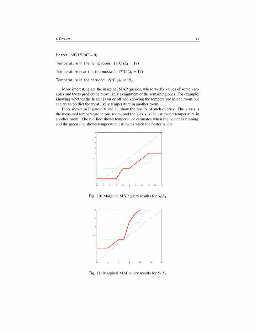
Heater: off (HVAC = 0)

Temperature in the living room: 18°C (S4 = 18)

Temperature near the thermostat’: 17°C (St = 17)

Temperature in the corridor: 19°C (S5 = 19)

More interesting are the marginal MAP queries, where we fix values of some vari-ables and try to predict the most likely assignment of the remaining ones. For example,knowing whether the heater is on or off and knowing the temperature in one room, wecan try to predict the most likely temperature in another room.

Plots shown in Figures 10 and 11 show the results of such queries. The x axis isthe measured temperature in one room, and the y axis is the estimated temperature inanother room. The red line shows temperature estimates when the heater is running,and the green line shows temperature estimates when the heater is idle.

14 15 16 17 18 19 20 21 22 23 2414

15

16

17

18

19

20

21

22

23

24

2

3

Fig. 10: Marginal MAP query results for St |S4

14 16 18 20 22 24 2614

16

18

20

22

24

26

2

4

Fig. 11: Marginal MAP query results for S5|S4

5 Conclusions 12

We can observe an interesting inversion of the HVAC effect on both plots. Untila certain point (around 18°C in Figure 10 and 20°C in Figure 11), the temperatureestimate with HVAC heating is lower than without it. Above this point, the effect isreversed, and estimates with the HVAC heating are higher than without it.

5 Conclusions

We have been able to design and build a small home sensor network and collect someuseful data. This dataset will be made public and available for future experiments.

We successfully modelled temperatures in a few rooms as Markov Random Fields,and estimated the MRF parameters from the collected data.

We have not been able to model the temperatures in all rooms or state of the doorsand windows as yet. The main reason is that during the initial planning of this project,we made an assumption that we would be able to do this using only unsupervised learn-ing techniques. Thus we have not collected information about the actual state of doorsor windows during the experiment. There were also some practical considerations forthis decision. Collecting door and window states would require us to design and buildadditional sensors, which would significantly expand the workload for this project.

6 Future Directions

With our sensor network running, we will keep collecting additional data. As seasonschange, we will get more diverse data. For example, we will finally get some datasamples in which the HVAC is engaged in cooling mode.

The most interesting future direction would be to try to predict the state of doors andwindows. This would require additional data collection with door and window sensors.Once such data is collected, we can use, for example, Conditional Random Fields(CRF) to model the conditional probability of doors and windows given temperaturesensor values.

It would be interesting to apply the methods we used in this project to differentdatasets, such as the one from CMU Sensor Andrew project [7].

Finally, we could try to use this model in some control algorithms. For example,we can control the setpoint of the thermostat to achieve a desired temperature in aparticular room of the house.

References

[1] DIGI INTERNATIONAL INC. XBee®/XBee-PRO®RF Modules. https://www.sparkfun.com/datasheets/Wireless/Zigbee/XBee-Datasheet.pdf.

[2] FALUDI, R. TMP36 instructions: Simple sensor network. http://www.

faludi.com/bwsn/tmp36-instructions-simple-sensor-network/.

[3] FALUDI, R. Building Wireless Sensor Networks: with ZigBee, XBee, Arduino,and Processing. O’Reilly Media, Incorporated, 2010.

6 Future Directions 13

[4] KOLLER, D., AND FRIEDMAN, N. Probabilistic graphical models: principlesand techniques. MIT press, 2009.

[5] KURLAND, V. Wireless temperature sensor. https://github.com/

vkurland/xbee_temp_sensor.

[6] RADIO THERMOSTAT COMPANY OF AMERICA. Wi-Fi USNAP mod-ule API version 1.3. http://www.radiothermostat.com/documents/

RTCOAWiFIAPIV1_3.pdf.

[7] ROWE, A., BERGES, M. E., BHATIA, G., GOLDMAN, E., RAJKUMAR, R.,GARRETT, J. H., MOURA, J. M., AND SOIBELMAN, L. Sensor andrew: Large-scale campus-wide sensing and actuation. IBM Journal of Research and Devel-opment 55, 1.2 (2011), 6–1.

[8] SCHMIDT, M. minFunc: Matlab uunconstrained optimization using line-searchmethods. http://www.di.ens.fr/~mschmidt/Software/minFunc.html,Apr. 2013.

[9] SCHMIDT, M. UGM: Matlab code for undirected graphical models. http://

www.di.ens.fr/~mschmidt/Software/UGM.html, Apr. 2013.

[10] SCHMIDT, M., AND MURPHY, K. Modeling discrete interventional data usingdirected cyclic graphical models. In Proceedings of the Twenty-Fifth Conferenceon Uncertainty in Artificial Intelligence (2009), AUAI Press, pp. 487–495.