home bias at home: local equity preference/media/dbf37883e3404efda278d34320… · the university of...

T h e U n i v e r s i t y o f C h i c a g o G r a d u a t e S c h o o l o f B u s i n e s s

Selected Paper 85

Home Bias at Home:

Local Equity Preference

in Domestic Portfolios

Joshua D. Coval

Harvard Business School

Tobias J. Moskowitz

The University of Chicago

Graduate School of Business

Joshua D. Coval

and Tobias J. Moskowitz

Joshua D. Coval is Associate Professor

at Harvard Business School, Boston,

Massachusetts 02163 ([email protected],

www.people.hbs.edu/jcoval).

Tobias J. Moskowitz is Associate

Professor of Finance at the University

of Chicago Graduate School of

Business, Chicago, Illinois 60637

([email protected],

gsb.uchicago.edu/fac/tobias.moskowitz).

We thank Michael Brennan, Bhagwan

Chowdhry, Gordon Delianedis, Mark

Grinblatt, Gur Huberman, Ed Leamer,

Tyler Shumway, two anonymous refer-

ees, editor René Stulz, and seminar

participants at MIT (Sloan) and

Michigan for helpful comments and

discussions. Moskowitz thanks the

Center for Research in Securities Prices

for financial support.

Publication of this Selected Paper

was supported by the Albert P. Weisman

Endowment.

Coval and Moskowitz, “Home Bias at Home: Local Equity

Preference in Domestic Portfolios” printed with permission

from Journal of Finance, published by Blackwell Publishing.

12-02/13M/CN/02-148

Design: Sorensen London, Inc.

Abstract

The strong bias in favor of domestic securities is a well-documented

characteristic of international investment portfolios, yet we show that the

preference for investing close to home also applies to portfolios of domestic

stocks. Specifically, U.S. investment managers exhibit a strong preference

for locally headquartered firms, particularly small, highly levered firms

that produce nontradable goods. These results suggest that asymmetric

information between local and nonlocal investors may drive the preference

for geographically proximate investments, and the relation between

investment proximity and firm size and leverage may shed light on several

well-documented asset pricing anomalies.

Joshua D. Coval and

Tobias J. Moskowitz

Home Bias at Home:

Local Equity Preference in Domestic Portfolios

S e l e c t e d P a p e r N u m b e r 8 52

The strong preference for domestic equities that investors in international markets

exhibit, despite the well-documented gains from international diversification,1

remains an important yet unresolved empirical puzzle in financial economics.

As French and Poterba (1991) document, U.S. equity traders allocate nearly 94 per-

cent of their funds to domestic securities, even though the U.S. equity market com-

prises less than 48 percent of the global equity market. This phenomenon, dubbed

the “home bias puzzle,” exists in other countries as well, where investors appear to

invest only in their home country, virtually ignoring foreign opportunities.

Although such behavior appears to be grossly inefficient from a diversification

standpoint, researchers have offered a variety of explanations for this phenome-

non. Initial explanations focused on barriers to international investment, such as

governmental restrictions on foreign and domestic capital flows, foreign taxes, and

high transactions costs.2 Although many of these obstacles to foreign investment

have substantially diminished, the propensity to invest in one’s home country

remains strong. Thus, two other categories of explanations have been put forth:

explanations associated with the existence of national boundaries (perhaps the dis-

tinguishing feature of international capital markets) and explanations associated

with a preference for geographic proximity. Under the first set of explanations,

when capital crosses political and monetary boundaries, it faces exchange-rate

fluctuation; variation in regulation, culture, and taxation; and sovereign risk, on

which many home bias explanations focus on as the primary factors discouraging

investment abroad. In addition, some other studies argue that informational dif-

ferences between foreign and domestic investors are the driving force behind

home bias, while others claim that investor concerns about hedging the output of

firms that produce goods not traded internationally are the primary cause.3

A key point largely overlooked in the debate, however, is that not all home bias

explanations rely on properties unique to the international economy. For instance,

while the existence of national boundaries may amplify information asymmetries

and the concern for hedging nontradable goods, these frictions arise even in the

absence of international borders, that is, when only geographic distance separates

an investor from potential investments. For example, investors may have easier

access to information about companies located near them, preferring to hold local

firms rather than distant ones over which they have a relative information advantage.

Local investors can talk to employees, managers, and suppliers of the firm, they

may obtain important information from the local media, and they may have close

personal ties with local executives, all of which may provide them with an informa-

tion advantage in local stocks. Likewise, investors may prefer proximate invest-

ments in order to hedge against price increases in local services or in goods not

easily traded outside of the local area. More generally, investors may have a prefer-

ence for geographically proximate investments potentially arising from a number

1 Grubel (1968); Solnik

(1974); Eldor, Pines,

and Schwartz (1988);

and DeSantis and

Gerard (1997), among

others, document

significant benefits

from diversifying

internationally.2 For examples of such

explanations, see

Black (1974) and Stulz

(1981a).3 Low (1993), Brennan

and Cao (1997), and

Coval (1996) offer

asymmetric informa-

tion–based explana-

tions of international

capital market segmen-

tation. Stockman and

Dellas (1989) and a

number of subsequent

papers suggest the

hedging of nontradable

goods consumption as a

motive for holding

domestic securities.4Huberman (1998)

finds that individuals

choose to invest in their

local Regional Bell

Operating companies

more often than any

other “baby Bell” even

though the companies

are listed on the same

exchange. The attrib-

utes such behavior to a

cognitive bias for the

familiar.5 Geography, which

continues to play a key

role in the domestic

economy despite sharp

declines in transporta-

tion and communica-

tion costs and vast

increases in informa-

tion technology, is the

subject of renewed aca-

demic debate. For

instance, Audretsch

and Feldman (1996)

C o v a l a n d M o s k o w i t z 3

of other sources. For instance, investors may simply feel more comfortable about

local companies or firms they hear a lot about, or they may have a psychological

desire to invest in the local community.4 In addition, local brokerage firms may

encourage local investment, particularly if close ties exist between brokers and

local corporate executives, for which some mutual benefit can be derived from

keeping local money in the community.

This paper investigates whether investors have a preference for geographically

proximate investments and assesses the importance of such a preference for port-

folio choice. Since geographic separation is certainly a factor in both domestic and

international settings, we analyze the effect of geographic proximity (distance) on

investment portfolio choice by restricting our attention to the domestic economy,

avoiding confounding factors due to political and monetary boundaries. If interna-

tional portfolio choice is influenced by frictions associated with distance, then

these frictions should play an identifiable domestic role as well.

More generally, this study supplements a recent resurgence in research docu-

menting the economic significance of geography and represents the first attempt to

uncover the effect of distance on domestic portfolio choice.5 This line of inquiry

not only highlights a potential new role for geography in the economy, but may also

shed light on various explanations for the international home bias puzzle.

Specifically, we measure U.S. money managers’ degree of preference for geo-

graphically proximate equities in their holdings of U.S.-headquartered companies.

Using a unique database of mutual fund managers and company locations, identi-

fied by latitude and longitude, we find that the average U.S. fund manager invests in

companies that are between 160 to 184 kilometers, or 9 to 11 percent, closer to her

than the average firm she could have held. Alternatively, one out of every ten com-

panies in a fund manager’s portfolio is chosen because it is located in the same city

as the manager. With a variety of measures used, the null hypothesis of no local

equity preference (or local bias) is consistently rejected, demonstrating that the

distance between investors and potential investments is a key determinant of U.S.

investment manager portfolio choice.

In addition, however, we wish to determine why U.S. investment managers, in

a setting of a single currency and relatively little geographic variation in regulation,

taxation, political risk, language, and culture, prefer to hold companies located

close to them.6 Some clues may exist in how the cross-section of firm and manager

characteristics relates to the degree of local investment preference.

We find that local equity preference is strongly related to three firm character-

istics: firm size, leverage, and output tradability. Specifically, locally held firms

tend to be small, highly-levered, and produce goods not traded internationally.

These results suggest an information-based explanation for local equity prefer-

ence, since small, highly levered firms, whose products are primarily consumed

test the importance of

geographic location for

innovative activity in

various industries, and

Audretsch and Stephan

(1996) examine the role

of university-based sci-

entists in local biotech-

nology firms. In addi-

tion, Jaffe, Trajtenberg,

and Henderson (1993)

show that knowledge

spillovers tend to be

geographically local-

ized, although this

localization fades over

time, and Lerner (1995)

finds distance to be an

important determinant

of the board member-

ship of venture capital-

ists, where venture cap-

ital organizations with

offices less than five

miles from a firm’s

headquarters are shown

to be twice as likely to

provide board members

to the firm as those

more than five hundred

miles away. For addi-

tional references on the

economic significance

of geography, see

Krugman (1991), Lucas

(1993), and Zucker,

Darby, and Armstrong

(1995).6 The clients of these

money managers could

be holding a geographi-

cally diverse set of

funds, and managers,

therefore, could be

investing locally in

order to minimize

information gathering

and travel costs.

However, Coval and

Moskowitz (1998b) find

that clients exhibit a

strong preference for

local managers.


locally, are exactly those firms where one would expect local investors to have easier

access to information and are firms in which such information would be most

valuable. Additionally, the importance of output tradability may lend empirical

support for the nontradable goods explanation of the international home bias

puzzle, although it is hard to believe that the role of internationally traded goods

output significantly affects proximity preferences in a domestic setting. Consistent

with these findings, Kang and Stulz (1997), in their examination of foreign owner-

ship of Japanese stocks, find that foreign investors underweight small, highly

levered firms and firms that do not have significant exports, which they claim may

be a response to the severe information asymmetries associated with such firms.

Furthermore, because size and leverage are associated with higher average

returns and aid in explaining the cross-section of expected stock returns,7 the

relation between the propensity to invest locally and these firm characteristics may

have important asset pricing implications. For example, Fama and French (1992)

argue that such characteristics may proxy for firm risk sensitivities, thus compen-

sating investors with higher average returns, while Daniel and Titman (1997)

suggest that it is the characteristics themselves that seem to be related to expected

returns, having little resemblance to risk. Although the interpretation of the rela-

tion between these characteristics and average returns can be debated, evidence

in this paper indicates that the influence of geographic proximity on portfolio

composition and these cross-sectional asset pricing anomalies may be linked in

an important way.

Finally, our analysis may offer insight for determining the importance of

distance in international portfolio choice relative to that of national boundaries,

assessing how much of the “home bias” phenomenon can truly be considered an

international puzzle. Extrapolating our findings to the international scale, we find

that distance may account for roughly one-third of the observed home country

bias in U.S. portfolios estimated by French and Poterba (1991). That is, as much as

one-third of the home bias puzzle may only be a feature of a geographic proximity

preference and the relative scale of the world economy, rather than a consequence

of national borders. These results should be interpreted only as qualitative evidence

of the importance of distance in the international setting, since the amount of

international home bias accounted for by a preference for geographic proximity

is sensitive to the form of extrapolation employed.

The remainder of this paper is organized as follows. Section I describes the

data and methodology employed in our study. Section II outlines and conducts a

test for local equity preference, and Section III examines the relation between

a variety of firm characteristics and the degree of proximity preference on portfolio

choice. Section IV extends the analysis to include a number of fund manager

characteristics, and Section V provides a summary and conclusion.

7 See Banz (1981),

Bhandari (1988),

and Fama and French

(1992). Fama and

French (1992) find

leverage and market-

to-book to be redun-

dant as firm distress

measures and find

market-to-book to have

greater explanatory

power for expected

returns. In our analysis,

firm leverage better

captures local equity

preference than

does the market-to-

book ratio.


I. Data and Methodology

Our primary data source is Nelson’s 1996 Directory of Investment Managers, which

contains the cross-section of 1995 holdings data on the largest U.S. money man-

agers along with their location (city and state). From Compact Disclosure, we

obtain the headquarters location of every U.S. company covered by that database.8

Using latitude and longitude data from the U.S. Census Bureau’s Gazetteer Place

and Zipcode Files, we match each fund manager and the headquarters of each U.S.

company with the latitude and longitude coordinates. To create our sample, we

identify the top ten holdings of each fund managed by a U.S. investment manager

and investing primarily in U.S. equities for 1995,9 which we define as those funds

for which at least five of the top ten holdings are U.S.-headquartered firms. Using

the coordinate data, we compute an arclength between each manager and every firm

in which the manager invests or could have invested.

To prevent outliers from dominating the analysis, we restrict our analysis

to the continental United States, excluding firms and funds located in Alaska,

Hawaii, or Puerto Rico. Although including fund managers and firms located in

these areas may potentially provide the strongest evidence for a geographic prox-

imity preference, our results are only slightly strengthened when we include these

funds and firms in the analysis. Since there are very few such funds and firms

in our sample, including them affects the results marginally. Hence, to be conser-

vative and concise, we exclude Alaskan, Hawaiian, and Puerto Rican funds and

firms. This also eliminates the possibility that our results are largely driven by

these remote locations exaggerating the effect of distance or are due to more

significant cultural differences between these three locations and the rest of the

continental United States.

Because we wish to focus on the behavior of managers that are in a position to

make portfolio choices, we exclude all index funds from the analysis. The dataset

also includes information on fund size, research sources, number of firms followed

by the manager, and whether the manager has any branch offices, as well as a

number of firm characteristics obtained from the 1995 COMPUSTAT tapes and the

1995 Compact Disclosure database.

Since a wide variety of restrictions prohibit mutual funds from investing in

certain companies, our universe of available assets consists only of companies

held by at least one mutual fund.10 Firms not covered by COMPUSTAT or Compact

Disclosure are also excluded. Furthermore, we ignore investments made by one

manager in another’s fund. While such investments may be locally biased as well,11

the funds may still ultimately end up invested in a geographically diversified

portfolio. Relatively few such investments occurred in our sample, and these are

excluded for simplicity. Thus, our final sample consists of 1,189 investment

8 We use the headquar-

ters location as opposed

to the state of incorpo-

ration for the simple

reason that companies

tend to incorporate in a

state with favorable

tax laws, bankruptcy

laws, etc., rather than

for any operational

reasons, and typically

do not have the majori-

ty of their operations

in their state of incor-

poration. In fact, very

few firms in our sample

were headquartered in

the state in which they

were incorporated.9 The Nelson’s dataset

records only the top

ten positions of each

investment manager.

The ten largest posi-

tions typically account

for about 30 percent of

a manager’s total asset

value.10Our results are largely

unchanged when we

expand the universe

to all 10,523 firms

for which we could

obtain data.11 Coval and Moskowitz

(1998b) find that

geographic proximity

plays a central role

in determining institu-

tional investors’

choice of investment

managers.


managers running 2,183 different U.S. equity funds with primary holdings in

2,736 different U.S. companies. These managers account for roughly $1.8 trillion of

investment in U.S. equities. Table 1 displays summary statistics for our database

of investment managers.

Figure 1 provides an overview of the geographic distribution of our sample of

fund managers and the companies they hold across the United States. The axes are

marked with the actual latitude and longitude degree values. Interestingly, the

graph’s distribution of firms and managers resembles a plot of U.S. population by

location, suggesting that companies and investment managers simply locate close

to the supply of human capital. Overall, investment managers appear to cluster

Table 1: Summary Statistics of U.S. Investment Managers

All data is from Nelson’s 1996 Directory of Investment Managers. Summary statistics on funds

managed by U.S.-based investment managers that invest primarily in U.S. equities, defined

as funds for which at least five of the top ten holdings are U.S.-headquartered firms, are

reported below. Fund managers located in Alaska, Hawaii, and Puerto Rico are excluded, as are

index funds. The average percentage of research and number of companies followed regularly

are obtained via a survey questionnaire that Nelson’s sends to each investment manager.

Managers are asked to allocate the percentage of research conducted among three categories:

(1) in-house, (2) on the street, and (3) consultant/other, as well as to report the number of

firms they follow on a “regular basis.”

Total number of managers 1,189

Managers with branch offices 426

Managers based in New York City 347

Number of funds under management 2,183

Total number of different companies held 2,736

Fund size (000’s) Mean $820,000

Median $149,000

Minimum $100

Maximum $ 28,702,000

Total $ 1,789,509,000

Average percentage of research In-house 66 %

Street 28 %

Consultant/other 6 %

Number of companies followed regularly Mean 748

Median 250

Minimum 8

Maximum 10,000


together more than companies do, suggesting that they are not simply locating close

to labor. For instance, the New York and Boston areas contain a disproportionate

share of managers relative to the rest of the country. However, there is generally a

fair degree of dispersion of managers throughout the country. In fact, managers

from all of the lower forty-eight states except Wyoming and the Dakotas are repre-

sented in our sample.

II. A Test for Local Equity Preference

Investors seem to exhibit preferences for certain securities based on a variety of

potential characteristics, including risk and return, liquidity, tax considerations,

and, possibly, several cognitive biases. In particular, Falkenstein (1996) and others

have shown that mutual fund managers also prefer certain types of stocks, for a

Figure 1: Geographic Distribution of U.S. Firms and Investment Managers

Plot of the location of the 1,189 investment fund managers in our sample and the headquarters

location of the 2,736 different companies they hold. The horizontal axis contains the actual

longitude, converted to degree values, of the fund manager and corporate headquarters

locations. The vertical axis contains the actual latitude degree values. Latitude and longitude

coordinates were obtained from the U.S. Census Bureau’s Gazetteer Place and Zipcode files.


variety of potential reasons. For instance, Falkenstein (1996) documents that

mutual fund managers prefer large, liquid stocks and stocks that belong to the S&P

500. However, to date, no one has examined whether investors, and in particular

fund managers, exhibit geographic preferences, particularly within a domestic

setting. In this section, we outline a test for geographically local preferences

among fund managers, attempting to control for other factors that might lead to a

spurious finding of such preferences. For example, if fund managers prefer stocks

belonging to the S&P 500 (regardless of their motivation) and these stocks happen

to cluster in the New York area, then it will appear as if fund managers prefer

New York–based stocks. If the managers also locate in the New York area, then it

will appear as if managers have a proximity preference, when in fact no such

preference may exist.

To assess manager preferences for local stocks while controlling for other

preferences managers might have, we conjecture an explicit null hypothesis that

claims deviations of manager portfolios from a prespecified benchmark should be

unrelated to distance. We begin, simply, with the Capital Asset Pricing Model

(CAPM) as our benchmark. However, our null hypothesis is not the CAPM, but

rather that deviations from the CAPM-implied portfolio weights are unrelated to

distance. We know that fund managers deviate from holding the market portfolio,

but these deviations should be unrelated to the manager’s distance from the com-

panies she is holding. In other words, each manager holds the market weight of

each security plus noise, where disturbances from market weights should be uncor-

related (under the null) with geographic proximity.

More formally, based on this intuition, our test statistic is developed as follows.

Suppose there are F different fund managers and n different securities in the

economy. Let mi,j represent the portfolio weight on stock j in the benchmark port-

folio for which fund manager i is compared. If the market portfolio is the relevant

benchmark for all funds, then mi,j is the same across all fund managers i and repre-

sents the market value weight of stock j in the economy. Next, let hi,j represent the

actual weight fund i places on stock j. We then compute the distance, di,j, between

fund manager i and the corporate headquarters of stock j, as follows:

di,j�arccos {cos (lati) cos (loni) cos (latj) cos (lonj)

�cos (lati) sin (loni) cos{ (latj) sin (lonj)�sin (lati) sin (latj)}2pr/360, (1)

where lat and lon are latitudes and longitudes (measured in degrees) of fund

manager and company headquarters location and r is the radius of the earth

(�6,378 km).


Finally, we compute the average distance of fund i from all securities j it could

have invested in, by weighting the distances between manager i and all n stocks in

the economy using the appropriate benchmark weights. More formally,

.(2)

With variables defined as above, our test for whether fund i exhibits a proximity

preference is stated in Proposition 1.

Proposition 1 Consider the test statistic which measures how

much closer fund manager i is to her portfolio than to her benchmark (as a fraction of the

distance she is from her benchmark). If deviations from the benchmark portfolio are

unrelated to the distance between manager i and the securities she chooses to hold, then

the null hypothesis H0 : LBi = 0 cannot be rejected.

Proof: Defining µ to be the unknown true mean of LBi, we can express the sam-

ple mean estimate as: 12

.(3)

Under the benchmark (in this case the market portfolio), the unconditional expec-

tation is that deviations from market portfolio weights are zero. Thus, µ will be

nonzero only if the second term is nonzero. In other words, the covariance between

portfolio weight deviations and distance (scaled) determines the value of LBi and

whether fund manager i exhibits a geographic proximity preference.

More generally, we compute the local bias test statistic, LBi, for all F fund

managers and aggregate the results. For ease of notation, let M denote an (F � n)

matrix in which elements of each row are weights of the n securities in some

benchmark portfolio, where the benchmark can differ for each of the F managers.

With the market portfolio as the benchmark for all managers, every row mi is the

same, where each row represents the market value weights of the n securities

in the market. In principle, however, the elements of M may differ across managers

(rows) to reflect other factors that may influence security choice, such as member-

ship in an index against which the particular manager is measured. Next, let H

denote an (F � n) matrix in which element hi,j reflects the actual weight of security

j in manager i’s portfolio, and define (F � n) matrix D such that element di,j is

the distance between manager i and security j. Next, let the matrix DM

denote the

(F � F) diagonal matrix of benchmark-weighted distances between a given manag-

er and her benchmark portfolio. That is, diagonal element �m8idi, where di

is the ith row of D. Finally, let w be an (F � 1) manager weighting vector whose

elements are nonnegative and sum to one. That is, w assigns weights to fund

managers to determine the importance (contribution) each manager has on the

12 Here, distance can

be viewed as a random

variable, since fund

managers choose which

securities to hold and

the weights assigned

to them in the portfolio,

both of which determine

the average distance

a fund manager is from

her holdings.


test statistic. Two weighting schemes are employed: (1) equally weighting each

manager [i.e., w equals an (F �1) vector with all elements equal to 1/F], and

(2) value weighting each manager by the fraction of aggregate total asset value each

fund comprises.

The test statistic, LB, is defined as:

LB ¨w8 diag(( M�H)(D8(DM)�1)) (4)

with sample moment estimates:

µ � w8 diag(E(M�H)E (D8(DM)�1 � Cov (M�H, D8(D

M)�1))(5)

s2� w8(diag(( M�H)(D8(DM)�

((M�H)(D8(DM)�1)))2 (6)

where Cov(X,Y ) represents the element by element covariance between the entries

in matrices X and Y.

A positive LB measure indicates a preference for geographically proximate

equities, and a negative measure signifies a preference for distant firms. As the

number of fund managers (F) becomes large, LB approximately follows a normal

distribution, so test statistics on LB can be computed via sample means and variances

and a simple mean test on LB can be applied. In addition, we have defined distances

as percentages or scaled values of a manager’s average distance from all stocks

(i.e., D8(DM)�1) in order to normalize distances across fund managers and

reduce heteroscedasticity in manager-holding distances. For instance, a fund man-

ager in Seattle is much farther away from the average stock than is a manager in

Chicago and thus may be given more importance and will have higher distance vari-

ances than the Chicago-based manager if distances are not scaled appropriately.

This is the basis for our tests of local equity preference. While our benchmark

portfolio has thus far been the market, in subsequent tests we employ other bench-

mark weights as well. For instance, the relevant benchmark for aggressive growth

fund managers would be the aggregate aggressive growth index, defined as the

universe of stocks held by aggressive growth fund managers. Therefore, for this

subset of managers, the LB statistic measures deviations from the relevant aggres-

sive growth index that are correlated with distance. Similarly, a small stock index is

employed as the relevant benchmark for small company managers, and so forth.

Thus, the elements of M differ across managers (rows) to reflect their relevant

benchmarks and other influences on security choice. Redefining the benchmark in

this manner for subsets of managers alleviates concerns about spurious rejection of

the null hypothesis, since managers from each subset are compared relative to the

average manager from that subset. Thus, the exogenous location of aggressive

growth fund managers, for example, and of growth stocks cannot drive rejection of


the null, since the benchmark portfolio weights already account for the fact that

such managers happen to be located near growth stocks. In other words, only

deviations in relative portfolio weights (relative to other aggressive growth funds)

and their correlation with (scaled) distance can lead to rejection.13

A. Empirical Results

Table 2 presents the results for our tests of local equity preference. The tests differ

in terms of the benchmark portfolio weights, M, and the manager-weighting vec-

tor, w. When firms are equally weighted, the elements of M are all 1/n (i.e., the

benchmark portfolio is the equal-weighted index of all stocks being held by at least

one fund), and when firms are value-weighted, each column j is firm j’s fraction

of total market capitalization. When funds are equally weighted, the elements

of w are all 1/F, and when funds are value-weighted, element wi is manager i’s

fraction of the total $1.8 trillion under management by our sample of fund man-

agers. In addition to reporting the local bias measure, LB, Table 2 also reports the

components that comprise the LB statistic. Column 2, for instance, reports the

average distance of fund managers from the securities they hold in their portfolios

(i.e., w8diag(HD8)). Column 3 reports the average distance of fund managers

from their benchmark portfolio (in this case, either the equal or value-weighted

index), which is computed as w8diag(MD8). Column 4 reports the difference

between columns 2 and 3, which represents how much closer (in km) managers are

actually investing their money relative to their benchmark portfolio. Finally, col-

umn 5 reports the LB measure (as a percentage), which is simply column 4 divided

by column 3 (multiplied by 100), or equivalently, w8 diag

((M�H)(D8(DM)�1)).

As shown in Table 2, fund managers are on average between 1,654 and

1,663 kilometers away from the securities they hold, yet are between 1,814 and

1,847 kilometers away from their benchmark portfolio. Thus, the average manager

invests in securities that are 160 to 184 kilometers closer to her than is her bench-

mark portfolio. In percentage terms, managers are investing in securities that are

9.32 percent to 11.20 percent closer to them than the average security in their

benchmark portfolio is. From columns 5 and 6, we see that the null hypothesis

of no local bias is soundly rejected in all test specifications and appears to be

economically significant.

Finally, since many firms and funds are clustered around New York City

(N.Y.C.), our finding of a local bias may be driven by the exogenous concentration

of companies and managers in this area. Therefore, we remove the 347 New York

City–based fund managers from our sample, defined as managers located within

100 kilometers of downtown New York, and recompute our test statistics. As Table 2

shows, the existence of a strong proximity preference is robust to the exclusion of

13 Of course, if location

is endogenous, and

under the null, distance

is unimportant, then

there is no ex ante

reason that aggressive

growth fund managers

should be located

near growth stocks.

Therefore, in this case,

the benchmark model

of the CAPM (market

portfolio) seems appro-

priate for all subsets

of fund managers.

We ran both sets of

tests, however, for

robustness, and found

very little difference in

the results. Therefore,

compared to the aver-

age manager in the

economy and to the

average manager in a

particular subset, the

preference for local

equities is exhibited

strongly.


N.Y.C. fund managers.

A.1 Regional, Sector, and Small-Cap Funds

In addition, our results may be driven by a particular class of fund managers. For

instance, there are a number of funds that invest only in stocks from a particular

region. If location is unimportant for investing, then these funds can presumably

be run from any location and thus do not necessarily need to be located in the

region in which they are investing. However, it is interesting to see if a predomi-

nant local bias remains once we exclude regional funds. We also control for two

other types of funds: sector and small-cap funds. Sector funds are excluded because

stocks in the same industry or sector tend to cluster geographically and thus may

provide another interesting subset of funds to examine. In addition, because of the

Table 2: Test for Local Equity Preference among All Nonindex Funds

Tests for local bias among the 2,183 nonindex funds in our sample (1,836, excluding funds

based in New York City) are reported below. All combinations of equal and value-weighted funds

and firms are reported, where value weights for firms (M) are the firm’s fraction of total market

capitalization, and value weights for funds (w) are the fund’s fraction of total aggregate asset

value under management. Also reported are the components that comprise the local bias

statistic, LB. Column 2, for instance, reports the average distance of fund managers from the

securities they hold in their portfolios (i.e., w8diag (HD8)), where w is the weighting vector

applied to the F funds, H is the (F � n) matrix of actual portfolio weights each of the F fund

managers applies to the n stocks in the economy, and D is the (F � n) matrix of distances

between fund managers and the headquarters of each stock in the economy. Column 3 reports

the average distance of fund managers from their benchmark portfolio (in this case either the

equal- or value-weighted index), which is computed as w8diag (MD8), where M is the (F � n)

matrix of benchmark portfolio weights to which fund managers are compared. Column 4 reports

the difference between columns 2 and 3, which represents how much closer (in km) managers

are actually investing their money relative to their benchmark portfolio. Finally, column 5 reports

the LB measure (as a percentage), which is simply column 4 divided by column 3 (multiplied

by 100), or equivalently w8diag ((M�H)(D8 (DM)�1)). The t-statistics for LB are reported in the

last column. In addition, tests are run excluding funds located in New York City.

Weights Average Distance from

Funds (w)–Firms (M) Holdings Benchmark Difference % Bias (LB) t-stat

Equal-Equal 1,654.18 1,814.59 160.41 9.32 14.28

Equal-Value 1,654.18 1,830.32 176.15 10.31 15.93

Value-Equal 1,663.09 1,833.30 170.21 10.27 15.21

Value-Value 1,663.09 1,847.44 184.35 11.20 16.82

Equal-Equal (ex-N.Y.C.) 1,685.73 1,841.03 155.30 8.95 13.36

Value-Value (ex-N.Y.C.) 1,734.71 1,892.32 157.61 9.61 13.95


large number of funds focusing on small capitalization stocks, it is interesting to

determine if these funds primarily drive the local bias phenomenon. Before

excluding these funds from the analysis, however, we run our tests on each of these

subsets of funds individually. Results are presented for tests in which firms and

funds are both equally and value-weighted. As stated earlier, the benchmark port-

folios are adjusted in each test to reflect the equal and value-weighted portfolio

appropriate for the class of manager being tested. For instance, for small-cap

funds, the appropriate benchmark portfolio is the aggregate small-cap fund hold-

ings of all stocks held by at least one small-cap fund manager. In other words,

deviations in portfolio weights of a particular manager are measured relative to the

aggregate holdings of all small-cap managers. Similar benchmarks are employed

for the regional and sector funds, as well as all other funds not classified under any

of these categories.

As Table 3 demonstrates, the fourteen regional funds exhibit a considerable

local bias. The average regional fund holds a portfolio biased between 42 and

53 percent in favor of local securities. This provides additional evidence that

investors prefer to be near the pool of investments from which they select, for if

investors had no preference for investing in nearby securities, then a fund such as

Capital Consultants’ WestCap Equity fund (a fund focusing on companies head-

Table 3: Test for Local Equity Preference Across Fund Types

Tests for local bias among four subsets of funds—regional, sector, small-cap, and all others—are

reported below. For each subset of funds, the number of managers, average weighted distance

from securities held, average distance from the relevant benchmark portfolio, and the difference

between these two measures (both in actual km and in percentage terms) are reported. The

benchmark portfolio consists of only those stocks being held by at least one fund in the subclass

of funds being analyzed. Both equal- and value-weighting schemes are employed to funds and

firms, and t-statistics on the local bias measure are provided in the last column.

Weights Average Distance from

Fund Type Firms-Funds Holdings Benchmark Difference % Bias t-stat

Regional: Equal-Equal 705.73 1,593.25 887.52 53.06 6.55

(n=14) Value-Value 983.60 1,701.82 718.21 41.79 4.89

Sector: Equal-Equal 1,737.04 1,801.11 64.07 3.18 0.78

(n=85) Value-Value 1,672.43 1,892.85 220.42 11.62 2.79

Small-Cap: Equal-Equal 1,755.36 1,879.40 124.03 5.69 3.88

(n=435) Value-Value 1,814.25 1,758.25 �55.99 �5.52 �3.69

All Others: Equal-Equal 1,625.83 1,793.85 168.02 10.24 14.03

(n=1676) Value-Value 1,645.27 1,853.81 208.54 12.74 16.80


quartered in the ten western states) could be just as easily run out of New York City

as out of Portland, Oregon, its current headquarters.

The local bias results for sector and small-cap funds are somewhat more

ambiguous and depend heavily on whether equal or value-weighted specifications

are employed. The 85 sector funds exhibit between 3.2 percent and 11.6 percent

local bias, whereas the 435 small-cap funds exhibit between 5.7 percent and

-5.5 percent bias. Since both types of funds are more constrained in terms of the

set of securities in which they may invest, these results are not entirely unexpected.

For example, an automotive sector fund located on the East Coast simply will not be

in a position to bias locally, because there are few local automotive firms. Likewise,

the scope for investment by small-cap funds is limited to regions experiencing

high economic growth, independent of their proximity to the manager. On the

other hand, if distance is important, managers of such funds should locate near the

pool of securities in which they expect to invest, much like the regional funds

appear to do. One reason this may not be taking place is that unlike regional funds,

small-cap and sector funds are usually part of a large investment firm’s family of

funds. Therefore, a firm such as Fidelity, with more than thirty different sector

funds, will be highly limited in its ability to locate near the firms in each of these

sectors, so the degree of local bias among sector funds may be somewhat weak. The

same may be true for small-cap funds. This is consistent with the empirical evi-

dence, as regional funds are typically run by a single manager from a small invest-

ment firm, while both sector and small-cap funds are generally part of the largest

investment firms’ array of funds. However, the negative local bias measure for the

value-weighted specification of small-cap funds is puzzling, although this apparent

preference for geographically remote firms is quite small, only 56 km farther away

than the average small capitalization stock. Most importantly, however, is the fact

that when regional, sector, and small-cap funds are removed from the sample, the

degree of local bias increases to between 10.2 percent and 12.7 percent, verifying

that the preference for proximate investments is indeed a broad phenomenon not

driven by or restricted to a particular class of fund managers.

B. Comparison to International Home Bias

Thus far, we have established that a significant geographic preference for proxi-

mate firms exists among professional money managers within a domestic setting.

How important is this proximity preference in the international setting? To get a

qualitative idea of the significance of our results in the context of the international

home bias evidence, we project our findings onto the international scale by extrap-

olating our results using global distances. In this way, we can obtain a rough meas-

ure of how much of the home bias in international portfolios can be attributed

solely to a preference for geographic proximity.


Our most conservative domestic results, when firms and managers are

equally weighted, reveal a 9.32 percent local bias, where the average security is

1,815 kilometers away from the average fund manager. Determining how much of

the international home bias can be attributed to a preference for local securities,

given the vast distances separating investors from potential investments in the

global setting, may be difficult. One possibility is simply to allow for a linear extrap-

olation of our results—to shift 9.32 percent of the market capitalization weight of a

country in the global market portfolio to the domestic economy for every 1,815 kilo-

meters that separate the country from the investor. A potential problem with this

approach is that it may induce short positions in very distant countries. Another

possibility is to reduce overseas holdings proportionately by shifting 9.32 percent

of the country’s remaining portfolio weight to the domestic economy for every

1,815 kilometers that separate the country and the investor. With s as the home

country’s share of the world market and d as its distance from the investor, each

country’s distance-adjusted portfolio share is computed as sd�s*(1�0.0932) . Table 4 compares the weights of Japan, the U.K., France,

Germany, Canada, and

the U.S. in the world market portfolio (1) to weights of portfolios constructed using

proportional extrapolation of our calculated domestic distance effect to interna-

tional scales, and (2) to French and Poterba’s (1991) estimates of the U.S. portfolio

Table 4: The Distance Effect on U.S. Equity Portfolio Weights

Market capitalization weights of the U.S., Japan, U.K., France, Germany, and Canada in the

world market portfolio are compared (1) to actual weights assigned by U.S. investors to these

countries based on the results from French and Poterba (1991) using 1989 capital flows

data, and (2) to distance-adjusted weights calculated by shifting 9.32 percent of a country’s

remaining market capitalization weight to the U.S. for every 1,815 km that separate the country

from the U.S. (New York City). With s as each country’s share of the world market and d as

its distance from the U.S., each country’s distance-adjusted portfolio share is computed as

s d�s * (1�0.0932) .

Portfolio Weights Market Actual Distance- Distance from

Weight Weight Adjusted N.Y.C. (km)

U.S. (New York) 0.478 0.938 0.655 0

Japan (Tokyo) 0.265 0.031 0.147 10918

U.K. (London) 0.138 0.011 0.102 5,602

France (Paris) 0.043 0.005 0.031 5,871

Germany (Frankfurt) 0.038 0.005 0.028 6,042

Canada (Toronto) 0.038 0.010 0.037 551


share allocated among these countries at the end of 1989.

As illustrated in Table 4, distance may indeed account for a substantial portion

of the home bias phenomenon. The distance-adjusted portfolio weights appear to

move portfolio shares about one-third of the way between the market and actual

weights. In other words, perhaps up to one-third of the home-bias puzzle is not an

international puzzle at all, but merely a feature of the scale of the world economy

and a preference for proximate investments. The distance or proximity effect

explains some of the relative U.S. holdings, as well. For example, Canadian equities

represent a smaller share of the world portfolio than those of either Germany or

France, yet they account for twice as much of the average U.S. portfolio. When dis-

tance is taken into account, the picture improves substantially, as the Canadian dis-

tance-adjusted weight is larger than that of Germany or France, consistent with the

actual weights U.S. investors assigned to these countries.

The above computations raise several issues worth considering. First, our

measures of local bias focus solely on investment manager holdings. However,

since individual investors hold almost half of all U.S. equity, a measure of their

degree of local preference is required for a complete assessment of the distance

effect in both domestic and international settings. However, our calculations for

fund manager local preference may be closer to a lower bound on individual

investor local preferences, since individuals likely exhibit stronger geographic

preferences than do professional money managers. For instance, if local equity

preference is the result of a local information advantage, then individual investors

trading distant securities are expected to be at an even greater disadvantage than

are institutional investors, who have extensive resources, research facilities, and

contacts that make information easier to acquire. The international evidence

appears to support this view, as institutions account for a relatively large share of

U.S. investment holdings abroad. Thus, our results appear conservative and will

likely be strengthened if individual investor preferences are included.

Second, we should consider the possibility that while managers bias locally,

clients of the fund may diversify geographically among managers. Thus, the correct

metric to apply to the international setting is actually a product of clients’ local

manager preference and managers’ local stock preference. This issue is addressed

by Coval and Moskowitz (1998b), who investigate client selections of investment

managers and find that clients tend to invest with managers that are roughly 30

percent closer than is the average manager. When extrapolated to international

distances, this suggests that clients are highly averse to investing with managers

based overseas. As a result, we remain confident that the above calculations, while

somewhat crude, are a fairly realistic picture of the effect of distance on interna-

tional portfolio holdings.

Finally, distance itself, particularly in the international context, might be more


usefully thought of in terms of “economic distance.” For example, compared with

Paris in economic terms, London may be considerably closer to New York than the

269-kilometer (4.5 percent) difference in physical distance suggests. Integrating

information contained in varying languages, cultures, airline routes, and phone

rates, for example, may provide a richer characterization of the financial frictions

associated with geographic distance. Qualitatively, however, geographic distance

alone appears relevant for both domestic and international portfolio choice.

III. Local Bias and Firm Characteristics

More generally, whether or not a geographic proximity preference is responsible

for or contributes to the international home bias phenomenon, we wish to under-

stand why a proximity preference exists, particularly among professional money

managers. In this section, we examine whether the preference for local equities

varies across different kinds of firms. Identifying traits common to locally favored

firms will improve our understanding of why investment managers bias their port-

folios locally. We begin by examining the relation between the propensity to invest

locally and a variety of firm characteristics, including accounting numbers, market

values, employment figures, and sector data.

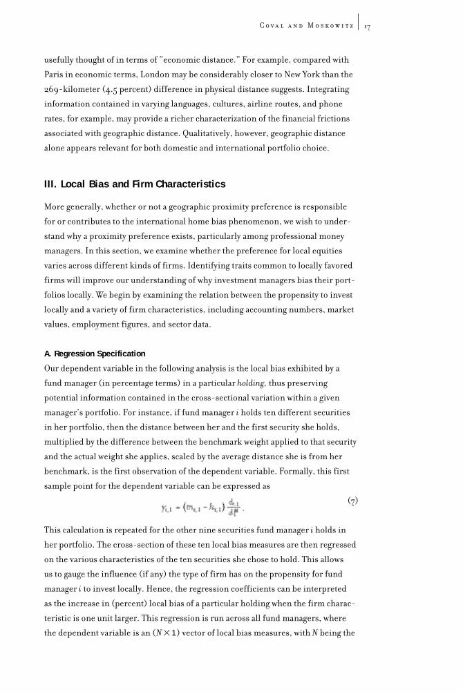
A. Regression Specification

Our dependent variable in the following analysis is the local bias exhibited by a

fund manager (in percentage terms) in a particular holding, thus preserving

potential information contained in the cross-sectional variation within a given

manager’s portfolio. For instance, if fund manager i holds ten different securities

in her portfolio, then the distance between her and the first security she holds,

multiplied by the difference between the benchmark weight applied to that security

and the actual weight she applies, scaled by the average distance she is from her

benchmark, is the first observation of the dependent variable. Formally, this first

sample point for the dependent variable can be expressed as

.(7)

This calculation is repeated for the other nine securities fund manager i holds in

her portfolio. The cross-section of these ten local bias measures are then regressed

on the various characteristics of the ten securities she chose to hold. This allows

us to gauge the influence (if any) the type of firm has on the propensity for fund

manager i to invest locally. Hence, the regression coefficients can be interpreted

as the increase in (percent) local bias of a particular holding when the firm charac-

teristic is one unit larger. This regression is run across all fund managers, where

the dependent variable is an (N�1) vector of local bias measures, with N being the


total number of fund manager holdings (N�18,187).

The cost of such an approach is that now the error terms will no longer

be independent across a particular manager’s portfolio. To accommodate this

correlation, we run a Feasible Generalized Least Squares regression (FGLS) to

allow for nonzero off-diagonal elements of the error variance-covariance matrix.

Specifically, letting Y be the (N�1) vector of dependent variables and defining

X as the (N � k) matrix of independent variables, where k is the number of

firm characteristics we explore to describe the degree of local bias, our regression

model is expressed as

y�X b�e, (8)

E(ee8)�s2V, (9)

where b is the (k�1) vector of coefficients on the firm characteristics, s2 is a

scalar, and V is an (N�N) matrix with element v i,j�1 if i�j, v i,j�r if holdings

i and j belong to the same fund manager, and v i,j�0 otherwise. Using the iterative

two-step procedure of Oberhofer and Kmenta (1974), we estimate r jointly

with b and s2.

B. Multivariate Regressions

For brevity, the results reported for the remainder of the paper correspond to a

benchmark portfolio of the equally weighted index. However, our results are largely

unchanged when we use a value-weighted index as the benchmark for the depend-

ent variable. The first three regressions incorporate the same firm characteristics

as those in Kang and Stulz (1997): firm size (market capitalization), leverage, cur-

rent ratio, return on assets, and market-to-book ratio. A fourth regression adds

firm employees and a tradable/nontradable dummy variable explained below.

The first regression (regression A) includes only the log of firm size. As men-

tioned earlier, Kang and Stulz (1997) find that foreign investors overweight large

firms when investing in Japanese equities. They argue that this behavior may be

related to the lower information asymmetries associated with large firms. Including

firm size in our regression allows us to address whether this effect is present within

a domestic setting and thus whether it is related to distance.

In the second regression (regression B), we add a pair of accounting figures,

leverage and the current ratio, to the first regression. Leverage, defined as the ratio

of total liabilities to total assets, is often used as a measure of firm distress, and the

current ratio, which measures the ratio of current assets to current liabilities, cap-

tures the short-run financial health of a firm. Thus, the current ratio complements

the leverage variable, allowing us to identify the horizon at which financial distress

may be most important.


In the third regression (regression C), we add return on assets and the market-

to-book ratio to the other three firm characteristics. A firm’s return on assets

(ROA), defined as the ratio of income before extraordinary items divided by total

assets plus accumulated depreciation, is a useful measure of accounting perform-

ance. Firm market-to-book ratios provide a measure of a firm’s potential growth

and may indicate whether managers prefer local firms that have experienced price

run-ups and whose market values may reflect substantial growth opportunities. It

is also possible that the market-to- book ratio represents a systematic firm distress

factor as Chan and Chen (1988) and Fama and French (1992, 1993, 1996) argue. If

market-to-book ratios signal the exposure of firms to an economy-wide distress

factor, then we can see whether investors respond differently to a firm’s relative

distress sensitivity, depending on their proximity to the firm.

Finally, in the fourth regression (regression D), we look at the number of

employees of the firm and the tradability of firm output in relation to local bias, by

adding these variables to our model. The number of employees helps determine

whether managers obtain information from the labor side of production. In partic-

ular, if managers obtain private information through the employees of local firms,

manager holdings may be concentrated in firms with more employees. The number

of employees also provides a non-market-value measure of a firm’s size. To assess

the impact of output tradability, we include a dummy variable identifying firms that

had positive total foreign sales recorded in COMPUSTAT’s 1994 Geographic

Segment File. Of our sample of firms, 37 percent were assigned a tradable-goods

indicator (i.e., had positive foreign sales). Examining output tradability is support-

ed by a number of authors who have argued that investors may be concerned with

the correlation between the return on their investments and the degree of avail-

ability of the goods that they consume.14 In particular, Stockman and Dellas (1989)

argue that investor concern over the correlation between investment returns and

their consumption of nontradable goods compels them to hold equity in firms that

produce these goods. If these motives are important for investment managers, we

should expect them to overweight local firms that produce nontradable goods.

However, our measure of tradability, whether a firm had positive foreign sales, is

probably a very crude measure of the tradability of a firm’s output in a domestic set-

ting. While some of the firms with no foreign sales do in fact produce goods not

easily transferable across distances (i.e., construction, highways, services, etc.),

others may produce highly tradable products that simply do not traverse interna-

tional boundaries for any number of reasons. Thus, the tradable dummy variable

may be better interpreted in an informational role, as Kang and Stulz (1997) sug-

gest, where the relation between the export propensity of firms and foreign owner-

ship may be due to information asymmetries rather than concerns for hedging

nontradable goods.15

14 This proposed rela-

tion is not necessarily

straightforward,

however. For examples

of such models, see

Stulz (1981b), Adler

and Dumas (1983),

Stockman and Dellas

(1989), Backus and

Smith (1993), Tesar

(1993), Uppal (1993),

Ghosh and Pesenti

(1994), and Serrat

(1997).15 We thank the referee

for pointing this out.


16 Fama and French

(1992) find that lever-

age and market-to-

book are redundant

firm distress factors,

but that market-to-

book has stronger

explanatory power

for capturing cross-

sectional variation in

expected returns. In

terms of explaining the

propensity to invest

locally, we find leverage

to have greater explana-

tory power.


Table 5: Multivariate Regression (Firm Characteristics)

The dependent variable in the following regressions is the local bias exhibited by a fund manag-

er in a particular holding. The local bias of each holding is calculated as a percentage by multi-

plying the distance between the manager and each of her holdings by the difference between

her benchmark weight applied to each stock and the actual weight she assigned to each stock,

divided by the weighted average distance the fund manager is from her benchmark. More

formally, where mi,j is the portfolio weight of stock j in fund manager

i’s benchmark portfolio, hi,j is the actual weight fund manager i assigns to stock j, di,j is the

distance between manager i and stock j, and is the weighted average distance between

manager i and her benchmark (i.e., ). The regression is run across all fund

managers and all of their holdings (18,187 observations) on various firm characteristics. The

benchmark portfolio employed is the equal-weighted index of all stocks held by at least one

fund. Regressions are run using a Feasible Generalized Least Squares (FGLS) procedure

described in section A, where the correlation estimate, r(%), from that procedure is reported

at the bottom of the table. Coefficient estimates on the firm characteristics are reported, along

with their t-statistics in parentheses.

Regression A B C D

Constant 22 & 86** 16.74* 17.48** 17.12**

(3.50) (2.60) (2.71) (2.33)

In (MV) �0.60* �1.46** �1.53** �1.39**

(�2.07) (�5.04) (�5.20) (�4.10)

Leverage 42.65** 43.16** 40.60**

(18.24) (18.33) (16.93)

Current Ratio 0.24 0.26 0.29

(0.50) (0.55) (0.62)

Return on Assets –1.25** �1.21**

(�2.91) (�2.84)

Market-to-Book Ratio 0.15 0.23

(1.23) (1.85)

Employees 0.02**

(4.33)

Tradable Dummy �7.91**

(�6.76)

r 9.50 8.81 8.79 8.85

*Significant at 5 percent level. **Significant at 1 percent level.

diM

� � mi,j di,jj

di

�M

d iM��

di,1 �yi,1 = �mi,1 − hi,1�

A

i,j�


C. Empirical Results

Table 5 reports the results of our regressions of local bias on these various firm

characteristics. As the table demonstrates, size, leverage, and the tradable-goods

dummy are highly economically and statistically significant in all regressions.

Examining the results from regression A, we see that managers’ investments in

large firms tend to be further away than those in small firms, as the size coefficient

is significant at the 5 percent level. Controlling for other firm characteristics,

primarily leverage, the size coefficient is significant at the 1 percent level. Moreover,

a one-standard-deviation increase in log size increases the propensity to invest

locally by 2.8 percent to 3.1 percent, indicating an economically significant relation

between size and degree of local bias as well. This result is consistent with Kang and

Stulz (1997), who find that foreigners prefer larger firms when investing in the

Japanese market and suggests that the preference for large Japanese equities is at

least partly due to a proximity preference rather than a national border effect.

Turning next to our distress variables, leverage is highly significant, with

t-statistics over 18, and a one-standard-deviation increase in leverage is associated

with holdings biased approximately 10 percent closer to the manager. When we

control for other characteristics, the significance of the leverage coefficient

remains unchanged. This result is also consistent with the findings of Kang and

Stulz (1997), although they find that the foreign investor preference for low-

leverage firms disappears when controlling for size. The current ratio, however, is

insignificant, suggesting that important firm distress information is better cap-

tured by the long-run leverage measure than by the short-run current ratio.

In regression C, the return on assets is significant at the 1 percent level, indi-

cating that investors favor local firms with relatively poor accounting performance.

However, this preference is not manifested in an economically important way. To

illustrate, consider a holding that has a return on assets of 26.9 percent (20 percent

above the mean). Although fewer than 1 percent of all holdings enjoy such a high

ROA, this translates into a decrease in local preference of only 0.33 percent. Thus,

a firm’s return on assets appears, at best, marginally important in accounting for

local bias. The lack of significance of the market-to-book ratio for explaining local

bias is likely due to the strong explanatory power of the leverage variable in captur-

ing firm distress. Thus, leverage appears to be the only relevant firm distress vari-

able accounting for local bias.16

Finally, in regression D, with the addition of the number of firm employees

as well as the tradable-goods dummy, both variables are significant at the 1 percent

level, yet only the tradable-goods dummy appears economically important. A one-

standard-deviation increase in number of employees increases local bias only by

0.2 percent. On the other hand, holdings of firms whose output is nontradable,

as measured by an absence of foreign sales, exhibit a 7.9 percent greater bias than

17 Whether this is or is

not the case is beyond

the scope of this

paper. However, for an

analysis of the relative

importance of borders

and distance in inhibit-

ing the tradability

of goods between the

United States and

Canada, see Engel and

Rogers (1996).18 Merton (1987), 489.


firms producing tradable goods. This finding is consistent with the international

evidence of Kang and Stulz (1997), who document a preference by foreign investors

for firms with substantial exports, which may indicate the lower degree of infor-

mation asymmetry associated with these firms. Likewise, firms with primarily

local sales have higher information costs and may be difficult to evaluate at a

distance. The preference of local money managers for these firms is consistent

with this information story, since local managers, who presumably have a local

informational advantage, can better exploit that advantage in these firms. In addi-

tion, the strong relation between the tradable-goods dummy and local bias may

lend support to nontradable goods hedging explanations for the international home

bias puzzle, if the tradability of goods is just as likely associated with distance as

with political boundaries.17

D. Implications for Informed Trading

Overall, the regression results support an information-based explanation for local

equity preference. In addition to the interpretation of our results for the tradable-

goods variable, the relation between the degree of proximate investment and

size and leverage is perhaps the best evidence of an asymmetric information inter-

pretation for the effect of distance on portfolio choice. For instance, Merton (1987)

argues that there are several important costs associated with the conveyance of

useful information from the firm to the investor. Not only must the firm take

steps toward signaling accurate information, but the investor also needs to be

equipped to receive these signals. Since a particular manager cannot follow all

publicly traded securities, Merton (1987) argues that investors select specific firms

for which to incur “receiver setup costs.”18 If such costs are similar in absolute

terms across firm size, then, relative to the costs of trading such information

(i.e., liquidity costs) these costs are larger in smaller firms. Of course, ceteris

paribus, investors are compensated for these costs. The question, though, is which

investors will do so most willingly. Clearly, investors with lower fixed setup costs

will choose to incur the costs. In the present case, it seems that proximity may

be lowering this fixed cost, with small firms offering the proportionately largest

decline. As a result, local investors appear to have the largest comparative

advantage trading in small firms.

Our finding that leverage significantly accounts for local bias cannot be fully

explained by receiver setup costs, however, as it is difficult to see why highly lev-

ered firms should have relatively lower setup costs for local investors. The signifi-

cance of the leverage variable is most likely accounted for by its association with

future earnings variance, i.e., highly levered firms have greater future returns

uncertainty. Coval (1996) shows that this variance is associated with larger holdings

by informed investors do. Because uninformed investors face more severe adverse


selection when investing in such securities, they hold relatively smaller propor-

tions than informed investors. If local investors obtain superior forecasts of future

returns, their shares should be largest in firms for which these forecasts are most

valuable. Of course, the same argument also applies to small firms, whose cash

flows appear more volatile as well.

Perhaps the more intriguing result is that the size and leverage firm characteris-

tics have been identified as significant explanatory variables for the cross-section

of expected returns. Numerous studies have documented the apparent abnormal

returns associated with small, highly levered firms. Fama and French (1992, 1993,

1996) suggest that such firm characteristics proxy for earnings risk factors, compen-

sating investors with higher average returns. This point is consistent with the find-

ings of Shumway (1996), who shows that firm size and leverage are important in

constructing bankruptcy hazard rates. The evidence presented here suggests that

because local investors have more accurate estimates of future earnings prospects,

they may expose themselves more willingly to earnings risk factors. In other words,

investors are willing to place larger and riskier bets on firms they know more about.

Thus, risky firms (i.e., small, highly levered firms) are more likely to be held by

local investors. Another possibility is that if size and leverage are proxies for system-

atic risk, then perhaps local investors understand local firms’ exposure to these

factors better than nonlocal investors do. Thus, an apparent relation between size

and leverage and the propensity to invest locally will exist. Alternatively, size and

Table 6: Multivariate Regression (Firm and Manager Characteristics)The dependent variable in the following regressions is the local bias exhibited by a fund

manager in a particular holding. We calculate the local bias of each holding as a percentage by

multiplying the distance between the manager and each of her holdings by the difference

between her benchmark weight applied to each stock and the actual weight she assigned to

each stock, divided by the weighted average distance the fund manager is from her benchmark.

More formally, where mi,j is the portfolio weight of stock j in fund

manager i’s benchmark portfolio, hi,j is the actual weight fund manager i assigns to stock j, di,j

is the distance between manager i and stock j, and is the weighted average distance between

manager i and her benchmark (i.e., ). The regression is run across all fund man-

agers and all of their holdings (18,187 observations) on various firm and manager characteris-

tics. The benchmark portfolio employed is the equal-weighted index of all stocks held by at least

one fund. Regressions are run using a Feasible Generalized Least Squares (FGLS) procedure

described in section A, where the correlation estimate, r(%), from that procedure is reported at

the bottom of the table. Finally, regressions are run on the full sample of funds, funds not clas-

sified as regional (R) or sector funds (S), only small-capitalization funds (SC), and all funds not

classified as regional, sector, or small-cap. Coefficient estimates on the firm and manager char-

acteristics are reported, along with their t-statistics in parentheses.

diM

� � mi,j di,jj

di

�M

d iM��

di,1 �yi,1 = �mi,1 − hi,1�

A

i,j�


leverage may simply proxy for the degree of local ownership of a firm, which may

measure the degree of asymmetric information or adverse selection faced by

outside investors. These issues are explored in Coval and Moskowitz (1998a) and

are left for further research.

Finally, it is worth emphasizing that if investors can costlessly hold diversified

portfolios of distant, small, highly levered securities, abnormal returns on such

portfolios should eventually be arbitraged away. Distance-associated information

asymmetries will offer a resolution to the cross-sectional returns puzzles only when

barriers to such arbitrage activity are identified.

IV. Manager Characteristics and Local Bias

In addition to examining the relationship of firm characteristics to local equity

Table 6 (continued)

Regression Full Sample Non-R,S Small-Cap Non-R,S,SC

Constant 27.62** 24.23** 74.92** 33.01**

(2.78) (2.41) (3.24) (2.80)

ln (MV) �1.58** �1.47** �2.87** �2.14**

(�4.31) (�3.95) (�2.91) (�4.89)

Leverage 38.53** 38.61** 17.49** 49.16**

(15.14) (14.93) (3.67) (15.41)

Current Ratio 0.11 0.09 1.79 �0.02

(0.22) (0.17) (0.87) (�0.03)

Return on Assets �1.16** �1.13** �0.81 �8.53**

(�2.73) (�2.65) (�1.83) (�4.13)

Market-to-Book Ratio 0.28* 0.32* 0.28 0.48**

(2.17) (2.39) (1.46) (2.67)

Employees (thous.) 0.02** 0.02** 0.08* 0.02**

(3.58) (3.70) (2.39) (2.54)

Tradable Dummy �7.67** �7.68** �7.62** �7.21**

(�6.14) (�6.05) (�2.43) (�5.19)

ln (Manager Assets) �0.06 �0.04 �1.42 0.09

(�0.16) (�0.11) (�1.66) (0.21)

Branch Office Dummy 1.37 1.63 3.64 1.47

(0.93) (1.10) (1.16) (0.87)

% Research In-House 0.01 0.01 0.01 0.01

(0.28) (0.40) (0.19) (0.35)

ln (Companies Followed) �0.79 �0.83 0.66 �1.04

(�1.54) (�1.63) (0.55) (�1.84)

r 8.60 8.16 6.77 8.58

*Significant at 5 percent level. **Significant at 1 percent level.


19 The average percent-

age of research and

number of companies

followed regularly are

obtained via a survey

questionnaire that

Nelson’s sends to each

investment manager.

Managers are asked to

allocate the percentage

of research conducted

among three categories:

(1) in-house (2) on the

street, and (3) consult-

ant/other, as well as

report the number of

firms they follow on a

“regular basis.”20 Because of the highly

skewed dispersion

of this variable, we use

the log of the number

of companies.

preference, we also consider manager characteristics associated with this prefer-

ence. Two goals motivate this line of inquiry. First, we are interested in determin-

ing whether local bias is concentrated among a narrow subset of managers or is

common across the investment management industry. Second, we want to know

why managers prefer to invest locally, and what drives this proximity preference.

Since the results of the previous section indicate an association between local

preference and private information, we look for further evidence that locally biased

managers obtain superior local information. Moreover, to verify the robustness of

our results, we run our regressions on four different sets of managers: the full sam-

ple, all nonregional and nonsector funds, small-cap funds, and all funds that are

not regional, sector, or small-cap.

We consider four manager characteristics. The first, the natural logarithm of a

fund’s total asset value under management, represents fund size as well as

resources available for investment research. However, while larger managers may

have a greater ability to obtain information, this information is likely to be spread

thin across their considerable pool of holdings. The second characteristic, a

dummy variable indicating whether the manager has any branch offices, is an indi-

rect measure of size and is expected to supply two additional characteristics to our

study: the geographical dispersion of the investor base and the sources of firm

research and information. Coval and Moskowitz (1998b) show that firms with sub-

sidiaries have a more widely dispersed investor base than those with a single office.

Additionally, if manager research and information acquisition are carried out at the

branch level, the indicator variable should capture any effect of geographically dis-

persed sources of investment research and information.

Our final two manager variables characterize research styles. Our first variable

captures the percentage of manager research that is generated in-house. If man-

agers invest locally because of some informational advantage, it may be useful to

identify the source of this edge. Presumably, in-house information would have an

advantage over “street” research in obtaining local firm information, to the extent

that street research originates in New York City, and not necessarily the manager’s

city. Our second variable addresses the number of companies that the manager

follows regularly.19 Again, if local equity preference is driven by information asym-

metries, it will be helpful to understand whether managers obtain information by

following a limited number of stocks or casting their net more widely.20

The results of the manager characteristic regressions are presented in Table 6.

As shown in the table, neither assets under management nor the branch office

indicator variable seem to have additional explanatory power for local bias. While a

manager’s assets seem to be negatively related to local bias, with smaller funds more

inclined to bias locally, this result is not statistically significant. The branch office

dummy, though positively related to local bias, is also statistically insignificant. The


lack of branch office explanatory power may be due to two opposing effects. On the

one hand, managers with branch offices have a more geographically dispersed

investor base, and if their clients’ other income sources are not tied to the local

economy, these managers might be more inclined to have a local bias. On the other

hand, if these managers obtain substantial information from branch offices, any

informational advantage they obtain is less likely to be geographically concentrated

at the headquarters. The net result of these two effects may be somewhat ambiguous.

In-house research is not associated with local bias with any economic or statis-

tical significance. Since this data was obtained from surveys, however, we question

the reliability of this measure and thus place little weight on these particular

results. Our final variable, the number of firms the manager follows regularly, is of

economic but only marginal statistical significance in accounting for local bias.

Managers that focus research resources on a few firms are more inclined to favor

those that are geographically proximate. A one-standard-deviation increase in the

log-scaled number of firms tracked leads to a decrease in local bias of between

1.0 and 1.3 percent. This result provides a degree of additional support for an infor-

mation-based explanation of the proximity preference. If a manager’s comparative

advantage is obtaining local information, then the optimal allocation of research

resources would suggest that they be restricted to the set of local firms.

Finally, the lack of importance of these manager characteristics in explaining

local bias and the consistency of the size, leverage, and tradable-dummy coeffi-

cients across the four subsets of funds indicate that the preference for small, highly

levered local firms that produce nontradable goods is robust across a wide variety of

manager and fund types.

V. Summary and Conclusion

Although home bias is regarded as an intriguing and important puzzle in interna-

tional finance, researchers differ in explaining why investors consistently favor

domestic securities. Home bias explanations can be assigned to two groups: those

that rely on national/governmental frictions and those that rely on frictions associ-

ated with distance. As we demonstrate in this study, since the latter set of frictions is

not unique to the international economy, the distance effect can be gauged by exam-

ining domestic investment portfolios. Indeed, judging from the domestic evidence

in this paper, geographic proximity plays an important role in determining investor

portfolio choice. On an international scale, investment proximity may account for

a large portion of the observed abstinence in holdings of foreign securities.

Furthermore, we identify several firm characteristics that account for a sub-

stantial fraction of the local equity preference. Specifically, local holdings tend

to be in small, nontradable goods–producing firms with high degrees of financial


leverage. These results suggest that information asymmetries may be driving the

observed preference for geographically proximate firms. Moreover, they may

indicate an important link between local equity preference and the cross-sectional

asset pricing implications associated with size and firm distress. Finally, these

results are common across a variety of manager types and fund classes.

This research suggests a number of promising directions for further inquiry.

First, to fully understand the relationship between local equity preference and

cross-sectional asset pricing anomalies, we need a careful measurement of the

performance of locally held firms over time.21 Second, the definition of firm loca-

tion could be further explored. For example, a firm’s location might be more

accurately captured by a measure of its economic center of gravity rather than its

headquarters address. In particular, plant- and branch-level employment data

could provide a better picture of where a firm’s operations are concentrated from

an economic standpoint. Finally, as stated earlier, distance itself might be more

usefully thought of in terms of “economic distance.” Certainly Los Angeles is

economically closer to New York City than to El Paso, Texas, and this should be

reflected in air fares or phone rates data, for example. Overall, the findings of this

paper identify geographic proximity as an important dimension to investor portfo-

lio choice and raise several potentially interesting issues for further research.


References

Adler, Michael, and Bernard Dumas. 1983. International portfolio choice and

corporation finance: A synthesis. Journal of Finance 38: 925–984.

Audretsch, David B., and Maryann P. Feldman. 1996. R&D spillovers and

the geography of innovation and production. American Economic Review 86:

630–640.

Audretsch, David B., and Paula E. Stephan. 1996. Company-Scientist locational

links: The case of biotechnology. American Economic Review 86: 641–652.

Backus, David K., and Gregor W. Smith. 1993. Consumption and real exchange

rates in dynamic economies with nontradable goods. Journal of International

Economics 35: 297–316.

Banz, Rolf W. 1981. The relationship between return and market value of common

stocks. Journal of Financial Economics 6: 103–126.

Bhandari, Laxmi Chand. 1988. Debt/Equity ratio and expected common stock

returns: Empirical evidence. Journal of Finance 43: 507–528.

Black, Fischer. 1974. International capital market equilibrium with investment

barriers. Journal of Financial Economics 1: 337–352.

Brennan, Michael J., and H. Henry Cao. 1997. International portfolio investment

flows. Journal of Finance 52: 1855–1880.

Chan, K. C., and Nai-fu Chen. 1988. An unconditional asset-pricing test and

the role of firm size as an instrumental variable for risk. Journal of Finance

43: 309–25.

Coval, Joshua D. 1996. International capital flows when investors have local

information. Working paper, University of Michigan.

Coval, Joshua D., and Tobias J. Moskowitz. 1998a. The geography of investment:

Are there gains to investing locally? Working paper, University of Michigan.

Coval, Joshua D., and Tobias J. Moskowitz. 1998b. On the selection of fund

managers by institutional investors. Working paper, University of Michigan.


Daniel, Kent, and Sheridan Titman. 1997. Evidence on the characteristics of

cross-sectional variation in common stock returns. Journal of Finance 52: 1–34.

De Santis, Giorgio, and Bruno Gerard. 1997. International asset pricing and port-

folio diversification with time-varying risk. Journal of Finance 52: 1881–1912.

Eldor, Rafael, David Pines, and Abba Schwartz. 1988. Home asset preference and

productivity shocks. Journal of International Economics 25: 165–76.

Engel, Charles, and John H. Rogers. 1996. How wide is the border? American

Economic Review 86: 1112–25.

Falkenstein, Eric G. 1996. Preferences for stock characteristics as revealed by

mutual fund holdings. Journal of Finance 51: 111–35.

Fama, Eugene F., and Kenneth R. French. 1992. The cross-section of expected

stock returns. Journal of Finance 47: 427–65.

Fama, Eugene F., and Kenneth R. French. 1993. Common risk factors in the returns

on stocks and bonds. Journal of Financial Economics 53: 427–65.

Fama, Eugene F., and Kenneth R. French. 1996. Multifactor explanations of asset

pricing anomalies. Journal of Finance 51: 55–84.

French, Kenneth R., and James M. Poterba. 1991. Investor diversification and

international equity markets. American Economic Review 81: 222–26.

Ghosh, Atish R., and Paulo A. Pesenti. 1994. International portfolio diversification,

human wealth, and consumption growth: Some puzzles and interpretations.

Unpublished manuscript, Princeton University.

Grubel, Herbert G. 1968. Internationally diversified portfolios. American

Economic Review 58: 1299–1314.

Huberman, Gur. 1998. Familiarity breeds investment. Working paper, Columbia

University School of Business.

Jaffe, Adam B., Manuel Trajtenberg, and Rebecca Henderson. 1993. Geographic

localization of knowledge spillovers as evidenced by patent citations. Quarterly

Journal of Economics 63: 577–98.


Kang, Jun-Koo, and René M. Stulz. 1997. Why is there a home bias? An analysis

of foreign portfolio equity ownership in Japan. Journal of Financial Economics

46: 3–28.

Krugman, Paul. 1991. Increasing returns and economic geography. Journal of

Political Economy 99: 483–99.

Lerner, Josh. 1995. Venture capitalists and the oversight of private firms. Journal

of Finance 50: 301–18.

Low, Aaron. 1993. Unpublished dissertation, the Anderson School at University

of California–Los Angeles.

Lucas, Robert E., Jr. 1993. Making a miracle. Econometrica 61: 251–72.

Merton, Robert C. 1987. A simple model of capital market equilibrium with

incomplete information. Journal of Finance 42: 483–510.

Oberhofer, W., and Jan Kmenta. 1974. A general procedure for obtaining the

maximum likelihood estimates in generalized regression models. Econometrica

42: 579–90.

Serrat, Angel. 1997. A dynamic equilibrium model of international risk-sharing

puzzles. Working paper, University of Chicago Graduate School of Business.

Shumway, Tyler. 1996. Forecasting bankruptcy more efficiently: A simple hazard

model. Working paper, University of Michigan.

Solnik, Bruno. 1974. An equilibrium model of the international capital market.

Journal of Economic Theory 8: 500–24.

Stockman, Alan C., and Dellas, Harris. 1989. International portfolio nondiver-

sification and exchange rate variability. Journal of International Economics 26:

271–89.

Stulz, René M. 1981a. On the effects of barriers to international investment.

Journal of Finance 36: 923–34.

Stulz, René M. 1981b. A model of international asset pricing. Journal of Financial

Economics 9: 383–406.

About the University of Chicago

Graduate School of Business

Founded in 1898, the University of

Chicago Graduate School of Business is

the second-oldest business school in

the nation and one of the most distin-

guished. Among its achievements is an

impressive array of firsts. It is the

• First business school to have a Nobel

laureate on its faculty—George Stigler

(1982)—and the only to have had six:

Stigler, Merton Miller (1990), Ronald

Coase (1991), Gary Becker (1992),

Robert Fogel (1993), and Myron

Scholes (1997).

• First to offer an executive

M.B.A. program.

• First to initiate a Ph.D. program

in business.

• First to publish a scholarly

business journal.

• First to establish a minority

relations program.

• First among the nation’s leading

business schools to offer executive

M.B.A. programs in Europe and Asia.

The Graduate School of Business

currently offers five courses of study

leading to the M.B.A. and one leading

to the Ph.D.; approximately 3,000

full- and part-time students are

enrolled in day, evening, and weekend

degree programs on the school’s four

campuses in Chicago’s Hyde Park,

downtown Chicago, Barcelona, and

Singapore.

The Selected Paper Series is published

in grateful recognition of alumni

and friends who support the Graduate

School of Business.

home bias at home: local equity preference/media/dbf37883e3404efda278d34320… · the university of...

Documents