Holography with and without gravity

John McGreevy, UCSD

August 2013

Plan for the lectures

1. Stringless motivation of holographic duality and basicdictionary

2. A good problem for holography: systems with Fermi surfaces

3. Phases of matter which are characterized by their edge states(a kind of holography without gravity)

Some references for the first lecture:JM, Holographic duality with a view toward many-body physics, 0909.0518

Hartnoll, Horizons, holography and condensed matter, 1106.4324.

Maldacena, The gauge/gravity duality, 1106.6073

Polchinski, Introduction to Gauge/Gravity Duality, 1010.6134

Hartnoll, Quantum Critical Dynamics from Black Holes, 0909.3553

Horowitz, Polchinski Gauge/gravity duality, gr-qc/0602037

PrefaceIn these lectures we’re going to think about (holographicperspectives on) physical systems with extensive degrees offreedom.This includes QFT and also lattice models, classical fluids, andmany other interesting systems...

Figure: The beginning of my QFT lecture notes(at http://physics.ucsd.edu/∼mcgreevy/w13/).

What is a QFT?

Sometimes such systems can be understood directlyin terms of some weakly interacting particle picture(aka normal modes).(eg: D = 3 + 1 QED in its coulomb phase)

There are many interesting systems for which such nearly-gaussianvariables are not available.

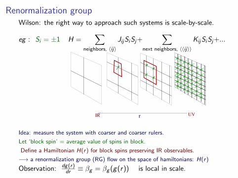
Renormalization groupWilson: the right way to approach such systems is scale-by-scale.

eg : Si = ±1 H =∑

neighbors, 〈ij〉

Jij Si Sj +∑

next neighbors, 〈〈ij〉〉

Kij Si Sj +...

IR rIR UV

Idea: measure the system with coarser and coarser rulers.

Let ‘block spin’ = average value of spins in block.

Define a Hamiltonian H(r) for block spins preserving IR observables.

−→ a renormalization group (RG) flow on the space of hamiltonians: H(r)

Observation: dg(r)dr ≡ βg = βg (g(r)) is local in scale.

RG fixed points give universal physics

H(water molecules)

H(IR fixed point)

UV

IR

r

H(electron spins in a ferromagnet)

J13

12

KUniversality: fixed points are rare.

Many microscopic theories willflow to the same fixed-point.

=⇒ same critical exponents.

The fixed point theory isscale-invariant (self-similar):if you change your resolution you get the

same picture back.

Often the fixed point theory is also‘Conformally invariant’.This is the ‘C’ in AdS/CFT.

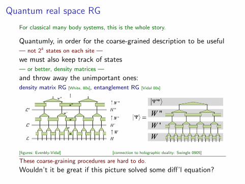
Quantum real space RG

For classical many body systems, this is the whole story.

Quantumly, in order for the coarse-grained description to be useful— not 2k states on each site —

we must also keep track of states— or better, density matrices —

and throw away the unimportant ones:density matrix RG [White, 80s], entanglement RG [Vidal 00s]

[figures: Evenbly-Vidal] [connection to holographic duality: Swingle 0905]

These coarse-graining procedures are hard to do.

Wouldn’t it be great if this picture solved some diff’l equation?

A theory of gravity is not like this.

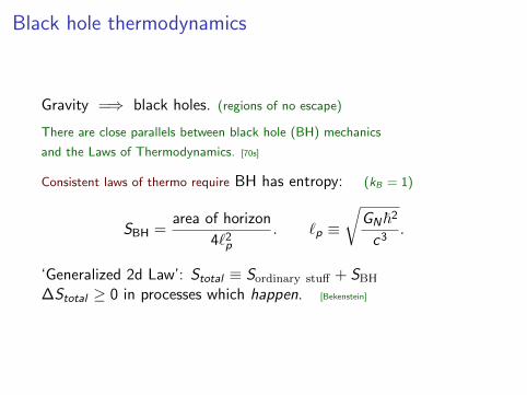
Black hole thermodynamics

Gravity =⇒ black holes. (regions of no escape)

There are close parallels between black hole (BH) mechanics

and the Laws of Thermodynamics. [70s]

Consistent laws of thermo require BH has entropy: (kB = 1)

SBH =area of horizon

4`2p

. `p ≡√

GN~2

c3.

‘Generalized 2d Law’: Stotal ≡ Sordinary stuff + SBH

∆Stotal ≥ 0 in processes which happen. [Bekenstein]

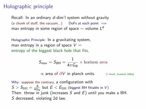
Holographic principle

Recall: In an ordinary d-dim’l system without gravity(a chunk of stuff, the vacuum...) DoFs at each point =⇒max entropy in some region of space ∼ volume Ld

Holographic Principle: In a gravitating system,max entropy in a region of space V =entropy of the biggest black hole that fits.

Smax = SBH =1

4πGN× horizon area

∝ area of ∂V in planck units. [’t Hooft, Susskind 1990s]

Why: suppose the contrary, a configuration withS > SBH = A

4GNbut E < EBH (biggest BH fittable in V )

Then: throw in junk (increases S and E ) until you make a BH.S decreased, violating 2d law.

Punchline: Gravity in d + 1 dimensions

has the same number of degrees of freedom as

a QFT in fewer (d) dimensions.

[Blundell2]

Questions:

• Who is the QFT on the boundary?• From its point of view, what is the extra dimension?• Where do I put the boundary?

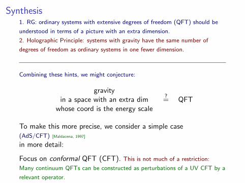
Synthesis1. RG: ordinary systems with extensive degrees of freedom (QFT) should be

understood in terms of a picture with an extra dimension.

2. Holographic Principle: systems with gravity have the same number of

degrees of freedom as ordinary systems in one fewer dimension.

Combining these hints, we might conjecture:

gravityin a space with an extra dim

whose coord is the energy scale

?= QFT

To make this more precise, we consider a simple case(AdS/CFT) [Maldacena, 1997]

in more detail:

Focus on conformal QFT (CFT). This is not much of a restriction:

Many continuum QFTs can be constructed as perturbations of a UV CFT by a

relevant operator.

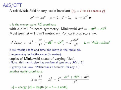
AdS/CFTA relativistic field theory, scale invariant (βg = 0 for all nonzero g)

xµ → λxµ µ = 0...d − 1, u → λ−1u

u is the energy scale, RG coordinate

with d-dim’l Poincare symmetry: Minkowski ds2 = −dt2 + d~x2

Most gen’l d + 1 dim’l metric w/ Poincare plus scale inv.

AdSd+1 : ds2 =u2

L2

(−dt2 + d~x2

)+ L2 du2

u2L ≡ ‘AdS radius′

If we rescale space and time and move in the radial dir,

the geometry looks the same (isometry).

copies of Minkowski space of varying ‘size’.(Note: this metric also has conformal symmetry SO(d , 2)

∃ gravity dual =⇒ “Polchinski’s Theorem” for any d .)

another useful coordinate:

z ≡ L2

uds2 = L2−dt2 + d~x2 + dz2

z2

[u] = energy, [z] = length (c = ~ = 1 units).

Geometry of AdS continued

uIR

R

AdSd+1

d−1,1

minkowski

UV

...

BOUNDARY

IR UVu

The extra (‘radial’) dimension is the resolution scale.(The bulk picture is a hologram.)

preliminary conjecture:

gravity on AdSd+1 space?= CFTd

crucial refinement:in a gravity theory the metric fluctuates.−→ what does ‘gravity in AdS’ mean ?!?

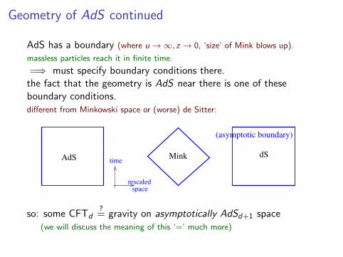
Geometry of AdS continued

AdS has a boundary (where u →∞, z → 0, ‘size’ of Mink blows up).

massless particles reach it in finite time.

=⇒ must specify boundary conditions there.the fact that the geometry is AdS near there is one of theseboundary conditions.different from Minkowski space or (worse) de Sitter:

AdS dSMink

(asymptotic boundary)

time

rescaledspace

so: some CFTd?= gravity on asymptotically AdSd+1 space

(we will discuss the meaning of this ‘=’ much more)

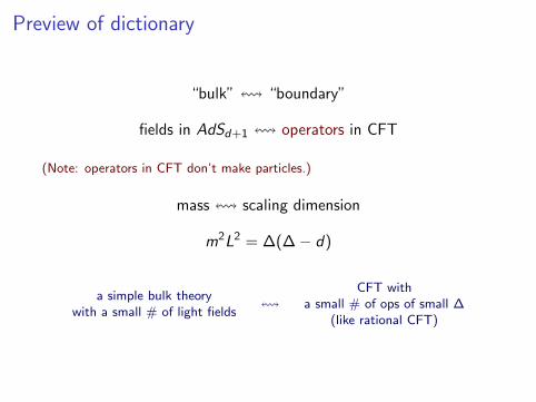
Preview of dictionary

“bulk” ! “boundary”

fields in AdSd+1 ! operators in CFT

(Note: operators in CFT don’t make particles.)

mass ! scaling dimension

m2L2 = ∆(∆− d)

a simple bulk theorywith a small # of light fields

!CFT with

a small # of ops of small ∆(like rational CFT)

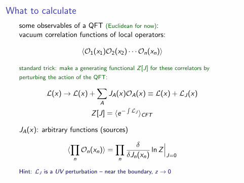
What to calculate

some observables of a QFT (Euclidean for now):vacuum correlation functions of local operators:

〈O1(x1)O2(x2) · · · On(xn)〉

standard trick: make a generating functional Z [J] for these correlators by

perturbing the action of the QFT:

L(x)→ L(x) +∑

A

JA(x)OA(x) ≡ L(x) + LJ(x)

Z [J] = 〈e−∫LJ 〉CFT

JA(x): arbitrary functions (sources)

〈∏

n

On(xn)〉 =∏

n

δ

δJn(xn)ln Z

∣∣∣J=0

Hint: LJ is a UV perturbation – near the boundary, z → 0

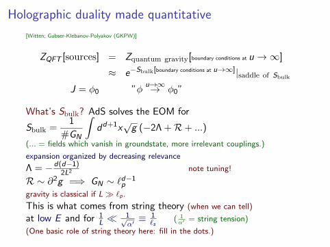
Holographic duality made quantitative

[Witten; Gubser-Klebanov-Polyakov (GKPW)]

ZQFT [sources] = Zquantum gravity[boundary conditions at u →∞]

≈ e−Sbulk[boundary conditions at u→∞]|saddle of Sbulk

J = φ0 ”φu→∞→ φ0”

What’s Sbulk? AdS solves the EOM for

Sbulk =1

#GN

∫dd+1x

√g (−2Λ +R+ ...)

(... = fields which vanish in groundstate, more irrelevant couplings.)

expansion organized by decreasing relevance

Λ = −d(d−1)2L2 note tuning!

R ∼ ∂2g =⇒ GN ∼ `d−1p

gravity is classical if L� `p.

This is what comes from string theory (when we can tell)

at low E and for 1L �

1√α′≡ 1

`s( 1α′ = string tension)

(One basic role of string theory here: fill in the dots.)

Conservation of evil

large AdS radius L ! strong coupling of QFT

(avoids an immediate disproof – obviously a perturbative QFT isn’t usefully an

extra-dimensional theory of gravity.)

a special case of a

Useful principle (Conservation of evil):different weakly-coupled descriptionshave non-overlapping regimes of validity.

strong/weak duality: hard to check, very powerfulInfo goes both ways: once we believe the duality, this is our best definition of

string theory.

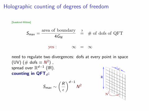
Holographic counting of degrees of freedom

[Susskind-Witten]

Smax =area of boundary

4GN

?= # of dofs of QFT

yes : ∞ = ∞

need to regulate two divergences: dofs at every point in space(UV) (# dofs ≡ N2) ,spread over Rd−1 (IR).

2

R

ε

N

counting in QFTd :

Smax ∼(

R

ε

)d−1

N2

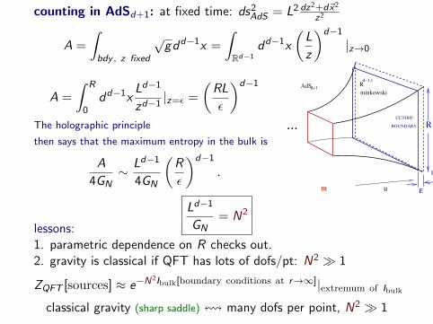
counting in AdSd+1: at fixed time: ds2AdS = L2 dz2+d~x2

z2

A =

∫bdy , z fixed

√gdd−1x =

∫Rd−1

dd−1x

(L

z

)d−1

|z→0

R

IR

AdSd+1

u

UV

d−1,1

minkowski

...

ε

RACTUAL

BOUNDARYBOUNDARY

CUTOFF

A =

∫ R

0dd−1x

Ld−1

zd−1|z=ε =

(RL

ε

)d−1

The holographic principle

then says that the maximum entropy in the bulk is

A

4GN∼ Ld−1

4GN

(R

ε

)d−1

.

Ld−1

GN= N2

lessons:1. parametric dependence on R checks out.2. gravity is classical if QFT has lots of dofs/pt: N2 � 1

ZQFT [sources] ≈ e−N2Ibulk[boundary conditions at r→∞]|extremum of Ibulk

classical gravity (sharp saddle) ! many dofs per point, N2 � 1

A word about large N2

Most prominent example: ’t Hooft limit of N × N matrix fields X .Physical operators are Ok = tr X k

This accomplishes several related things:

• 〈OO〉 ∼ 〈O〉〈O〉+ o(N−2

)is the statement that something (the excitations created by O) behavesclassically.• provides notion of single-particle states in bulk.• makes saddle well-peaked Z ∼ e−N2I

comments:• This is different from a vector-like large-N limit, where the fields are vectors

with N components. In that case, QFT techniques are more useful (fewer

diagrams) and holographic duality (higher spins) is less useful.• this is just the best-understood class of examples.in other examples, the # of dofs goes like Nb, b 6= 2.

I’ll always write N2 as a proxy for this large number.

Recap

gravity in spacetimesd+1

with timelike asymptotic boundaries! QFTd

important special case:

gravity in AdSd+1 = d-dimensional conformal field theory (CFT)isometries of AdSd+1 ! conformal symmetry

AdS : ds2 =r 2

R2

(−dt2 + d~x2

)+ R2 dr 2

r 2

IR UVu

R

d+1

d−1,1

Minkowski

UV

IR r

AdS

...

BOUNDARY

The extra (‘radial’) dimension r = 1/z is the resolution scale.

fields in bulk ! (possibly-) running couplings

ZQFT [sources, φ0] ≈ e−N2Ibulk[boundary conditions at r→∞]|saddle of Ibulk

More of the dictionaryreally a φa for every Oa in CFT. how to match?

1. organize into reps of conformal group2. single-trace operators correspond to ‘elementary fields’ in the bulk.

states from multitrace ops (tr X k )2|0〉 — 2-particle states of φ.

3. simple egs fixed by symmetry:• gauge fields in bulk Aµ – global currents Jµ in bdy

SQFT 3∫

AµJµ (massless A! conserved J)

• def of QFT stress tensor: response to change in metric onboundary SQFT 3

∫δgµνTµν

energy momentum tensor: Tµν

global current: Jµ

scalar operator: OB

fermionic operator: OF

!

graviton: gab

Maxwell field: Aa

scalar field: φfermionic field: ψ .

boundary conditions on bulk fields ! couplings in field theorye.g.: boundary value of bulk metric limr→∞ gµν

= source for stress-energy tensor Tµν

different couplings in bulk action ! different field theories

Next: a few technical slides from which we can confirm ourinterpretation

u = RG scale

and see the machinery at work.

How to calculate

ZQFT [sources] ≈ e−N2Ibulk[boundary conditions at z→0]|extremum of Ibulk

more explicitly:

ZQFT [sources, φ0] ≡ 〈e−∫φ0O〉CFT

≈ e−N2Ibulk[φ|φ(z=ε)?=φ0]|φ solves EOM of Ibulk

As when counting dofs, we anticipate UV divergencesat the boundary z → 0,cut off the bulk at z = εand set bc’s there. R

IR

AdSd+1

u

UV

d−1,1

minkowski

...

ε

RACTUAL

BOUNDARYBOUNDARY

CUTOFF

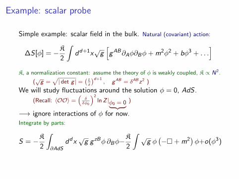
Example: scalar probe

Simple example: scalar field in the bulk. Natural (covariant) action:

∆S [φ] = −K

2

∫dd+1x

√g[g AB∂Aφ∂Bφ+ m2φ2 + bφ3 + . . .

]K, a normalization constant: assume the theory of φ is weakly coupled, K ∝ N2.

(√g =

√| det g | =

(Lz

)d+1, gAB = δABz2 )

We will study fluctuations around the solution φ = 0, AdS .

(Recall: 〈OO〉 =(

δδφ0

)2

lnZ |φ0 = 0︸ ︷︷ ︸ )

−→ ignore interactions of φ for now.Integrate by parts:

S = −K

2

∫∂AdS

dd x√

g g zBφ∂Bφ−K

2

∫ √g φ(−�+ m2

)φ+o(φ3)

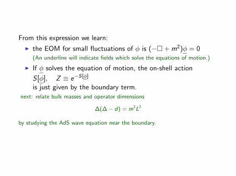
From this expression we learn:

I the EOM for small fluctuations of φ is (−�+ m2)φ = 0(An underline will indicate fields which solve the equations of motion.)

I If φ solves the equation of motion, the on-shell action

S [φ], Z ≡ e−S[φ]

is just given by the boundary term.

next: relate bulk masses and operator dimensions

∆(∆− d) = m2L2

by studying the AdS wave equation near the boundary.

Wave equation in AdStranslational invariance in d dimensions, xµ → xµ + aµ,

Fourier : φ(z , xµ) = e ikµxµfk (z), kµxµ ≡ −ωt + ~k · ~x

0 = (gµνkµkν −1√

g∂z (√

gg zz∂z ) + m2)fk (z)

=1

L2[z2k2 − zd+1∂z (z−d+1∂z ) + m2L2]fk (z), (1)

we used gAB = (z/L)2δAB ,√g =

√| det g | =

(Lz

)d+1.

Near boundary (z → 0), power law solns, (spoiled by the z2k2 term).Try fk = z∆ in (1):

0 = k2z2+∆ − zd+1∂z (∆z−d+∆) + m2L2z∆

= (k2z2 −∆(∆− d) + m2L2)z∆,

and for z → 0 we get:

∆(∆− d) = m2L2 (2)

The two roots of (2) are ∆± = d2 ±

√(d2

)2+ m2L2.

Comments

∆± = d2 ±

√(d2

)2+ m2L2.

-2.0 -1.5 -1.0 -0.5 0.5 1.0m

2

0.5

1.0

1.5

2.0

2.5

3.0

D

I The solution proportionalto z∆− is bigger near z → 0. →usually the source (‘non-normalizable’)

I ∆+ > 0 ∀ m: z∆+ always decays nearthe boundary

I ∆+ + ∆− = d .

We want to impose boundary conditions that allow solutions.Leading z → 0 behavior of generic solution: φ ∼ z∆− , we impose

φ(x , z)|z=ε!

= φ0(x , ε) = ε∆−φRen0 (x),

where φRen0 is a renormalized source field.

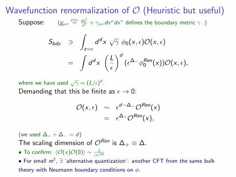
Wavefunction renormalization of O (Heuristic but useful)Suppose: (gµν

z≈ε= dz2

z2 + γµνdxµdxν defines the boundary metric γ .)

Sbdy 3∫

z=εdd x

√γ φ0(x , ε)O(x , ε)

=

∫dd x

(L

ε

)d

(ε∆−φRen0 (x))O(x , ε),

where we have used√γ = (L/ε)d .

Demanding that this be finite as ε→ 0:

O(x , ε) ∼ εd−∆−ORen(x)

= ε∆+ORen(x),

(we used ∆+ + ∆− = d)

The scaling dimension of ORen is ∆+ ≡ ∆.• To confirm: 〈O(x)O(0)〉 ∼ 1

|x|2∆

• For small m2, ∃ ‘alternative quantization’: another CFT from the same bulk

theory with Neumann boundary conditions on φ.

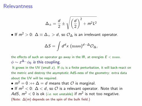
Relevantness

∆± =d

2±

√(d

2

)2

+ m2L2

• If m2 > 0: ∆ ≡ ∆+ > d , so O∆ is an irrelevant operator.

∆S =

∫dd x (mass)d−∆O∆,

the effects of such an operator go away in the IR, at energies E < mass.

φ ∼ z∆−φ0 is this coupling.It grows in the UV (small z). If φ0 is a finite perturbation, it will back-react on

the metric and destroy the asymptotic AdS-ness of the geometry: extra data

about the UV will be required.

• m2 = 0 :↔ ∆ = d means that O is marginal.• If m2 < 0: ∆ < d , so O is a relevant operator. Note that inAdS , m2 < 0 is ok (i.e. not unstable) if m2 is not too negative.(Note: ∆(m) depends on the spin of the bulk field.)

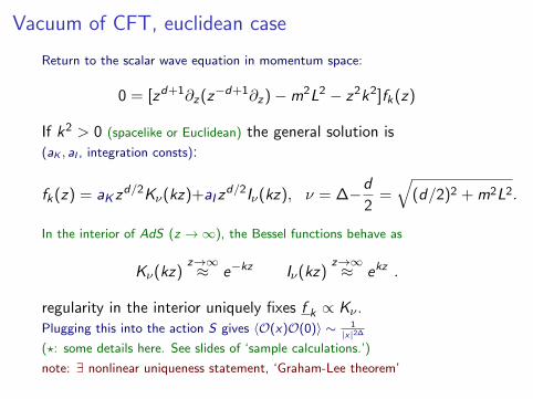
Vacuum of CFT, euclidean case

Return to the scalar wave equation in momentum space:

0 = [zd+1∂z (z−d+1∂z )−m2L2 − z2k2]fk (z)

If k2 > 0 (spacelike or Euclidean) the general solution is(aK , aI , integration consts):

fk (z) = aK zd/2Kν(kz)+aI zd/2Iν(kz), ν = ∆−d

2=√

(d/2)2 + m2L2.

In the interior of AdS (z →∞), the Bessel functions behave as

Kν(kz)z→∞≈ e−kz Iν(kz)

z→∞≈ ekz .

regularity in the interior uniquely fixes f k ∝ Kν .Plugging this into the action S gives 〈O(x)O(0)〉 ∼ 1

|x|2∆

(?: some details here. See slides of ‘sample calculations.’)

note: ∃ nonlinear uniqueness statement, ‘Graham-Lee theorem’

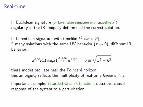
Real-time

In Euclidean signature (or Lorentzian signature with spacelike k2)

regularity in the IR uniquely determined the correct solution.

In Lorentzian signature with timelike k2 (ω2 > ~k2),∃ many solutions with the same UV behavior (z → 0), different IRbehavior:

zd/2Kν(±iqz)z→∞≈ e±iqz q ≡

√ω2 − ~k2

these modes oscillate near the Poincare horizon.this ambiguity reflects the multiplicity of real-time Green’s f’ns.

Important example: retarded Green’s function, describes causalresponse of the system to a perturbation.

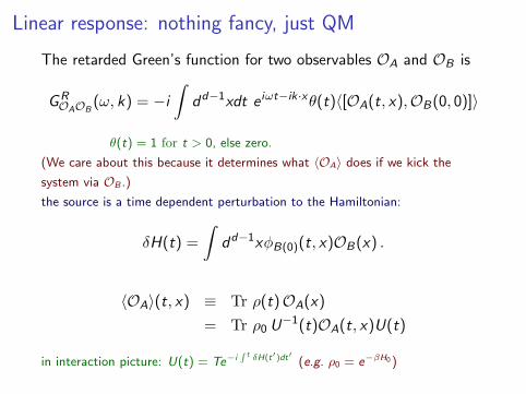
Linear response: nothing fancy, just QM

The retarded Green’s function for two observables OA and OB is

G ROAOB

(ω, k) = −i

∫dd−1xdt e iωt−ik·xθ(t)〈[OA(t, x),OB(0, 0)]〉

θ(t) = 1 for t > 0, else zero.

(We care about this because it determines what 〈OA〉 does if we kick the

system via OB .)

the source is a time dependent perturbation to the Hamiltonian:

δH(t) =

∫dd−1xφB(0)(t, x)OB(x) .

〈OA〉(t, x) ≡ Tr ρ(t)OA(x)

= Tr ρ0 U−1(t)OA(t, x)U(t)

in interaction picture: U(t) = Te−i∫ t δH(t′)dt′ (e.g. ρ0 = e−βH0 )

Linear response, cont’d

linearize in small perturbation:

δ〈OA〉(t, x) = −iTr ρ0

∫ t

dt ′[OA(t, x), δH(t ′)]

= −i

∫ t

dd−1x ′dt ′〈[OA(t, x),OB(t ′, x ′)]〉φB(0)(t ′, x ′)

=

∫dx ′GR(x , x ′)φB(x ′)

fourier transform:

δ〈OA〉(ω, k) = G ROAOB

(ω, k)δφB(0)(ω, k)

Linear response, an example

perturbation: an external electric field, Ex = iωAx

couples via δH = Ax Jx where J is the electric current (OB = Jx )

response: the electric current (OA = Jx )

δ〈OA〉(ω, k) = G ROAOB

(ω, k)δφB(0)(ω, k)

it’s safe to assume 〈J〉E=0 = 0:

〈OJ〉(ω, k) = G RJJ(ω, k)Ax = G R

JJ(ω, k)Ex

iω

Ohm’s law: J = σE

=⇒ Kubo formula : σ(ω, k) =G R

JJ(ω, k)

iω

Holographic real-time prescription

Claim [Son-Starinets 2002]: to compute GR , take the solution which atz →∞ describes stuff falling into the horizon

I Both the retarded response and stuff falling through thehorizon describe things that happen, rather than unhappen.

I You can check that this prescription gives the correct analyticstructure of GR(ω) ([Son-Starinets] and all the hundreds of papers that

have used this prescription).

I It has been derived from a holographic version of theSchwinger-Keldysh prescription [Herzog-Son, Maldacena, Skenderis-van Rees].

The fact that stuff goes past the horizon and doesn’t come out is what breaks

time-reversal invariance in the holographic computation of GR .

For a scalar in empty AdS the ingoing choice is φ(t, z) ∼ e−iωt+iqz :as t grows, the wavefront moves to larger z .

(the solution which computes causal response is zd/2K+ν(iqz).)

The same prescription, adapted to the black hole horizon, works inthe finite temperature case.

What to do with the solution

determining 〈OO〉 is like a scattering problem in QM

The solution of the equations of motion, satisfying the desired IR bc,behaves near the boundary as

φ(z , x) ≈(z

L

)∆−φ0(x)

(1 +O(z2)

)+(z

L

)∆+

φ1(x)(1 +O(z2)

);

this formula defines the coefficient φ1 of the subleading behavior of the solution.

All the information about G is in φ0, φ1.

recall: Z [φ0] ≡ e−W [φ0] ' e−Sbulk[φ]|φ

z→0→ z∆−φ0confession: this is a euclidean eqn. next: a nice general trick. [Iqbal-Liu]

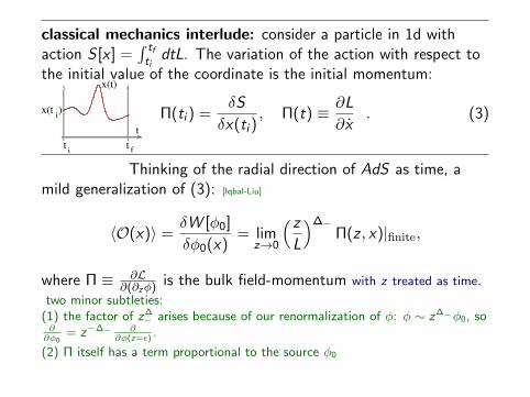
classical mechanics interlude: consider a particle in 1d withaction S [x ] =

∫ tf

tidtL. The variation of the action with respect to

the initial value of the coordinate is the initial momentum:

Π(ti ) =δS

δx(ti ), Π(t) ≡ ∂L

∂x. (3)

f

x(t)

ti

x(t )i

t

t

Thinking of the radial direction of AdS as time, amild generalization of (3): [Iqbal-Liu]

〈O(x)〉 =δW [φ0]

δφ0(x)= lim

z→0

(z

L

)∆−Π(z , x)|finite,

where Π ≡ ∂L∂(∂zφ) is the bulk field-momentum with z treated as time.

two minor subtleties:(1) the factor of z∆

− arises because of our renormalization of φ: φ ∼ z∆−φ0, so∂∂φ0

= z−∆− ∂∂φ(z=ε)

.

(2) Π itself has a term proportional to the source φ0

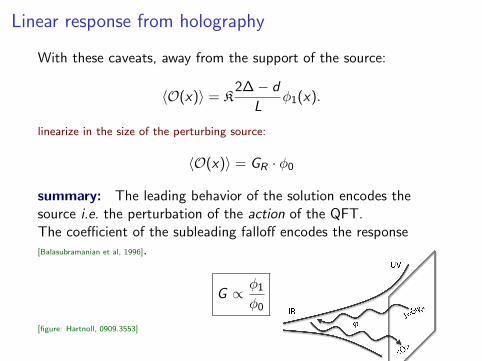
Linear response from holography

With these caveats, away from the support of the source:

〈O(x)〉 = K2∆− d

Lφ1(x).

linearize in the size of the perturbing source:

〈O(x)〉 = GR · φ0

summary: The leading behavior of the solution encodes thesource i.e. the perturbation of the action of the QFT.The coefficient of the subleading falloff encodes the response[Balasubramanian et al, 1996].

G ∝ φ1

φ0

[figure: Hartnoll, 0909.3553]

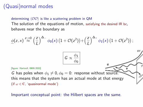
(Quasi)normal modes

determining 〈OO〉 is like a scattering problem in QM

The solution of the equations of motion, satisfying the desired IR bc,behaves near the boundary as

φ(z , x)z→0≈(z

L

)∆−φ0(x)

(1 +O(z2)

)+(z

L

)∆+

φ1(x)(1 +O(z2)

);

G ∝ φ1

φ0

[figure: Hartnoll, 0909.3553]

G has poles when φ1 6= 0, φ0 = 0: response without source.this means that the system has an actual mode at that energy(if ω ∈C, ‘quasinormal mode’)

Important conceptual point: the Hilbert spaces are the same.

Next: thermal equilibrium

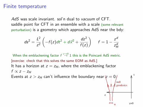
Finite temperature

AdS was scale invariant. sol’n dual to vacuum of CFT.saddle point for CFT in an ensemble with a scale (some relevant

perturbation) is a geometry which approaches AdS near the bdy:

ds2 =L2

z2

(−f (z)dt2 + d~x2 +

dz2

f (z)

)f = 1− zd

zdH

When the emblackening factor fz→0→ 1 this is the Poincare AdS metric.

[exercise: check that this solves the same EOM as AdS.]

It has a horizon at z = zH , where the emblackening factorf ∝ z − zH

Events at z > zH can’t influence the boundary near z = 0:

z=0

t

null

geodesics

z

z=zH

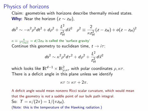
Physics of horizonsClaim: geometries with horizons describe thermally mixed states.Why: Near the horizon (z ∼ zH),

ds2 ∼ −κ2ρ2dt2 + dρ2 +L2

z2H

d~x2 ρ2 ≡ 2

κz2H

(z − zH) + o(z − zH)2

κ ≡ 4|f ′(zH )| = d/2zH is called the ‘surface gravity’

Continue this geometry to euclidean time, t → iτ :

ds2 ∼ κ2ρ2dτ2 + dρ2 +L2

z2H

d~x2

which looks like IRd−1 × IR2ρ,κτ with polar coordinates ρ, κτ .

There is a deficit angle in this plane unless we identify

κτ ' κτ + 2π.

A deficit angle would mean nonzero Ricci scalar curvature, which would mean

that the geometry is not a saddle point of our bulk path integral.

So: T = κ/(2π) = 1/(πzH).(Note: this is the temperature of the Hawking radiation.)

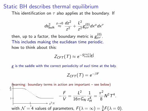
Static BH describes thermal equilibriumThis identification on τ also applies at the boundary. If

ds2bulk

z→0≈ dz2

z2+

L2

z2g (0)µν dxµdxν

then, up to a factor, the boundary metric is g(0)µν .

This includes making the euclidean time periodic.how to think about this:

ZCFT (T ) ≈ e−Seuclbulk[g ]

g is the saddle with the correct periodicity of eucl time at the bdy.

ZCFT (T ) = e−βF

(warning: boundary terms in action are important – see below)

− F

V=

L2

16πGN

1

z4H

=π2

8N2T 4.

with N = 4 values of parameters, F (λ =∞) = 34 F (λ = 0).

g2N

1

1

43π2

2N2T 3V

S

QFT thermodynamics from black holes cont’dThe Bekenstein-Hawking entropy is

S =A

4GN=

Ld−1

4GN

V

zd−1H

=N2

2π(πT )d−1V =

π2

2N2VT d−1 .

The Bekenstein-Hawking entropy density is

sBH =SBH

V=

aBH

4GN.

where aBH ≡ AV is the ‘area density’ of the black hole.

checks:

• SBH

horizon

= − ∂F∂T

integral over all spacetime

(That is, the first law of thermo holds.)

• cV > 0 for AdS BH. (unlike schwarzchild in asymptotically flat space!)

• uniqueness of stationary BH(‘no hair’)

!few state variables

in eq thermo

Next: deviations from thermal equilibrium

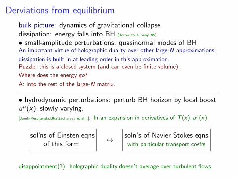
Derviations from equilibrium

bulk picture: dynamics of gravitational collapse.dissipation: energy falls into BH [Horowitz-Hubeny, 99]

• small-amplitude perturbations: quasinormal modes of BHAn important virtue of holographic duality over other large-N approximations:

dissipation is built in at leading order in this approximation.Puzzle: this is a closed system (and can even be finite volume).

Where does the energy go?

A: into the rest of the large-N matrix.

• hydrodynamic perturbations: perturb BH horizon by local boostuµ(x), slowly varying.[Janik-Peschanski,Bhattacharyya et al...]: In an expansion in derivatives of T (x), uµ(x),

sol’ns of Einsten eqnsof this form

↔ soln’s of Navier-Stokes eqnswith particular transport coeffs

disappointment(?): holographic duality doesn’t average over turbulent flows.

Derviations from equilibrium, cont’d

• far-from equilibrium processes: [Chesler-Yaffe 08] (PDEs!)

input: -3 -2 -1 1 2 3Τ

1.0

1.2

1.4

gxxHΤL

output:

black hole forms from vacuum initial conditions.

brutally brief summary: all relaxation timescales τth ∼ T−1.

More recently: ‘turbulent’ bulksolutions [Adams-Chesler-Liu 13]

(not obviously in hydro regime)

End of first lecture (I hope).

Appendices

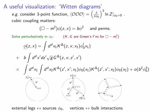
A useful visualization: ‘Witten diagrams’e.g. consider 3-point function, 〈OOO〉 =

(δδφ0

)3ln Z |φ0=0 .

cubic coupling matters:

(�−m2)φ(z , x) = bφ2 and perms.

Solve perturbatively in φ0: (K ,G are Green’s f’ns for �−m2i )

φ(z , x) =

∫dd x1K ∆(z , x ; x1)φ

(0x1)

+ b

∫dd x ′dz ′

√gG ∆(z , x ; z ′, x ′)

×∫

dd x1

∫dd x2K ∆(z ′, x ′; x1)φ0(x1)K ∆(z ′, x ′; x2)φ0(x2) + o(b2φ3

0)

(x )iφ0 1

K

(z,x)

i

φ0

φ0(x )

2

k

(z’,x’)

K

K

Gi

k

j

(x )1

(z,x)

j

external legs ↔ sources φ0, vertices ↔ bulk interactions

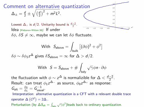
Comment on alternative quantization∆± = d

2 ±√(

d2

)2+ m2L2.

-2.0 -1.5 -1.0 -0.5 0.5 1.0m

2

0.5

1.0

1.5

2.0

2.5

3.0

D

Lowest ∆+ is d/2. Unitarity bound is d−22

.

Idea [Klebanov-Witten 99]: If underδφ, δS 6=∞, maybe we can let δφ fluctuate.

With Sabove =

∫bulk

[(∂φ)2 + φ2

]δφ ∼ δφ1z∆ gives δSabove =∞ for ∆ > d/2.

With S = Sabove + #

∫bdy

√γφn · ∂φ

the fluctuation with φ ∼ z∆ is normalizible for ∆ < d−22 .

Result: can treat φ1z∆− as source, φ0z∆+ as response:Galt = φ0

φ1= G−1

usual.Interpretation: alternative quantization is a CFT with a relevant double trace

operator ∆(O2)

= 2∆−

Perturbation (by ∆Salt =∫

bdy

√γφ2)leads back to ordinary quantization.

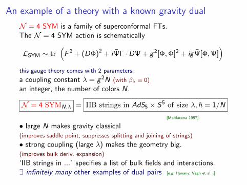
An example of a theory with a known gravity dual

N = 4 SYM is a family of superconformal FTs.The N = 4 SYM action is schematically

LSYM ∼ tr(

F 2 + (DΦ)2 + iΨΓ · DΨ + g 2[Φ,Φ]2 + igΨ[Φ,Ψ])

this gauge theory comes with 2 parameters:

a coupling constant λ = g 2N (with βλ ≡ 0)

an integer, the number of colors N.

N = 4 SYMN,λ = IIB strings in AdS5 × S5 of size λ, ~ = 1/N

[Maldacena 1997]

• large N makes gravity classical(improves saddle point, suppresses splitting and joining of strings)

• strong coupling (large λ) makes the geometry big.(improves bulk deriv. expansion)

‘IIB strings in ...’ specifies a list of bulk fields and interactions.∃ infinitely many other examples of dual pairs [e.g. Hanany, Vegh et al...]

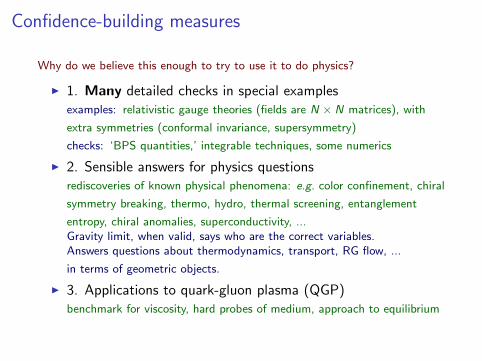
Confidence-building measures

Why do we believe this enough to try to use it to do physics?

I 1. Many detailed checks in special examplesexamples: relativistic gauge theories (fields are N × N matrices), with

extra symmetries (conformal invariance, supersymmetry)

checks: ‘BPS quantities,’ integrable techniques, some numerics

I 2. Sensible answers for physics questionsrediscoveries of known physical phenomena: e.g. color confinement, chiral

symmetry breaking, thermo, hydro, thermal screening, entanglement

entropy, chiral anomalies, superconductivity, ...Gravity limit, when valid, says who are the correct variables.Answers questions about thermodynamics, transport, RG flow, ...

in terms of geometric objects.

I 3. Applications to quark-gluon plasma (QGP)benchmark for viscosity, hard probes of medium, approach to equilibrium

Appendix:

Counting powers of N2

large N counting

consider a matrix field theoryΦb

a is a matrix field. a, b = 1..N. other labels (e.g. spatial position,

spin) are suppressed.

L ∼ 1

g 2Tr((∂Φ)2 + Φ2 + Φ3 + Φ4 + . . .

)here e.g. (Φ2)c

a = ΦbaΦc

b,the interactions are invariant under the U(N) symmetryΦ→ U−1ΦU

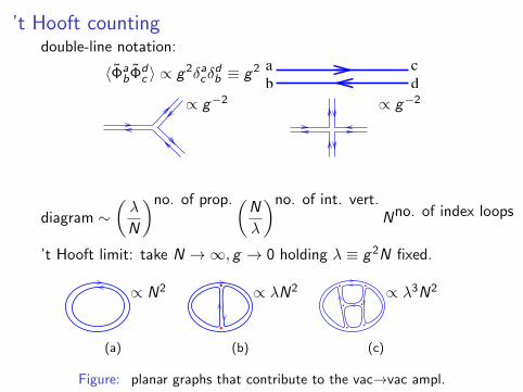
’t Hooft countingdouble-line notation:

〈ΦabΦd

c 〉 ∝ g 2δacδ

db ≡ g 2

d

a

b

c

∝ g−2 ∝ g−2

diagram ∼(λ

N

)no. of prop.(N

λ

)no. of int. vert.Nno. of index loops

’t Hooft limit: take N →∞, g → 0 holding λ ≡ g 2N fixed.

∝ N2

(a)

b

b

∝ λN2

(b)

bb

b b

bb

∝ λ3N2

(c)

Figure: planar graphs that contribute to the vac→vac ampl.

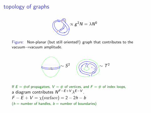
topology of graphs

b

b

∝ g 2N = λN0

Figure: Non-planar (but still oriented!) graph that contributes to thevacuum→vacuum amplitude.

∼ S2 ∼ T 2

If E = #of propagators, V = # of vertices, and F = # of index loops,

a diagram contributes NF−E+VλE−V .F − E + V = χ(surface) = 2− 2h − b(h = number of handles, b = number of boundaries)

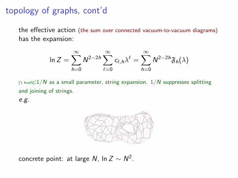
topology of graphs, cont’d

the effective action (the sum over connected vacuum-to-vacuum diagrams)

has the expansion:

ln Z =∞∑

h=0

N2−2h∞∑`=0

c`,hλ` =

∞∑h=0

N2−2hFh(λ)

[’t hooft]:1/N as a small parameter, string expansion. 1/N suppresses splitting

and joining of strings.

e.g.

concrete point: at large N, ln Z ∼ N2.

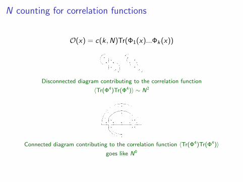
N counting for correlation functions

O(x) = c(k ,N)Tr(Φ1(x)...Φk (x))

Disconnected diagram contributing to the correlation function

〈Tr(Φ4)Tr(Φ4)〉 ∼ N2

Connected diagram contributing to the correlation function 〈Tr(Φ4)Tr(Φ4)〉goes like N0