Holographic studies of Einsteinian cubic gravity

Pablo Bueno,a Pablo A. Canob,c and Alejandro Ruipérezb

aInstituut voor Theoretische Fysica, KU Leuven,Celestijnenlaan 200D, B-3001 Leuven, BelgiumbInstituto de Física Teórica UAM/CSIC,C/ Nicolás Cabrera, 13-15, C.U. Cantoblanco, 28049 Madrid, SpaincPerimeter Institute for Theoretical Physics,Waterloo, ON N2L 2Y5, Canada

Abstract: Einsteinian cubic gravity provides a holographic toy model of a nonsupersym-metric CFT in three dimensions, analogous to the one defined by Quasi-topological gravityin four. The theory admits explicit non-hairy AdS4 black holes and allows for numerous ex-act calculations, fully nonperturbative in the new coupling. We identify several entries ofthe AdS/CFT dictionary for this theory, and study its thermodynamic phase space, findinginteresting new phenomena. We also analyze the dependence of Rényi entropies for disk re-gions on universal quantities characterizing the CFT. In addition, we show that η/s is givenby a non-analytic function of the ECG coupling, and that the existence of positive-energyblack holes strictly forbids violations of the KSS bound. Along the way, we introduce a newmethod for evaluating Euclidean on-shell actions for general higher-order gravities possess-ing second-order linearized equations on AdS(d+1). Our generalized action involves the verysame Gibbons-Hawking boundary term and counterterms valid for Einstein gravity, whichnow appear weighted by the universal charge a∗ controlling the entanglement entropy acrossa spherical region in the CFT dual to the corresponding higher-order theory.

arX

iv:1

802.

0001

8v3

[he

p-th

] 2

8 M

ar 2

018

Contents

1 Introduction 21.1 Summary of results 3

2 Einsteinian cubic gravity 52.1 AdS4 vacua and linearized spectrum 7

3 AdS4 black holes 93.1 Asymptotic expansion 103.2 Near-horizon expansion 113.3 Full solutions 12

4 Generalized action for higher-order gravities 144.1 a∗ and generalized action 174.2 Generalized action for Quasi-topological gravity 184.3 Generalized action for Einsteinian cubic gravity 19

5 Stress tensor two-point function charge CT 19

6 Thermodynamics 236.1 Entropy, energy and free energy 236.2 Thermal entropy charge CS 256.3 Toroidal boundary: black brane vs AdS4 soliton 266.4 Spherical boundary: Hawking-Page transitions 27

7 Rényi entropy 317.1 Holographic Rényi entropy 317.2 Scaling dimension of twist operators 377.3 Stress tensor three-point function charge t4 38

8 Holographic hydrodynamics 39

9 Final comments 449.1 Generalized action, a∗ and holographic complexity? 44

A 〈TTT 〉 parameters from hq 46A.1 Gauss-Bonnet in arbitrary dimensions 46A.2 Quasi-topological gravity 47

B Generalized action for Gauss-Bonnet gravity 48

– 1 –

C Boundary terms in the two-point function 50

1 Introduction

Higher-order gravities play an important role in AdS/CFT [1–3]. Perturbative correctionsto the large-N and strong-coupling limits of holographic CFTs are encoded, from the bulkperspective, in higher-curvature interactions which modify the semiclassical Einstein (su-per)gravity action — see e.g., [4–7]. The introduction of such terms, which is in principlefully controlled by String Theory, gives rise to holographic theories belonging to universalityclasses different from the one defined by Einstein gravity [8–10] — e.g., one can constructCFTs with a 6= c in d = 4 [11, 12]. Some care must be taken, however. As shown in [13],higher-curvature terms making finite contributions to physical quantities in the dual CFT canbecome acausal unless new higher-spin (J > 2) modes appear at the scale controlling thecouplings of such terms.

In spite of this, a great deal of non-trivial information can be still obtained by consider-ing particular higher-curvature interactions at finite coupling — i.e., beyond a perturbativeapproach. The idea is to select theories whose special properties make them amenable tocalculations — something highly nontrivial in general. The approach turns out to be veryrewarding and, in some cases, it has led to the discovery of universal properties valid forcompletely general CFTs [14–18]. In other cases, higher-order gravities have served as a proofof concept, e.g., providing counterexamples [7, 19–23] to the Kovtun-Son-Starinets bound forthe shear viscosity over entropy density ratio [24] — see discussion below. Just like free-fieldtheories, these holographic higher-order gravities should be regarded as toy models for whichmany calculations can be explicitly performed, hence providing important insights on physicalquantities otherwise practically inaccesible for most CFTs — see e.g., [25–28] for additionalexamples.

A key property one usually demands from a putative holographic model of this kind isthat it admits explicit AdS black-hole solutions. In d ≥ 4, this canonically selects Gauss-Bonnet or, more generally, Lovelock gravities [29, 30], for which numerous holographic studieshave been performed in different contexts — see e.g., [31–39] and references therein. Thenext-to-simplest example in d = 4 is Quasi-topological gravity (QTG) [40, 41], a theory whichincludes, in addition to the Einstein gravity and Gauss-Bonnet terms, an extra density, cubicin the Riemann tensor. Besides admitting simple generalizations of the Einstein gravity AdSblack holes, and having second-order linearized equations of motion on maximally symmetricbackgrounds, this theory contains three dimensionless parameters: the ratio of the cosmo-logical constant scale over the Newton constant, L2/G, and the new gravitational couplings,λ and µ. These can be translated into the three parameters characterizing the three-pointfunction of the boundary stress tensor. As opposed to Lovelock theories, for which one ofsuch parameters, customarily denoted t4 [9], is always zero [33–35, 42], the new QTG coupling

– 2 –

gives rise to a nonvanishing t4 [43]. For supersymmetric theories one also has t4 = 0 [9, 44],so QTG provides a toy model of a non-supersymmetric CFT in four dimensions.

All studies performed so far involving finite higher-curvature couplings have been re-stricted to d ≥ 4 — observe that all theories mentioned in the previous paragraph reduce toEinstein gravity for d = 3. Obviously, from the CFT side, there is no fundamental reason toexclude holographic three-dimensional theories. In fact, there exist many interesting CFTs ind = 3 with known holographic duals, e.g., [1, 45–49]. The actual reason for the absence ofholographic studies involving higher-curvature terms in d = 3 has been the lack of examplesadmitting generalizations of Einstein gravity black holes in four bulk dimensions. The situ-ation has recently changed thanks to the discovery of Einsteinian cubic gravity (ECG) [50],for which such generalizations are possible [51, 52] — see section 2 for a detailed review. Aswe show here, ECG provides a holographic toy model of a nonsupersymmetric CFT in threedimensions, analogous to the one defined by QTG in four. The main purpose of this paper isto study the behavior of several physical quantities in this new model. Just like it occurs forLovelock and QTG in d ≥ 4, all results can be obtained fully nonperturbatively in the newgravitational coupling, which provides a much better handle on the corresponding quantitiesthan any possible perturbative calculation.

On a more general front, we propose a new method for computing Euclidean on-shellactions for asymptotically AdS(d+1) solutions of an important class of general higher-ordergravities — those for which the linearized equations become second-order on maximally sym-metric backgrounds. Our generalized action represents a drastic simplification with respect tostandard approaches, as it utilizes the same boundary term and counterterms as for Einsteingravity, but weighted by a universal quantity related to the entanglement entropy across aspherical region in the boundary theory.

A more precise summary of our findings can be found next.

1.1 Summary of results

The paper is somewhat divided into two main parts. In the first, which includes sections2, 3 and 4, we develop some preliminary results and techniques which are necessary for theholographic computations which we perform in sections 5 to 8.

• In section 2, we start with a review of ECG and recent developments. Then, we char-acterize the AdS4 vacua of the theory, and identify the range of (in principle) allowedvalues of the new coupling and its relation to the existence of a critical limit for whichthe effective Newton constant blows up.

• In section 3, we construct the AdS4 black holes of ECG with general horizon topology.

• In section 4, we propose a new method for computing on-shell actions of asymptotically-AdS solutions of general higher-order gravities whose linearized spectrum on AdS(d+1)

matches that of Einstein gravity. We claim that the corresponding boundary termand counterterms can be chosen to be proportional to the usual Einstein gravity ones.

– 3 –

Amusingly, we find that the proportionality factor is controlled by the charge a∗ char-acterizing the entanglement entropy across a spherical region Sd−2 in the dual CFT.As a first consistency check of our proposal, we use our generalized action to prove therelation between a∗ and the on-shell gravitational Lagrangian L|AdS for odd-dimensionalholographic CFTs with higher-curvature duals.

• In section 5, we compute the charge CT controlling the correlator of the boundary stress-tensor from an explicit holographic computation and show that the result agrees withthe (not so) naive expectation obtained from the effective Newton constant. We arguethat the detailed cancellations between bulk and boundary contributions giving rise tothe correct answer constitute a strong check of the generalized action proposed in theprevious section.

• In section 6, we start with another check of our generalized action, consisting in anexplicit calculation of the free energy of ECG AdS4 black holes, which we show to agreewith the one obtained using Wald’s entropy approach. Then we compute the thermalentropy charge CS, and we note that it presents notable differences with respect toprevious results for other higher-curvature holographic models in d ≥ 4. Then, we studythe thermal phase space of holographic ECG with toroidal and spherical boundaries,respectively. In the latter case, we find that the standard Hawking-Page transition alsooccurs in ECG. However, the transition temperature increases with the ECG coupling,and actually diverges in the critical limit (for which thermal AdS always dominates).The phase diagram presents new phenomena, like the presence of ‘intermediate-size’black holes, a new phase of small and stable black holes, as well as the existence of anew critical point.

• In section 7, we compute the Renyi entropy of disk regions in holographic ECG. In par-ticular, we study the dependence of Sq/S1 on the CFT-charges ratio CT /a∗. Althoughthe functional dependence is very complicated, we observe that the behavior is approx-imately linear for most values in the allowed range. We also obtain an exact result forthe scaling dimension of twist operators, from which we are able to extract the value ofthe stress-tensor three-point function charge t4, which is non-vanishing in general.

• In section 8, we compute the shear viscosity to entropy density ratio in ECG. Unlike allprevious exact results (d ≥ 4), the result turns out to be highly nonperturbative in theECG coupling, as it involves a non-analytic function. Several approximations as well asa precise numerical evaluation are accesible. We find that violations of the KSS boundare strictly forbidden in ECG by the requirement that black holes have positive energy.On the other hand, we show that energy-flux bounds on t4 impose a maximum value forthe ratio, given by (η/s)|max. ' 1.253/(4π).

• In section 9, we make a quick summary of the different universal charges computedthroughout the paper and how they compare with the analogous ones for QTG in d = 4.

– 4 –

Here, we also speculate on the possible implications of the generalized on-shell actionintroduced in section 4 for holographic complexity.

• In appendix A, we show that the scaling dimension of twist operators can be used toobtain the exact results for the stress-tensor three-point function parameters t2 andt4 for holographic theories in which explicit calculations of such quantities had beenperformed before. Appendix B provides an additional check of our generalized action,in this case for a theory for which the generalized version of the Gibbons-Hawking-Yorkterm is explicitly known, namely, Gauss-Bonnet. We show that our method gives riseto exactly the same divergent and finite terms as the standard prescription. AppendixC contains some intermediate calculations omitted in section 5.

Note on conventions

We set c = ~ = 1 throughout the paper. D stands for the number of spacetime dimensions ofthe bulk theory, and d ≡ D−1 for those of the boundary one. We use signature (−,+,+, . . . ),latin indices from the beginning of the alphabet for bulk tensors, a, b, · · · = 0, 1, . . . , D, Greekindices for boundary tensors, µ, ν, · · · = 0, 1, . . . , d and i, j, · · · = 1, . . . , d for spatial indiceson the boundary. Our conventions for CT , t4, CS and a∗ are the same as in [14, 18, 33, 43].Superscripts ‘E’ and ‘ECG’ mean that the corresponding quantities are computed for Einsteinand Einsteinian cubic gravities respectively, whereas we use the subscript ‘E’ for Euclideanactions. L is the cosmological constant length-scale (−2Λ0 ≡ (D − 1)(D − 2)/L2) whereas Lstands for the AdSD radius. We often use L for intermediate calculations (including on-shellactions, etc.), but normally present final results in terms of L. It is then important to keepin mind that, when expressing our results in terms of the ECG coupling µ, there is someadditional dependence hidden in L = L/

√f∞, as f∞ is also a function of µ — see Fig. 1 and

(2.8).

2 Einsteinian cubic gravity

Let us start with a quick review of four-dimensional Einsteinian cubic gravity (ECG) andits most relevant properties. The D-dimensional version of the theory was presented in [50],where it was shown to be the most general diffeomorphism-invariant metric theory of gravitywhich, up to cubic order in curvature, shares the linearized spectrum of Einstein gravityon general maximally symmetric backgrounds in general dimensions1. This criterion selectsthe Lovelock densities — cosmological constant, Einstein-Hilbert, Gauss-Bonnet and cubicLovelock densities — plus a new invariant, which reads

P = 12R c da b R

e fc d R

a be f +RcdabR

efcdR

abef − 12RabcdR

acRbd + 8RbaRcbR

ac . (2.1)

1More concretely, the theory is selected by asking it to be the ‘same’ for arbitrary D, in the sense that thecoefficients relating the various cubic invariants entering its definition do not depend on D.

– 5 –

This invariant is neither trivial nor topological in D = 4, so the action of the theory becomes

IECG =1

16πG

∫d4x√|g|[

6

L2+R− µL4

8P], (2.2)

in such a number of dimensions2. Here, µ is a dimensionless coupling. Note also that, for laterconvenience, in (2.2) we have chosen the cosmological constant to be negative, −2Λ0 ≡ 6/L2,where L is a length scale which will coincide with the corresponding AdS4 radius for µ = 0.

It was subsequently shown [51, 52] that (2.2) admits non-trivial generalizations of Einsteingravity’s Schwarzschild black hole characterized by a single function f(r) — see next section.It was also observed [53–56] that, in fact, ECG belongs to a broader class of theories —coined Generalized Quasi-topological gravities in [53] — which also includes Lovelock [29, 30]and Quasi-topological [40, 41, 43, 57–59] gravities as particular examples, and which arecharacterized by: having a well-defined Einstein gravity limit; sharing the linearized spectrumof Einstein gravity on general maximally symmetric backgrounds; admitting non-hairy single-function generalizations of Schwarzschild’s black hole. If the action does not include derivativesof the Riemann tensor, the full non-linear equations of a given theory belonging to this classreduce, on a general static and spherically symmetric ansatz, to a single (at most second-order)differential or algebraic — depending on the case [52] — equation for f(r), which indeed canbe seen to correspond to a unique non-hairy black hole whose thermodynamic properties canbe exactly obtained by solving a system of algebraic equations without free parameters.

The thermodynamic properties of the asymptotically flat ECG black holes and its higher-curvature generalizations are very different from their Einstein gravity counterparts, as theybecome stable below certain mass, which results in infinite evaporation times [52, 56]. Theasymptotically-AdS black brane solutions of ECG, and generalizations above mentioned, havealso been considered in [54–56] and, specially, in [60]. There, it was shown that, as opposedto all previously considered higher-order gravities, the charged black brane solutions of theGeneralized QTG class in D ≥ 4 generically present nontrivial thermodynamic phase spaces,containing phase transitions and critical points.

Another relevant development entailed the identification of a critical limit of ECG (forwhich the effective Newton constant diverges) [61], corresponding to µ = 4/27. In thatparticular case, the black holes — as well as other interesting solutions, such as bounceuniverses — can be constructed analytically.

More recently, some of the possible observational implications of the theory were studiedin [62]. There, an observational bound on the ECG coupling was found using Shapiro timedelay, and the effects of ECG on black-hole shadows were discussed, including possible mea-surable differences with respect to Einstein gravity predictions. Comparisons between generalrelativity and other theories of gravity regarding black-hole observables are highly limited bythe lack of explicit four-dimensional alternatives, which makes ECG particularly appealing forthis purpose.

2From now on, we will always be referring to the four-dimensional version of the theory when referring to‘ECG’, unless otherwise stated.

– 6 –

Finally, from the holographic front, let us mention that a study of Rényi entropies forspherical regions, similar to the one we perform in section 7, was carried out in [63] for ECGin D = 5. However, it should be stressed that in dimensions greater than four, ECG does notbelong to the Generalized QTG class, in the sense that — even though it shares the linearizedspectrum of Einstein gravity — simple black hole solutions satisfying the properties explainedabove do not exist for the theory and, as opposed to the D = 4 case, one is restricted toperturbative calculations in the gravitational couplings, which makes them less interesting.

2.1 AdS4 vacua and linearized spectrum

The AdS4 vacua of (2.2) have a curvature scale L related to the action length scale L through

1

L2=f∞L2

, (2.3)

where f∞ is a solution to the algebraic equation

1− f∞ + µf3∞ = 0 . (2.4)

For negative values of µ, two of the roots are imaginary, and one is real and positive. For0 < µ < 4/27, the three roots are real, one of them being negative and the other two positive.Finally, for µ > 4/27, two of the roots are imaginary, and the remaining one is negative.Hence, imposing f∞ > 0, constrains µ as

µ <4

27' 0.148 . (2.5)

For larger values of µ, no positive roots exist, which means that no AdS4 vacuum exists inthat case3. However, not all real roots of (2.4) satisfying (2.5) give rise to stable vacua.

In order to see this, we can consider the linearized equations of motion of (2.2) on ageneral maximally symmetric background (in particular, one of these AdS4), in the presenceof minimally coupled fields. As already mentioned, these always reduce to the linearizedequations of Einstein gravity, up to a normalization of the Newton constant [50, 64], namely

GLab = 8πGECG

eff Tab , (2.6)

where GLab is the linearized Einstein tensor, Tab is the stress tensor of the extra fields, and

GECGeff is the effective Newton’s constant, which is given by

GECGeff =

G

1− 3µf2∞. (2.7)

The sign of Geff determines the sign of the graviton propagator. Whenever the denominatorin the right-hand side — which is nothing but (minus) the slope of (2.4) — is negative, the

3This analysis is analogous to the one corresponding to QTG in D ≥ 5 [40, 43], with the difference that, inthat case, the Gauss-Bonnet term is present, and the identification of the allowed stable vacua becomes moreinvolved.

– 7 –

- - μ

-

-

-

-

∞

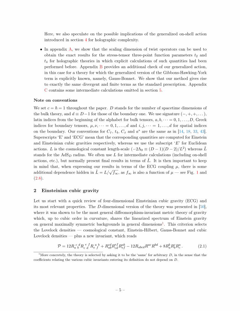
Figure 1. Real roots of (2.4) for different values of µ. The lower red dashed line corresponds to f∞ < 0,whereas the upper one corresponds to unstable vacua; the blue dashed line (µ < 0) corresponds tostable vacua which do not allow for black hole solutions — see discussion under (3.8); the purple dotcorresponds to the critical case, µ = 4/27; finally, the small green region corresponds to the set ofparameters allowed by the positive-energy constraint |t4| ≤ 4 in (7.29).

graviton becomes a ghost, and the corresponding vacuum is unstable. This imposes µ < 0

or f2∞ < 1/(3µ) for positive values of µ. The condition kills one of the two positive roots of

(2.4) available for 0 < µ < 4/27, which would then correspond to unstable vacua. Hence, weconclude that, whenever (2.5) is satisfied, there exists a single stable vacuum. No additionalvacua exist for µ < 0, whereas an additional unstable vacuum exists for 0 < µ < 4/27.Special comment deserves the f2

∞ = 1/(3µ) case, corresponding to µ = 4/27, and for whichGeff → +∞. This ‘critical’ limit of the theory was identified in [61], and gives rise to aconsiderable simplification of most calculations, as we further illustrate below.

We summarize these observations in Fig. 1, were we also include two additional constraintswhich we derive in sections 3 and 7.3, respectively. The first comes from imposing the existenceof black holes solutions, which restricts the allowed values to 0 ≤ µ ≤ 4/27. The secondfollows from the positivity of energy fluxes at null infinity which, as we can see from thefigure, produces the very stringent constraint, −0.00322 ≤ µ ≤ 0.00312.

Throughout the paper, we will assume µ to lie in the range 0 ≤ µ ≤ 4/27. From the twopositive roots of (2.4) in that range, we will be implicitly choosing the one corresponding to astable vacuum, which is also the one connecting to the Einstein gravity one for µ→ 0. Whilethe positive-energy condition further limits this range, we find it convenient to also considervalues close to µ = 4/27, for which many exact results can be obtained. Let us finally pointout that the solution of (2.4) corresponding to the relevant root (blue in Fig. 1) can be writtenexplicitly as

f∞ =2√3µ

sin

[1

3arcsin

(√27µ

4

)]. (2.8)

– 8 –

3 AdS4 black holes

ECG admits static asymptotically AdS4 black holes of the form

ds2 = −N2Vk(r)dt2 +

dr2

Vk(r)+r2

L2dΣ2

k , where dΣ2k =

L2dΩ2

2 , for k = +1 ,

d~x22 , for k = 0 ,

L2dΞ2 , for k = −1 ,

(3.1)

corresponding to spherical, planar and hyperbolic horizons, respectively, and where Vk(r) isdetermined from the second-order differential equation

1− L2(Vk − k)

r2− 3L6µ

4r3

[V ′3k3

+kV ′2kr−

2Vk(Vk − k)V ′kr2

−VkV

′′k (rV ′k − 2(Vk − k))

r

]=ω3

r3,

(3.2)where ω3 is an integration constant related to the ADM energy [65, 66] of the solution — see(6.5). Also, N2 is a constant that we fix in different ways depending on the horizon geometry,e.g., [25, 40, 43]. In particular, we will choose N2 = 1 for spherical horizons, N2 = 1/f∞ forplanar horizons, which sets the speed of light in the dual theory to one, and N2 = L2/(f∞R

2)

for hyperbolic horizons, so that the boundary metric is conformally equivalent to that ofR×H2, where R is the curvature scale of the hyperbolic slices.

The fact that ECG admits static solutions of the form (3.1), characterized by a singlefunction Vk(r), such that the full nonlinear equations4 of the theory reduce to a single third-order differential equation, which can in turn be integrated once to yield (3.2), is a highlynon-trivial property of ECG [51, 52]. Such property is shared by the higher-dimensionalLovelock [67–71], QTG [40, 41, 57, 59] (for these, the equation for Vk(r) is algebraic instead)and Generalized Quasi-topological [53] gravities, as well as by other higher-curvature theoriesof the same class, recently discovered and characterized [55, 56]. As mentioned before, thisproperty is related to the absence of extra modes in the linearized spectrum of the theory,and can be shown to lead to non-hairy black holes whose thermodynamic properties can becomputed analytically on general grounds [54].

In (3.1), it is customary to make the redefinition

Vk(r) = k +r2

L2f(r) , (3.3)

specially when dealing with the planar and hyperbolic cases. In terms of f(r), (3.2) reads

1− f + µ

[f3 +

3

2r2ff ′2 − r3

4f ′(f ′2 − 3ff ′′) +

3

4kL2f ′(rf ′′ + 3f ′)

]=ω3

r3. (3.4)

Observe that this reduces to (2.4) for constant f(r) and ω3 = 0. In particular, asymptotically,we require limr→+∞ f(r) = f∞, which then makes (3.1) become the metric of pure AdS4 withradius L given by (2.3), and a different boundary geometry for each value of k [72].

4These can be found explicitly e.g., in [51].

– 9 –

3.1 Asymptotic expansion

For general values of µ, finding analytic black hole solutions of (3.4) looks extremely chal-lenging (if not impossible). Let us then start by exploring the asymptotic and near horizonexpansions, from which we can gain a lot of relevant information (and, in fact, argue thatnon-hairy black hole solutions do really exist for general values of µ).

The first terms in the asymptotic expansion of f(r) read

f1/r(r) = f∞ −ω3

(1− 3µf2∞)r3

− 21µf∞ω6

2(1− 3µf2∞)3r6

+O(r−8) . (3.5)

Note that (3.4) is a second-order differential equation, which therefore possesses a two-parameter family of solutions. In order to capture the asymptotic behavior of the mostgeneral one, we write f(r) = f1/r(r) +h(r) and then expand (3.4) linearly in h. Keeping onlyleading terms in 1/r, we get the following equation for h5:

h′′(r)− 4(1− 3µf2∞)2

9f∞µω3rh(r) = 0 . (3.6)

Leaving aside the limiting cases, corresponding to µ = 0 and µ = 4/27, we see that thereare two possibilities, depending on the sign of µ · ω3. If µ · ω3 > 0, (3.6) has the followingapproximate solutions as r → +∞6:

h(r) ∼ A exp

[4|1− 3µf2

∞|9√f∞µ · ω3

r3/2

]+B exp

[−4|1− 3µf2

∞|9√f∞µ · ω3

r3/2

]. (3.7)

In order to obtain an asymptotically AdS4 solution, we need to kill the growing mode, whichforces us to set A = 0. Therefore, this boundary condition fixes one of the integration constantsrequired by (3.4). Now, even though the remaining exponentially decaying term is extremelysubleading, in general we will have B 6= 0. In fact, this constant ends up being fixed by thehorizon-regularity condition. In particular, this implies that the solutions show a stronglynonperturbative character, as ∼ e−1/

õ terms generically appear. Indeed, it is possible to

show that a series expansion of the full solution in powers of µ is always divergent.The second possibility corresponds to µ · ω3 < 0. An approximate solution of (3.6) for

large r is then given by

h(r) ∼ A

rcos

[4|1− 3µf2

∞|9√f∞|µ · ω3|

r3/2

]+B

rsin

[4|1− 3µf2

∞|9√f∞|µ · ω3|

r3/2

]. (3.8)

5For instance, we assume that the term h′L2r−4 is negligible compared to h′′r−1 when r → +∞.6The exact solution of (3.6) is given by the Airy functions,

h(r) = AAiryAi

[(4(1− 3µf2

∞)2

9f∞µω3

)1/3

r

]+BAiryBi

[(4(1− 3µf2

∞)2

9f∞µω3

)1/3

r

],

but we only need the asymptotic behavior for the discussion.

– 10 –

This solution is sick. Although h(r) → 0 as r → +∞, the derivatives of h diverge wildly inthis limit, which would force us to set A = B = 0 in order to get an asymptotically AdS4

solution. However, this leaves us with no additional free parameters, and regularity at the(would-be) horizon cannot be imposed. Therefore, no regular black hole solution exists forµ · ω3 < 0: the solution is always sick, either at the horizon or at infinity.

As shown later in (6.5), ω3 is proportional to the total energy E (or mass) of the blackhole, which leads us to impose µ ≥ 0. Hence, interestingly, the range of values of µ whichallows for positive-energy solutions, forbids the negative-energy ones, which simply do notexist for µ ≥ 0.

3.2 Near-horizon expansion

Let us now consider the near-horizon behavior. For that, we assume that there is a value rH ofthe radial coordinate for which the function Vk vanishes and is analytic. Analyticity ensuresthat the solution can be maximally extended beyond the horizon using Kruskal-Szekeres-likecoordinates.

The derivative of Vk at the horizon is related to the temperature through: V ′k(rH) =

4πT/N so, in terms of f , the near-horizon expansion can be written as

k +r2

L2f(r) =

4πT

N(r − rH) +

∞∑n=2

an(r − rH)n , (3.9)

where the relation between f ′(r) and the temperature reads in turn

T =N

4π

[rH

2

L2f ′(rH)− 2k

rH

]. (3.10)

Note also that f(rH) = −kL2/rH2. Now, if we plug (3.9) into (3.4) and we expand it in powers

of (r − rH), we are led to the equation

0 = 1 +kL2

rH2− ω3

rH3− 4L6π2T 2µ

N2rH3

(3k

rH+

4πT

N

)+ (3.11)[

−2kL2

rH2+

3ω3

rH3− 4L2πT

NrH+

24L6π2T 2µ

N2rH3

(k

rH+

2πT

N

)](r − rH) +O

((r − rH)2

). (3.12)

Since every coefficient must vanish independently, we get an infinite number of equationsrelating the parameters in the near-horizon expansion (3.9). From the first two equations,we can obtain TECG and ωECG as functions of rH, the result being (in order to minimize theclutter, we often omit the ‘ECG’ superscripts throughout the text)

TECG =N

2πrH

(k +

3rH2

L2

)[1 +

√1 +

3kL4µ

rH4

(k + 3

rH2

L2

)]−1

, (3.13)

(ωECG)3

= kL2rH + rH3 − µL6

4

[3k

rH

(4πTECG

N

)2

+

(4πTECG

N

)3]. (3.14)

– 11 –

These reduce to the usual Einstein gravity results for µ = 0, namely

TE =N

4πrH

(k +

3rH2

L2

), (ωE)

3= rH

3 + krHL2 . (3.15)

The rest of equations, which we do not show here, fix all coefficients an>2 in terms of a2.Hence, for a fixed rH, the series (3.9) contains a single free parameter, which is nothing butthe value of f ′′ at the horizon. This must be carefully chosen so that the solution has theappropriate asymptotic behavior, i.e., so that A = 0 in (3.7).

3.3 Full solutions

Equation (3.4) can be solved analytically in two cases, namely: for Einstein gravity, µ = 0,and in the critical limit, µ = 4/27 [61]. For those, one finds7

f(r) =

1− rH

3+kL2rHr3

if µ = 0 ,32 −

3rH2+2kL2

2r2if µ = 4/27 .

(3.18)

For intermediate values of µ, the solutions can be constructed numerically. In order to doso, we solve (3.4) setting the initial condition at the horizon, and then applying the shootingmethod to obtain the value of a2 for which f(r) → f∞. The differential equation (3.4) isvery stiff when r is large but, by choosing a2 accurately, it is always possible to extend thenumerical solution well into the region in which the asymptotic expression (3.5) applies. Inall cases, there is a unique value of a2 for which this happens. Hence, for each value of µ andeach horizon geometry, there exists a unique regular black fully characterized by rH (or, morephysically, by ωECG).

In Fig. 2 we show a couple of these numerical solutions for rH = 1.5L. As we can see,the corresponding curves lie between the analytic limiting solutions in (3.18). Far from thehorizon, the functions f(r) tend to the constant values f∞ which, as explained above, aredifferent for each value of µ — see Fig. 1. Besides the exterior solutions, we also show plotsof the black hole interior profiles8, which present the curious feature of having regular metrics

7A curious property of the critical-theory solutions is that they look identical to three-dimensional BTZblack holes [73], with an additional ‘angular’ direction:

ds2ECG, crit = −3(r2 − rH2)

2L2dt2 − 2L2dr2

3(r2 − rH2)+r2

L2dΣ2

(k) , (3.16)

ds2BTZ = − (r2 − rH2)

L2dt2 − L2dr2

(r2 − rH2)+ r2dφ2 . (3.17)

We point out that an analogous behavior has been observed to occur for critical Gauss-Bonnet gravity (λGB =

1/4), see e.g., [37] as well as for Einstein gravity coupled to an axionic field in a particular limit [74]. Theconnection of this phenomenon to other instaces of background-symemtry enhancement — e.g., [75] — deservesfurther attention.

8For the sake of visual clarity, we present the interior and exterior solutions in different figures, plottingVk(r) for the former, and f(r) for the latter.

– 12 –

-

μ=

μ=

μ=/

-

-

-

-

-

/

+/()

-

μ=

μ=

μ=/

-

/

()

-

μ=

μ=

μ=/

-

-

-

-

-

/

/()

-

μ=

μ=

μ=/

/()

-

μ=

μ=

μ=/

-

-

-

-

-

/

-+/()

-

μ=

μ=

μ=/

/

()

Figure 2. Black hole solutions for several values of µ (we take rH = 3L/2), including the Einsteingravity (µ = 0) and critical (µ = 4/27) cases. From top to bottom k = 1, 0,−1. For the sake ofclarity, we have made separate plots for the interior and exterior solutions. In the left column, we plotVk(r) = k + r2/L2f(r) for the black-hole interior range. In the right column we plot f(r) instead forthe exterior solutions.

at r = 0. However, as observed in [52] for the asymptotically flat case, curvature invariantsstill diverge. For example, in the critical case, one finds

RabcdRabcd =

4k2L4 + 54r4 − 6rH2r2 + rH

4 − 4kL2(3r2 − rH2)

L4r4∼ O

(r−4), (3.19)

which is two powers of r softer than in the usual Schwarzschild case. Such behavior is commonto all solutions with µ 6= 0. This singularity-softening phenomenon appears to be generic forhigher-curvature generalizations of Einstein gravity black holes. For example, for the Gauss-Bonnet black hole [70], one finds [76] RabcdRabcd ∼ O(r−(D−1)), which is in turn (D − 1)

powers of r softer than the Kretschmann invariant of the D-dimensional Schwarzschild blackhole.

– 13 –

4 Generalized action for higher-order gravities

When performing holographic calculations with higher-curvature bulk duals, one is faced withthe challenge of identifying appropriate boundary terms which render the action differentiable,as well as counterterms which, along with those, give rise to finite and well-defined on-shellactions, when evaluated on stationary points of the functional. In this section, we propose anovel prescription for computing the on-shell action of arbitrary asymptotically AdS solutionsof any D-dimensional higher-order gravity whose linearized spectrum on a maximally sym-metric background matches that of Einstein gravity9. The procedure represents an importantsimplification with respect to previous methods, as it only makes use of the usual Gibbons-Hawking-York boundary term and the counterterms of Einstein gravity. As we argue here —and illustrate throughout the rest of the paper and in appendix B with various non-trivialchecks of the proposal — such contributions can be also used to produce the correct on-shellactions for this class of higher-order theories. Interestingly, for those, the only modificationwith respect to the Einstein gravity case is that such contributions appear weighted by theLagrangian of the corresponding theory evaluated on the AdS background, i.e., L|AdS. Thisquantity has been argued to be proportional to the charge a∗ appearing in the universal con-tribution to the entanglement entropy of the dual theory across a Sd−2, and our prescriptioncan be used to actually prove such a connection explicitly for this class of theories, as we showbelow.

Let us start considering a general higher-curvature theory of the form

I =

∫MdDx

√|g|L(gef , Rabcd) , (4.1)

where the Lagrangian density L(gef , Rabcd) is assumed to be constructed from arbitrary con-tractions of the Riemann and metric tensors. The variation of the action with respect to themetric yields

δI =

∫MdDx

√|g|Eabδgab + ε

∫∂M

dD−1x√|h|naδva . (4.2)

In this expression we defined

Eab ≡ Pa cdeRbcde −1

2gabL − 2∇c∇dPacdb , (4.3)

the equations of motion reading Eab = 0, and

δva = 2gdcP abed ∇eδgbc , where P abcd ≡

[∂L

∂Rabcd

]gef

. (4.4)

In addition, na is the unit normal to ∂M, normalized as nana ≡ ε = ±1, and hab =

gab − εnanb is the induced metric. In order to have a well-posed variational problem, the9This property defines the ‘Einstein-like’ class in the classification of [64], and includes, in particular:

Lovelock, QTG, ECG in general D and, more generally, all theories of the Generalized QTG type. Additionalexamples of theories of this type can be found e.g., in [77–80].

– 14 –

action must be differentiable, in the sense that δI ∝ δgab, so that δI = 0 whenever thefield equations — and the boundary conditions — are satisfied. This is not the case of(4.2), due to the presence of the boundary contribution. In the case of Einstein grav-ity, LE =

[R+ (D − 1)(D − 2)/L2

]/(16πG), this problem is solved by the addition of the

Gibbons-Hawking-York term [81, 82],

IGHY =ε

8πG

∫∂M

dD−1x√|h|K , (4.5)

where K = Kabgab is the trace of the second fundamental form of the boundary, Kab =

h ca ∇cnb. When this term is included, the variation of the action, when we keep gab fixed at

the boundary, reads

δ(IE + IGHY)∣∣∣δgab|∂M=0

=1

16πG

∫Md4x√|g|[Rab −

1

2gabLEH

]δgab , (4.6)

and so the action is stationary whenever the metric satisfies Einstein’s field equations.For higher-order gravities, the situation is much more involved in general. One of the

main issues arises from the fact that these theories generally posses fourth-order equations ofmotion. This implies that the boundary-value problem is not fully specified by the inducedmetric on ∂M, and one needs to impose additional boundary conditions on derivatives of themetric. Furthermore, even if we know which components of the metric and its derivatives tofix, determining what boundary term needs to be added to yield a differentiable action for suchvariations is a far from trivial task. Some notable examples for which differentiable actionshave been constructed are: quadratic gravities (perturbatively in the couplings) [83], Lovelockgravities [84, 85], which are the most general theories with second-order covariantly-conservedfield equations [29, 30] (and for which one only needs to fix gab at the boundary), f(R) [86–88]and, more generally, f(Lovelock) gravities [78]. In these cases, it is also necessary to fix thevalue of some of the densities on the boundary — e.g., δR

∣∣∂M = 0 for f(R) — which is

related to the fact that these theories propagate additional scalar modes. With the goal ofproviding a canonical formulation for arbitrary f(Riemann) gravities, an interesting proposalfor constructing satisfactory boundary terms for such general class of theories was presentedin [89] — see also [90]. Unfortunately, the procedure involves the introduction of auxiliaryfields and it is quite implicit in general, which seems to limit its practical applicability in theholographic framework.

The problem can be simplified if we specify the boundary structure in advance, e.g., byrestricting the analysis to spacetimes which are maximally symmetric asymptotically. Letus, in particular, assume that the space is asymptotically AdSD, so that the Riemann tensorbehaves as Rabcd → −L−2(gacgbd − gadgbc) asymptotically. Then, on general grounds, thetensor P ab

cd appearing in the boundary term in (4.2) takes the simple form

P abcd → C(L2)δ a

[c δbd] + subleading , (4.7)

– 15 –

where C(L2) is a constant which depends on the background curvature, and is in general givenby10 [64]

C(L2) = − L2

2(D − 1)L|AdS , (4.9)

where L|AdS is the Lagrangian of the corresponding theory evaluated on the AdSD backgroundwith curvature scale L.

For Einstein gravity, we simply have CE = 1/(16πG) and, in fact, there are no subleadingterms in (4.7) for any spacetime — simply because P ab

cd only involves products of deltas inthat case. Now, asymptotically AdSD solutions of higher-order gravities will in general producesubleading contributions in (4.7) as we move away from the asymptotic region. However, theleading term can still be canceled out by adding a generalized GHY term of the form

IGGHY = 2C(L2)ε

∫∂M

dD−1x√|h|K . (4.10)

The question is, of course, whether or not the subleading terms for a given theory will giveadditional non-vanishing contributions asymptotically, forcing us to add extra terms. Weexpect this to be the case in general. In addition, one generally needs to specify extra boundaryconditions, which is related to the metric propagating additional degrees of freedom. However,as we have mentioned, some theories — see footnote 9 — do not propagate additional modeson general maximally symmetric backgrounds. For those, the asymptotic dynamics is thesame as for Einstein gravity, so it is reasonable to expect the only data that we need to fix on∂M to be gab, and also that (4.10) will be enough to make the action stationary for solutionsof the field equations.

In order to obtain finite on-shell actions, one also needs to include counterterms, whichonly depend on the boundary induced metric. For asymptotically AdSD spacetimes, there isa generic way of finding them [72]. Let us focus on Euclidean signature. In that case, wealways have ε = +1, and an additional global (−) with respect to Lorentzian signature arises,e.g., [14], so we have

IE = −∫MdDx√gL(gef , Rabcd)− 2C(L2)

∫∂M

dD−1x√|h|K + IGCT , (4.11)

where we seek to construct the generalized counterterms, IGCT. In order to identify all possibledivergences, one possibility consists in evaluating the action on pure AdSD spaces with differentboundary geometries [91]. Observe however that, whenever we evaluate the bulk term on pureAdSD, this will produce an overall constant L|AdS, which is precisely proportional to C(L2).This already appears in front of the boundary term, and the result is that the combination

10As shown in [64], this quantity can be equivalently written as

C(L2) =L4

D(D − 1)

dL|AdS

dL2, (4.8)

the relation between both expressions being nothing but the embedding equation of AdSD in the correspondingtheory — e.g., (2.4) for ECG.

– 16 –

of the bulk and boundary contributions reduce to those of Einstein gravity, up to a commonoverall C(L2). Hence, the divergences are exactly the same as for Einstein gravity, and wecan use the same counterterms. For example, up to D = 5 we find [72, 91]

IGCT = −2C(L2)

∫∂M

dD−1x√h

[− D − 2

L− LΘ[D − 4]

2(D − 3)R+ . . .

], (4.12)

where Θ[x] = 1 if x ≥ 0, and zero otherwise, and the dots refer to additional countertermsarising for D ≥ 6. Combining (4.12) with (4.11), we obtain the final form of the action.

Below, we show that (4.11) successfully yields the right answers for ECG in various highlynon-trivial situations in which the corresponding on-shell actions can be deduced from alter-native considerations — e.g., it correctly computes the free energy of black holes, in agreementwith the result obtained using Wald’s entropy, as well as the holographic stress tensor two-point charge, CT , which can be alternatively deduced from the effective Newton constant.Besides, in appendix B we consider arbitrary radial perturbations of AdS5 in Gauss-Bonnetgravity, and show that (4.11) produces exactly the same finite and divergent contributionsas those obtained using the standard Gauss-Bonnet boundary term and counterterms, e.g.,[72, 84, 85, 92–95].

4.1 a∗ and generalized action

Let us momentarily switch to d ≡ D − 1 notation. As we have seen, both the boundaryterm and the counterterms appearing in (4.11) have the property of being identical to thoseof Einstein gravity up to an overall constant C(L2) proportional to the Lagrangian of thecorresponding theory evaluated on the AdS background (4.9). Now, an interesting quantitythat one would like to compute holographically is the charge a∗ appearing in the universalcontribution to the entanglement entropy (EE) across a radius-R spherical region Sd−2 which,for a general CFTd, is given by [14, 15, 96]

SEEuniv. =

(−)

d−22 4a∗ log(R/δ) for even d ,

(−)d−12 2πa∗ for odd d .

(4.13)

a∗ coincides with the a-type trace-anomaly charge in even dimensional theories. In odd di-mensions, a∗ is proportional to the free energy, F = − logZ, of the corresponding theoryevaluated on Sd [96], namely

FSd = (−)d+12 2πa∗ , for odd d . (4.14)

For even-dimensional holographic theories dual to any higher-order gravity of the form (4.1)in the bulk, a∗ is given by [97, 98]

a∗ = −πd/2Ld+1

dΓ(d/2)L|AdS , (4.15)

– 17 –

i.e., it is precisely proportional to the charge C(L2) defined in (4.9), namely

C(L2) =a∗

Ω(d−1)Ld−1, (4.16)

where Ω(d−1) ≡ 2πd/2/Γ(d/2) is the area of the unit sphere Sd−1. For odd-dimensional theories,it was argued in [14, 15] that (4.15) also yields the right a∗ for general cubic theories. Wecan readily extend this result to all theories for which (4.11) and (4.12) hold. From (4.14), itfollows that (−)

d+12 2πa∗ can be obtained from the on-shell action of pure Euclidean AdS(d+1)

with boundary geometry Sd. Since C(L2) appears as an overall factor in (4.11) when evaluatedin pure AdS, it follows that FSd matches the Einstein gravity result up to an overall factor16πG · C(L2). Then, using the result for the free energy in Einstein gravity,

FESd = (−)

d+12πd/2Ld−1

4Γ(d/2)G, (4.17)

it follows immediately that for any theory of the form (4.1), for which our generalized on-shellaction can be used,

FSd = 16πG · C(L2)FESd = (−)

d−12

2πd/2+1Ld+1

dΓ(d/2)L|AdS , (4.18)

which takes the expected general form (4.14), with a∗ precisely given by (4.15). Hence, wehave obtained the expected form of the charge a∗ from an explicit holographic calculation ofthe free energy on Sd using our generalized action. The consistency between (4.11) and (4.15)provides support for both expressions.

Reversing the logic, we can rewrite our generalized action in terms of a∗, which is waymore charismatic than C(L2). The result reads

IE = −∫MdDx√gL(gef , Rabcd)−

2a∗

Ω(d−1)Ld−1

∫∂M

dD−1x√|h|[K − d− 1

L+ · · ·

], (4.19)

where we have omitted most of the counterterms in (4.12). The explicit appearance of a∗ inthe boundary terms is rather suggestive, and somewhat striking. In section 9 we comment onthe possible implications of (4.19) for holographic complexity.

4.2 Generalized action for Quasi-topological gravity

The QTG density in five bulk dimensions is given by [40, 41]

Z5 = R c da b R

e fc d R

a be f +

1

56

(− 72RabcdR

abceR

de + 21RabcdRabcdR+ 120RabcdR

acRbd

+ 144RbaRcbR

ac − 132RabR

abR+ 15R3).

(4.20)

Just like ECG in D = 4, the linearized equations of this theory on constant-curvature back-grounds are Einstein-like [40]. Hence, the method developed in the previous subsection should

– 18 –

be valid for computing Euclidean on-shell actions of AdS5 solutions of the theory. In this case,the full generalized action (4.19) is given by

IQTGE = − 1

16πG

∫Md5x√g

[12

L2+R+

L2λ

2X4 +

7µL4

4Z5

]− 1− 6λf∞ + 9µf2

∞8πG

∫∂M

d4x√h

[K − 3

√f∞L− L

4√f∞R

],

(4.21)

where we also included the Gauss-Bonnet density X4 = R2 − 4RabRab + RabcdR

abcd. In thiscase, the charge a∗ reads [43]

a∗QTG =(1− 6λf∞ + 9µf2

∞) πL3

8G, (4.22)

while f∞ is determined by the equation [40]

1− f∞ + λf2∞ + µf3

∞ = 0 . (4.23)

A generalized boundary term for QTG was proposed in [99]. It would be interesting to checkwhether (4.21) provides the same results as those obtained using such term. As we mentionedabove, in appendix B we perform an explicit check of that kind for Gauss-Bonnet gravity.

4.3 Generalized action for Einsteinian cubic gravity

Let us now return to ECG. In that case, the full generalized Euclidean action (4.19) becomes

IECGE =− 1

16πG

∫d4x√|g|[

6

L2+R− µL4

8P]

− 1 + 3µf2∞

8πG

∫∂M

d3x√h

[K − 2

√f∞L− L

2√f∞R],

(4.24)

where recall that f∞ can be obtained as a function of µ from (2.4). Observe also that thecharge a∗ reads in this case

a∗ECG = (1 + 3µf2∞)

L2

4G. (4.25)

We use (4.24) in several occasions in the remainder of the paper, finding exact agreement withthe expected results in all cases for which alternative methods can be used.

5 Stress tensor two-point function charge CT

In order to characterize the holographic dual of ECG, we must translate the two availabledimensionless parameters in (2.2), namely: L2/G and µ, into universal defining quantities ofthe boundary theory. Since we are only considering the gravitational sector of the bulk theory,the most relevant ‘charges’ to be identified in the CFT are those characterizing the boundarystress tensor. Conformal symmetry highly constrains the structure of stress-tensor two- and

– 19 –

three-point functions [100]. We will deal with the three-point function charges in section 7.3.Let us start here with the stress-tensor correlator which, for an arbitrary CFT3, is given by[100]

〈Tµν(x)Tρσ(x′)〉 =CT

|x− x′|6Iµν,ρσ(x− x′) , (5.1)

where

Iµν,ρσ(x) ≡ 1

2(Iµρ(x)Iνσ(x) + Iµσ(x)Iνρ(x))− 1

4δµνδρσ , and Iµν(x) ≡ δµν−2

xµxνx2

, (5.2)

are fixed tensorial structures. This correlator is then fully characterized by a single theory-dependent parameter, customarily denoted CT . This quantity, which in even dimensions isproportional to the trace anomaly charge c, also plays a relevant role in three-dimensionalCFTs — see e.g., [101–103] for recent studies. As opposed to the d = 2 case [104], CT

is not monotonous under general RG flows in three dimensional CFTs [105]. However, ituniversally shows up in various contexts, including relevant quantities in entanglement andRényi entropies [16, 17, 25, 26, 106]; quantum critical transport — see e.g., [107, 108] andreferences therein; or partition functions on deformed curved manifolds [109–111].

In AdS/CFT, the dual of Tµν(x) is the normalizable mode of the metric [2, 3]. Hence,evaluating (5.1) entails determining the two-point boundary correlator of gravitons in thecorresponding AdS vacuum. For Einstein gravity in d = 3, the result [33, 112] reads

CET =

3

π3

L2

G. (5.3)

Naturally, the introduction of higher curvature terms in the bulk modifies this result, e.g.,[18, 33, 43]. In general, higher order gravities give rise to equations of motion involving morethan two derivatives of the metric. In those cases, the metric generically contains additionaldegrees of freedom besides the usual massless graviton. From the holographic perspective,this means that the metric couples to additional operators which are typically nonunitary11.This is not always the case, however. In fact, there exist families of higher order gravitieswhose linearized equations around maximally symmetric backgrounds are identical to thoseof Einstein gravity, up to a normalization of the Newton constant — see footnote 9 and e.g.,[64] for details. For those, the only mode is the usual spin-2 graviton, the metric only couplesto the stress tensor, and CT can be straightforwardly extracted from the effective Newtonconstant. This generically reads Geff = G/α, where α is a constant which depends on the newcouplings. The appearance of α can be alternatively understood as changing the normalizationof the graviton kinetic term which, holographically, gets translated into a modification of thestress-tensor correlator charge, which then becomes α · CE

T .For ECG, using (2.7), we find then

CECGT = (1− 3µf2

∞)3

π3

L2

G. (5.4)

11See e.g., [14, 18] for more detailed discussions of this issue.

– 20 –

Observe that unitarity imposes CT to be positive, which translates into 1−3µf2∞ > 0. This is

of course equivalent to asking the effective bulk gravitational constant to be positive. It canbe seen that this constraint is automatically satisfied whenever (2.5) holds.

While we have been able to compute CT for ECG using GECGeff , it is instructive to obtain it

from an explicit holographic calculation. This will also serve as a highly-nontrivial consistencycheck for the new on-shell action method introduced in the previous section.

Let us then consider a metric perturbation: gab = gab + hab, on the Euclidean AdS4

vacuum

ds2 =r2

L2

[dτ2 + dx2 + dy2

]+

L2

r2f∞dr2 . (5.5)

Since all components of the two-point function will be determined by CT , computing oneof them will be enough. It is then sufficient to consider a perturbation of the form hxy =r2

L2φ(r, τ). Plugging this into the Euclidean version of (2.2) and expanding up to quadraticorder in φ, we find

IECGE Bulk =

(1− 3µf2∞)

32πG

∫d3xdr

[1√f∞

(∂τφ)2 +√f∞

r4

L4(∂rφ)2

]− 1

16πG

∫d3xΓr

∣∣∣r=r∞

,

(5.6)where Γr is a boundary term which appears after integration by parts — see (C.2). Recall alsothat, in this coordinates, the boundary corresponds to limr→∞ r ≡ L2/δ, where we introducethe UV cutoff δ 1. The equation of motion for φ follows from (5.6), and reads

∂

∂r

(r4

L4

∂φ

∂r

)+

1

f∞

∂2φ

∂τ2= 0 . (5.7)

In order to solve it, we Fourier-transform the dependence on the coordinate τ ,

φ(r, τ) =1

2π

∫dpφ0(p)eipτHp(r) . (5.8)

Hp satisfies the equationd

dr

(r4

L4

dHp

dr

)− p2

f∞Hp = 0 , (5.9)

whose general solution reads

Hp(r) = c1e− L2|p|√

f∞r

(1 +

L2|p|√f∞r

)+ c2e

L2|p|√f∞r

(1− L2|p|√

f∞r

). (5.10)

In order to get a regular solution, we set c2 = 0, and we also fix c1 = 1 so that Hp(r →L2/δ) = 1. With this solution, we evaluate the Lagrangian, which can be expressed as a totalderivative. Further integrating over the r coordinate and substituting the solution in Fourierspace, we get

IECGE Bulk =

√f∞VR2

64π2GECGeff

∫dpdqφ0(p)φ0(q)δ(p+ q)

L4

δ4Hp∂rHp

∣∣∣r=L2/δ

− 1

16πG

∫d3xΓr

∣∣∣r=L2/δ

,

(5.11)

– 21 –

where VR2 =∫dxdy, and where we used

∫dτei(p+τ) = 2πδ(p+ q).

Let us now turn to the boundary contributions in the generalized action (4.24). As weexplain in appendix C, when these terms are added to (5.11), most divergences in Γr

∣∣∣r=L2/δ

disappear, and we are left with the following result for the full action:

IECGE = IECG

E Bulk + IECGEGGHY+GCT (5.12)

=VR2

64π2GECGeff

√f∞

∫dpdqφ0(p)φ0(q)δ(p+ q)

[f∞

L4

δ4Hp∂rHp

∣∣∣r=L2/δ

− L2p2

δH2p

].

Observe that, even though 1/GECGeff and a∗ECG have a different dependence on µ — see (2.7)

and (4.25) respectively — and that it is a∗ECG the one appearing as an overall constant in thegeneralized GHY term and the counterterms (4.24), everything conspires to produce a singlefinite contribution which is instead proportional to 1/GECG

eff , as it must.If we take the limit δ → 0 explicitly in (5.12), we get the simple result

IECGE [φ0] = − VR2L2

64π2Geff

∫dpdqφ0(p)φ0(q)δ(p+ q)|p|3 . (5.13)

Using the holographic dictionary [3], we can compute one of the components of the boundarystress tensor two-point function in momentum space as

〈Txy(0, 0, p)Txy(0, 0, q)〉 = −(2π)2 δ2IECGE [φ0]

δφ0(−p)δφ0(−q)=L2VR2

8Geffδ(p+ q)|p|3 . (5.14)

Now, from the CFT side, this is given by

〈Txy(0, 0, p)Txy(0, 0, q)〉 =

∫d3x

∫d3x′e−ipτe−iqτ

′〈Txy(x)Txy(x′)〉 , (5.15)

where

〈Txy(x)Txy(x′)〉 =

CT

2|x− x′|6

[−1 + 2

(τ − τ ′)2

|x− x′|2+ 8

(x− x′)2(y − y′)2

|x− x′|4

]. (5.16)

The integration in (5.15) can be performed without further complications and we obtain theresult

〈Txy(0, 0, p)Txy(0, 0, q)〉 =π3CTVR2

24δ(p+ q)|p|3 . (5.17)

Comparing this expression with (5.14), we obtain the result for CT , which agrees with the onein (5.4), as it should. The fact that our generalized action (4.24) succeeds in providing theright answer for this quantity, including various non-trivial cancellations between IECG

E Bulk andIECGEGGHY+GCT — see appendix C — provides strong evidence for the validity of the methoddeveloped in section 4.

Note finally that, as explained at the beginning of this section, CT provides informationabout many different physical quantities appearing in numerous contexts. Hence, by the sameprice we computed (5.4), we gain access to all such quantities for the CFT3 dual to ECG.

– 22 –

6 Thermodynamics

In this section we study the thermodynamic properties of the ECG black holes constructed insection 3. First, we compute the Wald entropy, ADM energy and free energy of the solutions,and compare the result with the one obtained from an explicit on-shell action calculation,which serves as a further check of the method proposed in section 4. Then, focusing on theflat boundary case, k = 0, we identify the quantity CS which relates the thermal entropydensity to the temperature, and show that, in contradistinction to Einstein gravity, it definesan independent charge with respect to CT . In subsections 6.3 and 6.4, we study the phasespace of holographic ECG on S1

β×T2 and S1β×S2, respectively. In the first case, we show that

the standard phase transition between the ECG AdS soliton and black brane keeps occurringat the same temperature as for Einstein gravity. In the second, we show that depending on thevalue of µ, one, two or three black hole solutions can coexist at the same temperature. Thedominating phases are still thermal AdS at small temperatures and large black holes at largetemperatures, but the Hawking-Page-transition temperature becomes arbitrarily large as weapproach the critical limit µ = 4/27. Besides, small black holes become thermodynamicallystable for µ 6= 0, although their contribution to the partition function is always subleadingwith respect to thermal AdS.

6.1 Entropy, energy and free energy

Let us start by computing the Wald entropy of the solutions which, for any covariant theoryof gravity is given by [113, 114]

S = −2π

∫H

dd−1x√h

∂L∂Rab cd

εabεcd , (6.1)

where εab is the binormal to the horizon. Now, for metrics of the form (3.1), the integrationcan be performed straightforwardly, yielding

S = −2πrH2

L2VΣ

∂LECG

∂Rab cdεabεcd

∣∣∣∣r=rH

, (6.2)

where VΣ is the regularized volume of S2, R2 or H2 for k = 1, 0,−1 respectively. Explicitly,the final result for the ECG black holes reads

SECG =rH

2VΣ

4GL2

1−3µL4

(k + 3rH

2

L2

)[(k + 3rH

2

L2

)+ 2k

[1 +

√1 + 3kL4µ

rH4

(k + 3 rH

2

L2

)]]rH4

[1 +

√1 + 3kL4µ

rH4

(k + 3 rH

2

L2

)]2

.(6.3)

Again, this reduces to the Einstein gravity result

SE =rH

2VΣ

4GL2, (6.4)

– 23 –

when we set µ = 0. Once we have S(T ) (defined implicitly), we can use the first law,dE = TdS, to find the energy. The result is

EECG =(ωECG)

3VΣN

8πGL4. (6.5)

As expected, this coincides with the result one would obtain for the generalized ADM energyfrom the asymptotic expansion (3.5).

The entropy of the solutions can be alternatively computed from the free energy as S =

−∂F/∂T . Hence, we can perform an additional check of our generalized action (4.24), whichevaluated on the Euclidean version of the solutions — for which we identify tE ∼ tE + β —should yield the free energy as FECG = IECG

E /β. Plugging (3.1) in (4.24), we find that thebulk term is a total derivative that can be integrated straightforwardly, namely

IECGE Bulk =

βNVΣ

16πGL2

[H(rH)−H(L2/δ)

], (6.6)

where

H(r) ≡ r3

L2

[(2− 4f − rf ′)− µ

4

(2f + rf ′

)2 (4f − rf ′

)]. (6.7)

Using the asymptotic expansion (3.5), we get

H(L2/δ) =2L4

δ3(1− 2f∞ − 2µf3

∞) +(ωECG)

3

L2

(1 + 3µf2∞)

(1− 3µf2∞)

+O(δ) . (6.8)

We can also evaluate the boundary contributions in (4.24). For these, we use

d3x√h = Ndt ∧ dΣk

(√f∞L

3

δ3+

kL

2δ√f∞− (ωECG)

3

2√f∞L3(1− 3µf2

∞)

)+O(δ) ,

K =3√f∞L

+kδ2

2L3√f∞

+O(δ4) , R =2kδ2

L4.

(6.9)

Then, we find

IECGEGGHY+GCT = −βNVΣ(1 + 3µf2

∞)

8πGL4

[L6f∞δ3

− (ωECG)3

2(1− 3µf2∞)

]+O(δ) . (6.10)

Now, if we add up both contributions we obtain the finite result

IECGE =

βNVΣ

16πGL2H(rH) , (6.11)

where we made use of the AdS4 embedding equation (2.4). Hence, all boundary contributionscancel out and the on-shell action is reduced to the evaluation of the function H(r) at thehorizon. Using the near-horizon expansion (3.9), we can finally write the free energy as

FECG =NVΣ

8πGL2

[krH +

rH3

L2− 2πTrH

2

N+ µL4

(3k

rH

(2πT

N

)2

+

(2πT

N

)3)]

. (6.12)

– 24 –

Note that this can be also written fully in terms of rH using (3.13). When µ = 0, (6.12)reduces to the Einstein gravity result

FE =NVΣrH16πGL2

(k − rH

2

L2

). (6.13)

Using (6.12) and the thermodynamic identity S = −∂F/∂T , we can recompute the entropyof the solutions. The result precisely matches (6.3), computed using Wald’s formula, whichprovides another check for our generalized action.

6.2 Thermal entropy charge CS

When the boundary geometry is flat, k = 0, it is convenient to set N2 = 1/f∞, a choicewhich fixes the speed of light to one in the dual CFT [33]. In that case, the thermodynamicexpressions simplify considerably. In particular, we find

T =3rH

4πL2√f∞

, ω3 = rH3

(1− 27

4µ

), (6.14)

s =rH

2

4GL2

(1− 27

4µ

), ε =

rH3

8πGL4√f∞

(1− 27

4µ

), (6.15)

where we defined the entropy and energy densities s ≡ S/VR2 , ε ≡ E/VR2 . We can explicitlywrite these quantities in terms of the temperature, the result being

s =4π2L2f2

∞9G

(1− 27

4µ

)T 2 , ε =

8π2L2f2∞

27G

(1− 27

4µ

)T 3. (6.16)

From (6.16), it immediately follows that ECG black branes satisfy

ε =2

3Ts , (6.17)

as expected for a thermal plasma in a general three-dimensional CFT.The dependence on the temperature of the thermal entropy density is also fixed for any

CFT3 to take the forms = CST

2 , (6.18)

where CS is a theory-dependent quantity. From, (6.16), it follows that

CECGS =

(1− 27

4µ

)f2∞C

ES , where CE

S =4π2

9

L2

G, (6.19)

is the Einstein gravity result — see e.g., [33]. As we can see, in the holographic modeldefined by ECG, CS is no longer proportional to CT , and therefore defines an additional well-defined independent ‘charge’ which characterizes the theory12. For growing values of µ, CS

12Observe that CS can be rewritten as CECGS = f2

∞(1−3µf2∞/4)(1−3µf2

∞)2CES , which makes it more obvious

that this charge is not proportional to CECGT .

– 25 –

monotonously decreases with respect to the Einstein gravity value and, funnily, it vanishes forthe critical case13 , µ = 4/27.

The fact that CS vanishes for certain value of the gravitational coupling is quite unusual,and does not occur for QTG or Lovelock black holes (in the Einstein gravity branch) in anynumber of dimensions — see e.g., [33, 40, 43, 71, 115]. In fact, in those cases, the onlymodification in CS with respect to Einstein gravity is an overall f (d−1)

∞ factor, i.e., the resultreads CQTG/Lovelock

S = f(d−1)∞ CE

S , where CES is the Einstein gravity result written in terms

of L. In fact, in view of the results for those theories, one would have naively expectedall ‘(1 − 27/4µ)’ factors in (6.14)-(6.19) not to appear for ECG. This seems to be a simplemanifestation of the fact that the theories belonging to the Generalized QTG class (includingECG) for which f(r) is determined through a second-order differential equation possess ratherdifferent properties from those for which f(r) is determined from an algebraic equation — seebelow and [53–55, 60] for more evidence in this direction.

6.3 Toroidal boundary: black brane vs AdS4 soliton

In this subsection we study the phase space of thermal configurations when the spatial dimen-sions of the boundary CFT form a torus T2. The first obvious saddle corresponds to EuclideanAdS4 with toroidal boundary conditions, given by

ds2 =r2

L2

[dτ2 + dx2

1 + dx22

]+

L2

r2f∞dr2 , (6.20)

where the coordinates x1 and x2 are assumed to be periodic, x1,2 ∼ x1,2 + l1,2, where l1,2 is theperiod of each coordinate. Without loss of generality we assume l1 ≤ l2. As before, τ ∼ τ +β.The next candidate is the Euclidean black brane

ds2 =r2

L2

[f(r)

f∞dτ2 + dx2

1 + dx22

]+

L2

r2f(r)dr2 , (6.21)

for which the temperature is fixed in terms of the horizon radius through (6.14). Finally, itshould be evident that moving the f(r)/f∞ factor from gττ to g11 or g22 should also give riseto solutions of ECG, e.g.,

ds2 =r2

L2

[dτ2 +

f(r)

f∞dx2

1 + dx22

]+

L2

r2f(r)dr2 . (6.22)

These are the so called AdS4 ‘solitons’ [116, 117]. The crucial difference with respect to theblack brane is that, for these, regularity no longer imposes a relation between the temperatureand the horizon radius. Instead, it fixes the periodicity of x1 (or x2 if f(r)/f∞ appears in g22

instead) in terms of rH as

l1,2 =4πL2

√f∞

3rH. (6.23)

13This would seem to suggest that the black brane has a unique microstate in that case, but it is probablyjust another evidence of the problematic properties of the critical theory.

– 26 –

Of course, τ is still periodic with period β, but, as opposed to the black-brane case, thetemperature can be now arbitrary for a given value of rH.

Now, the Euclidean action vanishes for pure Euclidean AdS4, whereas for the black braneand the solitons we find, respectively

IbbE = −4πf∞L

2

27G

(1− 27

4µ

)T 2l1l2 , Isoliton 1,2

E = −4πf∞L2

27G

(1− 27

4µ

)l1l2T l31,2

. (6.24)

The solution which dominates the partition function is the one with the smaller on-shellaction (or free energy, βF ≡ IE). As we can see from (6.24), for the set of values of µ forwhich the ECG solutions exist, the free energies of the black brane and the AdS solitons arealways negative, just like for Einstein gravity, which implies that pure AdS4 never dominates.We observe that for (arbitrarily) small temperatures, the partition function is dominated bythe soliton with the shortest periodicity, the other one being always subleading. For largetemperatures, the black brane dominates instead. At T = 1/l1, (recall we are assumingl1 < l2), there is a first-order phase transition which connects both phases. Hence, the phase-transition temperature is not modified with respect to Einstein gravity. The latent heat,computed as the difference between the energy densities of both configurations at T = 1/l1,does change and is given by

δQ =4πf∞L

2

9G

(1− 27

4µ

)l2l21. (6.25)

Again, something unusual happens in the critical limit. In that case, the free energy of boththe black brane and the soliton — which have a simple metric function given by f(r) =32(r2 − rH2)/L2 — vanishes. Then, for µ = 4/27, the black brane, the two solitons and pureAdS4 are all equally probable configurations.

6.4 Spherical boundary: Hawking-Page transitions

Let us now consider the boundary theory on S1β×S2. In that case, apart from Euclidean AdS4

foliated by spheres, the other candidate saddle of the semiclassical action corresponds to theEuclidean spherically symmetric black hole

ds2 =

[1 +

r2

L2f(r)

]dτ2 +

dr2[1 + r2

L2 f(r)] + r2dΩ2

(2) , (6.26)

where we have chosen N2 = 1. Also, note that the ‘volume’ of the transverse space is, in thiscase, VS2 = 4πL2. As a function of the horizon radius, the temperature of these solutions isgiven by (3.13)

T (rH) =1

2πrH

(1 + 3

rH2

L2

)[1 +

√1 +

3µL4

rH4

(1 + 3

rH2

L2

)]−1

. (6.27)

– 27 –

-

μ=

μ=/

μ=

μ=/

/

⨯

Figure 3. Temperature as a function of the horizon radius for various values of µ ∈ [0, 4/27]. De-pending on µ, there exist one, two, or three black holes with the same temperature.

The contribution coming from the cubic term in the action becomes less and less relevant aswe make rH larger, but its effect is highly nonperturbative for small radius. For example, anon-vanishing value of µ makes the temperature vanish, instead of blowing up, as rH → 0.More precisely, one finds T ≈ rH/(2π

√3µL2) in that regime. This is no different from the

behavior observed for the asymptotically flat ECG black holes [51, 52, 56] — small black holesdo not care whether they are inside AdS4 or flat space.

Besides this, the introduction of the cubic term in the action leads to some additionaldifferences with respect to Einstein gravity — see Fig. 3. For the usual Schwarzschild-AdS4 Einstein gravity black hole, the temperature is always higher than a certain value,T > Tmin ≡

√3/(2πL). In that case, for a given T > Tmin, there exist two black holes, one

large, and one small. There are no solutions for which T < Tmin. For ECG the situation isquite different. On the one hand, one observes that there is no minimum temperature, thisis, as long as µ 6= 0, there always exists at least one black hole solution for a given T . We candistinguish two qualitatively different behaviors depending on µ. For 0 < µ < µT ≡ 1/288,there is an interval of temperatures (Tmin, Tmax) for which three black hole solutions with thesame temperature exist. However, if T ≥ Tmax or T < Tmin. we just have one. On the otherhand, if µ > µT , there is always a single black hole solution for each temperature. In thecritical limit, for which f(r) = 3(r2 − rH2)/(2L2), the relation (6.27) becomes linear [61], andreads T = 3rH/(4πL

2).In sum, at a fixed temperature T , we have several solutions with S1

β × S2 boundarygeometry: thermal AdS4, and one or three black holes depending on the value of µ. In orderto identify which phase dominates the holographic partition function at each temperature,

– 28 –

-

-

⨯

⨯π/

-

-

⨯

⨯π/

-

-

⨯

⨯π/

-

-

⨯

⨯π/

Figure 4. We plot IE as a function of the temperature for the different phases of holographic ECG inS1β×S2. Solid lines represent the dominant phase in each case. Blue lines correspond to thermal AdS4,and orange lines to black holes. From left to right and top to bottom: µ = 0, 0.0001, 1/288, 0.02. Forµ = 0 we get the usual Einstein gravity result, with two orange branches corresponding to small andlarge black holes, and a Hawking-Page transition at THP = 1/(πL). For 0 < µ < 1/288, there existeither one or three black-hole branches, depending on the temperature, while for µ > 1/288 thereis a single black hole for every temperature. As µ approaches the critical value, the Hawking-Pagetransition temperature grows as THP ∼ 3/(2πL

√1− 27µ/4). In the limit µ = 4/27, the on-shell action

is constant (not shown in the figure), IE = 4πL2/(3G), so thermal AdS4 always dominates, and thereis no Hawking-Page transition.

let us again compare the on-shell actions of the solutions. For thermal AdS4, one finds avanishing result, whereas for the black holes, the result can be obtained from (6.12), fromwhich we can obtain IE(T ) implicitly using (6.27). In Fig. 4, we plot IE for various values ofµ. At a given temperature, we always have several possible phases: a pure thermal vacuum(radiation), and one or several black holes. The dominating phase (shown in solid line) isthe one with smaller on-shell action. Regardless of the value of µ, the qualitative behavioris always the same: for small temperatures, the partition function is dominated by radiation,while for large enough temperatures there is a Hawking-Page phase transition [116, 118] to a

– 29 –

large black hole. The temperature at which the transition occurs depends on µ. For Einsteingravity, one finds THP = 1/(πL), while for µ 1, this result gets corrected as

THP =1 + 10µ

πL+O(µ2) . (6.28)

Hence, the introduction of the ECG density increases the temperature at which the transitionoccurs. The black-hole radius for which the phase transition takes place also grows if we turnon µ, and is given by rH = L(1 + 26µ+O(µ2)), and the same happens with the latent heat,δQ = L/G ·

(1 + 38µ+O(µ2)

). As we increase µ, the Hawking-Page transition temperature

grows. In fact, it diverges in the critical limit µ = 4/27, which means that no transition at alloccurs in that case. If we define ε ≡ 1 − 27/4µ, the transition temperature for ε 1 can beseen to be given by

THP =3

2πL√ε

[1− ε

4+O(ε2)

], which occurs for rH =

2L√ε

[1− 1

4ε+O(ε2)

]. (6.29)

The reason for the disappearance of the transition is that the critical black holes have atemperature-independent on-shell action, namely14

IE =4πL2

3G

[1− 9 + 8π2T 2L2

18ε+O(ε2)

], (6.30)

which in the ε = 0 limit is a positive constant, therefore greater than the thermal AdS4 value15.Although we have seen that only radiation and large black holes can dominate the partition

function, it is worth stressing certain new features that appear in the thermal phase space ofECG. First, we observe that a low-temperature phase of small black holes becomes availableas we turn on µ. For small T , the corresponding on-shell action is given by

ISmall BHsE =

2πL2√

3µ

G. (6.31)

Hence, if µ is small enough (but not zero!), a spontaneous transition from radiation to smallblack holes is likely to occur at low temperatures. However, a too small value of µ could beoutside the limits of validity of this approach. Indeed, if the cubic corrections came from stringtheory, one would expect something like √µL2 ∼ α′, which is assumed to be much larger thanG in the holographic setup. On the other hand, the phase space has a critical point (not tobe confused with the critical limit of the theory) where the three black-hole phases in Fig. 4(top right) stop existing separately16. This occurs for µ = µT which separates the cases forwhich there are three phases, from those for which there is only one. The phase transition is

second-order, and takes place at a temperature Tc =

√2/3

πL , corresponding to the non-smooth

14The fact that the on-shell action of black holes does not depend on the horizon size is yet another unusualproperty of the critical theory.

15As ε → 0, the latent heat also diverges as δQ = 4L/(G√ε) ·

(1− 3ε/4 +O(ε2)

), although the entropy

increase tends to a constant value, δS = 8L2π/(3G) ·(1− ε/2 +O(ε2)

).

16We thank Robie Hennigar for pointing this out to us.

– 30 –

point on the dashed orange curve in Fig. 4 bottom left. The critical exponent of the specificheat at the transition turns out to be −2/3. More precisely, we find

C ≡ −T ∂2F

∂T 2=

π54/3L2

9 · 27/3G

(T

Tc− 1

)−2/3

as T → Tc . (6.32)

Let us finally mention that the thermodynamic behavior of our black holes is qualitativelysimilar to the one observed for D = 5 Gauss-Bonnet black holes [70]17. Just like for ECG, anew phase of small stable black holes appears also in that case, as a consequence of the Gauss-Bonnet term. Again, thermal AdS5 is always globally preferred over such solutions. Observealso that the fact that there is no phase transition for critical ECG seems to be related to thefact that, in that case, the solutions become ‘very similar’ to three-dimensional BTZ blackholes (see footnote 7), for which no Hawking-Page transition exists either [120]. Finally, letus point out that more sophisticated phase transitions connecting different AdS vacua havebeen identified for Lovelock gravities in various dimensions [121]. It would be interesting toexplore their possible existence in ECG or, more generally, for the class of theories introducedin [53, 55, 56].

7 Rényi entropy

Rényi entropies [122, 123] are useful probes of the entanglement structure of quantum systems— see e.g., [25, 124, 125], and references therein. Roughly speaking, given a state ρ and somespatial subregion V in a QFT, Rényi entropies characterize ‘the degree of entanglement’between the degrees of freedom in V and those in its complement (when such a bi-partitionof the Hilbert space is possible). More precisely, they are defined as

Sq(V ) =1

1− qlog Tr ρqV , q ≥ 0 , (7.1)

where ρV is the partial-trace density matrix obtained integrating over the degrees of freedomin the complement of the entangling region. Whenever (7.1) can be analytically continued toq ∈ R, the corresponding EE can be recovered as the q → 1 limit of Sq.

In this section we use the methods developed in [25, 96] to compute the Rényi entropyfor disk regions in the ground state of holographic ECG. In subsection 7.1, we study thedependence of Sq/S1 on µ, as well as on some of the charges characterizing the CFT. Insubsection 7.2, we compute the conformal scaling dimension of twist-operators hq for ECG— see below for definitions — as an intermediate step to obtain in subsection 7.3, using theresults in [126], the charge t4 characterizing the three-point function of the stress tensor.

7.1 Holographic Rényi entropy

In [96], it was shown that the entanglement entropy across a radius-R spherical region Sd−2

for a generic d-dimensional CFT equals the thermal entropy of the theory at a temperature17See also [119] for the case of general quadratic gravity — the analysis becomes perturbative in that case

though.

– 31 –

T0 = 1/(2πR) on the hyperbolic cylinder R×Hd−1, where the curvature scale of the hyperbolicplanes is given by R. The result is particularly useful in the holographic context, where thelatter can be computed as the Wald entropy of pure AdS(d+1) foliated by R × Hd−1 slices18.Later, in [25], it was argued that this result could be in fact extended to general Rényientropies, the result being

Sq =q

(1− q)T0

∫ T0

T0/qSthermal(T )dT , (7.2)

where Sthermal(T ) is the corresponding thermal entropy on R×Hd−1 at temperature T . Whilefor T = T0, general results for the EE across a spherical region can be obtained for arbitraryholographic higher-derivative theories as long as AdS(d+1) is a solution, the situation becomesmore involved for general q. In that case, (7.2) requires that we know Sthermal(T ) for arbi-trary values of T . Holographically, the calculation can only be performed if the bulk theoryadmits hyperbolic black-hole solutions for which we are able to compute the correspondingthermal entropy. Examples of such theories for which Rényi entropies have been computedusing this procedure include: Einstein gravity, Gauss-Bonnet, QTG [25] and cubic Lovelock[132]. Analogous studies for theories in which the corresponding black holes solutions wereonly accesible approximately — typically at leading order in the corresponding gravitationalcouplings — have also been performed, e.g., in [63, 133, 134]. ECG allows us to perform thefirst exact calculation (fully nonperturbative in the gravitational couplings) of the holographicRényi entropy of a disk region in d = 3 for a bulk theory different from Einstein gravity.

Following [25], let us start by rewriting (7.2) as

Sq =q

(q − 1)T0

[S(x)T (x)|1xq −

∫ 1

xq

S′(x)T (x)dx

], (7.3)

where we defined the variable x ≡ rH/L, and where S and T stand for the thermal entropyand temperature of the hyperbolic AdS black hole of the corresponding theory. For x = 1, onehas, in general T (1) = T0, whereas xq is defined as a solution to the equation T (xq) = T0/q.For ECG cubic gravity, the expressions for S(x) and T (x) can be extracted from (6.3) and

18Observe that this means, in particular, that for odd-dimensional holographic CFTs, we can in principleaccess a∗ — see (4.13) — in three different ways: 1) from an explicit EE calculation using the Ryu-Takayanagifunctional [127, 128] or its generalizations, e.g., [129–131], depending on the bulk theory; 2) from the Euclideanon-shell action of pure AdS(d+1) with Sd boundary [96]; 3) from the Wald entropy of AdS(d+1) with R×Hd−1

boundary [96].

– 32 –

(3.13) respectively by setting k = −1,

S(x) =x2L2VH2

4G

1−3µf2

∞

(3x2

f∞− 1)[(

3x2

f∞− 1)− 2

[1 +

√1− 3f2∞µ

x4

(3x2

f∞− 1)]]

x4

[1 +

√1− 3f2∞µ

x4

(3x2

f∞− 1)]2

,

T (x) =1

2πRx

(3x2

f∞− 1

)[1 +

√1− 3f2

∞µ

x4

(3x2

f∞− 1

)]−1

, (7.4)

where, in addition, we have set N2 = L2/(f∞R2). This makes the boundary metric confor-

mally equivalent tods2

bdy = −dt2 +R2dΞ2 , (7.5)

so that the boundary theory lives on R×H2, with the ‘radius’ of the hyperbolic plane givenby R, as required [25]. From (7.4), it can be seen that xq corresponds to the real and positivesolution of

x2q

(3q2x2

q − q2 − 2qxq)

= 3µf2∞(q2x4

q − 1), (7.6)

which for Einstein gravity reduces to

xEq =

1

3q

(1 +

√1 + 3q2

). (7.7)

Observe that we have not said anything yet about the divergent nature of VH2 . Of course,one expects the entanglement and Rényi entropies to contain (a particular set of) divergentterms, so one could have only expected some source of divergences to appear in the calculation.It is a remarkably feature of the procedure outlined above that all necessary divergent termsin the Rényi entropy (and no others) are produced by the volume of the hyperbolic plane. Inthe case of interest for us, corresponding to d = 3, the regularized volume reads [96]

VH2 = 2π

[R

δ− 1

], (7.8)

where we introduced a short-distance cut-off δ. From this expression, we shall only retain theuniversal piece19, and hence we will replace VH2 → −2π from now on, keeping in mind thatSq also contains a cut-off dependent ‘area’ law piece. Taking this into account, after somemassaging, which includes using (2.4), we can check that

T (1) = T0 and S(1) = −2πa∗ECG , (7.9)19As stressed in [135], the universality of constant terms comes with a grain of salt. For example, in (7.8),

one could think of rescaling R by an order-δ constant, which would pollute the constant term. In the caseof EE, this issue was overcome in [135] using mutual information as a regulator. We will ignore this problemhere.

– 33 –

-

μ=

μ=

μ=/-

μ=/

/

Figure 5. We plot the ratio of the Rényi entropy and the EE, Sq/S1, as a function of the Rényi indexq for various values of the ECG coupling µ.

where a∗ECG was defined in (4.25). Hence, we obtain the same result for the EE of a disk asthe one found in section 4 from the free energy of holographic ECG on S3. This is anothercheck of our proposed generalized action (4.24).

With all the above information together, we are ready to evaluate the Rényi entropy from(7.3). The result reads

SECGq =

q

(1− q)πL2

2G

[1− xq −

x2q

q+ x3

q − µf2∞

(3

q2xq− 3− 1

q3+ x3

q

)], (7.10)

which reduces to the Einstein gravity one [25] for µ = 0. In Fig. 5, we plot Sq/S1 as a functionof the Rényi index for various values of µ. As we increase µ, Sq/S1 becomes smaller in theq < 1 region, but it remains larger than 1 for all values of µ. The opposite occurs for q > 1,where Sq/S1 tends to grow as we increase µ, but Sq/S1 < 1 for all µ. In the critical limit,there is a jump, and Sq/S1 no longer diverges near q = 0. In fact, in that case, (7.10) reducesto a q-independent constant for q < 1, Scrit.ECG

q = −πL2/G. As we approach µ→ 4/27, S∞tends to another constant, S∞ → −πL2/G × (1 − 1/(3

√2)). Note also that the curve is no

longer concave for µ ∼ 0.135 or larger.Explicit Taylor expansions of SECG

q around q = 0, 1,∞ can be easily obtained. A fewterms suffice in such expansions to provide excellent approximations to the exact curve for

– 34 –

most values of µ. At leading order we find, respectively,

limq→1

SECGq = −2πa∗ECG , (7.11)

limq→0

SECGq = − 1

6πq2CECG

S , (7.12)

limq→∞

SECGq = −πL

2

2G

[1 + 3µf2

∞ −2

3√

3(1− µf2∞)

]. (7.13)

The first result corresponds to the EE, and we have mentioned it already. As for the second,the appearance in the q → 0 regime of the thermal entropy charge CECG

S , identified in section6.2, should not come as a surprise either. The reason is the following. As shown in [25], theRényi entropy Sq across a Sd−2 in a general CFTd can be alternatively written as

Sq =q

(1− q)Rd−1VHd−1

T0[F(T0)−F(T0/q)] , (7.14)

where F(T ) is the free energy density of the theory at temperature T on R×Hd−1. The pointis that, as q → 0, the second term in (7.14) dominates over the first. Then, one can use thefact that, at high temperatures, the free energy density on R×Hd−1 tends to the free energydensity on Rd [136], FR×Hd−1(T ) = FRd(T )

[1 +O(1/(RT )2)

], since 1/R becomes irrelevant

compared to T in that regime. Using the general relation FRd(T ) = −CSTd/d, valid for any

CFT in flat space, it follows then that20

limq→0

Sq =VHd−1CS

d

(1

2πq

)d−1

, (7.15)

which should hold for any CFTd and, in particular, precisely agrees with (7.12) for ECG.Besides, we can readily check that

∂qSECGq

∣∣q=1

=π4

12CECG

T , (7.16)

as expected from the general relation found in [106].Let us now gain some insight on the dependence of Sq on quantities characterizing the

CFT. In order to do that, we can use the relations

L2

G= a∗

π3

6

[(CT/a

∗) +12

π3

], µf2

∞ = −1

3

[(CT/a

∗)− 12π3

][(CT/a∗) + 12

π3

] . (7.17)

It is then straightforward to substitute these in (7.6) and (7.10) to obtain Sq as a function ofa∗ECG and (CT/a

∗)ECG. Observe that a∗ appears as a global factor, so that Sq/S1 is a functionof CT/a

∗ alone. We plot this ratio for several values of q in Fig. 6. Observe that CT/a∗ takes

values between 0 and 12/π3 ' 0.3870, corresponding to the critical value, µ = 4/27, and20See [133, 137] for analogous arguments.

– 35 –

= = = = =+∞

/π

/*

/

Figure 6. We plot the ratio of the Rényi entropy and the EE, Sq/S1, as a function of the quotient(CT/a

∗)ECG for q = 1, 2, 3, 10,∞. The limits of the range plotted correspond to the critical theory,(CT/a

∗)ECG = 0, and Einstein gravity (CT/a∗)ECG = 12/π3, respectively. The dashed line corresponds

to the linear approximation to S∞/S1 in (7.19).

Einstein gravity respectively. Interestingly, even though the dependence of Sq/S1 on CT/a∗

is in principle highly non-linear, all curves seem to be approximately linear in the full range.In addition, we find that

SqS1

∣∣∣∣(CT 1/a

∗1)

<SqS1

∣∣∣∣(CT 2/a

∗2)

for (CT 1/a∗1) > (CT 2/a

∗2) , (7.18)

i.e., Sq/S1 monotonously decreases as CT/a∗ grows, for all values of q. These features are

very similar to the ones observed in [25] for holographic Gauss-Bonnet in d ≥ 4.We can gain some understanding on the approximately linear behavior of Sq/S1 by ex-

panding S∞/S1 around the Einstein gravity value, (CT/a∗)ECG = 12/π3. By doing so, we

obtain

S∞S1

= 1−π3[(CT/a

∗) + 12π3

]3/272[(CT/a∗) + 6

π3

]1/2 ' [1− 2

3√

3

]− 5π3

216√

3

[(CT/a

∗)− 12

π3

]+ . . . , (7.19)

where the first omitted correction is quadratic in the expansion parameter. As it turns out,the linear approximation in (7.19) fits the exact curve very well for most values of CT/a

∗ —see dashed line in Fig. 6. We suspect a similar phenomenon occurs for smaller values of q.

In spite of this ‘pseudo-linearity’, it seems clear that SECGq does not have a simple depen-

dence on universal CFT quantities. This fact, which agrees with the exact d ≥ 4 results of[25] for Gauss-Bonnet and QTG, was actually anticipated in that paper also for d = 3, whereSq was computed at leading order in the gravitational coupling for a bulk model consisting ofEinstein gravity plus a Weyl3 correction.

– 36 –

7.2 Scaling dimension of twist operators

Let us now turn to the scaling dimension of twist operators. In the context of computingRényi entropies for some region V using the replica trick, the boundary conditions which gluetogether the different copies of the replicated geometry at the entangling surface ∂V , can bealternatively implemented through the insertion of dimension-(d − 2) operators τq extendingover ∂V [25, 26, 138, 139]. The replicated-geometry construction is then replaced by a pathintegral over the symmetric product of q copies of the theory on a single copy of the geometry,with the τq inserted. Given V , Tr ρqV can be then obtained as the expectation value of these‘twist operators’, Tr ρqV = 〈τq〉q, computed in the q-fold symmetric product CFT. A naturalnotion of scaling dimension, hq, can be defined for τq from the leading singularity appearingin the correlator 〈Tµντq〉, as the stress tensor is inserted close to ∂V . In particular [25, 26],

〈Tµντq〉q = −hq2π

bµνyd

, (7.20)

where bµν is a fixed tensorial structure and y is the separation between the stress-tensorinsertion and ∂V .

Our interest in the hq for ECG is mostly related to the use that we will make of them inthe following subsection, so let us just reproduce the most relevant result needed to computethem for holographic CFTs [25, 26]. This establishes that, given some higher-derivative bulktheory, hq can be obtained from the thermal entropy and temperature of the correspondinghyperbolic AdS black hole as

hq =2πRq

(d− 1)VHd−1

∫ 1

xq

T (x)S′(x)dx . (7.21)

Then, using (7.4), we find, for the universal piece,

hECGq = −qL

2

8G

[x3q − xq − µf2

∞

(x3q +

2

q3− 3

q2xq

)], (7.22)

which reduces to the Einstein gravity result [25]

hEq =

qL2

8Gxq(1− x2

q

), (7.23)

when µ = 0. It is easy to perform some checks of this result. In particular, we find

limq→0

hECGq = − 1

12π2q2CECG

S , ∂qhECGq |q=1 =

π3

24CECG

T , (7.24)

as expected from the general identities found in [137] and [26], respectively. Similarly, using(7.10), it is possible to verify that the general relations [137]21

∂jqhq∣∣q=1

=1

4π

[(j + 1) ∂jqSq

∣∣q=1

+ j2 ∂j−1q Sq

∣∣q=1

], (7.25)

hold for general j and arbitrary values of µ, as they should.21For j = 1, the second term is ignored.

– 37 –

7.3 Stress tensor three-point function charge t4

For general CFTs in d = 3, the stress tensor three-point function is a combination of fixedtensorial structures controlled by two theory-dependent quantities [100], which can be chosento be CT plus an additional parameter22, t4. The latter was originally introduced in [9], whereit was shown to appear in the general formula for the energy flux reaching null infinity ina given direction after inserting an operator of the form εijT

ij , where ~ε is some symmetricpolarization vector. For any CFT3, the result takes the general form

〈E(~n)〉 =E

2π

[1 + t4

(|εijninj |2

ε∗ijεij− 1

8

)], (7.26)

where E is the total energy, and ~n is the unit vector indicating the direction in which weare measuring the flux. Hence, the only theory-dependent quantity appearing in the aboveexpression is t4 which, along with CT , fully characterize 〈TTT 〉 — see e.g., [33, 110] for theexplicit connection. For d ≥ 4, there is an extra parity-preserving structure weighted byanother theory-dependent constant, customarily denoted t2.

Higher-dimensional versions of (7.26) have been used to identify t4 and t2 for holographictheories dual to certain higher-order gravities in d ≥ 4, such as Lovelock [33, 34] or QTG [43].It is known that t4 = 0 for general supersymmetric theories [9, 44], as well as for theories ofthe Lovelock class [33–35, 42], including Einstein gravity in general dimensions. In fact, one ofthe original motivations for the construction of QTG in [40], was to provide a nonperturbativeholographic model with a non-vanishing t4 in d = 4. Here, we show that ECG provides ananalogous model in d = 3.

In order to determine t4 for ECG, we will use the results in [126], where it was shownthat the scaling dimension of twist operators in holographic theories is related to the param-eters controlling the stress-tensor three-point function. In particular, it was shown that theexpression

hqCT

=π3

24(q − 1)− π3

11520(420 + t4)(q − 1)2 +O(q − 1)3 , (7.27)

holds for general holographic higher-order gravities in d = 3, at least at leading order in thecouplings. Performing the corresponding expansion in the twist-operator scaling dimension(7.22), we find

tECG4 =

−1260µf2∞

(1− 3µf2∞)

, (7.28)

which, as expected, vanishes for Einstein gravity. One may worry about the validity of (7.27)beyond leading order, for which tECG

4 = −1260µ+O(µ2). However, we have good reasons tobelieve that (7.28) is correct for general values of µ. First of all, observe that (7.28) singles outµ = 4/27 as a special value of the coupling, since tECG

4 diverges in that case. Of course, this22In general, in d = 3, there is also a parity-violating structure [140–142], which is controlled by yet another

parameter. Capturing this would require introducing another bulk density involving some contraction ofcurvature tensors with the Levi-Civita symbol — see e.g., [141].

– 38 –

is nothing but the critical limit of the theory, for which some sort of bizarre behavior was tobe expected. Secondly, in appendix A, we use the results found in [25] for the twist-operatorscaling dimensions in d-dimensional holographic Gauss-Bonnet and d = 4 QTG, and showthat the (d-dimensional versions of) (7.27) provide expressions for t2 and t4 which exactlyagree with the fully nonperturbative ones found in [33] and [43]. These observations stronglysuggest that (7.28) is an exact expression.

Now, in d = 3, imposing the positivity of energy fluxes in arbitrary directions givesrise to the constraint −4 ≤ t4 ≤ 4, which is valid for general CFTs [33], as long as theadditional parity-odd structure is absent, as in the case of ECG23. When written in terms ofthe gravitational coupling for ECG, this constraint translates into

312

313≤ f∞ ≤

318

317, (7.29)

which, together with the previous constraint 1 ≤ f∞ ≤ 3/2 becomes

1 ≤ f∞ ≤318

317' 1.00315 . (7.30)

This can in turn be explicitly written in terms of µ as

0 ≤ µ ≤ 100489

32157432' 0.00312491 . (7.31)

This reduces the range of allowed values of µ quite considerably. Observe that for f∞ =

318/317, t4 = −4, which is precisely the value corresponding to a free fermion. The otherlimiting value, t4 = 4, corresponding to a free scalar, would imply a negative value of µ, andis therefore excluded. Observe also that the bound is maximally violated at the critical valueµ = 4/27.

8 Holographic hydrodynamics

One of the paradigmatic applications of higher-order gravities in the AdS/CFT context hasbeen the construction of counterexamples to the famous Kovtun-Son-Starinets (KSS) boundfor the shear viscosity over entropy density bound [24]. The latter was originally conjecturedto satisfy η/s ≥ 1

4π (in natural units) for any fluid in any number of dimensions, the saturationoccurring for holographic plasmas dual to Einstein gravity AdS(d+1) black branes. Violationsof the bound — generically produced by finite-N effects from the gauge-theory side — wereargued to occur for holographic plasmas dual to black branes in several higher-order theories— see, e.g., [7, 19–23] for some of the earliest works and [143] for a review. A thorough studyof various consistency conditions — such as subluminal propagation of excitations, energy pos-itivity or unitarity — on some of the holographic theories for which the corresponding branes

23Observe, in particular, that for a CFT3 consisting of ns real conformal scalars and nf/2 Dirac fermions,t4 = 4(ns − nf)/(ns + nf), which therefore covers the full space of allowed values of t4 [33], the limiting valuescorresponding to an arbitrary number of fermions, and to an arbitrary number of scalars, respectively.

– 39 –

could be actually constructed — hence allowing for fully nonperturbative calculations in thehigher-curvature couplings — suggested that the bound can be lowered down to η/s ∼ 0.4 · 1

4π

for d = 4 [43], and arbitrarily close to zero for large enough d [144]. These results give rise tothree possibilities for finite-d: (i) the parameter space which would permit violations of theKSS bound is in fact not allowed by some other unidentified physical conditions — see below— and the KSS bound is true after all; (ii) there exists some lower bound, but it is lowerthan the KSS one; (iii) there is no bound at all. It was shown later [13] that higher-derivativetheories with nonperturbative couplings are in fact generally acausal unless the spectrum issupplemented by higher-spin modes. While it is still unclear under what circumstances suchadditional degrees of freedom play a relevant role — specially given the success of holographichigher-curvature models in other holographic applications — the reliability of the aforemen-tioned conclusions regarding the fate of the bound was put in suspense by this result. Thecurrent belief seems to be that some non-trivial bound, lower than the KSS one, does existfor general d — see e.g., [145].

In this section we compute the shear viscosity to entropy density ratio for ECG, providingthe first calculation of such a quantity for a holographic higher-curvature gravity in d = 3

which is fully nonperturbative in the gravitational coupling. We will proceed along the linesof [43, 146]. Let us start considering the ECG planar black hole in (3.1), i.e., we set k = 0

and N2 = 1/f∞,

ds2 =r2

L2

[−f(r)

f∞dt2 + dx2

1 + dx22

]+

L2

r2f(r)dr2 . (8.1)

Now, it is convenient to perform the change of coordinates z = 1− rH2/r2, so that the horizoncorresponds to z = 0, the asymptotic boundary being at z = 1. The metric reads then

ds2 =rH

2

L2(1− z)

(−f(z)

f∞dt2 + dx2

1 + dx22

)+

L2

4f(z)(1− z)2dz2 . (8.2)

On the other hand, the cubic equation that determines f(r), (3.4), reads, in terms of z

1− f(z) + µ[f3 − 3(1− z)2ff ′2 − 2(1− z)3f ′(f ′2 − 3ff ′′)

]=

(1− 27

4µ

)(1− z)3/2 , (8.3)

where now f ′ ≡ df/dz, and so on. In order to determine the shear viscosity, we will need thenear-horizon behavior of f , so let us perform a Taylor expansion of the form

f(z) = f ′0z +1

2f ′′0 z

2 +1

6f ′′′0 (z)z3 + . . . , (8.4)

The coefficients in this expansion can be of course written in terms of those in the r-expansionseries (3.9), but it is easier to work directly with the variable z. Inserting (8.4) in (8.3) andimposing it to hold order by order in z, one finds

f ′0 =3

2, f ′′′0 =

−144µf ′′20 + 4(135µ+ 4)f ′′0 − 81µ+ 12

216µ, f

(4)0 = . . . , (8.5)

– 40 –

etc. All the coefficients are determined by f ′′0 , whose value is fixed by the asymptotic conditionlimz→1 f(z) = f∞. Analogously to the discussion in section 3.3, there is a unique value of thisparameter for which the desired boundary condition is achieved. This defines f ′′0 as a functionof µ, which we denote f ′′0 (µ). We can compute this numerically with arbitrary precision, butlet us also try an analytic computation using the following logic. Observe that, for µ = 0, thesolution is simply f(z) = 1− (1− z)3/2, from where we read all the derivatives

f(n)0 (0) = (−1)n+1 Γ(5/2)

Γ(5/2− n). (8.6)

Now, since the solution for general µ should reduce to the Einstein gravity one when µ→ 0,the derivatives (8.5) should coincide with the previous ones in that limit. It turns out that wecan use this condition to determine the derivatives of f ′′0 (µ) with respect to µ at µ = 0. Letus see how this works. Obviously, we have limµ→0 f

′′0 (µ) ≡ f ′′0 (0) = −3/4. Then, we should

also have limµ→0 f′′′0 (µ) ≡ f ′′′0 (0) = −3/8. If we take this limit in the second equation of (8.5),

we get the condition

limµ→0

[−144f ′′0 (µ)2 + 540f ′′0 (µ)− 81

216+

2

27

f ′′0 (µ) + 3/4

µ

]= −3

8. (8.7)

The limit of the first term is finite and we can simply substitute f ′′0 (0) = −3/4. However, inthe second term we have

limµ→0

f ′′0 (µ) + 3/4

µ= lim

µ→0

f ′′0 (µ)− f ′′0 (0)

µ≡ df ′′0 (µ)

dµ

∣∣∣∣µ=0

. (8.8)

Therefore, this equation is actually giving us the value of the derivative of f ′′0 (µ) at µ = 0,the result being 243/8. The same process can be repeated at every order and we can obtainall derivatives of this function at µ = 0. Up to second order, we have

f ′′0 (µ = 0) = −3

4,

df ′′0 (µ)

dµ

∣∣∣∣µ=0

=243

8,

d2f ′′0 (µ)

dµ2

∣∣∣∣µ=0

= −115911

16. (8.9)

Now, if the function f ′′0 (µ) were analytic, we could in principle construct it as

f ′′0 (µ) =∞∑n=0

1

n!

dnf ′′0 (µ)

dµn

∣∣∣∣µ=0

µn . (8.10)

However, a convergence analysis, including many terms in the expansion, reveals that thisseries is actually divergent for every µ 6= 0 — in other words, the radius of convergenceis 0. The fact that the series diverges is telling us that the function does not allow for aTaylor expansion around µ = 0. This is an example of a C∞ function which is not analytic24.Nevertheless, the series can be used to provide an approximate result for small enough µ if wetruncate it at certain n. For example, to quadratic order we obtain

f ′′0 (µ) ≈ −3

4+

243

8µ− 115911

32µ2 , (8.11)

24See e.g., [147] for another explicit example in a different context.

– 41 –

but the approximation is only good for rather small values of the coupling, e.g., for µ = 0.003,the error is ∼ 3% (with respect to the numerical value) and the precision is not increasedby the addition of further terms. Observe also that in the critical limit, µ = 4/27, we havefcr(z) = 3

2z, and hence f ′′0 (4/27) = 0 in that case.After this dissertation, which we will use to get a grasp on the small-µ behavior of η, let

us now turn to the actual computation. In order to do so, we perturb the black hole metric(8.2) by shifting

dx1 → dx1 + εe−iωtdx2 , (8.12)

where ε is a small parameter. Then, the shear viscosity can be obtained as25 [146]

η = −8πT limω,ε→0

Resz=0Lω2ε2

, (8.13)

where L is the corresponding full gravitational Lagrangian (including the√|g| term) in (2.2)

evaluated on the perturbed metric. Using (8.4), we can evaluate this quantity, and the resultreads

ηECG =3rH

2

64πGL2f ′0

[2 + (21f ′20 + 36f ′′20 − 114f ′0f

′′0 + 36f ′0f

′′′0 )µ

]. (8.14)

Then, using the values of f ′0 and f ′′′0 in (8.5), we find

ηECG =rH

2

32πGL2

[5 + 27µ+ (4− 36µ)f ′′0 (µ)

]. (8.15)

Finally, from (6.16) it follows that the shear viscosity over entropy density ratio reads[ηs

]ECG=

5 + 27µ+ (4− 36µ)f ′′0 (µ)

8π(1− 27

4 µ) . (8.16)

Some comments are in order. First, note that this expression is very different from the restof nonperturbative results for η/s available in the literature for d ≥ 4 theories, correspondingto Lovelock [20, 149–151] and QTG [43]. In those cases, it is found that η/s depends on thegravitational couplings in a polynomial way26 — see also [153]. On the contrary, the ECGresult has a very nonpolynomial character, for two reasons. First, the presence of the functionf ′′0 (µ), which is non-analytic, implies that η/s cannot be Taylor-expanded around µ = 0. Andsecond, the denominator ‘(1 − 27/(4µ))’ in (8.16) is also a new feature, which gives rise to adivergence in the critical limit. The appearance of such contribution in the denominator isrooted in the different way in which ECG modifies the result for the thermal entropy chargeCS with respect to the other theories mentioned above — see discussion in subsection 6.2.

Let us analyze the profile of η/s as a function of µ. When µ 1, we can use (8.11) toobtain [η

s

]ECG≈ 1

4π

(1 +

189µ

2− 114453µ2

16

). (8.17)

25See [148] for a recent alternative method.26Note however that, e.g., for Gauss-Bonnet gravity, some of the remaining second-order coefficients have a

nonpolynomial dependence on the corresponding coupling [37, 152].

– 42 –

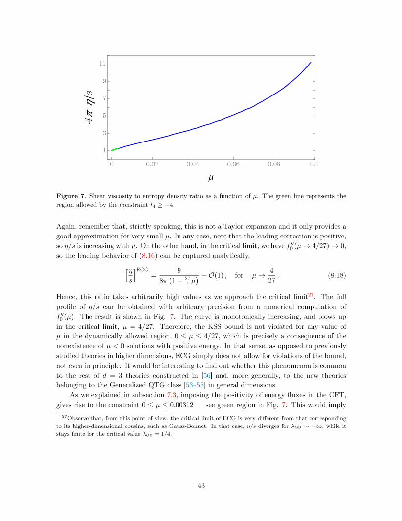
μ

πη/

Figure 7. Shear viscosity to entropy density ratio as a function of µ. The green line represents theregion allowed by the constraint t4 ≥ −4.

Again, remember that, strictly speaking, this is not a Taylor expansion and it only provides agood approximation for very small µ. In any case, note that the leading correction is positive,so η/s is increasing with µ. On the other hand, in the critical limit, we have f ′′0 (µ→ 4/27)→ 0,so the leading behavior of (8.16) can be captured analytically,[η

s

]ECG=

9

8π(1− 27

4 µ) +O(1) , for µ→ 4

27. (8.18)

Hence, this ratio takes arbitrarily high values as we approach the critical limit27. The fullprofile of η/s can be obtained with arbitrary precision from a numerical computation off ′′0 (µ). The result is shown in Fig. 7. The curve is monotonically increasing, and blows upin the critical limit, µ = 4/27. Therefore, the KSS bound is not violated for any value ofµ in the dynamically allowed region, 0 ≤ µ ≤ 4/27, which is precisely a consequence of thenonexistence of µ < 0 solutions with positive energy. In that sense, as opposed to previouslystudied theories in higher dimensions, ECG simply does not allow for violations of the bound,not even in principle. It would be interesting to find out whether this phenomenon is commonto the rest of d = 3 theories constructed in [56] and, more generally, to the new theoriesbelonging to the Generalized QTG class [53–55] in general dimensions.

As we explained in subsection 7.3, imposing the positivity of energy fluxes in the CFT,gives rise to the constraint 0 ≤ µ ≤ 0.00312 — see green region in Fig. 7. This would imply

27Observe that, from this point of view, the critical limit of ECG is very different from that correspondingto its higher-dimensional cousins, such as Gauss-Bonnet. In that case, η/s diverges for λGB → −∞, while itstays finite for the critical value λGB = 1/4.

– 43 –

a maximum possible value for η/s in ECG, given by[ηs

]ECG

max.' 1.253× 1

4π. (8.19)

From the results here, we can extract some general lessons regarding calculations of η/sin higher-curvature holographic CFTs. First, we have seen that the ECG result is highlynonperturbative in the gravitational coupling. There is in principle no reason to expect thisto be different for more general theories. The results found for Lovelock and QTG, polynomialin the gravitational couplings, are probably less generic — for those, the metric function f(r)

is determined by an algebraic equation, which is a highly exceptional property [54]. Besides,as we have seen, there may be regions of the parameter space for which the correspondingblack branes do not exist, even for arbitrarily small values of the couplings. None of thisis seen when working perturbatively in the gravitational couplings, which means that theresults obtained in that way must be taken carefully. This is a lesson which extends to mostcalculations in higher-curvature gravities.

9 Final comments

In this paper we have studied various aspects of d = 3 holographic ECG, which, as we haveargued, is a toy model of a nonsupersymmetric CFT (t4 6= 0) analogous to QTG in d = 4. Adetailed summary of our findings can be found in subsection 1.1. We close the paper with afew additional comments.

Throughout the paper, we have computed several universal charges characterizing the dualCFT. In Table 1 we have collected some of them, as well as their d = 4 QTG counterparts(with the Gauss-Bonnet coupling set to zero). For Einstein gravity, these are all proportionalto the only dimensionless quantity present in the Lagrangian, namely, L2/G. Just like for thehigher-dimensional examples previously considered, including QTG, the introduction of theECG coupling breaks this degeneracy, and all charges become independent from each other,in the sense that all possible ratios formed from them are µ-dependent. As we can see, thestress-tensor parameters have remarkably similar numerical coefficients in both theories whenexpressed in terms of the Einstein-gravity charges. The expressions for a∗ are also similar,whereas the ones for CS are considerably different, due to the appearance of an extra factorwhich vanishes in the critical limit for ECG. The differences extend to many other quantities,as we have tried to illustrate throughout the text, which suggests that similar analyses forother members of the Generalized QTG family [53–56] should be performed. In particular,it would be interesting to find out whether the highly-nonperturbative result for the shearviscosity over entropy density ratio extends to those theories, and whether violations of theKSS bound are also forbidden for them.

9.1 Generalized action, a∗ and holographic complexity?

In section 4, we proposed a new method for evaluating Euclidean on-shell actions for higher-order gravities whose linearized equations of motion on maximally symmetric backgrounds

– 44 –

CT CT · t4 CS a∗

Einstein Γ(d+2)

8(d−1)Γ(d/2)π(d+2)/2Ld−1

G 0 Γ(d+1)π(2d−1)/22d−3

Γ( d+12

)Γ(d/2)ddLd−1

Gπ(d−2)/2

8Γ(d/2)Ld−1

G

ECG (d = 3) (1− 3µf2∞)CE

T -3780µf2∞C

ET

(1− 27

4 µ)f2∞C

ES

(1 + 3µf2

∞)a∗E

QTG (d = 4) (1− 3µf2∞)CE

T 3780µf2∞C

ET f3

∞CES

(1 + 9µf2

∞)a∗E

Table 1. From left to right: stress-tensor two- and three-point function charges CT and CT · t4,thermal entropy charge CS, and universal contribution to the entanglement entropy across a sphericalregion, a∗, for holographic theories dual to Einstein gravity in d dimensions, ECG (d = 3) and Quasi-topological gravity (with vanishing Gauss-Bonnet coupling) in d = 4 [43].

are second order. Throughout the paper, we have performed several successful and highlynon-trivial checks of the proposal — see appendix B as well. It would be interesting toperform further studies of our generalized action (4.11) for other theories, such as higher-order Lovelock theories, QTG and its higher-order generalizations and, more generally, fortheories of the Generalized QTG type. One of the most striking aspects of (4.11) is that itavoids the — usually very challenging — problem of determining the correct generalization ofthe Gibbons-Hawking-York boundary term. At the same time, and somewhat surprisingly, itinvolves the universal charge a∗ controlling the EE of spherical regions in the correspondingdual CFT. This acts as a weight that changes from one theory to another.

As pointed out in [154], one of the open questions in the context of holographic complexity,is to determine what kind of universal information (if any) is encoded in the results obtainedusing the ‘complexity=volume’ [155, 156] and ‘complexity=action’ [157, 158] prescriptions.In order to do so, one possible venue would consist in studying the corresponding quantitiesfor holographic higher-order gravities. For those, the charge-degeneracy inherent to Einsteingravity (where all charges are proportional to L2/G) is broken, and one would hope to be ableto identify the nature of possible universal quantities28 appearing in holographic complexity.Our generalized action (4.11) suggests that a∗ may appear universally in some of these terms.Observe that complexity=action calculations require the introduction of additional terms inthe gravitational action when the boundary contains null pieces and joints — see [159] andreferences therein. In that case one can only speculate on whether a similar mechanism couldmake a∗ — or some other characteristic charge — appear in the corresponding generalizedterms for higher-order gravities.

28Certain ambiguities related to the normalization of affine parameters along null boundaries seem to pollutethe would-be universal terms in complexity=action calculations [154]. Dealing with those is an additionalchallenge.

– 45 –

Acknowledgments

We wish to thank Marco Baggio, Nikolay Bobev, Fridrik Gautason, Robie Hennigar, DiegoHofman, Carlos Hoyos, Robb Mann and Rob Myers for useful discussions. The work of PBwas supported by a postdoctoral fellowship from the National Science Foundation of Belgium(FWO). The work of PAC is funded by Fundación la Caixa through a “la Caixa - Severo Ochoa"International pre-doctoral grant. AR was supported by a “Centro de Excelencia InternacionalUAM/CSIC" FPI pre-doctoral grant and by a grant from the “Residencia de Estudiantes".PAC and AR were further supported by the MINECO/FEDER, UE grant FPA2015-66793-P,and from the “Centro de Excelencia Severo Ochoa" Program grant SEV-2016-0597. PAC alsothanks the Perimeter Institute “Visiting Graduate Fellows" program. Research at PerimeterInstitute is supported by the Government of Canada through the Department of Innovation,Science and Economic Development and by the Province of Ontario through the Ministry ofResearch, Innovation and Science.

A 〈TTT 〉 parameters from hq

In this appendix we show that the formulas in [126] for the twist operator scaling dimensions hqaround q = 1 can be used to obtain the exact values of the parameters t2 and t4 for holographicGauss-Bonnet in general dimensions, and for QTG in d = 4. The general-d version of (7.27)reads [126]

hqCT

= 2πd2

+1 Γ(d/2)

Γ(d+ 2)(q − 1) +

h′′q (1)

2CT

(q − 1)2 +O(q − 1)3 , (A.1)

where

h′′q (1)

CT

=− 2π1+d/2Γ(d/2)

(d− 1)3d(d+ 1)Γ(d+ 3)

[d(2d5 − 9d3 + 2d2 + 7d− 2

)+ (d− 2)(d− 3)(d+ 1)(d+ 2)(2d− 1)t2 + (d− 2)(7d3 − 19d2 − 8d+ 8)t4

].

(A.2)

This expression is valid for general holographic higher-order gravities, at least at leading orderin the gravitational couplings.

A.1 Gauss-Bonnet in arbitrary dimensions

In this case, the expression for the scaling dimension of twist operators is given by [25]

hqCT

=Γ(d/2)

4Γ(d+ 2)π1+d/2qxd−4

q (x2q − 1)

[d− 3− (d+ 1)x2

q + (d− 3)1− 2d−1

d−3λf∞

1− 2λf∞(x2q − 1)

],

(A.3)where xq satisfies the following quartic equation

x4qd−

2

qx3q − (d− 2)x2

q + λf∞

[4xqq− x4

qd+ d− 4

]= 0 . (A.4)

– 46 –

A Taylor expansion around q = 1 gives

xq = 1 +1

1− d(q − 1) +

d

(d− 1)3

−2d+ 3 + λf∞(4d− 10)

−2 + 4λf∞(q − 1)2 +O(q − 1)3 . (A.5)

Plugging this expansion into (A.3), we find

hqCT

=2Γ(d/2)π1+d/2

Γ(d+ 2)(q − 1) (A.6)

− (d− 1)Γ(d/2)π1+d/2

Γ(d+ 2)

[−1 + 4d− 2d2 + λf∞(6− 16d+ 4d2)

](q − 1)2 +O(q − 1)3 .

Comparing this with (A.1), we find that t2 and t4 should be given by

t2 =4d(d− 1)λf∞

(d− 2)(d− 3)(1− 2λf∞), t4 = 0 , (A.7)

which matches the exact nonperturbative result [33].

A.2 Quasi-topological gravity

In this case, the scaling dimension hq was obtained in [25] in terms of the charges a, c and t4of the theory as

hq =aq

4πx2q

(x2q − 1)

[x4q

(1− 5

c

a− 10

c

at4

)− x2

q

(1− c

a− 8

c

at4

)+ 2

c

at4

], (A.8)

where

c = π2 L3

8πG

(1− 2λf∞ − 3µf2

∞), (A.9)

a = π2 L3

8πG

(1− 6λf∞ + 9µf2

∞), (A.10)

t4 =3780µf2

∞1− 2λf∞ − 3µf2

∞, (A.11)

and where xq satisfies the following quartic equation

2x6q −

x5q

q− x4

q + 2λf∞x3q

(1

q− x3

q

)+ µf2

∞

(−1 +

3xqq− 2x6

q

)= 0 . (A.12)

Moreover, we have [43]

t2 =24f∞ (λ− 87µf∞)

1− 2λf∞ − 3µf2∞

, (A.13)

– 47 –

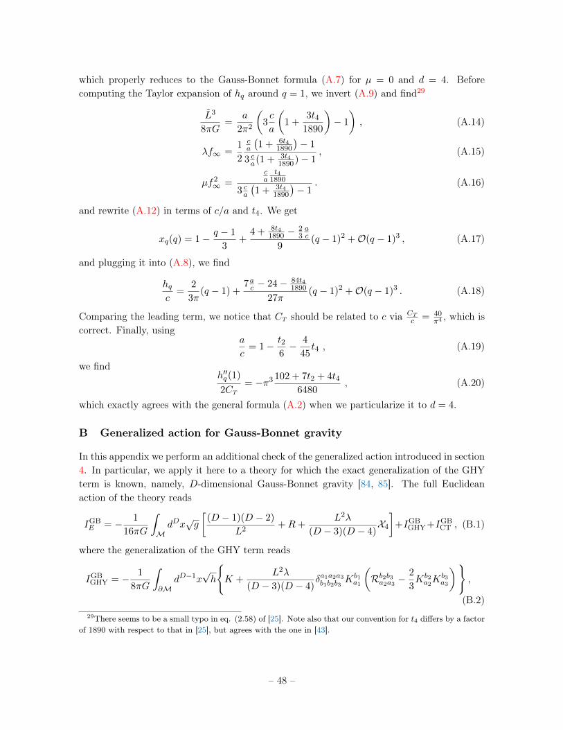
which properly reduces to the Gauss-Bonnet formula (A.7) for µ = 0 and d = 4. Beforecomputing the Taylor expansion of hq around q = 1, we invert (A.9) and find29

L3

8πG=

a

2π2

(3c

a

(1 +

3t41890

)− 1

), (A.14)

λf∞ =1

2

ca

(1 + 6t4

1890

)− 1

3 ca(1 + 3t41890)− 1

, (A.15)

µf2∞ =

ca

t41890

3 ca(1 + 3t4

1890

)− 1

. (A.16)

and rewrite (A.12) in terms of c/a and t4. We get

xq(q) = 1− q − 1

3+

4 + 8t41890 −

23ac

9(q − 1)2 +O(q − 1)3 , (A.17)

and plugging it into (A.8), we find

hqc

=2

3π(q − 1) +

7ac − 24− 84t41890

27π(q − 1)2 +O(q − 1)3 . (A.18)

Comparing the leading term, we notice that CT should be related to c via CTc = 40

π4 , which iscorrect. Finally, using

a

c= 1− t2

6− 4

45t4 , (A.19)

we findh′′q (1)

2CT

= −π3 102 + 7t2 + 4t46480

, (A.20)

which exactly agrees with the general formula (A.2) when we particularize it to d = 4.

B Generalized action for Gauss-Bonnet gravity

In this appendix we perform an additional check of the generalized action introduced in section4. In particular, we apply it here to a theory for which the exact generalization of the GHYterm is known, namely, D-dimensional Gauss-Bonnet gravity [84, 85]. The full Euclideanaction of the theory reads

IGBE = − 1

16πG

∫MdDx√g

[(D − 1)(D − 2)

L2+R+

L2λ

(D − 3)(D − 4)X4

]+IGB

GHY +IGBCT , (B.1)

where the generalization of the GHY term reads

IGBGHY = − 1

8πG

∫∂M

dD−1x√h

K +

L2λ

(D − 3)(D − 4)δa1a2a3b1b2b3

Kb1a1

(Rb2b3a2a3 −

2

3Kb2a2K

b3a3

),

(B.2)29There seems to be a small typo in eq. (2.58) of [25]. Note also that our convention for t4 differs by a factor

of 1890 with respect to that in [25], but agrees with the one in [43].

– 48 –

and the counterterms can be chosen as [72, 92–95]

IGBCT =

1

8πG

∫∂M

dD−1x√h

(D − 2)(f∞ + 2)

3f1/2∞ L

+L(3f∞ − 2)

2f3/2∞ (D − 3)

R+L3Θ[D − 6]

2f5/2∞ (D − 3)2(D − 5)

×[(2− f∞)

(RabRab −

D − 1

4(D − 2)R2

)− (D − 3)(1− f∞)

D − 4X4(h)

]+ . . .

. (B.3)

With these boundary contributions, the Gauss-Bonnet action functional is differentiable andfinite in AdS spaces. Since Gauss-Bonnet gravity has an Einstein-like spectrum in pure AdSD(in fact, in any background), our generalized GHY term should also be applicable to GBgravity, as long as the boundary consists only of asymptotically AdS pieces. The prescriptionin (4.11) gives the following result when applied to the Gauss-Bonnet Lagrangian,

IGBGGHY + IGB

GCT = −1− 2λf∞

D−2D−4

8πG

∫∂M

dD−1x√h

[K − D − 2

L− L

2(D − 3)R

− L3Θ[D − 6]

2(D − 3)2(D − 5)

(RabRab −

D − 1

4(D − 2)R2

)+ . . .

],

(B.4)

where we included a set of counterterms valid up toD = 7 and where L = L/√f∞. Recall that

the coefficient in front of the integral is proportional to the universal constant a∗ appearingin the EE across a spherical region, which for GB gravity reads

a∗ =

(1− 2λf∞

d− 1

d− 3

)Ld−1Ω(d−1)

16πG. (B.5)

In order to compare both boundary terms, let us consider a metric of the form

ds2 = f(r)dτ2 +dr2

f(r)+ r2dΣ2

k , (B.6)

where dΣ2k is the metric of a maximally symmetric space of curvature k = −1, 0, 1 and τ has

period β. For f(r) = f∞r2/L2 +k, the previous metric reduces to pure Euclidean AdSD, with

the boundary at r = +∞, which we regulate as r → L2/δ. Let us now switch on arbitraryradial perturbations

f(r) = f∞r2

L2+ k +

f1

r+f2

r2+f3

r3+ . . . . (B.7)

Evaluated at r → L2/δ, the boundary terms coming from both prescriptions yield, respectively

IGBGHY+CT =

βπ

4G

[(5f∞ − 6)L6

δ4+f1(5f∞ − 6)L2

f∞δ+

(5f∞ − 6)(4f2f∞ − 3L2k2

)8f2∞

+O(δ2)

],

IGBGGHY+GCT =

βπ

4G

[(5f∞ − 6)L6

δ4+f1(5f∞ − 6)L2

f∞δ+

(5f∞ − 6)(4f2f∞ − 3L2k2

)8f2∞

+O′(δ2)

].

This is, all divergent and finite terms are equal! The difference only appears in the decayingterms, which of course give no contribution to the action. For the sake of simplicity, we

– 49 –

evaluated the above expressions for D = 5, but it is straightforward to check that the samephenomenon happens in higher dimensions (with the expressions above we have checked D =

6, 7). Therefore, at least from a practical point of view, our generalized boundary term is asgood as the Gauss-Bonnet one when applied to asymptotically AdS spaces. We expect ourmethod to work also for general Lovelock gravities, as well as for QTG, and the rest of theoriesbelonging to the Einstein-like class in the classification of [64].

C Boundary terms in the two-point function

In this appendix we evaluate explicitly the boundary contribution in (4.24) for the metricperturbation considered in section 5. The sum of all boundary contributions appearing in(5.12), which includes the one coming from IECG

E Bulk in (5.6), as well as the generalized GHYterm and the counterterms in (4.24), reads

IECGE bdry = − 1

8πG

∫d3x

[1

2Γr + (1 + 3µf2

∞)√h

(K − 2

√f∞L− L

2√f∞R)]

, (C.1)

where Γr comes from integration by parts in the bulk action, and is given by

Γr =1√f∞

[− 2(4f∞ − 3)r3

L4+

4f∞ − 3

L4

(2r4φ∂rφ+ r3φ2

)+

(f∞ − 1)r5

L4(∂rφ)2 (C.2)

+ 6µf2∞

(−r

2(∂τφ)2 + r2∂rφ∂

2τφ)]

. (C.3)

The rest are the boundary terms in the action (4.24). The induced metric on a hypersurfaceof fixed r is

(3)ds2 =r2

L2

(dτ2 + dx2 + dy2 + 2dxdyφ(r, τ)

). (C.4)

At quadratic order in φ we have

√h =

r3

L3

(1− 1

2φ2

), R =

L2

2r2

(3(∂τφ)2 + 4φ∂2

τφ), K =

3√f∞L− r√f∞L

φ∂rφ . (C.5)

Then, we obtain at that order

IECGE bdry =

1

8πG

∫d3x

[3r3

L4√f∞

(1− f∞ + µf3∞)

(−1 +

φ2

2+ rφ∂rφ

)− 3(f∞ − 1)r5

2√f∞L4

(∂rφ)2

+r√f∞

((1 + 3µf2

∞)

(3

4(∂τφ)2 + φ∂2

τφ

)+

3µ

2f2∞(∂τφ)2

)− 3µf3/2

∞ r2∂rφ∂2τφ

].

(C.6)The first term vanishes because 1− f∞ + µf3

∞ = 0 is precisely the AdS4 embedding equation(2.4). Now it proves useful to perform the Fourier transformation of φ:

φ(r, τ) =1

2π

∫dpφ0(p)eipτHp(r) , (C.7)

– 50 –

with Hp(r) = e− L2|p|√

f∞r

(1 + L2|p|√

f∞r

). Then,

IECGE bdry =

VR2

16π2G

∫dpdqδ(q + p)φ0(p)φ0(q)

[− 3(f∞ − 1)r5

2√f∞L4

(∂rHp)2

+rH2

p√f∞

((1 + 3µf2

∞)

(−3

4pq − q2

)− 3µ

2f2∞pq

)+ 3µq2f3/2

∞ r2Hq∂rHp

].

(C.8)

Now, since ∂rHp ∼ 1/r3 , the first and last terms vanish for r → ∞. Then, we are left withthe final result

IECGE bdry = −VR2(1− 3µf2

∞)

64π2G√f∞

∫dpdqδ(q + p)φ0(p)φ0(q)p2rH2

p (r) , (C.9)

which appears in the main text.

References

[1] J. M. Maldacena, The Large N limit of superconformal field theories and supergravity, Int. J.Theor. Phys. 38 (1999) 1113–1133 [hep-th/9711200]. [Adv. Theor. Math. Phys.2,231(1998)].

[2] S. S. Gubser, I. R. Klebanov and A. M. Polyakov, Gauge theory correlators from noncriticalstring theory, Phys. Lett. B428 (1998) 105–114 [hep-th/9802109].

[3] E. Witten, Anti-de Sitter space and holography, Adv. Theor. Math. Phys. 2 (1998) 253–291[hep-th/9802150].

[4] M. T. Grisaru, A. E. M. van de Ven and D. Zanon, Four Loop beta Function for the N=1 andN=2 Supersymmetric Nonlinear Sigma Model in Two-Dimensions, Phys. Lett. B173 (1986)423–428.

[5] D. J. Gross and E. Witten, Superstring Modifications of Einstein’s Equations, Nucl. Phys.B277 (1986) 1.

[6] S. S. Gubser, I. R. Klebanov and A. A. Tseytlin, Coupling constant dependence in thethermodynamics of N=4 supersymmetric Yang-Mills theory, Nucl. Phys. B534 (1998) 202–222[hep-th/9805156].

[7] A. Buchel, J. T. Liu and A. O. Starinets, Coupling constant dependence of the shear viscosityin N=4 supersymmetric Yang-Mills theory, Nucl. Phys. B707 (2005) 56–68 [hep-th/0406264].

[8] A. Buchel, R. C. Myers and A. Sinha, Beyond eta/s = 1/4 pi, JHEP 03 (2009) 084[0812.2521].

[9] D. M. Hofman and J. Maldacena, Conformal collider physics: Energy and charge correlations,JHEP 05 (2008) 012 [0803.1467].

[10] D. M. Hofman, Higher Derivative Gravity, Causality and Positivity of Energy in a UVcomplete QFT, Nucl. Phys. B823 (2009) 174–194 [0907.1625].

[11] S. Nojiri and S. D. Odintsov, On the conformal anomaly from higher derivative gravity in AdS/ CFT correspondence, Int. J. Mod. Phys. A15 (2000) 413–428 [hep-th/9903033].

– 51 –

[12] M. Blau, K. S. Narain and E. Gava, On subleading contributions to the AdS / CFT traceanomaly, JHEP 09 (1999) 018 [hep-th/9904179].

[13] X. O. Camanho, J. D. Edelstein, J. Maldacena and A. Zhiboedov, Causality Constraints onCorrections to the Graviton Three-Point Coupling, JHEP 02 (2016) 020 [1407.5597].

[14] R. C. Myers and A. Sinha, Holographic c-theorems in arbitrary dimensions, JHEP 01 (2011)125 [1011.5819].

[15] R. C. Myers and A. Sinha, Seeing a c-theorem with holography, Phys. Rev. D82 (2010) 046006[1006.1263].

[16] M. Mezei, Entanglement entropy across a deformed sphere, Phys. Rev. D91 (2015), no. 4045038 [1411.7011].

[17] P. Bueno, R. C. Myers and W. Witczak-Krempa, Universality of corner entanglement inconformal field theories, Phys. Rev. Lett. 115 (2015) 021602 [1505.04804].

[18] P. Bueno and R. C. Myers, Corner contributions to holographic entanglement entropy, JHEP08 (2015) 068 [1505.07842].

[19] Y. Kats and P. Petrov, Effect of curvature squared corrections in AdS on the viscosity of thedual gauge theory, JHEP 01 (2009) 044 [0712.0743].

[20] M. Brigante, H. Liu, R. C. Myers, S. Shenker and S. Yaida, Viscosity Bound Violation inHigher Derivative Gravity, Phys. Rev. D77 (2008) 126006 [0712.0805].

[21] R. C. Myers, M. F. Paulos and A. Sinha, Quantum corrections to eta/s, Phys. Rev. D79(2009) 041901 [0806.2156].

[22] R.-G. Cai, Z.-Y. Nie and Y.-W. Sun, Shear Viscosity from Effective Couplings of Gravitons,Phys. Rev. D78 (2008) 126007 [0811.1665].

[23] X.-H. Ge, Y. Matsuo, F.-W. Shu, S.-J. Sin and T. Tsukioka, Viscosity Bound, CausalityViolation and Instability with Stringy Correction and Charge, JHEP 10 (2008) 009[0808.2354].

[24] P. Kovtun, D. T. Son and A. O. Starinets, Viscosity in strongly interacting quantum fieldtheories from black hole physics, Phys. Rev. Lett. 94 (2005) 111601 [hep-th/0405231].

[25] L.-Y. Hung, R. C. Myers, M. Smolkin and A. Yale, Holographic Calculations of Renyi Entropy,JHEP 12 (2011) 047 [1110.1084].

[26] L.-Y. Hung, R. C. Myers and M. Smolkin, Twist operators in higher dimensions, JHEP 10(2014) 178 [1407.6429].

[27] J. de Boer, M. Kulaxizi and A. Parnachev, Holographic Entanglement Entropy in LovelockGravities, JHEP 07 (2011) 109 [1101.5781].

[28] L. Bianchi, S. Chapman, X. Dong, D. A. Galante, M. Meineri and R. C. Myers, Shapedependence of holographic Rényi entropy in general dimensions, JHEP 11 (2016) 180[1607.07418].

[29] D. Lovelock, Divergence-free tensorial concomitants, aequationes mathematicae 4 (1970), no. 1127–138.

[30] D. Lovelock, The Einstein tensor and its generalizations, J. Math. Phys. 12 (1971) 498–501.

– 52 –

[31] X. O. Camanho and J. D. Edelstein, Causality constraints in AdS/CFT from conformalcollider physics and Gauss-Bonnet gravity, JHEP 04 (2010) 007 [0911.3160].

[32] J. de Boer, M. Kulaxizi and A. Parnachev, AdS(7)/CFT(6), Gauss-Bonnet Gravity, andViscosity Bound, JHEP 03 (2010) 087 [0910.5347].

[33] A. Buchel, J. Escobedo, R. C. Myers, M. F. Paulos, A. Sinha and M. Smolkin, Holographic GBgravity in arbitrary dimensions, JHEP 03 (2010) 111 [0911.4257].

[34] J. de Boer, M. Kulaxizi and A. Parnachev, Holographic Lovelock Gravities and Black Holes,JHEP 06 (2010) 008 [0912.1877].

[35] X. O. Camanho and J. D. Edelstein, Causality in AdS/CFT and Lovelock theory, JHEP 06(2010) 099 [0912.1944].

[36] S. Grozdanov and A. O. Starinets, On the universal identity in second order hydrodynamics,JHEP 03 (2015) 007 [1412.5685].

[37] S. Grozdanov and A. O. Starinets, Second-order transport, quasinormal modes andzero-viscosity limit in the Gauss-Bonnet holographic fluid, JHEP 03 (2017) 166 [1611.07053].

[38] T. Andrade, J. Casalderrey-Solana and A. Ficnar, Holographic Isotropisation in Gauss-BonnetGravity, JHEP 02 (2017) 016 [1610.08987].

[39] R. A. Konoplya and A. Zhidenko, Quasinormal modes of Gauss-Bonnet-AdS black holes:towards holographic description of finite coupling, JHEP 09 (2017) 139 [1705.07732].

[40] R. C. Myers and B. Robinson, Black Holes in Quasi-topological Gravity, JHEP 08 (2010) 067[1003.5357].

[41] J. Oliva and S. Ray, A new cubic theory of gravity in five dimensions: Black hole, Birkhoff’stheorem and C-function, Class. Quant. Grav. 27 (2010) 225002 [1003.4773].

[42] X. O. Camanho, J. D. Edelstein and J. M. Sánchez De Santos, Lovelock theory and theAdS/CFT correspondence, Gen. Rel. Grav. 46 (2014) 1637 [1309.6483].

[43] R. C. Myers, M. F. Paulos and A. Sinha, Holographic studies of quasi-topological gravity,JHEP 08 (2010) 035 [1004.2055].

[44] M. Kulaxizi and A. Parnachev, Supersymmetry Constraints in Holographic Gravities, Phys.Rev. D82 (2010) 066001 [0912.4244].

[45] O. Aharony, O. Bergman, D. L. Jafferis and J. Maldacena, N=6 superconformalChern-Simons-matter theories, M2-branes and their gravity duals, JHEP 10 (2008) 091[0806.1218].

[46] O. Aharony, O. Bergman and D. L. Jafferis, Fractional M2-branes, JHEP 11 (2008) 043[0807.4924].

[47] I. R. Klebanov and A. M. Polyakov, AdS dual of the critical O(N) vector model, Phys. Lett.B550 (2002) 213–219 [hep-th/0210114].

[48] R. G. Leigh and A. C. Petkou, Holography of the N=1 higher spin theory on AdS(4), JHEP 06(2003) 011 [hep-th/0304217].

[49] O. Aharony, G. Gur-Ari and R. Yacoby, d=3 Bosonic Vector Models Coupled to Chern-SimonsGauge Theories, JHEP 03 (2012) 037 [1110.4382].

– 53 –

[50] P. Bueno and P. A. Cano, Einsteinian cubic gravity, Phys. Rev. D94 (2016), no. 10 104005[1607.06463].

[51] R. A. Hennigar and R. B. Mann, Black holes in Einsteinian cubic gravity, Phys. Rev. D95(2017), no. 6 064055 [1610.06675].

[52] P. Bueno and P. A. Cano, Four-dimensional black holes in Einsteinian cubic gravity, Phys.Rev. D94 (2016), no. 12 124051 [1610.08019].

[53] R. A. Hennigar, D. Kubizňák and R. B. Mann, Generalized quasitopological gravity, Phys. Rev.D95 (2017), no. 10 104042 [1703.01631].

[54] P. Bueno and P. A. Cano, On black holes in higher-derivative gravities, Class. Quant. Grav. 34(2017), no. 17 175008 [1703.04625].

[55] J. Ahmed, R. A. Hennigar, R. B. Mann and M. Mir, Quintessential Quartic Quasi-topologicalQuartet, JHEP 05 (2017) 134 [1703.11007].

[56] P. Bueno and P. A. Cano, Universal black hole stability in four dimensions, Phys. Rev. D96(2017), no. 2 024034 [1704.02967].

[57] M. H. Dehghani, A. Bazrafshan, R. B. Mann, M. R. Mehdizadeh, M. Ghanaatian and M. H.Vahidinia, Black Holes in Quartic Quasitopological Gravity, Phys. Rev. D85 (2012) 104009[1109.4708].

[58] M. H. Dehghani and M. H. Vahidinia, Quartic Quasi-topological Gravity, Black Holes andHolography, JHEP 10 (2013) 210 [1307.0330].

[59] A. Cisterna, L. Guajardo, M. Hassaine and J. Oliva, Quintic quasi-topological gravity, JHEP04 (2017) 066 [1702.04676].

[60] R. A. Hennigar, Criticality for charged black branes, JHEP 09 (2017) 082 [1705.07094].

[61] X.-H. Feng, H. Huang, Z.-F. Mai and H. Lu, Bounce Universe and Black Holes from CriticalEinsteinian Cubic Gravity, Phys. Rev. D96 (2017), no. 10 104034 [1707.06308].

[62] R. A. Hennigar, M. B. J. Poshteh and R. B. Mann, Shadows, Signals, and Stability inEinsteinian Cubic Gravity, 1801.03223.

[63] A. Dey, P. Roy and T. Sarkar, On Holographic Rényi Entropy in Some Modified Theories ofGravity, 1609.02290.

[64] P. Bueno, P. A. Cano, V. S. Min and M. R. Visser, Aspects of general higher-order gravities,Phys. Rev. D95 (2017), no. 4 044010 [1610.08519].

[65] L. F. Abbott and S. Deser, Stability of Gravity with a Cosmological Constant, Nucl. Phys.B195 (1982) 76–96.

[66] S. Deser and B. Tekin, Energy in generic higher curvature gravity theories, Phys. Rev. D67(2003) 084009 [hep-th/0212292].

[67] J. T. Wheeler, Symmetric Solutions to the Gauss-Bonnet Extended Einstein Equations, Nucl.Phys. B268 (1986) 737–746.

[68] J. T. Wheeler, Symmetric Solutions to the Maximally Gauss-Bonnet Extended EinsteinEquations, Nucl. Phys. B273 (1986) 732.

– 54 –

[69] D. G. Boulware and S. Deser, String Generated Gravity Models, Phys. Rev. Lett. 55 (1985)2656.

[70] R.-G. Cai, Gauss-Bonnet black holes in AdS spaces, Phys. Rev. D65 (2002) 084014[hep-th/0109133].

[71] M. H. Dehghani and R. Pourhasan, Thermodynamic instability of black holes of third orderLovelock gravity, Phys. Rev. D79 (2009) 064015 [0903.4260].

[72] R. Emparan, C. V. Johnson and R. C. Myers, Surface terms as counterterms in the AdS /CFT correspondence, Phys. Rev. D60 (1999) 104001 [hep-th/9903238].

[73] M. Banados, C. Teitelboim and J. Zanelli, The Black hole in three-dimensional space-time,Phys. Rev. Lett. 69 (1992) 1849–1851 [hep-th/9204099].

[74] R. A. Davison and B. Goutéraux, Momentum dissipation and effective theories of coherent andincoherent transport, JHEP 01 (2015) 039 [1411.1062].

[75] G. Compère, The Kerr/CFT correspondence and its extensions, Living Rev. Rel. 15 (2012) 11[1203.3561]. [Living Rev. Rel.20,no.1,1(2017)].

[76] N. Ohta and T. Torii, Global Structure of Black Holes in String Theory with Gauss-BonnetCorrection in Various Dimensions, Prog. Theor. Phys. 124 (2010) 207–225 [1004.2779].

[77] A. Karasu, E. Kenar and B. Tekin, Minimal extension of Einstein’s theory: The quarticgravity, Phys. Rev. D93 (2016), no. 8 084040 [1602.02567].

[78] P. Bueno, P. A. Cano, A. O. Lasso and P. F. Ramirez, f(Lovelock) theories of gravity, JHEP04 (2016) 028 [1602.07310].

[79] Y.-Z. Li, H.-S. Liu and H. Lu, Quasi-Topological Ricci Polynomial Gravities, 1708.07198.

[80] Y.-Z. Li, H. Lu and J.-B. Wu, Causality and a-theorem Constraints on Ricci Polynomial andRiemann Cubic Gravities, 1711.03650.

[81] J. W. York, Jr., Role of conformal three geometry in the dynamics of gravitation, Phys. Rev.Lett. 28 (1972) 1082–1085.

[82] G. W. Gibbons and S. W. Hawking, Action Integrals and Partition Functions in QuantumGravity, Phys. Rev. D15 (1977) 2752–2756.

[83] J. Smolic and M. Taylor, Higher derivative effects for 4d AdS gravity, JHEP 06 (2013) 096[1301.5205].

[84] C. Teitelboim and J. Zanelli, Dimensionally continued topological gravitation theory inHamiltonian form, Class. Quant. Grav. 4 (1987) L125.

[85] R. C. Myers, Higher Derivative Gravity, Surface Terms and String Theory, Phys. Rev. D36(1987) 392.

[86] M. S. Madsen and J. D. Barrow, De Sitter Ground States and Boundary Terms in GeneralizedGravity, Nucl. Phys. B323 (1989) 242–252.

[87] E. Dyer and K. Hinterbichler, Boundary Terms, Variational Principles and Higher DerivativeModified Gravity, Phys. Rev. D79 (2009) 024028 [0809.4033].

[88] A. Guarnizo, L. Castaneda and J. M. Tejeiro, Boundary Term in Metric f(R) Gravity: FieldEquations in the Metric Formalism, Gen. Rel. Grav. 42 (2010) 2713–2728 [1002.0617].

– 55 –

[89] N. Deruelle, M. Sasaki, Y. Sendouda and D. Yamauchi, Hamiltonian formulation off(Riemann) theories of gravity, Prog. Theor. Phys. 123 (2010) 169–185 [0908.0679].

[90] A. Teimouri, S. Talaganis, J. Edholm and A. Mazumdar, Generalised Boundary Terms forHigher Derivative Theories of Gravity, JHEP 08 (2016) 144 [1606.01911].

[91] A. Yale, Simple counterterms for asymptotically AdS spacetimes in Lovelock gravity, Phys.Rev. D84 (2011) 104036 [1107.1250].

[92] R. B. Mann, Misner string entropy, Phys. Rev. D60 (1999) 104047 [hep-th/9903229].

[93] V. Balasubramanian and P. Kraus, A Stress tensor for Anti-de Sitter gravity, Commun. Math.Phys. 208 (1999) 413–428 [hep-th/9902121].

[94] Y. Brihaye and E. Radu, Black objects in the Einstein-Gauss-Bonnet theory with negativecosmological constant and the boundary counterterm method, JHEP 09 (2008) 006 [0806.1396].

[95] D. Astefanesei, N. Banerjee and S. Dutta, (Un)attractor black holes in higher derivative AdSgravity, JHEP 11 (2008) 070 [0806.1334].

[96] H. Casini, M. Huerta and R. C. Myers, Towards a derivation of holographic entanglemententropy, JHEP 05 (2011) 036 [1102.0440].

[97] C. Imbimbo, A. Schwimmer, S. Theisen and S. Yankielowicz, Diffeomorphisms and holographicanomalies, Class. Quant. Grav. 17 (2000) 1129–1138 [hep-th/9910267].

[98] A. Schwimmer and S. Theisen, Entanglement Entropy, Trace Anomalies and Holography, Nucl.Phys. B801 (2008) 1–24 [0802.1017].

[99] M. H. Dehghani and M. H. Vahidinia, Surface Terms of Quasitopological Gravity andThermodynamics of Charged Rotating Black Branes, Phys. Rev. D84 (2011) 084044[1108.4235].

[100] H. Osborn and A. C. Petkou, Implications of conformal invariance in field theories for generaldimensions, Annals Phys. 231 (1994) 311–362 [hep-th/9307010].

[101] Y. Huh and P. Strack, Stress tensor and current correlators of interacting conformal fieldtheories in 2+1 dimensions: Fermionic Dirac matter coupled to U(1) gauge field, JHEP 01(2015) 147 [1410.1902]. [Erratum: JHEP03,054(2016)].

[102] K. Diab, L. Fei, S. Giombi, I. R. Klebanov and G. Tarnopolsky, On CJ and CT in theGross–Neveu and O(N) models, J. Phys. A49 (2016), no. 40 405402 [1601.07198].

[103] S. Giombi, G. Tarnopolsky and I. R. Klebanov, On CJ and CT in Conformal QED, JHEP 08(2016) 156 [1602.01076].

[104] A. B. Zamolodchikov, Irreversibility of the Flux of the Renormalization Group in a 2D FieldTheory, JETP Lett. 43 (1986) 730–732. [Pisma Zh. Eksp. Teor. Fiz.43,565(1986)].

[105] T. Nishioka and K. Yonekura, On RG Flow of tauRR for Supersymmetric Field Theories inThree-Dimensions, JHEP 05 (2013) 165 [1303.1522].

[106] E. Perlmutter, A universal feature of CFT Rényi entropy, JHEP 03 (2014) 117 [1308.1083].

[107] W. Witczak-Krempa, Constraining Quantum Critical Dynamics: (2+1)D Ising Model andBeyond, Phys. Rev. Lett. 114 (2015) 177201 [1501.03495].

– 56 –

[108] A. Lucas, T. Sierens and W. Witczak-Krempa, Quantum critical response: from conformalperturbation theory to holography, JHEP 07 (2017) 149 [1704.05461].

[109] C. Closset, T. T. Dumitrescu, G. Festuccia and Z. Komargodski, Supersymmetric FieldTheories on Three-Manifolds, JHEP 05 (2013) 017 [1212.3388].

[110] N. Bobev, P. Bueno and Y. Vreys, Comments on Squashed-sphere Partition Functions, JHEP07 (2017) 093 [1705.00292].

[111] S. Fischetti and T. Wiseman, On universality of holographic results for (2 + 1)-dimensionalCFTs on curved spacetimes, JHEP 12 (2017) 133 [1707.03825].

[112] H. Liu and A. A. Tseytlin, D = 4 superYang-Mills, D = 5 gauged supergravity, and D = 4conformal supergravity, Nucl. Phys. B533 (1998) 88–108 [hep-th/9804083].

[113] R. M. Wald, Black hole entropy is the Noether charge, Phys. Rev. D48 (1993) 3427–3431[gr-qc/9307038].

[114] V. Iyer and R. M. Wald, Some properties of Noether charge and a proposal for dynamical blackhole entropy, Phys. Rev. D50 (1994) 846–864 [gr-qc/9403028].

[115] X. O. Camanho and J. D. Edelstein, A Lovelock black hole bestiary, Class. Quant. Grav. 30(2013) 035009 [1103.3669].

[116] E. Witten, Anti-de Sitter space, thermal phase transition, and confinement in gauge theories,Adv. Theor. Math. Phys. 2 (1998) 505–532 [hep-th/9803131].

[117] G. T. Horowitz and R. C. Myers, The AdS / CFT correspondence and a new positive energyconjecture for general relativity, Phys. Rev. D59 (1998) 026005 [hep-th/9808079].

[118] S. W. Hawking and D. N. Page, Thermodynamics of Black Holes in anti-De Sitter Space,Commun. Math. Phys. 87 (1983) 577.

[119] Y. M. Cho and I. P. Neupane, Anti-de Sitter black holes, thermal phase transition andholography in higher curvature gravity, Phys. Rev. D66 (2002) 024044 [hep-th/0202140].

[120] Y. S. Myung, No Hawking-Page phase transition in three dimensions, Phys. Lett. B624 (2005)297–303 [hep-th/0506096].

[121] X. O. Camanho, J. D. Edelstein, G. Giribet and A. Gomberoff, Generalized phase transitionsin Lovelock gravity, Phys. Rev. D90 (2014), no. 6 064028 [1311.6768].

[122] A. Rényi, On measures of entropy and information, Proceedings of the Fourth BerkeleySymposium on Mathematical Statistics and Probability, Volume 1: Contributions to the Theoryof Statistics (1961) 547–561.

[123] A. Rényi, On the foundations of information theory, Revue de l’Institut International deStatistique / Review of the International Statistical Institute 33 (1965), no. 1 1–14.

[124] I. R. Klebanov, S. S. Pufu, S. Sachdev and B. R. Safdi, Renyi Entropies for Free FieldTheories, JHEP 04 (2012) 074 [1111.6290].

[125] N. Laflorencie, Quantum entanglement in condensed matter systems, Phys. Rept. 646 (2016)1–59 [1512.03388].

[126] C.-S. Chu and R.-X. Miao, Universality in the shape dependence of holographic Rényi entropyfor general higher derivative gravity, JHEP 12 (2016) 036 [1608.00328].

– 57 –

[127] S. Ryu and T. Takayanagi, Holographic derivation of entanglement entropy from AdS/CFT,Phys. Rev. Lett. 96 (2006) 181602 [hep-th/0603001].

[128] S. Ryu and T. Takayanagi, Aspects of Holographic Entanglement Entropy, JHEP 08 (2006)045 [hep-th/0605073].

[129] D. V. Fursaev, A. Patrushev and S. N. Solodukhin, Distributional Geometry of SquashedCones, Phys. Rev. D88 (2013), no. 4 044054 [1306.4000].

[130] X. Dong, Holographic Entanglement Entropy for General Higher Derivative Gravity, JHEP 01(2014) 044 [1310.5713].

[131] J. Camps, Generalized entropy and higher derivative Gravity, JHEP 03 (2014) 070[1310.6659].

[132] V. G. M. Puletti and R. Pourhasan, Non-analyticity of holographic Rényi entropy in Lovelockgravity, JHEP 08 (2017) 002 [1704.08731].

[133] D. A. Galante and R. C. Myers, Holographic Renyi entropies at finite coupling, JHEP 08(2013) 063 [1305.7191].

[134] A. Belin, A. Maloney and S. Matsuura, Holographic Phases of Renyi Entropies, JHEP 12(2013) 050 [1306.2640].

[135] H. Casini, M. Huerta, R. C. Myers and A. Yale, Mutual information and the F-theorem, JHEP10 (2015) 003 [1506.06195].

[136] B. Swingle, Structure of entanglement in regulated Lorentz invariant field theories, 1304.6402.

[137] P. Bueno, R. C. Myers and W. Witczak-Krempa, Universal corner entanglement from twistoperators, JHEP 09 (2015) 091 [1507.06997].

[138] P. Calabrese and J. L. Cardy, Entanglement entropy and quantum field theory, J. Stat. Mech.0406 (2004) P06002 [hep-th/0405152].

[139] B. Swingle, Mutual information and the structure of entanglement in quantum field theory,1010.4038.

[140] S. Giombi, S. Prakash and X. Yin, A Note on CFT Correlators in Three Dimensions, JHEP07 (2013) 105 [1104.4317].

[141] J. M. Maldacena and G. L. Pimentel, On graviton non-Gaussianities during inflation, JHEP09 (2011) 045 [1104.2846].

[142] S. D. Chowdhury, J. R. David and S. Prakash, Constraints on parity violating conformal fieldtheories in d = 3, 1707.03007.

[143] S. Cremonini, The Shear Viscosity to Entropy Ratio: A Status Report, Mod. Phys. Lett. B25(2011) 1867–1888 [1108.0677].

[144] X. O. Camanho, J. D. Edelstein and M. F. Paulos, Lovelock theories, holography and the fateof the viscosity bound, JHEP 05 (2011) 127 [1010.1682].

[145] I. Fouxon, G. Betschart and J. D. Bekenstein, The Bound on viscosity and the generalizedsecond law of thermodynamics, Phys. Rev. D77 (2008) 024016 [0710.1429].

[146] M. F. Paulos, Transport coefficients, membrane couplings and universality at extremality,JHEP 02 (2010) 067 [0910.4602].

– 58 –

[147] G. Pasini and C. S. Shahbazi, Five-dimensional null and time-like supersymmetric geometries,Class. Quant. Grav. 33 (2016), no. 17 175003 [1512.02211].

[148] Z.-Y. Fan, Note on Noether charge and holographic transports, 1801.07870.

[149] X.-H. Ge and S.-J. Sin, Shear viscosity, instability and the upper bound of the Gauss-Bonnetcoupling constant, JHEP 05 (2009) 051 [0903.2527].

[150] R. Brustein and A. J. M. Medved, The Ratio of shear viscosity to entropy density ingeneralized theories of gravity, Phys. Rev. D79 (2009) 021901 [0808.3498].

[151] F.-W. Shu, The Quantum Viscosity Bound In Lovelock Gravity, Phys. Lett. B685 (2010)325–328 [0910.0607].

[152] S. Grozdanov and A. O. Starinets, Zero-viscosity limit in a holographic Gauss–Bonnet liquid,Theor. Math. Phys. 182 (2015), no. 1 61–73. [Teor. Mat. Fiz.182,no.1,76(2014)].

[153] S. Parvizi and M. Sadeghi, Holographic Aspects of a Higher Curvature Massive Gravity,1704.00441.

[154] D. Carmi, R. C. Myers and P. Rath, Comments on Holographic Complexity, JHEP 03 (2017)118 [1612.00433].

[155] L. Susskind, Computational Complexity and Black Hole Horizons, Fortsch. Phys. 64 (2016)44–48 [1403.5695]. [Fortsch. Phys.64,24(2016)].

[156] D. Stanford and L. Susskind, Complexity and Shock Wave Geometries, Phys. Rev. D90 (2014),no. 12 126007 [1406.2678].

[157] A. R. Brown, D. A. Roberts, L. Susskind, B. Swingle and Y. Zhao, Holographic ComplexityEquals Bulk Action?, Phys. Rev. Lett. 116 (2016), no. 19 191301 [1509.07876].

[158] A. R. Brown, D. A. Roberts, L. Susskind, B. Swingle and Y. Zhao, Complexity, action, andblack holes, Phys. Rev. D93 (2016), no. 8 086006 [1512.04993].

[159] L. Lehner, R. C. Myers, E. Poisson and R. D. Sorkin, Gravitational action with nullboundaries, Phys. Rev. D94 (2016), no. 8 084046 [1609.00207].

– 59 –