hjb equation and statistical arbitrage applied to high
TRANSCRIPT

University of Central Florida University of Central Florida
STARS STARS
Electronic Theses and Dissertations, 2004-2019
2013
Hjb Equation And Statistical Arbitrage Applied To High Frequency Hjb Equation And Statistical Arbitrage Applied To High Frequency
Trading Trading
Yonggi Park University of Central Florida
Part of the Mathematics Commons
Find similar works at: https://stars.library.ucf.edu/etd
University of Central Florida Libraries http://library.ucf.edu
This Masters Thesis (Open Access) is brought to you for free and open access by STARS. It has been accepted for
inclusion in Electronic Theses and Dissertations, 2004-2019 by an authorized administrator of STARS. For more
information, please contact [email protected].
STARS Citation STARS Citation Park, Yonggi, "Hjb Equation And Statistical Arbitrage Applied To High Frequency Trading" (2013). Electronic Theses and Dissertations, 2004-2019. 2674. https://stars.library.ucf.edu/etd/2674

HJB EQUATION AND STATISTICAL ARBITRAGE APPLIED TO HIGH FREQUENCYTRADING
by
YONGGI PARKM.S. University of Central Oklahoma, 2009
A thesis submitted in partial fulfilment of the requirementsfor the degree of Master of Sciencein the Department of Mathematics
in the College of Scienceat the University of Central Florida
Orlando, Florida
Summer Term2013
Major Professor: Jiongmin Yong

c© 2013Yonggi Park
ii

ABSTRACT
In this thesis we investigate some properties of market making and statistical arbitrage applied
to High Frequency Trading (HFT). Using the Hamilton-Jacobi-Bellman(HJB) model developed
by Guilbaud, Fabien and Pham, Huyen in 2012, we studied how market making works to obtain
optimal strategy during limit order and market order. Also we develop the best investment strategy
through Moving Average, Exponential Moving Average, Relative Strength Index, Sharpe Ratio.
iii

ACKNOWLEDGMENTS
First of all, I want to express my deepest gratitude to my supervisor Dr. Jiongmin Yong for helping
me out when I most need. He has been truly inspirational, has also been so generous in allowing
me to explore freely, but at the same time, always helped me to stay focused!
Thanks to Dr. Jason Swanson and Dr. Zhisheng Shuai for their guidence, dedication and support
through all my time at UCF.
Thanks to Sunghyun Jo for his colaboration in the example of LOB section of this work and
through his web contents for high frequency trading.
Thanks to Tian Xiao Wang for his collaboration in the interesting discussions we have on Optimal
Control.
Thanks to Roman Krylov for his collaboration in Latex learning.
iv

TABLE OF CONTENTS
LIST OF FIGURES . . . . . . . . . . . . . . . . . . . . . . . . . . . . . . . . . . . . . . vii
LIST OF TABLES . . . . . . . . . . . . . . . . . . . . . . . . . . . . . . . . . . . . . . . vii
CHAPTER 1: INTRODUCTION . . . . . . . . . . . . . . . . . . . . . . . . . . . . . . . 1
Definition . . . . . . . . . . . . . . . . . . . . . . . . . . . . . . . . . . . . . . . . . . 3
Limit order/Market order . . . . . . . . . . . . . . . . . . . . . . . . . . . . . . . 3
Bid/ask price . . . . . . . . . . . . . . . . . . . . . . . . . . . . . . . . . . . . . 3
Market maker . . . . . . . . . . . . . . . . . . . . . . . . . . . . . . . . . . . . . 4
The market maker’s spread . . . . . . . . . . . . . . . . . . . . . . . . . . . . . . 4
Midprice . . . . . . . . . . . . . . . . . . . . . . . . . . . . . . . . . . . . . . . . 4
Quotes . . . . . . . . . . . . . . . . . . . . . . . . . . . . . . . . . . . . . . . . . 5
Market making . . . . . . . . . . . . . . . . . . . . . . . . . . . . . . . . . . . . 5
Latency and Low latency . . . . . . . . . . . . . . . . . . . . . . . . . . . . . . . 5
Ultra-low latency . . . . . . . . . . . . . . . . . . . . . . . . . . . . . . . . . . . 6
Shelf life . . . . . . . . . . . . . . . . . . . . . . . . . . . . . . . . . . . . . . . . 6
Direct Market Access (DMA) . . . . . . . . . . . . . . . . . . . . . . . . . . . . 6
v

The characteristics of high frequency trading . . . . . . . . . . . . . . . . . . . . . . . . 6
The features of HFT . . . . . . . . . . . . . . . . . . . . . . . . . . . . . . . . . . 6
Low Latency, Ultra-Low Latency Direct Market Access(ULLDMA) . . . . 7
Multiple asset classes and exchanges . . . . . . . . . . . . . . . . . . . . 8
Limited shelf life or Short holding position period . . . . . . . . . . . . . 8
The advantages of HFT . . . . . . . . . . . . . . . . . . . . . . . . . . . . . . . . 9
Bid-ask spread . . . . . . . . . . . . . . . . . . . . . . . . . . . . . . . . 9
Liquidity . . . . . . . . . . . . . . . . . . . . . . . . . . . . . . . . . . . 9
Speed . . . . . . . . . . . . . . . . . . . . . . . . . . . . . . . . . . . . . 9
Volatility . . . . . . . . . . . . . . . . . . . . . . . . . . . . . . . . . . . 10
Increased market efficiency . . . . . . . . . . . . . . . . . . . . . . . . . 10
Fee . . . . . . . . . . . . . . . . . . . . . . . . . . . . . . . . . . . . . . 10
CHAPTER 2: INTRODUCTION OF MARKET MAKING . . . . . . . . . . . . . . . . . 11
Features of market making strategies . . . . . . . . . . . . . . . . . . . . . . . . . . . . 11
Market-making Model . . . . . . . . . . . . . . . . . . . . . . . . . . . . . . . . . . . 12
Limit Order strategy . . . . . . . . . . . . . . . . . . . . . . . . . . . . . . . . . 15
Market order strategies . . . . . . . . . . . . . . . . . . . . . . . . . . . . . . . . 21
vi
Optimal control problem . . . . . . . . . . . . . . . . . . . . . . . . . . . . . . . . . . 23
Dynamic programming equation (DPE) . . . . . . . . . . . . . . . . . . . . . . . 24
CHAPTER 3: STATISTICAL ARBITRAGE . . . . . . . . . . . . . . . . . . . . . . . . . 30
Definition . . . . . . . . . . . . . . . . . . . . . . . . . . . . . . . . . . . . . . . . . . 30
Pairs trading . . . . . . . . . . . . . . . . . . . . . . . . . . . . . . . . . . . . . . 30
Moving Average (MA) . . . . . . . . . . . . . . . . . . . . . . . . . . . . . . . . . . . 33
Exponential Moving Average (EMA) . . . . . . . . . . . . . . . . . . . . . . . . . . . . 34
Relative Strength Index (RSI) . . . . . . . . . . . . . . . . . . . . . . . . . . . . . . . . 36
Sharpe Ratio . . . . . . . . . . . . . . . . . . . . . . . . . . . . . . . . . . . . . . . . . 37
CHAPTER 4: CONCLUSION . . . . . . . . . . . . . . . . . . . . . . . . . . . . . . . . 44
APPENDIX : CODE FOR FIGURES OF CHAPTER 3 . . . . . . . . . . . . . . . . . . 45
LIST OF REFERENCES . . . . . . . . . . . . . . . . . . . . . . . . . . . . . . . . . . . 48
vii

CHAPTER 1: INTRODUCTION
Let us begin with a classical stock trading scenario. Suppose, at timet0, investor A wants to sell
one share of a given stock and investor B wants to buy one share of this stock at timet > t0.
Investors A and B do not meet directly, and a person, called a market maker, labeled by C, will buy
the stock from A at timet at price, saypb, called a bid price, and will sell it to investor B at price,
saypa, called an ask price, withpa > pb. The differencepa − pb > 0 is called the bid-ask spread.
Usually traders might make several trades per day, or per week (even per month).
Nowadays, without the formal designation, any trading firms can play a role as market mak-
ers by using (swift electronic) High frequency trading (HFT, for short) system through elec-
tronic exchanges like Nasdaq’s Inet, an electronic trading platform acquired by NASDAQ in
2005([26],[24],[11]).
More precisely, anyone can post the number of shares`b of the stock with the bid priceqb at which
she would like to buy, which is called a limit bid order and at the same time she can post the
number of sharesa of the stock with the ask priceqa at which she would like to sell, which is
called an limit ask order. The postings are made by numerous individuals from a list which is
called the limit order book (LOB, for short). People submit limit bid order and limit ask order
simultaneously, and gain a possible profit from the bid-ask spread, which was the profit of market
maker in classical trading. Unlike classical traders, HFT traders have information in the same level
as a market maker. In other words, all traders play a role as market makers, which means that
passive investors in classical trading are changed to active investors in HFT. Since trading firms
are acting as market makers in HFT by making limit orders, we refer to the algorithms associated
with limit orders as market making algorithms.
The introduction of some advanced tools involving computers allows the trading speed to be faster
1
and faster. Then, trading can be made more and more frequent. Unlike classical trading, HFT
may hold an investment position for only seconds, or fractions of a second and uses the computer
trading in and out of positions of thousands or tens of thousands of time a day, and the terminology
of high frequency is come from these huge transaction number([45]).
Long-term investors look for chances over a period of weeks, months, or years, but HFT traders
struggle on a rapid basis with other HFT traders, and struggle for very tiny, persistent profits
([29],[40]). High frequency traders aim to get only a fraction of a penny per stock or currency unit
on each trade, and move in and out of short-term positions many times each day. Fractions of a
penny are aggregated fast and produce vary huge profits at the end of each day ([24]). In finance,
leverage means any technique to multiply gains and losses, and general ways to get leverage are
borrowing money, buying fixed assets and using derivatives. High frequency trading firms do not
make use of significant leverage, do not aggregate portfolios, and normally liquidate their all stock
inventories on a daily basis([40]).
HFT accounts for over 70 % of stock trades in the US, 38 % in Europe by 2010, and has been very
quickly expanding in popularity in Europe and Asia. Hedge funds with high frequency trading
strategies manage 141 billion dollar as their assets as of the first quarter in 2009 ([18]).
The strategies for HFT are classified as Market making, Ticker tape trading, Event arbitrage, Statis-
tical arbitrage, and so forth. The mostly used strategies are market making and statistical arbitrage
according to [25].
In this thesis, I present the most successful approaches in the exciting world of high frequency
trading, by introducing new concepts and applications of Hamilton-Jacob-Bellman (for short, HJB)
equation and statistical arbitrage. In the rest of this Chapter, I recall some definitions. In Chapter
2, I introduce market making strategy applied to high frequency trading. In Chapter 3, I introduce
statistical arbitrage strategy applied to high frequency trading. In Chapter 4, I summarize my
2

contribution from Chapters 2 and 3. In Chapter 5, I add the code for figure 1 through figure 5 on
Chapter 5.
Definition
We now recall some definitions.
Limit order/Market order
A limit bid order is an order to be posted to buy a specified quantity of a security at or below a
specified price, called the limit bid price, and a limit ask order is an order to sell a specific quantity
of a security at or above a specified price, called the limit ask price (see figure 2.1 on page 15,
figure 2.2 on page 16). The execution of such kind of orders is uncertain and it has to wait until
the prices are met by a counterpart market order (see 2.1 on page 19). Limit orders ensure that the
trader will never pay more to buy the stock than the set limit price, and will never receive less to sell
the stock than the set limit price. On the other hand, the market order is a buy or sell order at which
the broker is to execute the order at the best price, called the market price, currently available. Its
execution is immediate. These are often the lowest-commission trades because they involve very
little work by the broker. Limit order book (for short, LOB) is a record of unexecuted limit orders
maintained by the specialist (see figure 2.1 on page 16).
Bid/ask price
An ask price is the price a seller is willing to accept for a stock, also known as an offer price, and
a bid price is the price at which a buyer is willing to buy a stock. Given a stock, the best bid price,
3

denoted bypb, is the highest price among limit orders to buy that are active in the LOB. The best
ask price, denoted bypa, is the lowest price among limit orders to sell that are active in the LOB,
and it is usuallypa > pb > 0 (see figure 2.2, table 2.1, table 2.3 on page 21). Thus, in principle,
bid price is bounded below by 0, and ask price is unbounded above.
Market maker
A market maker is a company, or an individual, that quotes both a bid and a ask price in a financial
instrument or commodity held in inventory, hoping to make a profit from the bid-ask spread. The
example of market maker are most foreign exchange trading firms, and many banks. The New York
Stock Exchange (NYSE), American Stock Exchange (AMEX), the NASDAQ Stock Exchange, and
the London Stock Exchange (LSE) have designated market makers.
The market maker’s spread
The spread att is the difference,pa − pb > 0 between the best ask pricepa and the best bid price
pb. For example, the market maker bought a share of stock from the investor A at the price $9.90
and sold it to investor B at the price $10.10. Then the spread is $10.10 - $9.90 = $0.20, which is
the profit of the market maker C.
Midprice
The mid price at timet, denotedpt, is the average of the best ask price and the best bid price at
time t: pt =pa
t +pbt
2, wherepa
t is best ask price at timet, andpbt is best bid price at timet.
4

Quotes
It is the latest price at which a stock or commodity is traded. In other words, it is the most recent
price at which a buyer and seller agreed that certain amount of the asset was transacted.
Market making
Market making is one of high frequency trading strategies that place a limit ask order or a limit bid
order in order to earn the bid-ask spread. By doing so, HFT traders play a role as counterpart to
incoming market orders. In 2009, total annual profit of $10 giga (=10,000,000,000) were estimated
by this strategy over all US stock market.
Latency and Low latency
Latency is a measure of time delay experienced in a system. Low latency allows human-unnoticeable
delays between an input being processed and the corresponding output providing real time charac-
teristics. For example, a player with a high latency internet connection may show slow responses
in spite of superior tactics or the appropriate reaction time due to a delay in transmission of game
events between the player and other participants in the game session. Therefore, this gives the
players with low latency connections a technical advantage and biases game outcomes, so game
servers favor players with lower latency connections. Low latency is a topic within capital markets,
where the proliferation of algorithmic trading requires firms to react to market events faster than
the competition to increase profitability of trades.
5

Ultra-low latency
It is the latencies of under 1 millisecond (= 11000
). But, what is considered low today might be
considered too slow in a near future.
Shelf life
It is the length of time that a given item can remain in a good condition on a retailer’s shelf. If a
strategy has limited shelf life, the effectiveness of the strategy decrease over time.
Direct Market Access (DMA)
It is the electronic trading facilities that give HFT investors wishing to trade in financial instruments
a way to interact with the limit order book of an exchange.
The characteristics of high frequency trading
The features of HFT
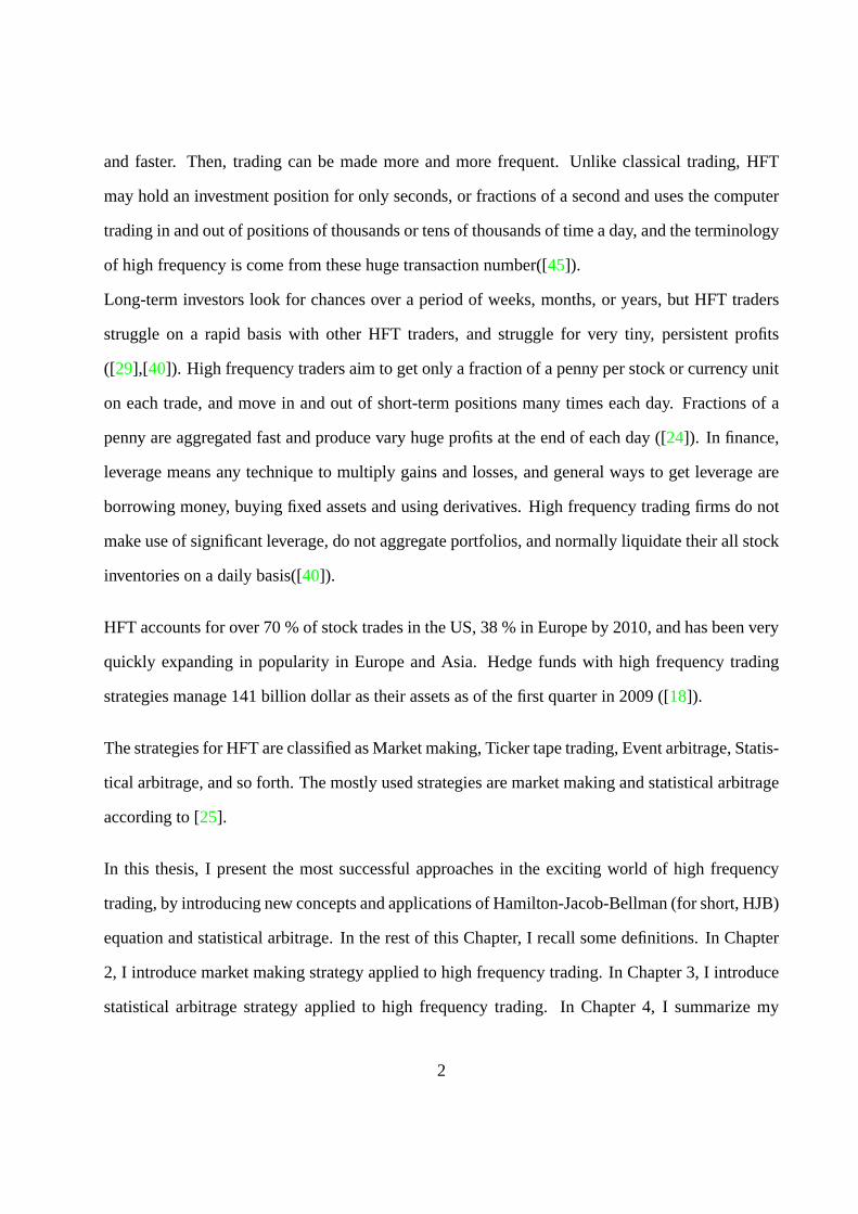
According to [3], HFT has the following three main features : low latency and ultra-low latency
Direct Market Access, multiple asset classes and exchanges, limited shelf life. Classical trading
has a relatively high latency, no Direct Market Access, simple asset classes and exchanges, longer
shelf life. Figure 1.1 shows the comparison between HFT, algorithm trading (AT), and traditional
trading. We now make a little explanation.
6
Figure 1.1: Traditional vs HFT
Low Latency, Ultra-Low Latency Direct Market Access(ULLDMA)
HFT strategies depend on ultra-low latency, which means that the reaction speed is very fast, and
it is illustrated in figure 1.1. HFT trader has to have a real-time, co-located, HFT program which
data is aggregated, and orders are made, directed and implemented in sub-millisecond times, to
figure out any real benefit by executing these strategies.
Direct Market Access (DMA) and Direct Strategy Access (DSA) are the electronic trading facilities
that give HFT investors wishing to trade in financial instruments a way to interact with the order
book of an exchange and are the high speed trading systems to connect directly between trading
desk and stock exchange (like NYSE, NASDAQ). They are means to implement trading flow on
7
a selected place by going around the brokers elective methods. In HFT the DMA should not
postpone orders by more than a millisecond.
At the time of writing, market contacts suggest that some HFT participants in FX can operate with
latency of less than one millisecond, compared with10− 30 milliseconds for most upper-tier non-
HFT participants (for comparison, it is said to take around 150 milliseconds (= 320
seconds) for a
human being to blink).
Multiple asset classes and exchanges
The suitable framework is required to use long connectivity between different data places because
HFT strategies handle transactions in multiple asset classes and across multiple exchanges.
Limited shelf life or Short holding position period
Over time the competitive advantage of HFT strategies decrease. Thus a firm’s micro-level strate-
gies are constantly changed for two reasons even though its high level trading strategy continue
persistently over time. First, HFT traders should constantly change the code to reflect tiny modi-
fication in the progressive market since HFT is dependent on very precise market interactions and
stock correlations. Secondly, competitive intelligence is so smart across rival trading firms that
each is exposed to the increasing susceptibility of their strategies being mimic, turning their most
profitable ideas into their most risky.
8
The advantages of HFT
In [2], the authors demonstrate the following advantages of HFT. Supporters of HFT insists the
following positive points. They are the contraction of the bid-ask spread, the increase in the speed
of execution, improvement in liquidity on platforms, the cushioning of volatility, reduction in
trading fees, and a general increase in the efficiency of the market.
Bid-ask spread
HFT traders can swiftly control the bid and ask prices to provide to new market system through
the fast speed of their system. Thus, without increase of their volatility they can keep their price
close to a certain standard price. The faster speed, the smaller bid-ask spread, and it causes lower
trading costs for market participants and more attractive system.
Liquidity
Numerous limit orders in LOB mean liquidity and HFT brings enormous liquidity in inside market.
The bid-ask spread and the depth of LOB, the number of stocks for limit orders in LOB, are
frequently referred as an indicator of liquidity.
Speed
High speed represents less time for negative price changes between placing and executing the order.
In classical trading, an adverse selection problem was big problem, and it is that ‘late investor’ can
do transaction against the ‘earlier investor’ because ‘late investor’ can have new information when
they are waiting and have a price advantage. However, HFT brings less adverse selection problem
9

through extremely high speed.
Volatility
HFT can continue to set price even in volatile periods, and it means that HFT guarantee liquidity
and more stable price. The fourth quarter of 2008 is a good example.
Increased market efficiency
Market making by HFT is a kind of arbitrage, what the market deletes abnormal prices. Therefore,
it brings increased market efficiency.
Fee
As described above, the faster speed in HFT caused the smaller bid-ask spread and it decreased the
transaction costs for market participants.
10
CHAPTER 2: INTRODUCTION OF MARKET MAKING
Previously, specialist firms implemented the role of market maker. However, nowadays large num-
ber of HFT investors implement HFT strategy due to Direct Market Access (DMA). The reduced
market spreads and the reduced indirect costs for final investors are caused by improved competi-
tion among liquidity providers.
The study shows that the new market provides ideal conditions for HFT market-making, low fees
(i.e., rebates for quotes that led to execution) and a fast system, yet the HFT was equally active
in the official market to remove nonzero positions. A significant improvement in liquidity supply
was further brought by new market entry and HFT. The order driven markets organized most of
modern stock exchanges, and in this kind markets, by posting either market orders or limit orders,
any market participant can participate to with Limit Order Book (LOB).
Features of market making strategies
Typical features of market making strategies are the following. First, market making does not
benefit from stock price going up or down and so is not directional. Second, market makers do
not want to hold any risky asset at the end of the trading day, which means that they do not keep
overnight position. Third, during the trading day, market maker’s positions on the risky asset (i.e.,
stock) are close to zero, and they often balance equally their positions on several different market
by using high frequency order.
At [22] in 1981, Ho and Stoll studied the optimal dealer problem and applied HJB equation to
the market making strategy. In [4], a structure is introduced to control inventory risk in a typical
LOB, and in the context of limit orders trials happening at jump times of Poisson processes, market
11

maker’s goal is maximizing the expected utility of her final profit. This model, called as inventory-
based strategy, shows its efficiency to reduce inventory risk, measured via the variance of terminal
wealth, against the symmetric strategy. This model based on HJB equation introduced by Ho and
Stoll is the first one applied to HFT and is often referred in real world with the LOB model from
[4].
In [19], the authors derived a simplified solution to the backward optimization problem, an in-
depth discussion of its characteristics and an application to the liquidation problem. [6] provided
a closely relevant model to solve a liquidation problem, and study continuous limit case.
In [10] the authors give us a method to include more exact empirical characteristics to this system
by embedding a hidden Markov model for high frequency dynamics of LOB. [32] solve the Mer-
ton’s portfolio optimization problem in the situation where the investor is able to select between
market orders or limit orders. [44] said that in the context of market making in the foreign ex-
change market, it is possible to use market orders in addition to limit orders. In 2011, [20] presents
a novel approach to the issue of optimal high frequency trading with limit and market order. In this
paper they develop a new model to address three sources of risk : the inventory risk, the adverse
selection risk, and the execution risk.
In this thesis, by choosing optimally between market and limit orders from her transactions in the
LOB, and controlling the inventory, and getting rid of her inventory at the terminal date, we, as
a HFT trader, maximize the expected utility function from profit over a finite time horizon T. We
study in detail classical frameworks including power utility criterion and log utility criterion.
Market-making Model
We now recall some definitions.
12
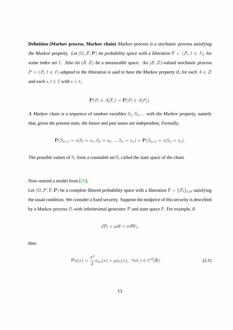
Definition (Markov process, Markov chain) Markov process is a stochastic process satisfying
the Markov property. Let(Ω,F ,P) be probability space with a filterationF = (Ft, t ∈ I), for
some index setI. Also let (S,Z) be a measurable space. An(S,Z)-valued stochastic process
P = (Pt, t ∈ I) adapted to the filteration is said to have the Markov property if, for eachA ∈ Z
and eachs, t ∈ I with s < t,
P(Pt ∈ A|Fs) = P(Pt ∈ A|Ps).
A Markov chain is a sequence of random variablesS1, S2, ... with the Markov property, namely
that, given the present state, the future and past states are independent, Formally,
P(Sn+1 = s|S1 = s1, S2 = s2, ..., Sn = sn) = P(Sn=1 = s|Sn = sn).
The possible values ofSi form a countable setS, called the state space of the chain.
Now remind a model from [20].
Let (Ω,F ,F,P) be a complete filtered probability space with a filterationF = {Ft}t≥0 satisfying
the usual condition. We consider a fixed security. Suppose the midprice of this security is described
by a Markov processPt with infinitesimal generatorP and state spaceP. For example, if
dPt = μdt + σdWt,
then
Pφ(x) =σ2
2φxx(x) + μφx(x), ∀φ(∙) ∈ C2(R). (2.1)
13

To describe the spread process, letSn be a discrete-time stationary Markov chain taking values in
the finite state space
S ≡ {iδ∣∣ 1 ≤ i ≤ m},
whereδ > 0 is a fixed constant called the tick size, andm > 1 is a given (possibly large) in-
teger (see table 2.3 on page 21). Let the probability transition matrix ofSn be given byR0 =
(ρij)1≤i,j≤m, i.e.,
P (Sn+1 = jδ|Sn = iδ) = ρij (2.2)
andρii = 0.
Next, letNt be a Poisson process with a deterministic intensity rateλ(t), which is independent of
Sn. Then, the price spread process is assumed to be
St = SNt , t ≥ 0, (2.3)
whereNt = (Nat , N b
t ), with N bt being the number of arrivals of market bid orders matching the
limit orders for quote askQa, andNat being the number of arrivals of market ask orders matching
the limit orders for quote bidQb.
Also, we assume thatSt is independent of the Poisson processN . Thus,St is a continuous-time
Markov chain taking values inS, with intensity matrixR(t) = λ(t)R0, whereλ(t) is a parameter of
Poisson distribution and it is the numbers which market order hits limit order, which is the number
of trading execution.
For a HFT trader, she can trade the stock by either limit orders or market orders. More precisely,
14

she may post at any time limit bid/ask orders at the current best bid/ask prices, and then has to wait
an incoming counterpart market order engaging her limit order. She can also post market bid/ask
orders to execute immediately, but, in this case obtain the opposite best quote, i.e. trades at the
best-ask/best-bid price, which is less beneficial.
Figure 2.1: Example of Limit Order Book [35]
Limit Order strategy
At any time the HFT trader may post limit bid/ask orders indicating the quantity and the price
she want to pay/receive per stock (called limit price), and trade will be completed only when an
incoming market ask/bid order ‘hits’ matching her limit bid/ask order. The HFT trader quotes the
bid priceQbt with quantityLb
t and the ask priceQat with quantityLa
t , and she is committed to re-
spectively buy and sell the stock at these prices. In other words, these limit orders will be traded
when a market order comes with promised quantitiesLbt or La
t (see figure 2.2).
15

Figure 2.2: Schematic of a LOB
In stock market, consecutive event such as order flow has strong relationship with Poisson distri-
bution and Exponential distribution in statistics. Because the events in LOB happens in very short
time, in very complicated, and almost consecutively, we have to analyze them statistically. Poisson
distribution focuses on how many times the events happen per unit time, while exponential distri-
bution focuses on how long the event takes time per each event. Let us look at a concrete case to
get some feeling.
Assume that a spread iss %, which is a constant. Figure 2.2 illustrates the definitions in this part
and represents a schematic of LOB at some instant in time. By the definition of spread observed
prices for buys, the bid prices, are lower than the actual midprices by0.5s %, but observed prices
for sells, the ask prices, are higher than the actual price by0.5s % (see equation (2.4)). If we
assume that the daily high price is a buyer-initiated trade, so it is grossed up by half of the spread,
16

but the daily low price is a seller-initiated trade, so it is discounted by half of the spread. Therefore
the observed high-low price range includes both the range of the actual prices and the bid-ask
spread.
We assume that the arrival market bid orders which will trade our trader’s limit ask orders follow
a Poisson process with an intensity rateλa(qat , st), wherest is the spread,qa
t is an ask quote.
Likewise, the arrival market ask orders which will hit the trader’s limit bid orders follow a Poisson
process with an intensity rateλb(qbt , st), whereqb
t is a bid quote.
Suppose thatpbt andpa
t are current best bid price and current best ask price respectively, andδbt
should be an integer multiple of the so-called tick sizesδ for bid, δat should be an integer multiple
of the so-called tick sizesδ for ask, the smallest increment (tick) by which the price of stocks can
move.
HFT trader try to defeat with the other trader, and it means that the trader could post limit ask order
at pat or pa
t − δ, the improved ask price, and post limit bid order atpbt or pb
t + δ, the improved bid
price, to sell/buy as soon as possible. LetYt be the stock inventory process andXt be the cash
process at timet. If a bid limit order is made att, we denote the limit bid price byQbt and limit
bid order size byLbt . Thus,(Qb
t , Lbt) determines a limit bid order. Likewise, we may let(Qa
t , Lat )
represent a limit ask order. We restrictQbt andQa
t to be the following form:(see figure 2.2, table
2.1, table 2.3)
Qbt = Pt− −
Sbt−
2+ δb
t = P bt− + δb
t ,
Qat = Pt− +
Sat−
2− δa
t = P at− − δa
t , (2.4)
with
δbt , δa
t ∈ {0, δ},
17
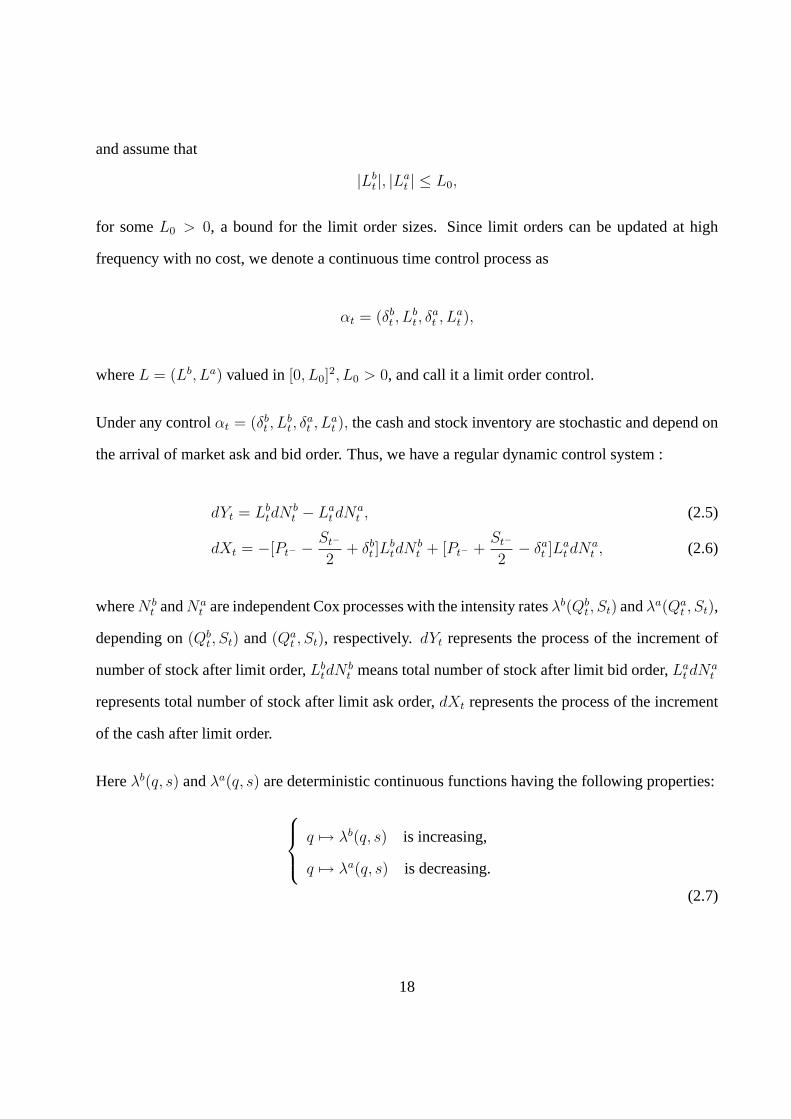
and assume that
|Lbt |, |L
at | ≤ L0,
for someL0 > 0, a bound for the limit order sizes. Since limit orders can be updated at high
frequency with no cost, we denote a continuous time control process as
αt = (δbt , L
bt , δ
at , L
at ),
whereL = (Lb, La) valued in[0, L0]2, L0 > 0, and call it a limit order control.
Under any controlαt = (δbt , L
bt , δ
at , L
at ), the cash and stock inventory are stochastic and depend on
the arrival of market ask and bid order. Thus, we have a regular dynamic control system :
dYt = LbtdN b
t − Lat dNa
t , (2.5)
dXt = −[Pt− −St−
2+ δb
t ]LbtdN b
t + [Pt− +St−
2− δa
t ]Lat dNa
t , (2.6)
whereN bt andNa
t are independent Cox processes with the intensity ratesλb(Qbt , St) andλa(Qa
t , St),
depending on(Qbt , St) and(Qa
t , St), respectively.dYt represents the process of the increment of
number of stock after limit order,LbtdN b
t means total number of stock after limit bid order,Lat dNa
t
represents total number of stock after limit ask order,dXt represents the process of the increment
of the cash after limit order.
Hereλb(q, s) andλa(q, s) are deterministic continuous functions having the following properties:
q 7→ λb(q, s) is increasing,
q 7→ λa(q, s) is decreasing.
(2.7)
18

We letA[t, T ] be the set of all limit order controls on[t, T ].
In Table 2.1, let us consider a simple LOB having five limit orders, namely, sell 150 shares stock
of SAMSUNG at $10.11, sell 150 shares stocks of SAMSUNG at $10.08, buy 100 shares stocks
of SAMSUNG at $10.05, buy 200 shares stocks of SAMSUNG at $10.01.
Table 2.1: Before two market orders
Price Ask Size$10.11 150$10.08 100
300 $10.05200 $10.01
bid Size Price
Orders to buy/sell are orders on the bid/ask side. The prices are $10.11, $10.08, $10.05, $10.01.
$10.05 is the highest bid price and it is called the best bid, and $10.08 is the lowest ask price and
it is named the best ask, and they consist of the inside market. The difference between the best bid
and best ask is called the spread (= $10.08-$10.05 = $0.03). The average of the best bid and best
ask is called the midprice ($10.08+$10.652
= $10.065).
HFT traders can submit four kinds of messages to an LOB, and they are add, cancel, cancel/replace,
and market order. A trader can add and cancel(remove) a limit order in to the LOB. Suppose a
trader needs to reduce the size of her order, then she can submit a cancel/replace. So the current
order will be canceled and be replaced with the order with a lower size at the same price.
Let us start to have two market orders. First, every orders have ‘timestamps’ representing the time
accepted into the LOB, and they bring the time priority of an order. In other words, before later
orders earlier orders will be traded. For example, in Table 1 let us assume that the order buying 200
stocks at $10.05 was submitted after the order buying 100 stocks at $10.05, and then LOB has 300
19

bid size for $10.05. Assume that a HFT trader submit a market bid order to sell total 200 stocks
to LOB. Then 100 shares of the order with 200 total shares will be traded after the limit order for
100 stocks is executed because the earlier 100 stocks was the first in the queue and 100 shares of
the order with 200 total shares was the second in the queue. After this market order of 200 shares,
100 stocks will stay in the LOB at price $10.05.
Second, if a market order has more stocks than the size at the inside market, it will trade at worse
price until it end. For example, if a HFT trader submit a market order buying 200 stocks, then the
order at $10.08 would be completely traded because $10.08 is the best ask price currently. Next
100 stocks of $10.11 will be executed to finish the market order. An order to sell 50 stocks at the
price level of $10.11 will be in the LOB. The following LOB is the one after we executed above
two market orders.
Table 2.2: After two market orders
Price Ask Size$10.11 50
100 $10.05200 $10.01
bid Size Price
Now we consider more complicated LOB, and assume that all tick sizes are same in Table 2.3. Let
us consider the LOB of table 2.3. In the left table, spread = best ask (pa) - best bid (pb) = $150 -
$130 = $20, and mid-price =pa+pb
2= $150+$130
2= $140. Tick sizeδ = increment = $10. If a HFT
trader submit limit bid order by $130 an limit ask order by $150, and these contracts happen, then
$150 - $130 = $20 would be the profits (= spread). If a HFT trader submit limit bid order by $120
an limit ask order by $160, and these trades happen, then $160 - $120 = $40 would be the profits
(= spread + 2δ). In the right table, equation (1) - equation (3) = bid-ask spreads by definition.
20

Table 2.3: Example of LOB
$180 p + S2
+ 3δ pa + 3δ$170 p + S
2+ 2δ pa + 2δ
$160 p + S2
+ δ pa + δ$150 Best Ask p + S
2(1) pa=possibleqa
$140 Mid-price p (2) pa − δ=possibleqa(4), pb + δ = possibleqb(5)$130 Best Bid p − S
2(3) pb=possibleqb
$120 p − S2− δ pb − δ
$110 p − S2− 2δ pb − 2δ
$100 p − S2− 3δ pb − 3δ
If limit ask order occur bypa − δ and limit bid order happen bypb, equation (4) - equation (3) =
s − δ = HFT trader’s profit.
Market order strategies
The HFT trader may submit market orders to have an immediate execution reducing his inventory.
Unlike limit orders, market order (strategy) takes liquidity in the market because market orders
take incoming limit orders, and have fees.
Also, a market order strategy can be described by an impulse control, calledβ. More precisely,
we may let{τn}n≥1 be an increasing sequence ofF-stopping times, representing the moments at
which market orders are posted, and for eachn ≥ 1, {ζn}n≥1 is a sequence ofFτn-measurable
random variables valued in[−z, z], z > 0, representing the amount traded at the moments. While
submitting a market orderζn at τn, the cash and stock inventory jump dynamic control system at
time τn as follows.
Yτn = Yτ−n
+ ζn, (2.8)
Xτn = Xτ−n− c(ζn, Pτ−
n, Sτ−
n), (2.9)
21
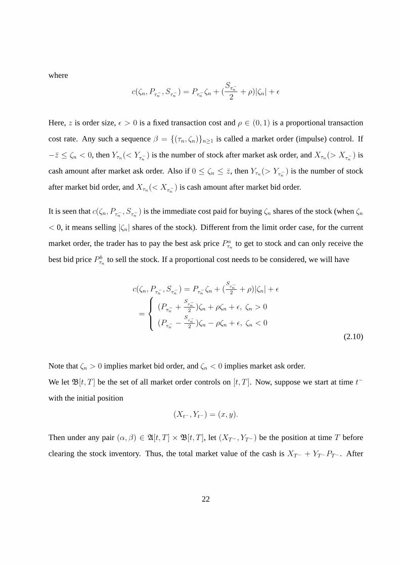
where
c(ζn, Pτ−n, Sτ−
n) = Pτ−
nζn + (
Sτ−n
2+ ρ)|ζn| + ε
Here,z is order size,ε > 0 is a fixed transaction cost andρ ∈ (0, 1) is a proportional transaction
cost rate. Any such a sequenceβ = {(τn, ζn)}n≥1 is called a market order (impulse) control. If
−z ≤ ζn < 0, thenYτn(< Yτ−n) is the number of stock after market ask order, andXτn(> Xτ−
n) is
cash amount after market ask order. Also if0 ≤ ζn ≤ z, thenYτn(> Yτ−n) is the number of stock
after market bid order, andXτn(< Xτ−n) is cash amount after market bid order.
It is seen thatc(ζn, Pτ−n, Sτ−
n) is the immediate cost paid for buyingζn shares of the stock (whenζn
< 0, it means selling|ζn| shares of the stock). Different from the limit order case, for the current
market order, the trader has to pay the best ask priceP aτn
to get to stock and can only receive the
best bid priceP bτn
to sell the stock. If a proportional cost needs to be considered, we will have
c(ζn, Pτ−n, Sτ−
n) = Pτ−
nζn + (
Sτ−n2
+ ρ)|ζn| + ε
=
(Pτ−n
+S
τ−n2
)ζn + ρζn + ε, ζn > 0
(Pτ−n−
Sτ−n2
)ζn − ρζn + ε, ζn < 0
(2.10)
Note thatζn > 0 implies market bid order, andζn < 0 implies market ask order.
We letB[t, T ] be the set of all market order controls on[t, T ]. Now, suppose we start at timet−
with the initial position
(Xt− , Yt−) = (x, y).
Then under any pair(α, β) ∈ A[t, T ] ×B[t, T ], let (XT− , YT−) be the position at timeT before
clearing the stock inventory. Thus, the total market value of the cash isXT− + YT−PT− . After
22

clearing the stock inventory, the cash becomes
XT = XT− + YT−PT− − |YT− |(ST−
2+ ρ)− ε. (2.11)
Optimal control problem
The goal of the HFT trader is to maximize the expected utility from revenue over a finite time
horizonT , by choosing optimally limit and market orders.
We now introduce the following payoff objective functional:
J(t, x, y, p, s; α, β) = E[U(XT ) −
∫ T
t
g(Yt)dt], (2.12)
whereU(∙) is a utility function, a level of satisfaction, andg(Yt) : R → (0,∞) is a continuous
penalty function. The second term on the right hand side of the equation (2.12) represents a penalty
on the stock inventory, and we can select it arbitrarily. Our optimal control problem can be stated
as follows.
Problem (C). ∀(t, x, y, p, s) ∈ [0, T ) × R× R× P× S, find a pair(α, β) ∈ A[t, T ] ×B[t, T ]
such that
J(t, x, y, p, s; α, β) = sup(α,β)∈A[t,T ]×B[t,T ]
J(t, x, y, p, s; α, β) ≡ V (t, x, y, p, s), (2.13)
where(α, β) is limit and market order trading strategies, respectively. The functionV (t, x, y, p, s)
is called the value function of Problem (C), and problem (C) is a mixed regular and impulse control
problem in a regime switching jump-diffusion model.
23

Dynamic programming equation (DPE)
The dynamic programming principle (DPP) is a fundamental principle in optimal stochastic control
theory. It gives a relationship among dynamic control systems, problem (C), via value function.
For the above problem (C), we have the following dynamic programming principle.
Theorem. For any(t, x, y, p, s) ∈ [0, T ) × R× R× P× S,
V (t, x, y, p, s) ≥ supz∈R
V(t, x − c(z, p, s), y + z, p, s
)≡M[V ](t, x, y, p, s), (2.14)
and
V (t, x, y, p, s) ≥ supα∈A[t,T ]
E[V (t, Xt, Yt, Pt, St)
], ∀t ∈ (t, T ]. (2.15)
If the strict inequality holds in the(2.14), then there exists aσ > 0 such that
V (t, x, y, p, s) = supα∈A[t,T ]
E[V (t, Xt, Yt, Pt, St)
], ∀t ∈ [t, t + σ]. (2.16)
Note thatV (t, x, y, p, s) is all kind of possible strategies, andV(t, x− c(z, p, s), y + z, p, s
)is one
market order strategy , andV (t, Xt, Yt, Pt, St) is one limit order strategy.
From the above. we have
24
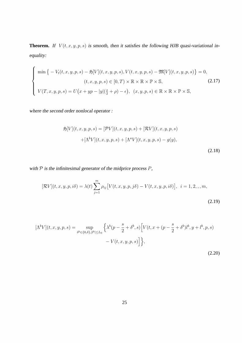
Theorem. If V (t, x, y, p, s) is smooth, then it satisfies the following HJB quasi-variational in-
equality:
min{− Vt(t, x, y, p, s) − H[V ](t, x, y, p, s), V (t, x, y, p, s) −M[V ](t, x, y, p, s)
}= 0,
(t, x, y, p, s) ∈ [0, T ) × R× R× P× S,
V (T, x, y, p, s) = U(x + yp − |y|( s
2+ ρ) − ε
), (x, y, p, s) ∈ R× R× P× S,
(2.17)
where the second order nonlocal operator :
H[V ](t, x, y, p, s) = [PV ](t, x, y, p, s) + [RV ](t, x, y, p, s)
+[ΛbV ](t, x, y, p, s) + [ΛaV ](t, x, y, p, s) − g(y),
(2.18)
with P is the infinitesimal generator of the midprice processP ,
[RV ](t, x, y, p, iδ) = λ(t)m∑
j=1
ρij
[V (t, x, y, p, jδ) − V (t, x, y, p, iδ)
], i = 1, 2, , ,m,
(2.19)
[ΛbV ](t, x, y, p, s) = supδb∈{0,δ},|lb|≤L0
{λb(p −
s
2+ δb, s)
[V (t, x + (p −
s
2+ δb)lb, y + lb, p, s)
− V (t, x, y, p, s)]}
,
(2.20)
25
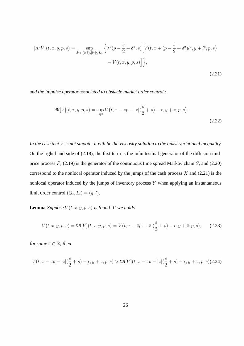
[ΛaV ](t, x, y, p, s) = supδa∈{0,δ},|la|≤L0
{λa(p −
s
2+ δa, s)
[V (t, x + (p −
s
2+ δa)la, y + la, p, s
)
− V (t, x, y, p, s)]}
,
(2.21)
and the impulse operator associated to obstacle market order control :
M[V ](t, x, y, p, s) = supz∈R
V(t, x − zp − |z|(
s
2+ ρ) − ε, y + z, p, s
).
(2.22)
In the case thatV is not smooth, it will be the viscosity solution to the quasi-variational inequality.
On the right hand side of (2.18), the first term is the infinitesimal generator of the diffusion mid-
price processP , (2.19) is the generator of the continuous time spread Markov chainS, and (2.20)
correspond to the nonlocal operator induced by the jumps of the cash processX and (2.21) is the
nonlocal operator induced by the jumps of inventory processY when applying an instantaneous
limit order control(Qt, Lt) = (q, l).
Lemma SupposeV (t, x, y, p, s) is found. If we holds
V (t, x, y, p, s) =M[V ](t, x, y, p, s) = V (t, x − zp − |z|(s
2+ ρ) − ε, y + z, p, s), (2.23)
for somez ∈ R, then
V (t, x − zp − |z|(s
2+ ρ) − ε, y + z, p, s) >M[V ](t, x − zp − |z|(
s
2+ ρ) − ε, y + z, p, s).(2.24)
26
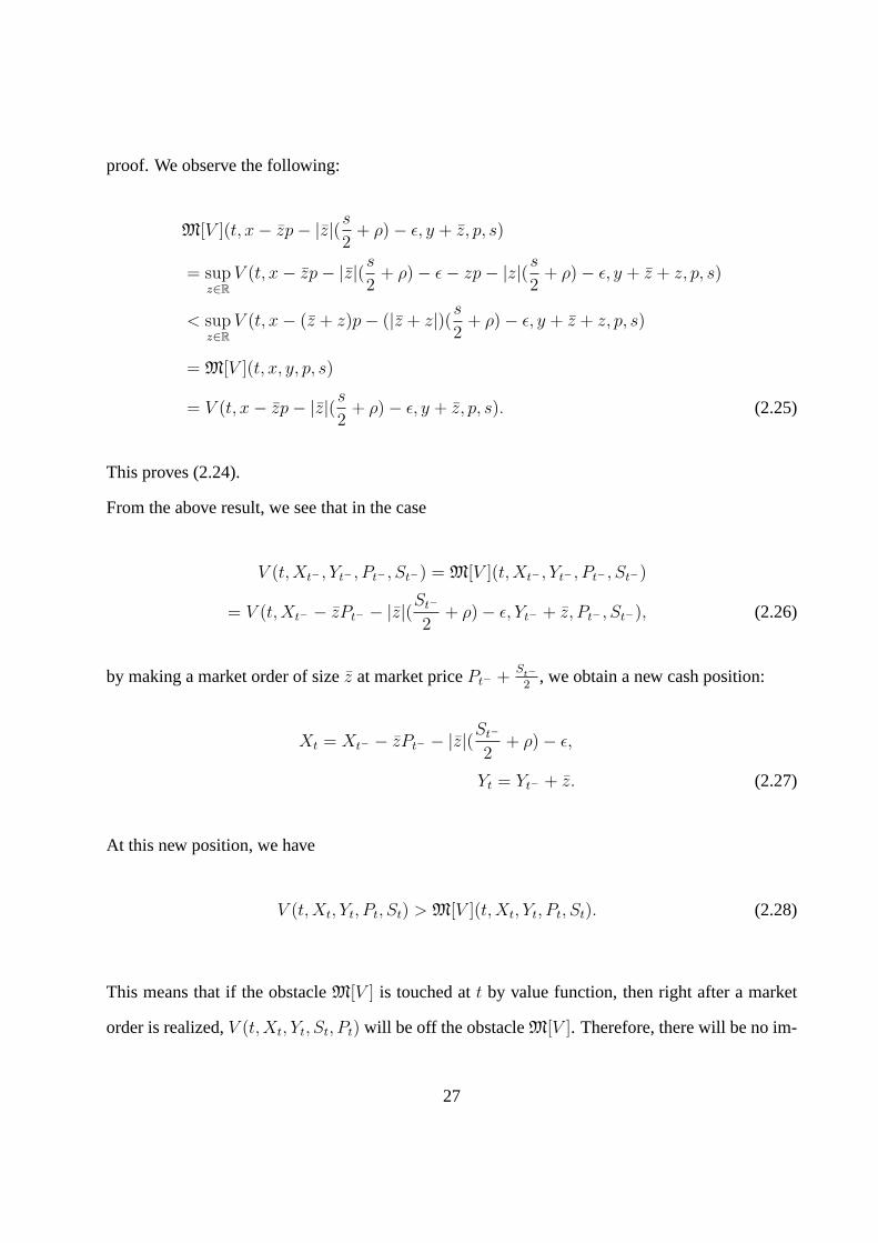
proof. We observe the following:
M[V ](t, x − zp − |z|(s
2+ ρ) − ε, y + z, p, s)
= supz∈R
V (t, x − zp − |z|(s
2+ ρ) − ε − zp − |z|(
s
2+ ρ) − ε, y + z + z, p, s)
< supz∈R
V (t, x − (z + z)p − (|z + z|)(s
2+ ρ) − ε, y + z + z, p, s)
=M[V ](t, x, y, p, s)
= V (t, x − zp − |z|(s
2+ ρ) − ε, y + z, p, s). (2.25)
This proves (2.24).
From the above result, we see that in the case
V (t,Xt− , Yt− , Pt− , St−) =M[V ](t,Xt− , Yt− , Pt− , St−)
= V (t,Xt− − zPt− − |z|(St−
2+ ρ) − ε, Yt− + z, Pt− , St−), (2.26)
by making a market order of sizez at market pricePt− +St−
2, we obtain a new cash position:
Xt = Xt− − zPt− − |z|(St−
2+ ρ) − ε,
Yt = Yt− + z. (2.27)
At this new position, we have
V (t,Xt, Yt, Pt, St) >M[V ](t,Xt, Yt, Pt, St). (2.28)
This means that if the obstacleM[V ] is touched att by value function, then right after a market
order is realized,V (t,Xt, Yt, St, Pt) will be off the obstacleM[V ]. Therefore, there will be no im-
27
mediate market order right after. Hence, right after, we may assume that the above strict inequality
holds fort ∈ (τ1, τ2). Then the trader will not make market orders during this time period. Let us
look how she will make limit orders in the time period.
Suppose we have(δb, lb) and(δa, la) with
δb = δb(t, x, y, p, s), lb = lb(t, x, y, p, s),
δa = δa(t, x, y, p, s), la = la(t, x, y, p, s),
such that
[ΛbV ](t, x, y, p, s) = supδb∈{0,δ},|lb|≤L0
{λb(p −
s
2+ δb, s)
[V (t, x + (p −
s
2+ δb)lb, y + lb, p, s)
− V (t, x, y, p, s)]}
= λb(p − s2
+ δb, s)[V (t, x + (p − s
2+ δb)lb, y + lb, p, s) − V (t, x, y, p, s)
],
[ΛaV ](t, x, y, p, s) = supδa∈{0,δ},|la|≤L0
{λa(p +
s
2− δa, s)
[V (t, x + (p +
s
2− δa)la, y + la, p, s)
− V (t, x, y, p, s)]}
= λa(p + s2− δa, s)
[V (t, x + (p + s
2− δa)la, y + la, p, s) − V (t, x, y, p, s)
]}.
Then during the time period that the obstacleM[V ] is not touched, the investor can set up two limit
orders:
28

Qbt = Pt− −
Sbt−
2+ δb
t−(t,Xt, Yt, Pt, St) = P bt− + δb
t−(t,Xt, Yt, Pt, St),
Lbt = lb(t,Xt, Yt, Pt, St),
Qat = Pt− +
Sat−
2− δa
t−(t,Xt, Yt, Pt, St) = P at− − δa
t−(t,Xt, Yt, Pt, St),
Lat = la(t,Xt, Yt, Pt, St).
This will lead to an optimal policy on the time interval in which the obstacle is not touched. Com-
bining the above, we have the following result.
Theorem. The value functionV (t, x, y, p, s) is the unique viscosity solution to the quasi-variational
inequality(2.17)and through which an optimal trading strategy can be constructed.
29
CHAPTER 3: STATISTICAL ARBITRAGE
Definition
Statistical arbitrage is to use predictable temporary deviations from stable statistical relationships
among stocks, and it is actively used in all liquid stocks, stocks that is easily sold due to the fact that
there is a large volume of shares traded every day, like equities, bonds, futures, foreign exchange,
etc. Classical arbitrage may also be involved with such strategy. One example of classical arbitrage
is the covered interest rate parity, a no-arbitrage condition representing an equilibrium state under
which investors will be indifferent to interest rates available on bank deposits in two countries,
in the foreign exchange market. It gives a connection between the prices of a domestic bond, a
bond denominated in a foreign currency, the spot price of the currency, and the price of a forward
contract on the currency.
Statistical arbitrage used for HFT uses very complicated models containing many more than four
stocks. The TABB Group obtains now annual total profits overUS$21 billion by this strategy.
Pairs trading
To exploit the long-term statistical relationships that often exist between assets statistical arbitrage
trading strategies are commonly applied in industry. The most well-known application in finance is
an investment strategy known as ‘pairs trading’, and it is the simplest form of statistical arbitrage.
It is a market neutral trading strategy who makes HFT traders to earn returns from any market
conditions: uptrend, downtrend, or sideways movement, (neither an uptrend nor a downtrend).
Also it is classified as a statistical arbitrage and convergence trading strategy.
30
Gerry Bamberger developed this pairs trading and Nunzio Tartaglias quantitative group at Morgan
Stanley applied more to market in the 1980s. Pairs trading compares the results of two historically
correlated stocks. When the two stocks correlated weakly, i.e. one stock going up when the other
going down, the strategy of pairs trading will be to short (= sell) the outperforming security and to
long (= buy) the underperforming one, expecting the convergence of the spread between the two
stocks in the future.
When there are temporary supply (or demand) changes, large buy (or sell) orders for one security,
reaction for important news about one of the companies, and so on, the divergence within a pair
occurs.
The opportunity is rare even though pairs trading strategy does not have much downside risk, an
estimation of a security’s potential to suffer a decline in value if the market conditions change, or
the amount of loss that could be sustained as a result of the decline. So the HFT trader should be
one of the first to gain a profit. It is hard to anticipate individual stock prices but it might be easy
to anticipate the price (or the spread series) of certain stock portfolio. To anticipate the price (or
the spread series) of certain stock portfolio, the first step is establishing the portfolio so that the
spread series is a stationary process, a stochastic process whose joint probability distribution does
not change when shifted in time or space. As the second step, the stationary process is achieved by
finding a cointegration relationship, a statistical property of time series variables, between the two
stock price series. We say that two or more time series are cointegrated if they share a common
stochastic drift. As long as the spread series is a stationary processes no matter how portfolio is
established, then it can be modeled, and subsequently anticipated, using techniques of time series
analysis such as Ornstein-Uhlenbeck models, autoregressive moving average (ARMA) models and
(vector) error correction models.
HFT traders consider forecastability of the portfolio spread series to be important by the following
31
reasons : First, by buying and selling the shares the spread can be directly traded. Second, The
return and risk of the trade can be measured by the forecast and its error bounds given by the
model.
Financial engineers has been interested in figure out the outcome of statistical arbitrage for two rea-
sons. First, [14] said that in the debate over whether financial markets are efficient, such strategies
violate the weakest form of market efficiency. Second, the market frictions (anything preventing
markets from developing and working properly) or behavioral biases cause prices to deviate from
fundamental values, and statistical arbitrage make financial engineers to understand it ([23])
Now many researchers have studied to understand the source of profitability in these strategies
because there are many papers about the profitability of these strategies. [16] said that the un-
expected change of trading volume also captures informational effects due to increased visibility
of the equities, the profits from pairs trading may be negatively affected by the change of trading
volume.
A paper said that a pairs trading strategy generates annual returns of 11 percent and a monthly
Sharpe ratio of four to six times more than that of market returns between 1962 and 2002 ([17]).
In 2007, [42] compares the efficacy of the Relative Strength Index (RSI) versus the Moving Av-
erage (MA) trading rules on the daily exchange rates of six currencies. The results indicate that
the trading rules can yield positive risk-adjusted returns, and the profitability of these trading rules
is positively related to central bank interventions. It is also found that the impact of interest rate
differentials on the trading rule return is not important.
32

Moving Average (MA)
Definition
MA(N)t =1
N
N−1∑
i=0
Pt−i, (3.1)
whereN is the length of the moving average, andPt is the stock price at timet.
The MA method is defined as the Simple Moving Average (SMA), which is the unweighted mean
of the previous N data points.
Trading strategy:
a) Long stock ifPt ≥ MA(N)t
b) Short stock ifPt < MA(N)t
If the stock price is above or equal to the MA, then the trading should long (buy) the US dollar,
and if the stock price is below the MA, then the trading is going to short (sell) it.
There are several advantages for MA. First, they smooth out fluctuations in data and show the
trend. Second, time horizon of the trend, a fixed point of time in the future at which point certain
processes will be evaluated or assumed to end, is determined by the period of the MA. Third, it
can be used to generate buy and sell signals using the crossover of several averages. Fourth, it can
save trader from fake-outs. Fifth, SMAs work well for longer-term situations that do not require a
lot of sensitivity.
Disadvantages of MA are the followings. First, because they average the data, they lag the turns
33

in the underlying data. Second, reducing the period of the average reduces the lag but increases
whipsaws, a condition where a security’s price heads in one direction, but then is followed quickly
by a movement in the opposite direction (i.e., false signals). Third, SMA provides a smoother
slope and responds slower to price actions.
Exponential Moving Average (EMA)
EMA is a type of infinite impulse response filter, a filter with a property of signal processing sys-
tems who have an impulse response function that is non-zero over an infinite length of time, that
applies weighting factors which decrease exponentially.
Definition :
EMA(N)t = αPt + (1 − α)EMA(N)t−1, (3.2)
where the coefficientα is the degree of weight decreases, andα = 2N+1
with 0 < α < 1. A higher
α discounts older observations faster.
We need to define the value ofEMA(N)0, the first value of the EMA. The choice ofEMA(N)0 is
not unique. To calculateEMA(N)0 some professionals may use the asset price at the time when
they first implement the strategy, and some may use a SMA of the prior N data points.
Trading Strategy:
a) Long stock ifPt ≥ EMA(N)t
34

b) Short stock ifPt < EMA(N)t.
If the stock price is above or equal to the EMA, then the trading should long the US dollar, and if
the stock price is below the EMA, then the trading is going to short it.
There are several advantages for EMA. First, the EMA best suits to the trader if the trader want a
MA that will quickly respond to price movements, because EMA tends to catch trends very early
and it would yield higher profit for a HFT trader. Second, the earlier the trader see a trend, the
longer the trader will be able to take advantage of it. Third, the EMA weighs current prices more
heavily than past prices. Fourth, EMA respond quicker to short-term situations than long term
situation.
Disadvantages of EMA are the followings. First, trader may get superficial readings during consol-
idation periods, periods of the movement of an asset’s price within a well-defined pattern or barrier
of trading levels. Because EMA tends to catch trends quickly, it can be so fast that you may pick
up a trend which could just be a sudden price change. Second, EMA is more prone to whipsaws.
Third, since EMA respond quicker to short-term situations, it may also be prone to giving false
signals.
However, every HFT trader should weigh the pros and the cons of the EMA and decide in which
manner they will be using MA. Nevertheless, MA remain the most popular and is the most effective
technical analysis indicator out on the market today.
Let us compare between MA and EMA. First, SMA work well for longer-term situations that do
not require a lot of sensitivity. Second, the EMA is more sensitive and better for shorter time
periods as it can capture changes quicker.
35
Relative Strength Index (RSI)
Definition :
RSI(N)t = 100 −100
1 + RS,
(3.3)
whereRS = Average(U,t)Average(D,t)
, and Average(U,t) represents the average of N days (usually 250 days) up
prices and Average(D,t) is average of N days down prices.
The RSI ranges from zero to 100. It gives a reading of zero if there are pure downward price
movements, and a reading of 100 if there are pure upward price movements. The threshold value
is the middle point of the oscillator, 50. The RSI computes momentum, the rate of the rise or fall in
price, as the ratio of higher closes (closing price) to lower closes: stocks which have had more or
stronger positive changes have a higher RSI than stocks which have had more or stronger negative
changes. The RSI is measured on a scale from 0 to 100, and is considered overbought when above
70 and oversold when below 30.
Trading strategy:
a) Long the USD ifRSI(N)t ≥ 50
b) Short the USD ifRSI(N)t < 50
There are several advantage for RSI. First, it is very elegant indicator, whose movements are
smooth, and so it can fit into a simple package between 0 and 100. Second, it is not only a testa-
36
ment to its abilities, but it also makes its signals self-fulfilling prophecy, a prediction that causes
itself to become true due to positive feedback between belief and behavior, at times. People who
believe in the importance of the 50-day moving average, for example, closely monitor their stocks
as they approach that average. Third, when used to indicate divergences, it can be quite powerful.
Disadvantages of RSI are the followings. First, it doesn’t take into account how many up days vs.
down days there are in the range, so one single big decline could offset a large number of gain
periods and only one single big increase could offset a large number of loss periods. Second, the
RSI is also notoriously weak in strongly trending markets, a market that is trending in one direction
or another, because it can remain oversold/overbought for a long time during strong trends and so
HFT traders avoid using RSI in strongly trending markets unless trading in the direction of the
trend.
Sharpe Ratio
The Sharpe ratio or Sharpe index or Sharpe measure or reward-to-variability ratio is a measure of
the excess return (or Risk Premium) per unit of risk in an investment asset or a trading strategy,
named after William Forsyth Sharpe (1966). High-frequency traders compete on a basis of speed
with other high-frequency traders, not long-term investors, and compete for very small, consis-
tent profits. As a result, high-frequency trading has been shown to have a potential Sharpe ratio
thousands of times higher than the traditional buy-and-hold strategies.
Since its revision by the original author in 1994, it is defined as:
Definition : Let X ∼ f(x) with E(X) = μ andV ar(X) = σ2,
37
whereX is random variable andf(x) is distribution function. Then, the value
Sharpe =r − rf
σ(3.4)
is called the Sharpe ratio of X, wherer is rate of return,rf is a risk-free (interest) rate, andσ is
standard deviation, which is a risk.
Thus, the higher the Sharpe ratio, the higher the risk-adjusted return.
Example :
Suppose that portfolio A have a 10 % rate of return with a volatility of 0.10. US treasury bills
are frequently considered as the criterion for risk free (interest) rate. Assume average return of
the treasury bills during the 20 th century is about 0.9 %. Then, the sharpe ratio for portfolio A is
0.10−0.0090.10
= 0.91 by equation (3.4). But to evaluate this number we have to have the other sharpe
ratio to compare together.
Now, assume portfolio B has bigger standard deviation,0.15, than portfolio A and the same rate
of return, and same risk free rate. Then by the equation (3.4) sharpe ratio is0.100.0090.15
= 0.15. Thus,
portfolio B have a smaller sharpe ratio than portfolio A. This result is understandable because both
investment have the same return but portfolio B have a bigger risk. In obvious, we prefer the
investment whose risk is less if the given return is same. Suppose two investments have the same
risks and one of two gives us a bigger return. Then obviously we prefer the portfolio with the
bigger return by the most basic principles of investment, and it can be showed by sharpe ratio in
mathematically.
38
Suppose that portfolio C gives the same volitility as portfolio B but has higher return of 20 %.
Then 0.20−0.0090.15
= 1.91 would be sharpe ratio. As a result, the ratio of portfolio C,1.27, is much
higher than the one of portfolio B,0.61.
It gets a bit more complicating when portfolio A is compared to portfolio C. Portfolio A has a
lower rate of return, but it is also very low risk. Portfolio C offers higher returns for higher risk.
Simply glancing at the details of the two portfolios is not enough to determine which one is a better
investment. This is where the Sharpe ratio comes into play. Portfolio A has a ratio of 0.91 and
portfolio C has a ratio of 1.27, indicating that the risk of portfolio C is well worth the returns as
compared to A.
When comparing two portfolios with the same risk or return, it is easy to see which one is a better
choice. However, when looking at two options with completely different details it can be hard to
determine which one provides the better return for risk. By plugging the numbers into the simple
equation known as the Sharpe ratio, the return versus risk factor can easily be determined.
The Sharpe ratio is used to characterize how well the return of an asset compensates the HFT
investor for the risk taken, and therefore the higher the Sharpe ratio number the better. When
comparing two assets each with the expected return against the same benchmark with return , the
asset with the higher Sharpe ratio gives more return for the same risk.
HFT investors are often advised to pick investments with high Sharpe ratios. However like any
mathematical model it relies on the data being correct. When examining the investment perfor-
mance of assets with smoothing (standardization) of returns, the Sharpe ratio should be derived
from the performance of the underlying assets rather than the fund returns. Some Sharpe ratios are
often used to rank the performance of portfolio or mutual fund managers.
39

But we should note that if one were to calculate the ratio over, for example, three-year rolling
periods, then the Sharpe ratio could vary dramatically.
There are several advantages by [36]. First, it is a simple measure because it is very easy to
calculate. Second, it can be used to compare long and short strategies, bond and stock strategies,
leveraged and unleveraged strategies. Leveraged investing strategy is a technique that seeks higher
investment profits by using borrowed money.
The disadvantage of Sharpe Ratio are the followings. First, a negative Sharpe ratio tells us that the
strategy or stock analyzed is performing worse than the risk free rate. Second, the Ratio formula
assumes that the risk free rate is constant, but we all know this is false. Third, the Sharpe Ratio
uses only the standard deviation as a measure of risk. Fourth, the Ratio is based on historical data,
and because past performance is not always an indicator of future results, we should not rely only
on this measure to assess trading strategies.
2000 4000 6000 8000 10000100
120
140RSI Results, Sharpe Ratio = 2.07
2000 4000 6000 8000 100000
50
100RSI
2000 4000 6000 8000 10000-50
0
50Final Return = 23.8 (22.3%)
PriceMoving Average 4
RSI 139Lower ThresholdUpper Threshold
PositionCumulative Return
Figure 3.1: Indicators (a)
40
0 2000 4000 6000 8000 10000 12000100
120
140RSI Results, Sharpe Ratio = 1.53
PriceMoving Average 2
0 2000 4000 6000 8000 10000 120000
50
100RSI
RSI 110Lower ThresholdUpper Threshold
0 2000 4000 6000 8000 10000 12000-50
0
50Final Return = 17.6 (16.5%)
PositionCumulative Return
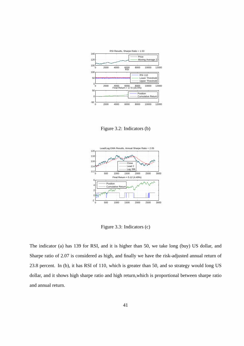
Figure 3.2: Indicators (b)
0 500 1000 1500 2000 2500 3000112
114
116
118
120Lead/Lag EMA Results, Annual Sharpe Ratio = 2.05
CloseLead 2Lag 396
0 500 1000 1500 2000 2500 3000-2
0
2
4
6Final Return = 5.12 (4.49%)
PositionCumulative Return
Figure 3.3: Indicators (c)
The indicator (a) has 139 for RSI, and it is higher than 50, we take long (buy) US dollar, and
Sharpe ratio of 2.07 is considered as high, and finally we have the risk-adjusted annual return of
23.8 percent. In (b), it has RSI of 110, which is greater than 50, and so strategy would long US
dollar, and it shows high sharpe ratio and high return,which is proportional between sharpe ratio
and annual return.
41

0 500 1000 1500 2000 2500 3000110
115
120RSI Results, Sharpe Ratio = -0.891
PriceMoving Average 2
0 500 1000 1500 2000 2500 30000
50
100RSI
RSI 110Lower ThresholdUpper Threshold
0 500 1000 1500 2000 2500 3000-5
0
5Final Return = -2.23 (-1.95%)
PositionCumulative Return
Figure 3.4: Indicators (d)
0 500 1000 1500 2000 2500 3000110
115
120MA+RSI Results, Sharpe Ratio = 0.204
PriceLead 2Lag 396Mov. Avg.2
0 500 1000 1500 2000 2500 30000
50
100RSI
RSI 110Lower ThresholdUpper Threshold
0 500 1000 1500 2000 2500 3000-5
0
5Final Return = 0.51 (0.447%)
PositionCumulative Return
Figure 3.5: Indicators (e)
The indicator (d) shows negative sharpe ratio and negative return, and in figure 11, we have lower
sharpe ratio and lower return than ones of figure 1 through (e). It demonstrate that the higher
sharpe ratio is equivalent to higher annual return, which is corresponding.
In (c), we have annual sharpe ratio of 2.05 but final return of 5.12 percent, which is lower than
42

the others with sharpe ratio close to 2.05. It means that even though we have good sharpe ratio,
we can have lower profits, and it means that one indicator cannot be perfect to anticipate optimal
investment strategy. So we collect and analyze the pros and cons of all indicators, we have to apply
the best investment strategy. The results is Table 4.1.
43

CHAPTER 4: CONCLUSION
In optimal control and HJB equation section, we found Lemma (Obstacle) on page 27, and it shows
that in mathematically how market making should work to attain optimal strategy.
In statistical arbitrage section, we found the strategy of Table 4.1.
Table 4.1: investment strategy
Indicators MV EMA RSI Sharperesponse to price fluctuation slow quick middle middle
suitable investment time long short short middleerror middle high middle middle
past data connection middle strong middle middlecalculation middle middle middle easy
trending market needed middle middle weakly trending strongly trending
The indicator (c) has its investment time interval of 3000 minutes, but the other figures have invest-
ment time of 12,000 minutes. Table 4.1 shows that EMA and RSI are suitable for short investment
time and MV is ideal indicator for long investment time. Thus, for 3000 minutes it is better to use
EMA or RSI to find more exact analysis.
44

APPENDIX : CODE FOR FIGURES OF CHAPTER 3
45

load bund1min testPts = floor(0.8*length(data(:,4))); step = 30; BundClose = data(1:step:testPts,4);
BundCloseV = data(testPts+1:step:end,4); annualScaling = sqrt(250*60*11/step); cost = 0.01;
rs = rsindex(BundClose,14); plot(rs), title(’RSI’)
rs2 = rsindex(BundClose-movavg(BundClose,30,30),14); hold on plot(rs2,’g’) legend(’RSI on raw
data’,’RSI on detrended data’) hold off
rsi(BundClose,[15*20,20],65,annualScaling,cost)
range = 1:300,1:300,55; rsfun = @(x) rsiFun(x,BundClose,annualScaling,cost); tic [ ,param] =
parameterSweep(rsfun,range); toc rsi(BundClose,param(1:2),param(3),annualScaling,cost)
rsi(BundCloseV,param(1:2),param(3),annualScaling,cost)
N = 10; M = 394; [sr,rr,shr] = rsi(BundClose,param(1:2),param(3),annualScaling,cost)
; [sl,rl,shl,lead,lag] = leadlag(BundClose,N,M,annualScaling,cost);
s = (sr+sl)/2; r = [0; s(1:end-1).*diff(BundClose)-abs(diff(s))*cost/2]; sh = annualScaling*sharpe(r,0);
figure ax(1) = subplot(2,1,1); plot([BundClose,lead,lag]); grid on legend(’Close’,[’Lead ’,num2str(N)]
, [’Lag’,num2str(M)],’Location’,’Best’)
title([’MA+RSI Results, Annual Sharpe Ratio = ’,num2str(sh,3)]) ax(2) = subplot(2,1,2)
; plot([s,cumsum(r)]); grid on legend(’Position’,’Cumulative Return’,’Location’,’Best’)
title([’Final Return = ’,num2str(sum(r),3),’ (’,num2str(sum(r)/BundClose(1)*100,3),’linkaxes(ax,’x’)
marsi(BundClose,N,M,param(1:2),param(3),annualScaling,cost)
range = 1:10, 350:400, 2:10, 100:10:140, 55; fun = @(x) marsiFun(x,BundClose,annualScaling,cost);
tic [maxSharpe,param,sh] = parameterSweep(fun,range); toc
46

param
marsi(BundClose,param(1),param(2),param(3:4),param(5),annualScaling,cost)
marsi(BundCloseV,param(1),param(2),param(3:4),param(5),annualScaling,cost)
47

LIST OF REFERENCES
[1] Almgren and Chriss, (2000): Optimal execution of portfolio transactions. J. Risk, 3(2):5-39
[2] AFM, 2010, High frequency trading: The application of advanced trading technology in the
European marketplace
[3] The Real Story of Trading Software Espionage (07.10.2009), Advanced Trading
[4] Avellaneda M. and S. Stoikov (2008): High frequency trading in a limit order book”, Quanti-
tative Finance, 8(3), 217-224.
[5] Basak and G. Chabakauri (2010): Dynamic mean-variance asset allocation. Rev. Financial
Studies, 23(8):2970-3016
[6] Bayraktar E. and M. Ludkovski (2011): ”Liquidation in limit order books with controlled
intensity”, available at: arXiv:1105.0247
[7] http://www.businessinsider.com/3-advantages-of-high-frequency-trading-2012-9
[8] R.Bielecki, H. Jin, S. R. Pliska, and Z. Y. Zhou (2005): Continuous-time mean variance
portfolio selection with bankruptcy prohibition. Math Finance, 15(2):213-244
[9] DeBondt, W., Thaler, R. (1985). Does the Stock Market Overreact? Journal of Finance, 40,
793-808.
[10] Cartea A. and S. Jaimungal (2011): ”Modeling Asset Prices for Algorithmic and High Fre-
quency Trading”, preprint University of Toronto.
[11] ”Advances in High Frequency Strategies”, Complutense University Doctoral Thesis (pub-
lished), December 2011, retrieved 2012-01-08
48

[12] Cont R., Stoikov S. and R. Talreja (2010): ”A stochastic model for order book dynamics”,
Operations research, 58, 549-563.
[13] Engelberg, J, Gao, P and R. Jaggannathan (2009): An anatomy of Pairs trading: the role of
idiosyncratic news, common information and liquidity; unpublished.
[14] A. Forsyth (2011): A Hamilton-Jacobi-Bellman approach to optimal trade execution. Appl.
Numer. Math., 61(2):241-265
[15] Gatev, Evan, William N.Goetzmann and K. Geert Rouwenhorst (2006): Pairs Trading: Per-
formance of a Relative-Value Arbitrage, Review of Financial Studies 19, 797-827
[16] Gervais, Simon. Ron Kaniel, and Dan H. Mingelgrin, (2001): The High-Volume Return Pre-
mium, The Journal of Finance 56, 877-919.
[17] Gatev, Evan, William N. Goetzmann, and K. Geert Rouwenhorst, 2006, Pairs Trading: Per-
formance of a Relative-Value Arbitrage, Review of Financial Studies 19, 797 - 827.
[18] Geoffrey Rogow,Eric Ross Rise of the (Market) Machines, The Wall Street Journal, June 19,
2009
[19] Gueant O., Fernandez Tapia J.and C.-A. Lehalle (2011): ”Dealing with inventory risk”,
preprint.
[20] Guilbaud, Fabien and Pham, Huyen: ”Optimal High Frequency Trading with Limit and Mar-
ket Orders” (2011). Available at SSRN: http://ssrn.com/abstract=1871969
[21] H. He and H. Mamaysky. Dynamic trading policies with price impact. J. Econom. Dynam.
Control, 29(5):891-930, 2005
[22] T. Ho and H. Stoll, Optimal Dealer Pricing under Transactions and Return Uncertainty, Jour-
nal of Financial Economics, 9 (1981) 47-73.
49
[23] Hong, Harrison, and Jeremy C. Stein, 1999, A uni.ed theory of underreaction, momentum
trading, and overreaction in asset markets, Journal of Finance, Vol 54, 2143-2184.
[24] Irene Aldridge (July 8, 2010). ”What is High Frequency Trading, After All?”. Huffington
Post. Retrieved August 15, 2010.
[25] Aldridge, Irene (2009), High-Frequency Trading: A Practical Guide to Algorithmic Strate-
gies and Trading Systems (Wiley), ISBN 978-0-470-56376-2
[26] ”Regulatory Issues Raised by the Impact of Technological Changes on Market Integrity and
Efficiency”, IOSCO Technical Committee, July 2011, retrieved 2011-07-12
[27] Jegadeesh, N., Titman, S. (1993). Returns to Buying Winners and Selling Losers: Implica-
tions for Stock Market Efficiency. Journal of Finance, 48(1), 65-91.
[28] Jiongmin Yong, Xun Yu Zhou, ”Stochastic Controls: Hamiltonian Systems and HJB Equa-
tions” Springer — 1999 — ISBN: 0387987231
[29] ”The Microstructure of the Flash Crash: Flow Toxicity, Liquidity Crashes and the Probability
of Informed Trading”, Journal of Portfolio Management, October 2010, retrieved 2012-01-08
[30] Julian Lorenz and RA, ”Mean-variance optimal adaptive execution”, Applied Mathematical
Finance 18 (2011) 395-422.
[31] David Kane, Andrew Liu and Khanh Nguyen,2011, Analyzing an Electronic Limit Order
Book
[32] Kuhn C. and M. Stroh (2010): ”Optimal portfolios of a small investor in a limit order market:
a shadow price approach”, Mathematics and Financial Economics, 3(2), 45-72.
[33] Lehmann, Bruce, 1990, Fads, Martingales and Market Efficiency, Quarterly Journal of Eco-
nomics 105, 1.28.
50

[34] Li and W. L. Ng (2000): Optimal dynamic portfolio selection: Multiperiod mean variance
formulation. Math. Finance, 10(3):387-406
[35] http://blog.naver.com/mhbae200?Redirect=Log
[36] http://www.quantshare.com/sa-90-sharpe-ratio-part-2 ixzz2HGoOeq00
[37] R.Richardson (1989): A minimum variance result in continuous trading portfolio optimiza-
tion. Management Science, 35(9): 1045-1055
[38] Sal L. Arnuk and Joseph Saluzzi (2008) : Toxic Equity Trading Order Flow on Wall Street A
Themis Trading LLC White Paper
[39] Schied and T. Schoneborn (2009): Risk aversion and the dynamics of optimal liquidation
strategies in illiquid markets. Finance Stochast., 13(2):181-204
[40] ”Trade Worx / SEC letters”. April 21, 2010. Retrieved September 10, 2010.
[41] Stuart Kozola(2010), Algorithmic Trading with MATLAB(R)2010: Moving Average and
RSI.
[42] Thomas C Shik and Terence Tai-Leung Chong (2007) A Comparison of MA and RSI returns
with exchange rate intervention, Applied Economics Letters, 2007, 14, 371 - 383.
[43] Veraart L.A.M. (2011): ”Option market making under inventory risk”, Review of Derivatives
Research, 12(1), 55-79
[44] Veraart L.A.M. (2011): ”Optimal Investment in the Foreign Exchange Market with Propor-
tional Transaction Costs”, Quantitative Finance, 11(4): 631-640. 2011.
[45] http://www.youtube.com/watch?v=FGHbddeUBuQ What is High Frequency Trading (video)
51

[46] Y. Zhou and D. Li (2000): ”Continuous-time mean-variance portfolio selection: A stochastic
LQ framework”. Appl. Math. Optim., 42:19-33
52