hiwire progress report chania, may 2007 presenter: prof. alex potamianos technical university of...
Post on 20-Dec-2015
231 views
TRANSCRIPT
HIWIRE Progress ReportChania, May 2007
Presenter: Prof. Alex PotamianosTechnical University of Crete
Presenter: Prof. Alex PotamianosTechnical University of Crete

Audio-Visual Processing (WP1) VTLN (WP2)
Segment Models (WP1) Recognition on BSS (WP1) Bayes’ Optimal Adaptation (WP2)
Outline
Audio-Visual Processing (WP1) VTLN (WP2)
Segment Models (WP1) Recognition on BSS (WP1) Bayes’ Optimal Adaptation (WP2)
Outline
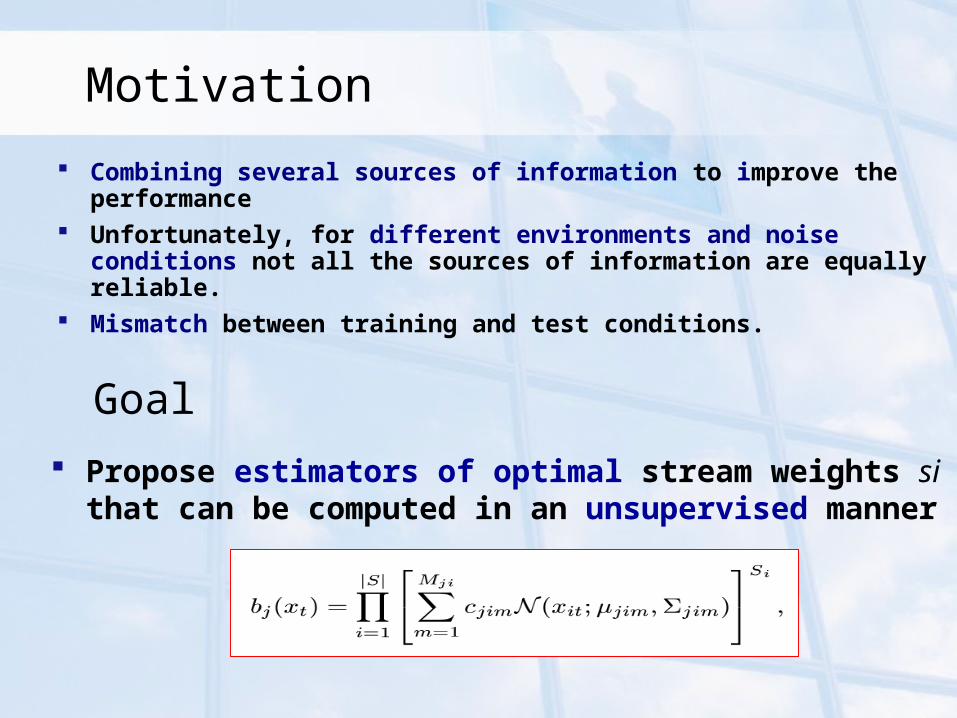
Combining several sources of information to improve the performance
Unfortunately, for different environments and noise conditions not all the sources of information are equally reliable.
Mismatch between training and test conditions.
Goal
Propose estimators of optimal stream weights si that can be computed in an unsupervised manner
Motivation

Equal error rate in single-stream classifiers
Equal estimation error variance in each stream
Optimal Stream Weights
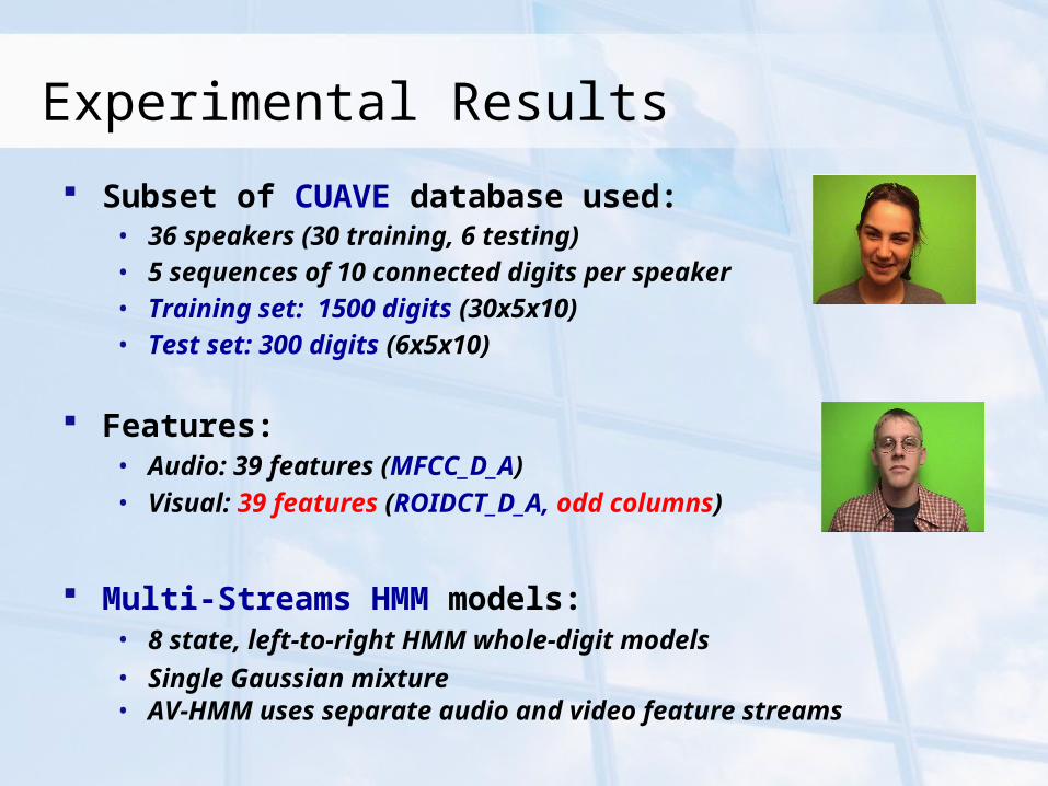
Subset of CUAVE database used:• 36 speakers (30 training, 6 testing)• 5 sequences of 10 connected digits per speaker • Training set: 1500 digits (30x5x10)• Test set: 300 digits (6x5x10)
Features: • Audio: 39 features (MFCC_D_A)• Visual: 39 features (ROIDCT_D_A, odd columns)
Multi-Streams HMM models:• 8 state, left-to-right HMM whole-digit models
• Single Gaussian mixture• AV-HMM uses separate audio and video feature streams
Experimental Results

,);(/);2,1(
);(/);2,1(
1intrainter
2intrainter
2
1
ij
ij
jidjd
jidjdfc
s
s
Two classes →
anti models Class membership →
inter and intra classes distance
Results (classification)

Generalization of the inter- and intra-distances measure → inter distance among all the classes.
int int1 1
( ) ( , ; )K K
k l k
d j d k l j
Results (recognition)

Stream weight computation for • multi class classification task • based on theoretical results for a two classes classification• use of an anti-model technique
We use only the test utterance and the information contained in the trained models.
Generalization towards unsupervised estimation of stream weights for multi-streams classification and recognition problems.
Conclusions
Audio-Visual Processing (WP1) VTLN (WP2)
Segment Models (WP1) Recognition on BSS (WP1) Bayes’ Optimal Adaptation (WP2)
Outline
Vocal Tract Length Normalization.
Dependence between warping and phonemes. Frame Segmentation into Regions. Warping Factor and Function Estimation. VTLN in Recognition. Evaluation.
Dependence between warping and phonemes[1].
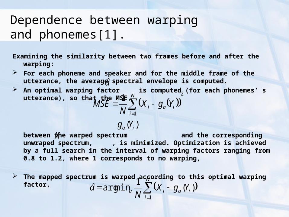
Examining the similarity between two frames before and after the warping: For each phoneme and speaker and for the middle frame of the utterance, the
average spectral envelope is computed. An optimal warping factor is computed (for each phonemes’ s utterance), so
that the MSE,
between the warped spectrum and the corresponding unwraped spectrum, , is minimized. Optimization is achieved by a full search in the interval of warping factors ranging from 0.8 to 1.2, where 1 corresponds to no warping,
The mapped spectrum is warped according to this optimal warping factor.
a
2
1
1
N
iiai YgX
NMSE
)( ia YgX
2
1
)(1
minargˆ
N
iiaia YgX
Na
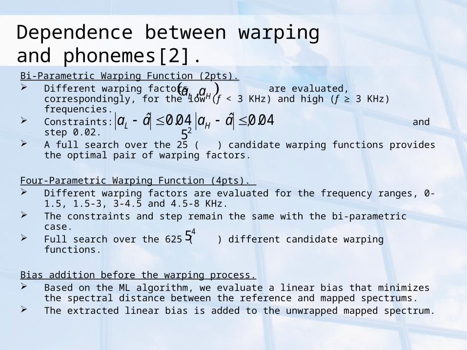
Dependence between warping and phonemes[2].Bi-Parametric Warping Function (2pts). Different warping factors are evaluated, correspondingly, for the
low (f < 3 KHz) and high (f ≥ 3 KHz) frequencies. Constraints: , and step 0.02. A full search over the 25 ( ) candidate warping functions provides the
optimal pair of warping factors.
Four-Parametric Warping Function (4pts). Different warping factors are evaluated for the frequency ranges, 0-1.5, 1.5-
3, 3-4.5 and 4.5-8 KHz. The constraints and step remain the same with the bi-parametric case. Full search over the 625 ( ) different candidate warping functions.
Bias addition before the warping process. Based on the ML algorithm, we evaluate a linear bias that minimizes the
spectral distance between the reference and mapped spectrums. The extracted linear bias is added to the unwrapped mapped spectrum.
04.0ˆ aaL25
45
04.0ˆ aaH
HL aa ,

Results (over all speakers) after bias addition.

Frame Segmentation into Regions.
Based on unsupervised K-Means algorithm, a sequence of testing utterance’s
frames, length M, is divided on, specific by us, population of regions.
The algorithm’s output is a function F between the frames m and the
corresponding region index c,
As an additional constraint, a media filtering is placed on the region index’s
sequence. This constraint has the effect of smoothing the sequence of indices so
as to reflect a more physiologically degree of region transition between
successive frames.
:F m c
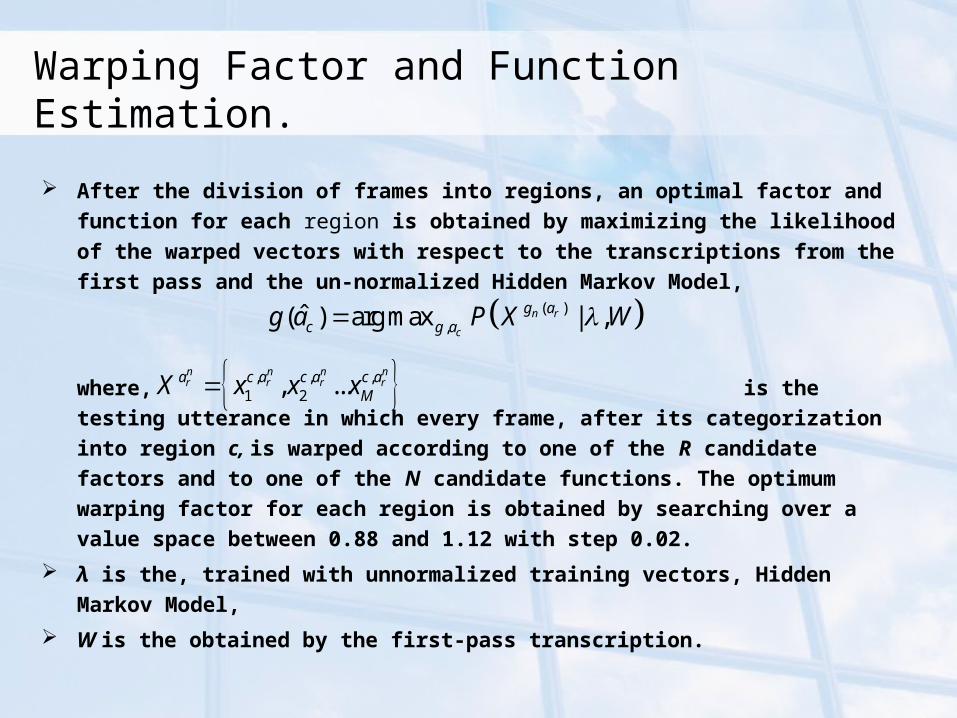
Warping Factor and Function Estimation.
After the division of frames into regions, an optimal factor and function for each
region is obtained by maximizing the likelihood of the warped vectors with
respect to the transcriptions from the first pass and the un-normalized Hidden
Markov Model,
where, is the testing utterance in which every frame,
after its categorization into region c, is warped according to one of the R
candidate factors and to one of the N candidate functions. The optimum warping
factor for each region is obtained by searching over a value space between 0.88
and 1.12 with step 0.02.
λ is the, trained with unnormalized training vectors, Hidden Markov Model,
W is the obtained by the first-pass transcription.
( ),ˆ( ) arg max | ,n r
c
g ac g ag a P X W
, , ,1 2, ...
n n n nr r r ra c a c a c a
MX x x x
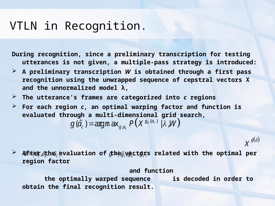
VTLN in Recognition.
During recognition, since a preliminary transcription for testing utterances is not given, a multiple-pass strategy is introduced:
A preliminary transcription W is obtained through a first pass recognition using the unwrapped sequence of cepstral vectors X and the unnormalized model λ,
The utterance's frames are categorized into c regions
For each region c, an optimal warping factor and function is evaluated through a multi-dimensional grid search,
After the evaluation of the vectors related with the optimal per region factor
and function the optimally warped sequence is decoded in order to obtain the final recognition result.
( ),ˆ( ) arg max | ,n r
c
g ac g ag a P X W
1 2ˆ ˆ ˆ ˆ, Ca a a a
1 2ˆ ˆ ˆ ˆ, Cg g g g
ˆ ˆg aX

Results
WER(%)
# of Utters 1 5
Baseline 50.83
Li & Rose (2 pass)
43.79 43.48
2 regions 41.73 (+4.7%) 42.79 (+1.60)
3 regions 43.11 (+1.56) 43.66 (-0.46)
Audio-Visual Processing (WP1) VTLN (WP2)
Segment Models (WP1) Recognition on BSS (WP1) Bayes’ Optimal Adaptation (WP2)
Outline

The Linear Dynamic Model (LDM)
Discrete-time Linear Dynamical Systems:
Efficient model the evolution of spectral dynamics An observation yk is produced in each time step The state process is first-order Markov
• Initial state is Gaussian The state and observation noises wk , vk are:
• Uncorrelated• Temporally white• Zero-mean Gaussian distributed
1 ~ (0, )
~ (0, )k k k k
k k k k
x Fx w w N Q
y Hx v v N R

Noise covariances are not constrained Matrices F,H have canonical forms
Canonical form is identifiable if it is also controllable (Ljung)
Generalized canonical form of LDM
0 1 0 0 0
1 0 0 0 0
0 0 1 0 0
0 0 0 1 00 0 0 0 1
F H

Experimental Setup
Training Set• Aurora 2 Clean Database• 3800 training sentences
Test set:• Aurora 2, test A, subway sentences • 1000 test sentences• Different levels of noise (Clean, SNR: 20, 15, 10, 5 dB)
Front-End extracts 14-dimensional features (static features):• HTK standard front-end• 2 feature configurations
– 12 Cepstral Coefficients + C0 + Energy– + first and second order derivatives (δ, δδ)

Model Training on Speech Data Word models with different number of segments based on
the phonetic transcription
Segment alignments produced using HTK
Segments Models
2 oh
4 two, eight
6 one, three, four, five, six, nine, zero
8 seven

Classification process
Keep true word-boundaries fixed • Digit-level alignments produced by an HMM
Apply suboptimum search and pruning algorithm• Keep the 11 most probable word-histories for each
word in the sentence
Classification is based on maximizing the likelihood
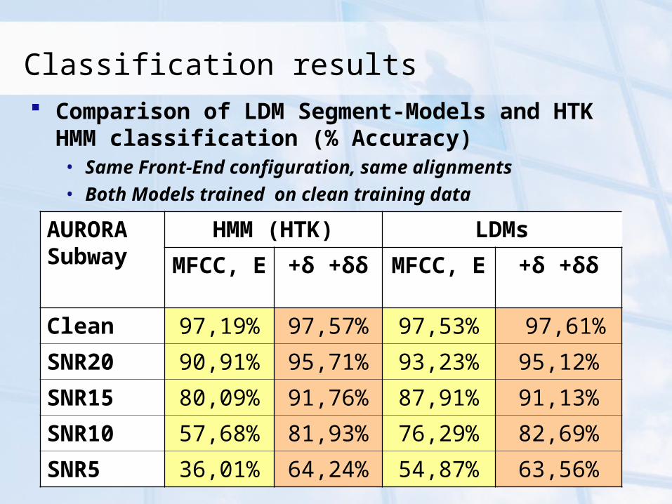
Classification results Comparison of LDM Segment-Models and HTK
HMM classification (% Accuracy)• Same Front-End configuration, same alignments• Both Models trained on clean training data
AURORASubway
HMM (HTK) LDMs
MFCC, E +δ +δδ MFCC, E +δ +δδ
Clean 97,19% 97,57% 97,53% 97,61%
SNR20 90,91% 95,71% 93,23% 95,12%
SNR15 80,09% 91,76% 87,91% 91,13%
SNR10 57,68% 81,93% 76,29% 82,69%
SNR5 36,01% 64,24% 54,87% 63,56%

Classification results
Performance Comparison (MFCCs)
Observation: 14 MFCCs
0
20
40
60
80
100
120
clean 20 15 10 5
SNR
Acc
ura
cy %
HMM
LDM
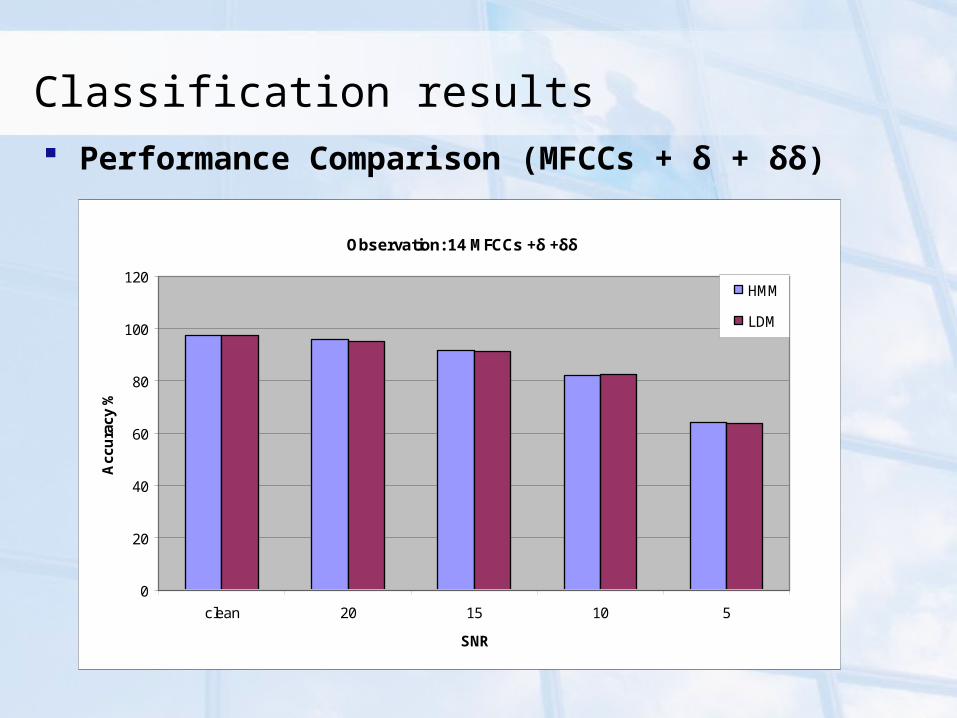
Classification results Performance Comparison (MFCCs + δ + δδ)
Observation: 14 MFCCs +δ +δδ
0
20
40
60
80
100
120
clean 20 15 10 5
SNR
Acc
ura
cy %
HMM
LDM

Sub-optimal Viterbi decoding (SOVD)
We use a Viterbi-like decoding algorithm for speech classification HMM state equivalent in LDMs is : [xk,si]
It is applied among the segments of each word-model• Provides segment alignments based on the likelihood of the LDM• Estimated with a Kalman filter
• Allows decoding at each time k using possible histories leading to a different [xk,si] combination at several depth levels
1( , ) log | ( ) | ( ) ( )k k
Tk e k e kL y e e C

SOVD Steps
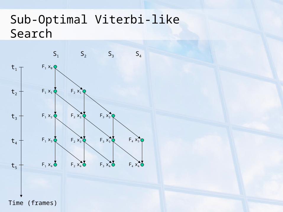
Sub-Optimal Viterbi-like Search
S2S1 S3 S4
F1 x0
F1 x1
F1 x2
F1 x3
F1 x4
F2 x1
F2 x2
F2 x3
F2 x4
F3 x2
F3 x3
F3 x4
F4 x3
F4 x4
t1
t2
t4
t5
t3
Time (frames)
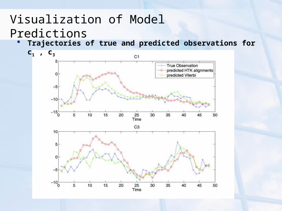
Visualization of Model Predictions Trajectories of true and predicted observations for c1 , c3

Classification results
Comparison of Segment-Models and HTK HMM classification (% Accuracy)• Same fixed Word-boundaries based on the HMM alignments
• Same Front-End configuration
• Both Models trained on clean training data
AURORASubway
HMM-alignments Segment Models
HMM LDM d=1 d=2
Clean 97,19% 97,85% 97,73% 97,76%
SNR20 90,91% 92,53% 93,52% 93,52%
SNR15 80,09% 85,93% 89,68% 89,77%
SNR10 57,68% 71,30% 77,21% 77,33%
SNR5 36,01% 46,72% 53,66% 53,98%
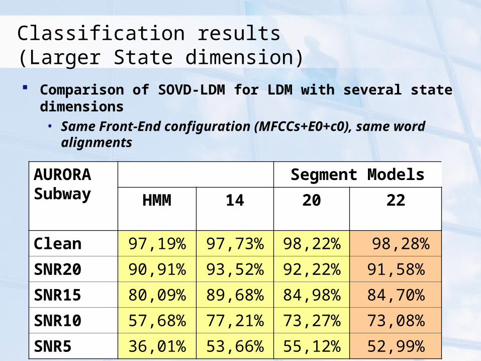
Classification results (Larger State dimension) Comparison of SOVD-LDM for LDM with several state
dimensions• Same Front-End configuration (MFCCs+E0+c0), same word
alignments
AURORASubway
Segment Models
HMM 14 20 22
Clean 97,19% 97,73% 98,22% 98,28%
SNR20 90,91% 93,52% 92,22% 91,58%
SNR15 80,09% 89,68% 84,98% 84,70%
SNR10 57,68% 77,21% 73,27% 73,08%
SNR5 36,01% 53,66% 55,12% 52,99%

Conclusions
We investigated generalized canonical forms for LDM
We proposed an element-wise ML estimation process
When alignments from an equivalent HMM• Without derivatives LDMs significantly outperform
HMMs particularly under highly noisy conditions
• When derivatives are used for both models their performance is similar

Conclusions
With segment alignments based on LDM• HMM alignments hurt recognition performance• Viterbi-like search for LDM
Larger-dimension• Beneficial on clean data• Performance degrades on noisy data
Future• Lower-dimension, articulatory-based features• Non-linear state-to-observation mappings

Audio-Visual Processing (WP1) VTLN (WP2)
Segment Models (WP1) Recognition on BSS (WP1) Bayes’ Optimal Adaptation (WP2)
Outline
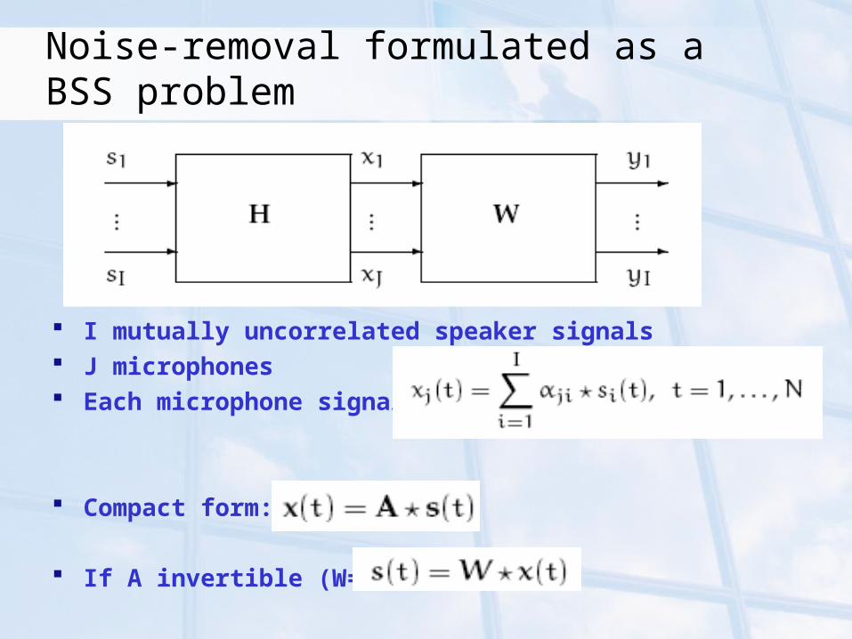
Noise-removal formulated as a BSS problem
I mutually uncorrelated speaker signals J microphones Each microphone signal :
Compact form:
If A invertible (W=A-1):

The simulated room
Used Douglas Cambell’s “Roomsim” Depicts the positions of the speakers and mics
Mixed file was the one received by the first mic (top left)

Database
We considered Aurora 4 and TIMIT BSS shows better separability fo speech
signals >30s• Aurora 4 average utterance length ~7sec• TIMIT average utterance length ~3sec• Concatenated sentences of the same speakers
When there was no overlapping during the whole time• We replicated the smaller sentence with samples
from the beginning We normalized the sources to ensure same
energy
Experimental Setup
Test Set: • 330 Utterances (AURORA4)• 16KHz – 16bits
Performance of the clean test-set: 11.13%
Results

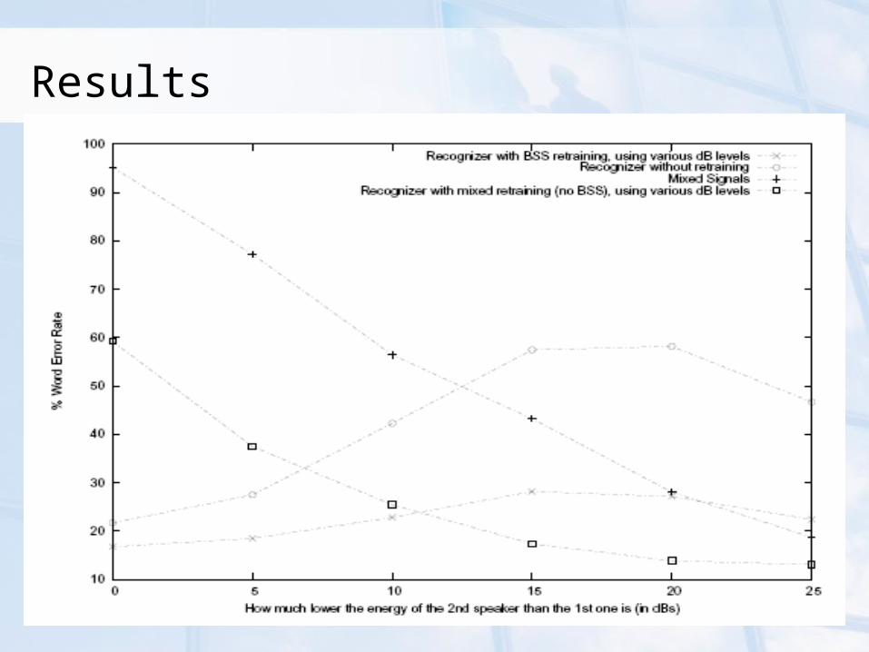
Conclusions Baseline model (with Spectral Subtraction) fails to
separate the signals Retraining the recognizer with mixed signals can
significantly improve performance for small noise levels
BSS test data and Baseline model• Significantly reduces WER when the speaker’s signal is at
the same level• Performance highly degrades as the energy of the second
speaker decreases. BSS test data + Retrained models with BSS data
• Best performance for noise levels 10dB or lower For smaller noise levels (>10dB) use the recognizer
retrained on mixed signals rather than BSS
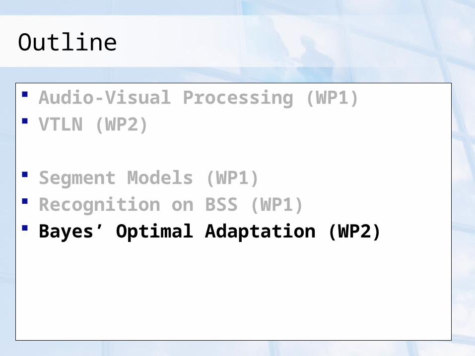
Audio-Visual Processing (WP1) VTLN (WP2)
Segment Models (WP1) Recognition on BSS (WP1) Bayes’ Optimal Adaptation (WP2)
Outline

We want to determine
Weighted average of many estimators
In our approach θ denotes a Gaussian component
• Θ is a subset of Gaussians
Optimal Bayes Adaptation
1 1
| , , | , | , | ,N N
t t A t A t t A t A t
R R
p x s X p x X s d p x X s p X s d
1
( | , ) ( ) ( ; , ) ( | , )M
t t a i t t i i a ti
p x s X c s N x m S p X s
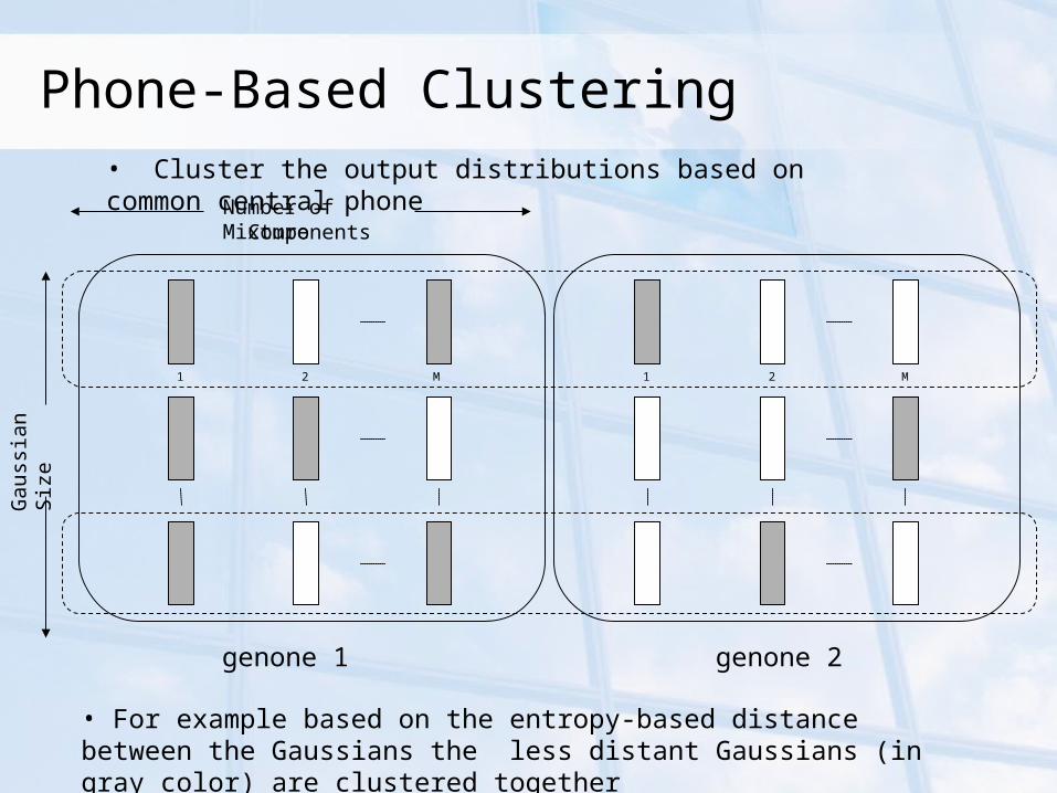
1 2 M 1 2 M
genone 1 genone 2
Phone-Based Clustering
• Cluster the output distributions based on common central phone
• For example based on the entropy-based distance between the Gaussians the less distant Gaussians (in gray color) are clustered together
Gau
ssia
n S
ize
Number of MixtureComponents

Likelihoods Collection
We compute the likelihoods by using
For each voice frame we track which triphones are used and calculate the probability for each θ.
We use delta smoothing to the distributions of θ according to
1 1
| , ( ) | , ( )T T
A t A t At t
p X s p x t s b x t
_
Np k
N total symbols

Baseline trained on the WSJ database
Adaptation data: • spoke3 WSJ task• non-native speakers• 5 male and 5 female• 40 adaptation sentences per speaker• 40 test sentences per speaker
Adaptation Configuration

Results
Comparison of 6-Associations and Baseline
39.00%
40.00%
41.00%
42.00%
43.00%
44.00%
45.00%
46.00%
47.00%
Baseline 6-Associations
WE
R%
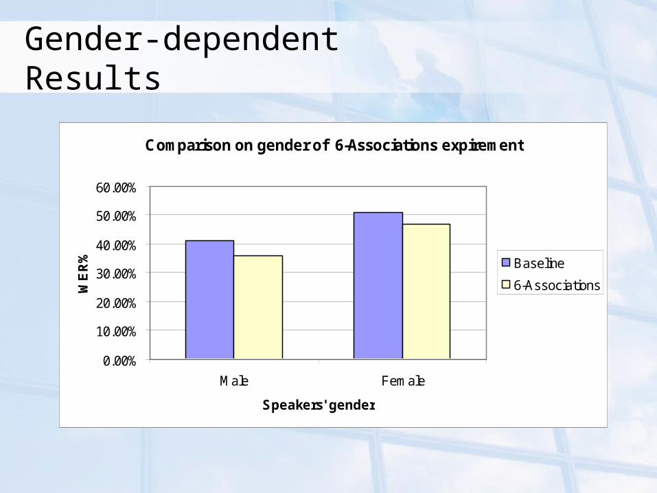
Gender-dependent Results
Comparison on gender of 6-Associations expirement
0.00%
10.00%
20.00%
30.00%
40.00%
50.00%
60.00%
Male Female
Speakers' gender
WE
R% Baseline
6-Associations

Conclusions
A small improvement compared to the baseline case
Recent experiments have shown that dynamic associations of distributions have better results
Increasing the number of adaptation data improves the recognition results as recent experiments have shown.