History Matching of Petroleum Reservoirs Using a

Level Set Technique

Oliver Dorn and Rossmary Villegas

Modelling and Numerical Simulation Group, Universidad Carlos III de Madrid,Avenida de la Universidad 30, Leganes 28911, Spain

Abstract.We describe a novel technique for the characterization of structured reservoirs from

production data. A level set technique is used in order to be able to incorporateinterfaces between different lithofacies in the reservoir. The new algorithm is ableto reconstruct, in addition to the shapes and topologies of the individual lithofacies,also their internal permeability profiles simultaneously from the given production data.Here either a pixel-by-pixel or a parameterized model can be used for describing each ofthe internal profiles, and any hybrid combination of them. If n lithofacies are presentin the reservoir, n − 1 level set functions are employed during the characterization.Overlapping regions of these n − 1 level set functions are treated by a specialtechnique tailored to the reservoir characterization application. Here our approachdiffers significantly from standard techniques for describing more than two values bya level set representation. We also describe techniques for testing the existence andcharacteristic features of certain geometrical structures (such as channels or barriers)inside the reservoir by suitable topological perturbations of the describing level setfunction. Numerical results in 2D are presented which demonstrate the performanceof our novel scheme for a variety of simulated but realistic situations which are ofimportance in reservoir engineering applications.

Submitted to: Inverse Problems

2

1. Introduction

Reservoir characterization by history matching of production data has a long history,

see for example the contributions [1, 3, 5, 10, 11, 13, 14, 27, 30] and the many references

given there. The reservoir engineer needs to understand the geological properties inside

the Earth in order to optimize the production process of active oil fields. Certainly, the

Earth has a very complex structure and it is impossible to determine from few production

data all the details of the reservoir. On the other hand, it would be desirable to be

able to identify at least some important large-scale structural features of the reservoir.

For example, many reservoirs are composed of different geological regions (lithofacies)

which are separated by clearly defined interfaces or contain certain channel or barrier

structures. Some of these interfaces can be determined by analysis of seismic data, but

not all of them. Traditional history matching techniques are not able to resolve these

interfaces due to the way these tools are constructed. Typically an inverse problem is

solved for determining pixel-values (voxel-values in 3D applications) of petrophysical

parameters (e.g. porosity and permeability) inside the reservoir which minimize,

when plugged into a reservoir simulator, the mismatch between simulated and actual

production data in some sense. Due to the need of very strong regularization (caused by

the ill-posedness of the inverse problem and the sparsity of available production data)

in most cases an oversmoothed reconstruction is delivered from which it is impossible

to detect any clearly defined region boundaries without additional image segmentation

tools. Image segmentation techniques, on the other hand, typically change these profiles

without taking into account production data, such that the segmented images do not

honor anymore production data and are therefore -to the least- suboptimal.

In this work we present a novel reservoir characterization technique which aims at

directly providing structured profiles of physical parameters (here permeability) from

production data without the need of any segmentation postprocessing techniques. In

addition, our technique is able to incorporate smoothly varying region-internal profiles

in each area of the reservoir.

Another important aspect of reservoir characterization is that the history matching

problem typically is vastly underdetermined and that a unique solution does not exist.

Therefore, in order to plan future oil production, it is often desirable to have not just

one reconstruction available (given for example by a classical Tikhonov-Philips scheme)

which honors the available information, but a broad variety of possible reconstructions.

Traditional reservoir characterization techniques yield typically those reconstructions

which do not incorporate any interfaces. In this sense, our technique is intended to be

a generalization of classical history matching techniques which adds the flexibility of

incorporating certain interfaces and therefore certain types of structural features into

the inversion which honor production data. The classical pixel-/voxel-based schemes

can then be considered as a special case of our new scheme where only one ’lithofacie’

(i.e. one region) is present in the reservoir.

For describing the fluid flow in the reservoir, we use a simplified two phase

3

incompressible flow model of oil and water [29]. We mention that the inversion algorithm

developed here can without problems be applied to more complex (e.g. three-phase flow)

models, as long as suitable forward and adjoint simulators are available for those models.

In order to avoid the so-called inverse crime, the data is generated with a streamline

method, while during the reconstruction process an independent IMPES method is used

to solve the forward problem. This guarantees that the ’exact’ solution, plugged into the

reservoir simulator, still produces simulated data which are sufficiently different from the

reference data which are used as input for the inversion. This makes the inversion process

more realistic, since reservoir simulators typically are not able to ’exactly’ reproduce real

data due to the various types of model and measurement noise included in real data.

We use a level set technique [2, 4, 9, 18, 19, 21, 22, 25, 26] for modeling interfaces of

regions with different geophysical properties in the Earth. The topology of the regions

separated by these interfaces is a-priori unknown. Using the available production data,

and some prior information from well-logs affecting physical parameters close to the well

locations, we try to recover a binary (or, in our generalized approach, multi-valued) map

of permeability values in the reservoir.

In the literature there exist several approaches focusing on alternative automatic

history matching techniques based on geological shape definitions. One example is

the use of shape triangularization [23, 24] which, however, requires to have prior

information of the topology and approximate facies locations available. Other methods

use geostatistical approaches [12, 20], which generally work well but are computationally

very expensive. Alternative level set based approaches have been proposed very recently

in the literature as well [15, 16, 17, 18]. Our scheme, as presented here, differs in several

aspects from those approaches. We apply a so-called ’adjoint scheme’ for calculating the

sensitivities during the reconstruction, we initialize the reservoir model using stochastic

and deterministic initializations based on prior information (parameter values measured

at the well locations), we allow for quite arbitrary internal permeability profiles during

the reconstruction task, we consider reservoirs with an arbitrary (but typically small)

number of different lithofacies, and we incorporate the possibility of testing the existence

and properties of certain geometrical objects in the reservoir. Moreover, as regularization

tool we use an adapted filtering operator to be applied in each step of the inversion

problem.

The paper is organized as follows. Following this section 1 where we have given a

short introduction into the history matching problem associated with geological shape

reconstruction in reservoir characterization, we present in section 2 the reservoir models,

specifically a mathematical description of the forward model and the adjoint model

which we use during the inversion process. Section 3 introduces into our inverse problem

and gives a theoretical derivation of the basic algorithms which we use for the inversion

of the geological shapes and internal profiles. As part of this section, subsection 3.1

presents the theoretical derivation of the basic algorithm for the automatic identification

of geological regions and, in addition, smoothly varying permeability distributions inside

these regions. The subsection 3.2 explains the regularization scheme which we apply in

4

our work for the reconstruction of the level set functions which describe the interfaces

between lithofacies. This regularization scheme basically assures that highly oscillating

parts of the final interfaces are avoided. In subsection 3.3 we focus on parameterized

internal permeability profiles. As a special case of that, in subsection 3.4 constant and

linearly varying profiles are briefly addressed. In section 4 we present our technique for

treating situations with more than two lithofacies. Here we introduce a new technique

which uses n − 1 level set functions for describing n lithofacies. Section 5 discusses

possibilities for adding objects with certain geometrical shapes to the reconstruction at

a given step of the evolution. For adding such an object we apply a perturbation to

the level set function which creates such an object without destroying the smoothness

properties of the level set function. In section 6 we present then various numerical

experiments which demonstrate the performance of the new techniques for simulated

but realistic situations, and in section 7 we give some conclusions.

2. The reservoir characterization problem

2.1. The reservoir model

Our simplified model for two-phase flow in porous media for reservoir engineering is

given as

φ∂Sw∂t

−∇ · [Tw(∇pw + ρwgk)] = Qw in Ω× [0, tf ] (1)

φ∂So∂t

−∇ · [To(∇po + ρogk)] = Qo in Ω× [0, tf ] . (2)

These two conservation laws for water (subscript w) and oil (subscript o), considered as

incompressible fluids in a porous medium, are typically augmented by the two additional

equations

Pcwo = po − pw, (3)

Sw + So = 1. (4)

This yields four equations (1)–(4) in the four unknowns pw, po, Sw and So. Hereafter,

the subindex ‘w’ stands for ’water’, and the subindex ‘o’ stands for ‘oil’. Equation (3)

links the water and oil pressures (pw and po, resp.) in the medium by the capillary

pressure Pcwo. Equation (4) links the saturations Sw of water and So of oil and indicates

that the porous medium is fully saturated. Gravity effects are taken into account by

the terms ρwgk and ρogk. These two terms, together with the capillary pressure Pcwo,

are incorporated in our forward modeling code, but are assumed to be small and will

be neglected when deriving the algorithm for solving the inverse problem. Ω ⊂ IRn

(n = 2, 3) is the modeling domain with boundary ∂Ω, and [0, tf ] is the time interval

for which production data is avalaible. We denote by φ(x) the porosity, and by To, Tw

5

and T the transmissibilities, which are known functions of the permeability K and the

water saturation Sw:

Tw = K(x)Krw(Sw)

µw; To = K(x)

Kro(Sw)

µo; T = Tw + To . (5)

Here, the relative permeabilities Krw(Sw) and Kro(Sw) are typically available as

tabulated functions, and µw and µo denote the viscosities of each phase. Qo, Qw and

Q = Qo + Qw define the oil flow, the water flow and the total flow, repectively, which

are measured at the well positions. Equations (1)-(4) are solved with appropriate initial

conditions, and a no-flux boundary condition on ∂Ω.

When neglecting the gravity terms ρwgk and ρogk, as well as capillary pressure

(such that pw = po = p), equations (1)–(4) simplify to the two equations

−∇ ·[T∇p

]= Q in Ω× [0, tf ] (6)

φ∂Sw∂t

−∇ · [Tw∇p] = Qw in Ω× [0, tf ] (7)

for the two unknowns p and Sw, where we add the following initial and boundary

conditions

Sw(x, 0) = S0w(x) in Ω , (8)

p(x, 0) = p0(x) in Ω , (9)

∇p · ν = 0 on ∂Ω . (10)

Here, ν is the outward unit normal to ∂Ω. The boundary condition (10) implies no flux

across the boundary. Equations (6)–(10) will be our basic model for deriving the shape

inversion algorithm. Q(x, t) and Qw(x, t) define the total flow and the water flow at the

wells, respectively. They are given by

Q = c T

Ni∑j=1

(p(i)wbj

− p)δ(x− x(i)j ) + c T

Np∑j=1

(p(p)wbj

− p)δ(x− x(p)j ) (11)

Qw = c T

Ni∑j=1

(p(i)wbj

− p)δ(x− x(i)j ) + c Tw

Np∑j=1

(p(p)wbj

− p)δ(x− x(p)j ) (12)

where x(i)j , j = 1, . . . , Ni, denote the locations of the Ni injector wells, x

(p)j , j = 1, . . . , Np,

denote the locations of the Np production wells, and p(i)wbj

, p(p)wbj

are the imposed well bore

pressures at the Ni injector wells and at the Np production wells, respectively. Here, c

is a constant that depends on the well model [6]. Since p(i)wbj

are larger than the reservoir

pressure at the injector wells, Q and Qw are positive at the injector wells. Similarly,

since p(p)wbj

are smaller than the reservoir pressure at the production wells, Q and Qw are

negative at the production wells.

In all the reservoir models discussed in this paper, there are two (incompressible)

fluids in the reservoir, water and oil. Certainly, all the techniques developed here can

6

easily be generalized to more complex reservoir models, which we intend to address in our

future research. We use tabulated values for the relative permeabilities Krw and Kro as

shown in [11], which correspond to a Corey function with coefficients nw = 3 and no = 2.

The viscosity values for oil and water are µo = 0.79× 10−3 Pa s and µw = 0.82× 10−3

Pa s, and the porosity is taken to be constant φ = 0.213 in the reservoir. The pressure

values in the reservoir are in the range between 2000 psi (imposed pressure at production

wells) and 3500 psi (imposed pressure at injection wells). The numerical physical time-

step (which is unrelated to the time-step of the artificial shape evolution) used in the

simulator is 0.1 days, and the reservoir is monitored over a period of 120 days. For more

details regarding our reservoir simulation tools, we refer again to [11].

2.2. The forward problem

We can now introduce the forward operator of our problem. We write equations (6)-(12)

in operator form as

Λ(K)u = q (13)

with u = (p, Sw) and where the right hand side q is defined by the right hand sides of

(6), (7), i.e., the expressions given in (11) and (12). Notice that the derivation of our

algorithm is not restricted to the assumption of wells modeled by point sources, and

that more complex descriptions of the wells (e.g., as interior boundary conditions) can

easily be incorporated in the algorithm. We can define the forward operator A mapping

the parameter K to the corresponding data g = Mu by

A(K) = M u(K) = M Λ(K)−1q (14)

where M is the measurement operator given by

Mu(K) = Q(p)w,j(K)j=1 ...,Np = Qw(K), (15)

being the water flow obtained at the production wells. Practically, calculating Λ(K)−1q

means to run our reservoir simulator on the applied input pressure data with the

permeability given as K. We will denote the physically measured ’true data’ by

g = Mu, (16)

where u denotes the (unknown) physical state given the correct parameter distribution

K. Finally, we introduce the ’residual operator’ R by defining

R(K) = A(K)− g = Qw(K)− Qw. (17)

2.3. The adjoint technique

The adjoint technique for reservoir characterization has been described in detail in

[5, 11, 14] (see also the many references given there) such that we recall here only the

main result as used in our implementations.

7

Let ρ ∈ D be an arbitrary function in the data space. Then R′(K)∗ρ is given by

R′(K)∗ρ =

∫ tf

0

(TwK∇p∇z − z

1

KQw

)dt (18)

where z is the solution of the adjoint problem

−φ∂z∂t

+∂Tw∂Sw

∇p∇z − (z −Np∑j=1

ρ δ(x− x(p)j ))

∂Qw

∂Sw= 0 in Ω (19)

z(x, tf ) = 0 in Ω, (20)

and Sw and p are the solutions of the forward problem (6)-(10), where both the forward

and the adjoint problem are solved with permeability distribution K.

Notice that Qw is nonzero only at the well locations. Therefore, when we assume

in the mathematical derivation of the theorem that the permeability is known directly

at the wells (these values are available from well-log data), the second term in (18)

disappears and we only have to evaluate the first term in order to calculate the update

in the rest of the domain Ω. This will be the approach we use in our numerical

reconstructions. For more details we refer to [11].

3. The shape reconstruction problem (two lithofacies)

3.1. General internal profiles

We start the description of our new technique by the simplest case where two lithofacies

are present in the reservoir. Classical history matching approaches typically formulate

a least squares cost functional of the type

J (K) =1

2‖R(K)‖2, (21)

possibly augmented by some additional regularization terms (e.g. of the Tikhonov-

Philips type) and try to find a (typically smoothly varying over the whole domain)

profile K(x) which minimizes this cost.

In the level set approach the two regions D and Ω\D are defined by a sufficiently

smooth level set function ψ in the following way [8]

K(x) =

Ki(x), if ψ(x) ≤ 0

Ke(x), if ψ(x) > 0 .(22)

Therefore, in our approach, we formulate a cost functional which does not, as in the

classical form, depend on a single (smoothly varying) function K but on three different

(e.g. smoothly varying) functions ψ, Ki and Ke

J(K) = J(K(ψ,Ki, Ke)) =1

2‖R(K(ψ,Ki, Ke))‖2. (23)

In our strategy, the level set function ψ will determine the interfaces between the two

regions present in the reservoir, whereas the functions Ki and Ke represent the internal

8

profiles in each of these regions. Notice that all three functions Ki, Ke and ψ are defined

on the entire reservoir, and that the function ψ determines at each location which of the

profiles Ki or Ke applies at this location. Therefore, in our extended inverse problem

there are three functions to be determined instead of one in the classical formulation.

Even though it seems a harder problem to find three functions now instead of just a

single profile in the classical approach, we will see that we gain much flexibility with this

extended approach. The increased dimensionality of the inverse problem can be dealt

with by applying suitable regularization tools when determining the three unknown

functions. We emphasize also that the classical case can be considered as a special

case of our model where the level set function is positive (or negative) over the entire

reservoir.

To solve the shape reconstruction problem, we will adopt a time evolution approach

[25]. As a consequence, ψ , Ke and Ki will be functions of an artificial evolution time t,

dψ

dt= f(x, t, ψ,R) (24)

dKi

dt= hi(x, t, ψ,R) ,

dKe

dt= he(x, t, ψ,R) . (25)

The goal is to determine the unknown terms f , hi and he such that the cost defined in

(23) decreases during the evolution. Using the one-dimensional Heaviside function, we

have

K = K(ψ,Ki, Ke) = KeH(ψ) + Ki(1−H(ψ)). (26)

Formal differentiation of the cost functional (23) with respect to the artificial time

variable t yields

dJdt

=dJdK

∂K

∂ψ

dψ

dt+dJdK

∂K

∂Ki

dKi

dt+dJdK

∂K

∂Ke

dKe

dt(27)

=

∫

Ω

R′(K)∗R(K)(∂K∂ψ

dψ

dt+∂K

∂Ki

dKi

dt+∂K

∂Ke

dKe

dt

)dx

by the chain rule. Here, the expression R′(K)∗R(K) is the adjoint of the linearized

residual operator (containing the sensitivities of the data with respect to the parameters)

applied to the most recent mismatch in the data. It can be calculated efficiently by using

the adjoint scheme outlined in section 2.3. The individual components of (27) can be

identified as ∂K∂ψ

= (Ke − Ki)δ(ψ), ∂K∂Ki

= 1 − H(ψ), and ∂K∂Ke

= H(ψ), where we have

used that the derivative of the one-dimensional Heaviside function H(ψ) is the one-

dimensional Dirac delta function δ(ψ). We can select descent directions for the cost

functional by defining

fSD = −C1χNB(ψ)(Ke −Ki)R′(K)∗R(K) (28)

hiSD = −C2(1−H(ψ))R′(K)∗R(K) (29)

heSD = −C3H(ψ)R′(K)∗R(K) . (30)

9

This can be verified by plugging these expressions into equation (27) for dJdt

. Here,

C1, C2, C3 are some small (possibly time-dependent) positive constants (which also

can be zero) modifying the evolution speed of these quantities individually. The

function χNB(ψ) has values 1 in a small neighborhood centered around the zero level

set (the so-called ’narrowband’) and zeros elsewhere. We call this indicator function the

’narrowband function’ associated with the zero level set.

We will call the above expressions Steepest-Descent (SD) directions for our cost

functional J . Numerically, discretizing (24), (25) by a straightforward finite difference

time discretization with time-step τ > 0 yields at time t the update rules

ψ(t+ τ)− ψ(t)

τ= fSD, (31)

Ki(t+ τ)−Ki(t)

τ= hiSD,

Ke(t+ τ)−Ke(t)

τ= heSD.

Similar time discretization schemes will be used for the evolution equations derived

further below in this paper without explicitly mentioning it each time we formulate

such a scheme.

3.2. Regularization and smoothing

So far we have not really insisted in the fact that our level set function should be

sufficiently smooth inside the domain of interest. In fact, the adjoint operator R′(K)∗

(and with it the descent directions) have been calculated with respect to general L2-

spaces. In our regularization approach developed in our work we inforce that the level

set function describing the shapes are smoothly varying to a certain degree. In more

details, let us assume that the level set function ψ is in the Sobolev space W1(Ω) defined

by

W1(Ω) = ψ : ψ ∈ L2(Ω) , ∇ψ ∈ L2(Ω) ,∂ψ

∂ν= 0 at ∂Ω,

〈v, w〉W1(Ω) = α〈v, w〉L2(Ω) + β〈∇v,∇w〉L2(Ω),

with certain positive weigths α and β. In order to formally incorporate our regularization

scheme in the algorithm, let us write (26) for fixed Ki and Ke as

K = Π(ψ) =

Ki in D where ψ ≤ 0,

Ke in Ω\D where ψ > 0.(32)

Then, the residual operators R(K) and T (ψ) are given by

R(K) = g(K)− g, T (ψ) = R(Π(ψ)). (33)

Defining the least squares cost functional J as in (23), namely J (K) = 12‖R(K)‖2

2, and

J (ψ) = 12‖Tj(ψ)‖2

2, we denote

gradJ ,L2(K) = R′(K)∗R(K), gradJ ,L2

(ψ) = T ′(ψ)∗T (ψ) (34)

the gradient directions of J with respect to K and ψ, respectively. Notice that these

gradient directions will depend on the choice of function spaces for the parameter

10

functions K and level set functions ψ, as indicated in the notation. This will be used

when selecting our regularization scheme for the inversion. Formal differentiation by the

chain rule yields T ′(ψ) = R′(Π(ψ))Π′(ψ). We have Π′(ψ) = (Ke −Ki)δ(ψ). However,

the Dirac delta distribution δ(ψ) will be approximated by a suitable L2-function. In our

numerical implementations, we will use the narrowband function of thickness d for that

purpose. In other words, δ(ψ) ≈ χBd(Γ) with Bd(Γ) = x : dist(x,Γ) ≤ d/2 and χDdenoting the characteristic function of the set D. We have

T ′(ψ)∗ = Π′(ψ)∗R′(Π(ψ))∗.

Notice that T ′(ψ)∗ maps into L2(Ω) but not necessarily into W1(Ω). In order to make

sure that our updates and therefore the evolving level set function are in the smaller

space of smooth functions W1(Ω), we replace the adjoint operator T ′(ψ)∗ by a new

adjoint operator T ′(ψ) which maps back from the data space into this spaceW1(Ω) with

its associated weighted inner product 〈v, w〉W1(Ω). Here, α ≥ 1 and β > 0 are carefully

chosen regularization parameters. Typical values chosen in our numerical experiments

are for example α = 1, β = 0.08. Following these lines we arrive at the new gradient

directions

T ′(ψ) = (αI − β∆)−1 T ′(ψ)∗, gradJ ,W1(ψ) = T ′(ψ)Tj(ψ). (35)

See, e.g., [8] for details. The positive definite operator (αI − β∆)−1 has the effect of

’projecting’ the gradient T ′(ψ)∗T (ψ) from L2(Ω) towards the smaller space W1(Ω). In

fact, different choices of the weighting parameters α and β visually have the effect of

’smearing out’ the unregularized updates to a different degree. In particular, high-

frequency oscillations or discontinuities of the updates for the level set function are

removed, which yields smoother level set functions and therefore shapes with more

regular boundaries. We use this gradient direction in our reconstruction schemes

discussed in this paper. See also the general discussions on regularization schemes led in

[8]. A similar regularization scheme is also applied for the internal permeability profiles

Ki and Ke in each region. For more details regarding this regularization technique for

permeability profiles we refer to [11].

3.3. Parameterized internal profiles

So far the internal profiles Ki and Ke have been considered to be arbitrary functions.

Often a-priori knowledge is available which restricts the choice to a smaller subset of

parameterized functions according to a small set of basis functions. This can happen, for

example, when the reservoir engineer has some prior information available describing the

general trend of the parameters inside each region. Moreover, restricting the selection

of these internal profiles to a smaller subset of parameterized functions has the effect of

stabilizing the inversion, which makes such a choice an attractive alternative to smoothly

varying internal profiles. In the following we show that parameterized internal profiles

can be incorporated easily in our shape-based reconstruction technique.

11

For the theoretical development let us assume that the two internal profiles can be

written in the parameterized form

Ki(x, y) =

Ni∑j=1

αjaj(x, y) , Ke(x, y) =Ne∑

k=1

βkbk(x, y) , (36)

where aj and bk are our selected basis functions for each of the two domains D and

Ω − D, respectively. In the inverse problem, we need to estimate now the level set

function ψ and the weights αj and βk which can reproduce the measured data in some

sense. In order to obtain an (artificial) evolution of the unknown quantities ψ, αj and

βk, we consider the following three general evolution equations for the level set function

and for the weight parameters:

dψ

dt= f(x, t, ψ,R) , (37)

dαjdt

= gj(t, ψ,R) ,dβkdt

= hk(t, ψ,R) . (38)

In the same way as before the goal is to define the unknown terms f , gj and hk such that

the mismatch in the production data decreases during the evolution. For this purpose,

we reformulate the cost functional now as

J (K(ψ, αj, βk)) =1

2‖R(K(ψ, αj, βk))‖2 , (39)

where αj denotes the weight parameters for region D and βk denotes the weight

parameters for region Ω−D. Formal differentiation of this cost functional with respect

to the artificial time variable t yields, in a similar way as before, the descent directions

[33]:

fSD(x) = −C1χNB(ψ)(Ke −Ki)R′(K)∗R(K) , (40)

gjSD(t) = −C(αj)

∫

Ω

aj(1−H(ψ))R′(K)∗R(K)dx , (41)

hkSD(t) = −C(βk)

∫

Ω

bkH(ψ)R′(K)∗R(K)dx , (42)

where C1, C(αj) and C(βk) are constants which are used for steering the speed of

evolution for each of the unknowns ψ, αj and βk individually.

3.4. Constant or linearly varying internal profiles

Let us consider two special cases of parameterized profiles. To start with, we describe

a linear permeability profile which can be applied in cases where a certain trend is

expected for the physical parameters in one or both of the regions. Let us pick the

profile inside region D as an example. Here we have, denoting x = (x, y),

Ni = 3, a1 = 1, a2 = x, a3 = y ⇒ Ki(x, y) = α1 + α2x+ α3y. (43)

12

Applying the theory presented above yields the descent directions:

g1SD

(t) = − C1

∫

D

R′(K)∗R(K) dxdy (44)

g2SD

(t) = − C2

∫

D

xR′(K)∗R(K) dxdy (45)

g3SD

(t) = − C3

∫

D

yR′(K)∗R(K) dxdy , (46)

where the constants C1, C2 and C3 steer the speed of evolution of each of the parameters.

The second example which we want to mention is in fact a special case of the just

described linear profile. In many situations it is convenient to represent the permeability

function in a given subregion by some average value, such that it does not depend on the

location inside this region. This amounts to the choice of α2 = α3 = 0 and C2 = C3 = 0

in the linear profile. We will use this representation often in certain stages of our

reconstruction schemes presented in this paper.

4. The shape reconstruction problem (more than two lithofacies)

In this part of the paper we present a new methodology for characterizing reservoirs

with more than two lithofacies during an automatic history matching process. In the

previous section 3.1 we have used one level set function in order to describe situations

with two different lithofacies. The idea is now to use more than one level set function

for describing more than two lithofacies.

Several techniques have been discussed in the literature for image segmentation

problems and for some medical imaging problems where more than one level set function

are used for describing regions with more than two values. We refer to [8] for an overview

of these different techniques. In particular, in [19] a technique has been presented where

n (n > 1) level set functions are used for describing 2n different values in an inverse

scattering experiment. The idea of that work is to encode the different regions by a

combination of signs of the n describing level set functions. Each level set function can

be either positive or negative, such that we arrive at 2n different combinations. Allowing

for the possibility that the physical quantity (such as permeability) assumes identical

values in two or more of these regions, situations can be modeled where at most 2n

different values occur. The main drawback of this methodology in our application of

reservoir characterization is caused by the way how the regions in the domain change

value during the evolution of the n level set functions. For example, when two regions

of different value merge together in this formulation such that the combination of

signs of the various describing level set functions changes in the merging area, a third

region is created whose value is completely unrelated to the values of the two merging

regions. Its new value depends solely on the way how the different regions have been

distributed at the beginning of the algorithm over the different sign combinations of the

level set functions. Consequently, in our numerical experiments this technique did not

converge well for the reservoir characterization problem, which motivated us to develop

13

an alternative technique as follows.

Instead of describing 2n regions by n level set functions, we use n − 1 level set

functions for describing n different regions. Since the number of different regions is

typically small in reservoir characterization problems, and since the same forward and

adjoint calculation is used in order to extract descent directions for all the level set

functions simultaneously, there is practically no additional numerical cost involved in

evolving these n − 1 level set functions compared to the evolution of just one level set

function. We will describe our technique in the following using an example of n = 4

and assuming that the profile inside each region is constant. Extensions to more general

cases are straightforward and can be done by employing the techniques described in the

previous sections of this paper to each of these n regions.

Given 4 level set functions ψ1, . . . , ψ4, we define the parameter (permeability)

distribution inside the reservoir by

K = K1(1−H(ψ1))H(ψ2)H(ψ3) + K2H(ψ1)(1−H(ψ2))H(ψ3)

+ K3H(ψ1)H(ψ2)(1−H(ψ3)) + K4H(ψ1)H(ψ2)H(ψ3)

+K2 +K3

2H(ψ1)(1−H(ψ2))(1−H(ψ3))

+K1 +K3

2(1−H(ψ1))H(ψ2)(1−H(ψ3))

+K1 +K2

2(1−H(ψ1))(1−H(ψ2))H(ψ3)

+K1 +K2 +K3

3(1−H(ψ1))(1−H(ψ2))(1−H(ψ3)) , (47)

where, as already mentioned, the permeability values Kν , ν = 1, . . . , 4 are assumed

constant inside each region. The four lithofacies are represented as

D1 = x, ψ1 ≤ 0 y ψ2 > 0 y ψ3 > 0 (48)

D2 = x, ψ2 ≤ 0 y ψ3 > 0 y ψ1 > 0 D3 = x, ψ3 ≤ 0 y ψ1 > 0 y ψ2 > 0 D4 = x, ψ1 > 0 y ψ2 > 0 y ψ3 > 0 .

In other words, a point in the reservoir corresponds to the lithofacieDl, (l = 1, . . . , n−1,)

if ψl has negative sign and all the other level set functions have positive sign. In addition,

one lithofacie (which here is referred to as the ’background’ lithofacie with index l = n)

corresponds to those points where none of the level set functions has a negative sign.

Notice that typically this definition does not yield a complete covering of the whole

domain Ω by the four (n) lithofacies. Those regions inside the domain where more

than one level set function are negative are recognized as so-called ’critical regions’ and

are introduced here for providing a smooth evolution from the initial guess to the final

reconstruction. Inside these critical regions we apply an average permeability value of

all those lithofacies (identified by those level set functions which have a negative sign

inside the corresponding critical region) which ’contribute’ to the critical region. In

our numerical experiments these critical regions are allowed to be created and modified

14

freely during the evolution for reducing the mismatch in the data, but ideally should

be reduced or completely removed upon convergence of our shape evolution in order

to arrive at final reconstructions which only show the four given lithofacies. For this

purpose, we have tested two different strategies for handling these critical regions in our

reconstructions as described further below.

In our example of n − 1 = 3 different level set functions, we calculate descent

directions as follows. The cost functional assumes the form

J (K(ψ1, ψ2, ψ3)) =1

2‖R(K(ψ1, ψ2, ψ3))‖2. (49)

We look for a family of evolution laws which reduce this least squares cost simultaneously.

These evolution laws aredψ1

dt= f1(x, t, . . .);

dψ2

dt= f2(x, t, . . .);

dψ3

dt= f3(x, t, . . .) ,(50)

where f1, f2 y f3 are the individual forcing terms. Formal differentiation of (49) with

respect to the artificial time variable yields by the chain rule

dJdt

=4∑

ν=1

dJdK

∂K

∂ψi

dψidt

. (51)

Using the standard inner products we get

dJdt

=⟨R′(K)∗R(K) ,

∂K

∂ψ1

f1 +∂K

∂ψ2

f2 +∂K

∂ψ3

f3

⟩L2

. (52)

The individual components ∂K∂ψl

, l = 1, 2, 3, can be calculated easily from (47) by formal

differentiation, for example

∂K

∂ψ1

= K1(−δ(ψ1))H(ψ2)H(ψ3) + K2δ(ψ1)(1−H(ψ2))H(ψ3)

+ K3δ(ψ1)H(ψ2)(1−H(ψ3)) + K4δ(ψ1)H(ψ2)H(ψ3)

+K2 +K3

2δ(ψ1)(1−H(ψ2))(1−H(ψ3))

+K1 +K3

2(−δ(ψ1))H(ψ2)(1−H(ψ3))

+K1 +K2

2(−δ(ψ1))(1−H(ψ2))H(ψ3)

+K1 +K2 +K3

3(−δ(ψ1))(1−H(ψ2))(1−H(ψ3)) . (53)

Therefore descent directions are given by

fl = −(R′(K)∗R(K))∂K

∂ψl, l = 1, 2, 3. (54)

Replacing in (53), (54) the Dirac delta distribution at the interfaces by the corresponding

narrowband functions, and smoothing the obtained expressions by the regularization

operator discussed in subsection 3.2, we arrive at the descent directions which we use

in our numerical experiments.

Following the above recipe, we will typically find a permeability distribution which

minimizes the cost functional allowing during the evolution the creation and modification

15

of the critical regions. This strategy will help avoiding some local minima. However, in

the final steps of the reconstruction the idea is to reduce these critical regions as much

as possible in order to identify for each point in the domain one of the four lithofacies

to which this point corresponds. As already mentioned, we have tested two different

strategies in order to reduce or eliminate these critical regions during the final stage of

the evolution, as described in the following.

The first strategy consist of applying an additional penalty to the cost functional

for reducing the size of these critical regions. So, the expression for fl is modified as

fl → fl + Pl , (55)

where Pl is given by

Pl = Cl(1−H(ψl))(1−H(ψm))H(ψn) (56)

+ (1−H(ψl))H(ψm)(1−H(ψn))

+ (1−H(ψl))(1−H(ψm))(1−H(ψn)) smoothedwith (l,m, n) ∈ (1, 2, 3), (2, 3, 1), (3, 1, 2) and 0 < Cl ¿ 1 are some small positive

constants. The subscript smoothed indicates that we are smoothing these additional

terms in order to arrive at an evolution of the level set functions as H1-functions as

described in subsection 3.2. Since these additional contributions to the forcing terms

are positive valued inside the critical regions and fall rapidly towards zero outside of

them they tend to gradually reduce the size of these critical regions.

In the second strategy, the constant permeability values inside the critical regions

are not fixed as in the regions D1-D4, but, in the later stages of our evolution scheme,

evolve as constants following the descent directions (44) of section 3.4. This means that,

instead of eliminating the critical regions from the reservoir, we are aiming at modifying

the values inside these critical regions and the region boundaries until they approach

the correct lithofacie values and lithofacie boundary locations.

5. Topological perturbations

Often certain structures are present in a reservoir (as for example channels or barriers)

and the reservoir engineer has a very good idea about the existence and the form of these

structures. Therefore, it might be desirable to take the existence of such a structure

into account during the history matching process. In other cases, there might be the

possibility of such a structure but the existence and correct shape and orientation of

the structure need to be tested against production data. The level set technique which

we present in this paper offers the possibility of incorporating such prior knowledge into

the characterization process. In the following we present one possible way of testing the

presence and orientation of structures against production data. We will focus in our

numerical experiments on channel and barrier structures. The technique which we use

is based on topological perturbations of the reservoir. A similar technique has already

been used by our group in earlier work for treating low-sensitivity regions in an efficient

16

way [34], such that we will keep the formal derivation short and focus on the current

application of structure detection and specification.

For the creation of artificial channels or barriers we define three disjoint regions Ω1,

Ω2, and Ω3 such that Ω3 is just the region where we want to introduce the new channel

or barrier, Ω2 is a small neighbourhood of this region (excluding Ω3 itself), and Ω1 is the

rest of the domain Ω. Therefore, we have Ω = Ω3 ∪Ω2 ∪Ω1 with Ωi ∩Ωj = ∅ for i 6= j.

See figure 1. We will furthermore introduce the following three characteristic functions

χ12(x) =

1

0

in

outside

Ω1 ∪ Ω2

Ω1 ∪ Ω2, χ3(x) =

1

0

in

outside

Ω3

Ω3,

χ23(x) =

1

0

in

outside

Ω2 ∪ Ω3

Ω2 ∪ Ω3.

With these characteristic functions defined, we pose the task (when we want to add a

certain structure into the domain) to minimize the following cost functional:

minΦ

Ξ(Φ) =a

2‖χ23∇Φ‖2 +

b

2‖χ12(Φ−Ψ)‖2 +

c

2‖χ3(Φ− µ)‖2 , (57)

where the positive constants a, b and c are weighting parameters which can be chosen

freely. In our numerical experiments, for example, we have made good experience with

the values a = 0.44, b = 1, c = 0.6, µ = −200 and γ = 0.4 (see equation (59)), but

these values might change from case to case. The minimizer Φ will replace Ψ as our

level set function. Notice that the third term in (57) penalizes distance of Φ from the

(negative) value µ inside the zone Ω3 where we want to introduce the channel or barrier.

The second term penalizes the distance of the new function Φ to the old one Ψ outside

of Ω3, and the first term has the effect of smoothing the new level set function Φ inside

of Ω3 and its neighborhood Ω2. The resulting level set function Φ is therefore expected

to be a smoothly varying function (as it was Ψ) in the whole domain Ω, to coincide

approximately with Ψ in the largest part of Ω (namely in Ω1) and to decrease in a

smooth way towards the target value µ < 0 inside of Ω2 such that inside of Ω3 a channel

or barrier is created with value µ < 0 for the level set function. See again figure 1 for

an illustration of this change in the level set function. Notice that it is not necessary

that the boundaries of the created channel or barrier are very exact since the following

evolution of the level set function will modify it according to the production data.

In our numerical experiments the above described minimization problem is solved

by employing a straightforward gradient method. As shown in [34] a descent direction

for this cost functional is given by

gradΞ(Φ) = aχ23∆Φ− bχ12(Φ−Ψ)− cχ3(Φ− µ) (58)

such that the gradient scheme can be implemented as follows:

Φ(0) = Ψ

Φ(n+1) = Φ(n) + γ[aχ23∆Φ(n) − bχ12(Φ

(n) −Ψ)− cχ3(Φ(n) − µ)

], (59)

with some step-size γ (which also could have been absorbed in the weights a, b, c). Here

we will assume that ∂Φ∂n

= 0 at the computational domain boundary ∂Ω.

17

Ω2 Ω3 Ω2Ω1 Ω1

µΦ

Ψ

Ω3

Ω 2

Ω1

Figure 1. Introducing a new object. Left: schematic cross section through the originallevel set function Ψ and the modified one Φ after the minimization (59) has beencompleted. Right: schematic view of the regions Ω1, Ω2, and Ω3.

6. Numerical experiments

In order to verify the performance of our shape based inversion algorithm using level sets

for realistic examples we have investigated various test cases in two spatial dimensions.

These will be discussed in this section. In all cases presented in this paper, the

dimensions of the reservoir are 600 m by 600 m discretized into 25 × 25 grid cells.

There are 9 production wells and 4 injection wells arranged as an array of 4 so-called

five-spot patterns (one five-spot pattern consists here of one injection well surrounded

by 4 production wells, see for example the upper row images of Fig. 2, where ’+’

corresponds to production wells and ’o’ indicates injector wells). All physical parameters

of the reservoir are assumed to be (approximately) known except of the topology of

the individual regions and the internal permeability profiles. The remaining physical

parameters are chosen as it has been decribed at the end of section 2.1. We mention

here again that the data are created using a numerical streamline simulator, whereas

an IMPES simulator is used throughout the reconstruction algorithm in order to avoid

the inverse crime.

6.1. Reservoirs with two lithofacies: a hybrid case.

In this subsection we present numerical results of a situation where the reservoir consists

of two lithofacies, one having a smoothly varying internal profile and the other one being

better described by a parameterized profile. We will describe two different strategies,

one being sequential and the other one simultaneous, for reconstructing this profile from

production data.

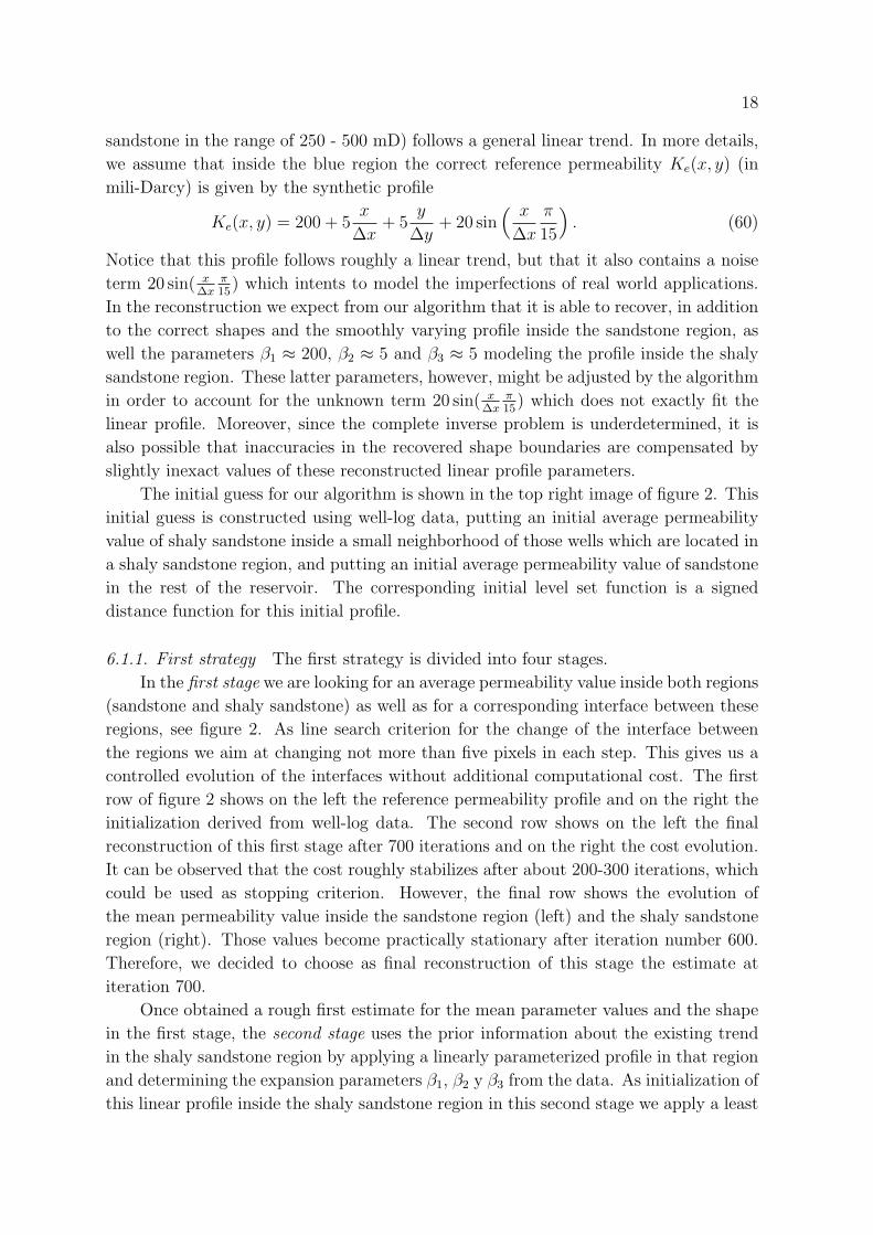
In the top left image of figure 2 we present the reference model of our hybrid

reservoir. The permeability in the yellow/red region (assumed to be sandstone in

the range of 900 - 1300 mili-Darcy (mD)) does not follow any specifically defined

parameterized form, whereas the permeability in the blue region (assumed to be shaly

18

sandstone in the range of 250 - 500 mD) follows a general linear trend. In more details,

we assume that inside the blue region the correct reference permeability Ke(x, y) (in

mili-Darcy) is given by the synthetic profile

Ke(x, y) = 200 + 5x

∆x+ 5

y

∆y+ 20 sin

( x

∆x

π

15

). (60)

Notice that this profile follows roughly a linear trend, but that it also contains a noise

term 20 sin( x∆x

π15

) which intents to model the imperfections of real world applications.

In the reconstruction we expect from our algorithm that it is able to recover, in addition

to the correct shapes and the smoothly varying profile inside the sandstone region, as

well the parameters β1 ≈ 200, β2 ≈ 5 and β3 ≈ 5 modeling the profile inside the shaly

sandstone region. These latter parameters, however, might be adjusted by the algorithm

in order to account for the unknown term 20 sin( x∆x

π15

) which does not exactly fit the

linear profile. Moreover, since the complete inverse problem is underdetermined, it is

also possible that inaccuracies in the recovered shape boundaries are compensated by

slightly inexact values of these reconstructed linear profile parameters.

The initial guess for our algorithm is shown in the top right image of figure 2. This

initial guess is constructed using well-log data, putting an initial average permeability

value of shaly sandstone inside a small neighborhood of those wells which are located in

a shaly sandstone region, and putting an initial average permeability value of sandstone

in the rest of the reservoir. The corresponding initial level set function is a signed

distance function for this initial profile.

6.1.1. First strategy The first strategy is divided into four stages.

In the first stage we are looking for an average permeability value inside both regions

(sandstone and shaly sandstone) as well as for a corresponding interface between these

regions, see figure 2. As line search criterion for the change of the interface between

the regions we aim at changing not more than five pixels in each step. This gives us a

controlled evolution of the interfaces without additional computational cost. The first

row of figure 2 shows on the left the reference permeability profile and on the right the

initialization derived from well-log data. The second row shows on the left the final

reconstruction of this first stage after 700 iterations and on the right the cost evolution.

It can be observed that the cost roughly stabilizes after about 200-300 iterations, which

could be used as stopping criterion. However, the final row shows the evolution of

the mean permeability value inside the sandstone region (left) and the shaly sandstone

region (right). Those values become practically stationary after iteration number 600.

Therefore, we decided to choose as final reconstruction of this stage the estimate at

iteration 700.

Once obtained a rough first estimate for the mean parameter values and the shape

in the first stage, the second stage uses the prior information about the existing trend

in the shaly sandstone region by applying a linearly parameterized profile in that region

and determining the expansion parameters β1, β2 y β3 from the data. As initialization of

this linear profile inside the shaly sandstone region in this second stage we apply a least

19

P1

P2

P3

P4P5P6

P7

P8 P9

I1

I2I3

I4

0 100 200 300 400 500 600

0

100

200

300

400

500

600

300

400

500

600

700

800

900

1000

1100

0 100 200 300 400 500 600

0

100

200

300

400

500

600

300

400

500

600

700

800

900

1000

1100

0 100 200 300 400 500 600

0

100

200

300

400

500

600

300

400

500

600

700

800

900

1000

1100

0 100 200 300 400 500 600 7000.5

1

1.5

2

2.5

3

3.5

0 100 200 300 400 500 600 7001080

1085

1090

1095

1100

1105

1110

1115

1120

0 100 200 300 400 500 600 700290

300

310

320

330

340

350

Figure 2. Hybrid case. First strategy, stage I. Left column from top to bottom:reference permeability, final reconstruction of the first stage, evolution of the meanpermeability value in the sandstone region. Right column from top to bottom:initialization, evolution of cost, evolution of the mean permeability value in theshaly sandstone region. The complete evolution can be seen in the animated fileDVmovie1.gif

squares parameter fitting of β1, β2 and β3 to the well data which correspond to those

wells which are located in the estimated shaly sandstone area of stage I. The remaining

unknowns (the sandstone area and the interface) do not change during this stage. The

evolution of the three parameters and of the cost when minimizing the mismatch to

production data, as well as the final reconstruction of this stage II, can be seen in figure

3.

During the third stage of the algorithm we then focus on the determination of a

smoothly varying profile (pixel-by-pixel updates following the Frechet derivative) inside

the sandstone region which minimizes the mismatch to the production data. Here we

keep the reconstructed linear profile inside the shaly sandstone region and the interface

constant. The evolution of the cost and the final reconstruction (after 700 iterations) of

this third stage can be seen in figure 4. For more details on the pixel-based reconstruction

scheme which is applied here inside the sandstone region we refer to the previous work in

[11] where it has been used as a stand-alone tool for characterizing petroleum reservoirs

20

0 100 200 300 400 500 600

0

100

200

300

400

500

600

300

400

500

600

700

800

900

1000

1100

0 100 200 300 400 500 600

0

100

200

300

400

500

600

300

400

500

600

700

800

900

1000

1100

0 100 200 300 400 500 600 7001

1.5

2

2.5

3

3.5

4

4.5

5

0 100 200 300 400 500 600 700200

210

220

230

240

250

260

270

0 100 200 300 400 500 600 7000.55

0.6

0.65

0.7

0.75

0.8

0.85

0.9

Figure 3. Hybrid case. First strategy, stage II. Top left: final reconstruction of stageII. Top right: initialization of stage II. Bottom left: evolution of the parameters β1,β2, β3. Bottom right: evolution of cost. The complete evolution can be seen in theanimated file DVmovie1.gif

0 100 200 300 400 500 600

0

100

200

300

400

500

600

300

400

500

600

700

800

900

1000

1100

0 100 200 300 400 500 600 7000.53

0.535

0.54

0.545

0.55

0.555

0.56

0.565

0.57

0.575

0.58

Figure 4. Hybrid case. First strategy, stage III. Left: final reconstruction of stageIII. Right: evolution of cost. The complete evolution can be seen in the animated fileDVmovie1.gif

from production data.

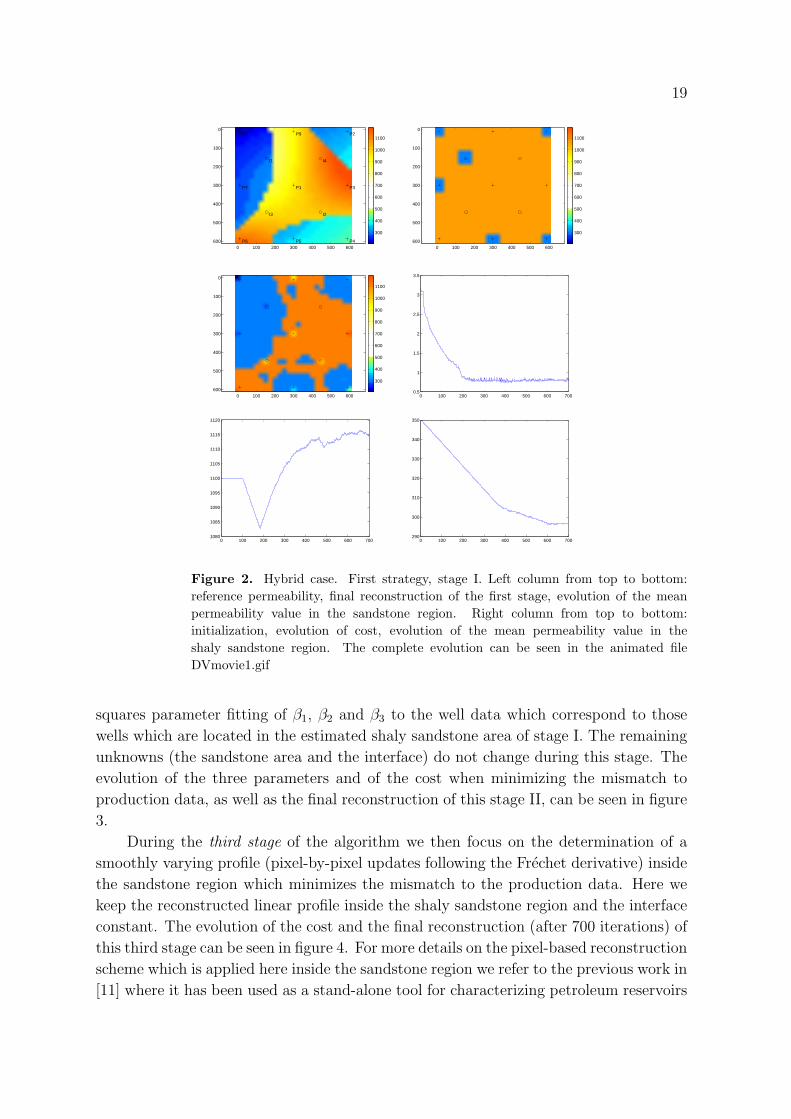
In the fourth stage of the inversion algorithm, all parameters of the inversion

problem (i.e. the level set function, the three parameters inside the shaly sandstone

region and the smoothly varying profile inside the sandstone region) are updated

simultaneously in order to find a joint optimal solution which minimizes the given cost

functional. Figure 5 shows on the top left the reference profile, on the top right the

final reconstruction of stage III which is at the same time the initialization of this stage

IV, on the bottom left the final reconstruction of stage IV, and on the bottom right the

evolution of the cost during this last stage of the algorithm.

21

P1

P2

P3

P4P5P6

P7

P8 P9

I1

I2I3

I4

0 100 200 300 400 500 600

0

100

200

300

400

500

600

300

400

500

600

700

800

900

1000

1100

0 100 200 300 400 500 600

0

100

200

300

400

500

600

300

400

500

600

700

800

900

1000

1100

0 100 200 300 400 500 600

0

100

200

300

400

500

600

300

400

500

600

700

800

900

1000

1100

0 50 100 150 200 2500.35

0.4

0.45

0.5

0.55

0.6

0.65

0.7

Figure 5. Hybrid case. First strategy, stage IV. Top left: reference permeability.Top right: initialization of stage IV. Bottom left: final reconstruction of stage IV.Bottom right: evolution of cost. The complete evolution can be seen in the animatedfile DVmovie1.gif

6.1.2. Second strategy In this second strategy, all unknowns of the inversion problem

are evolved simultaneously from the first iteration to the end of the evolution until the

cost is minimized. In other words, compared to the previously explained first strategy,

we skip here the initial three stages and start immediately with stage IV of that scheme

using as initial guess the profile obtained from well-log data (see the top right image

of figure 6, where in addition the least squares fit of the linear profile parameters to

the permeability data measured at the well locations will be applied in the ’blue region’

before starting the evolution). Certainly, this strategy is the more elegant approach for

solving the inversion problem at hand. However, we mention that the application of

simultaneous updates for all unknowns of this complex inversion problem right from the

beginning requires a very careful calibration of the individual step-sizes with respect

to each other. Otherwise it might result in an unstable or suboptimal evolution of the

different unknowns. This risk is reduced in the previously demonstrated strategy of

applying different stages of increasing complexity for the inversion.

In more details, in this second stage the reconstruction algorithm applies in each

step the following updates simultaneously from just one forward and adjoint calculation:

(i) the update for the level set function using formulas (24), (31), (35); (ii) the update

for the internal permeability profile in the sandstone region which is done pixel by pixel

using formulas (25), (29); (iii) the update for the three parameters β1, β2 and β3 of the

parameterized profile inside the shaly sandstone area using expressions (38), (42).

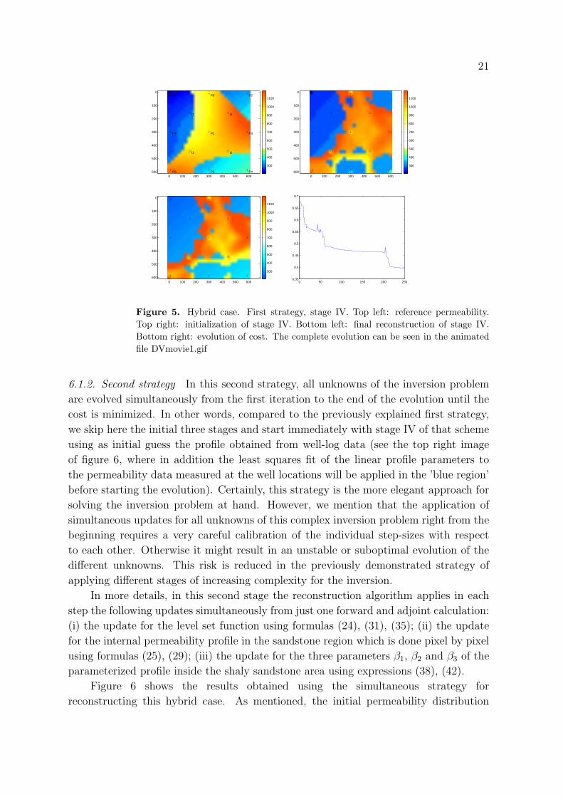
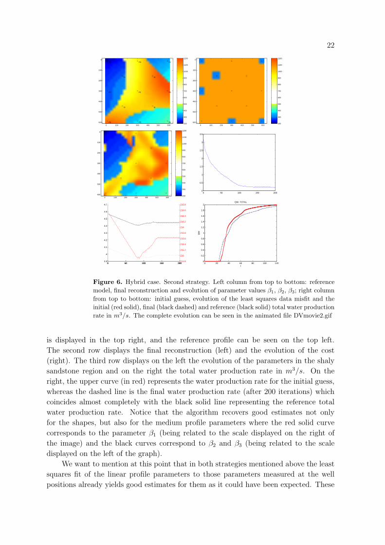
Figure 6 shows the results obtained using the simultaneous strategy for

reconstructing this hybrid case. As mentioned, the initial permeability distribution

22

P1

P2

P3

P4P5P6

P7

P8 P9

I1

I2I3

I4

0 100 200 300 400 500 600

0

100

200

300

400

500

600200

300

400

500

600

700

800

900

1000

1100

1200

0 100 200 300 400 500 600

0

100

200

300

400

500

600200

300

400

500

600

700

800

900

1000

1100

1200

0 100 200 300 400 500 600

0

100

200

300

400

500

600200

300

400

500

600

700

800

900

1000

1100

1200

0 50 100 150 2000

0.5

1

1.5

2

2.5

3

3.5

0 50 100 150 2003.9

4

4.1

4.2

4.3

4.4

4.5

4.6

4.7

0 50 100 150 200214.8

215

215.2

215.4

215.6

215.8

216

216.2

216.4

216.6

216.8

0 20 40 60 80 100 1200

0.2

0.4

0.6

0.8

1

1.2

1.4

1.6

1.8

2QW. TOTAL

t

QW

Figure 6. Hybrid case. Second strategy. Left column from top to bottom: referencemodel, final reconstruction and evolution of parameter values β1, β2, β3; right columnfrom top to bottom: initial guess, evolution of the least squares data misfit and theinitial (red solid), final (black dashed) and reference (black solid) total water productionrate in m3/s. The complete evolution can be seen in the animated file DVmovie2.gif

is displayed in the top right, and the reference profile can be seen on the top left.

The second row displays the final reconstruction (left) and the evolution of the cost

(right). The third row displays on the left the evolution of the parameters in the shaly

sandstone region and on the right the total water production rate in m3/s. On the

right, the upper curve (in red) represents the water production rate for the initial guess,

whereas the dashed line is the final water production rate (after 200 iterations) which

coincides almost completely with the black solid line representing the reference total

water production rate. Notice that the algorithm recovers good estimates not only

for the shapes, but also for the medium profile parameters where the red solid curve

corresponds to the parameter β1 (being related to the scale displayed on the right of

the image) and the black curves correspond to β2 and β3 (being related to the scale

displayed on the left of the graph).

We want to mention at this point that in both strategies mentioned above the least

squares fit of the linear profile parameters to those parameters measured at the well

positions already yields good estimates for them as it could have been expected. These

23

P1

P2

P3

P4P5P6

P7

P8 P9

I1

I2I3

I4

0 100 200 300 400 500 600

0

100

200

300

400

500

600

400

600

800

1000

1200

1400

1600

1800

0 100 200 300 400 500 600

0

100

200

300

400

500

600

400

600

800

1000

1200

1400

1600

1800

0 100 200 300 400 500 600

0

100

200

300

400

500

600

400

600

800

1000

1200

1400

1600

1800

0 50 100 150 200 250 300 350 4000

1

2

3

4

5

6

7

8

9

0 100 200 300 400 500 600

0

100

200

300

400

500

600

400

600

800

1000

1200

1400

1600

1800

0 100 200 300 400 500 6001

2

3

4

5

6

7

8

9

10

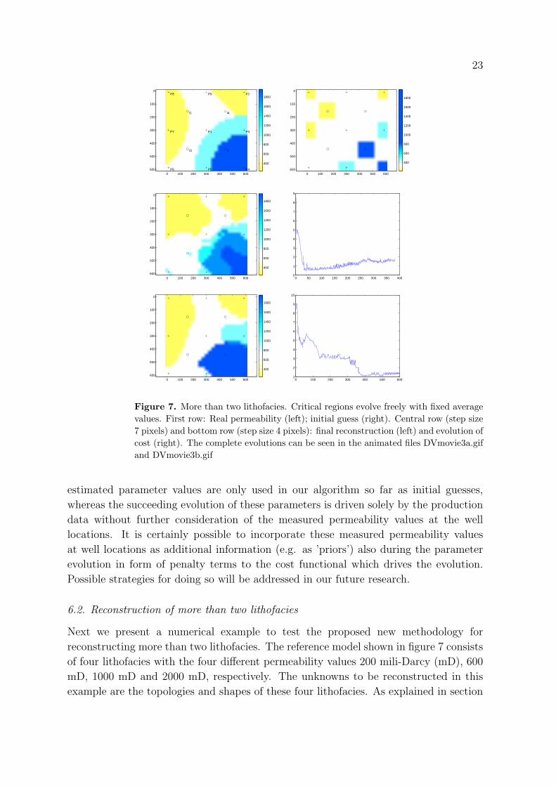
Figure 7. More than two lithofacies. Critical regions evolve freely with fixed averagevalues. First row: Real permeability (left); initial guess (right). Central row (step size7 pixels) and bottom row (step size 4 pixels): final reconstruction (left) and evolution ofcost (right). The complete evolutions can be seen in the animated files DVmovie3a.gifand DVmovie3b.gif

estimated parameter values are only used in our algorithm so far as initial guesses,

whereas the succeeding evolution of these parameters is driven solely by the production

data without further consideration of the measured permeability values at the well

locations. It is certainly possible to incorporate these measured permeability values

at well locations as additional information (e.g. as ’priors’) also during the parameter

evolution in form of penalty terms to the cost functional which drives the evolution.

Possible strategies for doing so will be addressed in our future research.

6.2. Reconstruction of more than two lithofacies

Next we present a numerical example to test the proposed new methodology for

reconstructing more than two lithofacies. The reference model shown in figure 7 consists

of four lithofacies with the four different permeability values 200 mili-Darcy (mD), 600

mD, 1000 mD and 2000 mD, respectively. The unknowns to be reconstructed in this

example are the topologies and shapes of these four lithofacies. As explained in section

24

4 the idea is now to evolve three level set functions simultaneously.

Shape evolution without extra treatment of critical regions.

First we investigate the performance of the algorithm as explained in section 4

by letting the critical regions evolve freely and allowing for final reconstructions which

include these critical regions as ’regions of uncertainty’.

We initialize the evolution using the permeability values at the well locations and

applying them in a small neighbourhood of these well locations. The background value

is the value which appears more than the others at the well locations (in this case 600

mD). See the top right image of the figure 7. The top left image of this figure shows the

corresponding reference permeability profile. The first strategy consist of evolving the

initial level set function from the initial guess without eliminating the critical regions

using different step sizes. In the second and third rows of figure 7 are displayed the

results obtained applying two different step size criteria for the level set function during

the evolution process. The first step size criterion (second row) changes maximally 7

pixel values in each step of the evolution, whereas the second step size criterion (bottom

row) allows for not more than 4 pixels to change value in each step. On the right hand

side of the rows two and three, the evolution of the cost for these two step size criteria

is shown. We observe that the change of 7 pixel values represents already quite a large

step-size such that the cost is reduced significantly during the first iterations until it

reaches a low value, but then it starts increasing slightly since large steps are inforced

also at later iterations. Reducing the step size to the change of only 4 pixels restores the

descent property of the evolution but decreases the cost at a slower rate. We mention

that, additionally, during the evolution in the latter case (4 pixels changing) the level

set functions are rescaled in each step such that their minimum values remain constant

inside the domain which might have a small effect as well on the evolution. Which of

the final reconstructions actually is the ’better’ or ’more useful’ one is difficult to say in

this case.

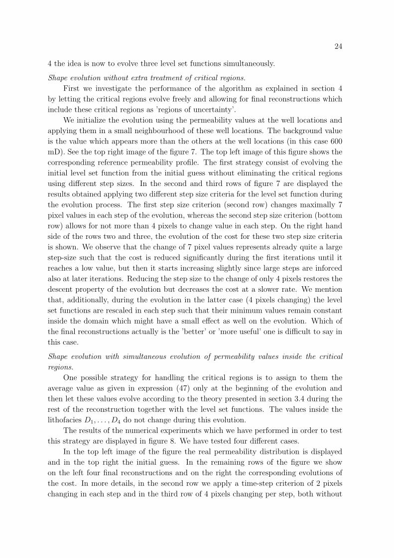
Shape evolution with simultaneous evolution of permeability values inside the critical

regions.

One possible strategy for handling the critical regions is to assign to them the

average value as given in expression (47) only at the beginning of the evolution and

then let these values evolve according to the theory presented in section 3.4 during the

rest of the reconstruction together with the level set functions. The values inside the

lithofacies D1, . . . , D4 do not change during this evolution.

The results of the numerical experiments which we have performed in order to test

this strategy are displayed in figure 8. We have tested four different cases.

In the top left image of the figure the real permeability distribution is displayed

and in the top right the initial guess. In the remaining rows of the figure we show

on the left four final reconstructions and on the right the corresponding evolutions of

the cost. In more details, in the second row we apply a time-step criterion of 2 pixels

changing in each step and in the third row of 4 pixels changing per step, both without

25

P1

P2

P3

P4P5P6

P7

P8 P9

I1

I2I3

I4

0 100 200 300 400 500 600

0

100

200

300

400

500

600

400

600

800

1000

1200

1400

1600

1800

0 100 200 300 400 500 600

0

100

200

300

400

500

600

400

600

800

1000

1200

1400

1600

1800

0 100 200 300 400 500 600

0

100

200

300

400

500

600

400

600

800

1000

1200

1400

1600

1800

0 50 100 150 200 250 300 3501

2

3

4

5

6

7

8

9

10

11

0 100 200 300 400 500 600

0

100

200

300

400

500

600

400

600

800

1000

1200

1400

1600

1800

0 200 400 600 800 10000

2

4

6

8

10

12

14

16

0 100 200 300 400 500 600

0

100

200

300

400

500

600

400

600

800

1000

1200

1400

1600

1800

0 50 100 150 200 250 300 3500

1

2

3

4

5

6

7

8

9

0 100 200 300 400 500 600

0

100

200

300

400

500

600

400

600

800

1000

1200

1400

1600

1800

0 100 200 300 400 500 600 700 8000

1

2

3

4

5

6

7

8

9

Figure 8. More than two lithofacies. Values inside critical regions are corrected ineach step. First row: real permeability (left); initial guess (right). Rows two to five:final reconstruction on the left and evolution of cost on the right for several differentcases. Row two: step size 2 without rescaling of level set function. Row three: step size4 without rescaling. Row four: step size 2 with rescaling. Row five: step size 4 withrescaling. The complete evolutions can be seen in the animated files DVmovie4a.gif-DVmovie4d.gif

26

P1

P2

P3

P4P5P6

P7

P8 P9

I1

I2I3

I4

0 100 200 300 400 500 600

0

100

200

300

400

500

600

400

600

800

1000

1200

1400

1600

1800

0 100 200 300 400 500 600

0

100

200

300

400

500

600 200

400

600

800

1000

1200

1400

1600

1800

2000

0 100 200 300 400 500 600

0

100

200

300

400

500

600

400

600

800

1000

1200

1400

1600

1800

0 100 200 300 400 500 600 700 8000

1

2

3

4

5

6

7

8

9

10

Figure 9. More than two lithofacies. Values inside critical regions are corrected ineach step and penalization of critical region is applied. First row: Real permeability(left); initial guess (right). Second row: final reconstruction (left) and evolution of cost(right). The complete evolution can be seen in the animated file DVmovie5.gif

re-scaling of the level set function. In rows four and five we show the corresponding

results (in the same order as before) with re-scaling (the minimum is fixed to a value

of −200) of the level set function in each step. It can be seen that the critical regions

are reduced in all cases, but that the corresponding evolutions lead to slightly different

reconstructions (which we might interpret as different ’local minima’). This is probably

due to the severe ill-posedness of the problem and the sparsity of the data.

Shape evolution with additional penalization of area of critical regions.

This final example is chosen for showing how the penalty technique described in

the expressions (55) and (56) performs for the elimination of critical regions during the

evolution of more than one level set function. Notice that also the ’true reservoir’ has

been chosen here slightly different from the previous one. Compared to the previous

example three wells are now situated in a different region such that they yield different

well-logs and therefore the initial guess has changed.

In figure 9 we display the results obtained by applying this additional regularization

technique. As before, on the top left the real permeability distribution is displayed and

on the top right we show the initial guess. On the bottom the final reconstruction

obtained by this technique (left) and the evolution of the cost (right) are displayed.

Also here the criticial region is practically removed in the final reconstruction and the

overall reconstruction is satisfactory, even though some parts of the reservoir (with

smaller sensitivity to the data) could not be characterized correctly. Again, this is

probably due to the sparsity of the data and the ill-posedness of the inverse problem.

27

6.3. Reconstruction of channel or barrier structures

Here we present numerical examples for our strategy for testing the existence of certain

geometrical shapes in the reservoir based on topological perturbations (see section 5).

For simplicity we concentrate here on a reservoir which is assumed to have a piecewise

constant permeability profile with unknown values. The goal of the algorithm is to

recover the topology and shapes of the regions together with their correct permeability

values. For this purpose, we apply the shape evolution algorithm based on level sets

and the evolution of constant permeability values (as described in subsection 3.4)

simultaneously until the algorithm converges. The result of this strategy is displayed

in figure 10. In the first row of the figure the real or reference model (left) and the

initial guess (right) based on well information are shown. The second row shows the

final reconstruction (left) and the corresponding evolution of the cost (right). In the

third row we show the evolution of the estimated permeability values in the sandstone

(left) and shaly sandstone (right) region.

As it can be seen in the final reconstruction, the barrier which is present in the

reservoir has not been recovered completely. The reservoir engineer might have some

idea about the existence of a barrier in the reservoir and might therefore want to test if in

fact the barrier can be confirmed by the production data and, if it exists, determine some

of the geometrical properties (orientation, width, length) of the barrier. For this purpose,

our algorithm provides the opportunity to add a barrier of arbitrary length, width and

orientation to the reservoir at the location where the reservoir engineer assumes that it

should be located. Practically the technique explained in section 5 is applied at some

step of the algorithm for perturbing the current level set function such that the barrier

is introduced. Then, the level set function continues its evolution starting out from the

perturbed guess. The idea is that the added barrier will evolve and deform in the intent

to satisfy the data. It might either change orientation, or disappear or just adjust its

boundaries depending on the correctness of the assumptions which are incorporated in

the added barrier. We mention at this point that a similar strategy has been applied

in our previous work in order to handle objects hidden in areas of low sensitivity (for

details see [34]).

The first numerical experiment tests the ideal situation where the guess of the

reservoir engineer is correct and the seed barrier is put at the correct location with

the correct orientation. Figure 11 shows the results in this case. On the top left the

reference profile is shown, on the top right the initial guess (which is the final result of

figure 10), on the bottom left the final reconstruction of this additional step, and on the

bottom right the evolution of the cost during these additional iterations after adding the

test barrier. Obviously, adding a test barrier with the correct location and orientation

opens the way for the algorithm to arrive at an improved reconstruction. Notice that

the final cost after this additional evolution is not significantly lower than the final cost

of the previous step shown in figure 10. We interpret this fact by saying that adding

the guess for the barrier helped us to get out of one (local) minimum and arriving at

28

P1

P2

P3

P4P5P6

P7

P8 P9

I1

I2I3

I4

0 100 200 300 400 500 600

0

100

200

300

400

500

600

400

600

800

1000

1200

1400

0 100 200 300 400 500 600

0

100

200

300

400

500

600

400

600

800

1000

1200

1400

0 100 200 300 400 500 600

0

100

200

300

400

500

600

400

600

800

1000

1200

1400

0 500 1000 15000

1

2

3

4

5

6

7

8

0 500 1000 15001250

1300

1350

1400

1450

1500

1550

0 500 1000 1500250

255

260

265

270

275

280

285

290

295

300

Figure 10. Barriers, first stage. Shape and mean value reconstruction foreach lithofacie. Reference permeability (top left); initial guess (top right); finalreconstruction (central left); evolution of the cost functional (central right); evolution ofthe mean sandstone permeability value (bottom left) and of the mean shaly sandstonepermeability value (bottom right). The complete evolution can be seen in the animatedfile DVmovie6.gif

another (local) minimum of the cost functional.

In order to further test the algorithm (and the non-uniqueness of the underlying

inverse problem), we have done a second numerical experiment where we add a seed

barrier which has, in contrary to the reference barrier with a 45o inclination, a horizontal

orientation. The results are shown in figure 12, with the same arrangement of images

as before. Surprisingly, it can be observed that the horizontal barrier persists and, even

worse, the cost value of the final reconstruction (showing a horizontal barrier) is lower

than the final cost values of the previous two reconstructions. Also here we explain

the result by the sparsity of the available production data and the ill-posedness of the

inverse problem. The noise in the data can easily change the solution in regions of low

sensitivity since the effect of these changes to the data is at the noise level.

29

P1

P2

P3

P4P5P6

P7

P8 P9

I1

I2I3

I4

0 100 200 300 400 500 600

0

100

200

300

400

500

600

400

600

800

1000

1200

1400

0 100 200 300 400 500 600

0

100

200

300

400

500

600

400

600

800

1000

1200

1400

0 100 200 300 400 500 600

0

100

200

300

400

500

600

400

600

800

1000

1200

1400

0 200 400 600 800 1000 1200

0.8

1

1.2

1.4

1.6

1.8

2

Figure 11. Barriers, second stage: first numerical experiment. Top row: Realpermeability (left); initial guess (right). Bottom row: Final reconstruction after addingan inclined barrier and evolving the shape (left); evolution of the cost functional inthis second stage (right). The complete evolution can be seen in the animated fileDVmovie7.gif

P1

P2

P3

P4P5P6

P7

P8 P9

I1

I2I3

I4

0 100 200 300 400 500 600

0

100

200

300

400

500

600

400

600

800

1000

1200

1400

0 100 200 300 400 500 600

0

100

200

300

400

500

600

400

600

800

1000

1200

1400

0 100 200 300 400 500 600

0

100

200

300

400

500

600

400

600

800

1000

1200

1400

0 200 400 600 800 1000 1200 1400

0.8

1

1.2

1.4

1.6

1.8

2

2.2

2.4

2.6

Figure 12. Barriers, second stage: second numerical experiment. As in figure 11,but after adding a horizontal seed barrier. The complete evolution can be seen in theanimated file DVmovie8.gif

30

7. Conclusions

We have introduced in this paper a new reconstruction scheme for the history matching

problem of reservoirs with an arbitrary number of lithofacies using a level set technique.

In each of the lithofacies a smoothly varying permeability profile (either pixel-by-pixel or

parameterized) can be assumed and is reconstructed as well from the data. In this sense,

our new algorithm is a generalization of classical reservoir characterization algorithms

which do not incorporate sharp interfaces between lithofacies in the reservoir (which in

our algorithm amounts to the special case where we assume that the entire reservoir

contains only one region). Our numerical experiments have addressed the situation of

reservoirs with two lithofacies and a hybrid arrangement of internal permeability profiles

as well as reservoirs with more than two (here four) lithofacies assuming piecewise

constant permeability profiles. The numerical results from synthetically created data

(using a simulator completely independent from the simulator used in the reconstruction

process and adding a sufficient amount of modelling and data noise) for realistic

situations convince us that the algorithm provides very good estimates of structured

reservoirs. In addition, we have tested here the use of topological perturbations for

verifying the existence of certain geometrical objects (such as channels or barriers) in the

reservoir. We believe that any combination of these basic building blocks can be applied

without problems for characterizing real reservoirs and that, putting them all together,

will provide the reservoir engineer with a powerful alternative reservoir characterization

tool with very attractive additional features compared to the already existing classical

tools. The algorithm can be extended easily to more realistic 3D situations as long

as reservoir simulators for the forward and the adjoint problem are available. These

simulators can be integrated in the reconstruction algorithm as black box solvers, such

that the favourite tool of the reservoir engineer for simulating a given reservoir can be

applied without problems during the characterization process.

Acknowledgments

Funding for this work was provided by the Direccion de Tecnologıa y Soporte Tecnico,

Repsol-YPF.

References

[1] Agarwal B and Blunt M 2003 A streamline-based method for assisted history matching applied toan Arabian Gulf field, SPE paper 84462, SPE ATCE, Denver, CO, Oct. 5–8.

[2] Berre I, Lien M and Mannseth T 2007 A level set corrector to an adaptive multiscale permeabilityprediction, Computational Geosciences 11 (1) 27–42.

[3] Carter R D, Kemp Jr L F, Pierce A C and Williams D L 1974 Performance Matching WithConstraints SPE Journal 14 187–196.

[4] Chan T F and Tai X-C 2003 Level set and total variation regularization for elliptic inverse problemswith discontinuous coefficients J. Comput. Physics 193 40–66.

31

[5] Chavent G, Dupuy M and Lemmonier C 1975 History Matching by Use of Optimal Control TheorySPE Journal 15 74-86.

[6] Crichlow H B 1976 Modern Reservoir Engineering-A Simulation Approach, Prentice Hall, NewJersey.

[7] Deutsch C V and Journel A G, GSLIB: Geostatistical Software Library and User’s Guide, AppliedGeostatistics Series, Oxford University Press, 1997

[8] Dorn O and Lesselier D, 2006. Level set methods for inverse scattering. Topical Review. InverseProblems 22 R67-R131.

[9] Dorn O, Miller E L and Rappaport C 2000, A shape reconstruction method for electromagnetictomography using adoint fields and level sets, Inverse Problems 16, 1119–1156.

[10] Ewing R E, Pilant M S, Wade J G and Watson A T 1995 Identification and Control Problemsin Petroleum and Groundwater Modeling, Control Problems in Industry (I. Lasciecka and B.Morton, eds.), Progress in Systems and Control Theory, Birkhauser, 119-149.

[11] Gonzalez-Rodriguez P, Kindelan M, Moscoso M and Dorn O 2005 History matching problem inreservoir engineering using the propagation back-propagation method Inverse Problems 21, 565-590.

[12] Gu Y, and Oliver D S 2004 History matching of the PUNQ- S3 reservoir model: Using the ensembleKalman filter, In SPE Annual Technical Conference and Exhibition, Houston, Texas, 26-29September 2004 (Society of Petroleum Engineers SPE 90962).

[13] Jacquard P and Jain C 1965 Permeability Distribution From Field Pressure Data SPE Journal 5281-294.

[14] Li R, Reynolds A C and Oliver D S 2003 History matching of three-phase flow production data,SPE Journal 8 328-340.

[15] Lie J, Lysaker M, and Tai X 2006 A variant of the level set method and applications to imagesegmentation. Mathematics of Computation 75 1155–1174.

[16] Lien M, Mannseth T 2006 Resolution power of pressure data for permeability identificationTransport in Porous Media 64 (2) 141–159.

[17] Lien M, Jansen J D, Mannseth T, Brouwer R 2005 Multiscale Regularization of Dynamic WaterFlood Optimization. Submitted to Computational Geosciences.

[18] Lien M, Berre I, and Mannseth T 2006 Combined adaptive multiscale and level set parameterestimation. Proceedings: The Third International Conference ’Inverse Problems: Modeling andSimulation’ May 29-June 02, Fethiye, Turkey, 2006

[19] Litman A 2005 Reconstruction by level sets of n-ary scattering obstacles Inverse Problems 21S131–S152.

[20] Liu N, and Oliver D S 2005 Ensemble Kalman filter for automatic history matching of geologicfacies Journal of Petroleum Science and Engineering 47 (3-4) 147-161.

[21] Osher S and Shetian J 1988 Fronts propagation with curvature dependent speed: algorithms basedon Hamilton-Jacobi formulations J. Comput. Physics 56 12–49.

[22] Osher S and Fedkiw R Level set methods and dynamic implicit surfaces, Springer, New York, 2003.[23] Rahon D, Blanc G, and Guerillot D 1996 Three-Dimensional Reservoir description from multiwell

Pressure Data and Prior information Society of Petroleum Engineers SPE-paper 36509.[24] Rahon D et al 1998 Identification of geological shapes in reservoir engineering by history matching

production data Society of Petroleum Engineers SPE-paper 48969.[25] Santosa F 1996 A level-set approach for inverse problems involving obstacles, ESAIM: Control,

Optimization and Calculus of Variations 1, 17–22.[26] Sethian J A, Level Set Methods and Fast Marching Methods, (2nd ed) Cambridge University Press,

1999.[27] Sun N and Yeh W G 1990 Coupled inverse problems in groundwater modelling 1. Sensitivity

analysis and parameter identification Water resources research 26 2507-2525.[28] Tai X-C, and Yao C 2005 Fast Piecewise Constant Level Set Methods (PCLSM) with Newton

Updating CAM-report, CAM-05-51 UCLA.

32

[29] Thomas G W 1982 Principles of Hydrocarbon Reservoir Simulation, Prentice-Hall.[30] Vasco D M Yoon S and Datta-Gupta A 1999 Integrating Dynamic Data Into High-Resolution

Reservoir Models Using Streamline-Based Analytic Sensitivity Coefficients Society of PetroleumEngineers SPE Journal 4 389-399.

[31] Villegas R, Dorn O, Moscoso M and Kindelan M 2006 Shape reconstruction from two-phaseincompressible flow data using level sets Proc. International conference on PDE-based imageprocessing and related inverse problems, CMA, Oslo: August 2005 (Eds: X.-C. Tai, K.-A. Lie,T.F. Chan, and S. Osher), pp. 381-401, Series: Mathematics and Visualization, Publisher:Springer ISBN 078-3-540-33266-4 .

[32] Villegas R, Dorn O, Moscoso M, Kindelan M and Mustieles F J 2006 Simultaneous characterizationof geological shapes and permeability distributions in reservoirs using the level set method Proc.SPE Europec/EAGE Annual Conference and Exhibition, Vienna: June 2006 (Proc. paper C015)(Society of Petroleum Engineers SPE-paper 1002911) 1–12.

[33] Villegas R, Dorn O, Moscoso M and Kindelan M 2006 Simultaneous characterization of geologicalregions and parameterized internal permeability profiles in history matching, Proc. 10thEuropean conference on the mathematics of oil recovery ECMOR X, 4-7 Sept., Amsterdam,Netherlands, Proc. paper A015.

[34] Villegas R, Dorn O, Kindelan M and Moscoso M 2007 Imaging low sensitivity regions inpetroleum reservoirs using topological perturbations and level sets Journal of Inverse and Ill-posed Problems, 15 (2) 199-223.

[35] Villegas R, Dorn O, Moscoso M and Kindelan M 2007 Characterization of reservoirs by evolvinglevel set functions obtained from geostatistics Proc. 14th European Conference on Mathematicsfor Industry (ECMI 2006),10-14 July 2006, Leganes, Spain (Publisher: Springer) (to appear)