February 1, 2001

Historic Shoreline Change at Lake Tahoe From 1938 to 1998: Implications for Water Clarity

Report Submitted to:

Tahoe Regional Planning Agency

Submitted by:

Kenneth D. Adams Timothy B. Minor

Desert Research Institute

University and Community College System of Nevada

Desert Research Institute

February 1, 2001 1

Historic Shoreline Change at Lake Tahoe From 1938 to 1998: Implications for Water Clarity

Final Report Submitted on

February 1, 2001

Kenneth D. Adams Timothy B. Minor

Desert Research Institute EXECUTIVE SUMMARY The goal of this study was to estimate the contribution of sediment and nutrient loading into Lake Tahoe from shoreline erosion. To accomplish this goal we first incorporated georectified aerial photographs from 1938 to the present into an ArcView GIS database to track shoreline changes over the last 60 years. This phase of the study was augmented by more detailed field studies and collection of sediment samples for nutrient analyses. Approximately 80 samples were collected and analyzed at DRI for phosphorus and nitrogen content. Using the GIS database, surface areas of both eroding and accreting shorezones were calculated. For segments undergoing erosion, the areas were converted to volumetric estimates by estimating their thickness from 1918-1919 U.S. Bureau of Reclamation topographic maps with 1 and 5 foot contour intervals. Approximately 429,000 metric tons (MT) of sediment has been eroded into the lake from shorezone sources since 1938. Using the nutrient concentrations from this study, approximately 117 MT of phosphorus and 110 MT of nitrogen have also been washed into the lake during the same time period. These values equate to about 2 MT per year of phosphorus and about 1.8 MT per year of nitrogen and are considered to be accurate within a factor of two. Although these values are still relatively small compared to other sources of these nutrients, it must be borne in mind that their relative contribution will increase if some of the other sources have been overestimated. INTRODUCTION Lake Tahoe is known for its beauty and crystal clear waters. However, the lake has been decreasing in clarity at the rate of about 0.3 m per year since about 1968 (Jassby et al., 1999). The primary causes for this decrease are thought to be the introduction of sediment and nutrients, primarily phosphorus and nitrogen, into the Lake. Five sources of these nutrients have been identified that include atmospheric deposition, stream loading, direct runoff, groundwater, and shorezone erosion (Working Draft of the Lake Tahoe Watershed Assessment-LTWA). The goals of this study are to delineate the mass of sediment and nutrients introduced into Lake Tahoe over the last 60 years from shoreline erosion and to compare these values to the other identified sources. The shorezone surrounding oligotrophic Lake Tahoe is a very dynamic environment where sediment is eroded, transported, and deposited on an annual basis. Waves in the nearshore area also help to redistribute sediment delivered to the Lake by inflowing streams. However, the extent of shoreline erosion, littoral sediment movement, and its effect on the water quality of Lake Tahoe is relatively unknown. Therefore, we have

Desert Research Institute

February 1, 2001 2

performed a detailed study, incorporating georectified historical air photos into a GIS database (see enclosed CD) combined with field observations and nutrient sampling, to determine the amount and processes of phosphorus and nitrogen input into the Lake from shoreline sources. Volumetric estimates derived from this study are then compared to other sources of these nutrients to determine the relative magnitude of nutrient input from the shorezone. The physical setting of Lake Tahoe The geologic history of the Lake Tahoe basin provides an important context for studying the shoreline system of this high elevation lake. In particular, the Quaternary (0 to 2,000,000 years ago) history of the basin can be directly correlated to the material characteristics, processes, and rates of change found on different lengths of shoreline around the lake. Lake levels have naturally fluctuated at Lake Tahoe, depositing nearshore beach and other lacustrine deposits at both higher and lower levels than today. These deposits and their material properties are the ones that need to be considered when studying shoreline change at Lake Tahoe. Therefore, this section provides a brief discussion of the general geology of the Lake Tahoe basin, but focuses on the more recent history when glaciers repeatedly advanced and receded and lake levels rose and fell for reasons that are not as yet entirely understood. This discussion is based on existing literature and from observations made during the course of this study. Lake Tahoe sits astride the crest of the Sierra Nevada in a large tectonic graben still bounded by active faults. This graben is the westernmost expression of Basin and Range extension at this latitude and is bounded on the east side by the Carson Range and on the west by the Sierra Nevada crest (Gardner et al., 2000). Although faults are more difficult to discern on land in the Tahoe basin, apparently young fault scarps traversing the floor of the lake demonstrate that this basin is still tectonically active (Gardner et al., 1999). The vast majority of exposed bedrock in the basin consists of granitic rocks, but the north end is filled with a large pile of Tertiary and Pleistocene volcanic rocks. Scattered metamorphic rocks, particularly around Mt. Tallac, also exist in the basin (Burnett, 1971). The general geology of the basin is shown in figure 1 which portrays the distribution of rocks and sediments in the basin. The geologic map shows a variety of different geologic units near lake level, each of which probably responds to wave action in different ways. Along the east shore of the lake, granitic bedrock dominates except for a few small pocket beaches such as Sand Harbor, Glenbrook Bay, and Zephyr Cove. The southern shore is largely composed of glacial outwash deposits into which young lake deposits are inset (Fig. 1). At the shore, the outwash appears to be graded to levels higher than the current lake level of 1899 m, which means that either there has been significant shore erosion since the outwash was deposited or that the outwash was deposited when lake levels were higher. The west shore of the lake is dominated by glacial moraines, outwash, and lake deposits, although granitic bedrock does crop out near Rubicon Point. The north shore of the lake is largely comprised of volcanic rocks with some granitics around Stateline Point and abundant areas of lake deposits near the shore (Fig. 1).

Desert Research Institute

February 1, 2001 3

Glacial deposits adjacent to the lake generally date from one of three major glacial episodes that include, from oldest to youngest, the Donner Lake, Tahoe, and Tioga glaciations. The Donner Lake glaciation has been difficult to date, but may be as old as 400,000 to 600,000 years (Birkeland, 1964). Till and moraines of Tahoe age have not been directly dated in the basin, but correlative deposits along the east side of the Sierra Nevada near Yosemite date from about 70,000 years ago, 140,000 years ago, or from both times (Bursik and Gillespie, 1993; Phillips et al., 1990). The Tioga glaciation was the last major glaciation and reached its maximum advance around 20,000 years ago. The abundance of lake deposits cropping out near the shore of Lake Tahoe indicates that lake level, at times, has been much higher than the current level of 1899 m. Periodic ice dams just downstream from the lake outlet may be one cause of these higher lake levels. Birkeland (1964) presents evidence that all three of the major glacial episodes may have dammed Lake Tahoe and caused higher than present lake levels. During Donner Lake time, most of the Truckee River Canyon was filled with ice flowing east from the Sierran crest. Lake deposits and benches found to elevations of 2073 m may relate to this damming episode (Birkeland, 1964). In Tahoe time, ice from Squaw Creek blocked the Truckee River and caused Lake Tahoe to rise to about 1926 m before the dam broke. The sudden release of more than 14 cubic kilometers of water caused a catastrophic flood that coursed down the river and eventually ended up in Lake Lahontan. Curiously, Birkeland (1964) thought that ice damming was negligible in Tioga time, even though his mapping clearly shows that Tioga ice blocked the Truckee River to an elevation of about 1902 m, or approximately 5 m above the natural outlet. The volume of water ponded by a dam at 1902 m equates to about 3 cubic kilometers, quite enough for a large flood event. During the mid-Holocene (4,000 to 7,000 years ago), lake level at Tahoe may have fallen below the natural rim for an extended period of time. Lindstrom (1990) presents evidence that rising waters between 4,000 and 5,000 years ago drowned currently submerged trees along the south shore of Tahoe. The implication is that Tahoe did not spill for an extended period of time allowing forests to colonize areas adjacent to the lower lake level. When climate became effectively wetter around 4000 years ago, Lake Tahoe again rose to its rim and drowned these trees. Davis (1976) reviewed the physical evidence for lower lake levels during this same time period. In particular, the major drainages of the upper Truckee River, Trout Creek, and Taylor Creek were graded to base levels much lower than present and deeply dissected into the glacial outwash plains along the south shore. When water level began to rise at the end of the middle Holocene, these drainages were backfilled and beach barriers developed at the lake-marsh interfaces. According to this model, much of the material filling the marshes around Lake Tahoe dates from the last few thousand years. In the early part of the 20th century, lake levels commonly exceeded the now legally mandated maximum elevation of 1896.65 m (6229.1 ft) (Figure 2). The highest historic level was in 1907 when the lake rose above 1899.29 m (6231.19 ft). Shoreline erosion undoubtedly occurred during these high water periods, but the photography used in our study does not extend far enough back in time to capture the effects of these high water periods.

Desert Research Institute

February 1, 2001 4

METHODOLOGY This study combined a GIS analysis using georectified historical aerial photographs with fieldwork consisting of confirming the air photo interpretations, documenting physical conditions along the shore, and collecting samples for nutrient analyses. Each of these efforts is outlined in the following sections. Aerial Photograph Acquisition Historical aerial photographs and mosaicked digital orthophotographic quadrangles (DOQs) spanning 60 years were acquired from the U.S. Geological Survey (USGS), U.S. Forest Service (USFS), and Tahoe Regional Planning Agency (TRPA). Table 1 indicates the dates the photographs were taken, the geographic location, photographic scale, and responsible agency. Photographic scales ranged from 1:8,000 to 1:20,000. A scale of 1:20,000 photography is considered the smallest usable for shoreline mapping (Moore, 2000). The color and black and white photographic prints were scanned and digitized using a flat bed scanner. Scan rates varied between 300 dots per inch (dpi) and 600 dpi, depending on the scale and quality of the photographic prints. Using the scan rate, print dimensions, and digital image dimensions (in picture elements or pixels), the nominal ground resolutions of the aerial photographs were calculated; for the 1:20,000 scale prints, the ground resolution was 2 meters, for the 1:8,000 scale photographs from 1995, the ground resolution was 1 meter. The ground resolution for the two DOQs was also one meter. Image Processing Methods The multi-date, multi-scale aerial photographs of the Lake Tahoe basin were rectified to the one meter DOQs in a standard polynomial based image-to-map rectification process using ENVI image processing software. Initial attempts to orthorectify the historical photographs proved unsuccessful, as the camera parameters required to build interior orientation were not available for the older photographs (fiducial marks and focal length are required to establish the relationship between the camera model, the aerial photos, Ground Control Points (GCPs), and a Digital Elevation Model (DEM)). DRI also attempted to rectify the aerial photographs using a Delaunay triangulation warping method, which fits triangles to irregularly spaced GCPs and interpolates new values. This method was unsuccessful, however, because it required control points on all sides of the feature of interest, in this case the shoreline, and selecting control points in the lake was not possible. The image-to-map rectification process involved the selection of ground control points common to both the scanned aerial photography and the USGS DOQs. Several rule bases were developed for the point selection process in order to minimize potential errors that can accumulate and contribute to inaccurate shoreline interpretation results. Favorable control points selected included anthropogenic and natural features that were distinct and common to both data sets (road intersections, buildings, trees, and near shore boulders). Care was taken to be cognizant of shadowing effects in the photography and DOQs when selecting GCPs, as these sometimes distorted the precise location of a feature. To avoid the introduction of spatial errors due to lens distortion and camera tilt, control points were

Desert Research Institute

February 1, 2001 5

preferentially selected in the center of each unrectified photograph. Along steep shores, control points were only selected near the shorezone to avoid errors related to topographic relief displacement. Selecting control points at elevations significantly higher than lake level introduces significant errors into the rectification process. This was evident when selecting control points on photos taken over the Emerald Bay region; greater errors were observed for points selected at higher elevations along Highway 89 than those located near the shore. A minimum of ten GCPs was selected for each scanned photograph. Older photographs presented greater challenges in the process, as there were often few common features found between the historical aerial photography and the more recent DOQs. Total Root Mean Square (RMS) error, a relative measure of the accuracy of a polynomial fit between the predicted and observed locations of control points in an input image relative to the map (in this case the DOQs), averaged around 2.0-2.25 for each of the photographs rectified. That is, for each of the photo images rectified, the total, averaged RMS for all the control points in that image was approximately 2.1; most of the RMS errors attributed to control points along the immediate shorezone were actually much less, on the order of 1.0. In ground distance, a RMS error of 1.0 for the 1:20,000 scale photographs was 2 meters. For the 1:8,000 scale 1995 photographs, the RMS error ground distance was one meter. Several iterations were often required in the GCP selection process to arrive at a satisfactory RMS level for all the photographs. Once the GCPs were selected, a first-degree polynomial warping algorithm was implemented, with a nearest neighbor resampling method. The uncorrected images were warped and resampled to the DOQs, cast into a UTM zone 10 coordinate system based on the NAD27 datum. Based on the calculated RMS errors observed in the rectification process, the observed spatial error over an entire photograph was +/- four meters; in actuality that error term is much less for the feature of interest, the shorezone, where the error is closer to +/- 2 meters for the 1:20,000 scale photography, and even less for the 1995 imagery. These numbers all exceed the National Mapping Accuracy Standards defined by the USGS in 1941 (10.2 meters for 1:20,000 scale data; 8.0 meters for 1:8,000 scale). Delineating the Shoreline The first challenge in mapping the former position of the shoreline is to define a consistent and obvious shoreline feature, one that can be recognized on multiple generations of aerial photographs of varying quality. The line between wet sediment and dry sediment is the most commonly used proxy for shoreline position because it approximates the mean high water line (Dolan et al., 1980; Moore, 2000). However, most studies using this proxy have been conducted on open marine coasts, where the lateral position of the high water line varies considerably depending on tidal range, beach slope, wave energy, and other parameters (Dolan et al., 1980). Fortunately, Lake Tahoe does not have tides and is not affected by ocean-sized waves. Therefore, the linear interface between the water and shore was selected to represent the shoreline position in this study. Other markers, such as debris lines, crests of barriers, and bases of wave cut scarps may be visible in the field but are often difficult to discern on aerial photographs and may

Desert Research Institute

February 1, 2001 6

have different relationships to still water level. In contrast, the shore-water interface is readily discernible on all photographs used in this study, but presents other challenges. The lateral position of the shore-water interface through time is affected by a number of parameters including wave runup and wave setup, human activities, variations in lake level, and shoreline erosion/accretion. Lateral changes in the position of the shoreline due to wave runup and wave setup are not significant in this study because none of the photos appear to have been acquired when strong winds were affecting the lake. Human activities, such as infilling portions of the lakeshore or constructing seawalls or other revetments, are commonly discernable from aerial photographs and represent permanent alterations. After georectifying the air photos and importing them into a GIS database (ESRI ArcView 3.2), the shore-water interface was mapped at a scale of 1:3,000 as a separate theme for each age of photo. At this scale, one millimeter equals three meters on the ground, which is close to the resolution of the georectification process. Where adjacent photographs of the same age and water level overlapped, the photo that most closely matched the two orthophotoquad bases (1992 and 1998) was used to map the shoreline. The “goodness of fit” was determined by how closely common ground features, such as roads, buildings, boulders, and other features, matched the base images for each of the rectified photos. Almost the entire shoreline was mapped from 1938, 1939, and 1940 images (Table 1). Additional areas of the shoreline were also mapped from 1952 and 1995 images and 1992 and 1998 DOQs. Over the last 60 years, the most significant factor affecting the lateral position of the shore-water interface is lake-level fluctuations, which cause this marker to migrate tens of meters with relatively minor changes in lake level. This effect, of course, depends on the slope of the shore and is particularly pronounced on the gently sloping offshore areas at the south end of the lake and near the outlet. In areas where the shore is relatively steep, as along much of the east shore, this effect is relatively minor. Over the last 100 years, the surface of Lake Tahoe has fluctuated from an historic high of 1899.29 m (6231.19 ft) in July, 1907 to an historic low of 1895.96 m (6220.26 ft) on November 30, 1992 (Figure 2). These fluctuations are largely controlled by the rate of inflow into the basin relative to the volume of water released by the dam, which only controls the upper two meters or so of lake level, and the volume of water evaporated from the surface of the lake. Since 1935, when the Truckee River Agreement went into effect, the upper legal limit of Lake Tahoe has been defined as 1898.65 m (6229.1 ft). Table 1 presents lake levels measured for particular days that aerial photographs were flown from 1938 to 1998. Surface water elevations range from a low of 1896.25 m (6221.21 ft) on August 26, 1992 to a high of 1898.55 m (6228.75 ft) on August 14, 1952, a difference of 2.3 m. Over the last 10 years, Lake Tahoe has undergone the most dramatic lake-level changes in recorded history, fluctuating between its historic lowstand (1895.96 m) in late 1992 to a level about 9 cm above the legal limit of 1898.65 in early January, 1997. The net result of lake-level fluctuations is an apparent migration of the shoreline.

Desert Research Institute

February 1, 2001 7

Superimposed on the yearly lake-level fluctuations are real changes to the Lake Tahoe shoreline, both in terms of accretion and erosion. The challenge is to devise a methodology using multiple generations of aerial photographs taken on days with different lake levels to discern changes to the high shoreline position. In this respect, our data literally consists of multiple snapshots taken on a continuum spanning 60 years. Although most shoreline change likely happens when the lake is at or near its legal limit, the photographs were taken over a range of lake levels. Therefore, the following technique was developed to estimate the position of the shore through time by correcting for different water levels. This technique is based on the concept that on a stable, sloping shore the shore-water interface will migrate laterally in a predictable way depending on water level. This concept is identical to that of contour lines on topographic maps in that the interface reflects a horizontal plane that intersects the irregular topography of the shore. Figure 3 portrays the relationship between different lake levels impinging on a stable shoreline. In this schematic, all of the projected shorelines are essentially parallel and the distance between them is proportional to the difference in lake levels and the slope of the shore. The addition or subtraction of sediment along the shore is reflected in an apparent change in the shoreline position for a given water level with respect to the other projected shorelines. Four different situations were encountered when mapping the shoreline from 1938 to the present. The most common situation is represented by figure 3 where there has been no change and the shorelines plot primarily in a regular and parallel manner. The three other conditions are erosion, accretion, and oscillation and are represented by figures 4, 5, and 6, respectively. In each of these situations, the nearshore slope and simple trigonometry is used to estimate the amount of shoreline change that has occurred. In this study, we assume that the nearshore slope has remained relatively constant through time. The shoreline positions observed in the 1940 and 1952 photographs should plot in nearly identical positions to the 1998 because water level was nearly identical (Table 1). If the 1940 or 1952 shorelines plot lakeward of the 1998 shoreline, then erosion must have occurred. If the 1940 or 1952 shorelines plot landward of the 1998 shoreline, then that particular location along the shore must have accreted. This also holds true for the lower water level 1938 and 1939 shorelines; if they plot landward of the 1998 shoreline, then shoreline accretion has taken place (Figure 5). However, when the 1938 and 1939 shorelines plot lakeward of the 1998 shoreline, change may still have occurred but is more difficult to document. The first step in documenting change using the 1938 and 1939 photos is to calculate the nearshore slope at a particular location. This is accomplished by using the 1992 and 1998 images combined with simple trigonometry (Figure 7a). Assuming a constant slope through time, the 1938 or 1939 shorelines can be projected to reflect a lake level equal to that of 1998 (Figure 7b). In other words, 0.5 m of water is added to the 1939 lake level to estimate where that shoreline would plot if the water level were the same as in 1998. If

Desert Research Institute

February 1, 2001 8

the 1998 shoreline plots significantly landward of the projected 1939 shoreline, then erosion must have occurred. The fourth situation is represented by shoreline positions that have apparently oscillated through time (Figure 6). In this case, comparing the 1940 shoreline position to 1998 indicates that accretion has taken place. However, comparing the 1952 shoreline position with 1998 indicates that the shore has eroded. We interpret these shoreline positions through time to represent a dynamic situation where from 1940 to 1952 the shoreline was accreting, but from 1952 to 1998 the shoreline eroded back to near the 1940 position. Therefore, although both erosion and accretion have taken place along this shore over the last 60 years, shorezone processes have resulted in net erosion. Nutrient Sampling and Analysis Grab samples of shorezone sediments were taken at multiple locations around the lake to analyze for nutrient content (Figure 8). Grain size was characterized in the field and compared to analyses performed by Osborne et al. (1985). Typically, samples for this study were taken from the beach, sediments exposed in wave-cut scarps, and in the backshore area. Grab samples were collected from a depth of about 10 cm on beaches and backshore areas, but at depths of up to 3 m from exposed sediments in wave-cut exposures. Samples were prepared in a soils laboratory and analyzed for total phosphorus and total kjeldahl nitrogen at the Division of Hydrological Sciences analytical chemistry laboratory, both of which are located at the Desert Research Institute. Detailed laboratory procedures are available upon request. Total phosphorus and total kjeldahl nitrogen analytical procedures were used as a conservative measure of nutrient content because it is not likely that additional nutrients could be extracted from the samples by lake water. Therefore, the nutrient content of the samples should be thought of as a maximum estimate and are directly comparable to nutrient flux rates reported in the LTWA. Additionally, several analyses were performed on 1:1 soil-water extracts. RESULTS The primary results of this study are graphically presented in an ArcView GIS database enclosed in the accompanying CD. Before opening the datasets, we strongly suggest viewing the ReadMe file that explains the architecture of this database. The database includes all of the aerial photos used in this study (Table 1), shape files delineating the shoreline position over the last 60 years, shape files measuring the areas of eroded and accreted shoreline segments, and sample data (Table 2). The following represents a synopsis of the pertinent results of this study. Both erosion and accretion have occurred along the shore of Lake Tahoe over the last 60 years. Figure 8 presents a map delineating the areas where change has occurred. Please refer to the enclosed CD to gain a more detailed perspective. A total of 22 areas along the shore have undergone erosion, the largest of which encompasses an area of about 32,000 m2 (Table 3). The total surface area of the eroded shorezone area equates to about 190,600 m2. In order to calculate the volume of sediment and nutrients introduced into

Desert Research Institute

February 1, 2001 9

the lake by erosion, the thickness of each area had to be estimated. Large-scale (1:2400) U.S. Bureau of Reclamation topographic maps with one and five foot contours dating from 1918 and 1919 were used to calculate the thickness of discrete sediment packages eroded into the lake. These packages typically were one to two meters thick but ranged up to six meters thick along parts of the south shore of Tahoe. The total volume of the eroded shorezone material equates to about 286,000 m3 (Table 3). To convert this volume of sediment into a mass, a density of 1.5 g/cm3 was assumed because this value represents typical soil densities found in the Lake Tahoe basin (Rodgers, 1974). From Table 3, the total mass of sediment eroded into Lake Tahoe from the shorezone since 1938 amounts to about 429,000,000 kilograms or approximately 429,000 metric tons. The phosphorus and nitrogen content of the sampled sediment have wide ranges, but generally the sediment around the lake is higher in phosphorus than nitrogen (Table 2). A notable exception is at Lake Forest (samples LF-1 through LF 6; Table2) where nitrogen is unusually high. However, samples LF-3 through LF-6 were collected from a single vertical exposure through a gravelly silt or clay loam. Samples GB-5 and GB-6 from Glenbrook are also relatively high in nutrients, but these came from a seep emanating from a wave-cut scarp below a large grassy area. Several stream samples were also collected adjacent to their respective beaches and include samples from Third Creek at Incline Village (SB-7 and SB-8) and from Blackwood Creek (BC-1 and BC-2) along the west shore. Both of these drainages are supplying sediment that is apparently much higher in nitrogen than the beaches upon which they divulge. Although all sediment samples were analyzed for total phosphorus and nitrogen by digestion procedures, several duplicate samples were also analyzed with a 1:1 soil-water extract procedure. These samples include UT-3 Soil ext., LF-6 Soil ext., SB-11 Soil ext., KB-3 Soil ext., and NV-4 Soil ext. (Table 2). All of the samples analyzed by the soil water extract procedure show similar values of nutrients, but yield nutrient concentrations at least an order of magnitude less than their duplicates where the sediment was first digested and then analyzed. Because all tasks in this study proceeded concurrently, not all locations that have experienced erosion were sampled for nutrient content. Where sample locations coincide with areas of erosion, average nutrient concentrations were used to calculate the mass of phosphorus and nitrogen contained within a particular package of sediment. Along eroded reaches of shore where no sample data exists, the average nutrient concentrations of similar geologic materials were used. In terms of nutrient loading, a total of about 117 metric tons of phosphorus and 110 metric tons of nitrogen have been introduced into the Lake during the period 1938 to 1998 from shoreline erosion. If averaged over the 60 years, these volumes equate to about 2 metric tons per year of phosphorus and about 1.8 metric ton per year of nitrogen. Sources of Error

Desert Research Institute

February 1, 2001 10

Several sources of error could affect the estimates of the mass of sediment and nutrients delivered into Lake Tahoe from shoreline erosion. These sources include errors introduced by data sources, measurement methods, analytical uncertainty, and natural variability in the concentration of nutrients in shorezone sediments. Each of these sources will be discussed in turn in an attempt to quantify the precision of the estimates. The first source of error is associated with the area and volumetric calculations of the amount of shoreline erosion. The precision of the aerial photograph rectification procedure is about + 2 m. Using this error, the total eroded shorezone area could be as low 112,000 m2 or as high as 272,600 m2, a difference of about + 43% from the preferred value of 190,600 m2. Converting this area to a volume required the interpretation of one and five foot contour intervals. Because the thickness of each of the eroded sediment packages was generally thin, we assume that thickness values are within 25% of the true value. The value used for the density of eroded sediment was 1.5 g/cm3 because this is near the average density for soils exposed near the shoreline of Lake Tahoe (Rodgers, 1974). The standard deviation for the density of these soils is about + 13%. The error associated with the nutrient concentration may stem from analytical error as well as natural variability. Because most of the shorezone sediment eroded at Lake Tahoe is composed of alluvial and lacustrine deposits (Fig. 1), we use the standard deviation of phosphorus and nitrogen concentrations associated with these deposits, which are 68% and 95%, respectively. To arrive at the total error from all sources for these calculations, we need to sum the fractional errors from each of the sources (Taylor, 1997). In other words, if we were to compute the error just for the mass of sediment introduced into the lake from shoreline erosion, it would be about + 80%. However, by adding in the fractional uncertainties associated with the nutrient measurements, the overall uncertainties increase to about + 150% for phosphorus and about + 176% for nitrogen loading. DISCUSSION AND CONCLUSIONS Shoreline change around Lake Tahoe is discontinuous in space and appears to be well correlated with the type of geologic materials found along the shore (Figures 1 and 8). Virtually no significant change was found along shores primarily composed of bedrock, either granitic or volcanic. Instead, the areas where both erosion and deposition have occurred are almost all composed of alluvium or older lacustrine deposits. An exception is along the south eastern shore of Emerald Bay where there appears to be significant shore erosion in glacial till. This assessment is largely in agreement with the studies of Orme (1971; 1972) and with the assessment of disturbance potential outlined in the Lake Tahoe Shorezone Ordinance Amendments, all of which indicate that the areas subject to the largest disturbance potential or erosion are those consisting of glacial moraines, alluvium, colluvium, and outwash materials. Contrary to the studies of Engstrom (1978), shoreline stability has apparently more to do with the composition of shoreline materials

Desert Research Institute

February 1, 2001 11

than it has to do with prevailing winds and the amount of fetch, although these parameters are certainly important. Observations made during the course of this study also confirm the conclusions of Osborne et al. (1985) who conclusively demonstrated that most of the material found along the beaches of Lake Tahoe is locally derived from erosion of backshore areas and that littoral transport tends to occur in relatively small, isolated cells. Evidence for littoral drift was also seen in this study where areas of erosion were adjacent to small areas of accretion, suggesting a redistribution of material along the shore. The quantitative results of this study only document net shoreline change over the last 60 years, but additional observations suggest similar longer-term trends. Almost all of the areas of significant shoreline erosion occur within bays or reentrants along the shore backed by relatively erodible sediment. The shape of these bays suggest that over the long term, hundreds to thousands of years, net erosion has taken place causing the bays to enlarge relative to more stable portions of the shore (Figure 8). On much shorter time scales, obvious erosional features (shoreline scarps, fallen trees, etc.) observed in the field do not always reflect longer term (decadal) conditions because, overall, many of these areas have changed relatively little over the last 60 years. In places like Kiva Beach and Sugar Pine Point, fresh evidence of erosion is matched by a noticeable change over the last 60 years. Along many lower elevation parts of the shore, including Baldwin Beach, parts of Sugar Pine Point, and Nevada Beach, relatively young beach barriers are located inland from the shore that rise only a small vertical distance (1-2 m) above current maximum lake level. It is unknown if these features date from the early part of the 20th century when lake levels regularly exceeded the legal limit of 6229.1 ft, but if so, their development and positions provide insight into the effects of higher lake levels on Lake Tahoe. Field observations also confirmed that seawalls or other types of revetments now protect some of the areas with documented erosion. Therefore, these areas are no longer able to contribute sediment and nutrients to the lake, provided these structures remain in functional working order. Their effect on offshore and alongshore erosion is relatively unknown, however, and should be investigated. In terms of stability analyses, the data collected and utilized for this study have been for a basin-wide look at shoreline change. The results of this study were not intended to be used for local studies of shoreline stability but may form a valuable framework within which to conduct more detailed stability studies. The results of this study indicate that a total of 429,000 metric tons (MT) of sediment, 117 MT of phosphorus, and 110 MT of nitrogen have been introduced into the lake from shoreline erosion over the last 60 years. These values indicate that, on average, about 7150 MT per year of sediment, 2 MT per year of phosphorus, and 1.8 MT per year of nitrogen are being introduced into Lake Tahoe by shoreline erosion. These values represent long-term averages and probably vary considerably from year to year depending on lake level, frequency of storms, intensity of storms, and other factors.

Desert Research Institute

February 1, 2001 12

Based on the errors associated with these estimates, we consider these estimates to be accurate to within a factor of two. The Working Draft of the Lake Tahoe Watershed Assessment identified five sources of phosphorus and nitrogen for Lake Tahoe including atmospheric deposition, stream loading, direct runoff, groundwater, and shoreline erosion. In the draft assessment, shoreline erosion is thought to account for about 0.45 and 0.75 metric tons of phosphorus and nitrogen per year, respectively. The results of this study indicate that the loading due to shoreline erosion is appreciably higher for phosphorus (~ 4%) but still relatively small (< 1%) for nitrogen (Table 4). However, it must be emphasized that these percentages are normalized so that if any of the other sources are scaled back, the relative importance of shoreline erosion to nutrient and sediment loading becomes greater. Therefore, shoreline erosion should not be considered inconsequential to nutrient loading in Lake Tahoe. Instead, its relative contribution to the total loading needs to be reconsidered when more firm estimates for each of the other sources of nutrients are better known. ACKNOWLEDGEMENTS The authors would like to thank the Tahoe Regional Planning Agency (TRPA) and the Watersheds and Environmental Sustainability (WES) program at the Desert Research Institute for funding this study. The help of Jamie McCaughey, Rick Walker, and Annette Risley is also appreciated in completing this project. REFERENCES Birkeland, P. W., 1964, Pleistocene glaciation of the northern Sierra Nevada, north of

Lake Tahoe, California: Journal of Geology, v. 72, p. 810-825. Burnett, J. L., 1971, Geology of the Lake Tahoe Basin: California Geology, v. 7, p. 119-

127. Bursik, M. I., and Gillespie, A. R., 1993, Late Pleistocene glaciation of the Mono Basin,

Califfornia: Quaternary Research, v. 39, p. 24-35. Davis, J. O., Elston, R., and Townsend, G., 1976, Coastal geomorphology of the south

shore of Lake Tahoe; suggestion of an Altithermal lowstand, in Elston, R. G., ed., Holocene environmental change in the Great Basin, Nevada Archeological Survey Research Papers No. 6, p. 40-65.

Dolan, R., Hayden, B. P., May, P., and May, S., 1980, The reliability of shoreline change measurements from aerial photographs: Shore and Beach, v. 48, no. 4, p. 22-29.

Engstrom, W. N., 1978, The physical stability of the Lake Tahoe shoreline: Shore and Beach, v. 46, no. 4, p. 9-13.

Gardner, J. V., Dartnell, P., Mayer, L. A., and Clarke, J. E. H., 1999, Bathymetry and selected perspective views of Lake Tahoe, California and Nevada: U.S. Geological Survey, Water-Resources Investigation Report 99-4043, p. 2 plates.

Gardner, J. V., Mayer, L. A., and Hughs-Clarke, J. E., 2000, Morphology and processes in Lake Tahoe (California-Nevada): Geological Society of America, v. 112, no. 5, p. 736-746.

Jassby, A. D., Goldman, C. R., Reuter, J. E., and Richards, R. C., 1999, Origins and scale-dependence of temporal variability in the transparency of Lake Tahoe, California-Nevada: Limnology and Oceanography, v. 44, no. 2, p. 282-294.

Desert Research Institute

February 1, 2001 13

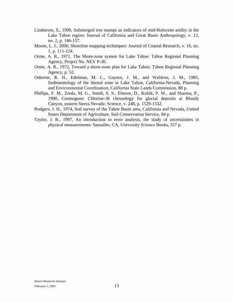
Lindstrom, S., 1990, Submerged tree stumps as indicators of mid-Holocene aridity in the Lake Tahoe region: Journal of California and Great Basin Anthropology, v. 12, no. 2, p. 146-157.

Moore, L. J., 2000, Shoreline mapping techniques: Journal of Coastal Research, v. 16, no. 1, p. 111-124.

Orme, A. R., 1971, The Shore-zone system for Lake Tahoe: Tahoe Regional Planning Agency, Project No. NEV P-30.

Orme, A. R., 1972, Toward a shore-zone plan for Lake Tahoe: Tahoe Regional Planning Agency, p. 52.

Osborne, R. H., Edelman, M. C., Gaynor, J. M., and Waldron, J. M., 1985, Sedimentology of the littoral zone in Lake Tahoe, California-Nevada, Planning and Environmental Coordination, California State Lands Commission, 88 p.

Phillips, F. M., Zreda, M. G., Smith, S. S., Elmore, D., Kubik, P. W., and Sharma, P., 1990, Cosmogenic Chlorine-36 chronology for glacial deposits at Bloody Canyon, eastern Sierra Nevada: Science, v. 248, p. 1529-1532.

Rodgers, J. H., 1974, Soil survey of the Tahoe Basin area, California and Nevada, United States Department of Agriculture, Soil Conservation Service, 84 p.

Taylor, J. R., 1997, An introduction to error analysis, the study of uncertainties in physical measurements: Sausalito, CA, University Science Books, 327 p.

Table 1. Information about aerial photographs used in this study. Year and Photo Scale Agency Location Water Surface Elevation

1938 BPB14-69 1:20,000 USFS Glenbrook Bay 1898.18 m (6227.56 ft) BPB14-75 1:20,000 USFS Zephyr Cove 1898.18 m (6227.56 ft)

1939 CDJ14-51 1:20,000 USFS Sunnyside/Tahoe City 1898.00 m (6226.96 ft) CDJ14-53 1:20,000 USFS Sunnyside/Ward Creek 1898.00 m (6226.96 ft) CDJ14-55 1:20,000 USFS Idlewild/Blackwood Creek 1898.00 m (6226.96 ft) CDJ14-70 1:20,000 USFS Meeks Bay/Rubicon Bay 1898.00 m (6226.96 ft) CDJ14-72 1:20,000 USFS Sugar Pine Point 1898.00 m (6226.96 ft)

CDJ14-72revised 1:20,000 USFS Sugar Pine Point 1898.00 m (6226.96 ft) CDJ14-74 1:20,000 USFS Homewood/Sugar Pine Point 1898.00 m (6226.96 ft) CDJ14-79 1:20,000 USFS Tahoe City 1898.00 m (6226.96 ft) CDJ15-52 1:20,000 USFS Dollar Point 1898.00 m (6226.96 ft) CDJ15-54 1:20,000 USFS Carnelian Bay 1898.00 m (6226.95 ft) CDJ15-56 1:20,000 USFS Carnelian Bay/Agate Bay 1898.00 m (6226.95 ft) CDJ16-44 1:20,000 USFS Agate Bay/Stateline Point 1898.00 m (6226.95 ft) CDJ16-48 1:20,000 USFS Stateline Point/Crystal Bay 1898.00 m (6226.95 ft)

CDJ16-112 1:20,000 USFS Crystal Bay/Incline Village 1898.00 m (6226.95 ft) CDJ17-15 1:20,000 USFS Sand Harbor 1898.00 m (6226.95 ft)

1940 CNL23-2 1:20,000 USFS Rubicon Bay 1898.36 m (6228.15 ft) CNL23-3 1:20,000 USFS Rubicon Point 1898.36 m (6228.15 ft) CNL23-4 1:20,000 USFS Emerald Bay 1898.36 m (6228.15 ft) CNL23-5 1:20,000 USFS Emerald Bay 1898.36 m (6228.15 ft)

CNL23-68 1:20,000 USFS Baldwin Beach 1898.36 m (6228.15 ft) CNL23-74 1:20,000 USFS Camp Richardson/Truckee Marsh 1898.36 m (6228.15 ft)

CNL23-137 1:20,000 USFS Truckee Marsh/South Lake Tahoe 1898.36 m (6228.15 ft) CNL23-140 1:20,000 USFS Nevada Beach/Marla Bay 1898.36 m (6228.15 ft) CNL23-141 1:20,000 USFS Nevada Beach 1898.36 m (6228.15 ft)

1952 ABM3k-63 1:20,000 USFS Carnelian Bay/Agate Bay 1898.52 m (6228.65 ft)

ABM3k-103 1:20,000 USFS Agate Bay/Stateline Point 1898.52 m (6228.65 ft) DSC6k-121 1:20,000 USFS Sugar Pine Point 1898.55 m (6228.75 ft) DSC6k-177 1:20,000 USFS South Lake Tahoe 1898.55 m (6228.75 ft) DSC6k-178 1:20,000 USFS South Lake Tahoe/Nevada Beach 1898.55 m (6228.75 ft)

1992 DOQ 1:12,000 USGS Entire basin 1896.25 m (6221.21 ft)

1995 TAH-12s-47 1:8,000 TRPA Emerald Bay 1897.95 m (6226.80 ft) TAH-12s-49 1:8,000 TRPA Emerald Point 1897.95 m (6226.80 ft) TAH-12s-50 1:8,000 TRPA D.L. Bliss State Park 1897.95 m (6226.80 ft) TAH-13s-2 1:8,000 TRPA Emerald Point/Eagle Point 1897.95 m (6226.80 ft) TAH-13s-4 1:8,000 TRPA Baldwin Beach-west side 1897.95 m (6226.80 ft)

TAH-14s-209 1:8,000 TRPA Baldwin Beach 1897.96 m (6226.84 ft) TAH-15s-154 1:8,000 TRPA Baldwin Beach/Kiva Beach 1897.96 m (6226.84 ft) TAH-16s-153 1:8,000 TRPA Pope Beach 1897.96 m (6226.84 ft) TAH-17s-72 1:8,000 TRPA Pope Beach/Tahoe Keys 1897.96 m (6226.84 ft) TAH-18s-71 1:8,000 TRPA Tahoe Keys/Upper Truckee River 1897.96 m (6226.84 ft)

TAH-19s-207 1:8,000 TRPA Truckee Marsh/South Lake Tahoe 1897.96 m (6226.84 ft) TAH-20s-205 1:8,000 TRPA S. Lake Tahoe 1897.96 m (6226.84 ft) TAH-21s-144 1:8,000 TRPA Nevada Beach 1897.96 m (6226.84 ft) TAH-21s-146 1:8,000 TRPA Stateline/Edgewood Golf Course 1897.96 m (6226.84 ft) TAH-21s-148 1:8,000 TRPA South Lake Tahoe 1897.96 m (6226.84 ft)

1998 DOQ 1:12,000 USGS Entire basin 1898.50 m (6228.61 ft)

Table 2. Nutrient sample data. All location data is referenced to UTM Zone 10.Lab # Sample Name Sample Date Easting Northing TPO4 (mgP/kg) TKN (mgN/kg)47356 SB-1 17-May-00 763682 4347495 212 1847357 SB-2 17-May-00 763681 4347521 316 22947358 SB-3 17-May-00 763637 4347520 192 2247359 SB-4 17-May-00 763610 4347540 264 2547360 SB-5 17-May-00 763580 4347562 656 3147361 SB-6 17-May-00 763575 4347559 224 1847362 SB-7 17-May-00 763598 4347635 452 33847363 SB-8 17-May-00 763619 4347653 444 10847364 SB-9 17-May-00 763544 4347581 172 2247365 SB-10 17-May-00 763499 4347606 740 3747366 SB-11 17-May-00 763474 4347624 756 9747367 SB-12 17-May-00 763449 4347637 1800 1647368 SB-13 17-May-00 763396 4347657 960 3747369 SB-14 17-May-00 763409 4347669 572 17147370 SB-15 17-May-00 763450 4347671 408 21647371 KB-1 17-May-00 757082 4346895 4 3347372 KB-2 17-May-00 757021 4346930 92 7647373 KB-3 17-May-00 756940 4346962 55 3547374 KB-4 17-May-00 756920 4346986 40 6747375 KB-5 17-May-00 756882 4346986 47 3247376 KB-6 17-May-00 756832 4347008 54 3947377 KB-7 17-May-00 756788 4347005 100 1847378 KB-8 17-May-00 756763 4347011 58 1547379 KB-9 17-May-00 756751 4347038 16 6747380 KB-10 17-May-00 756687 4347046 55 3947381 SPP-1 18-May-00 749888 4326641 320 2047382 SPP-2 18-May-00 749927 4326294 168 2047383 SPP-3 18-May-00 749947 4326252 148 27447384 SPP-4 18-May-00 749955 4326256 328 21847385 SPP-5 18-May-00 749955 4326256 272 3247386 SPP-6 18-May-00 749998 4326140 784 92647387 SPP-7 18-May-00 750030 4326073 79 433047388 SPP-8 18-May-00 750026 4326079 584 62848708 SPP-9A 4-Aug-00 749805 4326977 299 29748709 SPP-9B 4-Aug-00 749805 4326977 205 21948710 SPP-9C 4-Aug-00 749805 4326977 172 8348711 SPP-9D 4-Aug-00 749805 4326977 477 5048712 SPP-10A 4-Aug-00 749809 4327071 484 16748713 SPP-10B 4-Aug-00 749809 4327071 445 6248714 SPP-10C 4-Aug-00 749809 4327071 171 20347389 BB-1 18-May-00 745806 4332280 648 5847390 BB-2 18-May-00 745784 4332237 576 4147391 BB-3 18-May-00 745774 4332222 740 5647392 BB-4 18-May-00 745749 4332187 624 5147393 BB-5 18-May-00 745732 4332153 636 6747394 LF-1 17-May-00 749414 4340749 729 132047395 LF-2 17-May-00 749342 4340675 328 6147396 LF-3 17-May-00 749291 4340628 1410 1950

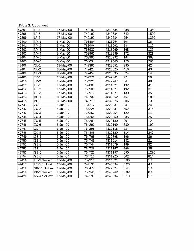
Table 2. Continued47397 LF-4 17-May-00 749197 4340634 388 136047398 LF-5 17-May-00 749197 4340634 542 152047399 LF-6 17-May-00 749197 4340634 254 136047400 NV-1 3-May-00 763884 4318954 80 1847401 NV-2 3-May-00 763904 4318962 88 11247402 NV-3 3-May-00 763930 4318969 168 13647403 NV-4 3-May-00 763962 4318989 172 32147404 NV-5 3-May-00 763995 4318992 164 36347405 NV-6 3-May-00 764034 4319003 128 26547406 CL-1 18-May-00 747392 4328651 380 4247407 CL-2 18-May-00 747427 4328625 416 4347408 CL-3 18-May-00 747454 4328595 324 14547409 TV-1 17-May-00 754976 4347261 72 5047410 TV-2 17-May-00 754925 4347267 64 48647411 UT-1 17-May-00 759883 4314321 132 4147412 UT-2 17-May-00 759900 4314321 192 3147413 UT-3 17-May-00 759910 4314321 130 3547414 BC-1 18-May-00 745737 4332362 467 18547415 BC-2 18-May-00 745719 4332376 506 13947741 ZC-1 6-Jun-00 764212 4322331 84 2447742 ZC-2 6-Jun-00 764224 4322331 552 31547743 ZC-3 6-Jun-00 764250 4322254 122 1147744 ZC-4 6-Jun-00 764268 4322250 285 25847745 ZC-5 6-Jun-00 764281 4322180 90 1247746 ZC-6 6-Jun-00 764293 4322169 330 19947747 ZC-7 6-Jun-00 764298 4322118 62 1147748 ZC-8 6-Jun-00 764308 4322120 114 24047749 GB-1 6-Jun-00 764768 4330898 196 3647750 GB-2 6-Jun-00 764749 4331014 132 2147751 GB-3 6-Jun-00 764744 4331079 189 3247752 GB-4 6-Jun-00 764726 4331157 266 2547753 GB-5 6-Jun-00 764722 4331197 690 127047754 GB-6 6-Jun-00 764713 4331225 502 81447416 UT-3 Soil ext. 17-May-00 759910 4314321 0.06 1.247417 LF-6 Soil ext. 17-May-00 749197 4340634 0.23 4.247418 SB-11 Soil ext. 17-May-00 763474 4347624 0.44 1.647419 KB-3 Soil ext. 17-May-00 756940 4346962 0.02 0.647420 NV-4 Soil ext. 17-May-00 749197 4340634 0.13 1.9

Table 3. Locations of eroded shorezones and sediment and nutrient calculations for those areas.ID Location Material type Area (m^2) Thickness (m)Volume (m^3) Mass (kg) P (mg/kg) N (mg/kg) Tot P (MT) Tot N (MT)

1 Nevada Beach-Stateline old granitic beach sand 21898 1 21898 32847000 280 330 9.20 10.842 Stateline old granitic beach sand 361 1 361 541500 280 330 0.15 0.183 Bijou Park old granitic beach sand 11644 1 11644 17466000 280 330 4.89 5.764 Al Tahoe-Regan Beach old granitic beach sand 11275 6 67650 101475000 280 330 28.41 33.495 Upper Truckee River granitic beach sand 31643 1 31643 47464500 150 35 7.12 1.666 Tahoe Keys old granitic beach sand 1234 1 1234 1851000 280 330 0.52 0.617 Kiva Beach-Camp Richardson old granitic beach sand 10272 2 20544 30816000 280 330 8.63 10.178 Baldwin Beach old granitic beach sand 13600 1 13600 20400000 280 330 5.71 6.739 SE shore of Emerald Bay glacial till 15544 2 31088 46632000 315 120 14.69 5.60

10 Emerald Bay-Vikingsholm glacial till 8304 1 8304 12456000 315 120 3.92 1.4911 Meeks Bay old granitic beach sand 6996 1 6996 10494000 280 330 2.94 3.4612 Sugar Pine Point old granitic beach sand 4008 3 12024 18036000 280 330 5.05 5.9513 Homewood volcanic beach sand 18813 1 18813 28219500 320 230 9.03 6.4914 Tahoe Tavern volcanic beach sand 9545 1 9545 14317500 320 230 4.58 3.2915 Lake Forest gravelly silt 1962 1 1962 2943000 395 1415 1.16 4.1616 Carnelian Bay volcanic beach sand 8160 1 8160 12240000 320 230 3.92 2.8217 Agate Bay volcanic beach sand 4562 2 9124 13686000 320 230 4.38 3.1518 Tahoe Vista volcanic beach sand 3449 1 3449 5173500 68 270 0.35 1.4019 Brockway old granitic beach sand 1190 1 1190 1785000 280 330 0.50 0.5920 Kings Beach-west side volcanic beach sand 728 1 728 1092000 50 40 0.05 0.0421 Kings Beach-east side volcanic beach sand 903 2 1806 2709000 50 40 0.14 0.1122 Glenbrook old granitic beach sand 4471 1 4471 6706500 280 330 1.88 2.21

P NTOTALS = 190562 286234 429,351,000 TOTALS (MT)= 117 110

Table 4. Yearly sources for nitrogen and phosphorous for Lake Tahoe in metric tons.

Source comparison: *Working Draft of Lake Tahoe Watershed Assessment. #Estimates from the Watershed Assessment for yearly contributions of nitrogen and phosphorous

were 0.75 and 0.45 metric tons, respectively. **From this study.

Nutrient Inputs Total N (MT) Total P (MT) Atmospheric deposition* 233.9 (56%) 12.4 (26%) Stream loading* 81.6 (20%) 13.3 (28%) Direct runoff* 41.8 (10%) 15.5 (33%) Groundwater* 60 (14%) 4 (9%) Shorezone erosion#,** 1.8 (<1%) 2 (4%)

0.63

4.74.565.84

5.19

4.90

1.46

1.17

3.84

5.46

9.96

10. 62

4.3

0 10 20 km

N

ExplanationWaterbodiesGraniticsVolcanicsGlacial morainesAlluvial and lacustrine sediments

Figure 1. Simplified geologic map of the Lake Tahoe basin showing the distribution of rocks and sediment.

Lake Tahoe levels from 1900 to 2000

6219

6220

6221

6222

6223

6224

6225

6226

6227

6228

6229

6230

6231

6232

1900 1905 1910 1915 1920 1925 1930 1935 1940 1945 1950 1955 1960 1965 1970 1975 1980 1985 1990 1995 2000

Year

Ele

vati

on

(fe

et)

Figure 2. Lake level fluctuations in Lake Tahoe from 1900 to 2000.

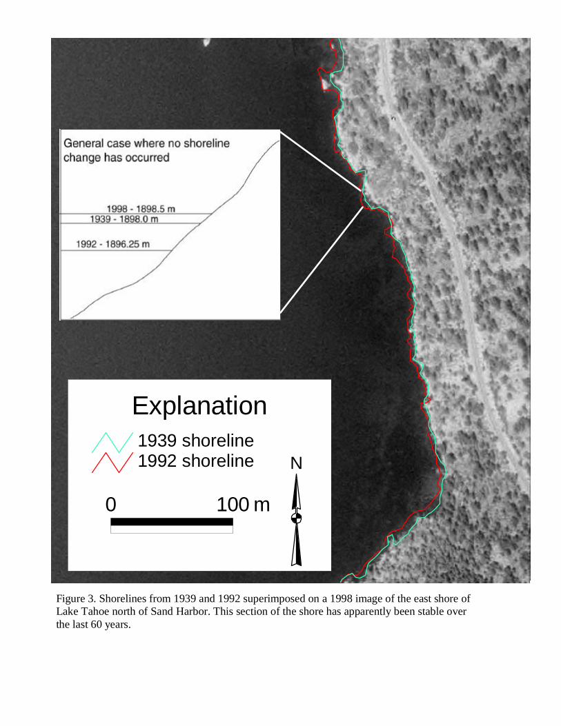
1992 shoreline1939 shoreline

Explanation

0 100 m

N

Figure 3. Shorelines from 1939 and 1992 superimposed on a 1998 image of the east shore of Lake Tahoe north of Sand Harbor. This section of the shore has apparently been stable overthe last 60 years.

Areas of erosion1992 shoreline1939 shoreline

Explanation

N

Figure 4. Shorelines from 1939 and 1992 superimposed on a 1998 image of the Homewood area. In this case, erosion is indicated because the 1939 shoreline (1898.0 m) is coincident with the 1992 shoreline (1896.25 m) along part of its length.

0 100 m

#

##

#

#

##

BB-1

BB-2

BB-3BB-4

BB-5

BC-1BC-2

Areas of accretion1939 shoreline

# Nutrient samples

Explanation

N

Figure 5. The shoreline from 1939 superimposed on an image of Blackwood Creek from 1998. Note that the shore has built lakeward even though lake level in 1939 was about one half meter below that in 1998.

0 100 m

Areas of accretionAreas of erosion1952 shoreline1940 shoreline

Explanation

Figure 6. Shorelines from 1940 and 1952 superimposed on a 1998 image from Edgewood Golf Course along the southeast shore of Lake Tahoe. In this case, there was accretion from 1940 to 1952 and then erosion from 1952 to the present.

0 100 m

N

10.6o

10.6o

10.6o

0.5 m

1998 193912 m

67 .26.10tan

5.0= m

1998

1992

2.25 m

Figure 7a

Figure 7b

12 m

q

arctan 2.2512

= q =10.6

Figure 7. Schematic diagram showing how the amount of shoreline erosion is calculatedfrom air photos that reflect different lake levels. Figure 7a shows how the overall slope is calculated from the 1992 and 1998 DOQ's. Figure 7b shows how this slope is used to estimate where the 1939 shoreline would project if lake level was the same as when the 1998 image was taken. In this case, about 9 m of apparent erosion has occurred because,given a slope of 10.6 degrees, the projected 1939 lake level would only move up the beachabout 2.67 m but the 1998 shoreline is 12 m away. The approximately 9 m of difference between these figures represents erosion.

###############

##########

########

#####

######

######

###

##

###

##

########

######

######

#Historic stump ~ 4 m from shor e

SB-1SB-2SB-3SB-4

SB-5SB-6

SB-7SB-8

SB-9

KB-1

KB-2KB-3

KB-4KB-5KB-6KB-7KB-8KB-9

BB-1

BB-2

BB-3BB-4

BB-5

LF -1

LF -2

LF -3LF -4LF -5LF -6

NV- 1NV- 2NV- 3NV- 4NV- 5NV- 6

CL-1CL-2

CL-3

TV-1TV-2

UT-1UT-2UT-3

BC- 1BC- 2

ZC-1ZC-2

ZC-3ZC-4

ZC-5ZC-6

ZC-7ZC-8

GB- 1

GB- 2

GB- 3

GB- 4

GB- 5GB- 6

SB-10SB-11SB-12SB-13SB-14SB-15

KB-10

SPP- 1

SPP- 2

SPP- 3SPP- 4SPP- 5

SPP- 6

SPP- 7SPP- 8

SPP- 9ASPP- 9BSPP- 9C

SPP- 10ASPP- 10BSPP- 10C

SPP- 9D

TahoeoutlineAccretionErosion

# Nutrient samples

0 10 km

N

Figure 8. Map showing areas at Lake Tahoe that have undergone erosion or accretion since 1939. Also shown are nutrient sample locations.