himanshu tyagi - university of california, san diegocommon randomness principles of secrecy himanshu...
TRANSCRIPT

Common Randomness Principles of Secrecy
Himanshu Tyagi
Department of Electrical and Computer Engineering
and Institute of Systems Research

Correlated Data, Distributed in Space and Time
SecurityHardwareSensor
NetworksBiometricSecurity
CloudComputing
1

Secure Processing of Distributed Data
Three classes of problems are studied:
1. Secure Function Computation with Trusted Parties
2. Communication Requirements for Secret Key Generation
3. Querying Eavesdropper
2

Secure Processing of Distributed Data
Three classes of problems are studied:
1. Secure Function Computation with Trusted Parties
2. Communication Requirements for Secret Key Generation
3. Querying Eavesdropper
Our Approach
◮ Identify the underlying common randomness
◮ Decompose common randomness into independent components
2

Outline
1. Basic Concepts
2. Secure Computation
3. Minimal Communication for Optimum Rate Secret Keys
4. Querying Common Randomness
5. Principles of Secrecy Generation
3

Basic Concepts
Multiterminal Source Model
Interactive Communication Protocol
Common Randomness
Secret Key
4

Multiterminal Source Model
XnmXn
1 Xn2
Assumption on the data
◮ Xni = (Xi1, ...,Xin)
- Data observed at time instance t: XMt = (X1t, ...,Xmt)
- Probability distribution of X1, ...,Xm is known.
◮ Observations are i.i.d. across time:
- XM1, ...,XMn are i.i.d. rvs.
◮ Observations are finite-valued.
5

Interactive Communication Protocol
COMMUNICATION NETWORK
F11
Xn1 Xn
2 Xnm
Assumptions on the protocol
◮ Each terminal has access to all the communication.
◮ Multiple rounds of interactive communication are allowed.
◮ Communication from terminal 1: F11 = f11 (Xn1 )
6
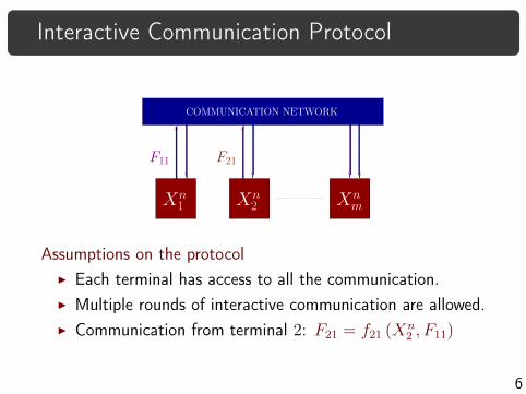
Interactive Communication Protocol
COMMUNICATION NETWORK
F11 F21
Xn1 Xn
2 Xnm
Assumptions on the protocol
◮ Each terminal has access to all the communication.
◮ Multiple rounds of interactive communication are allowed.
◮ Communication from terminal 2: F21 = f21 (Xn2 , F11)
6

Interactive Communication Protocol
COMMUNICATION NETWORK
F1 F2 Fm
Xn1 Xn
2 Xnm
Assumptions on the protocol
◮ Each terminal has access to all the communication.
◮ Multiple rounds of interactive communication are allowed.
◮ r rounds of interactive communication: F = F1, ...,Fm
6

Common Randomness
COMMUNICATION NETWORK
A
L1 L2
F
Xn1 Xn
2 Xnm
Definition. L is an ǫ-common randomness for A from F if
P (L = Li(Xni ,F), i ∈ A) ≥ 1− ǫ
Ahlswede-Csiszár ’93 and ’98. 7

Secret Key
COMMUNICATION NETWORK
A F
Xn1 Xn
2 Xnm
K K
Definition. An rv K ∈ K is an ǫ-secret key for A from F if
1. Recoverability: K is an ǫ-CR for A from F
2. Security: K is concealed from an observer of F
Maurer ’93 Ahlswede-Csiszár ’93 Csiszár-Narayan ’04. 8

Secret Key
COMMUNICATION NETWORK
A F
Xn1 Xn
2 Xnm
K K
Definition. An rv K ∈ K is an ǫ-secret key for A from F if
1. Recoverability: K is an ǫ-CR for A from F
2. Security: K is concealed from an observer of F
PKF ≈ UK × PF
Maurer ’93 Ahlswede-Csiszár ’93 Csiszár-Narayan ’04. 8

Notions of Security
◮ Kullback-Leibler Divergence
sin(K,F) = D (PKF‖UK × PF)
= log |K| −H(K) + I(K ∧ F) ≈ 0
◮ Variational Distance
svar(K,F) = ‖PKF − UK × PF‖1 ≈ 0
◮ Weak
sweak(K,F) =1
nsin(K,F) ≈ 0
9

Notions of Security
◮ Kullback-Leibler Divergence
sin(K,F) = D (PKF‖UK × PF)
= log |K| −H(K) + I(K ∧ F) ≈ 0
◮ Variational Distance
svar(K,F) = ‖PKF − UK × PF‖1 ≈ 0
◮ Weak
sweak(K,F) =1
nsin(K,F) ≈ 0
2 svar(K,F)2 ≤ sin(K,F) ≤ svar(K,F) log |K|svar(K,F)
9

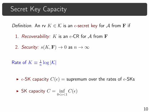
Secret Key Capacity
Definition. An rv K ∈ K is an ǫ-secret key for A from F if
1. Recoverability: K is an ǫ-CR for A from F
2. Security: s(K,F) → 0 as n → ∞
10

Secret Key Capacity
Definition. An rv K ∈ K is an ǫ-secret key for A from F if
1. Recoverability: K is an ǫ-CR for A from F
2. Security: s(K,F) → 0 as n → ∞
Rate of K ≡ 1nlog |K|
10
Secret Key Capacity
Definition. An rv K ∈ K is an ǫ-secret key for A from F if
1. Recoverability: K is an ǫ-CR for A from F
2. Security: s(K,F) → 0 as n → ∞
Rate of K ≡ 1nlog |K|
◮ ǫ-SK capacity C(ǫ) = supremum over the rates of ǫ-SKs
◮ SK capacity C = inf0<ǫ<1
C(ǫ)
10

Secret Key Capacity
Theorem (Csiszár-Narayan ’04)
The SK capacity is given by
C = H (XM)− RCO,
where
RCO = minm∑
i=1
Ri,
such that∑
i∈B Ri ≥ H (XB | XBc), for all A * B ⊆ M.
11

Secret Key Capacity
RCO ≡ min. rate of “communication for omniscience" for A
Theorem (Csiszár-Narayan ’04)
The SK capacity is given by
C = H (XM)− RCO,
where
RCO = minm∑
i=1
Ri,
such that∑
i∈B Ri ≥ H (XB | XBc), for all A * B ⊆ M.
11

Secret Key Capacity
RCO ≡ min. rate of “communication for omniscience" for A
Theorem (Csiszár-Narayan ’04)
The SK capacity is given by
C = H (XM)− RCO,
where
RCO = minm∑
i=1
Ri,
such that∑
i∈B Ri ≥ H (XB | XBc), for all A * B ⊆ M.
(Maurer ’93, Ahlswede-Csiszár ’93)
For m = 2: C = I(X1 ∧X2)
11

Secure Computation
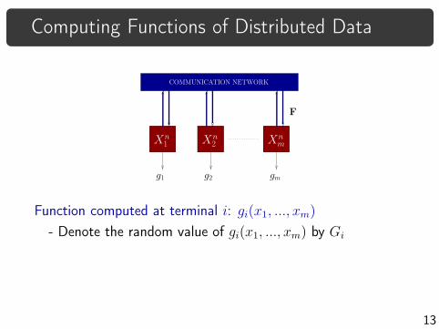
Computing Functions of Distributed Data
COMMUNICATION NETWORK
F
Xn1 Xn
2 Xnm
g2g1 gm
Function computed at terminal i: gi(x1, ..., xm)
- Denote the random value of gi(x1, ..., xm) by Gi
13

Computing Functions of Distributed Data
COMMUNICATION NETWORK
F
Xn1 Xn
2 Xnm
g2g1 gm
Function computed at terminal i: gi(x1, ..., xm)
- Denote the random value of gi(x1, ..., xm) by Gi
P(
Gni = G
(n)i (Xn
i ,F), for all 1 ≤ i ≤ m)
≥ 1− ǫ
13

Secure Function Computation
COMMUNICATION NETWORK
F
Xn1 Xn
2 Xnm
g2g1 gm
I(Gn0 ∧ F) ≈ 0
Value of private function g0 must not be revealed
Definition. Functions g0, g1, ..., gm are securely computable if
1. Recoverability: P(
Gni = G
(n)i (Xn
i ,F), i ∈ M)
→ 1
2. Security: I(Gn0 ∧ F) → 0
14

Secure Function Computation
When are functions g0, g1, ..., gm securely computable?
COMMUNICATION NETWORK
F
Xn1 Xn
2 Xnm
g2g1 gm
I(Gn0 ∧ F) ≈ 0
Value of private function g0 must not be revealed
Definition. Functions g0, g1, ..., gm are securely computable if
1. Recoverability: P(
Gni = G
(n)i (Xn
i ,F), i ∈ M)
→ 1
2. Security: I(Gn0 ∧ F) → 0
14

Secure Function Computation
When is a function g securely computable?
COMMUNICATION NETWORK
F
Xn1 Xn
2 Xnm
g g g
I(Gn ∧ F) ≈ 0
Value of Private function g0 = g
Definition. Function g is securely computable if
1. Recoverability: P(
Gn = G(n)i (Xn
i ,F), i ∈ M)
→ 1
2. Security: I(Gn ∧ F) → 0
15

A Necessary Condition
If g is securely computable, then it constitutes an SK for M.
Therefore,rate of G ≤ SK Capacity,
i.e.,
H(G) ≤ C.
16
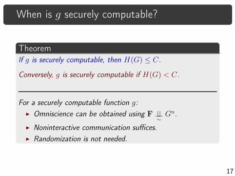
When is g securely computable?
TheoremIf g is securely computable, then H(G) ≤ C.
Conversely, g is securely computable if H(G) < C.
For a securely computable function g:
◮ Omniscience can be obtained using F ⊥⊥∼
Gn.
◮ Noninteractive communication suffices.
◮ Randomization is not needed.
17

Example: Secure Computation using Secret Keys
H(K) = 1
B1 B2K K
Secret Key K
g(X1, X2) = B1 ⊕ B2
X1 X2
18

Example: Secure Computation using Secret Keys
H(K) = 1
B1 B2K K
Secret Key K
g(X1, X2) = B1 ⊕ B2
X1 X2
B1
18

Example: Secure Computation using Secret Keys
H(K) = 1
B1 B2K K
Secret Key K
g(X1, X2) = B1 ⊕ B2
X1 X2
K ⊕ B1 ⊕ B2
B1
18
Example: Secure Computation using Secret Keys
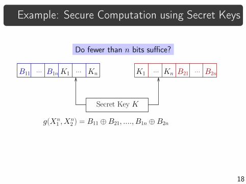
Do fewer than n bits suffice?
B2n
Secret Key K
g(Xn1 , X
n2 ) = B11 ⊕ B21, ...., B1n ⊕ B2n
K1 Kn...B1n
...B11... KnK1 B21
...
18

Example: Secure Computation using Secret Keys
Do fewer than n bits suffice?
B2n
Secret Key K
g(Xn1 , X
n2 ) = B11 ⊕ B21, ...., B1n ⊕ B2n
K1 Kn...B1n
...B11... KnK1 B21
...
◮ If parity is securely computable:
1 = H(G) ≤ C = H(K)
18
Characterization of Secure Computability
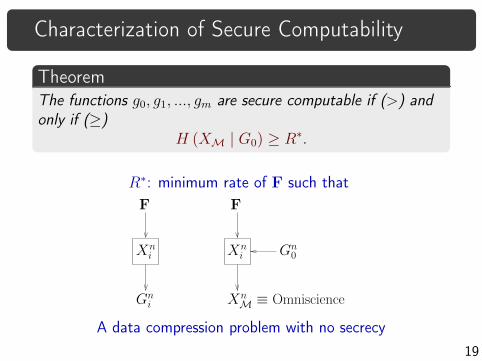
TheoremThe functions g0, g1, ..., gm are secure computable if (>) andonly if (≥)
H (XM | G0) ≥ R∗.
R∗: minimum rate of F such that
Xni
Gni
Gn0
F
XnM ≡ Omniscience
F
Xni
A data compression problem with no secrecy
19

Example: Functions of Binary Sources
h(δ)
1
δ
δ
1− δ
1− δX2
0
Pr(X1 6= X2) = δ
δ
1
δ = 0.5
X1
0
1
Pr(X1 = 1) = 12
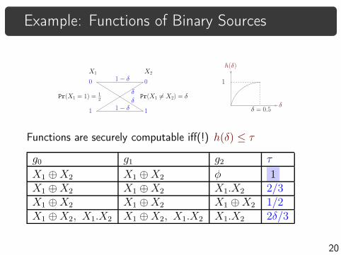
Functions are securely computable iff(!) h(δ) ≤ τ
g0 g1 g2 τX1 ⊕X2 X1 ⊕X2 φ 1X1 ⊕X2 X1 ⊕X2 X1.X2 2/3X1 ⊕X2 X1 ⊕X2 X1 ⊕X2 1/2X1 ⊕X2, X1.X2 X1 ⊕X2, X1.X2 X1.X2 2δ/3
20
Example: Functions of Binary Sources
h(δ)
1
δ
δ
1− δ
1− δX2
0
Pr(X1 6= X2) = δ
δ
1
δ = 0.5
X1
0
1
Pr(X1 = 1) = 12
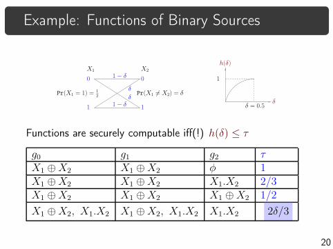
Functions are securely computable iff(!) h(δ) ≤ τ
g0 g1 g2 τ
X1 ⊕X2 X1 ⊕X2 φ 1X1 ⊕X2 X1 ⊕X2 X1.X2 2/3X1 ⊕X2 X1 ⊕X2 X1 ⊕X2 1/2X1 ⊕X2, X1.X2 X1 ⊕X2, X1.X2 X1.X2 2δ/3
20
Example: Functions of Binary Sources
h(δ)
1
δ
δ
1− δ
1− δX2
0
Pr(X1 6= X2) = δ
δ
1
δ = 0.5
X1
0
1
Pr(X1 = 1) = 12
Functions are securely computable iff(!) h(δ) ≤ τ
g0 g1 g2 τX1 ⊕X2 X1 ⊕X2 φ 1X1 ⊕X2 X1 ⊕X2 X1.X2 2/3X1 ⊕X2 X1 ⊕X2 X1 ⊕X2 1/2
X1 ⊕X2, X1.X2 X1 ⊕X2, X1.X2 X1.X2 2δ/3
20
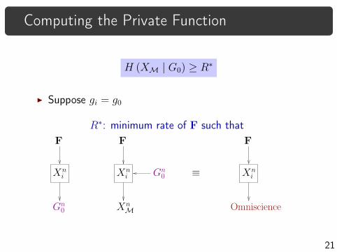
Computing the Private Function
H (XM | G0) ≥ R∗
◮ Suppose gi = g0
R∗: minimum rate of F such that
≡
F
Omniscience
XniGn
0
F
XnM
F
Gn0
Xni Xn
i
21

Computing the Private Function
H (XM | G0) ≥ R∗
◮ Suppose gi = g0
R∗: minimum rate of F such that
≡
F
Omniscience
XniGn
0
F
XnM
F
Gn0
Xni Xn
i
21
If g0 is securely computable at a terminal thenthe entire data can be recovered securely at that terminal

Minimal Communication for an
Optimum Rate Secret Key

Secret Key Generation for Two Terminals
COMMUNICATION NETWORK
F
Xn2
K
Xn1
K
Weak secrecy criterion: 1nsin(K,F) → 0.
Secret key capacity C = I(X1 ∧X2)
Maurer ’93 Ahlswede-Csiszár ’93
23

Common Randomness for SK Capacity
What is the form of CR that yields an optimum rate SK?
◮ Maurer-Ahlswede-Csiszár
Common randomness generated
Xn1 or Xn
2
Rate of communication required
min{H(X1|X2),H(X2|X1)}
Decomposition
H(X1) = H(X1|X2) + I(X1 ∧X2)
H(X2) = H(X2|X1) + I(X1 ∧X2)
24

Digression: Secret Keys and Biometric Security
Public Server
X1
Secure Server
F (X1)
K(X1)
25
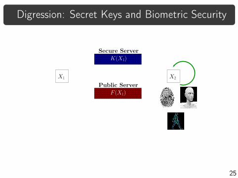
Digression: Secret Keys and Biometric Security
F (X1)
X1
Secure Server
K(X1)
Public Server
X2
25

Digression: Secret Keys and Biometric Security
Public Server
Secure Server
K(X1)
F (X1)
=?
X2
25
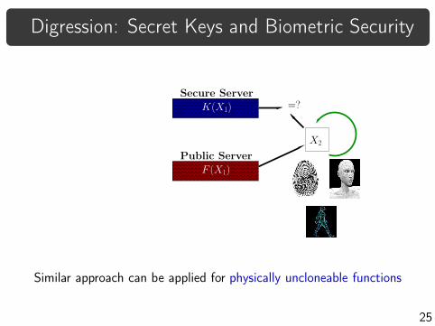
Digression: Secret Keys and Biometric Security
Public Server
Secure Server
K(X1)
F (X1)
=?
X2
Similar approach can be applied for physically uncloneable functions
25

Common Randomness for SK Capacity
What is the form of CR that yields an optimum rate SK?
◮ Maurer-Ahlswede-Csiszár
Common randomness generated
Xn
1or Xn
2
Rate of communication required
min{H(X1|X2), H(X2|X1)}
Decomposition
H(X1) = H(X1|X2) + I(X1 ∧X2)H(X2) = H(X2|X1) + I(X1 ∧X2)
26

Common Randomness for SK Capacity
What is the form of CR that yields an optimum rate SK?
◮ Maurer-Ahlswede-Csiszár Csiszár-Narayan
Common randomness generated
Xn
1or Xn
2(Xn
1, Xn
2)
Rate of communication required
min{H(X1|X2), H(X2|X1)} H(X1|X2) +H(X2|X1)
Decomposition
H(X1) = H(X1|X2) + I(X1 ∧X2)H(X2) = H(X2|X1) + I(X1 ∧X2)
H(X1, X2) = H(X1|X2) +H(X2|X1) + I(X1 ∧X2)
26

Characterization of CR for Optimum Rate SK
TheoremA CR J recoverable from F yields an optimum rate SK iff
1
nI (Xn
1 ∧Xn2 |J,F) → 0.
Examples: Xn1 or Xn
2 or (Xn1 , X
n2 )
27

Interactive Common Information
◮ Interactive Common Information
Let J be a CR from communication F.
CIri (X1;X2) ≡ min. rate of L = (J,F) such that
1
nI(Xn
1 ∧Xn2 |L) → 0 (∗)
CIi(X1 ∧X2) := limr→∞
CIri (X1;X2)
28

Interactive Common Information
◮ Interactive Common Information
Let J be a CR from communication F.
CIri (X1;X2) ≡ min. rate of L = (J,F) such that
1
nI(Xn
1 ∧Xn2 |L) → 0 (∗)
CIi(X1 ∧X2) := limr→∞
CIri (X1;X2)
◮ Wyner’s Common Information
CI(X1 ∧X2) ≡ min. rate of L (Xn1 ,X
n2 ) s.t. (∗) holds
28

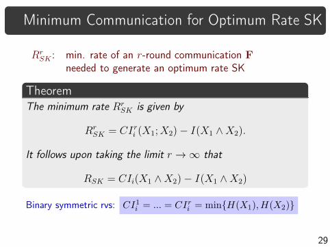
Minimum Communication for Optimum Rate SK
RrSK : min. rate of an r-round communication F
needed to generate an optimum rate SK
TheoremThe minimum rate Rr
SK is given by
RrSK = CIri (X1;X2)− I(X1 ∧X2).
It follows upon taking the limit r → ∞ that
RSK = CIi(X1 ∧X2)− I(X1 ∧X2)
A single letter characterization of CIri is available.
29
Minimum Communication for Optimum Rate SK
RrSK : min. rate of an r-round communication F
needed to generate an optimum rate SK
TheoremThe minimum rate Rr
SK is given by
RrSK = CIri (X1;X2)− I(X1 ∧X2).
It follows upon taking the limit r → ∞ that
RSK = CIi(X1 ∧X2)− I(X1 ∧X2)
Binary symmetric rvs: CI1i = ... = CIri = min{H(X1),H(X2)}
29

Minimum Communication for Optimum Rate SK
RrSK : min. rate of an r-round communication F
needed to generate an optimum rate SK
TheoremThe minimum rate Rr
SK is given by
RrSK = CIri (X1;X2)− I(X1 ∧X2).
It follows upon taking the limit r → ∞ that
RSK = CIi(X1 ∧X2)− I(X1 ∧X2)
There is an example with CI1i > CI2i ⇒ Interaction does help!
29

Common Information Quantities
CIGC ≤ I(X1 ∧X2) ≤ CI ≤ CIi ≤ min{H(X1),H(X2)}
30

Common Information Quantities
CIGC ≤ I(X1 ∧X2) ≤ CI ≤ CIi ≤ min{H(X1),H(X2)}
30

Common Information Quantities
CIGC ≤ I(X1 ∧X2) ≤ CI ≤ CIi ≤ min{H(X1),H(X2)}
30

Common Information Quantities
CIGC ≤ I(X1 ∧X2) ≤ CI ≤ CIi ≤ min{H(X1),H(X2)}
30

Common Information Quantities
CIGC ≤ I(X1 ∧X2) ≤ CI ≤ CIi ≤ min{H(X1),H(X2)}
Interactive Common Information
30

Common Information Quantities
CIGC ≤ I(X1 ∧X2) ≤ CI ≤ CIi ≤ min{H(X1),H(X2)}
Interactive Common Information
◮ CIi is indeed a new quantity
Binary symmetric rvs: CI < min{H(X1),H(X2)} = CIi.
30

Querying Common Randomness

Common Randomness
COMMUNICATION NETWORK
A
L1 L2
F
Xn1 Xn
2 Xnm
Definition. L is an ǫ-common randomness for A from F if
P (L = Li(Xni ,F), i ∈ A) ≥ 1− ǫ
Ahlswede-Csiszár ’93 and ’98. 32

Query Strategy
q(ut | v) = t
V = v no
u1 ut
no
q(u1 | v) = 1
yes yes
Is U = u1? Is U = ut?
Query strategy for U given V
Massey ’94, Arikan ’96, Arikan-Merhav ’99, Hanawal-Sundaresan ’11
33

Query Strategy
Given rvs U, V with values in the sets U ,V.
Definition. A query strategy q for U given V = v is a bijection
q(·|v) : U → {1, ..., |U|},
where the querier, upon observing V = v, asks the question
“Is U = u?"
in the q(u|v)th query.
q(U |V ): random query number for U upon observing V
34

Query Strategy
Given rvs U, V with values in the sets U ,V.
Definition. A query strategy q for U given V = v is a bijection
q(·|v) : U → {1, ..., |U|},
where the querier, upon observing V = v, asks the question
“Is U = u?"
in the q(u|v)th query.
q(U |V ): random query number for U upon observing V
|{u : q(u | v) < γ}| < γ
34

Optimum Query Exponent
Definition. E ≥ 0 is an ǫ-achievable query exponent if
there exists ǫ-CR Ln for A from Fn such that
supq
P(
q(Ln | Fn) < 2nE)
→ 0 as n → ∞,
where the sup is over every query strategy for Ln given Fn.
35

Optimum Query Exponent
Definition. E ≥ 0 is an ǫ-achievable query exponent if
there exists ǫ-CR Ln for A from Fn such that
supq
P(
q(Ln | Fn) < 2nE)
→ 0 as n → ∞,
where the sup is over every query strategy for Ln given Fn.
E∗(ǫ) , sup{E : E is an ǫ-achievable query exponent}
E∗ , inf0<ǫ<1
E∗(ǫ) : optimum query exponent
35
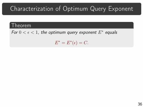
Characterization of Optimum Query Exponent
TheoremFor 0 < ǫ < 1, the optimum query exponent E∗ equals
E∗ = E∗(ǫ) = C.
36

Characterization of Optimum Query Exponent
TheoremFor 0 < ǫ < 1, the optimum query exponent E∗ equals
E∗ = E∗(ǫ) = C.
Proof.
Achievability: E∗(ǫ) ≥ C(ǫ) - Easy
Converse: E∗(ǫ) ≤ C - Main contribution
36
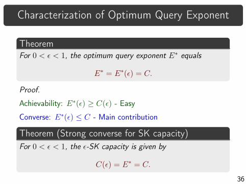
Characterization of Optimum Query Exponent
TheoremFor 0 < ǫ < 1, the optimum query exponent E∗ equals
E∗ = E∗(ǫ) = C.
Proof.
Achievability: E∗(ǫ) ≥ C(ǫ) - Easy
Converse: E∗(ǫ) ≤ C - Main contribution
Theorem (Strong converse for SK capacity)
For 0 < ǫ < 1, the ǫ-SK capacity is given by
C(ǫ) = E∗ = C.
36
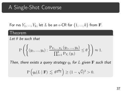
A Single-Shot Converse
For rvs Y1, ..., Yk, let L be an ǫ-CR for {1, ..., k} from F.
TheoremLet θ be such that
P
({
(y1, ..., yk) :PY1,...,Yk
(y1, ..., yk)∏k
i=1 PYi(yi)
≤ θ
})
≈ 1.
Then, there exists a query strategy q0 for L given F such that
P(
q0(L | F) . θ1
k−1
)
≥ (1−√ǫ)2 > 0.
37

Small Cardinality Sets with Large Probabilities
Rényi entropy of order α of a probability measure µ on U :
Hα(µ) ,1
1− αlog∑
u∈U
µ(u)α, 0 ≤ α 6= 1
Lemma. There exists a set Uδ ⊆ U with µ (Uδ) ≥ 1− δ s.t.
|Uδ| . exp (Hα(µ)) , 0 ≤ α < 1.
38

Small Cardinality Sets with Large Probabilities
Rényi entropy of order α of a probability measure µ on U :
Hα(µ) ,1
1− αlog∑
u∈U
µ(u)α, 0 ≤ α 6= 1
Lemma. There exists a set Uδ ⊆ U with µ (Uδ) ≥ 1− δ s.t.
|Uδ| . exp (Hα(µ)) , 0 ≤ α < 1.
Conversely, for any set Uδ ⊆ U with µ (Uδ) ≥ 1− δ,
|Uδ| & exp (Hα(µ)) , α > 1.
1
H(X)
Hα(P )
α
log |X |
38

In Closing ...
Our Approach
◮ Identify the underlying common randomness
◮ Decompose common randomness into independent components
40

Our Approach
◮ Identify the underlying common randomness
◮ Decompose common randomness into independent components
Secure Computing
Common Randomness
Omniscience with side information g0 for decoding
Decomposition
The private function, the communication and the residual randomness
40

Our Approach
◮ Identify the underlying common randomness
◮ Decompose common randomness into independent components
Two Terminal Secret Key Generation
Common Randomness
Renders the observations conditionally independent
Decomposition
The secret key and the communication
40

Our Approach
◮ Identify the underlying common randomness
◮ Decompose common randomness into independent components
Querying Eavesdropper
Requiring the number of queries to be as large as possible
– is tantamount to decomposition into independent parts
40

Prin iples of Se re y GenerationComputing the private function g0 at a terminal is as difficultas securely recovering the entire data at that terminal.
A CR yields an optimum rate SK iff it renders the observationsof the two terminals (almost) conditionally independent.
Almost independence secrecy criterion is equivalent to imposinga lower bound on the complexity of a querier of the secret.
41

Supplementary Slides

Sufficiency
◮ Share all data to compute g: Omniscience ≡ XnM
◮ Can we attain omniscience using F ⊥⊥∼
Gn?
Total randomness: H(XM)
the randomness: RCO
Entropy of G
Communication required to share
Claim: Omniscience can be attained using F ⊥⊥∼
Gn if:
H(G) < H (XM)− RCO
.43
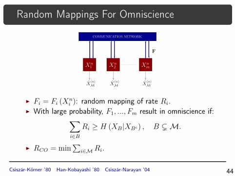
Random Mappings For Omniscience
COMMUNICATION NETWORK
F
Xn1 Xn
2 Xnm
X(n)M X
(n)MX
(n)M
◮ Fi = Fi (Xni ): random mapping of rate Ri.
◮ With large probability, F1, ..., Fm result in omniscience if:∑
i∈B
Ri ≥ H (XB|XBc) , B ( M.
◮ RCO = min∑
i∈M Ri.
Csiszár-Körner ’80 Han-Kobayashi ’80 Csiszár-Narayan ’04 44
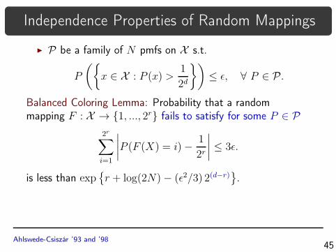
Independence Properties of Random Mappings
◮ P be a family of N pmfs on X s.t.
P
({
x ∈ X : P (x) >1
2d
})
≤ ǫ, ∀ P ∈ P.
Balanced Coloring Lemma: Probability that a randommapping F : X → {1, ..., 2r} fails to satisfy for some P ∈ P
2r∑
i=1
∣
∣
∣
∣
P (F (X) = i)− 1
2r
∣
∣
∣
∣
≤ 3ǫ.
is less than exp{
r + log(2N)− (ǫ2/3) 2(d−r)}
.
Ahlswede-Csiszár ’93 and ’9845

Independence Properties of Random Mappings
◮ P be a family of N pmfs on X s.t.
P
({
x ∈ X : P (x) >1
2d
})
≤ ǫ, ∀ P ∈ P.
Balanced Coloring Lemma: Probability that a randommapping F : X → {1, ..., 2r} fails to satisfy for some P ∈ P
2r∑
i=1
∣
∣
∣
∣
P (F (X) = i)− 1
2r
∣
∣
∣
∣
≤ 3ǫ.
is less than exp{
r + log(2N)− (ǫ2/3) 2(d−r)}
.
Generalized Privacy Amplification
Ahlswede-Csiszár ’93 and ’98 Bennett-Brassard-Crépeau-Maurer ’9545

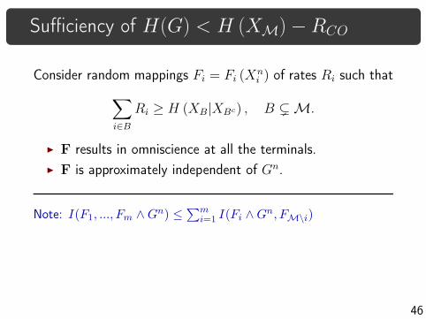
Sufficiency of H(G) < H (XM)−RCO
Consider random mappings Fi = Fi (Xni ) of rates Ri such that
∑
i∈B
Ri ≥ H (XB|XBc) , B ( M.
◮ F results in omniscience at all the terminals.
◮ F is approximately independent of Gn.
46
Sufficiency of H(G) < H (XM)−RCO
Consider random mappings Fi = Fi (Xni ) of rates Ri such that
∑
i∈B
Ri ≥ H (XB|XBc) , B ( M.
◮ F results in omniscience at all the terminals.
◮ F is approximately independent of Gn.
Note: I(F1, ..., Fm ∧Gn) ≤∑mi=1 I(Fi ∧Gn, FM\i)
46

Sufficiency of H(G) < H (XM)−RCO
Consider random mappings Fi = Fi (Xni ) of rates Ri such that
∑
i∈B
Ri ≥ H (XB|XBc) , B ( M.
◮ F results in omniscience at all the terminals.
◮ F is approximately independent of Gn.
Note: I(F1, ..., Fm ∧Gn) ≤∑mi=1 I(Fi ∧Gn, FM\i)
Show I(Fi ∧Gn, FM\i) ≈ 0 with probability close to 1
- using an extension of the BC Lemma [Lemma 2.7]
46