Discussion Papers No. 215, March 1998Statistics Norway, Research Department

Hilde C. Bjørnland

Economic Fluctuations in a SmallOpen Economy – Real versusNominal Shocks

Abstract:This paper analyses the role of real and nominal shocks in explaining business cycles in a small openeconomy like that of Norway. In particular, we study the sources behind real exchange rate fluctuationssince the collapse of the Bretton Woods agreement. Imposing long run restrictions implied by economictheory on a structural vector autoregression (VAR) model containing GDP, unemployment (or price),real wage and the real exchange rate, four structural shocks are identified; Velocity (or monetary),fiscal, productivity and labour supply shocks. The model is also augmented to allow for oil priceshocks.The identified shocks and their impulse responses are consistent with an open economy(Keynesian) model of economic fluctuations, and highlights the exchange rate as a transmissionmechanism in a small open and energy based economy. Especially, I have found a plausible sequenceof shocks (productivity shocks in the 1970s, velocity shocks in the mid-1980s, productivity and laboursupply shocks in the late 1980s, and velocity and fiscal shocks in the early 1990s), which help to explainthe evolution of GDP, unemployment, price, real wage and the real exchange rate. The results arerobust to alternative specifications of the model and are stable over the sample.

Keywords: Real and nominal shocks, exchange rate fluctuations, purchasing power parity, dynamicrestrictions, structural VAR

JEL classification: C32, E32, E63, F41

Acknowledgement: The author wishes to thank Å. Cappelen, C. Kearney, K. Moum, R. Nymoen,A. Rødseth and participants at the Third International Conference on Financial Econometrics inAlaska for very useful comments and discussions. This research was supported by the ResearchCouncil of Norway. The usual disclaimers apply.

Address: Hilde Christiane Bjørnland, Statistics Norway, Research Department. E-mail: hbj@ssb.no

Discussion Papers comprises research papers intended for international journals or books. As a preprint aDiscussion Paper can be longer and more elaborated than a usual article by includingintermediate calculation and background material etc.

Abstracts with downloadable postscript files ofDiscussion Papers are available on the Internet: http://www.ssb.no

For printed Discussion Papers contact:

Statistics NorwaySales- and subscription serviceP.O. Box 1260N-2201 Kongsvinger

Telephone: +47 62 88 55 00Telefax: +47 62 88 55 95E-mail: Salg-abonnement@ssb.no

3

1. IntroductionA major focus of attention in macroeconomics in recent years, has been to identify the sources ofeconomic fluctuations. It has been of particular concern to quantify the relative importance of real versusnominal shocks in the generation and propagation of business cycles. Initially, one of the motivations fordoing so was to give relative credits to either the traditional demand driven Keynesian models, wheremonetary shocks have real effects due to the presence of market imperfections like nominal rigidities (seee.g. Fisher 1977, and Phelps and Tayler 1977), or the Real Business Cycle (RBC) approach, whichattribute all (short and long run) variability in output to real as opposed to monetary factors (see e.g.Kydland and Prescott 1982).

However, the distinction between the RBC and the New-Keynesian theory no longer hinges on whethermoney can be a source of business cycles or not. Today many RBC models will argue that money canhave some role as a driving force for the short run fluctuations in the economy, by introducing forinstance sticky prices into the equilibrium models (see e.g. Yun 1996, and the references cited there).1 Onthe other hand, many of the models that build on the heritage from the Keynesian tradition, will nowagree with the RBC proponents about the long run neutrality of money (see e.g. the panel discussion byBlanchard 1997, Blinder 1997, Eichenbaum 1997, Taylor 1997, and Solow 1997). Disagreementnevertheless remains as to what constitutes most of the short run movements in economic activity, andthe New Keynesians would say aggregate demand, whereas the RBC school would say aggregate supply(i.e. technology).

This paper focuses on the relative ability of real and nominal shocks to explain business cycles inNorway. To do so, I specify a structural vector autoregression (VAR) model, and, without imposingstrong economic beliefs, identify nominal and real shocks through assumptions about the long runimpacts of these shocks on the variables in the model (cf. Blanchard and Quah, 1989). As the directmeasure of these shocks is difficult, it motivates the use of a VAR model, where, rather than specifyingthe impulses that correspond to the different policies, a set of equations are instead specified thatcharacterise the different polices. The VAR approach is also particularly useful for the purpose of thispaper, as it allows us to decompose the variation in a set of variables to the relative contribution of thedifferent underlying shocks.

The key (long run) identifying assumption used here to distinguish between the nominal and real shocks,asserts that in the long run the level of output will be determined by real shocks. Hence, there is a fullemployment (natural) level of output that can only change with the real factors in the economy. Asdiscussed above, this type of long-run identifying restriction is consistent with most models ofmacroeconomic fluctuations, but at the same time allows us to discriminate between the different schoolsof thought based on the short run implications of the model. In particular, although the nominal shocksare restricted so that they have no permanent effects on output, the speed of adjustment is leftunrestricted, so that it may be instantaneous (as in the New Classical models with rational expectations)or slow (as in some Keynesian models with a relatively flat short run supply schedule).

In the (benchmark) VAR model specified here, I will allow for two nominal shocks (velocity and fiscalshocks) and two real shocks (productivity and labour supply shocks). Neither of the nominal shocks can

1 Exceptions to this would be some proponents of the rational expectations school, where money does not have a real effect evenin the short run as prices adjust immediately to nominal shocks.

4

have a long run effect on the level of real output (nor unemployment). To separate the two nominalshocks and the two real shocks from each other, we need to assume something about the effects they haveon the other variables in the model. The choice of variables should then be such that they capture thelikely transmission mechanisms of the different shocks in the system.

There is an ongoing debate about the “appropriate” transmission mechanisms of the various shocks.Many studies of the effects of policy shocks in a small open economy have generated puzzling dynamicresponses in a set of aggregated macroeconomic variables, puzzles that may appear due to anidentification of the shocks that is inappropriate for such economies (see also Cushman and Zha 1997).For instance, in an open economy with flexible exchange rates and perfect capital mobility, a positivemonetary shock that increases output will not only work via the interest rate channel, but will also haveadditional effects via the exchange rate (as the reduced interest rate will depreciate the exchange rate,improve the current account and thereby increase output). Studies that fail to take account of thischannel, may typically misrepresent the importance of monetary shocks as a driving force of the businesscycle.

In addition, for a resource rich country like Norway, a dominant energy sector can also have affects onthe domestic economy via the exchange rate. Especially, a resource discovery may give rise to wealtheffects that appreciate the exchange rate. This may squeeze the tradeable sector, a phenomenon that hasbeen termed the “Dutch Disease” in the economic literature. To allow both the nominal and real shocksto also influence the domestic economy through an exchange rate channel, I therefore include the realexchange rate into the model. A second goal of the paper will be to study explicitly the sources behindthe real exchange rate fluctuations in Norway, since the collapse of the Bretton Woods fixed exchangerate regime in the early 1970s.

The choice of the real exchange rate in the VAR model is also important as it allows me to separate avelocity (or a monetary shock) from the other nominal shocks, by assuming that the monetary shock canhave no long run effect on the real exchange rate (see also Clarida and Gali 1994).2 This is consistentwith most models of short run exchange rate variability but long run purchasing power parity. Inparticular, the Dornbusch (1976) overshooting model explains short run real exchange rate volatility withsticky prices and monetary disturbances.

To distinguish the two real shocks from each other, the real wage is included into the model. Productivity(or labour demand) and labour supply shocks are then identified by assuming that only productivityshocks can affect the real wage in the long run. This is implied by a Solow growth model with a fixedsavings rate and a constant-returns-to-scale production function (see the discussion in Gamber and Joutz1993). In particular, a change in the labour supply will lead to an equal percentage change in the capitalstock. The real wage will at first fall, but as the capital stock reaches its steady state level, the real wageincreases back to the original level. As emphasised above, I place no restrictions on the effect of theproductivity and labour supply shock on the real exchange rate, as I do not want to rule out any long runeffects from the supply side on the real exchange rate.

To sum up, the VAR model estimated here consists of four variables; Real GDP, the rate ofunemployment, the real wage and the real exchange rate. These four variables will then be sufficient toidentify the four structural shocks; Velocity, fiscal, productivity and labour supply shocks. Neithervelocity nor fiscal shocks can have long run effects on the level of GDP, the rate of unemployment or thereal wage. In addition, velocity shocks have no long run effects on the real exchange rate. Productivity 2 In the remaining discussion I will use the terms velocity and monetary shocks interchangeably.

5

and labour supply shocks are both allowed to have a permanent effect on output and the real exchangerate, but only productivity shocks can affect the real wage in the long run. The choice of variables andthe restrictions imposed on the VAR model, will be motivated by an economic model below.

Note that as emphasised above, no specific policy variable like monetary policy is included in the model.Instead, a velocity shock is identified through the effects it has on a set of target (or key macroeconomic)variables. There are several reasons for this. First, recent VAR studies of monetary policy have failed tocome up with a consensus about what is the appropriate measure of monetary policy. For instance,whereas Bernanke and Blinder (1992) argue that the federal funds rate is a powerful indicator ofmonetary policy, Gordon and Leeper (1994), Bernanke and Mihov (1995) and Christiano, Eichenbaumand Evans (1996), focuses on monetary policy derived from explicit models about base money, reservesand central bank operating procedures.3 Second, monetary aggregates in many countries have beensubject to large disturbances unrelated to the business cycles (i.e. financial and credit deregulations),making them uninformative about monetary policy. Third, monetary policy instruments may havechanged over the years, hence it is difficult to find a consistent series to use over the sample (see alsoJacobsen et al. 1997, for a similar argument). Finally, with the development of a more complex monetarysystem, the monetary authorities control of monetary aggregates has decreased over time, making themless appropriate as a measure of policy stance.

The benchmark VAR model specified here will be exposed to several robustness tests. First, I replace therate of unemployment with the inflation rate, to (a) check whether the impulse responses remain invariantto this model specification, and (b) test for overidentifying restrictions by investigating the impliedeffects of the different shocks on prices (inflation).4 Both models are then re-estimated over differentperiods, to see if they are stable over the sample. Finally, I introduce the real oil price into the model, toinvestigate whether oil price shocks have been important sources of business cycles in Norway.

The results confirm the conventional view about the existence of significant shocks with impulseresponses consistent with a standard Keynesian theory on economic fluctuations, and highlights theexchange rate as a transmission mechanism in a small open and energy based economy. In particular, Ihave found a plausible sequence of shocks (productivity shocks in the 1970s, velocity shocks in themiddle 1980s, productivity and supply shocks in late 1980s, and velocity and fiscal shocks in the early1990s) which help to explain the evolution of GDP, the unemployment rate, the price, the real wage andthe real exchange rate. The results are robust to alternative specifications of the model, and appear stableover different samples.

The paper is organised as follows. In section two I propose an open economy model that satisfies theidentifying restrictions discussed here. Section three identifies the benchmark structural VAR, and insection four I trace out the impulse response and the variance decomposition to the identified shocks.Section five displays the response in the main aggregate variables to the shocks in each historical period.In section six, I test the robustness of the results, by performing some model variations and tests ofsample stability. Section seven summarises and concludes.

3 See also Rudebusch (1996) who argues that VARs are not useful for measuring monetary policy.4 Faust and Leeper (1997) have argued that for long run restrictions to give reliable results, the aggregation of shocks in smallmodels should be checked for consistency using alternative models.

6

2. An open economy modelThe open economy (Keynesian) model presented here is a variant of a closed economy model putforward in Blanchard and Quah (1989), and consists of an aggregate demand function, a productionfunction, a price setting behaviour, an equation describing wage setting behaviour, a labour supplyschedule and a real exchange rate equation:

(1) y m p d e p pt t t t t t= − + + + + −αθ β( * )

(2) y nt t t= +θ

(3) p wt t t= −θ

(4) [ ]w w E n nt t t t= =− −1 1

(5) n w pt t t t= − +γ λ( )

(6) ( * )e p p m dt t t t t+ − = + + +∆ π δθ σλ

where y is the log of real output, θ is the log of productivity, p is the log of the nominal price level,w is the log of the nominal wage, m is the log of nominal money supply, e is the log of the nominalexchange rate, p* is the log of the foreign price level, d reflects demand in the goods market (i.e. someform of fiscal innovation not captured by monetary changes), n is the log of employment, n implies thelog of labour supply and λ is a labour supply factor. α, β, γ, π, δ and σ are coefficients. ∆ is thedifference operator, (1-L). The rate of unemployment is defined as u = n n− .

Equation (1) states that aggregate demand is a function of real balances, demand in the goods market,productivity and the real exchange rate. Both productivity and real exchange rates are allowed to affectaggregate demand directly. I expect α>0, as a higher level of productivity may imply higher investmentdemand. The sign on β reflects the joint effect of the real exchange rate on the total economy. Typically,one would expect β>0, as a depreciation (increase) of the real exchange rate induces a balance of tradeimprovement, via an expenditure switching.

The production function (2) relates output to employment and technology through a constant returnCobb-Douglas production function. The price setting behaviour (3) gives the nominal price as a mark upon wages adjusted for productivity. As in Blanchard and Quah (1989), wages are chosen one period inadvance to achieve full employment in (4). However contrary to that study, the labour supply is nowallowed to vary. In (5), labour supply increases with real wages and other supply factors.5 I expect γ>0,as labour supply increases with a higher real wage.

Most economists believe in some variant of the purchasing power parity (PPP) as an anchor for long runreal exchange rates. However, real exchange rates can deviate from the PPP in the short run, and can infact be very volatile. Recently, empirical studies have also shown that real exchange rates are not onlyvery volatile in the short run, the speed of convergence to PPP in the long run is extremely slow (see

5 A similar representation was presented in Dolado and Lopez-Solido (1996), although they also introduced a labour supplydiscouragement factor into (5).

7

Rogoff 1996). How is it possible to reconcile the enormous short term volatility of real exchange rateswith the very slow rates at which these shocks seem to disappear? The persistent deviation from PPPcasts doubt on the Dornbusch (1976) open macroeconomic (overshooting) model, that explains short runreal exchange rate volatility with sticky prices and monetary disturbances. Instead, long run deviationfrom PPP suggests the influence of real shocks with large permanent effects. The fact that manyempirical studies do not reject the hypothesis of a unit root in the real exchange rate (see e.g. Serletis andZimonopoulos 1997), also supports the argument that the variations in real exchange rates are attributedto permanent shocks.

Equation (6) suggests a function for the real exchange rate that encompasses both the short term volatilityand the long run deviations from purchasing power parity. In particular the real exchange rate is afunction of changes in money supply, fiscal innovations and some fundamentals, represented here byproductivity and labour supply factors. As will be seen below, PPP is preserved in the long run withrespect to monetary changes, so that a monetary shock will increase the price and depreciate theexchange rate proportionally. This leaves the real exchange rate unchanged in the long run, as predictedby the Dornbusch overshooting model and the Mundell-Fleming model with flexible prices. The samemodels also predict that a fiscal expansion appreciates the real exchange rate (via an increase in theinterest rate, a capital inflow and a balance of payment surplus), hence I expect π<0.

Productivity and labour supply are good proxies for the fundamentals in the economy, as they willdetermine the path of real output in the long run (cf. equation 11 below). The effects of the fundamentalson the real exchange rate depend on the sign of δ and σ. For a small oil producing country like Norway,the discovery of natural resources may have the same effects on the exchange rate as the introduction of anew technology, that changes relative prices and appreciates the real exchange rate in the long run,hence, δ<0.6 More specifically, a discovery of natural resources will increase natural wealth and raisedemand. If the economy is operating at full employment (as Norway did in the early 1970s when the oildiscoveries in the North Sea were made), the additional demand can only be met if the relative priceschange in favour of foreign goods, so that the currency experiences a real appreciation (see e.g. Cordenand Neary, 1982). The effect of a labour supply shock on the real exchange rate is more difficult toestablish. A flexible price exchange rate model would typically predict that following a labour supplyshock, the price level falls monotonically and the real exchange rate depreciates, hence σ>0.

The model is closed by assuming m, θ, λ and d evolve as random walks, driven by four seriallyuncorrelated orthogonal velocity (or monetary) shocks (εVEL), productivity (or labour demand) shocks(εPR), labour supply shocks (εLS ) and fiscal shocks (εFI):

(7) m mt t tVEL= +−1 ε

(8) θ θ εt t tPR= +−1

(9) λ λ εt t tLS= +−1

6 A related explanation for why supply side factors like productivity may appreciate the real exchange rate in the long run, is dueto Balassa (1964) and Samuelson (1964). The Balassa-Samuelson hypothesis states that the real exchange rate may appreciate ifthere are exceptionally large difference between productivity growth in the traded and the nontraded sector. A rise in productivityin the traded goods sector will lead to a wage effect only (as prices are tied down by the world price level). With nocorresponding increase in productivity in the nontraded sector, prices in the nontraded sector must rise (to match the higher wagelevel), appreciating the real exchange rate.

8

(10) d dt t tFI= +−1 ε

Solving for ∆y, u, ∆(w-p) and ∆(e+p*-p) yields:

(11) ∆ ∆ ∆ ∆ ∆yt tVEL

tFI

tPR

tPR

tLS

tLS= + + + + + + − + + +−( ) ( ) ( ) ( )1 1 1 1β ε βπ ε γ ε α γ βδ ε ε βσ ε

(12) ut tVEL

tFI

tPR

tLS= − + − + − − + + −( ) ( ) ( ) ( )1 1 1β ε βπ ε α γ βδ ε βσ ε

(13) ∆( )w p t tPR− = ε

(14) ∆ ∆( * )e p p t tVEL

tFI

tPR

tLS+ − = + + +ε πε δε σε

Equation (11) states that only productivity and labour supply shocks will affect the level of output, yt, inthe long run, as yt will be given as accumulations of these two shocks. However, in the short run, due tonominal and real rigidities, all four disturbances can influence output. Neither of the shocks will have along run effect on unemployment in (12). Only productivity shocks will affect the real wage in the longrun in (13), whereas all shocks but the monetary shock can have a long run effect on the real exchangerate in (14).

What are the expected short term effects of these shocks? Following a positive monetary shock, the realexchange rate depreciates whereas output increases and the rate of unemployment is reduced temporarily.The larger is β, the more will the monetary shock work via the real exchange rate on output andunemployment.

A fiscal shock will appreciate the real exchange rate if π<0. The net effect on output (andunemployment) will depend on among other things the degree of capital mobility. In a world with perfectcapital mobility and flexible exchange rates, the exchange rate may appreciate to such an extent that thetrade balance will deteriorate, leaving output unchanged in the long run. However, given that βπ>-1,output will increase and unemployment falls temporarily.

Positive labour supply and productivity shocks will increase output, but the effects on the other variableswill most likely differ. A labour supply shock increases the unemployment rate, and if σ>0, the realexchange rate depreciates (thereby offsetting some of the initial rise in the unemployment rate). Aproductivity shock will appreciate the real exchange rate. The rate of unemployment falls if the directeffect of increased productivity on real output (α) is larger than the positive effects of the productivityshock (via a higher real wage) on labour supply (γ) plus the negative effects of the productivity shock(via an appreciated real exchange rate) on output (βδ); α > γ-βδ.

In the next section, I will show how the model can be specified and identified empirically. As the modelabove is rather static, I will allow for more dynamics by introducing lags. Also, I let the equations (7) -(10) evolve as random walks with drift, i.e., I allow for a constant in all the equations in the VAR.

3. Identifying the Structural VARThe analysis above suggests that by estimating a VAR model containing the four variables; real GDP,unemployment, real wage and the real exchange rate, the four structural shocks; velocity, fiscal,

9

productivity and labour supply shocks, can be identified. In the model above, GDP, real wage and thereal exchange rate are nonstationary integrated, I(1), variables, (where stationarity is obtained by takingfirst differences), whereas the rate of unemployment is stationary I(0).7 Denoting the real wage as(rw = w-p) and the real exchange rate as (s = e+p*-p), and ordering the vector of stationary variables aszt = (∆rwt, ∆yt, ∆st, ut)', the reduced form of zt can be modelled as:

(15)z A z A z e

A L z e

t t p t p t

t t

= + + + +

= +− −α

α1 1 ...

( )

where α is a constant, A(L) is the matrix lag operator, Aj refers to the autoregressive coefficient at lag j,A0 = I and et is a vector of reduced form serially uncorrelated residuals with covariance matrix Ω. As allthe variables defined in zt are stationary, zt is a covariance stationary vector process. The WoldRepresentation Theorem implies that under weak regularity conditions, a stationary process can berepresented as an invertible distributed lag of serially uncorrelated disturbances. The implied movingaverage representation from (15) can be found and written as (ignoring the constant term for now):

(16) z C L et t= ( )

where C(L)=A(L)-1 and C0 is the identity matrix. As the elements in et are contemporaneously correlated,they can not be interpreted as structural shocks. To go from the reduced form to the structural model, theelements in et must be orthogonalized by imposing a set of identifying restrictions. Assume that theorthogonal structural disturbances (εt) can be written as linear combinations of the Wold innovations (et),i.e. et=D0εt .

8 A (restricted) form of the moving average containing the vector of original disturbances canthen be found as:

(17) z D Lt t= ( )ε

where CjD0=Dj, or:

(18) C L D D L( ) ( )0 =

The εt ‘s are normalised so they all have unit variance, i.e. cov(εt)=I. If D0 is identified, I can derive theMA representation in (17) since C(L) is identifiable through inversions of a finite order A(L) polynomial.However, the D0 matrix contains sixteen elements, and to orthogonalise the different innovations sixteenrestrictions are needed. First, from the normalisation of var(εt) it follows that:

(19) Ω = D D0 0 ' .

There are n(n+1)/2 distinct covariances (due to symmetry) in Ω. With a four variable system, thisimposes ten restrictions on the elements in D0. Six more restrictions are then needed to identify D0. Thesewill come from restrictions on the long run multipliers of the D(L) matrix.

7 The assumptions of stationarity are discussed and verified empirically below in section four.8 The assumption that the underlying structural disturbances are linear combinations of the Wold innovations is essential, aswithout it the economic interpretations of certain VAR models may change, see e.g. Lippo and Reichlin (1993) and Blanchardand Quah (1993) for a discussion of the problem of nonfundamentalness.

10

I first order the four serially uncorrelated orthogonal structural shocks defined in (7)-(10) as: εt = (εt

PR, εtLS, εt

FI, εt VEL )'. The long run expression of (17) can then simply be written as:

(20)

∆∆∆

rw

y

s

u

D D D D

D D D D

D D D D

D D D Dt

PR

LS

FI

VEL

t

=

11 12 13 14

21 22 23 24

31 32 33 34

41 42 43 44

1 1 1 1

1 1 1 1

1 1 1 1

1 1 1 1

( ) ( ) ( ) ( )

( ) ( ) ( ) ( )

( ) ( ) ( ) ( )

( ) ( ) ( ) ( )

ε

εε

ε

where D D jj( )1

0=

=

∞∑ indicate the long run matrix of D(L). Above I found that only productivity shocks

can affect real wages in the long run, hence:

(21) D12(1)= D13(1)= D14(1)=0

Only productivity and supply shocks can affect output in the long run:

(22) D23(1)=D24(1)=0

and all shocks except the monetary shock can affect the real exchange rate in the long run:

(23) D34(1)=0

No restrictions are placed on unemployment. However, if the rate of unemployment is stationary, noshocks will permanently change the unemployment rate. With these six long run restrictions, it is noweasy to see that the matrix D(1) will be lower triangular, and I can use this to recover D0.

The long run representation of expression (18) and (19) implies:

(24) C C D D( ) ( )' ( ) ( )'1 1 1 1Ω =

(24) can be computed from the estimate of Ω and C(1). As D(1) is lower triangular, expression (24)implies that D(1) will be the unique lower triangular Choleski factor of C(1)ΩC(1)’. Let E denote thelower triangular Choleski decomposition of (24), then D0 can easily be obtained from:

(25) D C E011= −( )

4. Empirical resultsThe data and their sources are described in appendix A. Below I first perform some preliminary dataanalyses, to verify whether I have specified the variables in accordance with their time series properties.To test whether the underlying processes contain a unit root, I use the augmented Dickey Fuller (ADF)test of unit root against a (trend) stationary alternative, and Zivot and Andrews’ (1992) test of a unit rootagainst the alternative hypothesis of stationarity around a deterministic time trend with a one time breakthat is unknown prior to testing (cf. table A1-A.2). For neither GDP, the real wage nor the real exchangerate, can I reject the hypothesis of I(1) in favour of the (trend) stationary alternative or the trend

11

stationary with break alternative. However, I can reject the hypothesis that real wage, GDP and realexchange rate are integrated of second order, I(2).

Based on the ADF test, I can not reject the hypothesis that unemployment is I(1). However, a plot of theunemployment rate suggests that it may be stationary until the late 1980s, when it shifted up to a higherlevel (see figure A.1). In fact, using the test by Zivot and Andrews (1992), I can reject the hypothesis thatunemployment is I(1) in favour of the trend-break alternative. The break occurred in 1988Q2. Thiscorresponds to the start of the severe financial crisis and recession in the Norwegian economy. In theremaining analysis I therefore de-trend the unemployment rate by removing the structural break prior toestimation.9

The lag order of the VAR-models are determined using the F-forms of likelihood ratio tests for modelreductions as suggested by Doornik and Hendry (1994). Lag lengths between one and eight orders areconsidered. An initial set of lag reduction tests suggested that a model reduction to four lags could beaccepted at the 5 pct. level (see table A.3). With four lags, I could reject the hypothesis of serialcorrelation and heteroscedasticity in each equation at the 5 pct. level. Non-normality tests indicate thatthere is evidence of an outlier in the real wage, possibly in 1973 (see figure A.4). Hence I include anintervention dummy that is 1 in 1973Q3, -1 in 1973Q4 and 0 otherwise in the equation for the real wage.However, experiments show that the empirical results are virtually unchanged whether I include thedummy in the model or not. Non-normality can now be rejected in all equations except theunemployment rate, at the one percentage level (see table A.4). Below we will se that focusing on theperiod prior to 1988, non-normality can also be rejected for the unemployment rate at the 5 pct. level.

Finally, testing for cointegration between GDP, the real wage, the real exchange rate and the (detrended)unemployment rate, using the Johansen (1988, 1991) procedure, I can conclude that none of the variablesin the VAR models are cointegrated (see table A.7).10 Hence, the nonstationary variables in the VARmodel can be specified in accordance with equations (11) - (14) above. Note that the lack ofcointegration implies that the non-stationary variables in the VAR are not driven by common stochastictrends, but by independent stochastic trends. That is, the real wage is driven by a productivity trend, realGDP is driven by both a productivity and a labour supply trend, whereas the real exchange rate can bedriven by three stochastic productivity, labour supply and fiscal trends.

4.1. Impulse responses and variance decompositions

The cumulative dynamic effects (calculated from equation 17) of productivity, labour supply, fiscal andmonetary disturbances on GDP, unemployment, the real exchange rate and the real wage are reported infigures 1-4. The figures presented here give the cumulative response in (the level of) each endogenousvariable to a unit (innovation) shock, with a one standard deviation band around the point estimate,reflecting uncertainty of estimated coefficients.11

9 To allow for somewhat more flexibility, I let the structural break occur for two quarters, 1988Q2-1988Q3. A deterministic trendis also included in the regression as it comes out significant (although it is virtually flat before and after the break date).10 The trace test indicates that there may be one cointegrating vector. However, with the short sample used here (87observations), the tabulated asymptotic critical values are only approximations. Adjusting for degrees of freedom as the sample issmall, none of the tests indicate any evidence of cointegration.11 The standard errors reported are calculated using Mount Carlo simulation based on normal random drawings from thedistribution of the reduced form VAR. The draws are made directly from the posterior distribution of the VAR coefficients. Thestandard errors that correspond to the distributions in the D(L) matrix are then calculated using the estimate of D0.

12

The responses to the shocks are consistent with a conventional economic model as that presented insection two. A velocity shock has a positive impact effect on the level of GDP. The response of GDPthereafter declines gradually as the long run restriction bites, and after two years, the standard errorbands include zero. The effect on the rate of unemployment is a mirror response to that on GDP, andunemployment falls temporarily. Consistent with Dornbusch’s overshooting model, a velocity shockdepreciates the real exchange rate, before it appreciates (overshoots) back to the long run equilibrium. Avelocity shock has a small effect on the real wage, indicating essentially an acyclical behaviour. Anacyclical (or weakly countercyclical) behaviour of the real wage, is consistent with a traditional view ofbusiness cycles driven by aggregate demand where wages are sticky.

Figure 1. Impulse responses: Velocity shocks

A) GDP B) Unemployment

-0.6

-0.4

-0.2

0

0.2

0.4

0.6

0.8

1

1.2

1.4

0 2 4 6 8 10 12 14 16 18 20 22 24 26 28 30 32-0.2

-0.15

-0.1

-0.05

0

0.05

0 2 4 6 8 10 12 14 16 18 20 22 24 26 28 30 32

C) Real exchange rates D) Real wages

-0.4

-0.3

-0.2

-0.1

0

0.1

0.2

0.3

0.4

0.5

0.6

0 2 4 6 8 10 12 14 16 18 20 22 24 26 28 30 32-0.4

-0.3

-0.2

-0.1

0

0.1

0.2

0.3

0 2 4 6 8 10 12 14 16 18 20 22 24 26 28 30 32

13

Figure 2. Impulse responses: Fiscal shocks

A) GDP B) Unemployment

-1

-0.8

-0.6

-0.4

-0.2

0

0.2

0.4

0.6

0.8

0 2 4 6 8 10 12 14 16 18 20 22 24 26 28 30 32-0.15

-0.1

-0.05

0

0.05

0.1

0 2 4 6 8 10 12 14 16 18 20 22 24 26 28 30 32

C) Real exchange rates D) Real wages

-2

-1.5

-1

-0.5

0

0 2 4 6 8 10 12 14 16 18 20 22 24 26 28 30 32-0.5

-0.4

-0.3

-0.2

-0.1

0

0.1

0.2

0.3

0.4

0.5

0 2 4 6 8 10 12 14 16 18 20 22 24 26 28 30 32

Figure 3. Impulse responses: Productivity shocks

A) GDP B) Unemployment

0

0.2

0.4

0.6

0.8

1

1.2

1.4

0 2 4 6 8 10 12 14 16 18 20 22 24 26 28 30 32-0.12

-0.1

-0.08

-0.06

-0.04

-0.02

0

0.02

0.04

0 2 4 6 8 10 12 14 16 18 20 22 24 26 28 30 32

C) Real exchange rates D) Real wages

-1.4

-1.2

-1

-0.8

-0.6

-0.4

-0.2

0

0 2 4 6 8 10 12 14 16 18 20 22 24 26 28 30 32 0

0.2

0.4

0.6

0.8

1

1.2

1.4

0 2 4 6 8 10 12 14 16 18 20 22 24 26 28 30 32

14

Figure 4. Impulse responses: Labour supply shocks

A) GDP B) Unemployment

0

0.2

0.4

0.6

0.8

1

1.2

1.4

1.6

1.8

0 2 4 6 8 10 12 14 16 18 20 22 24 26 28 30 32 -0.05

0

0.05

0.1

0.15

0.2

0 2 4 6 8 10 12 14 16 18 20 22 24 26 28 30 32

C) Real exchange rates D) Real wages

-0.8

-0.7

-0.6

-0.5

-0.4

-0.3

-0.2

-0.1

0

0.1

0 2 4 6 8 10 12 14 16 18 20 22 24 26 28 30 32 -0.4

-0.3

-0.2

-0.1

0

0.1

0.2

0.3

0.4

0 2 4 6 8 10 12 14 16 18 20 22 24 26 28 30 32

The “fiscal” shock appreciates the real exchange rate, hence π<0 in (14), but has only a small positiveeffect on output the first half year. On the other hand, fiscal shocks have a larger effect on the rate ofunemployment, which falls the first half year. The rate of unemployment thereafter increases, before itreaches long run equilibrium after three years. These findings suggest that fiscal shocks have little outputeffect as the exchange rate may have appreciated to such an extent that the trade balance deteriorates,leaving output unchanged in the long run. However, as will be discussed further below, the fact thatfiscal shocks have a larger effect on unemployment may suggest that they capture the part of fiscal policythat has been especially aimed towards achieving full employment. Finally, following a fiscal shock thereal wage behaves countercyclically the first year, again consistent with an aggregate demand driventheory of business cycles where wages are sticky.

A productivity shock has a long run positive effect on output. The unemployment rate falls temporarily,but the effect is small. A productivity shock appreciates the real exchange rate, suggesting that δ<0 in(14). As discussed above, this is typical for a small open (petro-currency) economy like Norway, wherethe rapid growth of the energy sector had labour demand effects that increased output and appreciated thereal exchange rate. As in Gamber and Joutz (1993), a productivity shock increases the real wagepermanently and the effect is stabilised after two years.

A labour supply shock increases GDP. However, the rate of unemployment also increases the first year,as demand for employment fails to increase by enough to match the higher supply potential. As was alsofound in Gamber and Joutz (1993), a labour supply shock reduces the real wage temporarily. The realexchange rate appreciates temporarily, but thereafter depreciates back to equilibrium, when the effect isnot significant different from zero after a year. In terms of the static model in section two, σ is morelikely to be zero than positive in the long run.

15

The variance decompositions for real output and unemployment are seen in table 1, whereas the variancedecomposition for the real exchange rate and the real wage are given in table 2. The variancedecompositions give the percentage of the variance of the forecast error that is attributed to each of theshocks at different horizons. The first year, 30-35 pct. of the variation in GDP is explained by velocityshocks, whereas labour supply and productivity shocks explain about 40 pct. and 30 pct. of outputvariation respectively. Hence, both the “nominal” and the “real” shocks are important sources of thefluctuations in GDP in the short run. The relative contribution of velocity disturbances thereafter declinesgradually as expected, and after four years, labour supply and productivity shocks explain about 60 and30 pct of the variation in output respectively.

Table 1. Variance Decompositions of GDP and unemployment1

GDP UnemploymentQuarters PR LS VEL FI PR LS VEL FI1 18.1 45.5 35.5 1.0 2.1 37.8 48.4 11.72 19.0 49.9 29.1 2.0 4.9 28.5 49.5 17.14 26.0 45.3 27.3 1.3 6.5 18.8 60.5 14.28 25.0 53.9 19.6 1.5 6.8 12.9 68.4 11.912 23.6 60.9 14.2 1.4 6.5 12.3 67.6 13.632 22.3 70.9 6.2 0.6 6.6 12.1 67.4 13.81 (PR); Productivity shock, (LS); Labour supply shock, (VEL); Velocity shock and (FI); Fiscal shock.

Table 2. Variance Decompositions of real exchange rates and real wages1

Real exchange rates Real wagesQuarters PR LS VEL FI PR LS VEL FI1 9.8 9.6 5.0 75.6 88.7 1.7 0.1 9.42 15.5 6.1 4.0 74.5 89.9 1.1 0.1 8.04 13.9 6.4 4.2 75.4 92.7 1.3 0.2 5.88 17.7 6.2 2.9 73.2 95.2 0.8 0.4 3.612 19.3 5.6 2.0 73.2 96.5 0.6 0.3 2.632 22.3 5.2 0.7 71.7 98.6 0.2 0.1 1.11 See footnote 1, table 1.

Velocity shocks are the most important factors behind unemployment variation, and almost 50 pct. of thevariance is explained initially by velocity shocks, increasing to 70 pct. after two years. Labour supply andfiscal shocks explain respectively 40 pct. and 10-15 pct. of unemployment variation initially, but aftertwo years, 10-15 pct. of the variance of unemployment is explained by each of the two shocks.Approximately 7 pct. of the variance in unemployment is explained by productivity shocks after a year.

For a resource rich country, stochastic shocks to the goods marked (IS shocks) may induce excessiveexchange rate volatility. This view is supported in table 2, as fiscal shocks explain almost 70 pct. of thevariation in real exchange rates the first year. The effect of fiscal shocks thereafter declines somewhat,explaining approximately 60 pct. of the exchange rate variation after two years. Clarida and Gali (1994),also found fiscal (as opposed to monetary) shocks to dominate in all the four countries they examined,especially in UK and Canada, which are also resource rich countries.

Productivity shocks explain about 25 pct of real exchange rate variation the first year, increasing to morethan 30 pct. after two years, emphasising the importance of “real” shocks in the long run. Velocityshocks explain less than 5 pct. of the variance of real exchange rates, and the effect dies out afterapproximately two years.

16

Finally, productivity shocks are by far the most important shocks explaining variation in the real wage,and more than 80 pct. of the real wage variation in explained the first year by productivity shocks. Fiscalshocks explain about 10-15 pct. of the variation the first year. As imposed by the long run restriction,productivity shocks explain eventually all of the variation in the real wage.

5. Sources of business cyclesUntil now, I have discussed the responses of the variables to the different shocks on average over thewhole period. In the remaining part, I investigate instead the fluctuations in each historical period forGDP and unemployment, before in the end I focus on the real exchange rate.

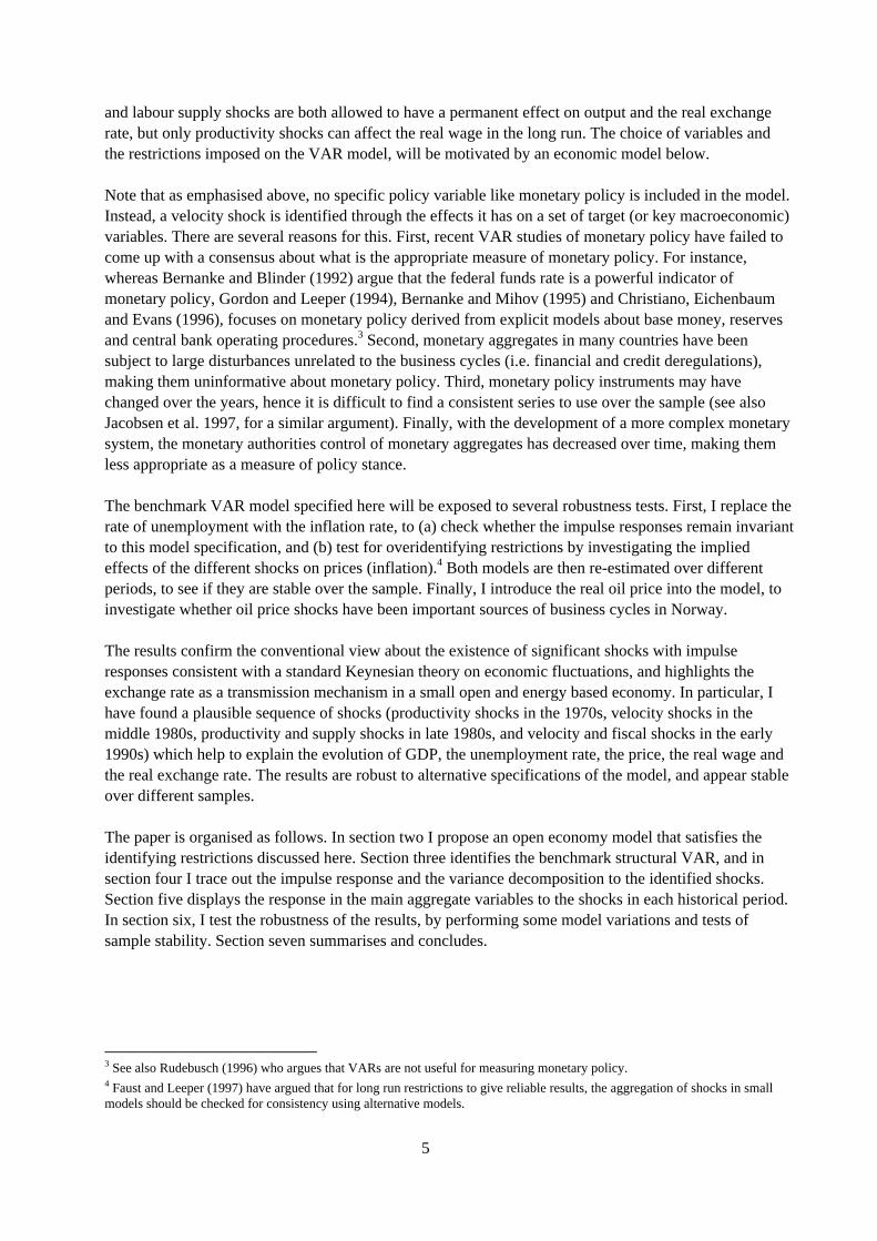
Figure 5A and 5B plot the time paths of GDP that is due to velocity and fiscal shocks respectively(setting all other shocks to zero). In figure 5C, the time path of GDP that is due to the joint (permanent)effect of the productivity and labour supply shocks, adding the drift term (also referred to as the “supplypotential”), is plotted together with the log of actual GDP. To also emphasise the short term effects of the“permanent” shocks, in figure 5D and 5E I graph the forecast error in GDP that is due to a productivityand labour supply shock respectively (together with the total forecast error in GDP), using an eightquarters weighted average of the estimated shocks. Figure 6A and 6B show the rate of unemploymenttogether with the time paths of productivity and labour supply shocks respectively over the whole period,whereas figure 6C and 6D show the rate of unemployment together with the velocity and fiscalcomponent, concentrating on the periods 1973-1987. Finally, in figure 6E, the velocity and fiscalcomponents are graphed together with the unemployment rate over the period 1989-1994.

During the 1970s, Norway experienced higher growth rates than most OECD countries. This favourableeconomic performance has usually been attributed to the discovery and use of energy resources, whichincreased productivity and stimulated the economy so it grew at a much faster rate than otherwise wouldhave been possible. This is supported in figure 5D, where the main factors behind the high growth ratesare positive productivity shocks. These results are also consistent with the results in Bjørnland (1996),where I found that aggregate supply (the joint effect of labour supply and productivity), accounted for thehigh growth rates in the 1970s. Real wages were increasing rapidly in this period (hence the positiveeffect of productivity on real wages in figure 3). The rate of unemployment is generally very low in the1970s, allowing for real wages to increase to the extent they did. By 1978, the adjustment period is over.However, aggregate demand is still high, and positive velocity and fiscal shocks contribute so that outputlies about the supply potential and unemployment falls until the early 1980s.

Norway experienced two severe recessions during the 1980s. In Bjørnland (1996), I found that whereasthe first recession was mainly “demand” driven, the second (and most severe) recession was clearly“supply” driven. Having diversified the shocks here, the main conclusions still prevail. The firstrecession from 1982 to 1985, is primarily explained by negative velocity shocks, pushing output belowthe supply potential. Fiscal shocks have also small negative effects on the real economy, and togetherwith the negative velocity shocks, they are the main factors behind the increase in the unemployment ratein this period (see figure 6C and 6D). On the other hand, labour supply shocks contribute positively tooutput growth throughout all of this period due to among other thing the increases in the femaleparticipation rate.

17

Figure 5. Components of GDP, (1975-1994)

A) Velocity, pct. change B) Fiscal, pct. change

-5

-4

-3

-2

-1

0

1

2

3

4

5

75:1 77:1 79:1 81:1 83:1 85:1 87:1 89:1 91:1 93:1

-1.5

-1

-0.5

0

0.5

1

1.5

75:1 77:1 79:1 81:1 83:1 85:1 87:1 89:1 91:1 93:1

C) Productivity and labour supply, (drift term added)

1 3 . 7

1 3 . 8

1 3 . 9

1 4

1 4 . 1

1 4 . 2

1 4 . 3

7 5 : 1 7 7 : 1 7 9 : 1 8 1 : 1 8 3 : 1 8 5 : 1 8 7 : 1 8 9 : 1 9 1 : 1 9 3 : 1

P R + L SG D P

D) Productivity, pct. change E) Labour supply, pct. change(forecast error decomposition) (forecast error decomposition)

-8

-6

-4

-2

0

2

4

6

8

10

75:1 77:1 79:1 81:1 83:1 85:1 87:1 89:1 91:1 93:1

PRTOTAL

-8

-6

-4

-2

0

2

4

6

8

10

75:1 77:1 79:1 81:1 83:1 85:1 87:1 89:1 91:1 93:1

LSTOTAL

The economy thereafter experiences a demand driven boom, set off primarily from the financialderegulation in 1984/1985. All shocks contribute positively towards output in this period (especiallyvelocity), increasing both GDP and the supply potential. However, from 1988 the spending boom inNorway accumulates in a severe financial crisis. GDP is falling and now the rate of unemployment isrising drastically. This recession is at first driven by negative productivity shocks (cf. figure 5D), andeventually negative labour supply shocks (cf. figure 5E), so that the supply potential shifts down withGDP in 1988 (cf. figure 5C). The time of the fall in the supply potential in GDP, corresponds well withthe upward shift in the rate of unemployment in 1988. The economy recovers somewhat by 1990, but by

18

that time the international economy is slowing down, and velocity shocks contribute negatively to outputgrowth until 1993. The rise in unemployment in this period is also mainly due to the negative velocityshocks.

Is it plausible to interpret the different shocks as I have done here? From the analysis above, productivityand labour supply shocks seem to fit well with the actual events that occurred in the Norwegianeconomy. Interpreting the velocity shocks as some form of monetary stance suggests in particular thatmonetary policy was loose in 1986-1987, tight from 1990-1992 and loose thereafter (c.f. figure 5A).

Figure 6. Components of Unemployment:

A) Productivity, (1975-1994) B) Labour supply, (1975-1994)

1

2

3

4

5

6

7

75:1 77:1 79:1 81:1 83:1 85:1 87:1 89:1 91:1 93:1

UnemploymentPR

1

2

3

4

5

6

7

75:1 77:1 79:1 81:1 83:1 85:1 87:1 89:1 91:1 93:1

UnemploymentLS

C) Velocity, (1975-1987) D) Fiscal, (1975-1987)

1

1.5

2

2.5

3

3.5

4

75:1 77:1 79:1 81:1 83:1 85:1 87:1

UnemploymentVEL

1

1.5

2

2.5

3

3.5

4

75:1 77:1 79:1 81:1 83:1 85:1 87:1

UnemploymentFI

E) Velocity and Fiscal, (1989-1994)

4

4 . 5

5

5 . 5

6

6 . 5

8 9 : 1 9 0 : 1 9 1 : 1 9 2 : 1 9 3 : 1 9 4 : 1

U n e m p lo y m e n tF IV E L

19

A similar stance of monetary policy is suggested using a simple monetary conditions index (MCI), thatrelates changes in interest rates and the real exchange rate to aggregate demand (even when we allow foruncertainty with regard to for instance dynamics, cointegration and parameter constancy), (see Eika et al.1996).

The effects of the “fiscal” shocks are more difficult to interpret as the impact on GDP is small. Howeverthe fiscal shocks can be better understood by analysing the unemployment rate, and as suggested above,fiscal shocks may have captured a part of fiscal policies aimed at achieving full employment. In Norway,a period of expansionary fiscal polices ended in 1982. Except for a brief period in 1985-1986, fiscalpolices remained tight throughout the 1980s, especially in 1988-1989, but was again expansionary from1990 to 1993. During the periods of tight fiscal polices, output falls somewhat, but unemployment isclearly worsened (c.f. figure 5B and 6D). The expansionary fiscal policies in the mid-1980s and from1990, increase output and work to reduce the unemployment rate, especially from 1990s (see figure 6E).These results emphasise that to the extent that fiscal shocks have captured the effects of fiscal polices,fiscal polices have been used countercyclically from the late 1980s, (see also Holden 1997, for similarconclusions).

Finally, what are the responses of the real exchange rate to the different shocks? Since the collapse of theBretton Woods system of fixed exchange rates in 1971, the Norwegian currency has participated inseveral exchange rate systems, some more flexible than others (see Norges Bank 1995). Figure7A-C give the time path of the real exchange rate to the three most important shocks; Productivity,velocity and fiscal shocks respectively (drift term added for productivity and fiscal shocks). To alsoemphasise the short term effects of the fiscal shock, figure 7D shows the forecast error in real exchangerate that is due to the fiscal shocks, together with the total forecast error.

The positive productivity shocks in the 1970s clearly worked to appreciate the real exchange rate,whereas the negative productivity shocks from 1987 and onwards, work to depreciate the real exchangerate. Negative velocity shocks in the recession in the early 1980s appreciate the real exchange rate,whereas in the boom from 1984, the real exchange rate depreciates. From 1990, the negative velocityshocks (that reduces output) also appreciates the real exchange rate.

Expansionary fiscal polices in the late 1970s, some periods in the 1980s and in the early 1990s appreciatethe real exchange rate, whereas tight fiscal policies from 1982 and in particular from 1988-1989depreciate the real exchange rate (cf. figure 7D). However, the large importance of fiscal shocks inexplaining real exchange rate movements, suggests that the “fiscal shocks” identified here have alsocaptured the exchange rate instruments used in this period. This can be explained as follows. During the1970s and the 1980s, expansionary fiscal policies brought with them higher inflation, thereby anappreciated real exchange rate, reduced competitiveness, a current account deficit and eventually,increasing unemployment. An important part of economic policy in this period was then to devaluate theexchange rate each time competitiveness was low (see Norges Bank 1995, and Bowitz and Hove 1996).

The implied responses of the real exchange rate and the unemployment rate to a fiscal shock reported infigure 2 are consistent with this scenario. Expansionary fiscal polices reduce the unemployment rate atfirst, but eventually, unemployment starts to increase. The major currency devaluations in 1977Q3,1978Q1, 1982Q3, 1982Q4 and 1984Q3 all followed after periods of increasing unemployment rates.However, the unemployment rate reacts with a lag to the exchange rate changes so that a depreciation atfirst increases the rate of unemployment, before after three quarters, unemployment starts to fall (cf.figure 2). The currency devaluations can be seen as positive fiscal shocks in figure 7D, and within threequarters of each of the fiscal shocks, the rate of unemployment starts to drop (see figure 6D).

20

6. Extension of the benchmark modelTo analyse the robustness of the results reported so far, I alter the benchmark model in several ways.First, Faust and Leeper (1997) have criticised the use of long run restrictions to identify structuralshocks, and show that unless the economy satisfies some types of strong restrictions, the long runrestrictions will be unreliable. In particular they argue that for the long run restrictions to give reliableresults, the aggregation of shocks in small models should be checked for consistency using alternativemodels.12 For instance, as the model presented in section two could have been solved for the growth rateof prices rather than for the unemployment rate, I replace the unemployment rate with inflation and re-estimate the model (denoted inflation model). This allows us to check whether the impulse responsesremain invariant to this new model specifications. In addition, I can test for overidentifying restrictionsby investigating whether the implied price response is consistent with the theoretical model presented insection two. Both the benchmark and the inflation model are thereafter re-estimated over differentperiods, to see if they are stable over the sample. Finally, I introduce the real price of oil into the VARmodel, to investigate whether oil price shocks are important sources behind the economic fluctuations inNorway. In particular, I want to check whether the rise in the oil price throughout the 1970s can account

12 Strictly speaking, Faust and Leeper’s (1997) critique of the use of long run restrictions in VAR models refers to a bivariatemodel using only one long run restriction like that of Blanchard and Quah (1989), where the problem stems from the fact that theunderlying model has more sources of shocks (with sufficiently different dynamic effects on the variables considered) than doesthe estimated model. In that case, the bivariate model can be misspecified and the associated decomposition and impulseresponses of little use. The fact that we here allow for more variables and use several long run restrictions together, may by itselfbe sufficient to side step this criticism.

Figure 7. Components of the real exchange rate, (1975-1994)

A) Productivity, (drift term added) B) Velocity, pct. change

4.3

4.35

4.4

4.45

4.5

4.55

75:1 77:1 79:1 81:1 83:1 85:1 87:1 89:1 91:1 93:1

PRReal exchange rate

-2

-1.5

-1

-0.5

0

0.5

1

1.5

2

75:1 77:1 79:1 81:1 83:1 85:1 87:1 89:1 91:1 93:1

C) Fiscal, (drift term added) D) Fiscal, pct. change(forecast error decomposition)

4.25

4.3

4.35

4.4

4.45

4.5

4.55

4.6

75:1 77:1 79:1 81:1 83:1 85:1 87:1 89:1 91:1 93:1

FIReal exchange rate

-10

-5

0

5

10

15

75:1 77:1 79:1 81:1 83:1 85:1 87:1 89:1 91:1 93:1

FITOTAL

21

for the real exchange rate appreciation already captured by the productivity shocks. The answer to thisquestion is no.

6.1. A model containing prices

By solving the model described in section two for the growth rate in prices, I can find the implied effectof each of the four shocks on the price level:

(12’) ∆pt tVEL

tFI

tPR

tPR

tLS= + + − + − + − −− − − −ε βπ ε ε α γ βδ ε βσ ε1 1 1 11 1( ) ( ) ( )

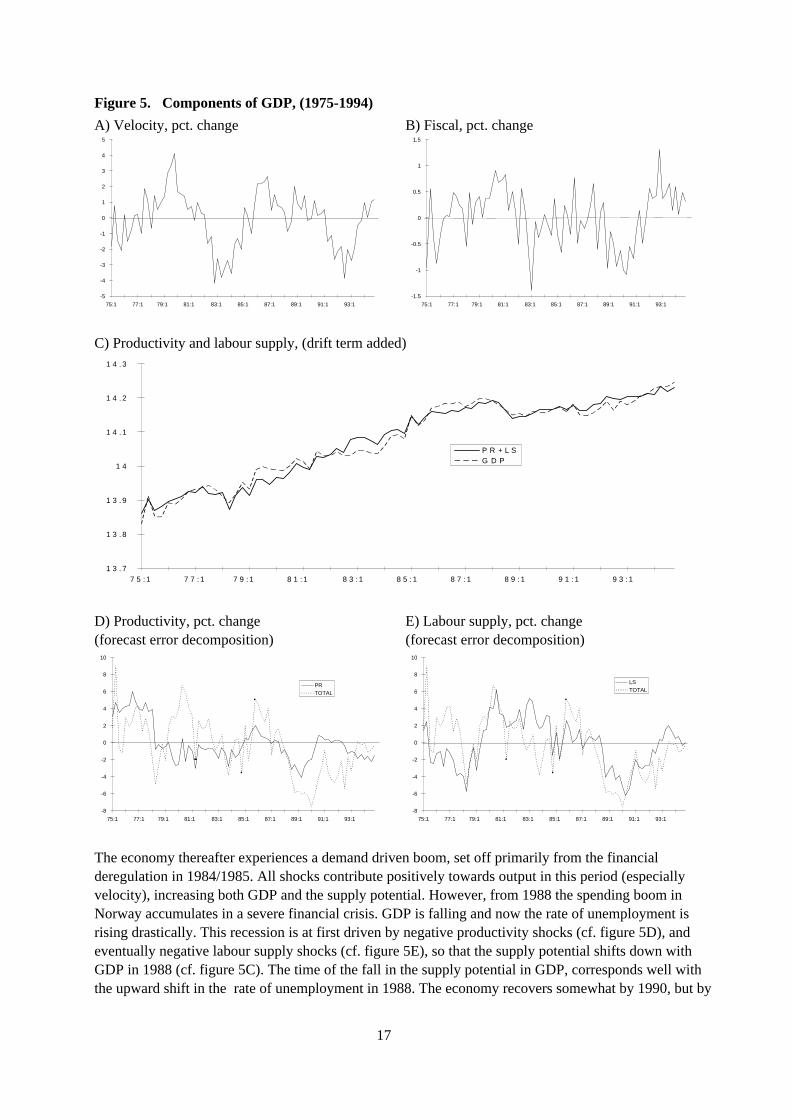
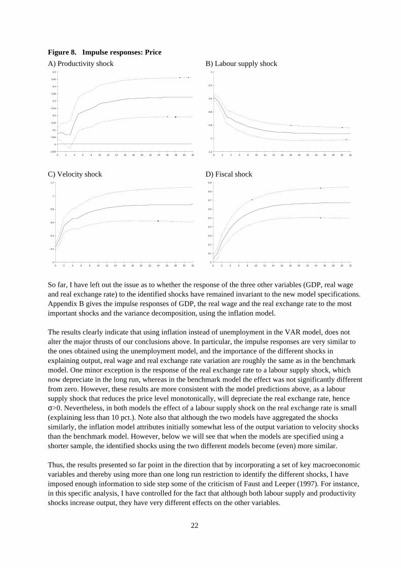
Equation (12’) suggests a set of overidentifying restrictions. First, all shocks can have a permanent effecton the price, (although none of the shocks will have a long run effect on inflation if it is stationary). Avelocity shock will increase the price level after a period, whereas the effect of the fiscal shock ispositive if (βπ>-1). Following a productivity shock, the price level will fall immediately, although thelong run effect may be both positive or negative (recall that we expect δ<0). A labour supply shockreduces the price level directly (although the effect may be somewhat offset if the exchange ratedepreciates).

To measure prices, I use the CPI as it is calculated independently of output volume. The CPI seems to bein the borderline between being an I(1) or an I(2) variable. Although I can reject the hypothesis thatinflation is I(1) against the trend stationary alternative at the 5 pct. level (ADF = -3.64), all evidence ofI(1) in inflation disappeared once a structural break in 1988Q2 was removed from the inflation rate (cf.Bjørnland 1995). In fact, this is the same period I found a structural break in the unemployment rate. Inthe remaining analysis I therefore include a dummy that is one from 1988Q2 an onwards in the inflationrate.13 An intervention dummy that is 1 in 1979Q1 but zero otherwise, is also included in the inflationequation to reflect the price stop in that period. To be consistent with the benchmark model, the VARcontains four lags and an intervention dummy for 1973 in the equation for the real exchange rate. Withfour lags, the model satisfies tests of autocorrelation, heteroscedasticity and non-normality (see tableA.5). Finally, the variables will be estimated in difference form, as there is no evidence of cointegrationbetween the level of the variables (see table A.8).

Figures 8A-8D report the cumulative response in the price to a one unit velocity shock, fiscal shock,productivity shock and labour supply shock respectively, with a one standard error band around the pointestimates. Clearly, the response in the price is consistent with the model predictions above and satisfy theoveridentifying restrictions. The price increases gradually with both velocity and fiscal shocks, and theeffect is not stabilised before after three years, where the (unit) velocity shock has increased the pricelevel by 0.8-1 percentage. Note that the response to the velocity shock is consistent with the conventionalidea of how a monetary shock works. In particular, contrary to many VAR studies incorporatingmonetary policy explicitly, I avoid the so-called price puzzle, where the price increases following acontractionary monetary policy (see Sims 1992, and Leeper et. al. 1996). The effect of a productivityshock is small and approaching zero the first year, but then increases somewhat and is significantlydifferent from zero in the long run. Labour supply shocks reduce the price level monotonically asexpected.

13 An alternative would be to use a trend in the inflation rate. However, once the dummy is included, the trend is no longer issignificant. Further, prior and post 1988, we can reject the unit root in inflation in favour of the stationary alternative.

22

So far, I have left out the issue as to whether the response of the three other variables (GDP, real wageand real exchange rate) to the identified shocks have remained invariant to the new model specifications.Appendix B gives the impulse responses of GDP, the real wage and the real exchange rate to the mostimportant shocks and the variance decomposition, using the inflation model.

The results clearly indicate that using inflation instead of unemployment in the VAR model, does notalter the major thrusts of our conclusions above. In particular, the impulse responses are very similar tothe ones obtained using the unemployment model, and the importance of the different shocks inexplaining output, real wage and real exchange rate variation are roughly the same as in the benchmarkmodel. One minor exception is the response of the real exchange rate to a labour supply shock, whichnow depreciate in the long run, whereas in the benchmark model the effect was not significantly differentfrom zero. However, these results are more consistent with the model predictions above, as a laboursupply shock that reduces the price level monotonically, will depreciate the real exchange rate, henceσ>0. Nevertheless, in both models the effect of a labour supply shock on the real exchange rate is small(explaining less than 10 pct.). Note also that although the two models have aggregated the shockssimilarly, the inflation model attributes initially somewhat less of the output variation to velocity shocksthan the benchmark model. However, below we will see that when the models are specified using ashorter sample, the identified shocks using the two different models become (even) more similar.

Thus, the results presented so far point in the direction that by incorporating a set of key macroeconomicvariables and thereby using more than one long run restriction to identify the different shocks, I haveimposed enough information to side step some of the criticism of Faust and Leeper (1997). For instance,in this specific analysis, I have controlled for the fact that although both labour supply and productivityshocks increase output, they have very different effects on the other variables.

Figure 8. Impulse responses: Price

A) Productivity shock B) Labour supply shock

-0.05

0

0.05

0.1

0.15

0.2

0.25

0.3

0.35

0.4

0.45

0.5

0 2 4 6 8 10 12 14 16 18 20 22 24 26 28 30 32 -1.2

-1

-0.8

-0.6

-0.4

-0.2

0

0 2 4 6 8 10 12 14 16 18 20 22 24 26 28 30 32

C) Velocity shock D) Fiscal shock

0

0.2

0.4

0.6

0.8

1

1.2

0 2 4 6 8 10 12 14 16 18 20 22 24 26 28 30 32 0

0.1

0.2

0.3

0.4

0.5

0.6

0.7

0.8

0.9

0 2 4 6 8 10 12 14 16 18 20 22 24 26 28 30 32

23

6.2. Sample stability

Both the benchmark and the inflation model are re-estimated using the sample 1973-1987. 1987 is chosenas the end date, as both unemployment and inflation experienced a structural break in 1988.14 Overall, theresults reported above are strengthened by focusing on the period 1973-1987. In particular, the impulseresponses and the variance decompositions indicate that using the smaller sample generates very muchthe same results as when the full sample was used (see appendix C). One exception is the response ofoutput and the real exchange rate to a productivity shock, where the variance decomposition using bothmodels attribute less off the output fluctuations and more of the real exchange rate fluctuations to aproductivity shock than when the full sample was used. However, as the benchmark and the inflationmodel are consistent with each other, the results indicate that I have underestimated the importance of theproductivity shocks by focusing only on the period until 1987, as was seen above, productivity shocksplay an important role in the recession from 1988 and onwards. Note that now both models attributeapproximately the same share of output variation to velocity shocks.

6.3. The role of oil price

The two oil price shocks of the 1970s are thought to have had important roles in explaining periods ofglobal recession and inflation, and are therefore the typical textbook examples of adverse supply shocks.Norway is in a special position as it discovered oil in the North sea in the early 1970s, and was anexporter of oil before the oil price shock in the late 1970s. Previous studies of the effects of a real oilprice shock on the mainland economy has emphasised that Norway has actually gained from a higher realoil price (by increasing net wealth and demand), and consequently, suffered when the real oil price waslow (see e.g. Bjørnland 1996).

In this section I include the real oil price into the model to specifically investigate the effects of oil priceshocks on the mainland economy. The model allows for a more complex set of possible channels ofinfluence than in Bjørnland (1996). In particular, I can now control for the possibility that the exchangerate may be a “petrocurrency”, that appreciates when the oil price is high and depreciates when the oilprice is low. For instance, Haldane (1997) has argued that the rise in oil prices can explain a large part ofthe appreciated Norwegian currency. Incorporating oil prices into both models also serves as a check onwhether the established effects of the other shocks remain the same.

In appendix D, the model reported in section two is augmented to allow for the influence of the real oilprice. Solving the model, the oil price shock is identified as the only shock that can have a long run effecton the real oil price. However, no restrictions are placed on the response of the other variables to the oilprice shocks. The impulse responses of an oil price shock using the benchmark model is presented infigure 9, while the variance decompositions for all shocks are presented in appendix E. The impulseresponses of an oil price shocks using the inflation model are also presented in appendix E forcomparisons.15

14 Using the period 1973-1987, we can reject the hypothesis of an unit root in favour of the stationary alternative for inflation butnot for unemployment. However, there is evidence that we can reject the unit root hypothesis in unemployment, using a trendinstead. Hence, we include a trend in the unemployment rate (it comes out significant). Both models satisfy tests ofautocorrelation, heteroscedasticity and non-normality at the 5 percentage level, and none of the variables are cointegrated (see theresults using the benchmark model in table A.6 and A.9).15 I can not reject the hypothesis of a unit root in the real oil price, but its first differences are stationary. There is no evidencethat the oil price is cointegrating with the other variables. Four lags are used in the VAR model to be consistent with thebenchmark model. An additional three intervention dummies are included into the equation for oil prices to take care of theextreme outliers (see figure A.1). The first dummy is 1 in 1974Q1 but zero otherwise, the second dummy is 1 in 1986Q1 but zerootherwise, while the third dummy is 1 in 1990Q3, -1 but 1991Q1 and zero otherwise.

24

The results support the findings reported in Bjørnland (1996). In particular, the benchmark and theinflation models are consistent with each other, and suggest that an oil price shock increases GDPpermanently. However, the standard deviation bands are wide indicating that the long run effect is notsignificant. Unemployment increases temporarily, indicating that although a real oil price shockstimulates the economy (so employment increases in some sectors) some workers are laid off in othersectors so total unemployment rises.

Figure 9. Impulse response to an oil price shock using the benchmark model

A) Real GDP B) Unemployment

-0.6

-0.4

-0.2

0

0.2

0.4

0.6

0.8

1

1.2

1.4

0 2 4 6 8 10 12 14 16 18 20 22 24 26 28 30 32-0.08

-0.06

-0.04

-0.02

0

0.02

0.04

0.06

0.08

0.1

0 2 4 6 8 10 12 14 16 18 20 22 24 26 28 30 32

C) Real exchange rate D) Real wage

-0.6

-0.4

-0.2

0

0.2

0.4

0.6

0.8

0 2 4 6 8 10 12 14 16 18 20 22 24 26 28 30 32-0.4

-0.3

-0.2

-0.1

0

0.1

0.2

0.3

0.4

0.5

0.6

0.7

0 2 4 6 8 10 12 14 16 18 20 22 24 26 28 30 32

Using the inflation model, we find that the an oil price shock has initially no effect on the price level, butafter a year, the price has increased and is significant different from zero (see appendix E). That an oilprice shock affects the Norwegian inflation rates with a lag was also found in Bjørnland (1997). The realexchange rate depreciates the first two quarters following an oil price shock, but thereafter appreciatesback towards equilibrium (or just below equilibrium), where the effect is no longer significant. Theinitial deprecation of the real exchange rate to an oil price shock is consistent with the fact that thedomestic price level reacts slowly to an oil price increase, while foreign prices rise immediately to thesame shock. The domestic price eventually starts to increase, and consistent with this scenario, the realexchange rate appreciates back to equilibrium.16 Finally, the effect of an oil price shock on the real wageis not significant different from zero.

16 These results are independent of whether we use a nominal or real oil price, or whether the nominal oil price is denoted in USdollar or in Norwegian kroner.

25

The variance decompositions emphasise that a real oil price shock explains about 10-15 pct of the outputvariation, 3-5 pct. of the unemployment variation, the price variation and the real exchange rate variation,and 0-3 pct. of the real wage variation. The responses in the different variables to the other shocks(productivity, labour supply, fiscal and velocity shocks) remain invariant to the inclusion of oil pricesinto the models, except that the labour supply and the productivity shock now explains somewhat less ofthe variation in GDP than previously.

To conclude, I have found no evidence to support Haldane’s (1997) claim that the oil price increasesexplain a large part of the Norwegian real exchange rate appreciation. Similar conclusions have also beenmade in Aliber, (1990) and the references cited there. On the other hand, the oil price shocks explainmore of the variation in GDP, and analysis in sub samples suggest that the effect is most importantduring the periods 1973/1974, 1979/1980 and 1986, (corresponding approximately to the three largest oilprice shocks).

7. Conclusions and summaryIn this paper, I have focused on the relative ability of real and nominal shocks to explain business cyclesin a small open, energy rich country like Norway. To do so I have specified a structural VAR model inGDP, the real wage, the real exchange rate and the rate of unemployment (or price), that is identifiedthrough long run restrictions on the dynamic multipliers in the model. The way the model is specified, Iidentify four structural shocks; Velocity, fiscal, productivity and labour supply shocks. The model is alsoaugmented to allow for oil price shocks.

The results indicate that I have found a plausible sequence of shocks (productivity shocks in the 1970s,velocity shocks in the middle 1980s, productivity and labour supply shocks in the late 1980s, andvelocity and fiscal shocks in the early 1990s) which help to explain the evolution of real GDP,unemployment, CPI, the real wage and the real exchange rate the last two decades.

The identified shocks are consistent with standard Keynesian theory on economic fluctuations. Inparticular, following a velocity and a fiscal shock, GDP increases and unemployment falls temporarily,while prices increase gradually and permanently. However, whereas a velocity shock depreciates the realexchange rate before it overshoots back to equilibrium, the fiscal shock has a long run appreciation effecton the real exchange rate. Both productivity and labour supply shocks have a long run positive effect onGDP, but the effects on the other variables differs. In particular, whereas a favourable productivity shockreduces unemployment (and increases the price), a favourable labour supply shock increasesunemployment (and reduces the price). A productivity shock increases the real wage permanently and hasa long run appreciation effect on the real exchange rate.

The results highlight the exchange rate as a transmission mechanism in a small open and energy basedeconomy. In particular, the response in the real exchange rate to a productivity shock is consistent withthe fact that Norway is a resource rich country, where the energy discoveries have given rise toproductivity and wealth effects that have appreciated the exchange rate. Augmenting the model to allowfor oil prices do not change this conclusion, and oil price shocks have had little explanatory power for thereal exchange rate developments. These findings are robust to alternative specifications of the model andare stable over the sample.

Although most of the shocks are well interpreted in terms of the actual episodes that have occurred in theperiods examined, further work may be needed in particular to validate the interpretations of the “fiscal

26

shocks” as those that represent fiscal and exchange rate polices. In particular, as one importantmotivation for the government to use exchange rate polices throughout the 1970s and 1980s was tostabilise the current account, this suggest that one possible extension of the model could be to investigatethe implied effects of the fiscal shocks on the current account. Preliminary results suggest that fiscalshocks do improve the current account, but as was also found in Bowitz and Hove (1996), the effect issmall and the main improvement of the current account comes through other channels.

27

ReferencesAliber, R.Z. (1990): “Exchange Rate Arrangements”, in D.T. Llewellyn and C. Milner (eds.): CurrentIssues in International Monetary Economics, London: Macmillan Education LTD, 196-212.

Balassa, B. (1964): The Purchasing Power Parity Doctrine: A Reappraisal, Journal of Political Economy,72, 584-596.

Bernanke, B.S. and A.S. Blinder (1992): The Federal Funds Rate and the Channels of MonetaryTransmission, American Economic Review, 82, 901-22.

Bernanke B.S. and I. Mihov (1995): Measuring Monetary Policy, NBER Working paper 5145, NationalBureau of Economic Research.

Bjørnland, H. C. (1995): Trends, Cycles and Measures of Persistence in the Norwegian Economy, Socialand Economic Studies 92, Statistics Norway.

Bjørnland, H.C. (1996): The Dynamic Effects of Aggregate Demand, Supply and Oil Price Shocks,Discussion Papers 174, Statistics Norway.

Bjørnland, H.C. (1997): Estimating Core Inflation-The Role of Oil Price Shocks and Imported Inflation,Discussion Papers 200, Statistics Norway.

Blanchard, O. (1997): Is There a Core of Usable Macroeconomics?, American Economic Review Papersand Proceedings, 87, 2440-246.

Blanchard, O. and D. Quah (1989): The Dynamic Effects of Aggregate Demand and SupplyDisturbances, American Economic Review, 79, 655-673

Blanchard, O.J and D. Quah (1993): Fundamentalness and the interpretation of time series evidence:Reply to Lippi and Reichlin, American Economic review, 83, 653-658.

Blinder, A.S. (1997): Is There a Core of Practical Macroeconomics That We Should All Believe?,American Economic Review Papers and Proceedings, 87, 240-243.

Bowitz, E. and S.I. Hove (1996): Business cycles and fiscal policy: Norway 1973-93, Discussion Papers178, Statistics Norway.

Christiano, L.J., M. Eichenbaum and C. Evans (1996): The Effects of Monetary Policy Shocks: Evidenceform the Flow of Funds, Review of Economics and Statistics, 53, 16-34.

Clarida, R. and J. Gali (1994): Sources of Real Exchange Rate Fluctuations: How Important are NominalShocks?, NBER Working Paper No. 4658.

Corden, W.M. and J.P. Neary (1982): Booming Sector and De-industrialisation in a small OpenEconomy, Economic Journal, 92, 825-848.

Cushman, D.O. and T. Zha (1997): Identifying monetary policy in a small open economy under flexibleexchange rates, Journal of Monetary Economics, 39. 433-448.

28

Dolado, J.J. and J.D. López-Salido (1996): Hysteresis and Economic Fluctuations (Spain, 1970-1994),CEPR Discussion Paper no. 1334.

Doornik, J.A. and D.F. Hendry (1994): PcFiml 8.0. Interactive Econometric Modelling of DynamicSystems, London: International Thomson Publishing.

Dornbusch, R. (1976): Expectations and exchange rate dynamics, Journal of Political Economy, 84,1167-1176.

Eichenbaum, M. (1997): Is There a Core of Practical Macroeconomics? Some Thoughts on PracticalStabilization Policy, American Economic Review Papers and Proceedings, 87, 236-239.

Eika, K.H., N.R. Ericsson and R. Nymoen (1996): Hazards in implementing a monetary conditions index,Working Paper 1996/9, Norges Bank.

Engle, R. (1982). Autoregressive Conditional Heteroscedasticity with Estimates of the Variance ofUnited Kingdom inflation, Econometrica, 50, 987-1008.

Faust, J. and E.M. Leeper (1997): When Do Long-Run Identifying Restrictions Give Reliable Results?,Journal of Business and Economic Statistics, 15, 345-353.

Fischer, S. (1977): Long-Term Contracts, Rational Expectations, and the Optimal Money Supply Rule,Journal of Political Economy, 85, 191-205.

Gamber, E.N. and F. L. Joutz (1993): The Dynamic Effects of Aggregate Demand and SupplyDisturbances: Comment, American Economic Review, 83, 1387-1393.

Gordon, D.B. and E.M. Leeper (1994): The Dynamic Impacts of Monetary Policy: An Excise inTentative Identification, Journal of Political Economy, 102, 1228-1247.

Haldane, A.G. (1997): The Monetary Framework in Norway, unpublished manuscript, Bank of England.

Holden, S. (1997): The Unemployment problem - A Norwegian Perspective, OECD, EconomicDepartment Working Papers No. 172.

Jacobsen, T., P. Jansson, A, Vredin, and A. Warne (1997): A VAR model for Monetary Policy Analysisin a Small Open Economy, unpublished manuscript.

Johansen, S. (1988): Statistical Analysis of Cointegrating Vectors, Journal of Economic Dynamics andControl, 12, 231-254.

Johansen, S. (1991): Estimation and Hypothesis Testing of Cointegration Vectors in Gaussian VectorAutoregressive Models, Econometrica, 59, 1551-1580.

Kydland, F.E. and E.C. Prescott (1982): Time To Build and Aggregate Fluctuations, Econometrica, 50,1345-70

Leeper, E.M., C.A. Sims and T. Zha (1996): What does monetary policy do?, Brookings Papers onEconomic activity, 2, 1-78.

29

Lippi, M. and L. Reichlin (1993): A note on measuring the dynamic effects of aggregate demand andaggregate supply disturbances, American Economic Review, 83, 644-652.

Norges Bank (1995): Norske Finansmarkeder, Norsk Penge-og Valutapolitikk, Norges Bank Skrifteserieno. 23

Osterwald-Lenum, M (1992). A Note with Quantiles of the Asymptotic Distribution of the MaximumLikelihood Cointegration Rank Test Statistics, Oxford Bulletin of Economics and Statistics 54, 461-471.

Phelps, E.S. and J.B. Taylor (1977): Stabilizing powers of monetary policy under rational expectations,Journal of Political Economy, 85, 163-190.

Reimers, H.-E. (1992) Comparisons of tests for multivariate cointegration, Statistical Papers, 33,335-359.

Rogoff, K. (1996): The Purchasing Power Parity Puzzle, Journal of Economic Literature, 34,647-668.

Rudebusch, G.D. (1996): Do Measures of Monetary Policy in a VAR Make Sense?, unpublishedmanuscript.

Samuelson, P. (1964): Theoretical Notes on Trade Problems, Review of Economic Statistics, 46,145-154.

Serletis, A. and G. Zimonopoulos (1997): Breaking Trend Functions in Real Exchange Rates: Evidencefrom Seventeen OECD Countries, Journal of Macroeconomics, 19, 781-802.

Sims, C.A. (1992): Interpreting the macroeconomic time series facts: the effects of monetary policy,European Economic Review, 36, 975-1000.

Solow, R.M. (1997): Is There a Core of Usable Macroeconomics We Should All Believe In?, AmericanEconomic Review Papers and Proceedings, 87, 230-232.

Taylor, J.B. (1997): A Core of Usable Macroeconomics, American Economic Review Papers andProceedings, 87, 233-235.

Yun, T. (1996): Nominal price rigidity, money supply endogeneity and business cycles, Journal ofMonetary Economics, 37, 345-370.

Zivot, E and D.W. K. Andrews (1992): Further Evidence on the Great Crash, the Oil-Price Shock, andthe Unit-Root Hypothesis, Journal of Business and Economic Statistics, 10, 251-270.

30

Appendix A. Data and model specifications

Figure A.1. Plots of the data series

A) Log GDP B) Log real wage C) Log real exchange rate

13.6

13.7

13.8

13.9

14

14.1

14.2

14.3

72:1 74:1 76:1 78:1 80:1 82:1 84:1 86:1 88:1 90:1 92:1 94:1 4.2

4.3

4.4

4.5

4.6

4.7

4.8

4.9

72:1 74:1 76:1 78:1 80:1 82:1 84:1 86:1 88:1 90:1 92:1 94:1

4.25

4.3

4.35

4.4

4.45

4.5

4.55

4.6

72:1 74:1 76:1 78:1 80:1 82:1 84:1 86:1 88:1 90:1 92:1 94:1

C) First differences of log D) First differences of log E) First differences of logGDP Real wage Real exchange rate

-0.08

-0.06

-0.04

-0.02

0

0.02

0.04

0.06

0.08

0.1

72:1 74:1 76:1 78:1 80:1 82:1 84:1 86:1 88:1 90:1 92:1 94:1 -0.06

-0.04

-0.02

0

0.02

0.04

0.06

0.08

72:1 74:1 76:1 78:1 80:1 82:1 84:1 86:1 88:1 90:1 92:1 94:1 -0.06

-0.05

-0.04

-0.03

-0.02

-0.01

0

0.01

0.02

0.03

0.04

72:1 74:1 76:1 78:1 80:1 82:1 84:1 86:1 88:1 90:1 92:1 94:1

F) Log CPI G) Log real oil price H) Unemployment rate

-1.6

-1.4

-1.2

-1

-0.8

-0.6

-0.4

-0.2

0

0.2

72:1 74:1 76:1 78:1 80:1 82:1 84:1 86:1 88:1 90:1 92:1 94:1 3.5

4

4.5

5

5.5

6

6.5

72:1 74:1 76:1 78:1 80:1 82:1 84:1 86:1 88:1 90:1 92:1 94:1 0

1

2

3

4

5

6

7

72:1 74:1 76:1 78:1 80:1 82:1 84:1 86:1 88:1 90:1 92:1 94:1

I) First differences of log J) First differences of logCPI Real oil price

-0.01

0

0.01

0.02

0.03

0.04

0.05

72:1 74:1 76:1 78:1 80:1 82:1 84:1 86:1 88:1 90:1 92:1 94:1 -0.8

-0.6

-0.4

-0.2

0

0.2

0.4

0.6

0.8

1

72:1 74:1 76:1 78:1 80:1 82:1 84:1 86:1 88:1 90:1 92:1 94:1

31

Data sources

The sample runs from 1972Q1-1994Q4. Using first differences and four lags in the VAR, the estimationsample is 1973Q2-1994Q4. All variables except the real exchange rate and the real oil price areseasonally adjusted quarterly variables, taken from Kvarts Database, Statistics Norway. (y); GrossDomestic Product, mainland Norway (GDP less petroleum activities and ocean transport) constant 1991prices. (rw); Real wages in mainland Norway, deflated by the implicit price deflator of GDP mainlandNorway. (u); Unemployment rate. (p); Consumer price index.

The real exchange rate (s) is taken from Troll8, Norges Bank, and is the Central Bank exchange rateindex, deflated by a set of relative consumer prices. The real oil price (op) is calculated from the nominaloil price (Saudi Arabian Light-34, USD per barrel, fob- (n.s.a.). Prior to 1980, posted prices, thereafterspot prices) and deflated by the implicit GDP deflator, mainland Norway. Source: OPEC BULLETINand Statistics Norway. All variables except the unemployment rate are in logarithms.

Table A.1. Augmented Dickey-Fuller unit-root tests, 1974Q2-1994Q4

Series1 ADF(lags) tADF Series2 ADF(lags) tADF

y ADF(1) -2.01 ∆y ADF(5) -4.51***s ADF(4) -1.88 ∆s ADF(4) -4.27***rw ADF(5) -3.27 ∆rw ADF(4) -3.88***u ADF(2) -2.25 ∆u ADF(1) -5.03***1 A constant and a time trend are included in the regression2 A constant is included in the regression.** Rejection of the unit root hypothesis at the 5 percentage level*** Rejection of the unit root hypothesis at the 2.5 percentage level

Table A.2. Sequential unit-roots test 1974Q2-1994Q41

Model Period Minimum t-statisticsUnemploymentReal wagesReal exchange rateGDP

ABCA

1988Q21976Q41989Q41988Q2

-4.68*-4.01-3.34-4.08

1 Critical values were taken from Zivot and Andrews (1992, p. 256-257). Three alternative hypothesis are considered: (A) changein the level of the trend, (B) change in the growth rate of the trend, (C) change in both the level and the growth rate of the trend.* Rejection of the unit root hypothesis at the 10 percentage level

Table A.3. F-tests for model reductions1

Lags Sequential F-tests p-value Direct F-tests p-value87 F(16, 144) = 0.81 0.671 F(16, 114) = 0.81 0.6716 F(16, 156) = 0.99 0.461 F(32, 174) = 0.90 0.6295 F(16, 168) = 2.17 0.008 F(48, 183) = 1.30 0.1114 F(16, 180) = 1.27 0.220 F(64, 186) = 1.31 0.0833 F(16, 193) = 2.15 0.008 F(80, 187) = 1.51 0.0122 F(16, 205) = 1.11 0.347 F(96, 188) = 1.47 0.0131 F(16, 217) = 1.21 0.265 F(112, 189) = 1.46 0.0111 Sequential F-test with corresponding p-value reports the sequential model reductions (8→7,...,2→1 lags), direct F-test withcorresponding p-value reports the direct model reductions (8→7, ..., 8→1 lags). All test-statistics are calculated using PcFiml 8.0(see Doornik and Hendry 1994).

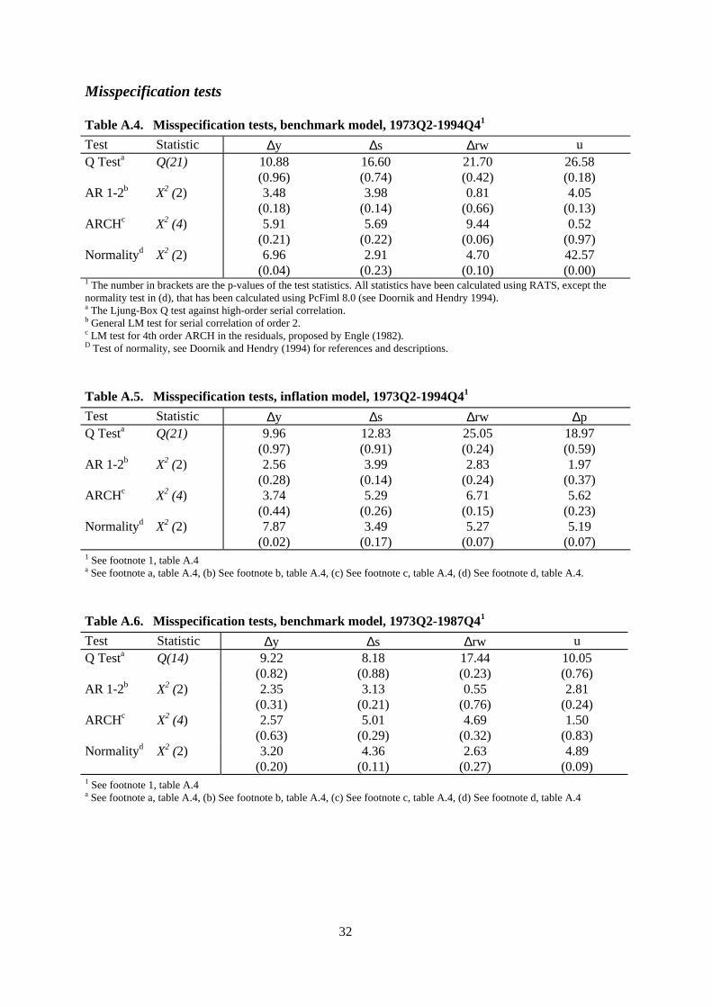
32

Misspecification tests

Table A.4. Misspecification tests, benchmark model, 1973Q2-1994Q41

Test Statistic ∆y ∆s ∆rw uQ Testa Q(21) 10.88

(0.96)16.60(0.74)

21.70(0.42)

26.58(0.18)

AR 1-2b X2 (2) 3.48(0.18)

3.98(0.14)

0.81(0.66)

4.05(0.13)

ARCHc X2 (4) 5.91(0.21)

5.69(0.22)

9.44(0.06)

0.52(0.97)

Normalityd X2 (2) 6.96(0.04)

2.91(0.23)

4.70(0.10)

42.57(0.00)

1 The number in brackets are the p-values of the test statistics. All statistics have been calculated using RATS, except thenormality test in (d), that has been calculated using PcFiml 8.0 (see Doornik and Hendry 1994).a The Ljung-Box Q test against high-order serial correlation.b General LM test for serial correlation of order 2.c LM test for 4th order ARCH in the residuals, proposed by Engle (1982).D Test of normality, see Doornik and Hendry (1994) for references and descriptions.

Table A.5. Misspecification tests, inflation model, 1973Q2-1994Q41

Test Statistic ∆y ∆s ∆rw ∆pQ Testa Q(21) 9.96

(0.97)12.83(0.91)

25.05(0.24)

18.97(0.59)

AR 1-2b X2 (2) 2.56(0.28)

3.99(0.14)

2.83(0.24)

1.97(0.37)

ARCHc X2 (4) 3.74(0.44)

5.29(0.26)

6.71(0.15)

5.62(0.23)

Normalityd X2 (2) 7.87(0.02)

3.49(0.17)

5.27(0.07)

5.19(0.07)

1 See footnote 1, table A.4a See footnote a, table A.4, (b) See footnote b, table A.4, (c) See footnote c, table A.4, (d) See footnote d, table A.4.

Table A.6. Misspecification tests, benchmark model, 1973Q2-1987Q41

Test Statistic ∆y ∆s ∆rw uQ Testa Q(14) 9.22

(0.82)8.18

(0.88)17.44(0.23)

10.05(0.76)

AR 1-2b X2 (2) 2.35(0.31)

3.13(0.21)

0.55(0.76)

2.81(0.24)

ARCHc X2 (4) 2.57(0.63)

5.01(0.29)

4.69(0.32)

1.50(0.83)

Normalityd X2 (2) 3.20(0.20)

4.36(0.11)

2.63(0.27)

4.89(0.09)

1 See footnote 1, table A.4a See footnote a, table A.4, (b) See footnote b, table A.4, (c) See footnote c, table A.4, (d) See footnote d, table A.4

33

Cointegration tests

Table A.7. Johansen cointegration tests; Cointegrating vector (yt, rwt, st, ut),1973Q2-1994Q41,2

H0 H1 Critical value 5 % Critical value 5 % df-adj3 df-adj3

λmax λ trace λmax λmax λ trace λ trace

r=0 r≥1 31.46 62.99 30.62 24.99 71.09 58.01r≤1 r≥2 25.54 42.44 21.13 17.24 40.46 33.02r≤2 r≥3 18.96 25.32 13.25 10.81 19.33 15.78r≤3 r≥4 12.25 12.25 6.09 4.97 6.09 4.97

1 All test-statistics are calculated using PcFiml 8.0 (see Doornik and Hendry 1994). Critical values are taken fromTable 2* in Osterwald-Lenum (1992), corresponding to the case where the constant is unrestricted but the trend restricted.2 u refers to unemployment rate adjusted for the structural break in 1988.3 df-adj refers to the eigenvalue adjusted for degrees of freedom (see Reimers 1992).

Table A.8. Johansen cointegration tests; Cointegrating vector (yt, rwt, st, pt),1973Q2-1994Q41,2

H0 H1 Critical value 5 % Critical value 5 % df-adj3 df-adj3

λmax λ trace λmax λmax λ trace λ trace

r=0 r≥1 31.46 62.99 34.79 28.39 76.34 62.30r≤1 r≥2 25.54 42.44 23.65 19.30 41.55 33.91r≤2 r≥3 18.96 25.32 14.09 11.50 17.90 14.61r≤3 r≥4 12.25 12.25 3.81 3.11 3.81 3.11

1 See footnote 1, table A.7.2 A dummy that is one from 1988Q2 is added to reflect the structural break in inflation. Alternatively, one could remove thestructural break in inflation prior to the cointegration analysis and use the “detrended” price variable in the model instead. Theresults using the “detrended” price suggest even lower test statistics, e.g. for H0=0 and H1≥1, λmax = 31.44 andλ trace = 74.66.3 See footnote 3, table A.7.

Table A.9. Johansen cointegration tests; Cointegrating vector (yt, rwt, st, ut),1973Q2-1987Q41

H0 H1 Critical value 5 % Critical value 5 % df-adj2 df-adj2

λmax λ trace λmax λmax λ trace λ trace

r=0 r≥1 27.07 47.21 22.29 16.24 46.68 34.02r≤1 r≥2 20.97 29.68 15.37 11.20 24.39 17.78r≤2 r≥3 14.07 15.41 7.68 5.60 9.03 6.58r≤3 r≥4 3.76 3.76 1.34 0.98 1.34 0.98

1 All test-statistics are calculated using PcFiml 8.0 (see Doornik and Hendry 1994). Critical values are taken fromTable 1 in Osterwald-Lenum (1992), corresponding to the case where the constant is unrestricted.2 See footnote 3, table A.7.

34

Appendix B. Impulse responses and variance decomposition usingthe inflation model

Figure B.1. Impulse responses: Real GDP

A) Productivity shock B) Labour supply shock

0

0.2

0.4

0.6

0.8

1

1.2

1.4

0 2 4 6 8 10 12 14 16 18 20 22 24 26 28 30 32

0

0.2

0.4

0.6

0.8

1

1.2

1.4

1.6

1.8

2

0 2 4 6 8 10 12 14 16 18 20 22 24 26 28 30 32

C) Velocity shock D) Fiscal shock

-0.8

-0.6

-0.4

-0.2

0

0.2

0.4

0.6

0.8

1

0 2 4 6 8 10 12 14 16 18 20 22 24 26 28 30 32

-0.6

-0.4

-0.2

0

0.2

0.4

0.6

0.8

0 2 4 6 8 10 12 14 16 18 20 22 24 26 28 30 32

Figure B.2. Impulse responses: Real exchange rate

A) Productivity shock B) Labour supply shock

-1.4

-1.2

-1

-0.8

-0.6

-0.4

-0.2

0

0 2 4 6 8 10 12 14 16 18 20 22 24 26 28 30 32

-0.2

0

0.2

0.4

0.6

0.8

1

0 2 4 6 8 10 12 14 16 18 20 22 24 26 28 30 32

C) Velocity shock D) Fiscal shock

-0.6

-0.4

-0.2

0

0.2

0.4

0.6

0.8

1

0 2 4 6 8 10 12 14 16 18 20 22 24 26 28 30 32

-2.5

-2

-1.5

-1

-0.5

0

0 2 4 6 8 10 12 14 16 18 20 22 24 26 28 30 32

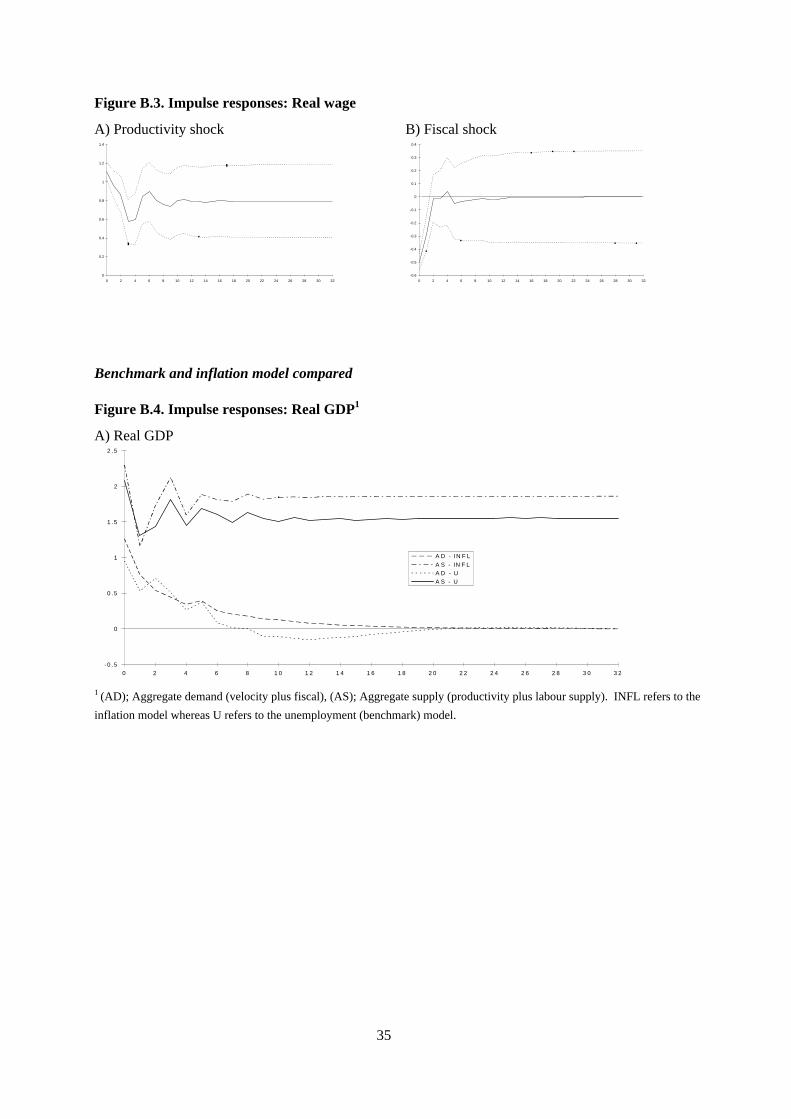
35

Figure B.3. Impulse responses: Real wage

A) Productivity shock B) Fiscal shock

0

0.2

0.4

0.6

0.8

1

1.2

1.4

0 2 4 6 8 10 12 14 16 18 20 22 24 26 28 30 32

-0.6

-0.5

-0.4

-0.3

-0.2

-0.1

0

0.1

0.2

0.3

0.4

0 2 4 6 8 10 12 14 16 18 20 22 24 26 28 30 32

Benchmark and inflation model compared

Figure B.4. Impulse responses: Real GDP1

A) Real GDP

-0 .5

0

0 .5

1

1 .5

2

2 .5

0 2 4 6 8 1 0 1 2 1 4 1 6 1 8 2 0 2 2 2 4 2 6 2 8 3 0 3 2

A D - IN F L

A S - IN F LA D - UA S - U

1 (AD); Aggregate demand (velocity plus fiscal), (AS); Aggregate supply (productivity plus labour supply). INFL refers to the

inflation model whereas U refers to the unemployment (benchmark) model.

36

Table B.1. Variance Decompositions of GDP and price1

GDP PriceQuarters PR LS VEL FI PR LS VEL FI1 18.4 58.5 17.4 5.7 2.8 69.2 27.1 0.94 27.2 56.5 9.4 6.9 1.1 50.9 40.5 7.512 24.0 68.9 4.0 3.2 3.4 43.6 36.6 16.432 19.8 77.6 1.5 1.2 4.4 40.8 35.2 19.51 (PR); Productivity shock, (LS); Labour supply shock, (VEL); Velocity shock and (FI); Fiscal shock.

Table B.2. Variance Decompositions of real exchange rate and real wage1

Real exchange rate Real wageQuarters PR LS VEL FI PR LS VEL FI1 18.1 5.1 7.6 69.2 82.1 1.3 0.3 16.44 19.9 3.2 9.8 67.0 88.1 1.5 1.6 8.912 22.6 5.7 3.7 68.0 94.4 0.8 0.9 3.932 22.6 8.1 1.1 68.1 97.7 0.3 0.4 1.61 See footnote 1 table B.1 for definitions.

37

Appendix C. Sample estimation

The benchmark model

Figure C.1. Impulse responses, full sample (1973-1994) and short sample (1973-1987) compared: 1

A) GDP B) GDP

-0.2

0

0.2

0.4

0.6

0.8

1

1.2

1.4

1.6

0 2 4 6 8 10 12 14 16 18 20 22 24 26 28 30 32

LSLS 73-87VELVEL 73-87

0

0.2

0.4

0.6

0.8

1

1.2

0 2 4 6 8 10 12 14 16 18 20 22 24 26 28 30 32

PRPR 73-87

C) Real exchange rate D) Real exchange rate

-1.6

-1.4

-1.2

-1

-0.8

-0.6

-0.4

-0.2

0

0.2

0.4

0 2 4 6 8 10 12 14 16 18 20 22 24 26 28 30 32

LSLS 73-87FIFI 73-87VELVEL 73-87

-1.6

-1.4

-1.2

-1

-0.8

-0.6

-0.4

-0.2

0

0 2 4 6 8 10 12 14 16 18 20 22 24 26 28 30 32

PRPR 73-87

E) Unemployment F) Real wage

-0.2

-0.15

-0.1

-0.05

0

0.05

0.1

0.15

0 2 4 6 8 10 12 14 16 18 20 22 24 26 28 30 32

LSLS 73-87VELVEL 73-87

-0.6

-0.4

-0.2

0

0.2

0.4

0.6

0.8

1

1.2

0 2 4 6 8 10 12 14 16 18 20 22 24 26 28 30 32

PRPR 73-87FIFI 73-87

1(PR); Productivity shock, (LS); Labour supply shock, (VEL); Velocity shock and (FI); Fiscal shock. 73-87 refers to the impulse

responses using the short sample (1973-1987).

38

Table C.1. Variance decompositions of GDP, (1973-1987)1

Benchmark model Inflation modelQuarters PR LS VEL FI PR LS VEL FI1 5.1 50.4 32.8 11.8 9.6 51.9 32.0 6.64 8.1 54.5 29.2 8.2 15.9 53.9 20.4 9.812 8.2 68.9 17.3 5.7 14.6 71.8 9.0 4.832 10.6 78.0 8.6 2.8 12.3 82.5 3.4 1.91) (PR); Productivity shock, (LS); Labour supply shock, (VEL); Velocity shock and (FI); Fiscal shock.

Table C.2. Variance decompositions of real exchange rate, (1973-1987)1

Benchmark model Inflation modelQuarters PR LS VEL FI PR LS VEL FI1 23.5 14.3 0.1 62.2 27.0 0.5 9.9 62.64 32.8 7.7 1.0 59.2 34.9 0.5 11.2 53.612 36.3 7.4 1.0 56.0 33.6 2.7 3.7 60.032 37.9 7.3 0.1 54.7 31.0 4.7 1.2 63.21) See footnote 1, table C.1 for definitions

Table C.3. Variance decompositions of real wage, (1973-1987)1

Benchmark model Inflation modelQuarters PR LS VEL FI PR LS VEL FI1 75.3 4.1 1.1 19.6 77.8 0.4 2.7 19.14 83.2 2.7 1.4 12.8 84.6 1.6 2.0 11.912 92.0 1.3 0.7 6.1 92.5 0.9 1.2 5.332 96.6 0.5 0.3 2.5 96.8 0.4 0.5 2.21) See footnote 1, table C.1 for definitions

Table C.4. Variance decompositions of unemployment, (1973-1987)1

Benchmark modelQuarters PR LS VEL FI1 0.1 24.2 72.4 3.34 5.4 8.2 82.5 3.912 4.0 6.1 74.6 15.332 4.1 6.0 74.7 15.31) See footnote table C.1 for definitions

Table C.5. Variance decompositions of price, (1973-1987)1

Inflation modelQuarters PR LS VEL FI1 2.1 73.3 14.8 9.84 0.2 51.4 27.3 21.112 1.4 43.6 26.2 28.932 1.8 41.2 25.7 31.31 See footnote table C.1 for definitions

39

Appendix D. An open economy with oil price shocks

The open economy model presented in section two is here augmented to allow for oil price shocks.

(D.1) y m p d e p p ot t t t t t t= − + + + + − +αθ β φ( * )

(D.2) y n ot t t t= + +θ ρ

(D.3) p w ot t t t= − +θ ψ

(D.4) [ ]w w E n nt t t t= =− −1 1

(D.5) n w pt t t t= − +γ λ( )

(D.6) ( * )e p p m d ot t t t t t+ − = + + + +∆ π δθ σλ κ

where o is the log of the real oil price. Equation (D.1) states that aggregate demand will now also be afunction of the real oil price. φ>0 is plausible in an economy with a large energy producing sector, ashigher real oil prices may increase demand from energy producers (like the government). The productionfunction in (D.2) relates output to the real oil price as a third factor of production. The real oil price isused instead of an energy quantity, as competitive producers treat the real oil price as parametric (seealso Bjørnland, 1996). Hence, we would expect (ρ<0). The price setting behaviour in (D.3) gives the CPIas a mark up on the real oil price, (ψ>0). Finally, the real exchange rate also varies with the oil price.Especially, if the Norwegian currency is a petrocurrency it appreciates when the oil price is high anddepreciates when the oil price is low (κ<0).

Assume that the oil price evolves as a random walk, driven by orthogonal oil price shocks (εOP):

(D.7) o ot t tOP= +−1 ε

Solving for ∆y, u, ∆(w-p) and ∆(e+p*-p) then yields:

(D.8) ∆ ∆ ∆ ∆ ∆

∆ ∆

yt tVEL

tFI

tPR

tPR

tLS

tLS

tOP

tOP

tOP

tOP

= + + + + + + − + + + +

+ + − + +−

− −

( ) ( ) ( ) ( )

( ) [( ) ]

1 1 1

1

1

1 1

β ε βπ ε γ ε α γ βδ ε ε βσ ε

ρε φ βκ ε ψ βδγ ε γε

(D.9)ut t

VELtFI

tPR

tLS

tOP

tOP

= − + − + − − + + − + − − +

+ −

( ) ( ) ( ) ( ) ( )

( )

1 1 1

1

β ε βπ ε α γ βδ ε βσ ε ρ φ βκ ε

ψ βδγ γ ε

(D.10) ∆( )w p t tPR

tOP− = −ε ψε

40

(D.11) ∆ ∆( * ) ( )e p p t tVEL

tFI

tPR

tLS

tOP+ − = + + + + −ε πε δε σε κ ψδγ ε

From the set of equations above, one can conclude that an oil price shock can have a long run effect onall the variables except the unemployment rate. The short term effects are more complicated to establish,and depend on which factors dominate. For instance, whereas an oil price shock (that increases the oilprice) will have a short term positive effect on GDP through increased aggregate demand (φ>0), theremay be negative short term effects on GDP if the Norwegian currency is a petro currency that appreciateswith a higher oil price (κ<0) and if the price level increases (ψ>0). however, in the long run, GDP fallswith a higher real oil price as the production function shifts down (ρ<0).

Ordering the vector of the five stationary variables as zt = (∆o, ∆rwt, ∆yt, ∆st, ut)' and the five seriallyuncorrelated orthogonal structural shocks as: εt = (εt

OP, εt PR, εt

LS, εt FI, εt

VEL )', the long run expressionof the moving average expression of zt, can then be written as:

(D.12)

∆∆∆∆

o

rw

y

s

u

D D D D D

D D D D D

D D D D D

D D D D D

D D D D Dt

OP

PR

LS

FI

VEL

=

11 12 13 14 15

21 22 23 24 25

31 32 33 34 35

41 42 43 44 45

51 52 53 54 55

1 1 1 1 1

1 1 1 1 1

1 1 1 1 1

1 1 1 1 1

1 1 1 1 1

( ) ( ) ( ) ( ) ( )

( ) ( ) ( ) ( ) ( )

( ) ( ) ( ) ( ) ( )

( ) ( ) ( ) ( ) ( )

( ) ( ) ( ) ( ) ( )

ε

εε

εε

t

The model presented above implies that only oil price shock can have a long run effect on oil prices: 17

(D.13) D12(1)=D13(1)=D14(1)=D15(1) = 0.

Productivity shocks and oil price shocks can affect real wages in the long run:

(D.14) D23(1) = D24(1) = D25(1) = 0.

All three productivity, labour supply and oil price shocks can affect output in the long run:

(D.15) D34(1) = D35(1) = 0

and all shocks but velocity can affect the real exchange rate in the long run:

(D.16) D45(1) = 0

With these ten long run restrictions, it is now easy to see that the matrix D(1) will be lower triangular,and we can use this to recover D0.

17 In Bjørnland (1996), I allowed demand and supply shocks to affect the real price of oil in the long run. However, byexamination, none of these shocks turned out to have significant long run effects on real oil prices in Norway.

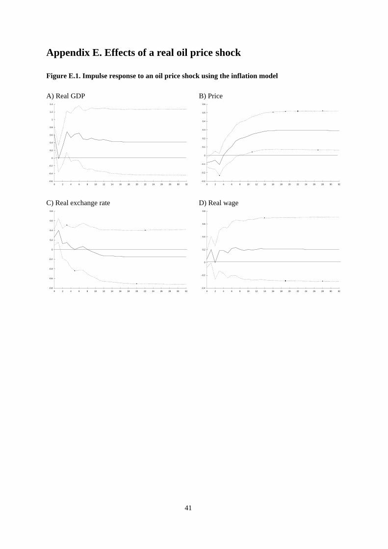
41

Appendix E. Effects of a real oil price shock

Figure E.1. Impulse response to an oil price shock using the inflation model

A) Real GDP B) Price

-0.6

-0.4

-0.2

0

0.2

0.4

0.6

0.8

1

1.2

1.4

0 2 4 6 8 10 12 14 16 18 20 22 24 26 28 30 32-0.3

-0.2

-0.1

0

0.1

0.2

0.3

0.4

0.5

0.6

0 2 4 6 8 10 12 14 16 18 20 22 24 26 28 30 32

C) Real exchange rate D) Real wage

-0.8

-0.6

-0.4

-0.2

0

0.2

0.4

0.6

0.8

0 2 4 6 8 10 12 14 16 18 20 22 24 26 28 30 32-0.4

-0.2

0

0.2

0.4

0.6

0.8

0 2 4 6 8 10 12 14 16 18 20 22 24 26 28 30 32

42

Table E.1. Variance decompositions of GDP and unemployment using the benchmark model

GDP UnemploymentQuarters OP PR LS VEL FI OP PR LS VEL FI1 4.2 17.0 39.8 38.4 1.0 4.8 1.9 33.6 48.6 11.14 5.4 22.1 40.8 31.2 0.5 4.5 5.9 16.3 60.2 13.212 12.6 18.1 53.0 15.5 0.8 3.2 5.2 11.1 68.1 12.520 14.3 16.3 60.0 9.9 0.5 3.2 5.3 10.9 68.1 12.71) OP; Oil price shock, PR; Productivity shock, LS; Labour supply shock, VEL; Velocity shock and FI; Fiscal shock.

Table E.2. Variance decompositions of real exchange rate and real wage using the benchmarkmodel

Real exchange rate Real wageQuarters OP PR LS VEL FI OP PR LS VEL FI1 3.6 12.4 11.7 5.3 67.1 0.0 88.6 1.5 0.0 9.94 3.2 14.3 9.1 4.2 69.2 1.7 91.2 1.5 0.2 5.412 1.0 18.9 8.9 1.8 69.4 2.8 93.9 0.7 0.3 2.420 0.7 20.6 8.9 1.1 68.8 3.0 94.9 0.4 0.2 1.51) See footnote 1, table E.1 for definitions.

Table E.3. Variance decompositions of price using the inflation model

Quarters OP PR LS VEL FI1 3.5 1.4 66.8 27.4 0.94 1.4 0.3 52.5 38.1 7.812 2.0 0.5 43.4 34.7 19.620 3.3 0.6 40.0 34.8 21.41 See footnote 1, table E.1 for definitions.