highly accurate attitude estimation via horizon detection
TRANSCRIPT

Highly Accurate Attitude Estimation via Horizon
Detection Bertil Grelsson, Michael Felsberg and Folke Isaksson
The self-archived postprint version of this journal article is available at Linköping
University Institutional Repository (DiVA):
http://urn.kb.se/resolve?urn=urn:nbn:se:liu:diva-108212
N.B.: When citing this work, cite the original publication. Grelsson, B., Felsberg, M., Isaksson, F., (2016), Highly Accurate Attitude Estimation via Horizon Detection, Journal of Field Robotics, 33(7), 967-993. https://doi.org/10.1002/rob.21639
Original publication available at: https://doi.org/10.1002/rob.21639
Copyright: Wiley (12 months) http://eu.wiley.com/WileyCDA/
Highly accurate attitude estimation via horizon
detection
Bertil Grelsson∗
Saab DynamicsSaab, Linkoping, Sweden
Michael FelsbergComputer Vision LaboratoryLinkoping University, [email protected]
Folke IsakssonVricon Systems
Saab, Linkoping, [email protected]
Abstract
Attitude (pitch and roll angle) estimation from visual information is necessary for GPS freenavigation of airborne vehicles. We propose a highly accurate method to estimate the at-titude by horizon detection in fisheye images. A Canny edge detector and a probabilisticHough voting scheme are used to compute an approximate attitude and the correspondinghorizon line in the image. Horizon edge pixels are extracted in a band close to the approxi-mate horizon line. The attitude estimates are refined through registration of the extractededge pixels with the geometrical horizon from a digital elevation map (DEM), in our casethe SRTM3 database. The proposed method has been evaluated using 1629 images from aflight trial with flight altitudes up to 600 m in an area with ground elevations ranging fromsea level up to 500 m. Compared with the ground truth from a filtered IMU/GPS solution,the standard deviation for the pitch and roll angle errors are 0.04◦ and 0.05◦, respectively,with mean errors smaller than 0.02◦. To achieve the high accuracy attitude estimates, theray refraction in the earth atmosphere has been taken into account. The attitude errorsobtained on real images are less or equal to those achieved on synthetic images for previousmethods with DEM refinement, and the errors are about one order of magnitude smallerthan for any previous vision-based method without DEM refinement.
1 Introduction
For autonomous navigation of unmanned aerial vehicles (UAVs), online estimation of the absolute positionand attitude of the vehicle is required. For attitude estimation, inertial measurement units (IMUs) arecommonly used but they suffer from drift and need support to give reliable estimates over time. Pilotsin manned aircraft intuitively use the horizon as an attitude reference. Using the same basic concept,many vision-based methods have been presented where horizon detection is employed for absolute attitudeestimates. Most of these methods include either an explicit or implicit assumption that the horizon line issmooth, (Natraj et al., 2013), (Mondragon et al., 2010), (Moore et al., 2011b), (Grelsson and Felsberg, 2013),(Bao et al., 2003), (Dusha et al., 2011) and (Dumble and Gibbens, 2012). In this context, we define the
∗Alternative address: Computer Vision Laboratory, Linkoping University, Sweden. E-mail [email protected]

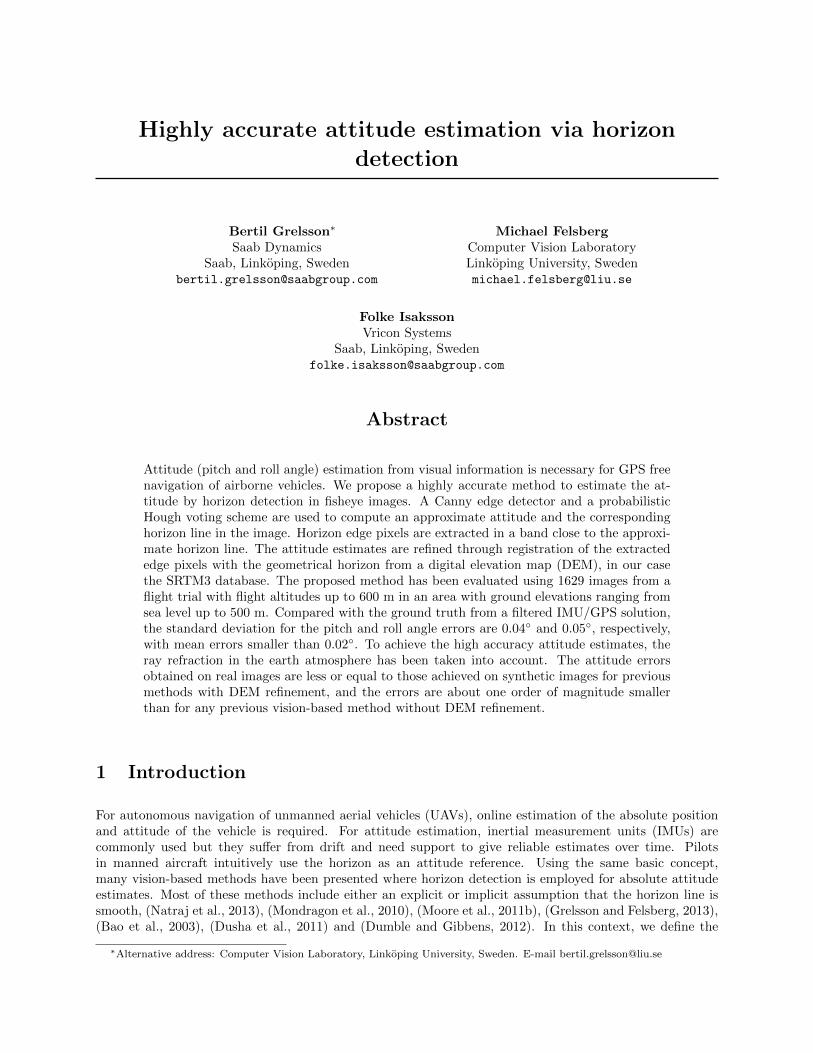
(a) (b) (c)
Figure 1: (a) Definition of vehicle pose, ψ = yaw, θ = pitch, φ = roll. (b), (c) Aerial fisheye images withestimated horizon overlaid.
horizon as the boundary line between the sky and the ground/sea pixels in the image. The cited methodsoften search for or approximate the horizon as straight lines in perspective images or perfect ellipses inomnidirectional images. The attitude accuracy obtained with these methods is often around 1-2◦. Thisaccuracy is sufficient if your aim is to control and stabilize a UAV during flight, even for rather extrememaneuvers (Thurrowgood et al., 2010). But for autonomous surveillance and reconnaissance missions withflight durations around an hour covering distances in the order of 100 km, this attitude accuracy is farfrom adequate. The position estimates would drift away and hence the UAV would deviate too far from itsintended route implying that the estimated position for localized objects of interest in the images would bevery inaccurate. A constant 1◦ attitude error for a 100 km flight results in a position error around 2 km.For these types of missions absolute attitude accuracies better than 0.1◦ are often required throughout theflight.
In a recent paper (Dumble and Gibbens, 2014), a method is proposed where the measured 360◦ horizonprofile from a set of aerial perspective images is aligned with a reference horizon profile computed from adigital elevation model (DEM) to estimate the attitude and the position of the platform. This is the onlymethod we have encountered that can provide these high accuracy attitude estimates However, as will bediscussed later, this method requires a large horizon profile variance and that the distance to the perceivedhorizon is relatively short (<40 km). This makes the method ideal for, but also restricted to, mountainousterrain like the Alps, where the method was evaluated.
Mountainous terrain, with ground elevations greater than 2 km, accounts for about 4% of the total areaon earth (Encyclopaedia Britannica, 2014). Terrain with ground elevations lower than one kilometer is byfar the most common land type on earth covering more than 20% of the total area and around 70% ofthe total land area on earth. Moreover, urban areas account for only 3% of the total land area on earth(NewGeography, 2010). Attitude estimation methods for low altitude flights in urban environment have beenadressed in e.g. (Bazin et al., 2008) and (Demonceaux et al., 2007). Our aim is to develop a method thatprovides highly accurate attitude estimates in the most common terrain type, i.e. flying above tree tops andbuildings in terrain with ground elevations up to a kilometer.
We present a novel method for highly accurate estimation of the pitch and roll angles of an airborne vehiclevia horizon detection in fisheye images, see figure 1(a) for definitions of angles. We use 30 MPixel imageswith a frame rate of around 1 fps. The attitude estimates are refined through registration of the perceivedhorizon with the geometrical horizon from a DEM. To the best of our knowledge, this is the first proposedmethod for aerial omnidirectional images where the detected horizon is refined with DEM data for attitudeestimation. The method has been evaluated using 1629 aerial images from an 80 km long flight at up to600 m altitude in an area with woodlands, cities, lakes and the sea. Example images with the estimatedhorizon overlaid are shown in figure 1(b) and (c). The ground elevation in the flight area affecting the horizonranges from sea level up to about 500 m altitude. Our vision-based method is primarily intended to supportnavigation for small UAVs that cannot carry highly accurate IMUs due to both cost and payload weightrestrictions.
The key components of the proposed method to achieve the high accuracy are:
1. The use of fisheye (omnidirectional) images, where a large portion of the horizon can be seen irre-spectively of the vehicle orientation.
2. Accurate calibration of the fisheye lens, especially close to the fisheye border.
3. Accurate detection and extraction of the horizon line in the fisheye image.
4. Registration of the perceived horizon line in the image with the geometrical horizon from a DEM.
5. Taking into account the refraction of oblique rays in the earth atmosphere.
The use of these components in a horizon detection method for attitude estimation is motivated as follows.For an airborne vehicle, the use of omnidirectional images is appropriate to ensure that the horizon will beseen in the image even for large attitude angles. Furthermore, omnidirectional images contain informationon a larger fraction of the complete horizon line compared to perspective images and this makes the methodmore robust to partial occlusion of the horizon. The requirement for accurate camera calibration is obviousbut is hard to obtain close to the fisheye circle, i.e. almost perpendicular to the optical axis. For highaccuracy attitude estimates, registration with a DEM is necessary unless the terrain is truly flat and levelwhich is rarely the case. If a DEM is used, the true horizon profile must be extracted from the image forhigh accuracy attitude estimates. In our test flight, the true horizon was often offset 4-5 pixels from the idealhorizon ellipse on the image plane. Approximations with a straight line (perspective image) or a perfectellipse (omnidirectional image) assuming a level terrain will generate attitude errors depending on the trueground topography.
Finally, refraction correction results in a further improvement of accuracy. For airborne vehicles at 500-1000 m altitude, the true incidence angle for refracted rays from the sea level horizon will be around 0.05◦-0.1◦ greater than if assuming straight ray propagation. This deviation would generate errors and shows thatfor high accuracy attitude estimates, the refraction in the atmosphere needs to be taken into account.
The main contribution of this paper is a method to detect and extract the true horizon line in fisheye images.This is achieved by first estimating an approximate horizon line by edge detection and a probabilistic Houghvoting scheme (Grelsson and Felsberg, 2013) assuming that the earth is an ideal sphere. The true horizonline in the image is then extracted from edge pixels in a thin band ranging from the approximate, idealhorizon to an outer limit in the image plane, depending on the ground elevation taken from the DEM.
A second contribution is the proposed method of using the extracted horizon line and the geometricallyexpected horizon for accurate calibration of the fisheye lens. This calibration method requires accurateknowledge of the 6DOF camera position when the images were captured. The proposed calibration methodwas employed to refine the camera calibration in our test flight.
A third contribution is taking the ray refraction in the atmosphere into account when computing the ge-ometric horizon line from DEM data. If ray refraction is ignored, a systematic attitude estimate offset isintroduced which is a significant error source for high accuracy attitude estimate methods.
This paper is organized as follows. Section 2 gives a review of image based methods for vehicle attitude esti-mation, focusing on methods using horizon detection, DEMs, or omnidirectional images. Section 3 presentsthe camera and earth models used. An overview of the attitude estimation method and its prerequisites isgiven in section 4. A detailed description of the proposed method is presented in section 5. In section 6,the flight trial performed for evaluation of the proposed method is described. Section 7 presents the resultsobtained with the attitude estimation method. It also provides an analysis to explain the results and themain error sources. Finally, the conclusions are given in section 8.
2 Related work
Vision-based methods are frequently applied for attitude estimation of a vehicle. Our proposed methodis designed for attitude estimation of an airborne vehicle and employ horizon detection in omnidirectionalimages with DEM based refinement. To the best of our knowledge no method exist that use all thesecomponents for attitude estimation and we focus on related methods which are based on horizon detectionand contain at least one of the other components. The components employed in the related methods andthe accuracy of the attiude estimates obtained are summarized in table 1.
Table 1: Related methods and results.First author Vehicle Camera DEM Accuracy pitch/roll Comments
Natraj Airborne Omnidir. No Mean error 2.5-3.0◦
Bazin Airborne Omnidir. No Not applicableMondragon Airborne Omnidir. No RMSE 0.2-4.4◦ Yaw angle estimatedThurrowgood Airborne Omnidir. No Average error 1-2◦ Manual horizon as ground truthMoore 2011a Airborne Omnidir. No Average error 1.5◦ Manual horizon as ground truthMoore 2011b Airborne Omnidir. No Average error 1.5◦ Yaw angle estimatedGrelsson Airborne Omnidir. No Not reported No attitude ground truth availableBao Airborne Perspective No Not reported No attitude ground truth availableDusha Airborne Perspective No σ = 1.8◦ (flight 1) Pose estimates filtered with EKF
σ = 0.4-0.7◦ (flight 2)Dumble 2012 Airborne Perspective No σ = 0.9-1.0◦
Dumble 2014 Airborne Perspective Yes σ = 0.07◦ and 0.03◦ Location estimated, synthetic imagesGupta Ground Perspective Yes 2σ = 0.50◦ and 0.26◦ IMU supported, yaw angle estimated
An overview of available methods where horizon detection is used to infer the camera attitude for airbornevehicles is given in (Shabayek et al., 2012). Work on horizon detection in omnidirectional images is ratherlimited. In (Natraj et al., 2013) horizon detection is used for attitude estimation in catadioptric images froma rural area. A sky/ground segmentation is performed based on pixel color content using Markov RandomFields. The detected horizon line is projected onto the unit sphere and a best fit to a plane on the sphere iscomputed, assuming a smooth horizon line and implicitly a level terrain. A method to extract the skyline incatadioptric IR images is proposed in (Bazin et al., 2009). It is also suggested in the paper that the extractedskyline could be registered with the skyline from a DEM for attitude estimation, but no registration methodis proposed. The skyline is extracted in synthetic IR-like images since the catadioptric mirrors required forimage formation are not commercially available.
For catadioptric images, a sky/ground segmentation method based on the pixel RGB color content in apyramid segmentation is used in (Mondragon et al., 2010). Horizon pixels are projected onto the unit sphereto estimate the best fit of a plane which is then used to estimate the pitch and roll angles. The relativeheading angle between images is estimated by searching for a best match using an image column shift,implicitly assuming a pure rotation around the vertical axis.
Spectral and intensity properties are used to classify sky and ground regions in the image in (Thurrowgoodet al., 2010). The classification rule is precomputed and based on a training set of images. Horizon edges arefitted to a 3D plane on the viewsphere to infer the attitude angles. The same group of authors presents anonline learning method to classify the image into sky/ground based on spectral information and brightness(Moore et al., 2011a). The aircraft attitude is obtained by exhaustively matching the classified input imageagainst a database of ideal image classifications, representing all possible attitude combinations. The sameauthors add a visual compass to also estimate the heading angle in (Moore et al., 2011b). Stabilizedpanoramic views, compensated for the estimated pitch and rolled angles, are compared with a reference viewto infer the change in heading direction.
For horizon detection and attitude estimation from aerial fisheye images, (Grelsson and Felsberg, 2013) useedge detection and a probabilistic Hough voting scheme. The method presented is used as a basis for the
proposed attitude estimation method in this paper.
For perspective images there are two main approaches for horizon detection, either edge detection orsky/ground segmentation using pixel color characteristics. A common technique for edge based methodsis presented in (Bao et al., 2003) where edge pixels vote for horizon line directions and positions in a Houghvoting scheme to infer the camera pitch and roll angles. In (Dusha et al., 2011) a state vector consisting ofthe pitch and roll angles and the aircraft body rates are estimated from horizon detection and optical flowin images from a perspective, front-mounted camera. Edge detection and Hough voting is used to generatecandidate horizon lines, and optical flow is used to reject lines that are not close to the true horizon.
In a recent work (Dumble and Gibbens, 2012) a search for horizon pixels is performed in each column basedon gradient thresholding and pixel color content. They look for a contiguous line of horizon pixels extendingacross the whole image but do not require the line to be straight. A gradient threshold is varied until onlyone line across the image remains, which is taken as the horizon. The best fit of the contiguous line to astraight line is made, implying that valuable horizon profile information will not be used in the subsequentattitude estimation.
The same authors extend their work (Dumble and Gibbens, 2014) and now include alignment of the measuredhorizon profile with a reference horizon profile from a DEM to estimate the attitude as well as the locationof the airborne platform. A set of four perspective cameras is used to obtain a complete 360◦ view of thehorizon. To speed up the method considerably, the horizon profile is pre-computed from DEM data at a setof 3D grid points. The horizon profile is extracted from the closest grid point to the assumed 3D position.Using a horizon profile transformation scheme, the reference horizon profile is transformed to the currentlyassumed 6DoF position. To refine the estimated location and attitude of the platform, the total pitch angledifference between the measured horizon and the transformed reference horizon is iteratively minimized. Toevaluate the method, synthetic images from a flight simulator program is used. Images are rendered froma virtual flight along a valley in the Alps where the horizon profile variance is very large. Presumably (notmentioned in the paper), the same flight simulator is used as a DEM to generate the reference horizon profiles.The results obtained are very impressive. The attitude errors are at least one order of magnitude smallerthan for any previous method without DEM refinement. Since this method (Dumble and Gibbens, 2014)is the one most similar to ours, we will return to it in section 7.5 and present a more detailed comparisonbetween this method and ours together with an analysis of the results obtained with the two methods.
There are several other methods proposed for attitude estimation using horizon silhouette matching inmountainous areas (Naval Jr. et al., 1997), (Behringer, 1998), (Woo et al., 2007), (Baatz et al., 2012). Thesemethods often rely on detection of mountain peaks and we are looking for a more general method for horizonregistration.
Gupta and Brennan present one approach for registering the true horizon line in an image with DEM datafor refined attitude estimation for a ground vehicle (Gupta and Brennan, 2008). Information from a front-mounted perspective camera and an IMU is fused and registered with DEM data to estimate the absoluteyaw, pitch and roll angles. The attitude accuracy obtained is better than for any method without DEMrefinement but the accuracy is somewhat inferior to recent results (Dumble and Gibbens, 2014). The mainreasons for this are probably the smaller FOV and a smaller horizon profile variance in the images.
We are not aware of any previous method for attitude estimation taking the ray refraction in the earthatmosphere into account. Equations for refracted ray propagation are given in (Gyer, 1996). The effect issmall and the attitude errors induced are often smaller than the errors from the assumption that the horizonis generated by a level terrain. However, for high accuracy attitude measurements using the horizon fromairborne vehicles, the ray refraction effect cannot be neglected. For aircraft flying at 500 m altitude, attitudeerrors in the order of 0.05◦ are introduced if neglecting ray refraction to the ideal horizon at sea level.
3 Camera and earth models
3.1 Camera model
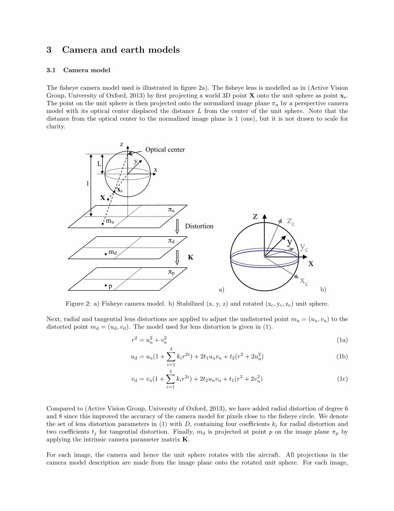
The fisheye camera model used is illustrated in figure 2a). The fisheye lens is modelled as in (Active VisionGroup, University of Oxford, 2013) by first projecting a world 3D point X onto the unit sphere as point xs.The point on the unit sphere is then projected onto the normalized image plane πu by a perspective cameramodel with its optical center displaced the distance L from the center of the unit sphere. Note that thedistance from the optical center to the normalized image plane is 1 (one), but it is not drawn to scale forclarity.
1
L x
z
y
X x s
mu
π u
π d
π p
md
Distortion
p
K
Optical center
a)
x
z
y
zc
yc
xc b)
Figure 2: a) Fisheye camera model. b) Stabilized (x, y, z) and rotated (xc, yc, zc) unit sphere.
Next, radial and tangential lens distortions are applied to adjust the undistorted point mu = (uu, vu) to thedistorted point md = (ud, vd). The model used for lens distortion is given in (1).
r2 = u2u + v2u (1a)
ud = uu(1 +
4∑i=1
kir2i) + 2t1uuvu + t2(r2 + 2u2u) (1b)
vd = vu(1 +
4∑i=1
kir2i) + 2t2uuvu + t1(r2 + 2v2u) (1c)
Compared to (Active Vision Group, University of Oxford, 2013), we have added radial distortion of degree 6and 8 since this improved the accuracy of the camera model for pixels close to the fisheye circle. We denotethe set of lens distortion parameters in (1) with D, containing four coefficients ki for radial distortion andtwo coefficients tj for tangential distortion. Finally, md is projected at point p on the image plane πp byapplying the intrinsic camera parameter matrix K.
For each image, the camera and hence the unit sphere rotates with the aircraft. All projections in thecamera model description are made from the image plane onto the rotated unit sphere. For each image,
we also consider a north-aligned and vertically stabilized unit sphere with the same center position as therotated unit sphere. The ideal horizon from the sea level will generate a horizontal circle on the stabilizedunit sphere, see figure 2b). The geometrical horizon from the DEM will be computed on the stabilized unitsphere. The camera rotation matrix bwRc denotes the rotation from the stabilized unit sphere to the rotatedunit sphere, i.e. it transforms a point wP in the stabilized world frame to its coordinates bP in the camerabody frame such that
bP = bwRcwP. (2)
3.2 Earth model and refracted ray propagation
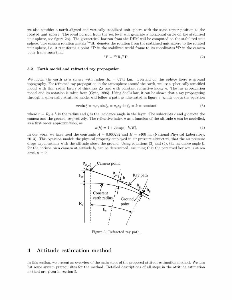
We model the earth as a sphere with radius Re = 6371 km. Overlaid on this sphere there is groundtopography. For refracted ray propagation in the atmosphere around the earth, we use a spherically stratifiedmodel with thin radial layers of thickness ∆r and with constant refractive index n. The ray propagationmodel and its notation is taken from (Gyer, 1996). Using Snells law, it can be shown that a ray propagatingthrough a spherically stratified model will follow a path as illustrated in figure 3, which obeys the equation
nr sin ξ = ncrc sin ξc = ngrg sin ξg = k = constant (3)
where r = Re + h is the radius and ξ is the incidence angle in the layer. The subscripts c and g denote thecamera and the ground, respectively. The refractive index n as a function of the altitude h can be modelled,as a first order approximation, as
n(h) = 1 +A exp(−h/B). (4)
In our work, we have used the constants A = 0.000292 and B = 8400 m, (National Physical Laboratory,2013). This equation models the physical property employed in air pressure altimeters, that the air pressuredrops exponentially with the altitude above the ground. Using equations (3) and (4), the incidence angle ξcfor the horizon on a camera at altitude hc can be determined, assuming that the perceived horizon is at sealevel, h = 0.
R e
h c h
h g ξ g
ξ c
ξ
Camera point
Ground point
Ray path
Constant earth radius
θ c
Figure 3: Refracted ray path.
4 Attitude estimation method
In this section, we present an overview of the main steps of the proposed attitude estimation method. We alsolist some system prerequisites for the method. Detailed descriptions of all steps in the attitude estimationmethod are given in section 5.
4.1 Algorithmic steps, overview
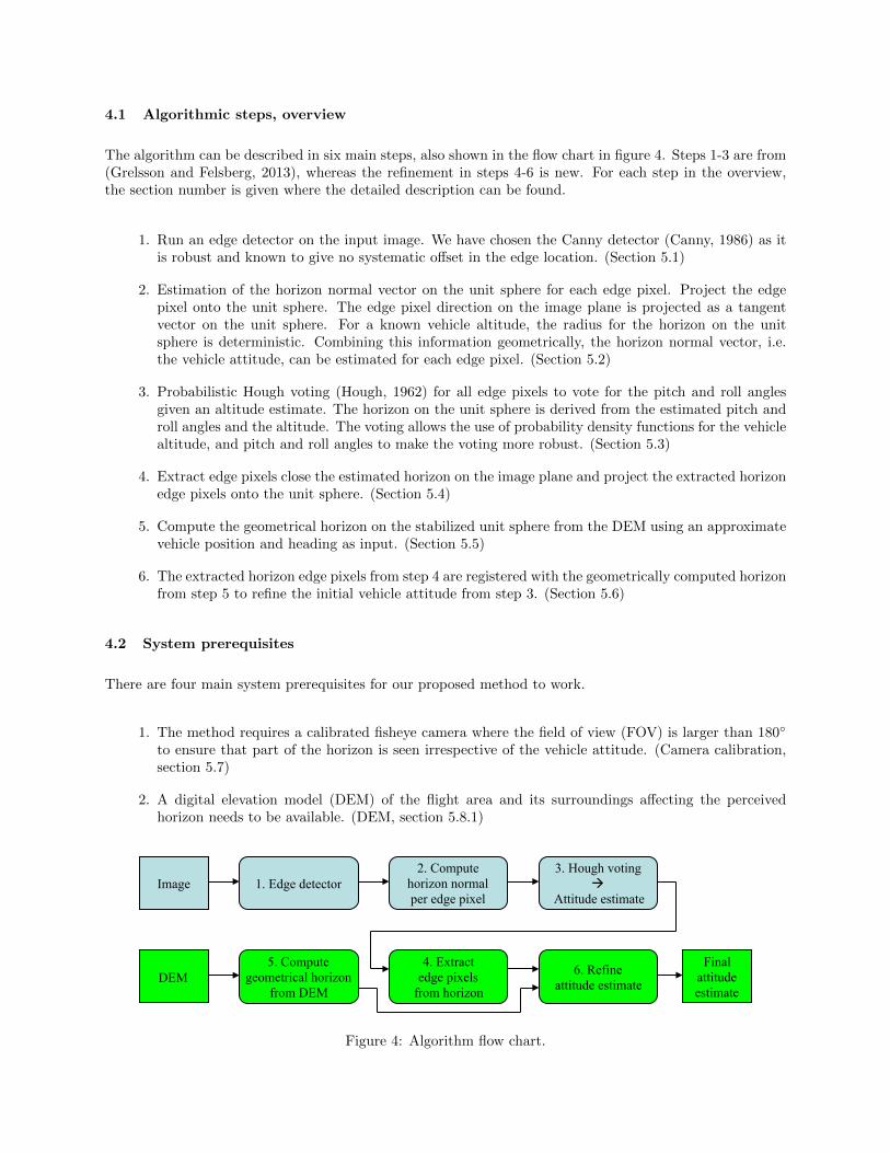
The algorithm can be described in six main steps, also shown in the flow chart in figure 4. Steps 1-3 are from(Grelsson and Felsberg, 2013), whereas the refinement in steps 4-6 is new. For each step in the overview,the section number is given where the detailed description can be found.
1. Run an edge detector on the input image. We have chosen the Canny detector (Canny, 1986) as itis robust and known to give no systematic offset in the edge location. (Section 5.1)
2. Estimation of the horizon normal vector on the unit sphere for each edge pixel. Project the edgepixel onto the unit sphere. The edge pixel direction on the image plane is projected as a tangentvector on the unit sphere. For a known vehicle altitude, the radius for the horizon on the unitsphere is deterministic. Combining this information geometrically, the horizon normal vector, i.e.the vehicle attitude, can be estimated for each edge pixel. (Section 5.2)
3. Probabilistic Hough voting (Hough, 1962) for all edge pixels to vote for the pitch and roll anglesgiven an altitude estimate. The horizon on the unit sphere is derived from the estimated pitch androll angles and the altitude. The voting allows the use of probability density functions for the vehiclealtitude, and pitch and roll angles to make the voting more robust. (Section 5.3)
4. Extract edge pixels close the estimated horizon on the image plane and project the extracted horizonedge pixels onto the unit sphere. (Section 5.4)
5. Compute the geometrical horizon on the stabilized unit sphere from the DEM using an approximatevehicle position and heading as input. (Section 5.5)
6. The extracted horizon edge pixels from step 4 are registered with the geometrically computed horizonfrom step 5 to refine the initial vehicle attitude from step 3. (Section 5.6)
4.2 System prerequisites
There are four main system prerequisites for our proposed method to work.
1. The method requires a calibrated fisheye camera where the field of view (FOV) is larger than 180◦
to ensure that part of the horizon is seen irrespective of the vehicle attitude. (Camera calibration,section 5.7)
2. A digital elevation model (DEM) of the flight area and its surroundings affecting the perceivedhorizon needs to be available. (DEM, section 5.8.1)
Image 1. Edge detector 2. Compute
horizon normal per edge pixel
3. Hough voting à
Attitude estimate
5. Compute geometrical horizon
from DEM
6. Refine attitude estimate
4. Extract edge pixels
from horizon DEM
Final attitude estimate
Figure 4: Algorithm flow chart.

3. A function is required that computes the ray path in the earth atmosphere from an object at altitudehobj to a camera at altitude hc where the object and the camera are separated a distance d. To obtainan attitude estimation method with real-time capability, we have implemented this functionality aslook-up tables as described in section 5.8.2.
4. An approximate vehicle position and heading is required to generate a geometric horizon from theDEM.
5 Detailed algorithm description
The first three subsections in the algorithm description, sections 5.1 - 5.3, are from (Grelsson and Felsberg,2013), the remainder of the algorithm is new.
5.1 Edge detector
The first step in our method is an edge detection and we use the Canny detector (Canny, 1986) as it is knownto give robust results with no systematic offset in the edge position. Before applying the Canny detector,the color image is converted to grayscale and the image is smoothed with a gaussian 3x3 kernel.
To reduce subsequent unnecessary computations in the Hough voting, we first remove some edge pixels thatwe know will not contribute to the horizon detection. In the edge image, there will be unwanted edge pixelsdue to the fisheye circle and the aircraft structure. These edge pixels will remain almost stationary on theimage plane throughout a flight.
To determine a background edge map, we collected 100 edge images from a flight. Each pixel that wasclassified as an edge pixel in more than 30% of the images was considered to be a background edge pixel,i.e. originating either from the fisheye circle or from the aircraft structure. This background edge map issubtracted from the Canny edge map for each image prior to the Hough voting. The 30% threshold was setempirically and its exact value is not crucial for the attitude estimate results.
5.2 Estimate horizon normal
For an image edge pixel p = (x,y), the projection onto the unit sphere is at point P . We compute thegradient in p with 3x3 sobel filters, and define the edge direction in p as (−∇y,∇x), i.e. normal to thegradient. We define the image point pe as the point one pixel away from p along the edge direction. The
projection of pe onto the unit sphere is at Pe. If p is a horizon point, the vector−−→PPe is a tangent vector on
the unit sphere lying in the plane of the projected horizon. Let t be a vector of unit length in the direction
of−−→PPe. If we look at a cross section of the unit sphere, orthogonal to the vector t, as in figure 5, we search
for a second point Q in the plane of the horizon. For a certain altitude h, the radius of the horizon circle onthe unit sphere is known. To find Q, we define the vector
−→OS =
−−→OP × t (5)
where O is the origin in the unit sphere. We then obtain the vector
−−→OQ =
−−→OP cos 2ξc +
−→OS sin 2ξc, (6)
where ξc is the incidence angle from the horizon for a camera at altitude hc. At this stage, we assume that theearth is smooth with radius Re. The points Qmax and Qmin denote the horizon points for the maximum andminimum altitudes given the probability distribution ph for the camera altitude in the subsequent voting.
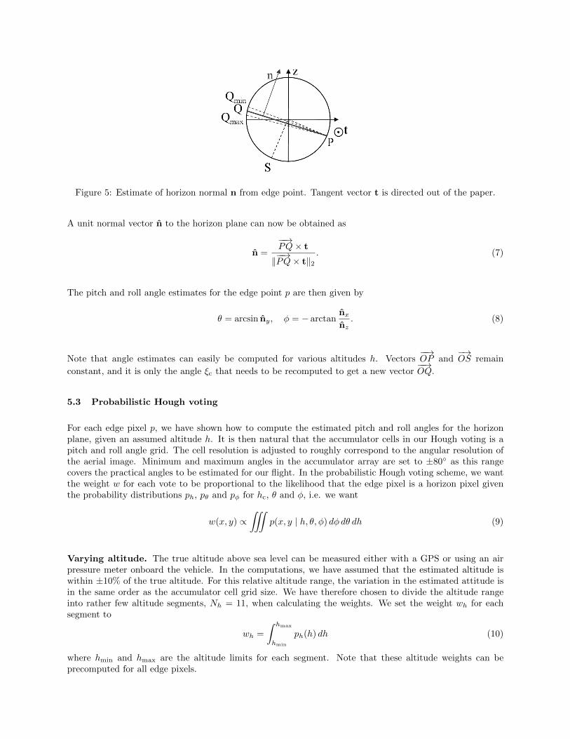
Figure 5: Estimate of horizon normal n from edge point. Tangent vector t is directed out of the paper.
A unit normal vector n to the horizon plane can now be obtained as
n =
−−→PQ× t
‖−−→PQ× t‖2
. (7)
The pitch and roll angle estimates for the edge point p are then given by
θ = arcsin ny, φ = − arctannxnz. (8)
Note that angle estimates can easily be computed for various altitudes h. Vectors−−→OP and
−→OS remain
constant, and it is only the angle ξc that needs to be recomputed to get a new vector−−→OQ.
5.3 Probabilistic Hough voting
For each edge pixel p, we have shown how to compute the estimated pitch and roll angles for the horizonplane, given an assumed altitude h. It is then natural that the accumulator cells in our Hough voting is apitch and roll angle grid. The cell resolution is adjusted to roughly correspond to the angular resolution ofthe aerial image. Minimum and maximum angles in the accumulator array are set to ±80◦ as this rangecovers the practical angles to be estimated for our flight. In the probabilistic Hough voting scheme, we wantthe weight w for each vote to be proportional to the likelihood that the edge pixel is a horizon pixel giventhe probability distributions ph, pθ and pφ for hc, θ and φ, i.e. we want
w(x, y) ∝∫∫∫
p(x, y | h, θ, φ) dφ dθ dh (9)
Varying altitude. The true altitude above sea level can be measured either with a GPS or using an airpressure meter onboard the vehicle. In the computations, we have assumed that the estimated altitude iswithin ±10% of the true altitude. For this relative altitude range, the variation in the estimated attitude isin the same order as the accumulator cell grid size. We have therefore chosen to divide the altitude rangeinto rather few altitude segments, Nh = 11, when calculating the weights. We set the weight wh for eachsegment to
wh =
∫ hmax
hmin
ph(h) dh (10)
where hmin and hmax are the altitude limits for each segment. Note that these altitude weights can beprecomputed for all edge pixels.
Voting. Using Bayes’ theorem and assuming that the probability distributions for hc, θ and φ are indepen-dent, we calculate the weights as
w(x, y) ∝∫ph(h) dh
∫pθ(θ) dθ
∫pφ(φ) dφ = whwθwφ (11)
For each edge pixel p, we compute the estimated pitch and roll angles for each altitude h and give a weightedvote in the nearest neighbor pitch-roll cell in the accumulator array. In our flight we had no prior informationon the pitch and roll angles and the weights wθ and wφ were set to 1. If you have prior information onthe attitude angles, e.g. from an onboard IMU giving the relative rotation from the last absolute attitudeestimate, the weights should be set in accordance with pθ and pφ over the pitch-roll grid.
Attitude estimate. In order to suppress local maxima, we convolve the values in the accumulator arraywith a gaussian kernel of size 7x7 and pick the index for the cell with maximum score as the attitude estimate.To refine the attitude estimate, we do a second order polynomial fit along the pitch and roll directions aroundthe accumulator array maximum. The result after this step is an attitude estimate where we have assumedan ideal smooth earth with radius Re. The results obtained in this way have been analyzed in (Grelsson andFelsberg, 2013).
5.4 Extract horizon edge pixels
Using the method from (Grelsson and Felsberg, 2013), we noticed significant attitude estimate errors dueto nonflat horizons and further refinement becomes necessary. To prepare for the refinement of the attitudeestimate, we want to extract only the edge pixels originating from the horizon in the image. We do thisgeometrically and extract edge pixels close to the estimated horizon from the Hough voting. For a perfectlycalibrated camera and exact knowledge of the camera altitude, the ellipse on the image plane correspondingto the estimated horizon from the Hough voting will always be slightly smaller than the true perceivedhorizon on the image due to the topography on top of the ideal spherical earth. Thus, most of the truehorizon edge pixels will be on or outside the estimated horizon. Due to quantization effects in the edgedetector (only integer pixels), some true horizon edge pixels may be 1/2 pixel inside the estimated horizon.If the shift of the horizon due to topography is less than 1 pixel, it is sufficient to project the estimatedhorizon on the image plane and extract all edge pixels that are within a 3x3 matrix from the horizon pixelson the image plane.
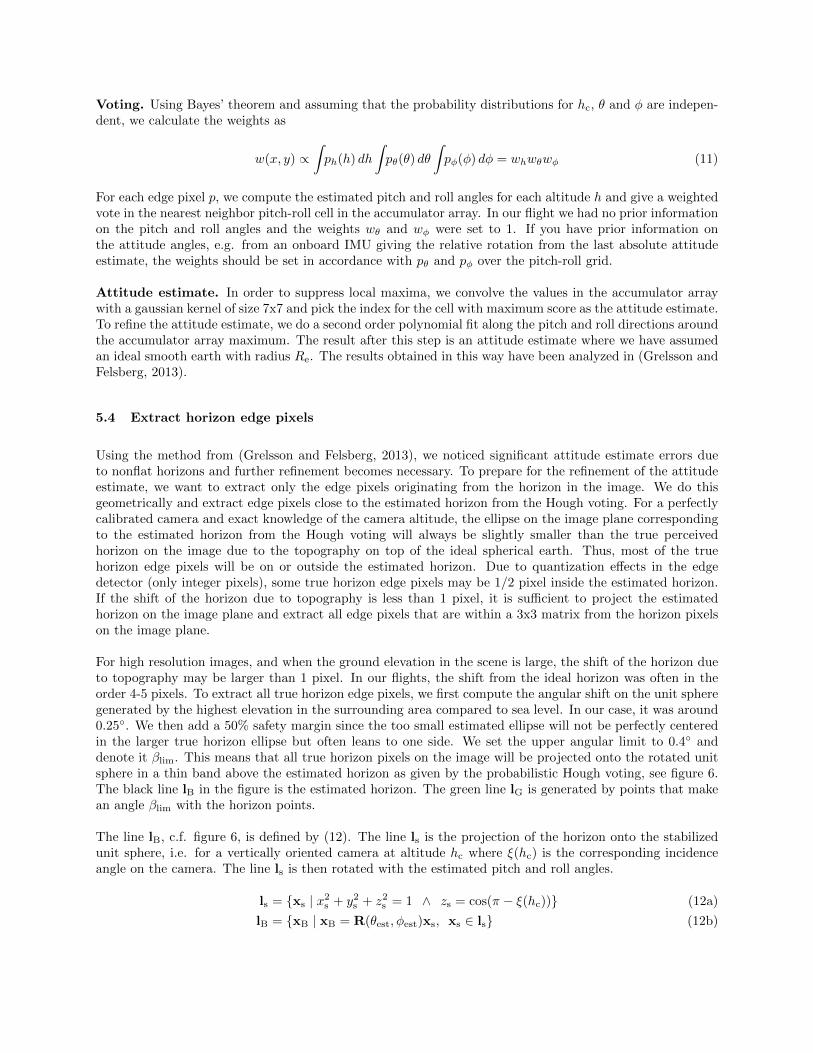
For high resolution images, and when the ground elevation in the scene is large, the shift of the horizon dueto topography may be larger than 1 pixel. In our flights, the shift from the ideal horizon was often in theorder 4-5 pixels. To extract all true horizon edge pixels, we first compute the angular shift on the unit spheregenerated by the highest elevation in the surrounding area compared to sea level. In our case, it was around0.25◦. We then add a 50% safety margin since the too small estimated ellipse will not be perfectly centeredin the larger true horizon ellipse but often leans to one side. We set the upper angular limit to 0.4◦ anddenote it βlim. This means that all true horizon pixels on the image will be projected onto the rotated unitsphere in a thin band above the estimated horizon as given by the probabilistic Hough voting, see figure 6.The black line lB in the figure is the estimated horizon. The green line lG is generated by points that makean angle βlim with the horizon points.
The line lB, c.f. figure 6, is defined by (12). The line ls is the projection of the horizon onto the stabilizedunit sphere, i.e. for a vertically oriented camera at altitude hc where ξ(hc) is the corresponding incidenceangle on the camera. The line ls is then rotated with the estimated pitch and roll angles.
ls = {xs | x2s + y2s + z2s = 1 ∧ zs = cos(π − ξ(hc))} (12a)
lB = {xB | xB = R(θest, φest)xs, xs ∈ ls} (12b)
x
z
y n
l B
l G
c
c c
Figure 6: Band on rotated unit sphere with conceivable true horizon edge pixels.
The line lG is defined by (13). Compared to ls, the line lsh is shifted an angle βlim upwards on the unitsphere.
lsh = {xsh | x2sh + y2sh + z2sh = 1 ∧ zsh = cos(π − ξ(hc)− βlim)} (13a)
lG = {xG | xG = R(θest, φest)xsh, xsh ∈ lsh} (13b)
We project the band between the lines lB and lG onto the image plane to create a mask for potential horizonedge pixels. Since the edge detector gives integer pixel values, we include a 3x3 neighborhood around eachprojection point on the image plane in the mask. From the Canny edge image, we only extract the edgepixels within the mask for the subsequent attitude refining process.
5.5 Compute geometrical horizon
To compute the geometrical horizon, the availability of a DEM is required. In our case, we use the SRTM3database, (NASA, 2013). See section 5.8.1 for more details. We also need an approximate global 3D positionfor the vehicle. This 3D position may be obtained from a GPS onboard the vehicle but it could equally wellbe estimated utilizing a ground terrain navigation method. These methods may be image based like the oneproposed in (Grelsson et al., 2013).
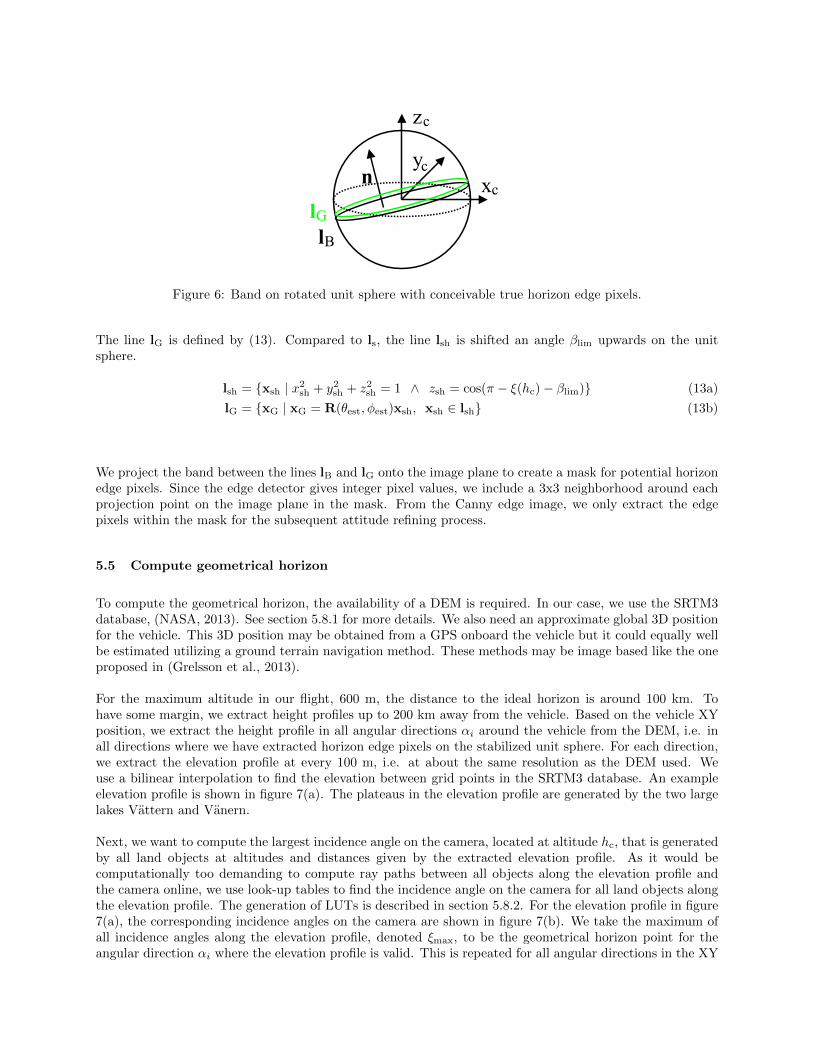
For the maximum altitude in our flight, 600 m, the distance to the ideal horizon is around 100 km. Tohave some margin, we extract height profiles up to 200 km away from the vehicle. Based on the vehicle XYposition, we extract the height profile in all angular directions αi around the vehicle from the DEM, i.e. inall directions where we have extracted horizon edge pixels on the stabilized unit sphere. For each direction,we extract the elevation profile at every 100 m, i.e. at about the same resolution as the DEM used. Weuse a bilinear interpolation to find the elevation between grid points in the SRTM3 database. An exampleelevation profile is shown in figure 7(a). The plateaus in the elevation profile are generated by the two largelakes Vattern and Vanern.
Next, we want to compute the largest incidence angle on the camera, located at altitude hc, that is generatedby all land objects at altitudes and distances given by the extracted elevation profile. As it would becomputationally too demanding to compute ray paths between all objects along the elevation profile andthe camera online, we use look-up tables to find the incidence angle on the camera for all land objects alongthe elevation profile. The generation of LUTs is described in section 5.8.2. For the elevation profile in figure7(a), the corresponding incidence angles on the camera are shown in figure 7(b). We take the maximum ofall incidence angles along the elevation profile, denoted ξmax, to be the geometrical horizon point for theangular direction αi where the elevation profile is valid. This is repeated for all angular directions in the XY
Figure 7: (a) Elevation profile and (b) corresponding incidence angle profile.
plane where we have horizon edge pixels on the stabilized unit sphere and results in a point set
wPgeom,i = [cosαi sinαi cos(π − ξmax,i)]T (14)
for the geometrically computed horizon.
5.6 Refine estimated attitude
The method we use for refining the estimated vehicle attitude may also be used for calibration of the cameraparameters and the camera mounting on the vehicle given that accurate position and attitudes are knownfrom other sensors. The difference is only which parameters are kept constant in a nonlinear optimizationprocess.
First, we denote the vehicle rotation matrix transforming points from a world coordinate frame to a vehiclebody frame as bwRveh and the corresponding camera rotation matrix as bwRc. Assuming that the camerais not perfectly aligned with the aircraft body, there is a relative rotation cvRrel between the vehicle frameand the camera frame defined as
cvRrel = bwRcbwRT
veh (15)
During the flight, the estimated vehicle orientation bwRveh,est is obtained from the estimated camera orien-tation bwRc,est as
bwRveh,est = cvRTrel
bwRc,est (16)
Now, we use the extracted horizon edge pixels in the image (described in section 5.4). We backproject allhorizon edge pixels onto the rotated unit sphere and denote the 3D point set on the sphere as bPs. Next, werotate the point set with the transpose of the estimated camera rotation matrix given by the probabilisticHough voting. The new rotated point set on the sphere
wPr = bwRTc,est
bPs = bwRTveh,est
cvRTrel
bPs (17)
will ideally be the perceived horizon points rotated to the stabilized unit sphere, i.e. a camera system alignedwith the world coordinate frame. With perfect image data, the rotated points wPr would correspond to thegeometrically computed horizon points wPgeom. Note that we need at least an approximate vehicle headingangle estimate which could be obtained e.g. from feature point tracking in the image sequence.
The induced error function is to minimize the sum of the arc lengths on the unit sphere between the respectivepoints in wPr and wPgeom. If we choose to compute the point set wPgeom for the angles
αi = tan−1(Pry,i/Prx,i) (18)
on the XY-plane, the small arcs between the point sets will have their main component along the z-axisof the unit sphere. Using a small arc angle approximation, we define the error function to be the squareddistance between the z-coordinate for the point sets, i.e.
εz =∑i
(Prz,i − Pgeomz,i)2 =
∑i
(Prz,i − cos(π − ξmax(αi)))2 (19)
where the summation is made over all extracted horizon edge points. For attitude refinement, we search forthe camera orientation bwRc that minimizes the error function in (19), i.e.
bwRc,est = argminbwRc
εz(bwRc). (20)
We minimize the error function using the Levenberg-Marquardt algorithm and initialize with the cameraorientation matrix from the Hough voting.
5.7 Camera calibration
If there is, as in our case, a ground truth available for the 3D world position and orientation for someimages, a similar scheme as for the attitude refinement may be used for calibration of the camera and itsmounting on the airborne vehicle. However, a good initialization for the camera parameters and the camerarotation matrix is required. Since this camera calibration is an off-line process, we start by selecting about10 images where, preferably, the extracted horizon edges are in good agreement with the visually expectedhorizon. Images are chosen where the horizon is located at different positions in the image, to improve theconditioning of the minimization problem.
One difference compared to the attitude refinement is that we now use the ground truth camera rotationmatrix bwRc,true to compute the rotated, backprojected points on the unit sphere.
wPr = bwRTc,true
bPs = bwRTveh,true
cvRTrel
bPs (21)
We minimize the same error function as in (19), but now sum over all horizon edge pixels in all of the chosenimages, i.e.
(bwRrel,est,Kest,Dest) = argminbwRrel,K,D
∑im
εz(im,bwRrel,K,D). (22)
Since we are now optimizing over 14 parameters in total, it is very likely that the Levenberg-Marquardtalgorithm will end up in a local minimum for the error function. Therefore, this process has shown toimprove the overall attitude estimation performance if a good initialization is provided.
5.8 DEM and LUT
5.8.1 Digital Elevation model
The DEM used in this paper is the freely available SRTM3 data from (NASA, 2013). The XY grid resolutionis 3 arc-seconds or around 90 m at the equator. The standard deviation for the elevation error is claimed tobe around 8 m.
5.8.2 Generation of LUT for topography
For a spherically stratified model (Gyer, 1996) shows that the angle θc from a ground point at altitude hgto the camera at altitude hc is given by
θc =
∫ hc
hg
k
r√n2r2 − k2
dr. (23)
R e
h i
n i ξ i
ξ
θ c
i-1
n i-1
n i+1 ξ
i+1
h i+1
i
r i r i+1
Ray path
(a)
R e
h c
d id
θ id
ξ c,id
h 0
(b)
R e
h c
d obj ξ c,obj
h obj h g
θ id
(c)
R e
h c
d 1 ξ c,obj
h obj
h 90
θ id
d 2
P obj
P c
P 90
(d)
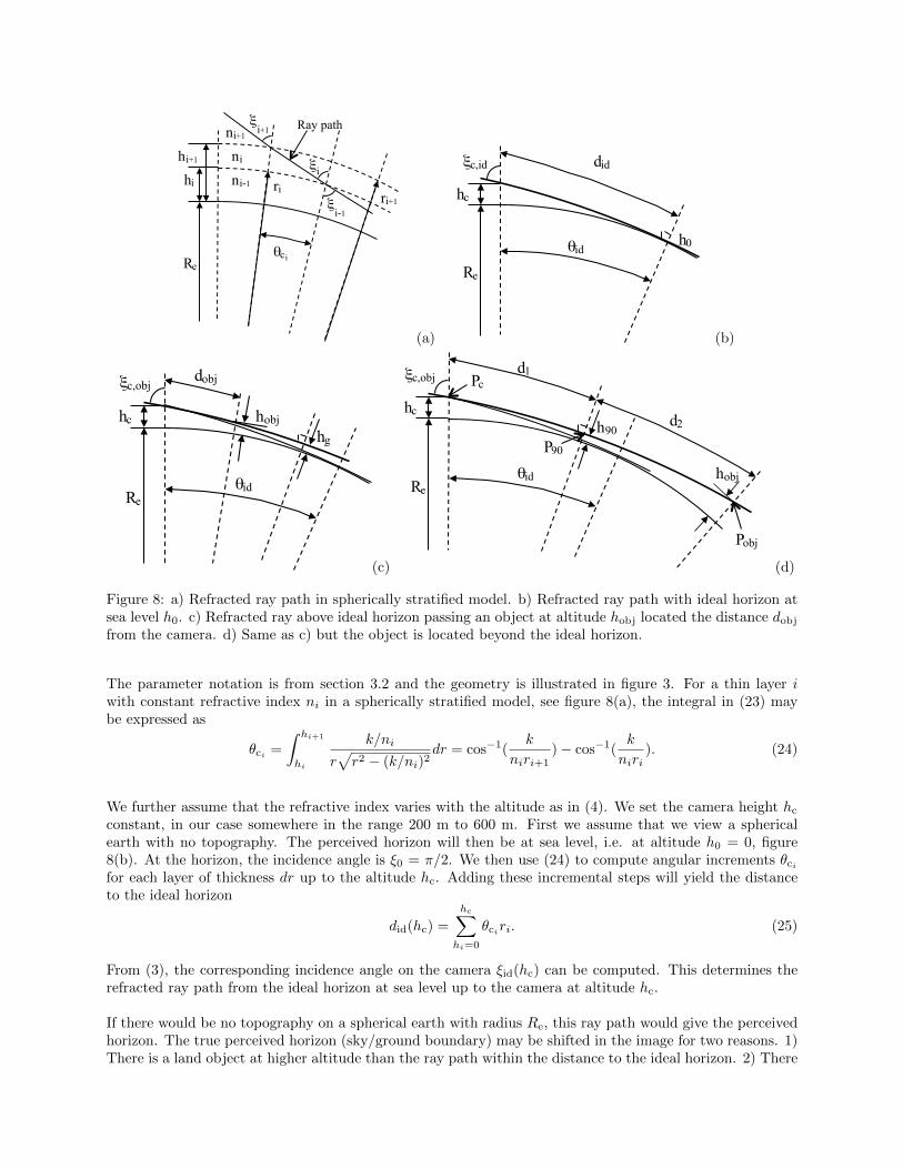
Figure 8: a) Refracted ray path in spherically stratified model. b) Refracted ray path with ideal horizon atsea level h0. c) Refracted ray above ideal horizon passing an object at altitude hobj located the distance dobjfrom the camera. d) Same as c) but the object is located beyond the ideal horizon.
The parameter notation is from section 3.2 and the geometry is illustrated in figure 3. For a thin layer iwith constant refractive index ni in a spherically stratified model, see figure 8(a), the integral in (23) maybe expressed as
θci =
∫ hi+1
hi
k/ni
r√r2 − (k/ni)2
dr = cos−1(k
niri+1)− cos−1(
k
niri). (24)
We further assume that the refractive index varies with the altitude as in (4). We set the camera height hcconstant, in our case somewhere in the range 200 m to 600 m. First we assume that we view a sphericalearth with no topography. The perceived horizon will then be at sea level, i.e. at altitude h0 = 0, figure8(b). At the horizon, the incidence angle is ξ0 = π/2. We then use (24) to compute angular increments θcifor each layer of thickness dr up to the altitude hc. Adding these incremental steps will yield the distanceto the ideal horizon
did(hc) =
hc∑hi=0
θciri. (25)
From (3), the corresponding incidence angle on the camera ξid(hc) can be computed. This determines therefracted ray path from the ideal horizon at sea level up to the camera at altitude hc.
If there would be no topography on a spherical earth with radius Re, this ray path would give the perceivedhorizon. The true perceived horizon (sky/ground boundary) may be shifted in the image for two reasons. 1)There is a land object at higher altitude than the ray path within the distance to the ideal horizon. 2) There

is a land object furher away than the distance to the ideal horizon, but at sufficent height to be perceivedat an incidence angle above the ideal horizon.
High objects within distance to ideal horizon. To compute this effect, consider a ground height hgbetween 0 and hc. Set the incidence angle at the ground object ξg = π/2. Compute the ray path in thesame manner as above until it reaches the altitude hc. Extract data points from the ray path at desired landobject heights hobj and record the corresponding distances to the camera dc,obj and the ray incidence angleon the camera ξobj, see figure 8(c). Repeat the computations for all ground heights hg from 0 to hc in steps∆hg.
High objects beyond distance to ideal horizon. Even if an object is further away from the camerathan the distance to the ideal horizon, the object may shift the sky/ground limit from the ideal case. Theray from the camera may take a path as in figure 8(d) where the ray starts at point Pobj, lowers in altitudefrom the ground object until it reaches the incidence angle π/2 at point P90 and then increases in altitudeagain until it reaches the camera at point Pc. To compute this effect, we start with a ray at altitude h90 andset the incidence angle ξ90 = π/2. We compute the ray path up to the maximum of the camera height hcand the highest object height hobj,max in the DEM. From this ray path, extract the distance to the camera dlfrom P90 and the corresponding ray incidence angle on the camera ξc,obj. From the ray path on the right sideof P90, extract the distances dr to the desired object heights hobj. Sum the distances d1 and d2 to obtain thetotal distance dobj from the camera to the object at height hobj and record together with the correspondingincidence angle ξobj. Repeat the computations for the altitude h90 from 0 up to hc.
From the two cases 1 and 2, we can now extract for each camera height hc and object height hobj, a pointset with incidence angles and distances from the camera to the object. We resample this point set to obtainincidence angles at the desired step size for the distance, in our case at every 100 m up to 200 km. Wegenerated LUTs where the input parameters are camera height (increment 2 m), object height (increment 2m), distance from camera (increment 100 m) and the output parameter is the incidence angle on the camera.
We have only considered objects that are at a higher altitude than the camera if the objects are beyond thedistance to the ideal horizon. The reason is that for the images considered in our test flight, there were noobjects at a higher altitude than the camera within the distance to the ideal horizon.
6 Flight trial
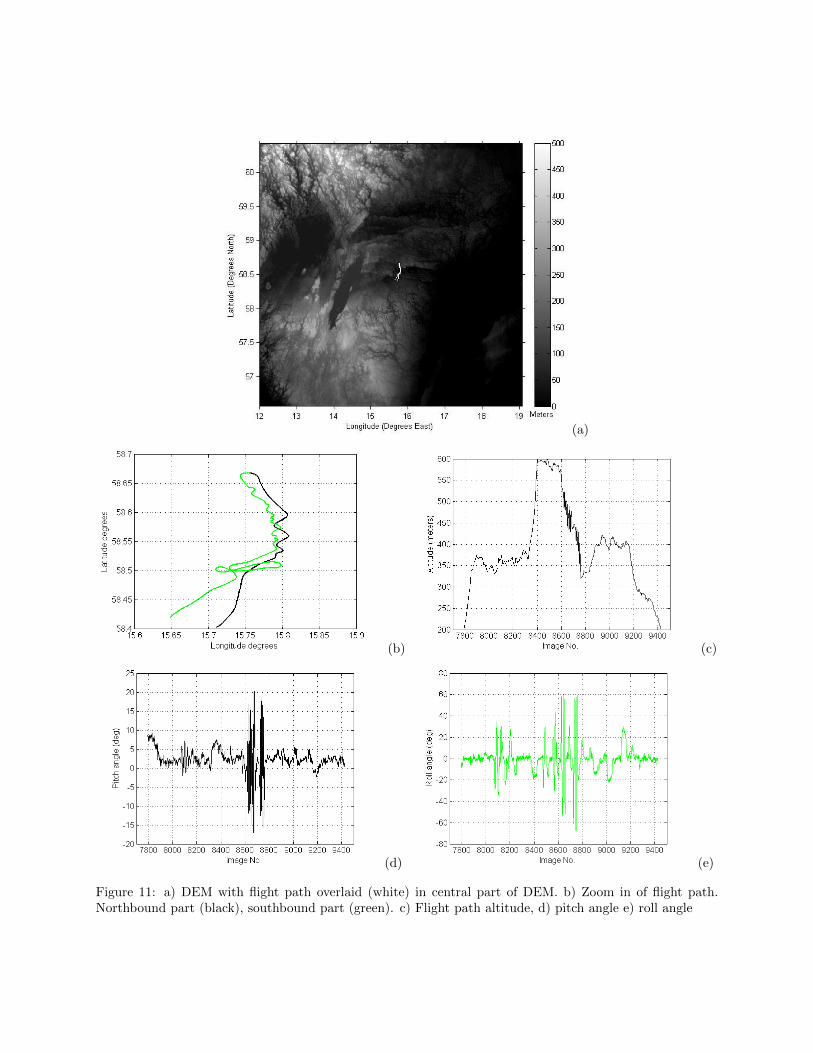
To evaluate the proposed attitude estimation method, an aircraft flight trial with a fisheye lens camera wasperformed. A Nikon D800 with a Sigma f/8mm lens was mounted below the aircraft, figure 9. The imageresolution is 6144x4912 pixels. The field-of-view is around 183◦ resulting in a resolution around 0.04◦/pxfor the full resolution images. For ease of camera mounting, the camera optical axis was not vertical butdirected roughly 10◦ to the right (starboard) and 10◦ backwards (aft). This implies that when the aircraftwas in level flight, the horizon was seen starboard (down in image) and aft (left in image) of the aircraft asshown in figure 10.
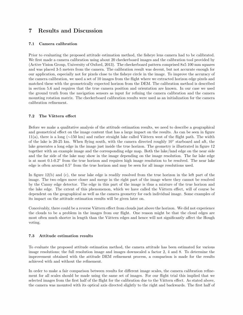
The flight was carried out around Linkoping in Sweden, see map in figure 11 a)-b), with ground elevationsfrom sea surface up to around 500 m within a 200 km radius from the aircraft. Images were captured ataround 1 fps with flight altitudes up to 600 m. The flight lasted for about 30 minutes and 1629 images werecaptured from 200 m altitude and above. These images are numbered 7795 to 9423 in the sequel. The flightaltitude and the pitch and roll angles during flight are shown in figure 11 c)-e).
Flight data was also recorded with a GPS and a highly accurate (tactical grade) IMU. The navigation sensorsystem used was a POS AV 510 from Applanix (Applanix, 2014). The ground truth 6DOF pose for theaircraft during the flight was obtained from an offline filtering process having navigation data from thecomplete flight available. A forward and backward filtering process was employed implying that the ground
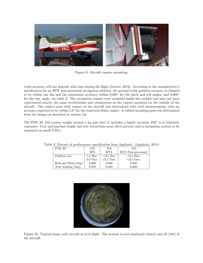
Figure 9: Aircraft camera mounting.
truth accuracy will not degrade with time during the flight (Groves, 2013). According to the manufacturer’sspecification for an RTX post-processed navigation solution, the ground truth position accuracy is claimedto be within one dm and the orientation accuracy within 0.005◦ for the pitch and roll angles, and 0.008◦
for the yaw angle, see table 2. The navigation sensors were mounted inside the cockpit and may not haveexperienced exactly the same accelerations and orientations as the camera mounted on the outside of theaircraft. The camera pose with respect to the aircraft was determined with level measurements, with anaccuracy expected to be within 1.0◦ for the respective Euler angles. A refined mounting pose was determinedfrom the images as described in section 5.6.
The POS AV 510 system weighs around 4 kg and since it includes a highly accurate IMU it is relativelyexpensive. Cost and payload weight and size restrictions most often prevent such a navigation system to beemployed on small UAVs.
Table 2: Extract of performance specification from Applanix. (Applanix, 2014)POS AV 510 510 510
SPS RTX RTX Post-processed
Position (m) 1.5 Hor. <0.1 Hor <0.1 Hor.3.0 Vert. <0.2 Vert. <0.2 Vert.
Roll and Pitch (deg) 0.008 0.008 0.005True heading (deg) 0.070 0.040 0.008
Figure 10: Typical image with aircraft in level flight. The horizon is seen starboard (down) and aft (left) ofthe aircraft.
(a)
(b) (c)
(d) (e)
Figure 11: a) DEM with flight path overlaid (white) in central part of DEM. b) Zoom in of flight path.Northbound part (black), southbound part (green). c) Flight path altitude, d) pitch angle e) roll angle
7 Results and Discussion
7.1 Camera calibration
Prior to evaluating the proposed attitude estimation method, the fisheye lens camera had to be calibrated.We first made a camera calibration using about 20 checkerboard images and the calibration tool provided by(Active Vision Group, University of Oxford, 2013). The checkerboard pattern comprised 8x5 100 mm squaresand was placed 3-5 meters from the camera. The calibration result was decent, but not accurate enough forour application, especially not for pixels close to the fisheye circle in the image. To improve the accuracy ofthe camera calibration, we used a set of 10 images from the flight where we extracted horizon edge pixels andmatched these with the geometrically expected horizon from the DEM. The calibration method is describedin section 5.6 and requires that the true camera position and orientation are known. In our case we usedthe ground truth from the navigation sensors as input for refining the camera calibration and the cameramounting rotation matrix. The checkerboard calibration results were used as an initialization for the cameracalibration refinement.
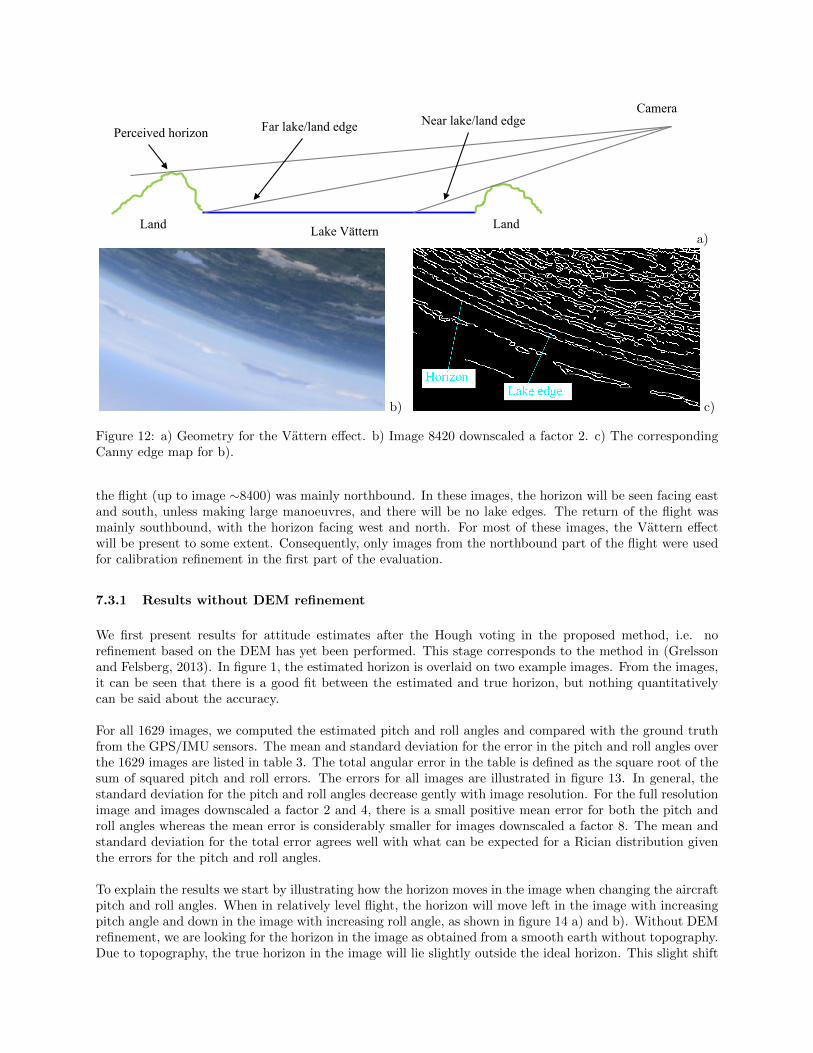
7.2 The Vattern effect
Before we make a qualitative analysis of the attitude estimation results, we need to describe a geographicaland geometrical effect on the image content that has a large impact on the results. As can be seen in figure11(a), there is a long (∼150 km) and rather straight lake called Vattern west of the flight path. The widthof the lake is 20-25 km. When flying south, with the camera directed roughly 10◦ starboard and aft, thelake generates a long edge in the image just inside the true horizon. The geometry is illustrated in figure 12together with an example image and the corresponding edge map. Both the lake/land edge on the near sideand the far side of the lake may show in the image depending on the image resolution. The far lake edgeis at most 0.1-0.2◦ from the true horizon and requires high image resolution to be resolved. The near lakeedge is often around 0.5◦ from the true horizon and may be seen for all image resolutions used.
In figure 12(b) and (c), the near lake edge is readily resolved from the true horizon in the left part of theimage. The two edges move closer and merge in the right part of the image where they cannot be resolvedby the Canny edge detector. The edge in this part of the image is thus a mixture of the true horizon andthe lake edge. The extent of this phenomenon, which we have called the Vattern effect, will of course bedependent on the geographical as well as the camera geometry for each individual image. Some examples ofits impact on the attitude estimation results will be given later on.
Conceivably, there could be a reverse Vattern effect from clouds just above the horizon. We did not experiencethe clouds to be a problem in the images from our flight. One reason might be that the cloud edges aremost often much shorter in length than the Vattern edges and hence will not significantly affect the Houghvoting.
7.3 Attitude estimation results
To evaluate the proposed attitude estimation method, the camera attitude has been estimated for variousimage resolutions; the full resolution image and images downscaled a factor 2, 4 and 8. To determine theimprovement obtained with the attitude DEM refinement process, a comparison is made for the resultsachieved with and without the refinement.
In order to make a fair comparison between results for different image scales, the camera calibration refine-ment for all scales should be made using the same set of images. For our flight trial this implied that weselected images from the first half of the flight for the calibration due to the Vattern effect. As stated above,the camera was mounted with its optical axis directed slightly to the right and backwards. The first half of
Camera
Lake Vättern
Perceived horizon Near lake/land edge
Land Land
Far lake/land edge
a)
b) c)
Figure 12: a) Geometry for the Vattern effect. b) Image 8420 downscaled a factor 2. c) The correspondingCanny edge map for b).
the flight (up to image ∼8400) was mainly northbound. In these images, the horizon will be seen facing eastand south, unless making large manoeuvres, and there will be no lake edges. The return of the flight wasmainly southbound, with the horizon facing west and north. For most of these images, the Vattern effectwill be present to some extent. Consequently, only images from the northbound part of the flight were usedfor calibration refinement in the first part of the evaluation.
7.3.1 Results without DEM refinement
We first present results for attitude estimates after the Hough voting in the proposed method, i.e. norefinement based on the DEM has yet been performed. This stage corresponds to the method in (Grelssonand Felsberg, 2013). In figure 1, the estimated horizon is overlaid on two example images. From the images,it can be seen that there is a good fit between the estimated and true horizon, but nothing quantitativelycan be said about the accuracy.
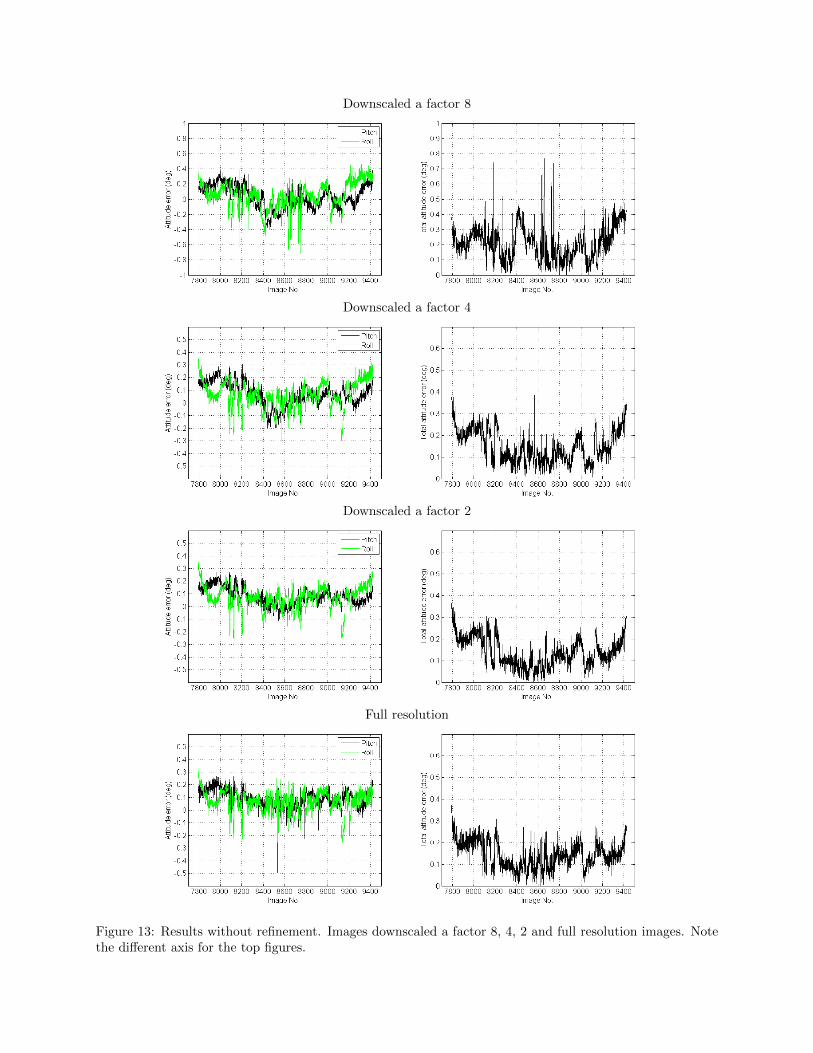
For all 1629 images, we computed the estimated pitch and roll angles and compared with the ground truthfrom the GPS/IMU sensors. The mean and standard deviation for the error in the pitch and roll angles overthe 1629 images are listed in table 3. The total angular error in the table is defined as the square root of thesum of squared pitch and roll errors. The errors for all images are illustrated in figure 13. In general, thestandard deviation for the pitch and roll angles decrease gently with image resolution. For the full resolutionimage and images downscaled a factor 2 and 4, there is a small positive mean error for both the pitch androll angles whereas the mean error is considerably smaller for images downscaled a factor 8. The mean andstandard deviation for the total error agrees well with what can be expected for a Rician distribution giventhe errors for the pitch and roll angles.
To explain the results we start by illustrating how the horizon moves in the image when changing the aircraftpitch and roll angles. When in relatively level flight, the horizon will move left in the image with increasingpitch angle and down in the image with increasing roll angle, as shown in figure 14 a) and b). Without DEMrefinement, we are looking for the horizon in the image as obtained from a smooth earth without topography.Due to topography, the true horizon in the image will lie slightly outside the ideal horizon. This slight shift
Downscaled a factor 8
Downscaled a factor 4
Downscaled a factor 2
Full resolution
Figure 13: Results without refinement. Images downscaled a factor 8, 4, 2 and full resolution images. Notethe different axis for the top figures.
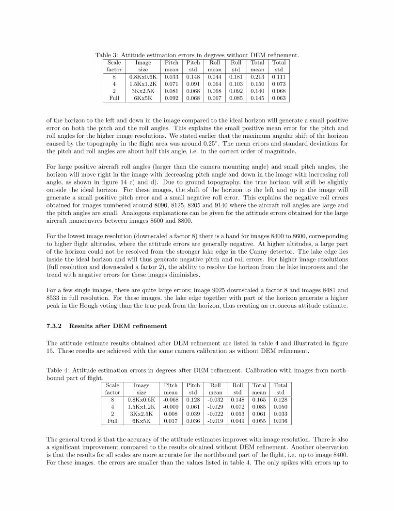
Table 3: Attitude estimation errors in degrees without DEM refinement.Scale Image Pitch Pitch Roll Roll Total Totalfactor size mean std mean std mean std
8 0.8Kx0.6K 0.033 0.148 0.044 0.181 0.213 0.1114 1.5Kx1.2K 0.071 0.091 0.064 0.103 0.150 0.0732 3Kx2.5K 0.081 0.068 0.068 0.092 0.140 0.068
Full 6Kx5K 0.092 0.068 0.067 0.085 0.145 0.063
of the horizon to the left and down in the image compared to the ideal horizon will generate a small positiveerror on both the pitch and the roll angles. This explains the small positive mean error for the pitch androll angles for the higher image resolutions. We stated earlier that the maximum angular shift of the horizoncaused by the topography in the flight area was around 0.25◦. The mean errors and standard deviations forthe pitch and roll angles are about half this angle, i.e. in the correct order of magnitude.
For large positive aircraft roll angles (larger than the camera mounting angle) and small pitch angles, thehorizon will move right in the image with decreasing pitch angle and down in the image with increasing rollangle, as shown in figure 14 c) and d). Due to ground topography, the true horizon will still be slightlyoutside the ideal horizon. For these images, the shift of the horizon to the left and up in the image willgenerate a small positive pitch error and a small negative roll error. This explains the negative roll errorsobtained for images numbered around 8090, 8125, 8205 and 9140 where the aircraft roll angles are large andthe pitch angles are small. Analogous explanations can be given for the attitude errors obtained for the largeaircraft manoeuvres between images 8600 and 8800.
For the lowest image resolution (downscaled a factor 8) there is a band for images 8400 to 8600, correspondingto higher flight altitudes, where the attitude errors are generally negative. At higher altitudes, a large partof the horizon could not be resolved from the stronger lake edge in the Canny detector. The lake edge liesinside the ideal horizon and will thus generate negative pitch and roll errors. For higher image resolutions(full resolution and downscaled a factor 2), the ability to resolve the horizon from the lake improves and thetrend with negative errors for these images diminishes.
For a few single images, there are quite large errors; image 9025 downscaled a factor 8 and images 8481 and8533 in full resolution. For these images, the lake edge together with part of the horizon generate a higherpeak in the Hough voting than the true peak from the horizon, thus creating an erroneous attitude estimate.
7.3.2 Results after DEM refinement
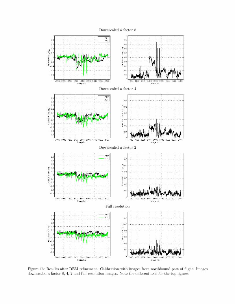
The attitude estimate results obtained after DEM refinement are listed in table 4 and illustrated in figure15. These results are achieved with the same camera calibration as without DEM refinement.
Table 4: Attitude estimation errors in degrees after DEM refinement. Calibration with images from north-bound part of flight.
Scale Image Pitch Pitch Roll Roll Total Totalfactor size mean std mean std mean std
8 0.8Kx0.6K -0.068 0.128 -0.032 0.148 0.165 0.1284 1.5Kx1.2K -0.009 0.061 -0.029 0.072 0.085 0.0502 3Kx2.5K 0.008 0.039 -0.022 0.053 0.061 0.033
Full 6Kx5K 0.017 0.036 -0.019 0.049 0.055 0.036
The general trend is that the accuracy of the attitude estimates improves with image resolution. There is alsoa significant improvement compared to the results obtained without DEM refinement. Another observationis that the results for all scales are more accurate for the northbound part of the flight, i.e. up to image 8400.For these images. the errors are smaller than the values listed in table 4. The only spikes with errors up to
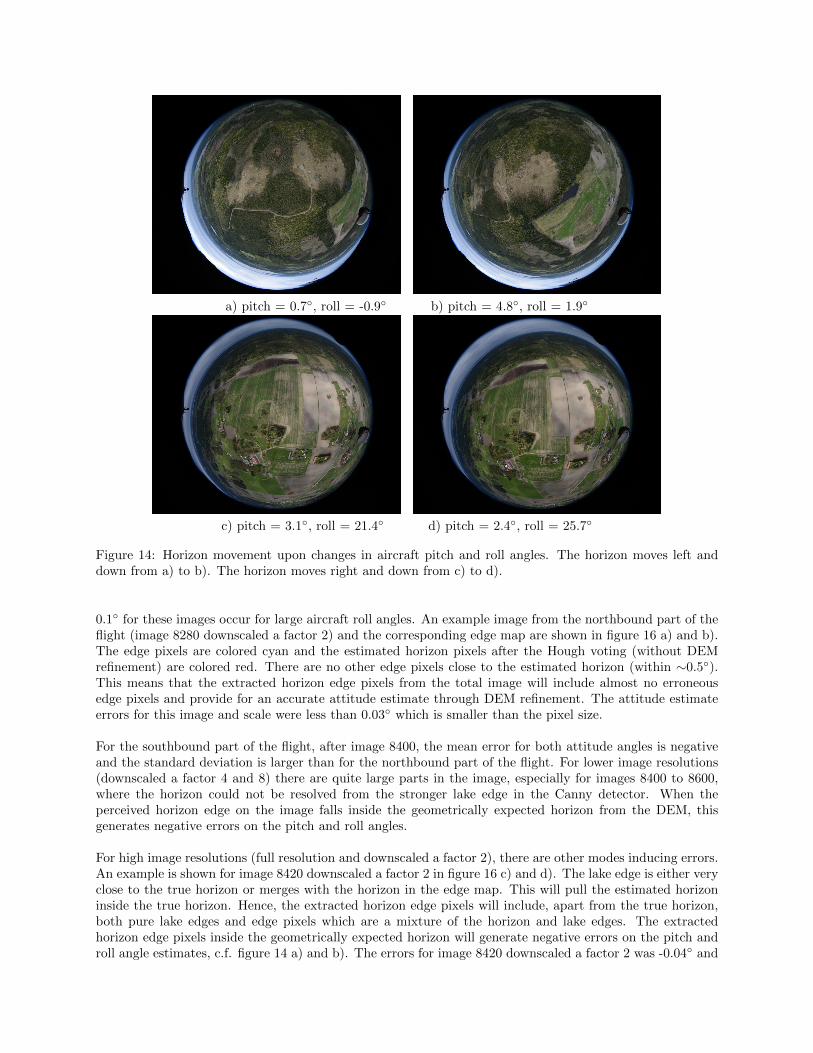
a) pitch = 0.7◦, roll = -0.9◦ b) pitch = 4.8◦, roll = 1.9◦
c) pitch = 3.1◦, roll = 21.4◦ d) pitch = 2.4◦, roll = 25.7◦
Figure 14: Horizon movement upon changes in aircraft pitch and roll angles. The horizon moves left anddown from a) to b). The horizon moves right and down from c) to d).
0.1◦ for these images occur for large aircraft roll angles. An example image from the northbound part of theflight (image 8280 downscaled a factor 2) and the corresponding edge map are shown in figure 16 a) and b).The edge pixels are colored cyan and the estimated horizon pixels after the Hough voting (without DEMrefinement) are colored red. There are no other edge pixels close to the estimated horizon (within ∼0.5◦).This means that the extracted horizon edge pixels from the total image will include almost no erroneousedge pixels and provide for an accurate attitude estimate through DEM refinement. The attitude estimateerrors for this image and scale were less than 0.03◦ which is smaller than the pixel size.
For the southbound part of the flight, after image 8400, the mean error for both attitude angles is negativeand the standard deviation is larger than for the northbound part of the flight. For lower image resolutions(downscaled a factor 4 and 8) there are quite large parts in the image, especially for images 8400 to 8600,where the horizon could not be resolved from the stronger lake edge in the Canny detector. When theperceived horizon edge on the image falls inside the geometrically expected horizon from the DEM, thisgenerates negative errors on the pitch and roll angles.
For high image resolutions (full resolution and downscaled a factor 2), there are other modes inducing errors.An example is shown for image 8420 downscaled a factor 2 in figure 16 c) and d). The lake edge is either veryclose to the true horizon or merges with the horizon in the edge map. This will pull the estimated horizoninside the true horizon. Hence, the extracted horizon edge pixels will include, apart from the true horizon,both pure lake edges and edge pixels which are a mixture of the horizon and lake edges. The extractedhorizon edge pixels inside the geometrically expected horizon will generate negative errors on the pitch androll angle estimates, c.f. figure 14 a) and b). The errors for image 8420 downscaled a factor 2 was -0.04◦ and
Downscaled a factor 8
Downscaled a factor 4
Downscaled a factor 2
Full resolution
Figure 15: Results after DEM refinement. Calibration with images from northbound part of flight. Imagesdownscaled a factor 8, 4, 2 and full resolution images. Note the different axis for the top figures.

a) b)
c) d)
e) f)
Figure 16: Images and Canny edge maps (cyan) with estimated horizon after Hough voting overlaid (red).Image 8280 downscaled a factor 2 a),b), image 8420 downscaled a factor 2 c),d), image 8913 in full resolutione),f).
-0.15◦ for the pitch and roll angles respectively.
Another example is image 8913 in full resolution shown in figure 16 e) and f). Here, the lake edge and thetrue horizon can be seen as almost parallel edges separated around 0.15◦. The estimated horizon assumingan ideal earth, which has a smaller radius than the true horizon, almost coincides with the lake edge in thiszoomed part of the total image. Hence, when extracting horizon edge pixels, both the lake edges and thetrue horizon edges will be included. The lake edges lie inside the geometrically expected horizon and willinduce negative errors on the pitch and roll angle estimates. In this case the errors were -0.04◦ and -0.14◦
for the pitch and roll angles.
For image 8533 in full resolution, the error mode is the same as for image 8913, with a long lake edge insidethe true horizon. But, in addition, haze in the image conceals and denies the detection of an edge for thetrue horizon in quite a large part of the image. In total, this means that when extracting horizon edge pixels,a very large fraction of lake edges are included generating a total angular error around 0.6◦.
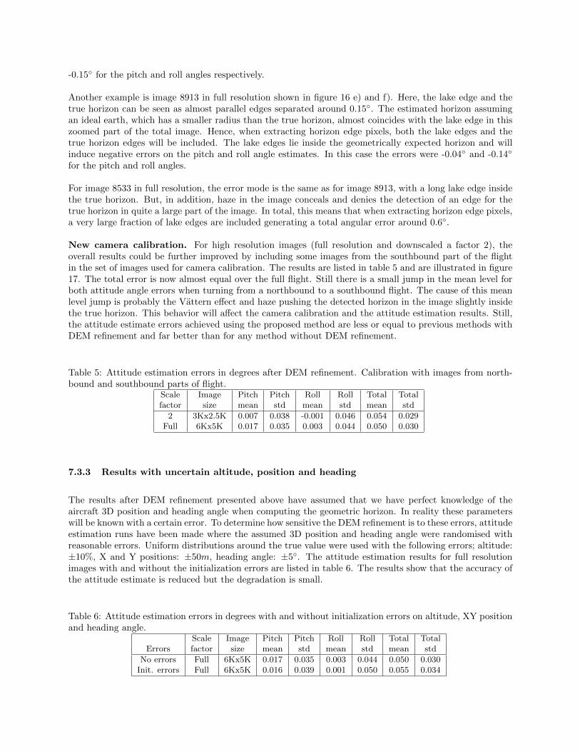
New camera calibration. For high resolution images (full resolution and downscaled a factor 2), theoverall results could be further improved by including some images from the southbound part of the flightin the set of images used for camera calibration. The results are listed in table 5 and are illustrated in figure17. The total error is now almost equal over the full flight. Still there is a small jump in the mean level forboth attitude angle errors when turning from a northbound to a southbound flight. The cause of this meanlevel jump is probably the Vattern effect and haze pushing the detected horizon in the image slightly insidethe true horizon. This behavior will affect the camera calibration and the attitude estimation results. Still,the attitude estimate errors achieved using the proposed method are less or equal to previous methods withDEM refinement and far better than for any method without DEM refinement.
Table 5: Attitude estimation errors in degrees after DEM refinement. Calibration with images from north-bound and southbound parts of flight.
Scale Image Pitch Pitch Roll Roll Total Totalfactor size mean std mean std mean std
2 3Kx2.5K 0.007 0.038 -0.001 0.046 0.054 0.029Full 6Kx5K 0.017 0.035 0.003 0.044 0.050 0.030
7.3.3 Results with uncertain altitude, position and heading
The results after DEM refinement presented above have assumed that we have perfect knowledge of theaircraft 3D position and heading angle when computing the geometric horizon. In reality these parameterswill be known with a certain error. To determine how sensitive the DEM refinement is to these errors, attitudeestimation runs have been made where the assumed 3D position and heading angle were randomised withreasonable errors. Uniform distributions around the true value were used with the following errors; altitude:±10%, X and Y positions: ±50m, heading angle: ±5◦. The attitude estimation results for full resolutionimages with and without the initialization errors are listed in table 6. The results show that the accuracy ofthe attitude estimate is reduced but the degradation is small.
Table 6: Attitude estimation errors in degrees with and without initialization errors on altitude, XY positionand heading angle.
Scale Image Pitch Pitch Roll Roll Total TotalErrors factor size mean std mean std mean std
No errors Full 6Kx5K 0.017 0.035 0.003 0.044 0.050 0.030Init. errors Full 6Kx5K 0.016 0.039 0.001 0.050 0.055 0.034
Downscaled a factor 2
Full resolution
Figure 17: Results after DEM refinement with new camera calibration. Images downscaled a factor 2 andfull resolution.
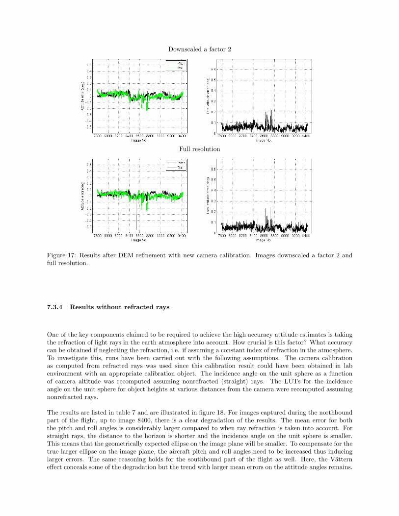
7.3.4 Results without refracted rays
One of the key components claimed to be required to achieve the high accuracy attitude estimates is takingthe refraction of light rays in the earth atmosphere into account. How crucial is this factor? What accuracycan be obtained if neglecting the refraction, i.e. if assuming a constant index of refraction in the atmosphere.To investigate this, runs have been carried out with the following assumptions. The camera calibrationas computed from refracted rays was used since this calibration result could have been obtained in labenvironment with an appropriate calibration object. The incidence angle on the unit sphere as a functionof camera altitude was recomputed assuming nonrefracted (straight) rays. The LUTs for the incidenceangle on the unit sphere for object heights at various distances from the camera were recomputed assumingnonrefracted rays.
The results are listed in table 7 and are illustrated in figure 18. For images captured during the northboundpart of the flight, up to image 8400, there is a clear degradation of the results. The mean error for boththe pitch and roll angles is considerably larger compared to when ray refraction is taken into account. Forstraight rays, the distance to the horizon is shorter and the incidence angle on the unit sphere is smaller.This means that the geometrically expected ellipse on the image plane will be smaller. To compensate for thetrue larger ellipse on the image plane, the aircraft pitch and roll angles need to be increased thus inducinglarger errors. The same reasoning holds for the southbound part of the flight as well. Here, the Vatterneffect conceals some of the degradation but the trend with larger mean errors on the attitude angles remains.
Table 7: Attitude estimation errors in degrees with and without refracted rays.Scale Image Pitch Pitch Roll Roll Total Total
Rays factor size mean std mean std mean std
Refracted Full 6Kx5K 0.017 0.035 0.003 0.044 0.050 0.030Straight Full 6Kx5K 0.049 0.036 0.040 0.053 0.085 0.034
Figure 18: Results after DEM refinement assuming straight rays.
7.3.5 Error analysis
The results presented above have shown that after DEM refinement the mean error for the estimated pitchand roll angles is smaller than the pixel resolution (which is 0.04◦) and the standard deviation for the errorsis in the same order as the pixel resolution. Is the accuracy obtained quantitatively reasonable and whatare the factors determining the accuracy? The main error sources in our flight trial are explained below andsummarized in table 8.
Table 8: Error sources and their impact on the attitude estimates.Error source Error (deg) Comments
Ground truth accuracy 0.01DEM resolution and accuracy ∼0.01 Larger errors in hilly terrainRay refraction <0.01 Offset errors 0.05◦-0.10◦ if ray refraction is ignoredImage scene content 0 - 0.2 Often close to zero, in rare cases (lake edges) up to 0.2◦
Camera calibration 0.01-0.02 Depend on ground truth and DEM accuracy
Ground truth accuracy. The accuracy of the ground truth orientation from the navigation sensorsis claimed to be around 0.01◦ for all attitude angles. The uncertainty measure for the filtered solutionvaries during flight depending on the excitation of the gyros and IMUs. As previously stated, the navigationsensors were placed inside cock-pit whereas the camera was mounted below the aircraft. This means that thenavigation sensors and the camera may not experience exactly the same forces and their relative orientationmay differ slightly during flight. This may be one of the reasons that the largest errors for the attitudeestimates coincide with large aircraft maneuvers.
DEM resolution and accuracy. The DEM used to compute the geometrically expected horizon is theSRTM3 database where elevations are given for a 90x90 m grid on the ground. The SRTM3 data wasgenerated from satellite radar measurements. The radar measures an average of the altitude within an XYgrid cell, and it also measures an average between reflections from the ground and overlaying structures asroofs or treetops. This is not ideal when computing a geometrical horizon from an airborne visual sensor.It would be more appropriate to use a DEM containing the maximum elevation within each cell since thisis what a visual sensor will perceive as the horizon. However, this type of DEM is rarely available withlarge area coverage. The standard deviation for the SRTM3 elevations is claimed to be around 8 m. Due to
elevation variations within the grid cell, the difference between the maximum and the mean elevations caneasily be around 20 m in hilly terrain whereas the two values coincide for level ground. To illustrate theimpact of this elevation uncertainty on the attitude estimate we use a numerical example. For an aircraftflying at 400 m altitude, changing the ground elevation at the horizon from 200 m to 220 m generates a shiftof the perceived horizon that is close to 0.01◦.
Ray refraction. In section 7.3.4 it was shown how the accuracy of the attitude estimates was degraded if rayrefraction in the atmosphere was not taken into account. A spherically stratified model for the variation ofthe refractive index with altitude was used. The model assumes that the air pressure and temperature varieswith the altitude above the ground in a standardized manner. This is a first order approximation and doesnot take into account local variations in air pressure and temperature. However, since the difference betweenrefracted rays and straight rays generated an attitude estimate shift around 0.05◦, it seems reasonable thatthe deviation from the first order approximation generates errors that are smaller than 0.01◦.
Image scene content. Depending on the scene, this may be the largest source of error. A typical exampleis the Vattern effect where lake edges in the image interfere strongly with the detection of the true horizon.Lake edges, or edges from other objects in the scene, may conceal or merge with the true horizon in theimage. We are then dealing with local shifts in the perceived horizon that amounts to several pixels. Forour full image resolution this translates to errors in the order of 0.1-0.2◦.
Weather phenomena like presence of haze or fog may also induce errors on the horizon detection, and in turnon the attitude estimates. In our flight there was haze when looking in the west-northwest direction. Thismakes the perceived horizon more diffuse in the images and it may shift the location of the horizon edge inthe Canny detector slightly. The effect of haze is more pronounced at higher altitudes since then the lightrays need to propagate a longer distance through air to reach the horizon. We have no quantitative estimateof the errors induced by haze on the attitude estimates.
Camera calibration. In our case we used ground truth orientation data and elevation data from the DEMto refine the camera calibration, both the intrinsic parameters and the camera mounting on the aircraft frame.Even if we carefully select images where the image scene content does not introduce erroneous edges, theerrors from the ground truth and the DEM combined accumulate to 0.01-0.02◦. These errors will inevitablygenerate small errors on the camera calibration.
The camera calibration includes a nonlinear optimization to find a total of 14 intrinsic and extrinsic cameraparameters. It was evident that different camera calibrations were obtained depending on the image set usedfor calibration and also the initialization values in the nonlinear optimization. However, evaluations showedthat very similar overall attitude estimation results were obtained for slightly different camera calibrations.
Total error. When adding the errors from the camera calibration and the DEM, error propagation willlead to total attitude estimate errors in the order 0.02-0.03◦. This is also very close to the accuracy thatwas actually achieved with the proposed method for the full resolution images. The somewhat larger errorsthat were obtained can probably be attributed to the images where the Vattern effect was evident. Tofurther improve the results, either a more accurate camera calibration method or a DEM with finer grid cellsize and higher elevation accuracy than provided by SRTM3 is required. The error analysis also explainswhy the attitude estimates are not significantly better for the full resolution images compared with imagesdownscaled a factor 2, c.f. table 5.
7.4 Implementation and processing times
The first four algorithmic steps in our method, c.f. figure 4, are coded in C++, where the OpenCV imple-mentations of the Canny detector and the Hough circle detector have been used as a base. The last twosteps in the algorithm as well as the camera calibration refinement are written in Matlab. Processing timesfor different image scales are listed in table 9. The processing times reported are valid for a standard laptop,
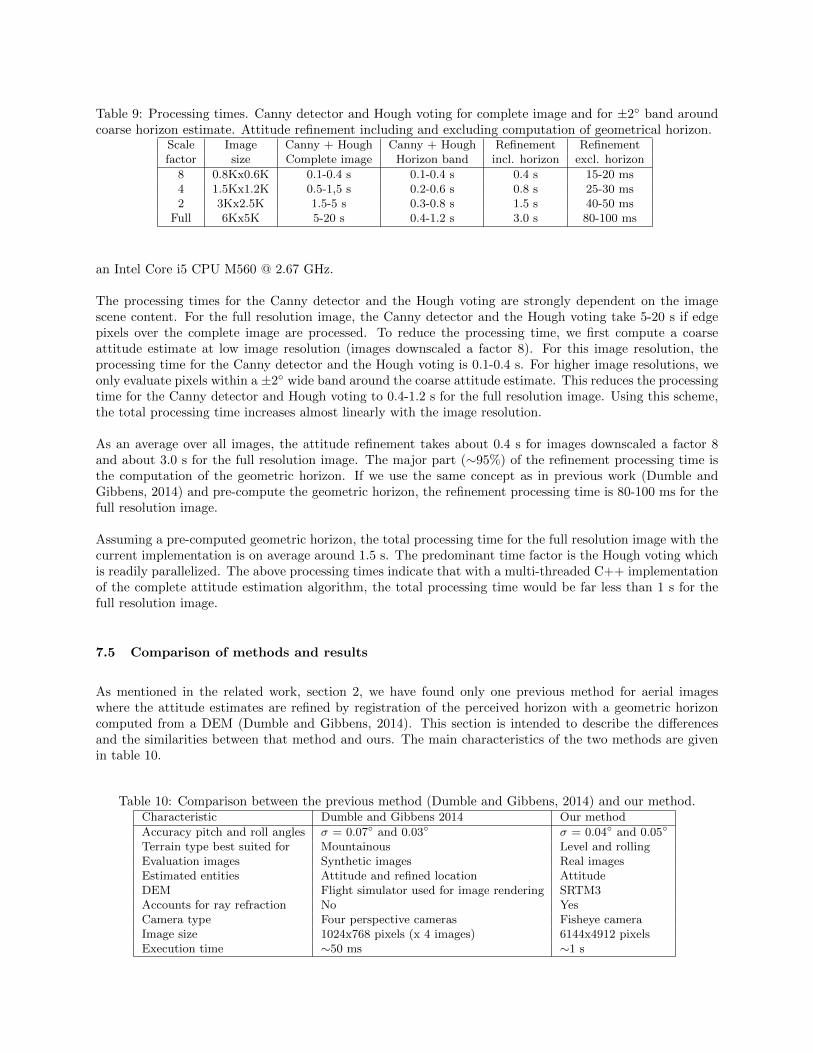
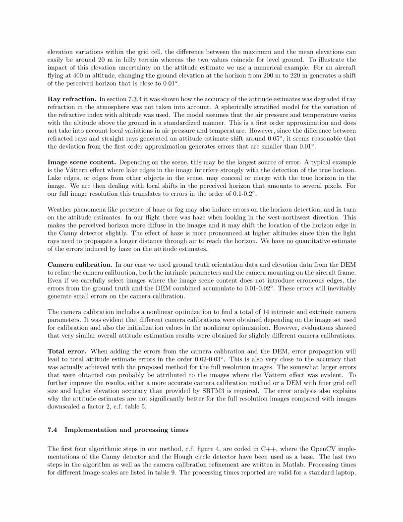
Table 9: Processing times. Canny detector and Hough voting for complete image and for ±2◦ band aroundcoarse horizon estimate. Attitude refinement including and excluding computation of geometrical horizon.
Scale Image Canny + Hough Canny + Hough Refinement Refinementfactor size Complete image Horizon band incl. horizon excl. horizon
8 0.8Kx0.6K 0.1-0.4 s 0.1-0.4 s 0.4 s 15-20 ms4 1.5Kx1.2K 0.5-1,5 s 0.2-0.6 s 0.8 s 25-30 ms2 3Kx2.5K 1.5-5 s 0.3-0.8 s 1.5 s 40-50 ms
Full 6Kx5K 5-20 s 0.4-1.2 s 3.0 s 80-100 ms
an Intel Core i5 CPU M560 @ 2.67 GHz.
The processing times for the Canny detector and the Hough voting are strongly dependent on the imagescene content. For the full resolution image, the Canny detector and the Hough voting take 5-20 s if edgepixels over the complete image are processed. To reduce the processing time, we first compute a coarseattitude estimate at low image resolution (images downscaled a factor 8). For this image resolution, theprocessing time for the Canny detector and the Hough voting is 0.1-0.4 s. For higher image resolutions, weonly evaluate pixels within a ±2◦ wide band around the coarse attitude estimate. This reduces the processingtime for the Canny detector and Hough voting to 0.4-1.2 s for the full resolution image. Using this scheme,the total processing time increases almost linearly with the image resolution.
As an average over all images, the attitude refinement takes about 0.4 s for images downscaled a factor 8and about 3.0 s for the full resolution image. The major part (∼95%) of the refinement processing time isthe computation of the geometric horizon. If we use the same concept as in previous work (Dumble andGibbens, 2014) and pre-compute the geometric horizon, the refinement processing time is 80-100 ms for thefull resolution image.
Assuming a pre-computed geometric horizon, the total processing time for the full resolution image with thecurrent implementation is on average around 1.5 s. The predominant time factor is the Hough voting whichis readily parallelized. The above processing times indicate that with a multi-threaded C++ implementationof the complete attitude estimation algorithm, the total processing time would be far less than 1 s for thefull resolution image.
7.5 Comparison of methods and results
As mentioned in the related work, section 2, we have found only one previous method for aerial imageswhere the attitude estimates are refined by registration of the perceived horizon with a geometric horizoncomputed from a DEM (Dumble and Gibbens, 2014). This section is intended to describe the differencesand the similarities between that method and ours. The main characteristics of the two methods are givenin table 10.
Table 10: Comparison between the previous method (Dumble and Gibbens, 2014) and our method.Characteristic Dumble and Gibbens 2014 Our method
Accuracy pitch and roll angles σ = 0.07◦ and 0.03◦ σ = 0.04◦ and 0.05◦
Terrain type best suited for Mountainous Level and rollingEvaluation images Synthetic images Real imagesEstimated entities Attitude and refined location AttitudeDEM Flight simulator used for image rendering SRTM3Accounts for ray refraction No YesCamera type Four perspective cameras Fisheye cameraImage size 1024x768 pixels (x 4 images) 6144x4912 pixelsExecution time ∼50 ms ∼1 s
One major difference between the two seemingly similar methods is that they are suited for very differenttypes of terrain. The previous method (Dumble and Gibbens, 2014) requires a large horizon profile variancewhich is definitely fulfilled in the Alps where their virtual evaluation flight was conducted. In their paper,they show that their method degrades when lowering the horizon profile variance and also that it becomesunstable for variances lower than 1◦
2
, figure 11 in (Dumble and Gibbens, 2014). In our flight, conducted in
level and rolling terrain, the horizon profile variance varied between 0.001 - 0.007◦2
, i.e. the variance is fartoo small for their method to be stable. Contrary, a small horizon profile variance is advantageous for ourmethod since we search for true horizon pixels in a thin band close to the ideal horizon at sea level.
Another evidence that their method is suited for mountainous terrain is a statement in their paper that theirmethod fails to detect a distant horizon. ”At the start and end of the simulation, the backwards and then theforwards facing camera respectively are facing the distant terrain (+40km). In these situations the horizondetection algorithm cannot detect the distant horizon, so the detected profile sits lower in the image thanwhere the distant terrain would be.” The distance 40 km to the ideal horizon at sea level corresponds to aflight altitude around 100 m. In our flight, in level and rolling terrain, the detected horizon was further awaythan 40 km in more than 99% of the horizon pixels. Under these circumstances, their method is unlikely toachieve accurate results.
Both methods rely on measuring more than half of the complete horizon line. Their method uses fourperspective cameras whereas we use one fisheye camera. There are two main differences between these twocamera solutions. First, camera calibration of the intrinsic parameters is considerably easier for a perspectivecamera than for a fisheye camera. On the other hand, in reality, there will be alignment errors between thefour perspective cameras. This error source has been neglected in their paper since they rendered syntheticimages from ideal camera positions. Second, the detection of the true horizon line in the image is completelydifferent. For the perspective camera, they search for a continuous line over the whole image to suppressother edges. This makes their method vulnerable to partial occlusion of the horizon due to e.g. haze, fogand clouds. For the fisheye image, we search for the circle on the unit sphere (ellipse on the image plane)with the strongest support from all edge pixels. Our method can cope with partial occlusion of the horizonline caused by various weather phenomena.
The different strategies for detecting the horizon in the image for the two methods prevent the same set ofimages to be used to compare the two methods. In their method, they search for one horizon edge pixelalong each column of a perspective image and this strategy cannot be transferred to an omnidirectionalimage where the horizon is an ellipse on the image plane. Conceivably, we could modify our method to takeedge pixels and the corresponding edge directions from a set of perspective images around the aircraft asinput to the Hough voting. But, taking perspective images as input would require a change to the existingsystem and would evaluate some other method than the proposed.
Both methods give roughly the same error on the attitude estimates. The errors obtained are about one orderof magnitude smaller than for any other method without DEM refinement. However, we need to emphasizethat our results were obtained using real images whereas their evaluation was based on synthetic images.Presumably, they used the same flight simulation program to compute the geometric horizon as they usedto render the images, i.e. there is effectively no geometric discrepancy between the elevation model and theworld appearance, thus the DEM error source is ignored. Furthermore, ray refraction in the atmosphere isnot taken into account in their model. In our flight, this induced a systematic attitude error in the order of0.05◦, depending on the flight altitude and ground elevations in the surrounding terrain.
Both methods require an approximate 3D position in a world coordinate frame as input. This 3D positioncould be obtained from a GPS or, if GPS free navigation is mandatory, employing a vision-based terrainnavigation method. In the previous method (Dumble and Gibbens, 2014), the position is used to selectthe closest pre-computed horizon profile which, in turn, is used for estimating the attitude and refining theposition estimate through alignment with the horizon profile in the image. In our method, the approximate3D position is used for computing the geometrical horizon and we do not refine the position estimate. Ina low variance horizon profile environment, the pitch and roll angles are the only two parameters in the
complete aircraft 6DOF pose that can always be determined. They can be determined even if the horizonwould be smooth and perfectly level. This is the reason why we only estimate the pitch and roll angles inthe proposed method and why we rely on complementary methods, e.g. (Grelsson et al., 2013), to refine theposition and heading estimates.
Obviuosly, their method is faster than ours. If we assume that the geometric horizon is pre-computed, theirmethod runs at about 20 Hz and ours at 1 Hz. The main reason for the difference in speed is that weuse images with nearly 10 times more pixels. Still, most important is that both methods provide absoluteattitude measurements. When used in a filtering network together with an IMU, the absolute attitudemeasurements can bound the drift in the IMU and also assist in vertical alignment calibration. Today thereis a large variety of industrial grade or higher MEMS IMUs with drift less than 30◦/h (or 0.01◦/s). Forthese IMUs, a measurement rate of 1 Hz for complementary absolute attitude measurements is sufficient tosupport online vehicle navigation, although a higher rate is of course preferable if the same accuracy can beprovided.
Both methods can also be used as stand-alone sensors for attitude estimation. The auto correlation forthe pitch and roll errors obtained with our method is 0.4-0.5. We expect that filtering the results of ourestimation method will further improve the results and experiments to verify this will be subject of futurework.
7.6 Discussion and future work
In this section we discuss some potential modifications and future improvements to our proposed method.
The camera used in the flight trial had a FOV of 183◦ implying that for some tilt angles the complete horizonaround the aircraft could potentially be seen. However, for ease of mounting the camera on the aircraft, asmentioned in section 6, the optical axis of the camera was not vertical when the aircraft was in level flightthus preventing the complete horizon to be seen. In fact, for most of the images from our test flight abouthalf of the complete horizon could be seen and in just a handful of images, depending on the tilt angle, upto 2/3 of the full horizon was seen. No difference in the attitude accuracy could be noted for these imagesin comparison but they were too few to give a statistically significant statement.
Intuitively, it would be favorable for the attitude estimates to see the complete horizon in the image mainlyfor robustness reasons. When the geometry allows the complete horizon to be seen it is more likely that theHough voting will give a good initial attitude estimate if there are lake edges close to the true horizon or ifpartial occlusion of the horizon occurs due to haze. In addition, the refined attitude estimate ought to bemore accurate if there are more data points used for the alignment with the geometrical horizon. Our testflight contains too few images available to support the suggested improvement of robustness and accuracyif a larger portion of the horizon is seen. However, the reverse could be noted. Many of the large attitudeestimate errors occurred when haze prevented a large portion of the horizon to be seen and at the same timethere were lake edges present close to the horizon. Therefore, we recommend mounting the camera such thatthe geometry allows the complete horizon to be seen for the nominal aircraft pitch angle during flight.
Concerning flights in mountainous terrain with large horizon profile variance, we cannot foresee any funda-mental limitation in our method from working in such an environment. The initial attitude estimate fromthe Hough voting would result in a too small ellipse on the image plane falling inside the true horizon profile.With a wide band around the ideal horizon as indicated by the horizon profile from the DEM, the truehorizon edge pixels would be extracted enabling a good alignment between the horizon in the image and thegeometrical horizon. If flying in mountainous terrain we would also need to include ground objects, withinthe distance to the ideal horizon, at higher altitudes than the camera in the LUTs. The reason that we onlyhave images from level and rolling terrain in our evaluation is that there are no mountains in the vicinity ofour location in Linkoping, Sweden, as in the majority of other places.
In the proposed method, we estimate the pitch and the roll angle. It would be rather straightforward tomodify our method to also refine the yaw estimate provided that the horizon profile variance, as indicatedby the DEM, is sufficiently large. The minimization in (20) would then be made over all three euler angles,now it is made over the pitch and the roll angle. If the horizon profile variance is large, it would probablybe favorable to slightly modify the method for extraction of horizon edge pixels. Currently we search forhorizon edge pixels in a thin band with equal width around the ideal horizon. The width and positionof this band could be adapted for different azimuth angles around the unit sphere in accordance with thegeometrical horizon profile computed from the DEM, provided that an approximate heading angle is known.This modification would reduce the risk of extracting edge pixels from lakes and clouds as horizon edges andprevent them for contributing to errors in the final attitude refinement.
We have some ideas how to mitigate the Vattern effect. In the DEM, lakes ant other flat regions could readilybe detected and labelled. When computing the geometrical horizon, we could also search for expected lake(flat region) edges close to the horizon. If, geometrically, there is a lake edge that cannot be resolved fromthe horizon in the DEM for a certain azimuth angle, given the camera resolution used, we would ignore thatdirection in the attitude refinement. In other words, we would introduce weights in the error function (19)and the weights would be set to zero in those directions where the lake edge is not expected to be resolvedfrom the true horizon. Potentially, this could lead to a refined attitude estimate being based on a relativelysmall portion of the horizon, implying a less robust estimate. This could be compensated for by loweringthe confidence in the attitude estimate, i.e. weighting the covariance matrix based on the number of edgepixels used in the refinement process.
8 Conclusions
We have presented a novel method for highly accurate estimation of the pitch and roll angles of an airbornevehicle by horizon detection in fisheye images. A Canny edge detector and a probabilistic Hough votingscheme are used to compute an approximate vehicle attitude and the corresponding horizon line in theimage. Horizon edge pixels are extracted in a thin band in the vicinity of the approximate horizon line. Theattitude estimates are refined through registration of the extracted horizon edge pixels with the geometricalhorizon from a DEM. To the best of our knowledge, this is the first proposed method for aerial omnidirectionalimages where the detected horizon is refined with DEM data for attitude estimation.
The method has been evaluated with a flight trial where 1629 images were captured at flight altitudes up to600 m in an area with ground elevations ranging from sea level up to 500 m. The vision-based pitch and rollangle estimates were compared with the ground truth from navigation sensors, a filtered IMU/GPS solution.For the full resolution images, the standard deviation for the pitch and roll angle errors are 0.04◦ and 0.05◦,respectively, with mean errors smaller than 0.02◦. The attitude errors obtained on real images are less orequal to those achieved on synthetic images for previous methods with DEM refinement, and the errors areabout one order of magnitude smaller than for any previous vision-based method without DEM refinement.To achieve the high accuracy attitude estimates, the ray refraction in the earth atmosphere has been takeninto account.
One error source for the proposed method is the presence of edges generated by image scene content in thevicinity of the true horizon line. When these edges are extracted as horizon edge pixels, they will induceerrors in the refinement step when registering the horizon edge pixels with DEM data. Although long lakeedges were present in a large fraction of the images from our flight, the errors in the estimated pitch and rollangles were still rarely larger than 0.1◦.
Acknowledgements
This work was funded by the Swedish Governmental Agency for Innovation Systems, VINNOVA, undercontract NFFP5 2013-05243, and supported by the Swedish Foundation for Strategic Research through

grant RIT10-0047 (CUAS). This research has received funding from the Swedish Research Council througha grant for the project Extended Target Tracking (within the Linnaeus environment CADICS).
References
Active Vision Group, University of Oxford (2013). http://www.robots.ox.ac.uk/∼cmei/Toolbox.html.
Applanix (2014). http://applanix.com/media/downloads/products/specs/posav specs 1212.pdf.
Baatz, G., Saurer, O., Koser, K., and Pollefeys, M. (2012). Large Scale Visual Geo-Localization of Imagesin Mountainous Terrain. ECCV.
Bao, G., Zhou, Z., Xiong, S., Lin, X., and Ye, X. (2003). Towards Micro Air Vehicle Flight AutonomyResearch on The Method of Horizon Extraction. IMTC.
Bazin, J.-C., I. Kweon, C. D., and Vasseur, P. (2008). UAV attitude estimation by vanishing points incatadioptric images. IEEE International Conference on Robotics and Automation, pages 2743–2749.
Bazin, J.-C., I. Kweon, C. D., and Vasseur, P. (2009). Dynamic Programming and Skyline Extraction inCatadioptric Infrared Images. IEEE International Conference on Robotics and Automation.
Behringer, R. (1998). Improving the Registration Precision by Visual Horizon Silhouette Matching. Proc.of the First IEEE Workshop on Augmented Reality.
Canny, J. (1986). A computational approach to edge detection. PAMI, 8:679–698.
Demonceaux, C., Vasseur, P., and Pegard, C. (2007). UAV attitude computation by omnidirectional visionin urban environment. International Conference on Robotics and Automation, pages 2017–2022.
Dumble, S. J. and Gibbens, P. W. (2012). Horizon Profile Detection for Attitude Estimation. Journal ofIntelligent Robotic Systems, 68:339–357.
Dumble, S. J. and Gibbens, P. W. (2014). Efficient Terrain-Aided Visual Horizon Based Attitude Estimationand Localization. Journal of Intelligent Robotic Systems.
Dusha, D., Mejias, L., and Walker, R. (2011). Fixed-Wing Attitude Estimation Using Temporal Tracking ofthe Horizon and Optical Flow. Journal of Field Robotics, 28(3):355–372.
Encyclopaedia Britannica (2014). http://www.britannica.com/EBchecked/media/125692/Hypsographic-curve-showing-how-the-surface-area-of-Earth-is.
Grelsson, B. and Felsberg, M. (2013). Probabilistic Hough Voting for Attitude Estimation from AerialFisheye Images. 18th Scandinavian Conference in Image Analysis, SCIA 2013, pages 478–488.
Grelsson, B., Felsberg, M., and Isaksson, F. (2013). Efficient 7D Aerial Pose Estimation. IEEE Workshopon Robot Vision.
Groves, P. D. (2013). Principles of GNSS, inertial, and multisensor integrated navigation systems. ArtechHouse.
Gupta, V. and Brennan, S. (2008). Terrain-Based Vehicle Orientation Estimation Combining Vision andInertial Measurements. Journal of Field Robotics, 25(3):181–202.
Gyer, M. (1996). Methods for Computing Photogrammetrix Refraction Corrections for Vertical and ObliquePhotographs. Photogrammetric Engineering and Remote Sensing, 62(3):301–310.
Hough, P. (1962). Method and means for recogninzing complex patterns. U.S. Patent 3069654.
Mondragon, I. F., Campoy, P., Martinez, C., and Olivares, M. (2010). Omnidirectional Vision applied toUnmanned Aerial Vehicles (UAVs) attitude and heading estimation. Robotics and Autonomous Systems,58(6):809–919.

Moore, R. J. D., Thurrowgood, S., Bland, D., Soccol, D., and Srinivasan, M. V. (2011a). A Fast and AdaptiveMethod for Estimating UAV Attitude from the Visual Horizon. Proc. IEEE International Conferenceon Intelligent Robots and Systems.
Moore, R. J. D., Thurrowgood, S., Soccol, D., Bland, D., and Srinivasan, M. V. (2011b). A Method for theVisual Estimation and Control of 3-DOF Attitude for UAVs. Proc. ARAA Australasian Conference onRobotics and Automation.
NASA (2013). http://www2.jpl.nasa.gov/srtm/.
National Physical Laboratory (2013). http://www.kayelaby.npl.co.uk/general physics/.
Natraj, A., Ly, D. S., Eynard, D., Demonceaux, C., and Vasseur, P. (2013). Omnidirectional Vision for UAV:Applications to Attitude, Motion and Altitude Estimation for Day and Night Conditions. Journal ofIntelligent Robotic Systems, 69:459–473.
Naval Jr., P. C., Mukunoki, M., Minoh, M., and Ikeda, K. (1997). Estimating Camera Position and Ori-entation from Geographical Map and Mountain Image. 38th Research Meeting of the Pattern SensingGroup, Society of Instrument and Control Engineers.
NewGeography (2010). http://www.newgeography.com/content/001689-how-much-world-covered-cities.
Shabayek, A. E. R., Demonceaux, C., Morel, O., and Fofi, D. (2012). Vison Based UAV Attitude Estimation:Progress and Insights. Journal of Intelligent Robot Systems.
Thurrowgood, S., Moore, R. J. D., Bland, D., Soccol, D., and Srinivasan, M. V. (2010). UAV Attitude Controlusing the Visual Horizon. Twelfth Australasian Conference on Robotics and Automation (ARCA 2010).
Woo, J., Son, K., Li, T., Kim, G., and Kweon, I. S. (2007). Vision-based UAV Navigation in Mountain Area.IAPR Conference on Machine Vision Applications, pages 236–239.