HAL Id: hal-00932201https://hal.inria.fr/hal-00932201

Submitted on 23 Oct 2014

HAL is a multi-disciplinary open accessarchive for the deposit and dissemination of sci-entific research documents, whether they are pub-lished or not. The documents may come fromteaching and research institutions in France orabroad, or from public or private research centers.

L’archive ouverte pluridisciplinaire HAL, estdestinée au dépôt et à la diffusion de documentsscientifiques de niveau recherche, publiés ou non,émanant des établissements d’enseignement et derecherche français ou étrangers, des laboratoirespublics ou privés.

Higher SLA Satisfaction in Datacenters with ContinuousPlacement Constraints

Tu Dang

To cite this version:Tu Dang. Higher SLA Satisfaction in Datacenters with Continuous Placement Constraints. OperatingSystems [cs.OS]. 2013. �hal-00932201�

Polytech Nice-Sophia University

Master IFI - Ubinet Track

Higher SLA Satisfaction inDatacenters with Continuous

Placement Constraints

Author:

Huynh Tu Dang

Supervisor:

Prof. Fabien Hermenier

Tutor:

Prof. Giovanni Neglia

August 30, 2013

Higher SLA Satisfaction in Datacenters with

Continuous Placement Constraints

By

Huynh Tu Dang

Polytech Nice-Sophia, 2013

Sophia, Antipolis

Acknowledgments

I would like to express my gratitude to my supervisor Professor Fabien Hermenier for hisuseful comments, remarks and engagement through the learning process of this thesis.This research project would not have been done without his support. I would also liketo thank Professor Giovanni Neglia for reading my final project report and my thesis.Furthermore, I would like to thank Professor Fabrice Huet for reading my researchpaper and his technical support. Also, I I would like to thank Professor GuillaumeUrvoy-Keller and Professor Lucile Sassatelli for their ultimate support on the way. Inaddition, I like to thank other people as OASIS team who have willingly shared theirprecious time during the process of the thesis.

iii

Higher SLA Satisfaction in Datacenters with ContinuousPlacement Constraints

Huynh Tu Dang

Polytech Nice-Sophia UniversitySophia, Antipolis

2013

ABSTRACT

In a virtualized datacenter, the Service Level Agreement for an application restrictsthe Virtual Machines (VMs) placement. An algorithm is in charge of maintaining aplacement compatible with the stated constraints.

Conventionally, when a placement algorithm computes a schedule of actions to re-arrange the VMs, the constraints ignore the intermediate states of the datacenter toonly restrict the resulting placement. This situation may lead to temporary constraintviolations. In this thesis, we present the causes of these violations. We then advocatefor continuous placement constraints to restrict also the action schedule. We discusswhy the development of continuous constraints requires more attention but how theextensible placement algorithm BtrPlace can address this issue.

iv

Table of Contents

1 Introduction . . . . . . . . . . . . . . . . . . . . . . . . . . . . . . . . . 1

1.1 Problem Statement . . . . . . . . . . . . . . . . . . . . . . . . . . . . . . 1

1.2 Contributions . . . . . . . . . . . . . . . . . . . . . . . . . . . . . . . . . 2

1.3 Outline . . . . . . . . . . . . . . . . . . . . . . . . . . . . . . . . . . . . . 3

2 Literature Review . . . . . . . . . . . . . . . . . . . . . . . . . . . . . . 4

2.1 Cloud Computing . . . . . . . . . . . . . . . . . . . . . . . . . . . . . . . 4

2.1.1 Deployment models . . . . . . . . . . . . . . . . . . . . . . . . . . 5

2.1.2 Characteristics . . . . . . . . . . . . . . . . . . . . . . . . . . . . 5

2.2 Virtualization . . . . . . . . . . . . . . . . . . . . . . . . . . . . . . . . . 6

2.3 Virtualized Datacenter . . . . . . . . . . . . . . . . . . . . . . . . . . . . 8

2.3.1 SLA to VM Placement Constraint . . . . . . . . . . . . . . . . . . 9

2.3.2 VM Placement Algorithm . . . . . . . . . . . . . . . . . . . . . . 9

2.3.3 Current Btrplace . . . . . . . . . . . . . . . . . . . . . . . . . . . 12

3 Reliability of Discrete Constraints . . . . . . . . . . . . . . . . . . . . 15

3.1 Discrete constraints . . . . . . . . . . . . . . . . . . . . . . . . . . . . . . 15

3.2 Evaluation Results . . . . . . . . . . . . . . . . . . . . . . . . . . . . . . 18

3.2.1 Simulation Setup . . . . . . . . . . . . . . . . . . . . . . . . . . . 18

3.2.2 Evaluating Temporary Violations . . . . . . . . . . . . . . . . . . 20

4 Elimination of Temporary Violations with Continuous Constraints 23

4.1 Continuous constraint . . . . . . . . . . . . . . . . . . . . . . . . . . . . 23

4.2 Modeling the continuous constraints . . . . . . . . . . . . . . . . . . . . . 24

4.2.1 MaxOnlines . . . . . . . . . . . . . . . . . . . . . . . . . . . . . . 24

4.2.2 MinSpareNode(S, K) & MaxSpareNode(S, K) . . . . . . . . . . . 26

v

4.2.3 MinSpareResource(S, r, K) . . . . . . . . . . . . . . . . . . . . . . 27

4.3 Trade-off between reliability and computability . . . . . . . . . . . . . . . 29

4.3.1 Reliability of continuous constraints . . . . . . . . . . . . . . . . . 29

4.3.2 Computational overheads for continuous constraints . . . . . . . . 30

5 Conclusion . . . . . . . . . . . . . . . . . . . . . . . . . . . . . . . . . . 31

Bibliography . . . . . . . . . . . . . . . . . . . . . . . . . . . . . . . . . . . 33

vi

List of Figures

1.1 discrete satisfaction . . . . . . . . . . . . . . . . . . . . . . . . . . . . . . 2

1.2 continuous satisfaction . . . . . . . . . . . . . . . . . . . . . . . . . . . . 2

2.1 An usual server and a virtualized server [1] . . . . . . . . . . . . . . . . . 6

2.2 A virtualized datacenter with there server racks[2] . . . . . . . . . . . . . 8

2.3 dynamic VM placement Algorithm . . . . . . . . . . . . . . . . . . . . . 11

2.4 c-slice and d-slice of a VM migrating from N1 to N2 . . . . . . . . . . . . 14

3.1 Examples of spread, among, SplitAmong and maxOnlines constraints . . 16

3.2 Distribution of the violated constraints . . . . . . . . . . . . . . . . . . . 21

4.1 Modeling Power-Start and Power-End of a node . . . . . . . . . . . . . . 25

4.2 Cumulative scheduling of maxOnlines constraint . . . . . . . . . . . . . . 25

4.3 Modeling idle period of a node . . . . . . . . . . . . . . . . . . . . . . . . 26

4.4 Solved instances depending on the restriction. . . . . . . . . . . . . . . . 29

4.5 Solving duration depending on the restriction. . . . . . . . . . . . . . . . 30

vii

List of Tables

2.1 Variables exposed by Reconfiguration Problem . . . . . . . . . . . . . . . 13

3.1 VM characteristics . . . . . . . . . . . . . . . . . . . . . . . . . . . . . . 19

3.2 Violated SLAs and actions composing the reconfiguration plans. . . . . . 20

viii

Chapter 1

Introduction

Cloud computing offers attractive opportunities to reduce costs, accelerate develop-ment, and increase the flexibility of the IT infrastructures, applications, and services.Virtualization techniques, such as XEN [3], VMware [16], and Microsoft Hyper-V [18],that enable the applications to run in a virtualized datacenter by embedding the appli-cations in virtual Machines (VMs). The applications often require Quality of Service(QoS) while they are hosted on the cloud. The QoS are expressed in a Service LevelAgreement (SLA) which is a contract between the customer and the service providerspecifying which services the service provider will furnish. Application components canrun on distinct VMs and the VMs composing an application are arranged in the dat-acenter to meet the QoS of the application. A VM placement algorithm is needed toassign for each VM a placement, and compute a reconfiguration plan to transform thedatacenter to the viable state which satisfies the SLAs simultaneously. Current place-ment algorithms [4, 5, 6, 7, 8, 9] rely on the discrete placement constraints which onlyrestrict the VM placements on the result configuration. It is possible for a reconfig-uration to temporarily violate a SLA, such as the temporary co-locating of the VMsrequired to be separated or vice versa.

1.1 Problem Statement

Datacenters may have to reconfigure due to the variation of workloads, hardware main-tenance, or energy objective. A placement constraint which only restricts the finalassignment of VMs may lead to a temporary violation of a SLA during the reconfig-uration. For example, Figure 1.1 illustrates the temporary violation of the SLA thatrequires the placement separation of VM1 and VM2. Initially, VM1 runs on N1 andVM2 is waiting for being deployed. VM2 can run only on N1 due to its resource require-ment. The placement of VM1 and VM2 are separated at the beginning and at the endof the reconfiguration. However, between time t0 and t1, these VMs are co-located onthe same node. Figure 1.2 shows this temporary violation can be prevented by delayingthe start of VM2 until the end of VM1’s migration.

In this work, we attempt to solve the temporary violation problem of placement con-straints during datacenter reconfiguration. This problem can be divided into severalsub-problems, as follows:

1

Fig. 1.1: discrete satisfaction Fig. 1.2: continuous satisfaction

• How datacenter reconfiguration relying on discrete constraints violates applicationSLAs and which SLAs are likely violated?

• How continuous constraints can help a placement algorithm eliminate these tem-porary violations?

• How continuous constraints affect on a placement algorithm to schedule actionsleading to the viable configuration?

1.2 Contributions

Using BtrPlace, a VM placement algorithm for cloud platforms, we found a solution forthe problems above. The contributions of this thesis can be summarized as follows:

• We study the static and dynamic VM placement algorithms.

• We demonstrate temporary violations of SLAs during reconfiguration by meansof BtrPlace, a dynamic placement algorithms replying on discrete constraints.

• We propose continuous constraints to support the VM placement algorithm inpreventing the temporary violations.

• We model and implement the discrete and continuous constraints, including Max-Online, MinSpareNode, MaxSpareNode and MinSpareResource using BtrPlace.

• We evaluate the effects of continuous constraints on the computation of Reconfig-uration Problem.

Realizing the limited study for continuous SLAs satisfaction in datacenters, we havepublished our finding in the 9th Workshop on Hot Topics in Dependable Systems.

2

1.3 Outline

The rest of the thesis is organized in several chapters as follows: Chapter 2 provides thebackground of cloud computing, as well as discusses the static and dynamic placementalgorithms to reconfigure datacenters. Chapter 3 presents the definition and model ofdiscrete placement constraints and exhibits their temporary violations during datacenterreconfiguration. Chapter 4 introduces the model of continuous constraints and reportssome preliminary results of continuous constraint implementation in order to eliminatethe temporary violations. Chapter 5 concludes this thesis and proposes future research.

3

Chapter 2

Literature Review

This chapter presents the background of the thesis and the related work materials con-cerning virtual machine placement. The same concerning virtual machine placementconstraints for continuous satisfaction of application requirements are also studied. Ourwork is positioned in the next level of the placement constraint as it leverages dynamicplacement algorithms to include not merely the placement problem but a more reliablereconfiguration action schedule.

2.1 Cloud Computing

Cloud Computing [10] is the computing paradigm which enables remote and on-demand access to configurable computing resources offering them as services while min-imizing the human efforts to configure these resources. Depending on the kind of servicesthree different forms of cloud services [11] can be found:

• Software as a Service (SaaS) consists of any online application that is normally runin a local computer. SaaS is a multi-tenant platform that uses common resourcesand an instance of application as well as the underlying database to support mul-tiple customers as the same time. An end user can access data and applicationson the cloud from everywhere. Email hosting and social networking are commonapplications in which a user can access his data through a website providing hisusername and password. For example, web mail clients, Google Apps are amongthe cloud-based applications.

• Platform as a Service (PaaS) provides developers the access to a software plat-form where applications are built upon, like Google App Engine and WindowAzure. Comparing to traditional software development, this platform can reducethe development time, offer readily available tools and quickly scale as needed.

• Infrastructure as a Service (IaaS) enables access to computing resources, such asnetwork, storage and processing capacity. This model is flexible for customerssince they pay as they grow. There is no need for the customers to plan ahead fortheir demands of infrastructure. Enterprises use the cloud resources to supplementthe resources they need. Cloud storage can be used for backup data and cloud

4

computing power can be used to handle the additional workloads. Amazon EC2,RackSpace, . . . are typical examples for this cloud form.

2.1.1 Deployment models

There are four primary deployment models recommended by the National Institute ofStandards and Technology (NIST):

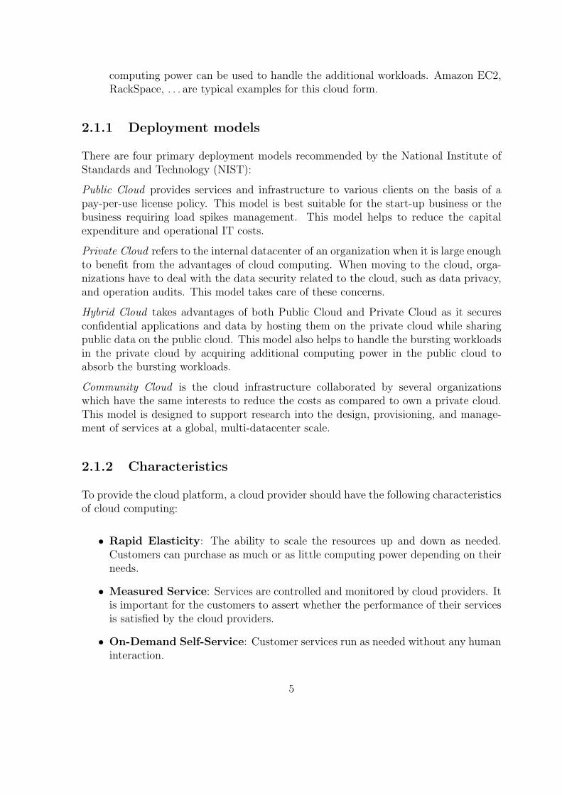
Public Cloud provides services and infrastructure to various clients on the basis of apay-per-use license policy. This model is best suitable for the start-up business or thebusiness requiring load spikes management. This model helps to reduce the capitalexpenditure and operational IT costs.

Private Cloud refers to the internal datacenter of an organization when it is large enoughto benefit from the advantages of cloud computing. When moving to the cloud, orga-nizations have to deal with the data security related to the cloud, such as data privacy,and operation audits. This model takes care of these concerns.

Hybrid Cloud takes advantages of both Public Cloud and Private Cloud as it securesconfidential applications and data by hosting them on the private cloud while sharingpublic data on the public cloud. This model also helps to handle the bursting workloadsin the private cloud by acquiring additional computing power in the public cloud toabsorb the bursting workloads.

Community Cloud is the cloud infrastructure collaborated by several organizationswhich have the same interests to reduce the costs as compared to own a private cloud.This model is designed to support research into the design, provisioning, and manage-ment of services at a global, multi-datacenter scale.

2.1.2 Characteristics

To provide the cloud platform, a cloud provider should have the following characteristicsof cloud computing:

• Rapid Elasticity: The ability to scale the resources up and down as needed.Customers can purchase as much or as little computing power depending on theirneeds.

• Measured Service: Services are controlled and monitored by cloud providers. Itis important for the customers to assert whether the performance of their servicesis satisfied by the cloud providers.

• On-Demand Self-Service: Customer services run as needed without any humaninteraction.

5

• Ubiquitous Network Access: Services can be accessed through standard mech-anisms by both thick and thin clients.

• Resource Pooling Physical and virtual resources are served via multi-tenantmodel. Depending on customer demand, resources are allocated and reallocatedas needed. The customers can also specify the location of resources hosting theirservice through high level abstraction constraints.

Scope of the thesis In this thesis, we focus on IaaS clouds that primarily rely onvirtualization technologies. We develop the high level abstraction of requirements forresource location in public clouds. These requirements provide better Quality of Ser-vices for the cloud-based applications by eliminating the temporary violations that areexplained in the next chapter. As a result, the cloud providers can offer better servicesfor critical applications and cloud infrastructure.

2.2 Virtualization

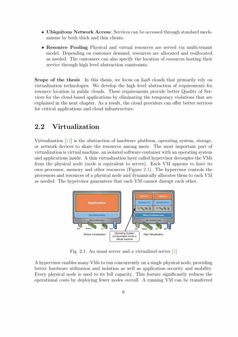
Virtualization [12] is the abstraction of hardware platform, operating system, storage,or network devices to share the resources among users. The most important part ofvirtualization is virtual machine, an isolated software container with an operating systemand applications inside. A thin virtualization layer called hypervisor decouples the VMsfrom the physical node (node is equivalent to server). Each VM appears to have itsown processor, memory and other resources (Figure 2.1). The hypervisor controls theprocessors and resources of a physical node and dynamically allocates them to each VMas needed. The hypervisor guarantees that each VM cannot disrupt each other.

Fig. 2.1: An usual server and a virtualized server [1]

A hypervisor enables many VMs to run concurrently on a single physical node, providingbetter hardware utilization and isolation as well as application security and mobility.Every physical node is used to its full capacity. This feature significantly reduces theoperational costs by deploying fewer nodes overall. A running VM can be transferred

6

from one physical node to another using a process called live migration. Critical appli-cations can be also virtualized [13] to improve performance, reliability, scalability andreduce deployment costs.

Virtualization increases the resource utilization. Most computers do not fully utilizetheir resources which leads to inefficient energy usage [14]. A solution is installing moreapplications on one computer but this way may cause conflicts between the applica-tions. Another possible problem is a single Operating System failure will take downall the applications running in that system [15]. Virtualization is the solution thatallows the applications to run on the same node but isolates them to avoid the con-flicts. Furthermore, virtualization also provides other advantages such as scalability,high availability, fault tolerance, and security which are hardly achieved by traditionalhosting environment.

There are two types of virtualization: bare-metal and hosted. A Bare-metal hypervisormeans the hypervisor is installed directly onto the server hardware without the need fora pre-installed OS on the server. XEN [3], VMware ESXi [16], Citrix XenServer [17]and Microsoft Hyper-V [18] are examples of bare-metal hypervisors. On the other hand,a Hosted hypervisor means the hypervisor is installed as a usual application in the Op-erating System installed on a server. Hosted hypervisors include VMware Workstation,Fusion, VMware Player, VMware Server. Microsoft Virtual PC, Microsoft Server, andSun’s VirtualBox [19]. Bare-metal hypervisors installed right on the server hardwareand therefore offer higher performance and support more VMs per physical CPU thanhosted hypervisors [20].

Live migration [21] is a technique to move a running VM from one physical node toanother with minimal service downtimes. Live migration is performed by taking asnapshot of the VM and coping its memory states from one physical node to another.Then the VM on the original node is stopped after the copy version has run successfullyon the new node.

There are many ways for moving the content of the VM memory from one node toanother. However, migrating a VM requires the balance of minimizing both downtimeand total migration time. The former is the unavailable duration of the service becausethere is no currently executing instance of the VM. The latter is the duration betweenthe start moment of migration and the moment of the origin VM being discarded.

To ensure the consistency of the VM during the migration, the migration process isviewed as a transaction between two involved nodes. A target node which satisfies theresources requirement is selected. A VM is requested on the target node and if thisfails, the origin VM continues running unaffectedly. All data are transferred from theorigin node to the target node. Then the origin VM is suspended and its CPU stateis transferred to the target node. After the target VM is in consistent state, the originVM can be discarded on the origin node to release the resources.

Migrating VMs [21] across distinct physical nodes is a useful tool for datacenter admin-istration. It facilitates fault management, load balancing, and system maintenance in

7

datacenters without or minor disrupting application performance.

2.3 Virtualized Datacenter

A virtualized Datacenter is a pool of cloud infrastructure resources designed specificallyfor enterprise business needs. Those resources include compute, memory, storage andbandwidth. They are made available for cloud customers to deploy and run arbitrarysoftware which can include Operating Systems and applications.

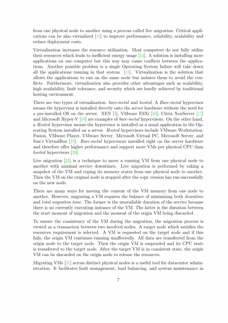
A virtualized datacenter consists of hosting nodes (servers) providing the resources andapplications embedded in VMs consuming the resources. Nodes in a rack connect tothe top-of-rack switch which connects to the upper level switches or routers. Figure 2.2depicts a small virtualized datacenter which consists of three racks. VMs are deliveredto employees through the central VM manager. The virtualized datacenter is dividedinto there zones and each zone can host only the VMs that delivered to the employeesbelonging to that zone. For instance, the VM of a finance staff can only be hosted inFinance Zone for security concerns.

Fig. 2.2: A virtualized datacenter with there server racks[2]

Customers pay for using computing resources of cloud providers and usually they re-quire specific QoS to be maintained by the providers in order to meet their objectives

8

and sustain their operations. The performance metric and other restrictions related tosecurity and availability of an application are formulated in a service level agreement.

2.3.1 SLA to VM Placement Constraint

A service-level agreement (SLA) is a contract between a service provider and a customerthat specifies which services the provider will furnish and the penalties in case of violat-ing the customer expectations. Many service providers provide their customers a SLAso that services of their customers can be measured, justified, and perhaps comparedwith those of outsourcing providers. Cloud providers need to consider and meet differentQoS parameters of each individual customer as negotiated in the specific SLA. Usually,a SLA is expressed in a VM placement constraint.

A VM placement constraint [22] restricts the placement of a VM or a set of VMs. Thetypical VM placement constraint ensures sum of the demands in terms of CPU, memoryand slots of the VMs placed on a certain node does not exceed the node’s capacities inthese resources.

Other VM placement constraints include location and collocation rules [23]. The loca-tion and anti-location constraints restrict or disallow a VM to place on a certain node,respectively. The collocation and anti-collocation constraints are used to place someVMs on the same node, or to place them on distinct nodes. Other advanced constraintscan maximize the load balancing between nodes [24, 25] or minimize the energy cost forhosting VMs in datacenters [4, 26].

Traditional resource management is no longer provide incentives for cloud providersto share their resources with regards to all service requests. A QoS-based resourceallocation mechanism is necessary to regulate the supply and demand of cloud resourcesfor both cloud customers and providers. In virtualized datacenters, VM placementalgorithms are used to regulate the resource allocation.

2.3.2 VM Placement Algorithm

A placement algorithm is the datacenter’s intelligence used to allocate the resources tothe applications in the way that satisfies application requirements simultaneously. Theplacement algorithms are used to improved the scalability [27, 28], performance [29, 30],and reliability [31, 7] of the applications by automatic computing and migrating the VMsdue to network affinity, workload variation, and system maintenance. The placementalgorithms find the placement for each VM to satisfy simultaneously the applicationrequirements and the datacenter objective such as load balancing or energy saving. Thecommon technique is finding a configuration that maps the VMs on the minimum ofnodes and migrating the VMs across the network to reach the found configuration.

9

The problem of placing N VMs on M nodes is often modeled as a vector-packingproblem, assuming that the resource demands remain stable during the re-arrangementof VMs [25]. The physical nodes are modeled as one or more dimensions bins and theVMs are the items with the same number of dimensions to be put into these bins. Inorder to find the optimized mapping, a complete search by enumerating all the possiblecombinations is needed and the complexity becomes NP-hard. To solve this problem,heuristic solutions have been proposed such as algorithms derived from vector-packingalgorithms [32, 31, 26]. There are two types of VM placement algorithm including staticand dynamic VM placement algorithm.

Static VM Placement Algorithm

A static VM placement algorithm is used to optimize the initial resource allocation forworkloads through a configuration to improve application performance, reduce the costsof infrastructure and increase the scalability of datacenters [33, 27, 34]. The configura-tion is not recomputed for a long time until the datacenter administrator re-runs thealgorithm. This strategy leaves many physical servers running at a low utilization formost of the time [14].

Meng et al. [27] design the two-tier approximate algorithm that deploy VMs in largescale datacenters. Chaisiri et al. [33] consider the deployment cost of applications onmulti-datacenters environment. Xu et al. [34] expand the two-level control managementin which local controllers determine the application resource demands and a global con-troller determines the VM placement and resource allocation to minimize the powerconsumption while maintaining the application performance. These algorithms is miss-ing the ability of recomputing the VM placement at runtime when applications varytheir loads or in the event of network and server failures.

Dynamic VM Placement Algorithm

Because of the limitation of static placement algorithms, dynamic placement algorithmsare used to deploy the new VMs in a datacenter and computes a new mapping in theevent of variation of workloads, datacenter maintenance or efficient energy consolida-tion. Dynamic placement algorithms recompute the datacenter configuration in shortertimescales, preferably shorter than the major variation of application workloads. Thehistorical resource utilization and application requirements are used as the input to thealgorithms that deploy VMs in datacenters. Dynamic placement algorithms leveragethe live migration ability.

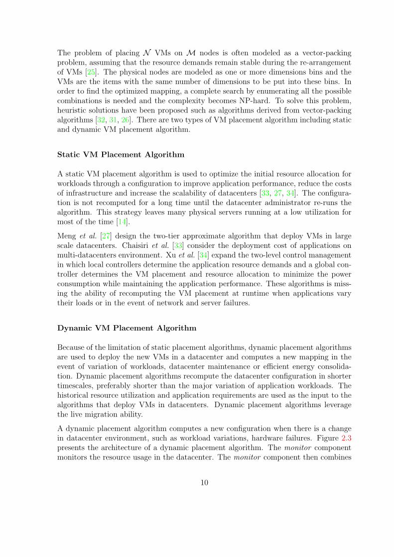
A dynamic placement algorithm computes a new configuration when there is a changein datacenter environment, such as workload variations, hardware failures. Figure 2.3presents the architecture of a dynamic placement algorithm. The monitor componentmonitors the resource usage in the datacenter. The monitor component then combines

10

Datacenter

VMM

VM

1

N1

VMM

VM

m

Nn

VMM

VM

2

N2

VM

m+

1

...

Monitor

resources usage

Dynamic

Algorithm

reconfiguration

Fig. 2.3: dynamic VM placement Algorithm

the resource usage with the application and datacenter constraints to input into thedynamic placement algorithm component. The dynamic placement algorithm computesa reconfiguration plan to transfer the datacenter from current configuration to the newconfiguration. Actions in the reconfiguration plan are scheduled for execution to satisfyVM placement constraints such as maximum capacity or anti-collocation constraint.

Entropy [4] and Wood et al. [35] consider the action schedule in their placement algo-rithms. They justify the need to solve dependencies between migrations. Their adhocheuristics to treat the action scheduling disallow however the addition of any placementconstraints. Bin et al. [36] provide the k-resilient property for a VM in case of serverfailures. The algorithm provides a continuous high-availability by scheduling to migrateonly the VMs marked as highly-available. This approach disallows temporary violationsbut limits the management capabilities of the VMs to this particular use case.

Authors in [29, 7, 5] propose algorithms that support an extensible set of placementconstraints. They however rely on a discrete approach to compute the placement. In [7,5], a node is chosen for every VM randomly. The choice must satisfy the constraintsonce the reconfiguration completed but it is still possible to make two VMs involved inan anti-collocation constraint overlap (see Figure 1.1). Breigand et al. [29] use a scorefunction to choose the best node for each VM. The same temporary overlap may thenappear if putting the first VM on the node hosting the second one leads to a betterscore.

Entropy [4] and BtrPlace [7] (successor to Entropy) are resource managers based onConstraint Programming. They performs dynamic consolidation to put VMs on a re-duced set of nodes. Entropy and BtrPlace use Choco [37], an open-source constraintsolver, to solve a Constraint Satisfaction Problem where the goal is minimizing the num-ber of the running nodes and minimizing migration costs. Furthermore, BtrPlace canbe dynamically configured with placement constraints to provide the Quality of Servicefor applications in a datacenter.

11

2.3.3 Current Btrplace

BtrPlace is a configurable and extensible consolidation manager based on constraintprogramming. BtrPlace provides a high-level scripting language to describe applicationand datacenter requirements. It provides an API to develop and integrate new place-ment constraints. BtrPlace is scalable since it exploits possible partitions implied byplacement constraints, which allows solving sub-problems independently.

Constraint Programming

Constraint Programming (CP) [38] is used to model and solve combinatorial problemsby stating the constraints on the feasible solutions for a set of variables. The solvingalgorithm of CP is independent of the constraints composing the problem and the orderin which they are provided. A problem is modeled as a Constraint Satisfaction Problem(CSP) which consists of a set of variables, a set of domains, and a set of constraints.A domain is the possible values of a variable and a constraint represents the requiredrelations between the values of the variables. A solution of a CSP is an assignment ofa value to each of the variables that satisfies all the constraints simultaneously. Theprimary benefit of CP is the ability to find the global optimum solution. However, in thedynamic VM placement problem, it is more important to provide an optimized solutionin a limited time frame.

BtrPlace allows the data center and application administrator to define their con-straints independently. In this section, we briefly introduce the BtrPlace architecture.Then we describe how BtrPlace models a Reconfiguration Problem.

Architecture

BtrPlace abstracts a datacenter infrastructure in a Model including nodes, VMs, re-source capacity of nodes, resource demand of VMs, state of nodes and VMs. Theexpectation of datacenter and application administrators are expressed in placementconstraints. The model and constraints are inputted in the reconfiguration problemwhich produces a reconfiguration plan to transform the datacenter to the new viableconfiguration.

Reconfiguration Problem

A Reconfiguration Problem (RP) is the problem of finding a viable configuration thatsatisfies all the placement constraints and a reconfiguration plan to transform currentconfiguration into the computed one. A reconfiguration plan consists of a series ofaction that related to VMs and node management such as migrating VM, turning-off

12

or booting VM or node. The actions are scheduled based on their duration to ensuretheir feasibility. For instance, a migration action is feasible if the target node in thedestination configuration has sufficient amount of CPU and memory during and afterthe reconfiguration. Besides satisfying all placement constraints, a reconfiguration planmay have to satisfy with the time constraints.

Variable related to Mappingvhi current host of VM ivqi state of VM inqj state of node j

nvmj the number of VMs hosted by node j

Variable related to ShareableResourcevri amount of resources allocated to VM inrj resource capacity of node j

Variable related to action Managementasi , a

ei moments action i starts and ends, respectively

adi execution duration of action i

Table 2.1: Variables exposed by Reconfiguration Problem

Modeling a Reconfiguration Problem Using CP, a reconfiguration problem isdefined in BtrPlace includes: a model and a set of constraints. The set of nodes N andthe set of virtual machines V are included in the reconfiguration problem. The set ofvariables exposed by a RP is summarized in Table 2.1. Developers use these variablesets to implement new placement constraints.

A model consists of Element, Attributes, Mapping and View. An element is a VM or aphysical node which has several optional attributes. A Mapping indicates the state ofVMs and nodes as well as the placement of the VMs on the nodes. In a Mapping, anode nj is represented by its state nq

j that is either 1 if the node is online or 0 otherwise.

The variable vhi = j indicates the VM vi is running on the node nj. For each dimensionof resources, a View instance provides a domain-specific information of a model. Forexample, The ShareableResource is a View that defined the resource capacity of nodesand resource demand of VMs. A node nj provides an amount of resources of nr

j . A VMvi is considered to consume a fixed amount of resources vri . In addition, the variablesrelated to action management including as, ae denoting the start and the end momentof an action respectively. ad denotes the duration of the action.

Beside the variables exposed in RP, developers can introduce additional variables asneeded. To support for the reconfiguration algorithm, a slice notation is introducedin BtrPlace (Figure 2.4). A slice is a finite period indicates a VM is running on anode and consuming the node’s resource. The height of a slice equals the amount of

13

N1

N2

VM1

VM1

ce

dsde

cs

time

Fig. 2.4: c-slice and d-slice of a VM migrating from N1 to N2

consumed resources. There are consuming slice and demanding slice for a VM involvedin a reconfiguration problem. A consuming slice (c-slice) ci ∈ C of a VM vi is the periodwhich starts at the beginning of the reconfiguration process and terminates at the end ofthe VM migration action. Similarly, a demanding slice (d-slice) starts at the beginningof the VM migration action and terminates at the end of reconfiguration process.

BtrPlace provides the set of placement constraints related to resource management,isolation, fault tolerance, and server management. The set of constraints include the(anti-)affinity rules in VMware DRS [23] and the VM placement features available inAmazon EC2 [39]: availability-zones and dedicated instances. However, the currentimplementation of the constraints focuses on discrete approach which restricts only thefinal placement of the VMs. It can cause the temporary violations of the constraints.

In this thesis, using BtrPlace library I demonstrate the temporary violations of theplacement constraints during reconfiguration of datacenters and provide a solution toprevent these violations.

14

Chapter 3

Reliability of Discrete Constraints

Many computing service providers are deploying datacenters to deliver Cloud computingservices to customers with particular Quality of Services requirements. These require-ments are often translated into placement constraints for dynamic provisioning. Most ofdynamic placement algorithms rely on the discrete constraints [4, 35, 29, 7, 5]. However,this approach may cause the temporary violations of the QoS during the reconfigura-tion. This chapter presents the discrete placement constraints and the evaluation oftheir reliability during the datacenter reconfiguration. The first part presents the defi-nition, practical interest and model of the discrete placement constraints. The seconddemonstrates the evaluation method, and the temporary violations of discrete placementconstraints. We rely on BtrPlace to provide the implementation of discrete constraintsand to exhibit the temporary violations that are allowed by the use of discrete con-straints.

3.1 Discrete constraints

A discrete constraint is a VM placement constraint that imposes the satisfaction ofthe constraint only on the destination configuration. The discrete constraint ensuresthe viability of the destination configuration when the constraint is not satisfied in thecurrent configuration.

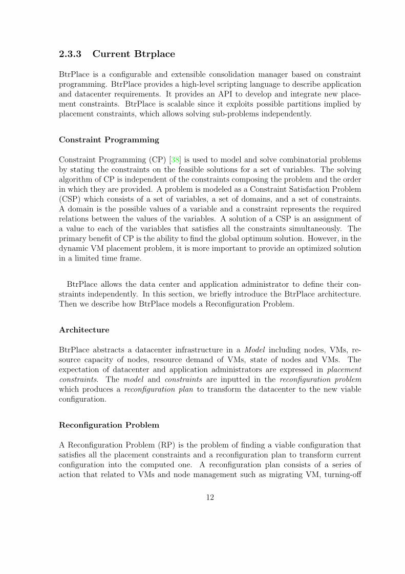
BtrPlace provides many placement constraints covering in isolation, high availability,and high performance. We select some constraints that commonly exists in practiceto evaluate their reliability during the reconfiguration, including spread (anti-affinityVM-VM DRS [23]), among (VM-Host affinity DRS), splitAmong (Availability ZonesEC2 [39]), SingleResourceCapacity, and MaxOnlines. In the next subsection, we presentthe definition, practical interest of these constraints.

spread(M)

The spread constraint keeps the given VMs on distinct nodes in the destination recon-figuration. An example of a spread constraint spread(vm1,vm2) that separates VM1and VM2 is shown in figure 3.1(a). In the destination configuration, this constraint is

15

satisfied as VM1 residing in N1 and VM2 residing in N2. An application administra-tor may use a spread constraint to provide the fault tolerance for his application. Byspreading replicas, the application will be available as long as one replica is still alive.

dhi 6= dhj ∀vi, vj ∈ M, i 6= j (3.1)

In equation (3.1), for the VMs in set M (M ⊂ V), the destination placement of eachVM has to be different from each other.

N1

N2

VM1

VM1

time

VM2

N3 VM3

VM3

(a) spread & among

N1

N2

VM1

time

VM2

N3 VM3

VM3

VM2

(b) splitAmong & maxOnlines

Fig. 3.1: Examples of spread, among, SplitAmong and maxOnlines constraints

among(M, G)

The among constraint limits the placement of the given VMs on a set of nodes amongthe given sets G. In figure 3.1(a), the among constraint among({vm1,vm3},{{N1,N3},N2}} keeps VM1 and VM3 on either set {N1,N3} or N2. Because VM1 and VM3must be in the same set, VM1 is scheduled to move in N1, then VM3 is also migratedto N3. Datacenter and application administrators can use among constraints to grouprelated VMs with regards to specific criteria. For example, the application having highcommunication between VMs may require to host its VMs on a set of nodes that connectto the same edge switch.

dhi ∈ X =⇒ dhj ∈ X ∀i, j ∈ M, i 6= j, ∀X ∈ G (3.2)

In equation (3.2), if the host of VMi belongs to the set X, (X ∈ G), then all the VMsin the set M are required to place in the hosts belonging to the set X.

splitAmong(H,G)

The splitAmong constraint restricts several set of VMs on distinct partitions of nodes.In figure 3.1(b), the constraint splitAmong({{vm1,vm3},vm2}, {{N1,N3},N2}) is used

16

to separate the set {VM1, VM3} from VM2. VM1 and VM2 are co-located at thebeginning, then one of them must be migrated to another node. VM2 is scheduled tomigrate to N2. Furthermore, N3 must be shutdown for energy efficiency, VM3 cannotmigrate to N2 because VM3 and VM2 have to be on different set. Then VM3 is scheduledfor migrating to N1. In the end, different sets of VMs are on distinct partitions of nodes,then the constraint is satisfied. The splitAmong constraint can provide the disasterrecovery property for applications. An application may have multiple replicas and eachreplica is hosted in a distinct zone of the datacenter. In case of disasters, the applicationstill runs without any downtime period.

H is sets of VMs and G is a partitions of nodes. For all VMi and VMj in the same set(∀i, j ∈ A), VMi and VMk in different sets (∀i ∈ A ∧ k ∈ B,A ∩ B = ∅), A,B ∈ H, wehave:

dhi ∈ X =⇒ (dhj ∈ X ∧ dhk /∈ X), X ∈ G (3.3)

In equation (3.3), when a VMi is place on a node belonging to the set X, then the otherVMs are in the same set with VMi have to place on the nodes in the set X and theVMs are not in the same set with VMi must not place on the nodes in the set X.

SingleResourceCapacity(S, r,K)

The SingleResourceCapacity constraint limits the number of resources for VM pro-vision of each node in a set of nodes. The practice interest of this constraint is toreserve resources for the hypervisor management run on each node to guarantee theperformance of the hypervisor.

nrj −

∑

d∈Ddhi=j

dri ≤ K ∀nj ∈ N , j ∈ S (3.4)

In equation (3.4), The resource r of each node in the set S is required to leave some idleresources and this amount is equals to the specified number K.

maxOnlines(S, K)

the maxOnlines constraint restricts the number of online nodes simultaneously. Anexample of maxOnlines constraint is applied in the configuration in the example 3.1(b).maxOnlines({N1,N2,N3},2) allows only 2 nodes to be online at the same time, then N3is selected to go offline to satisfy the constraint. The practical interest of maxOnlinesconstraint is the license restriction or the limitation on capacity of power or coolingsystem. Datacenter administrator has to limit the number of online nodes in the data-center to satisfy the license or to prevent the overload of power or cooling systems. A

17

discrete maxOnlines constraint is modeled as the cardinality of online nodes has to beless than the number that specified in the constraint.

card(nqj = 1) ≤ K, ∀nj ∈ N , j ∈ S (3.5)

In equation (3.5), the state of a node nqj equals to 1 means the node is online. Then the

cardinality of the online nodes in the set of nodes S must be less than or equals to thespecified number K.

3.2 Evaluation Results

We evaluate here the reliability of discrete constraints presented in the previous section.We simulate a datacenter subject to common reconfiguration scenarios and inspect thecomputed reconfiguration plans to detect temporary violations.

3.2.1 Simulation Setup

We describe the datacenter setup, applications with Service Level Agreement (SLA) andthe reconfiguration scenarios that existed in real datancenters.

Datacenter

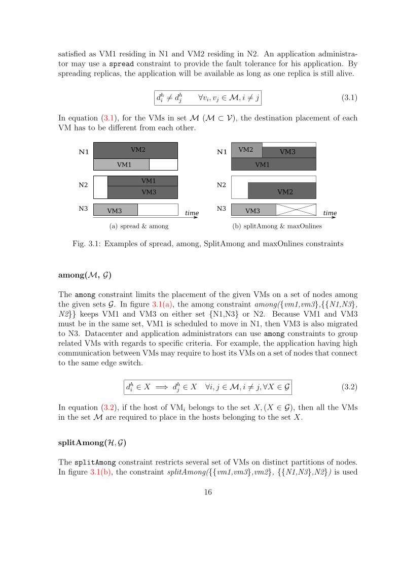
The simulated datacenter consists of 256 nodes split over 2 clusters. Each cluster consistsof 8 racks of 16 nodes each. Inside a rack, nodes are connected through a non-blockingnetwork. Each node has 128 GB RAM and a computational capacity of 64 uCPU, a unitsimilar to ECU in Amazon EC2 [39] to abstract the hardware. We simulate 350 3-tierweb applications, each having a structure generated randomly to use between 6 and 18VMs, with 2 to 6 VMs per tier. At total, the datacenter runs 5,200 VMs. Table 3.1summarizes the VM resource consumption for each tier. VMs in the Tier 1 requirea few and balanced amount of resources. VMs in the Tier 2 and 3 are computationand memory intensive, respectively. By default, each VM consumes only 25% of themaximum allowed. This makes the datacenter uCPU and memory usage equal to 68%and 40% respectively.

SLAs in the datacenter

A SLA is attached to each application. For each tier, one spread constraint requiresdistinct nodes for the VMs to provide fault tolerance. This mimics the VMWare DRSanti-affinity rule. One among constraint forces VMs of the third tier to be hosted on

18

TierInitial consumption Max. consumptionuCPU RAM uCPU RAM

1 1 1 GB 2 4 GB2 4 2 GB 14 7 GB3 1 4 GB 4 17 GB

Table 3.1: VM characteristics

a single rack to benefit from the fast interconnect. Last, 25% of the applications usea splitAmong constraint to separate the replicas among the two clusters. This mimicsAmazon EC2 high-availability through location over multiple availability zones.

The datacenter is also subject to placement constraints. The maximum number of onlinenodes is restricted to 240 by a maxOnlines constraint to simulate a hypervisor-basedlicensing model [17]. The 16 remaining nodes are offline and spread across the racks toprepare for application load spikes or hardware failures. Last, one singleResourceCa-pacity constraint preserves 4 uCPU and 8 GB RAM on each node for the hypervisormanagement operations.

Reconfiguration scenarios

On the simulated datacenter, we consider four reconfiguration scenarios that mimicindustrial use cases[40]:

Vertical Elasticity. In this scenario, applications require more resources for theirVMs to support an increasing workload. In practice, 10% of the applications require anamount of resources equals to the maximum allowed. With BtrPlace, this is expressedusing preserve constraints to ask for resources.

Horizontal Elasticity. In this scenario, applications require more VMs to supportan increasing workload. In practice, 25% of the applications double the size of theirtiers. With BtrPlace, this is expressed using running constraints to ask to run moreVMs.

Hardware Failure. Google reports that yearly, a network outage makes 5% of theservers instantly unreachable. [41] This scenario is simulated by setting randomly 5% ofthe nodes in a failure state and asking to restart their VMs on other nodes.

Boot Storm. In virtual desktop infrastructures, numerous desktop VMs are startedsimultaneously before the working hours. To simulate this scenario, 400 new VMs arerequired to boot. Their characteristics are chosen randomly among those described inTable 3.1 and their resource consumption is set to the maximum allowed.

19

3.2.2 Evaluating Temporary Violations

For each scenario, we generate 100 different instances that satisfy the placement con-straints. The simulator runs on a dual CPU Xeon at 2.27 GHz having 24 GB RAM thatruns Fedora 18 and OpenJDK 7.

Temporary violated SLAs

ScenarioViolated ActionsSLAs VM Boot Migrate Node Boot

Vertical Elasticity 41.74 0% 100% 0%Horiz. Elasticity 0.54 99% 1% 0%Server Failure 31 62% 35% 3%Boot Storm 1.37 95% 5% 0%

Table 3.2: Violated SLAs and actions composing the reconfiguration plans.

A SLA is failed when at least one among its constraints is violated. Table 3.2 sum-marizes the number of SLA failures and the distribution of the actions that composesthe reconfiguration plans. We observe that the Vertical Elasticity and the ServerFailure scenarios lead to the most violations. Furthermore, we observe a relation be-tween the number of migrations and the number of SLA violations. Initially, the currentplacement of the running VMs satisfies the constraints. During a reconfiguration, someVMs are migrated to their new hosts and once all the migrations are terminated, theresulting placement also satisfies the constraints. Until the reconfiguration is complete,a part of the VMs may be on their new hosts while the others are still waiting for be-ing migrated. This leads to an unanticipated combination of placements that was notunder the control of the constraints. This explanation is also valid for constraints thatmanage the node state, such as maxOnlines. When the reconfiguration plan consistsof booting VMs only, this situation cannot occur with the studied set of constraints.The placement constraints ignore non-running VMs and as each VM is deployed on asatisfying host, temporary violation is not possible.

Distribution of the violated constraints

Figure 3.2 presents the average distribution of violated constraints in violated SLAsusing box-and-whisker plots. The top and the bottom of each box denote the firstand the third quartiles, respectively. The notch around a median indicates the 95%confidence interval. We observe among is the most violated constraint. Furthermore,with a distribution that exceeds 100%, multiple constraints can be violated within asingle SLA. The violations are explained by the behavior of BtrPlace. To compute smallreconfiguration plans, BtrPlace tries to keep each VM on its current node, otherwise, itchooses a new satisfying host randomly. If a VM involved in an among constraint must

20

●

●●

●●●●●

●

●●●

●

●

●

●●

●●

●

●

0

25

50

75

100

VerticalElasticity

HorizontalElasticity

ServerFailure

BootStorm

viol

atio

ns

spread among splitAmong maxOnlines

Fig. 3.2: Distribution of the violated constraints

be migrated, BtrPlace has 94% chances to select a node on another rack, hence violatingthe constraint until the other involved VMs are relocated to this rack. This violationmay reduce the performance of the application due to the slow interconnect between theVMs. For a VM subjects to a spread constraint, there is 2% chances at worst to selecta node that already hosts a VM involved in the same constraint. The constraint willthen be violated, leading to a potential single point of failure, until the other VM hasbeen relocated elsewhere. For a VM subjects to a splitAmong constraint, the chances toselect a node in the other cluster are 50% and the consequences of the resulting violationare similar to spread. Figure 3.2 reports more violation of spread than splitAmong

constraints. There are 14 times more spread constraints so the chances to violate atleast one constraint are higher.

The maxOnlines constraint has been violated 5 times, all in the vertical elasticity

scenario. In these cases, the load increase saturated some racks. BtrPlace chose to bootthe rack’ spare node to absorb the load and to shutdown a node in a non-saturatedrack in exchange to satisfy the constraint at the end of the reconfiguration. BtrPlaceschedules the actions as soon as possible. It then decided to boot the spare node beforeshutting down the other node which lead to a temporary violation of the constraint.With floating hypervisor licenses, this would lead to a non-applicable reconfigurationplan. The singleResourceCapacity constraint was never violated: BtrPlace schedulesthe VM migrations before increasing their resource allocation, it is then not possible tohave a resource consumption that exceeds the host capacity.

Conclusion on discrete constraints

This experiment reveals temporary violations occur in BtrPlace despite the usage ofplacement constraints. We also discussed in Chapter 2 that other placement algo-rithms [29, 5] may also compute plans leading to temporary violations. Their causeis only related to the lack of controls over the computation of the actions schedule.

21

The consequences of these violations depend on the application requirements. For theapplications that require high availability, the temporary violation of spread and spli-

tAmong constraints can lead to the unavailable of services in case the VMs co-allocate inthe same node and the node fails. The applications that require high performance mayexperience degradation in performance if the VMs involved in the among constraint arenot co-allocated. Similarly, the node performance may have bottlenecks if the hypervi-sors do not have enough resources. Finally, meeting license restriction is important forthe datacenter as every single license violation costs an amount of money.

In the next chapter, we present continuous constraints that help to prevent the tempo-rary violations during the reconfiguration. The continuous constraints control not onlythe placement of VMs but also the action schedule.

22

Chapter 4

Elimination of TemporaryViolations with ContinuousConstraints

Depending on the users expectations, they may require the permanent satisfaction ofthe application requirements. In this chapter, we propose continuous constraints to con-trol the VM placement and action schedule guaranteeing the satisfaction of constraintscontinuously. We discuss the implementation and evaluation of continuous constraintswhose discrete correspondences are previously evaluated in section 3.2.

4.1 Continuous constraint

A continuous constraint is a VM placement constraint that imposes the satisfactionof the constraint not only on the destination configuration but also during the recon-figuration. Continuous constraints can be used for critical application and datacenterrequirements to ensure their satisfaction at any moment of the reconfiguration.

The implementation of continuous constraints requires a new look on the restrictionsto express. To implement a discrete constraint, a developer only pays attention to thefuture placement of the VMs and the next state of the nodes. To implement continuousconstraints, he also has to integrate the schedule of the associated actions. A pureplacement problem in discrete constraints becomes a scheduling problem that is harderto tackle in continuous constraints.

BtrPlace already exposes not only variables related to the VM placement and nodestate at the end of the reconfiguration, but also variables related to the action schedule.We have implemented the continuous constraints by extending the discrete ones to act,when necessary, on the action schedule.

23

4.2 Modeling the continuous constraints

Different constraints have different level of difficulty. Some constraints, like among andsplitAmong, do not require the action schedule to implement their continuous restric-tion. Other constraints need to take into consider the order of actions’ execution toachieve the continuous satisfaction.

The continuous implementation of among and splitAmong does not need to manipulatethe action schedule. If a VM is already running on a node, the continuous implementa-tion just restricts the VM placement to the associated group.

The continuous implementation of spread prevents the VMs from overlapping. Inpractice, when a VM is migrated to a node hosting another VM involved in the sameconstraint, we force the start time of the migration action to be greater or equal to thevariable denoting the moment the other VM will leave the node.

Other constraints are much more complex than the implementation of spread con-straints which simply restricts the start and the end moments of migrations. In thenext subsections, we compare the discrete and continuous restriction of the constraintsthat I have developed in the thesis.

4.2.1 MaxOnlines

The definition and practical interest of MaxOnlines constraint are presented in sec-tion 3.1.

Discrete restriction The discrete implementation of maxOnlines extracts the booleanvariables that indicate if the nodes must be online at the end of the reconfiguration andforces their sum to be at most equal to the given amount (4.1).

card(nqj = 1) ≤ K, ∀nj ∈ N , j ∈ S (4.1)

Continuous restriction For a continuous implementation, we model the online pe-riods of the nodes and guarantee that their overlapping never exceeds the limit K.Because BtrPlace does not provide variables to model the online period of a node, wehave then defined this period from pre-existing variables related to the scheduling of thepotential node action.

We defined psi and pei in equation (4.2) as the moments a node i becomes online oroffline, respectively. These two variables are declared in the Power-Time View and areinjected in the Reconfiguration Problem. If the node is already online, figure 4.1(a), psiequals the reconfiguration start and pei equals to the sum of the hosting end momenthe of node i and the duration ad of the shutdown action. In case of the node staying

24

S

psas aepehe rpe

psasae pe herpe

ad

time

(a) Shutdownable action

psas ae peherpe

psasae pehe rpe

ad

B

time

(b) Bootable action

Fig. 4.1: Modeling Power-Start and Power-End of a node

online, the shutdown action is not executed and the variables as, ad, ae all equal to 0. Asa result, psi equals 0, and pei equals h

e, equivalent to rpe, the end of the reconfiguration.Otherwise, if the node is offline at first, figure 4.1(b), psi equals the action start and peiequals the hosting end moment he of node i. In case of the node staying offline duringthe reconfiguration, the boot action is not executed, and as a consequence, psi and peiare equal to 0. The online period for the node i is then defined with a time intervalbounded by psi and pei . We finally restrict the overlap of the online periods as follow:

N1

N2 N3

time

N1

N2

N3

S

B

ps pe rpe2 2

ps3

pe3

pe1ps

1

Fig. 4.2: Cumulative scheduling of maxOnlines constraint

card({i|psi ≤ t ≤ pei}) ≤ K, ∀t ∈ T (4.2)

This restriction can be implemented as a cumulative constraint[42], available in Choco [37],the CP solver used in BtrPlace. Cumulative is a common scheduling constraint thatrestricts the overlapping of tasks that have to be executed on a resource. Figure 4.2depicts a cumulative scheduling of a maxOnlines constraint which only allows 2 nodesonline simultaneously.

25

4.2.2 MinSpareNode(S, K) & MaxSpareNode(S, K)

MinSpareNode and MaxSpareNode manage the maximum and minimum number of sparenodes in the node set S (S ⊂ N ), respectively. A spare node is a node is online andidle (do not host any VM) to be available for VM provision when there is a load peak.A node provides the resources as coarse-grain, so it is easier to control the resources atthe node level. The practical interest of minSpareNode is reserving a specific number ofspare nodes to deal with application load spike whist the practical of maxSpareNode isrestricting the number of spare nodes to use the power efficiently.

card({nqj = 1 ∧ nvm

j = 0}) ≥ K, ∀nj ∈ S (4.3)

Discrete restriction In equation (4.3), a spare node is modeled as a node is beingonline and not hosting any VM. For minSpareNode constraints, the cardinality of thespare nodes in the set S has to be greater or equals to the constant number K indicatedin the constraint. In the opposite, this number has to be less than or equals to K inmaxSpareNode constraints.

ie

time

VM1

VM2

VM1

VM2

ieis

is rpe

B

N1

N2

Fig. 4.3: Modeling idle period of a node

continuous restriction Similar to the online period of a node, the idle period is notdefined yet in BtrPlace. A node is in the spare period if it is online and does not host anyVM. We define idle-start and idle-end (is and ie in figure 4.3) to indicate the momentof the node becomes idle and occupied, respectively. If the node is already online, theidle-start equals to the moment of the c-slice that leaves the node last. On the otherhand, if the node is offline at the beginning, the idle-start equals to the hosting-start ofthe node. The idle-end of the node equals to the moment of the d-slice that arrives thenode first. If no VM arrives on the node, the idle-end equals to the hosting-end of thatnode. The idle period of a node then equals to the period between the idle-start andidle-end.

26

idle-starti =

{

MAX(ce) if nqi = 1,

hs if nqi = 0.

(4.4)

idle-endi =

{

MIN(ds) if nqi = 1,

he if nqi = 0.

(4.5)

MinSN : K ≤ card({i|idle-starti ≤ t ≤ idle-endi}) ≤ N , ∀t ∈ T (4.6)

MaxSN : 0 ≤ card({i|idle-starti ≤ t ≤ idle-endi}) ≤ K, ∀t ∈ T (4.7)

The Cumulative constraint is used to prevent the limit of the number of spare nodesduring the reconfiguration. The node idle-start is identical to the the task start. Anode idle period is identical to the task duration. The limitation is the capacity ofthe resources. The Cumulative constraint has a variable of minimum consumption ofresources. In this model, the minimum consumption variable is identical to the minimumof idle nodes. Then for MinSpareNode constraint, we set the minimum consumptionvariable to the numberK and the capacity variable to the total number of nodes involvedin the constraint. On the other hand, the minimum consumption can be zero, and thecapacity equals to K in MaxSpareNode constraint.

4.2.3 MinSpareResource(S, r, K)

The MinSpareResource constraint reserves at least a specified number K of idle re-sources r directly available for VM provision on the set of node S (S ⊂ N ). Thepractical interest of the constraint is preventing the nodes from saturation whenever aload spike occurs. Turning on a node or migrating a VM out of the saturated nodemay take long time, leading to some certain performance degradation of applications.The MinSpareResource constraint is used in this situation to keep an amount of idleresources to absorb the load spike.

∑

j∈S

nqjn

rj −

∑

dri ≥ K, ∀d ∈ D, dhi = j (4.8)

Discrete restriction The model of MinSpareResource is represented in equation (4.8).The number of spare resources equals to the difference of the capacities to the sum ofallocated resources. The resource r can be CPU, memory, etc. The number of spare re-sources has to be greater or equal to the constant number K indicated in the constraint.

27

∑

j∈S

nqjn

rj −

∑

∀c∈Cchi=j

cri −∑

∀d∈Ddhi=j

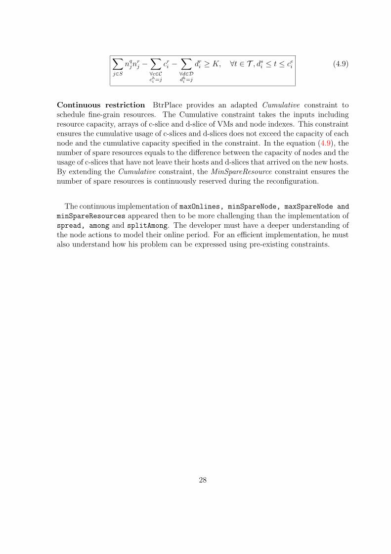
dri ≥ K, ∀t ∈ T , dsi ≤ t ≤ cei (4.9)

Continuous restriction BtrPlace provides an adapted Cumulative constraint toschedule fine-grain resources. The Cumulative constraint takes the inputs includingresource capacity, arrays of c-slice and d-slice of VMs and node indexes. This constraintensures the cumulative usage of c-slices and d-slices does not exceed the capacity of eachnode and the cumulative capacity specified in the constraint. In the equation (4.9), thenumber of spare resources equals to the difference between the capacity of nodes and theusage of c-slices that have not leave their hosts and d-slices that arrived on the new hosts.By extending the Cumulative constraint, the MinSpareResource constraint ensures thenumber of spare resources is continuously reserved during the reconfiguration.

The continuous implementation of maxOnlines, minSpareNode, maxSpareNode and

minSpareResources appeared then to be more challenging than the implementation ofspread, among and splitAmong. The developer must have a deeper understanding ofthe node actions to model their online period. For an efficient implementation, he mustalso understand how his problem can be expressed using pre-existing constraints.

28

4.3 Trade-off between reliability and computability

In this section, we present the preliminary results of the implementation in order toprovide the continuous satisfaction of the constraints. The results show the continu-ous constraints have prevented the temporary violations during the reconfiguration ofdatacenters. Nevertheless, the result also exhibit obstacles of continuous constraints incomputing the viable configuration.

4.3.1 Reliability of continuous constraints

VerticalElasticity

HorizontalElasticity

ServerFailure

BootStorm

Sol

ved

inst

ance

s0

2040

6080

100

Discrete, 1 min.Continuous, 1 min.Discrete, 5 min.Continuous, 5 min.

Fig. 4.4: Solved instances depending on the restriction.

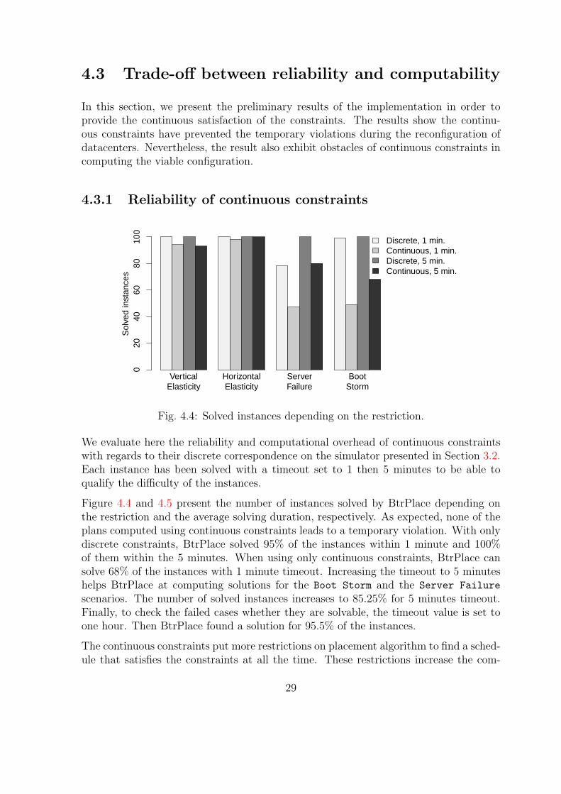
We evaluate here the reliability and computational overhead of continuous constraintswith regards to their discrete correspondence on the simulator presented in Section 3.2.Each instance has been solved with a timeout set to 1 then 5 minutes to be able toqualify the difficulty of the instances.

Figure 4.4 and 4.5 present the number of instances solved by BtrPlace depending onthe restriction and the average solving duration, respectively. As expected, none of theplans computed using continuous constraints leads to a temporary violation. With onlydiscrete constraints, BtrPlace solved 95% of the instances within 1 minute and 100%of them within the 5 minutes. When using only continuous constraints, BtrPlace cansolve 68% of the instances with 1 minute timeout. Increasing the timeout to 5 minuteshelps BtrPlace at computing solutions for the Boot Storm and the Server Failure

scenarios. The number of solved instances increases to 85.25% for 5 minutes timeout.Finally, to check the failed cases whether they are solvable, the timeout value is set toone hour. Then BtrPlace found a solution for 95.5% of the instances.

The continuous constraints put more restrictions on placement algorithm to find a sched-ule that satisfies the constraints at all the time. These restrictions increase the com-

29

plexity of the algorithm to find the solution. Some instances that are higher in initialworkload are more complex to find a solution than the other instances. This circum-stance increases the time for the algorithm to the solution. The more timeout theplacement algorithm has, the more number of instances can be solved.

4.3.2 Computational overheads for continuous constraints

The additional restrictions provided by the continuous constraints may impact the per-formance of the underlying placement algorithm. The overhead of the continuous con-straints is explained by their additional computations to disallow temporary violations.This overhead is acceptable for the Vertical Elasticity and Horizontal Elastic-

ity scenarios with regards to their benefits in terms of reliability as the computationduration in these scenarios just increases a couple of seconds.

VerticalElasticity

HorizontalElasticity

ServerFailure

BootStorm

Sol

ving

dur

atio

n (s

econ

ds)

010

2030

40

Discrete, 1 min.Continuous, 1 min.Discrete, 5 min.Continuous, 5 min.

Fig. 4.5: Solving duration depending on the restriction.

For the Boot Storm and the Server Failure scenarios, the overhead is more important.BtrPlace was not able to solve 30 instances within the allotted 5 minutes. This confirmsthese classes of problems are much more complex to solve. With the timeout set to 5minutes, we observe a high standard deviation. This reveals a few instances are very hardto solve within a reasonable duration. Comparing these hard instances with the othersmay exhibit performance bottlenecks and demand for optimizing the implementation ofcontinuous constraints. We are currently studying the remaining unsolved instances butwe think some of these instances cannot be solved without a relaxation of the continuouscomponent of some constraints.

Although, continuous constraints prevent the temporary violations of SLAs during data-center reconfiguration, they also increase the computational overheads for the placementalgorithm to find a solution. The viable reconfiguration plan sometimes cannot be foundwithin a certain amount of time. Then a possible solution is providing users a tool tocharacterize the constraint tolerance.

30

Chapter 5

Conclusion

Cloud computing offers the opportunities to host applications in virtualized datancentersto reduce the deployment costs for customers and to utilize the hosting infrastructureeffectively. The use of virtualization techniques provides the ability to consolidate severalVMs on the same physical node, to resize a VM resources as needed and to migrate VMacross network for server maintenance. The primary challenge for cloud providers isautomatically managing their datacenters while taking into account customers’ SLAsand resource management costs.

In a virtualized datacenter, customers express their SLAs through placement constraints.A VM placement algorithm is then in charge of placing the VMs on the nodes accordingto the constraints stated in the customer SLAs. Usually, a constraint manages the VMplacement only at the end of the reconfiguration process and ignores the datacenterintermediary states between the beginning and the end of the reconfiguration process.We defined this type of constraints is the discrete placement constraint.

Through simulating datacenter reconfiguration, we showed the discrete constraints arenot sufficient to satisfy the SLAs continuously. The VM placement algorithm does nottake into account of actions schedule and this approach may indeed lead to temporaryviolations. We exhibited these violations through BtrPlace, one of the placement algo-rithms that rely on discrete placement constraints. We observed the violations occurwhen a reconfiguration plan aims at fixing a resource contention of the VMs or resourcefragmentation using migrations without action scheduling.

This thesis addresses the problem of placement algorithms relying discrete constraints.We proposed continuous constraints to satiate the SLA satisfaction by scheduling theactions in the reconfiguration. We modeled and implemented preliminary version ofcontinuous constraints to prevent the temporary violations. The continuous constraintsare evaluated with the same settings of their discrete correspondence. We asserted thecontinuous constraints improve the datacenter reliability by eliminating all observedtemporary violations.

The implementation of the continuous constraints puts more challenges for the devel-opers. It first requires detailed understanding of the principles of a reconfiguration. Italso transforms a supposed placement problem into a scheduling one which is harderto tackle. This means a developer has to study what are provided by the reconfigura-tion and which schedule and new variables he may need to use to achieve the goal of

31

continuous constraints.

Finally, the continuous constraints provide reliability for SLAs, but their computationalcomplexity reduces significantly the scalability of the placement algorithm. Applicationsin load spikes may experience some degradation while the placement algorithm spendsmore time on finding a solution. We need to define the trade-off between reliabilityand performance of application for users to choose. Then the placement algorithmcan enhance the computation by respecting the important constraints and ignoring theconstraints that can stand with some transient failures.

Future Research

We want to investigate on the causes that can lead to temporary violations. Throughobservation, VM migration is the key contributor for these violations. Energy-efficientplacement algorithms rely heavily on VM migrations. These algorithms are widely usedand should be studied as they shall be subject to such violations. We also want toconsider placement constraints that address new concerns, such as services dependencyand automatic balancing, to investigate for their likelihood of being subject to violations,and for the consequences in case of violations.

We observed that continuous constraints impact the performance of a placement algo-rithm, while not being constantly required to deny temporary violations. We want thento explore the situations that make continuous placement constraints unnecessary andrely on a static analysis of the problems to detect these situations.

Finally, we noticed continuous constraints may lead to unsolvable problems. In thissituation, a user may prefer a temporary violation of its SLA. This however implies toallow the users to characterize their tolerance. We want then to model the cost of aconstraint violation and integrate this notion inside BtrPlace.

32

Bibliography

[1] E. Siebert, “What is virtualization.” http://itknowledgeexchange.techtarget.com/virtualization-pro/what-is-virtualization/. Accessed: 2013-08-05.vii, 6

[2] K. Surksum, “A comprehensive framework for securing virtual-ized data center.” http://virtualization.info/en/news/2010/12/

paper-a-comprehensive-framework-for-securing-virtualized-data-center.

html. Accessed: 2013-08-06. vii, 8

[3] P. Barham, B. Dragovic, K. Fraser, S. Hand, T. Harris, A. Ho, R. Neugebauer,I. Pratt, and A. Warfield, “Xen and the art of virtualization,” in 19th SOSP,pp. 164–177, 2003. 1, 7

[4] F. Hermenier, X. Lorca, J.-M. Menaud, G. Muller, and J. Lawall, “Entropy:a consolidation manager for clusters,” in Proceedings of the 2009 ACM SIG-PLAN/SIGOPS international conference on Virtual execution environments, VEE’09, (New York, NY, USA), pp. 41–50, ACM, 2009. 1, 9, 11, 15

[5] K. Tsakalozos, M. Roussopoulos, and A. Delis, “Hint-based execution of workloadsin clouds with nefeli,” Parallel and Distributed Systems, IEEE Transactions on,vol. 24, no. 7, pp. 1331–1340, 2013. 1, 11, 15, 21

[6] T. Wood, P. Shenoy, A. Venkataramani, and M. Yousif, “Black-box and gray-boxstrategies for virtual machine migration,” in Proceedings of the 4th USENIX con-ference on Networked systems design & implementation, NSDI’07, (Berkeley,CA, USA), pp. 17–17, USENIX Association, 2007. 1

[7] F. Hermenier, J. Lawall, and G. Muller, “Btrplace: A flexible consolidation managerfor highly available applications,” IEEE Transactions on Dependable and SecureComputing, vol. 99, no. PrePrints, p. 1, 2013. 1, 9, 11, 15

[8] C. Dupont, T. Schulze, G. Giuliani, A. Somov, and F. Hermenier, “An energy awareframework for virtual machine placement in cloud federated data centres,” in Pro-ceedings of the 3rd International Conference on Future Energy Systems: Where En-ergy, Computing and Communication Meet, e-Energy ’12, (New York, NY, USA),pp. 4:1–4:10, ACM, 2012. 1

[9] G. Jung, M. A. Hiltunen, K. R. Joshi, R. D. Schlichting, and C. Pu, “Mistral:Dynamically managing power, performance, and adaptation cost in cloud infras-

33

tructures,” in Proceedings of the 2010 IEEE 30th International Conference on Dis-tributed Computing Systems, ICDCS ’10, (Washington, DC, USA), pp. 62–73, IEEEComputer Society, 2010. 1

[10] M. Armbrust, A. Fox, R. Griffith, A. D. Joseph, R. Katz, A. Konwinski, G. Lee,D. Patterson, A. Rabkin, I. Stoica, and M. Zaharia, “A view of cloud computing,”Commun. ACM, vol. 53, pp. 50–58, Apr. 2010. 4

[11] B. P. Rimal, E. Choi, and I. Lumb, “A taxonomy and survey of cloud computingsystems,” in INC, IMS and IDC, 2009. NCM’09. Fifth International Joint Confer-ence on, pp. 44–51, Ieee, 2009. 4

[12] G. J. Popek and R. P. Goldberg, “Formal requirements for virtualizable third gen-eration architectures,” Communications of the ACM, vol. 17, no. 7, pp. 412–421,1974. 6

[13] “Virtualizing Business-Critical Applications on VSphere,”tech. rep., VMware, 2012.7

[14] L. A. Barroso and U. Holzle, “The case for energy-proportional computing,”Com-puter, vol. 40, no. 12, pp. 33–37, 2007. 7, 10

[15] D. Meisner, B. T. Gold, and T. F. Wenisch, “Powernap: eliminating server idlepower,” in ACM Sigplan Notices, vol. 44, pp. 205–216, ACM, 2009. 7

[16] C. Chaubal, “The architecture of vmware esxi,”VMware White Paper, 2008. 1, 7

[17] “Citrix store.” http://store.citrix.com. 7, 19

[18] A. Velte and T. Velte, Microsoft virtualization with Hyper-V. McGraw-Hill, Inc.,2009. 1, 7

[19] J. Watson, “Virtualbox: bits and bytes masquerading as machines,”Linux Journal,vol. 2008, no. 166, p. 1, 2008. 7

[20] V. Chaudhary, M. Cha, J. Walters, S. Guercio, and S. Gallo, “A comparison of vir-tualization technologies for hpc,” in Advanced Information Networking and Appli-cations, 2008. AINA 2008. 22nd International Conference on, pp. 861–868, IEEE,2008. 7

[21] C. Clark, K. Fraser, S. Hand, J. G. Hansen, E. Jul, C. Limpach, I. Pratt, andA. Warfield, “Live migration of virtual machines,” in 2nd NSDI, pp. 273–286, 2005.7

[22] C. Hyser, B. Mckee, R. Gardner, and B. J. Watson, “Autonomic virtual machineplacement in the data center,” Hewlett Packard Laboratories, Tech. Rep. HPL-2007-189, pp. 2007–189, 2007. 9

34

[23] D. Epping and F. Denneman, VMware vSphere 4.1 HA and DRS technical deepdive.CreateSpace, 2010. 9, 14, 15

[24] A. Singh, M. Korupolu, and D. Mohapatra, “Server-storage virtualization: integra-tion and load balancing in data centers,” in Proceedings of the 2008 ACM/IEEEconference on Supercomputing, p. 53, IEEE Press, 2008. 9

[25] M. Mishra and A. Sahoo, “On theory of vm placement: Anomalies in existingmethodologies and their mitigation using a novel vector based approach,” in CloudComputing (CLOUD), 2011 IEEE International Conference on, pp. 275–282, IEEE,2011. 9, 10

[26] A. Verma, P. Ahuja, and A. Neogi, “pmapper: power and migration costaware application placement in virtualized systems,” in Proceedings of the 9thACM/IFIP/USENIX International Conference on Middleware, Middleware ’08,(New York, NY, USA), pp. 243–264, Springer-Verlag New York, Inc., 2008. 9,10

[27] X. Meng, V. Pappas, and L. Zhang, “Improving the scalability of data center net-works with traffic-aware virtual machine placement,” in INFOCOM, 2010 Proceed-ings IEEE, pp. 1–9, IEEE, 2010. 9, 10

[28] C. Tang, M. Steinder, M. Spreitzer, and G. Pacifici, “A scalable application place-ment controller for enterprise data centers,” in Proceedings of the 16th internationalconference on World Wide Web, pp. 331–340, ACM, 2007. 9

[29] D. Breitgand, A. Marashini, and J. Tordsson, “Policy-driven service placementoptimization in federated clouds,” IBM Research Division, Tech. Rep, 2011. 9, 11,15, 21

[30] J. Sonnek, J. Greensky, R. Reutiman, and A. Chandra, “Starling: Minimizingcommunication overhead in virtualized computing platforms using decentralizedaffinity-aware migration,” in Parallel Processing (ICPP), 2010 39th InternationalConference on, pp. 228–237, 2010. 9

[31] N. Bobroff, A. Kochut, and K. Beaty, “Dynamic placement of virtual machines formanaging sla violations,” in Integrated Network Management, 2007. IM ’07. 10thIFIP/IEEE International Symposium on, pp. 119–128, 2007. 9, 10

[32] F. Hermenier, S. Demassey, and X. Lorca, “Bin repacking scheduling in virtualizeddatacenters,”Principles and Practice of Constraint Programming–CP 2011, pp. 27–41, 2011. 10

[33] S. Chaisiri, B.-S. Lee, and D. Niyato, “Optimal virtual machine placement acrossmultiple cloud providers,” in Services Computing Conference, 2009. APSCC 2009.IEEE Asia-Pacific, pp. 103–110, IEEE, 2009. 10

35

[34] J. Xu and J. A. Fortes, “Multi-objective virtual machine placement in virtualizeddata center environments,” in Green Computing and Communications (GreenCom),2010 IEEE/ACM Int’l Conference on & Int’l Conference on Cyber, Physical andSocial Computing (CPSCom), pp. 179–188, IEEE, 2010. 10

[35] T. Wood, G. Tarasuk-Levin, P. Shenoy, P. Desnoyers, E. Cecchet, and M. D. Cor-ner, “Memory buddies: exploiting page sharing for smart colocation in virtualizeddata centers,” in Proceedings of the 2009 ACM SIGPLAN/SIGOPS internationalconference on Virtual execution environments, VEE ’09, (New York, NY, USA),pp. 31–40, ACM, 2009. 11, 15

[36] E. Bin, O. Biran, O. Boni, E. Hadad, E. K. Kolodner, Y. Moatti, and D. H. Lorenz,“Guaranteeing high availability goals for virtual machine placement,” 2012 IEEE32nd International Conference on Distributed Computing Systems, vol. 0, pp. 700–709, 2011. 11

[37] “Choco: an open source Java constraint programming library,” Research report10-02-INFO, Mines de Nantes, 2010. 11, 25

[38] P. Shaw, “A constraint for bin packing,” in Principles and Practice of ConstraintProgramming (CP’04), vol. 3258 of Lecture Notes in Computer Science, (Toronto,Canada), pp. 648–662, Springer, 2004. 12

[39] “Amazon EC2.” http://aws.amazon.com/ec2/. 14, 15, 18

[40] V. Soundararajan and J. M. Anderson, “The impact of management operations onthe virtualized datacenter,”SIGARCH Comput. Archit. News, vol. 38, pp. 326–337,June 2010. 19

[41] Dean, Jeff, “Designs, lessons and advice from building large distributed systems,”in Keynote of the International Conference on Large-Scale Distributed Systems andMiddleware Conference, 2009. 19

[42] Y. Caseau and F. Laburthe, “Cumulative scheduling with task intervals.,” in Pro-ceedings of the 1996 Joint International Conference and Symposium on Logic Pro-gramming, pp. 363–37, 1996. 25

36