DI

SC

US

SI

ON

P

AP

ER

S

ER

IE

S

Forschungsinstitut zur Zukunft der ArbeitInstitute for the Study of Labor

Higher Education in Turkey:Subsidizing the Rich or the Poor?

IZA DP No. 7011

November 2012

Asena CanerCagla Okten

Higher Education in Turkey:

Subsidizing the Rich or the Poor?

Asena Caner TOBB University of Economics and Technology

Cagla Okten

Bilkent University and IZA

Discussion Paper No. 7011 November 2012

IZA

P.O. Box 7240 53072 Bonn

Germany

Phone: +49-228-3894-0 Fax: +49-228-3894-180

E-mail: iza@iza.org

Any opinions expressed here are those of the author(s) and not those of IZA. Research published in this series may include views on policy, but the institute itself takes no institutional policy positions. The IZA research network is committed to the IZA Guiding Principles of Research Integrity. The Institute for the Study of Labor (IZA) in Bonn is a local and virtual international research center and a place of communication between science, politics and business. IZA is an independent nonprofit organization supported by Deutsche Post Foundation. The center is associated with the University of Bonn and offers a stimulating research environment through its international network, workshops and conferences, data service, project support, research visits and doctoral program. IZA engages in (i) original and internationally competitive research in all fields of labor economics, (ii) development of policy concepts, and (iii) dissemination of research results and concepts to the interested public. IZA Discussion Papers often represent preliminary work and are circulated to encourage discussion. Citation of such a paper should account for its provisional character. A revised version may be available directly from the author.

IZA Discussion Paper No. 7011 November 2012

ABSTRACT

Higher Education in Turkey: Subsidizing the Rich or the Poor? We investigate how the benefits of publicly financed higher education in Turkey are distributed among students with different socioeconomic backgrounds. We use a unique dataset from a nationally representative sample of university entrance exam takers together with data on government subsidies to public universities. We compare the characteristics of students who succeed in the exam to those who do not and those who enter public universities to those who go to private ones. Our econometric analyses based on a three-stage selection model reveal that students from wealthier and more educated families are more likely to be successful at university entrance. Unlike the findings in other countries, students who enroll in private universities come from higher income and more educated families. However, among those who enter public universities, students from higher income and more educated families are more likely to go to universities that receive larger subsidies from the government. JEL Classification: O12, I22, I24, O15 Keywords: higher education, public finance of higher education, Turkey Corresponding author: Cagla Okten Department of Economics Bilkent University Bilkent, Ankara Turkey E-mail: cokten@bilkent.edu.tr

2

1. Introduction

In many countries, governments heavily subsidize higher education. There are two main

economic arguments in favor of this policy. First, in the absence of government

involvement, borrowing against future human capital is very limited and in particular,

students from low income families are likely to find it difficult to afford college even when

their private returns to higher education are greater than their costs. Second, social

returns to higher education are likely to be higher than private returns and hence in a free

market the level of higher education is likely to be less than the socially optimal amount.

However if government is subsidizing higher education of students from high income

families who would have gone to college in the absence of government subsidies, then

these subsidies may not be justified with either of these arguments and may simply result

in an income transfer from the poor to the rich.

In this paper, we examine empirically the characteristics of the beneficiaries of public

expenditure on higher education using a nationally representative survey of university

entrance exam applicants from Turkey, merged with data on government subsidies to

public universities. In Turkey, higher education is heavily subsidized. Households with

students in public universities receive in-kind benefits in the form of tuition fee subsidy.

Most university students attend public universities. In the survey year of 2002, only about

4 percent attended private universities.

There are only a few studies that empirically examine the characteristics of the

beneficiaries of public expenditure on higher education. Rozada and Menendez (2002)

analyze the socioeconomic characteristics of individuals attending and not attending

university in the Buenos Aires metropolitan area and find that no socioeconomic

variables are statistically significant in determining public university attendance. Liu et al.

(2006) examine the characteristics of the beneficiaries of public expenditure on higher

education in Taiwan, where subsidies for higher education generally come in the form of

government-financed low tuition public universities. Liu et al. (2006) advance the

approach in Rozada and Menendez (2002) by using a two part model to estimate the

conditional probability of entering a public university and the conditional probability of

entering different types of public universities. They categorize public universities into

three groups and find that students entering public universities tend to come from

3

wealthier families compared to students of private universities and students that attend

the top five public universities come from wealthier families than students that attend the

lower tier public universities which also on average receive lower government subsidies

than the top five.

In this paper we contribute to this small literature in several dimensions. First, we use

data from a nationally representative survey of university entrance exam applicants from

Turkey where the private higher education sector is not subject to price regulation. In

Taiwan where the only other national study is from, private higher education institutions

are subject to price controls which may affect the quality of these institutions. Second, we

merge these data with administrative data on public expenditures on higher education

differentiated by university and faculty. Thus, we can observe the amount of per student

subsidy not only at a national or university level, but separately for universities and

faculties. Third, we estimate a three-stage Heckman model where in the first stage we

analyze the determinants of university entrance, in the second stage we analyze the

determinants of public versus private university choice among the entrants and in the

third stage we analyze the allocation of students among public universities based on

government subsidies to these universities. Students in Turkey prepare their choice lists

after observing their scores on the exam. Only those who score above a certain threshold

are asked to submit their choice lists. The multi-level analysis enables us to observe the

determinants of the decisions at each stage separately. We supplement our findings with a

three-part model which can be used to derive the marginal effects of socio-economic

characteristics on the educational subsidy received from the government by an average

exam taker in Turkey. Our categorization of public universities is much richer and precise

than in Liu et al (2006) since we use the implicit per student subsidy in a program-

university pair as our measure.

We find that students entering public universities come from lower income families

than students entering private universities. This is a strikingly contrary result to Liu et al

(2006) and can be attributed to the lack of price controls in the private higher education

sector in Turkey. This result has important policy implications. A private higher education

sector that is not subject to price controls can provide a high quality product that attracts

wealthier students in a country where public provision has traditionally been the norm.

4

Sorting of high income students into private universities and low income students into

public universities results in a higher education system where government subsidizes

higher education of low income students who may not have gone to college due to

borrowing constraints.

However among those entering public universities, students who come from higher

income and more educated families tend to enter the public universities that receive

higher government subsidies. There is tough competition to enter the better funded

public universities. Students spend significant amounts on private tutoring in order to get

into the better programs/ universities. It appears that the students that come from

wealthier families spend more on private tutoring and are also able to get into

universities that receive higher government subsidies.

The plan of our paper is as follows: In the next section, we discuss the related

literature. Section 3 presents the setting for the university entrance exam and the

government financed higher education system in Turkey. Section 4, presents the data and

the descriptive statistics. Section 5 provides the econometric framework. In Section 6, we

present and discuss our results. In Section 7, we discuss the policy implications of our

analysis; Section 8 concludes.

2. Related Literature

There is a sizable literature on the public finance of higher education and its

distributional consequences. In the economics of education, it has been argued that

subsidies to higher education have a regressive distributional effect. Given that wealthier

families enroll more children in higher education, there may be an unwanted “perverse”

distributional impact of these subsidies to higher education. (Friedman, 1962, p. 105).

Public finance of education can be seen as a case of a publicly provided private good,

financed by a proportional income tax, such as in the public economics textbook by

Atkinson and Stiglitz (1980). There are implications of such a model on both the

resources devoted to education and on income redistribution implicit in the financing

scheme. In such a model, if income distribution is skewed so that the mean income is

5

greater than the median income, if there is proportional taxation and if collective choice

on whether education should be financed publicly is determined by majority voting, then

the majority chooses public finance of education. This outcome involves a net transfer of

resources from higher-income individuals to lower-income individuals.

However, as shown by a branch of political economy literature that evolved from the

Fernandez and Rogerson (1995) study, the opposite result, i.e. regressivity of education

subsidies, is possible. If households are credit constrained and they vote over the extent

to which education is subsidized, higher income individuals choose to subsidize the cost

of education only partially. This effectively excludes poorer individuals from receiving

this education and simultaneously extracts resources from them.

The earliest, and very commonly cited, empirical study on the subject shows that in

California worse-off households benefit less from higher education subsidies than better-

off households do, even after taking into account the fact that they also contribute less in

taxes to support public higher education (Hansen and Weisbrod, 1969). The findings of

this study were criticized on the grounds that the analysis does not compare the benefits

and payments of different income groups as it should do, but it compares only families

with children to childless families and that the public higher education system in

California is actually progressive when the analysis is based on different income groups

(Pechman, 1970).

A number of other studies contributed to this debate. For example Fields (1975) finds

that the higher education system is regressive in Kenya where “… a select few receive a

very large payoff …” (ibid. p.257). In Canada (Crean, 1975), in Japan (James and Benjamin,

1987) and in Germany (Barbaro, 2005), the public finance of higher education is found to

have a progressive effect on the income distribution. In contrast, the effect is found to be

regressive in Quebec (Lemelin, 1992). In Greece, the distributive effect of public higher

education is also regressive; moreover, the children of the “most well-off” segments of the

population are reported to be significantly over-represented in the faculties with the

highest cost per student, such as medicine and engineering (Antoninis and Tsakloglou,

2001). In the Greek study the subsidy received by each household is determined by the

average spending per student, which is differentiated very roughly by the type of the

6

higher education institution (universities versus technological institutes). Our data allows

us to implement a much finer breakdown and differentiate per student subsidy by faculty

of each public university.

Some authors stated that the analysis should focus on lifetime income distribution

within cohorts instead of the current income distribution within the population (Crean,

1975; James and Benjamin, 1987). Parents of university-age children are usually between

their late thirties and mid-fifties, and therefore in an advanced stage of their earnings

profile. For this reason, they will appear in the cross-section as high earners. When the

extent of progressivity is estimated by considering whether these families are subsidized

by other families in the cross section, the result is to overemphasize the attractiveness of

education subsidies for the richer groups and to overestimate the regressivity of

subsidies. However, redistribution from those who never benefit from the program to

those who do and redistribution that takes place between families who at some time or

another send their children to higher education are two different concepts that should not

be confused. The latter shifting should not be regarded as redistribution. In our study, we

have the opportunity to observe the family backgrounds of a nationally representative

sample of all exam takers, i.e. all university age children who apply for a place at a

university. Within this group we compare the background variables of those who entered

a university to those who did not, therefore our study is not subject to such bias.

These empirical studies evaluate the progressivity of the public provision of higher

education typically by comparing the benefits received and costs borne by households in

different socio-economic groups. Our study asks a related but different question: We ask

how the subsidy per student is distributed across students who apply to receive higher

education, and whether the family characteristics of students who go to public

universities are different from those who go to private ones. We also compare university

applicants that succeed in the university entrance exam and are placed at a program

university pair with those who are not placed in any university as a result of their exam

score and preference list.

Our study is related also to the “equality of opportunity” literature. As Roemer (1998)

suggests, equality of opportunity is realized when the circumstances that are beyond the

7

control of an individual (such as the family, the neighborhood, the genes) but that affect

the achievements in life do not matter for the determination of the achievements. This

means that the playing field should be leveled before the game begins. This implies that

resources should be distributed in such a way that the differential abilities of individuals

to turn resources into achievements are compensated for; but of course differential

achievements due to the application of own effort should not be leveled. Ferreira et al.

(2010) use the educational attainment of parents and the number of siblings a person

grew up with as indicators, among others, of circumstances in Turkey. In our study, we

include these two variables in our set of controls to investigate how circumstances

influence students’ exam performance and the amount of subsidy they receive.

Most similar to our study are the Rozada and Menendez (2002) and Liu et al. (2006)

studies. The former finds that in Argentina, individuals attending the university are in the

top deciles of the income distribution and come from relatively highly educated families.

Moreover, there is little difference in terms of socioeconomic variables between those

attending tuition-free public institutions and those attending private colleges, which

implies that there is an implicit transfer to the richest individuals in society. As poor

students in Argentina are excluded from higher education, tuition-free education at public

universities does not benefit them. The latter study is on Taiwan where students take a

nationwide university entrance examination, as in Turkey, and are assigned to major in a

particular field and university based on their score. The authors find that, consistent with

the former study, family background variables such as family income and parental

education have an important impact on the educational achievements of children and that

government spending on higher education actually subsidizes richer families.

We know that in many developing countries demand for higher education exceeds

supply by a considerable margin and the excess demand is satisfied by the private

provision of higher education. There are studies that report that public universities are

better and more prestigious than the private ones and that members of richer households

have a substantially higher probability to enter the public institutions (for example in

Greece, Antoninis and Tsakloglou, 2001; in Taiwan, Liu et al. (2006)). The policy proposal

to enhance the distributional performance of higher education system in such a situation

is to introduce tuition charges combined with a selective scholarship scheme (see for

8

example, Rozada and Menendez, 2002; Antoninis and Tsakloglou, 2001; Psacharopoulos

et al., 1986). In our analysis, we compare the family background of public university

students and compare them to private university students. Unlike the findings in Greece

and Taiwan, we find that students of private universities come from richer families.

3. The Setting:

a) The University Entrance Exam in Turkey

Students need to take a highly competitive nationwide test, (called OSS during the period

of study), in order to be enrolled in a university in Turkey. This test is given once a year

and more than one million students participate each year.

In 2002, the year that our data was collected, the exam was composed of verbal,

quantitative and foreign language sections. The raw OSS score was a weighted average of

the scores on these sections. Students decided which sections to answer based on their

major choices.

The raw OSS scores were further adjusted for high school performance. In Turkey,

high school students choose fields of study. In the 2002 data provided by the Student

Selection and Placement Center (OSYM), there were four fields; Science, Turkish-Math

(TM), Social Sciences and Foreign Languages.

Once the OSS scores were available, students who scored above a certain threshold

were asked to submit their choice lists. Each candidate could include up to 24 choices

(program-university pairs) in the list, ranked from the most preferred to the least

preferred. The students were ranked by their OSS scores. The candidates with the highest

scores were admitted to the top listed programs in their choice lists. As the quotas of the

programs preferred by the candidates with the highest scores were filled, candidates with

lower OSS scores were assigned to their less preferred programs, or to no programs at all

if the quota of all the programs in their choice lists had already been filled. Therefore,

assignment to a program-university pair was a function of both the OSS score and the

choice list of a candidate. Knowing his own score and the minimum acceptance scores of

programs in the previous year, a student could have some rough idea about the feasible

set of program-university pairs.

9

b) Government Financing of Higher Education

In Turkey, higher education is largely subsidized by the government. As of 2005, there

existed 53 public universities and 24 private universities; however, about 95 percent of

students were enrolled in public universities (OSYM Higher Education Statistics). While a

public university existed in many cities, private universities were located only in Istanbul,

Ankara and Izmir, the largest cities in the country.

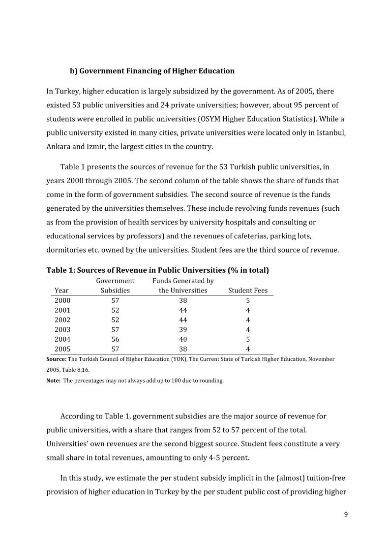
Table 1 presents the sources of revenue for the 53 Turkish public universities, in

years 2000 through 2005. The second column of the table shows the share of funds that

come in the form of government subsidies. The second source of revenue is the funds

generated by the universities themselves. These include revolving funds revenues (such

as from the provision of health services by university hospitals and consulting or

educational services by professors) and the revenues of cafeterias, parking lots,

dormitories etc. owned by the universities. Student fees are the third source of revenue.

Table 1: Sources of Revenue in Public Universities (% in total)

Year

Government

Subsidies

Funds Generated by

the Universities

Student Fees

2000 57 38 5

2001 52 44 4

2002 52 44 4

2003 57 39 4

2004 56 40 5

2005 57 38 4

Source: The Turkish Council of Higher Education (YOK), The Current State of Turkish Higher Education, November

2005, Table 8.16.

Note: The percentages may not always add up to 100 due to rounding.

According to Table 1, government subsidies are the major source of revenue for

public universities, with a share that ranges from 52 to 57 percent of the total.

Universities’ own revenues are the second biggest source. Student fees constitute a very

small share in total revenues, amounting to only 4-5 percent.

In this study, we estimate the per student subsidy implicit in the (almost) tuition-free

provision of higher education in Turkey by the per student public cost of providing higher

10

education. This is calculated by dividing the total recurrent expenditures of faculties (i.e.

the funds allocated from the national budget to cover the usual overall cost of providing

educational services) by the number of students enrolled in those faculties. The data

section presents a more detailed definition.

There were a total of 1,256,920 undergraduate students (excluding open university-

distance education-students) enrolled in the 53 public universities in year 2005. The

average per student subsidy in our data is 2,713 TL. However there is non-negligible

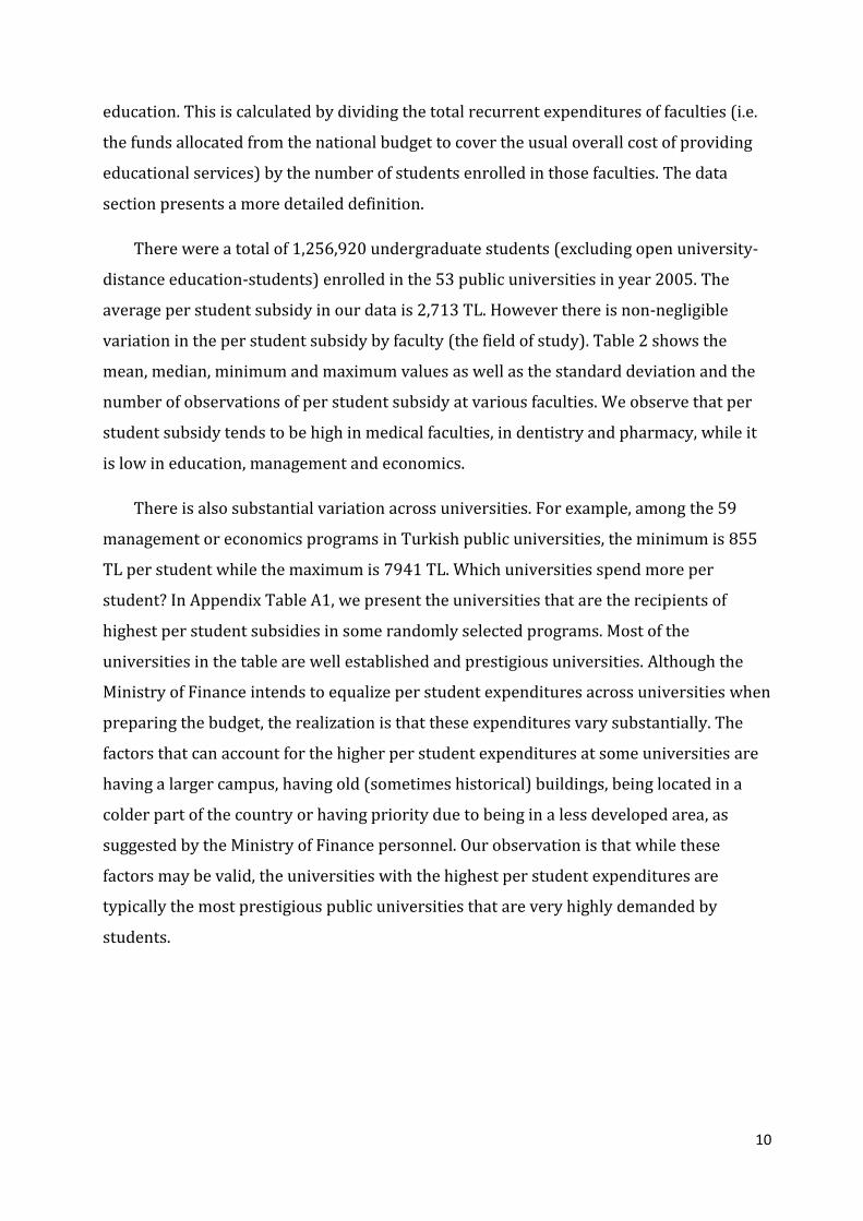
variation in the per student subsidy by faculty (the field of study). Table 2 shows the

mean, median, minimum and maximum values as well as the standard deviation and the

number of observations of per student subsidy at various faculties. We observe that per

student subsidy tends to be high in medical faculties, in dentistry and pharmacy, while it

is low in education, management and economics.

There is also substantial variation across universities. For example, among the 59

management or economics programs in Turkish public universities, the minimum is 855

TL per student while the maximum is 7941 TL. Which universities spend more per

student? In Appendix Table A1, we present the universities that are the recipients of

highest per student subsidies in some randomly selected programs. Most of the

universities in the table are well established and prestigious universities. Although the

Ministry of Finance intends to equalize per student expenditures across universities when

preparing the budget, the realization is that these expenditures vary substantially. The

factors that can account for the higher per student expenditures at some universities are

having a larger campus, having old (sometimes historical) buildings, being located in a

colder part of the country or having priority due to being in a less developed area, as

suggested by the Ministry of Finance personnel. Our observation is that while these

factors may be valid, the universities with the highest per student expenditures are

typically the most prestigious public universities that are very highly demanded by

students.

11

Table 2: Per student subsidy at some faculties (TL per student, 2005 prices)

Mean Median Minimum Maximum StDev N

Medicine 20300 19961 1702 10578 2100 37

Dentistry, Pharmacy 8395 19961 566 68306 10793 25

Faculty of Arts and Science 3266 2464 1016 16360 2531 65

Engineering, Architecture 3979 2939 1701 14814 2527 71

Law 3235 2750 1087 8586 1950 14

Management, Economics 2318 1841 855 7941 1403 59

Fine Arts, Literature, History 3769 3524 1473 9172 1515 27

Education 2068 1839 1120 6757 937 63

Source: Authors’ calculations based on Ministry of Finance and OSYM data.

Notes: The number of observations (N) may exceed the total number of public universities in year 2005, which was 53,

in cases where there are more than one faculty in the same university. For example, if a university has both an

engineering and an architecture faculty, that university is counted twice in the “Engineering, Architecture” faculty

group.

Another important observation is the small enrollment fees charged by public

universities. The annual fees varied from 147 TL to 458 TL per student in 2005,

depending on the major of study1. The highest fees were paid by students in medicine,

dentistry, pharmacy and state conservatory for the arts. It is clear that students at public

universities in Turkey pay only a small share of the cost of higher education, in other

words they contribute very little to cost recovery. In private universities, whose main

source of revenue is tuition fees, students paid as much as 26,500 TL (Turkish Liras) and

as little as 4,266 TL annually in 2005.2

4. The Data

The data used in this study come from two main national sources: (1) the university

entrance exam data, provided by the OSYM and (2) data on the funds allocated to public

universities from the national budget, provided by the Ministry of Finance (MOF).

There is only one dataset available in Turkey that includes both the applicants’ and

their families’ characteristics. This unique dataset from year 2002 combines the

1 Authors’ calculations based on fee information from the University Entrance Exam Application Booklet, year

2005, OSYM. The average US$/TL exchange rate in 2005 was 1 USD=1.34 TL. Thus, 147 TL and 458 TL are

about US$ 110 and 342, respectively. 2 Based on the 1 USD=1.34 TL exchange rate in 2005, the highest fee was US$ 19,776 and the smallest was US$

3,184.

12

information from the students’ application documents with the information from a

number of survey questions that the students were asked to answer at the time of their

applications. The dataset was provided by the OSYM of Turkey and it contains one

random sample from each of the four high-school fields; Science, Turkish-Math (TM),

Social Sciences and Foreign Languages. Each sample contains data on about 40,000

students. We pool the four samples and hence use the data from all four high-school

fields. In the OSS data, for each student we have his OSS scores, the student’s choice list

which includes the codes of program-university pairs that the student ranks in his list,

whether the student entered university and if so, the program-university pair that he was

admitted to. In 2002, there were about a hundred different four year degree programs.

Our dataset also includes information on family and individual characteristics such as

the gender of the student, the number of children in the family, education of the parents,

employment and social security status of the parents, family income (in terms of income

brackets), expenditures on private tutoring to prepare for the exam, the number of times

that the student has taken the exam and population of the area that student attended high

school. The data on the socio-economic background of the students were collected via a

survey of the students registering to take the OSS.

We merge the OSS data with the per student subsidy data which come from the MOF.

The merge is done by the code of the program-university pair that the student is admitted

to. With this merger, we are able to tell how much per student subsidy each student

receives if he is admitted to university. We exclude students who were admitted to Open

University programs since these are part-time distance education programs with very low

per student subsidies. We also exclude students at evening programs, since we cannot

calculate the per student subsidy received by these students based on the data that we

have. Students enrolled in either type of programs have usually jobs and careers. These

restrictions bring the dataset down to 93266 observations.

The per-student subsidy calculations in this study are based on the data from the

final accounts of public universities for year 2005, the closest year to 2002 for which

detailed data could be obtained from the MOF. These data include budget realizations of

expenditures of public universities. The data are organized in economic and institutional

classification as explained below.

13

In the MOF data, total expenditures of public universities are broken down into the

following economic categories: (1) Personnel expenditures; (2) Government premium

payments to social security agencies; (3) Purchase of goods and services (includes office

equipment, stationary, periodicals, utilities, small repair and maintenance, materials for

laboratory experiments, travel allowances, etc.); (4) Current transfers (includes payments

to retirees, treatment of students in university medical center, etc.); (5) Capital

expenditures (includes new construction, major repair and maintenance, lump-sum

purchases of books and journals, real estate purchases, etc.). As part of capital

expenditures, there are some items which are large but happen once in a lifetime, such as

real estate purchases. These items are subtracted from the total; all other items constitute

the recurrent expenditures of a university, in other words they are the expenditures that

are essential for the continuation of educational activities at the university.

Important for our study, we can also see the breakdown of recurrent expenditures

by institutional divisions, which can be grouped into administrative (such as the

President’s Office, Personnel Department) and academic divisions (faculties). The

administrative divisions do not have educational functions; however their existence is

essential for a university to function properly. Therefore their expenditures are

distributed to faculties, in proportion to the shares of the faculties in total recurrent

expenditures of all academic divisions. In other words, the subsidy allocated from the

national budget to an academic division of a university is defined as the total recurrent

expenditures of the academic division plus its estimated share in total administrative

recurrent expenditures. Per student subsidy is this total amount divided by the number of

students in the academic division.

An advantage of the MOF data is that we can identify the per student subsidy not

only at the university level but also at the faculty level. This is important, since previous

studies estimate per student subsidy very roughly and only at the national level (by

dividing the total higher education expenses by the total number of students) and

therefore overlook the variation in per student subsidy across universities and faculties.

We assume that students of all departments at a faculty (for example all Engineering

students at a Faculty of Engineering) receive the same per student subsidy, since we do

not have data on expenditures at the departmental level.

14

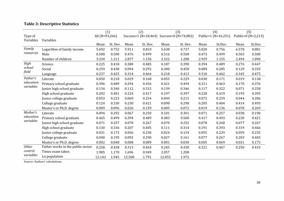
The descriptive statistics of the data used in the econometric analysis are reported

in Table 3. The dummy variables for parental education are illiterate, literate, primary

school graduate (5 years of schooling), junior high school graduate (8 years of schooling),

high school graduate (11 years of schooling), junior college graduate (2 years of

vocational college), college graduate (4-6 years of college) and master’s or Ph.D. degree,

respectively. The other variables shown in Table 3 are the logarithm of family income3,

male (equal to 1 if the student is male and 0 if female), the number of children in the

family, the student’s high school field, a dummy variable for whether the father is

affiliated with the public sector, the number of times the student has taken the exam (1 if

it is the first time, 2 if it is the second time and so on), and the logarithm of the population

of the area in which the student went to high school.

In the first part of the table we show the means and standard deviations of our

control variables for the entire sample. In the second and third parts of the table we show

the statistics for the sample of students who were successful in the exam and who were

not, respectively. It seems that successful students come from families with higher

income, fewer children and better educated parents. Within the group of successful

students, 23 percent have a college graduate father, whereas the fathers of unsuccessful

students are mostly primary school graduates (only 9.8 percent of unsuccessful students

have college graduate fathers). The corresponding figures for mothers are 9.2 percent and

2.7 percent. Successful students appear to come from bigger cities. Repeat-taking is very

common in Turkey; an average successful student has taken the exam 1.6 times, an

unsuccessful one has taken the exam about two times. There is evidence that a student’s

field choice in the high school may be correlated with his exam success. Although the four

fields are quite evenly distributed in the whole sample, 38 percent of successful students

come from the science field. The fathers of successful students are more likely to be

employed in (or retired from) the public sector.4

3 In January 2005, 6 zeros were omitted from the Turkish currency unit. We express 2002 monetary values without

the 6 zeros. 4 Public sector employment is known to offer job security and stability. According to the Turkish social security

system valid in 2002, a person was either covered by the public sector program (called Emekli Sandigi), covered

by a private sector program (called SSK or Bag-kur), or not covered at all. The public sector social security

program offers the most generous retirement and health benefits (Caner and Okten (2010)).

15

In the fourth and fifth parts of the table, we restrict the sample to those who were

successful in the exam and compare the students who were placed at a public university

to those who were placed at a private university. Students who go to private universities

in Turkey seem to come from higher income families as opposed to those who go to public

ones. They also have better educated parents. About 7.8 percent of private university

students have fathers with a master’s or Ph.D. degree, while only 1.9 percent of public

university students do. The corresponding figures for mothers’ education are 20.3

percent versus 7.7 percent. The students who are placed at a public university appear

more likely to have fathers who are public sector employees than private university

students (32.1 percent versus 25 percent). Students that are placed in private universities

seem less likely to be in the science field and more likely to be in the social field indicating

possible specialization of private universities in certain fields.

We conduct t-tests on the equality of means of two groups. Comparing those who

were placed at a public university to those who were placed at a private university, the

hypothesis of the equality of mean family incomes is rejected with a very small p-value

(t=43.28). Similarly, those who were placed at a public university had higher mean family

income when compared to those who failed in the exam, again with a very small p-value

(t=28.75). These findings tell us that private university students come from higher income

families than public university students and that public university students are richer

than those who failed in the exam, without controlling for any other factor.

16

Table 3: Descriptive Statistics

Type of Variables

(1) All (N=93,266)

(2) Success=1 (N=18,464)

(3) Success=0 (N=74,802)

(4) Public=1 (N=16,251)

(5) Public=0 (N=2,213)

Variables Mean St. Dev. Mean St. Dev. Mean St. Dev. Mean St.Dev. Mean St.Dev.

Family resources

Logarithm of family income 5.692 0.752 5.911 0.810 5.638 0.727 5.820 0.756 6.578 0.881

Male 0.508 0.500 0.476 0.499 0.516 0.500 0.473 0.499 0.503 0.500

Number of children 3.234 1.211 2.877 1.156 3.322 1.208 2.929 1.155 2.494 1.090 High school field

Science 0.225 0.418 0.380 0.485 0.187 0.390 0.394 0.489 0.276 0.447

Social 0.259 0.438 0.094 0.292 0.300 0.458 0.089 0.285 0.129 0.335

Language 0.237 0.425 0.314 0.464 0.218 0.413 0.310 0.462 0.345 0.475 Father’s education variables

Literate 0.050 0.218 0.029 0.168 0.055 0.229 0.030 0.171 0.019 0.138

Primary school graduate 0.396 0.489 0.294 0.456 0.421 0.494 0.311 0.463 0.170 0.376

Junior high school graduate 0.134 0.340 0.112 0.315 0.139 0.346 0.117 0.322 0.071 0.258

High school graduate 0.202 0.401 0.224 0.417 0.197 0.397 0.228 0.419 0.193 0.395

Junior college graduate 0.053 0.223 0.069 0.254 0.049 0.215 0.072 0.259 0.044 0.206

College graduate 0.124 0.330 0.230 0.421 0.098 0.298 0.205 0.404 0.414 0.493

Master’s or Ph.D. degree 0.009 0.096 0.026 0.159 0.005 0.072 0.019 0.136 0.078 0.269 Mother’s education variables

Literate 0.094 0.292 0.067 0.250 0.101 0.301 0.071 0.257 0.038 0.190

Primary school graduate 0.465 0.499 0.394 0.489 0.483 0.500 0.417 0.493 0.230 0.421

Junior high school graduate 0.071 0.257 0.078 0.267 0.070 0.255 0.078 0.268 0.077 0.267

High school graduate 0.130 0.336 0.207 0.405 0.111 0.314 0.191 0.393 0.319 0.466

Junior college graduate 0.031 0.172 0.056 0.230 0.024 0.154 0.055 0.229 0.059 0.235

College graduate 0.040 0.195 0.092 0.290 0.027 0.161 0.077 0.267 0.203 0.403

Master’s or Ph.D. degree 0.002 0.048 0.008 0.089 0.001 0.030 0.005 0.069 0.031 0.173 Other control variables

Father works in the public sector 0.258 0.438 0.313 0.464 0.245 0.430 0.321 0.467 0.250 0.433 Times exam taken 1.985 1.170 1.696 0.949 2.057 1.208

Ln population 12.143 1.945 12.500 1.791 12.055 1.972 Source: Authors’ calculations.

17

5. Econometric framework

We conceptualize the decision-making process of a student as follows: The student takes

the OSS exam and observes his score. If he earns a score high enough to be admitted to a

university, he decides whether he prefers to attend a public or a private university based

on his own characteristics and his preferences for what these universities have to offer. If

a student goes to a public university, he receives an implicit education subsidy from the

government. We are interested in finding out the characteristics of students who have

been successful in the exam, who go to public versus private universities and the

characteristics of students who receive a high subsidy.

We estimate two models: a three stage Heckman selection model and a three-part model.

We explain the selection model first. In the first stage of the model the outcome variable

“s” is success at the university entrance exam where the student earns the right to be

placed at a program-university pair. We estimate this by a probit equation where the

dependent variable “s” takes the value of 1 if the student is successful at the university

entrance exam and earns the right to be placed at a program-university pair as a result of

his university exam score and preference list.

, {

(for the entire sample) (1)

In the second stage, we look at the sample of students who were successful in the

exam. The outcome variable “p” is placement at a public university. We estimate a probit

equation where “p” takes the value of 1 if the student was placed at a public university

and 0 if placed at a private university as a result of his preference list and exam score. To

control for the possible effect of selection into “success”, we use the inverse Mills ratio

from the first stage as an explanatory variable in the second stage probit.

{

(for the subsample ) (2)

In stage three, the outcome “c” is the recurrent expenditures of the program-

university pair which indicates the amount of subsidy received by each student from the

government. We call this variable the “subsidy per student”. We observe this variable only

for public universities; hence at this stage our sample is restricted to students who

18

entered a public university. To control for the possible effect of selection into “public

university”, we use the inverse Mills ratio from the second stage in this regression.

(for the subsample ) (3)

The matrix includes:

(1) income measures, we use two alternative income measures in our estimations:

a) “lnincome” variable: In the survey, applicants are asked to choose one of the seven

family income brackets. Hence, we generate an income variable that is equal to the

midpoint of the income bracket chosen and use the natural logarithm of this variable as a

measure of family income in our regressions.

b) income dummy variables: In order to capture the non-linear effects of income (and also

not to impose any artificial income distances between applicants as is the case with the

midpoint method), we generate four income dummy variables based on income

percentiles5 as explained in Section 6.

(2) “male” dummy variable, which is equal to one if the student is male, zero otherwise,

(3) the “number of children” variable that indicates the number of children in the

family,

(4) the “science”, “social” and “language” dummy variables that indicate the high school

field of the student (the omitted category is “Turkish and mathematics”),

(5) seven dummy variables for father’s education, as explained in Section 4; the omitted

category for education is illiterate,

(6) seven similarly defined dummies for mother’s education.

The matrix includes all variables in matrix besides a dummy variable that

indicates whether the student’s father works in the public sector. This variable is used as

an exclusion restriction in the per student subsidy equation in stage 3. We assume that

this variable affects the student’s preference towards getting an education from a public

university, but has no direct effect on the subsidy she receives from the public university. 5 The categorical monthly family income variable takes seven values (less than 250 TL, 200-500 TL, 500-750 TL,

750-1000 TL, 1000-1500 TL, 1500-2000 TL and more than 2000 TL). The “Income1” dummy is one for the

lowest income group (37% of the population), “Income2” dummy is one for the 200-500 TL group (40% of the

population), “Income3” dummy is one for 500-750 TL (13% of the population) and “Income4” dummy is one for

more than 750 TL income group (the richest 10% of the population). The highest three income brackets are

grouped into Income4 dummy variable due to their low observation frequency.

19

Caner and Okten (2010) find that in Turkey, students whose fathers are public sector

employees are more likely to choose majors that lead to careers in the public sector.

The matrix includes all variables in matrix besides two variables. The first of

these variables is “lnpopulation”, defined as the logarithm of the population of the area in

which the student went to high school. The population variable is used as an indicator of

the learning resources (such as high quality schools, private tutoring centers, libraries

etc.) that the student has access to while in high school. The other is “times exam taken”,

defined as the number of times that the student has taken the exam. The “times exam

taken” variable is considered as a regressor in the first stage since it influences the

chances of success via two channels: first, repeaters may be less able students, second,

repeaters may be more willing to enter university and make their choices accordingly,

while first time exam takers may be more comfortable with taking the risk of failure and

may target highly demanded programs. Therefore, the direction of influence on success is

ambiguous.

These variables are used as exclusion restrictions in the public university equation

in stage 2. Our assumption here is that these variables affect the student’s probability of

success in the exam, but have no direct effect on the probability that she is placed at a

public university.6

We next explain our choice of the variables in matrix X3 which are also used as

explanatory variables in the first two stages. One of our main interests is to find out how

the financial resources of the family affect a student’s chances of receiving higher

education. We include family income and number of children in the family variables in our

regressions, both of which determine the amount of resources that are available to the

student.

We control for the gender of the student because both the success in the exam and

the preference towards a private university can be influenced by this characteristic. There

is a large literature on son preference and its consequences on children’s mortality and

6 One can develop arguments against this assumption and argue that our exclusion restrictions are weak in

controlling for selection. For example, the “lnpopulation” variable might have a direct effect on preferences for a

private versus a public university since private universities were located only in the three largest cities in 2002.

Similarly, if repeat takers prefer to wait and retake the exam in order to have another chance to be admitted to a

well-known public university, the “times exam taken” variable might have a direct effect on preferences for a

public university in addition to its indirect effect via success in the exam.

20

educational achievements. These studies list the social, cultural and economic reasons

behind such a preference. Rosenzweig and Schultz (1982) find that children who are

anticipated to be more economically productive adults receive a larger share of family

resources and have a greater chance to survive. Recent studies on China provide

alternative explanations for the higher than normal male-female ratio in the country, two

of which are the practices of sex selective abortion and infanticide by the parents

(Ebenstein, 2010). Tansel (2002) finds a larger effect of family income on schooling of

girls than that of boys in primary and secondary education in Turkey, and interprets that

this finding could be due to a taste effect as much as a more effective income constraint

for girls than for boys. Based on these, we include the gender control in our regressions to

account for the possibility that the willingness to pay for the education of a son is greater

than that of a daughter, which would affect both the exam success of a student and the

likelihood of attending a private university by influencing the amount of family resources

devoted to male children.

Parental education variables are included in the regressions as they are considered

to be good indicators of both ability and socioeconomic status. Income is another

indicator of socioeconomic status, and probably of ability; however there are reasons to

prefer education as a measure of the social position of a student’s family. As written by

Lemelin (1992, p.178), “First, education and social position are highly correlated;

education has been used to estimate permanent income in economics, and social prestige

of occupation in sociology. Second, it can be assumed that the education level of parents is

better known than their income by university students.”

The controls for the student’s high school field (“Science”, “Social” and “Language”)

are included since there might be selection at the time the student chooses his high school

field and these variables might affect the probability of success. The omitted field is the

Turkish-Math (TM) field. For instance, higher ability students might choose to be in the

“Science” field while others may prefer the broader “Social Science” or “Turkish-Math”

fields. It is likely that only students who are genuinely interested in languages choose to

be in the “Language” field. These variables can also influence the student’s public

university choice since all majors are offered by public universities whereas private

universities may choose to specialize in certain programs. For instance, economics and

21

business majors are offered by almost all private universities, whereas civil engineering

programs are mostly offered by public universities in Turkey.

Per student subsidy also differs across fields. Programs such as medical school and

engineering where students with science fields are mostly placed may be categorically

more expensive and hence receive higher subsidies than programs such as economics and

business where students with TM fields are mostly enrolled. Hence including field

dummies in the third stage per student subsidy regression might underestimate the effect

of income on placement in higher subsidy programs. Therefore we also present the third

stage regression where the X3 matrix does not include field dummies.

In studies related to ours, researchers have used the “two-part model” to estimate

similar equations. For example, Liu et al. (2006) estimate a model that consists of two

equations, the first of which explains the probability of attending a college or university

and the second of which explains the conditional probability that a potential college

student will attend a public university. They state that they have no good exclusion

restrictions and therefore estimate these equations by using the “two-part model” as in

Leung and Yu (1996) instead of the Heckman type selection model. Although we do have

good candidates for exclusion restrictions, we supplement our results from the selection

model with the estimates from a “three-part model” for two reasons. One is comparability

with the literature. The other is the ease of computing the overall marginal effects from

the three-part model. The selection model yields the marginal effects at each step

separately; the three-part model can be used to compute the overall impact of a small

change in an explanatory variable on per student subsidy received by an average exam

taker in the country.

The model consists of the same three equations (1)-(3) described above, except that

there is no selection correction. The equations are estimated separately, equations (1)

and (2) by probit and (3) by OLS. The expected value of per student subsidy among exam

takers is expressed as the product of the probability of success, the probability of public

university attendance among those who succeed in the exam and the expected value of

per student subsidy among those attending a public university:

( ) ( ) ( ) , (4)

where ( ) shows the cumulative normal distribution function.

22

With the three-part model, we can estimate the marginal effects easily without

having to deal with the selection correction terms. We derive the marginal effect of each

independent variable in a similar way to Dow and Norton (2003), by taking the derivative

of the expected value of per student subsidy with respect to the particular explanatory

variable. The marginal effect of a variable is expressed as the following and estimated

at sample averages:

( )

( ) ( ) ( ) { ( ) ( ) } (5)

where ( ) shows the normal density function and ( ) shows the cumulative normal

distribution function. We estimate the standard errors of these marginal effects via

bootstrapping with 50 replications. As indicated before, these marginal effects tell us the

overall impact of a small change in an explanatory variable on per student subsidy

received by an average exam taker in the country.

6. Results and Discussion

a. The Three-Stage Heckman Model

We estimate a three-stage Heckman selection model. In the first stage, we estimate

equation (1) by probit. In our first set of results we use the natural logarithm of family

income which is constructed using the midpoints of the seven family income brackets that

applicants were asked to choose from. In Table 4, we observe that family income has a

positive and statistically significant effect on university entrance (column 1a). An

approximately ten percent increase in family income increases the probability of

university entrance by ten percentage points (column 1c). Number of children in the

family as a measure of resources available to the student has a negative and significant

effect on the probability of success while sex of the student does not have a statistically

significant effect.

Both father’s and mother’s education levels appear to be very important

determinants of university entrance. As compared to students whose parents received a

junior high school education or less, students whose mothers received a high school

education were 4.7 percentage points more likely to enter university, those whose fathers

23

had a high school degree were 1.7 percentage points more likely to enter university. As

compared to students whose parents received a high school education or less, students

whose mothers received a four year college education were 5.6 percentage points more

likely to enter university, those whose fathers had a college degree were 7 percentage

points more likely to enter university. Similar to existing studies on human capital (Liu et

al. (2006), Haveman and Wolfe (1995), Behrman (1999)), we also find that in general

mother’s education level is economically more significant than father’s educational

attainment. However we fail to reject the equality of father’s and mother’s relevant

educational attainments in all categories except for high school graduates in statistical

tests of relevant coefficients.

Number of times exam taken has a negative and significant effect on success in

university entrance and hence we interpret this variable as a measure of ability. As

expected, the population of the city where the student went to high school has a positive

and significant effect. Population is a relevant measure of availability of private tutoring

centers that help students prepare for the university entrance exam and quality of high

schools. These variables are also our exclusion restrictions and hence excluded from the

second stage probit. We tested the joint significance of these two variables in our first

stage regression and found that they are jointly significant with a Chi-square distributed

Wald test statistic of 313.79 and a p-value that is almost zero.

In the second stage, the outcome is entering a public university. We estimate

equation (2) by probit. We observe this outcome for students that have succeeded in the

university entrance exam. Hence we use the inverse Mills ratio (mills1) from the first

stage as an explanatory variable in the second stage probit. In Table 4, columns (2a)

through (2c), we present these results. We observe that contrary to the results in Liu et al.

(2006), students from higher income families are more likely to go to private universities.

A one percent increase in family income decreases the probability of going to a public

university by 9 percentage points. This is a positive result in terms of public policy. We

attribute the difference in findings from Liu et al. (2006) to the lack of price regulation in

Turkish private higher education sector and the existence of price controls in the

Taiwanese private higher education market. The Turkish private higher education sector

is able to provide a product that is perceived to be of high quality and hence attracts

24

students from high income families. This finding contradicts also with Rozada and

Menendez (2002) study on Argentina where public and private university students have

the same characteristics and both come from the highest income families. Another finding

is that, as expected, students that come from families with more children are more likely

to go to public universities than private ones, since the number of children in the family

decreases per student resource availability. Interestingly, male students are more likely to

go to private universities rather than private ones. This result is consistent with the

earlier results in the literature on families’ willingness to expend more resources on male

children.

We also observe that students whose parents have high educational attainment are

more likely to go to private universities. As compared to students whose mothers

received only a primary school education degree, students whose mothers received a four

year bachelor’s degree are 16.6 percentage points more likely to enter a private

university than a public university (Table 4, column 2c). The finding that students from

high income, high education families are more likely to enter private universities implies

that these universities are prestigious. These universities offer tuition-free education to a

small group of students (based on merit) while charging the full tuition to the majority of

their students. The existence of such a group is expected to motivate others to study

harder. We exclude these few students from our sample since they neither receive an

implicit government subsidy nor pay for the tuition. We deduce that the combined effect

of the existence of this group of students and the lack of price-ceilings on the tuition fees

charged by private universities help maintain the quality of education provided by these

institutions.

Interestingly, father’s public sector employment status increases the probability of

entering a public university as opposed to a private university by 7.2 percentage points

(Table 4, column 2c) although its effect on success at university entrance was negative

and significant (Table 4, column 1a). This result seems to support our assumption that

that father’s public sector status affects the student’s preference towards getting an

education from a public university.

25

Table 4: Regression results on university attendance and public university

attendance

University entrance Public University

Type of Variables

Variables Coef.

Robust Std. Err.

Marg. effect Coef.

Robust Std. Err.

Marg. effect

(1a) (1b) (1c) (2a) (2b) (2c) Family resources

Lnincome 0.037 *** 0.008 0.010 -0.585 *** 0.025 -0.090

Male -0.010 0.01 -0.003 -0.181 *** 0.028 -0.028

Number of children -0.047 *** 0.005 -0.012 0.058 *** 0.019 0.009 High school field

Science 0.529 *** 0.013 0.153 -0.236 ** 0.102 -0.038

Social -0.280 *** 0.016 -0.067 0.099 0.088 0.014

Language 0.357 *** 0.014 0.100 -0.325 *** 0.077 -0.055 Father’s education variables

Literate 0.005 0.043 0.001 -0.010 0.149 -0.002

Primary school graduate 0.036 0.036 0.009 0.153 0.132 0.023

Junior high school graduate 0.062 * 0.039 0.016 0.121 0.139 0.018

High school graduate 0.123 *** 0.038 0.033 0.028 0.139 0.004

Junior college graduate 0.199 *** 0.044 0.055 -0.067 0.152 -0.011

College graduate 0.358 *** 0.041 0.103 -0.520 *** 0.154 -0.097

Master’s or Ph.D. degree 0.613 *** 0.061 0.197 -0.977 *** 0.187 -0.255 Mother’s education variables

Literate 0.007 0.023 0.002 -0.142 ** 0.083 -0.024

Primary school graduate 0.023 0.018 0.006 -0.193 *** 0.069 -0.031

Junior high school graduate 0.054 ** 0.026 0.014 -0.358 *** 0.085 -0.067

High school graduate 0.220 *** 0.024 0.061 -0.658 *** 0.091 -0.131

Junior college graduate 0.294 *** 0.033 0.085 -0.540 *** 0.11 -0.113

College graduate 0.391 *** 0.032 0.117 -0.841 *** 0.114 -0.197

Master’s or Ph.D. degree 0.745 *** 0.098 0.249 -1.413 *** 0.184 -0.427 Other control variables

Father's public sector status -0.086 *** 0.013 -0.022 0.529 *** 0.038 0.072 Number of times exam taken -0.076 *** 0.005 -0.020

Lnpopulation 0.020 *** 0.003 0.005

Constant -1.373 *** 0.065

7.084 *** 0.476 Mills1

-1.478 *** 0.241

Chi/F squared 8100.7

1749.77

log likelihood -41693

-5597.5

R-squared 0.1

0.173

Number of observations 93266

18464

Source: Authors’ calculations.

Notes: “Coef.” is the estimated coefficient, “Robust Std.Err.” is the robust standard error of the coefficient, “Marg.effect”

is the marginal effect of an explanatory variable on the dependent variable.

26

Table 5: Regression results on per-student subsidy (with and without high school

field dummy variables)

Type of Variables

Dependent Variable: Per-student Subsidy

Robust Std. Err.

Robust Std. Err. Variables Coef. dlny/dx Coef. dlny/dx

(1) (2) (3) (4) (5) (6)

Family resources

Lnincome 298.566 *** 62.967 0.086 953.499 *** 59.88 0.277

Male 169.184 *** 56.623 0.049 666.551 *** 55.426 0.194

Number of children 73.205 *** 26.939 0.021 74.136 *** 27.644 0.022 High school field

Science 2099.501 *** 64.672 0.610

Social 463.89 *** 49.018 0.134

Language 451.857 *** 32.582 0.131 Father’s

education variables

Literate -88.592 225.526 -0.025 -32.987 228.767 -0.010

Primary school graduate -170.954 206.097 -0.049 -327.585 * 209.391 -0.095 Junior high school graduate -264.935 213.861 -0.077 -526.296 *** 217.719 -0.153

High school graduate -137.612 217.117 -0.04 -461.795 ** 220.587 -0.134

Junior college graduate 14.233 240.686 0.004 -442.288 ** 245.231 -0.129

College graduate 452.227 ** 224.888 0.131 511.866 ** 228.657 0.149

Master’s or Ph.D. degree 1161.356 *** 300.336 0.337 1722.781 *** 311.296 0.501 Mother’s education variables

Literate -41.717 106.384 -0.012 67.080 107.842 0.020

Primary school graduate 67.097 95.187 0.019 208.138 ** 96.535 0.061 Junior high school graduate 210.326 * 133.446 0.061 501.259 *** 135.127 0.146

High school graduate 529.784 *** 123.416 0.154 1049.655 *** 123.559 0.305

Junior college graduate 682.509 *** 168.137 0.198 835.698 *** 173.133 0.243

College graduate 933.864 *** 157.834 0.271 1622.194 *** 160.81 0.472

Master’s or Ph.D. degree 1586.767 *** 322.703 0.461 3212.429 *** 353.856 0.934 Other control variables

Father's public sector status

Number of times exam taken

Lnpopulation Constant 403.272 395.906 -1842.56 *** 385.238 Mills2 -1414.78 *** 309.612 -0.4115 -6188.51 *** 290.7828 -1.800

Chi/F squared 94.49

48.1

log likelihood

R-squared 0.112

0.061

Number of observations 16251

16251

Source: Authors’ calculations.

Notes: “Coef.” is the estimated coefficient, “Robust Std.Err.” is the robust standard error of the coefficient, “dlny/dx”

shows the derivative of the logarithm of per student subsidy with respect to each explanatory variable.

27

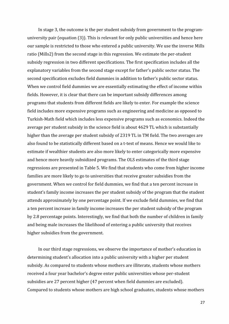
In stage 3, the outcome is the per student subsidy from government to the program-

university pair (equation (3)). This is relevant for only public universities and hence here

our sample is restricted to those who entered a public university. We use the inverse Mills

ratio (Mills2) from the second stage in this regression. We estimate the per-student

subsidy regression in two different specifications. The first specification includes all the

explanatory variables from the second stage except for father’s public sector status. The

second specification excludes field dummies in addition to father’s public sector status.

When we control field dummies we are essentially estimating the effect of income within

fields. However, it is clear that there can be important subsidy differences among

programs that students from different fields are likely to enter. For example the science

field includes more expensive programs such as engineering and medicine as opposed to

Turkish-Math field which includes less expensive programs such as economics. Indeed the

average per student subsidy in the science field is about 4629 TL which is substantially

higher than the average per student subsidy of 2319 TL in TM field. The two averages are

also found to be statistically different based on a t-test of means. Hence we would like to

estimate if wealthier students are also more likely to enter categorically more expensive

and hence more heavily subsidized programs. The OLS estimates of the third stage

regressions are presented in Table 5. We find that students who come from higher income

families are more likely to go to universities that receive greater subsidies from the

government. When we control for field dummies, we find that a ten percent increase in

student’s family income increases the per student subsidy of the program that the student

attends approximately by one percentage point. If we exclude field dummies, we find that

a ten percent increase in family income increases the per student subsidy of the program

by 2.8 percentage points. Interestingly, we find that both the number of children in family

and being male increases the likelihood of entering a public university that receives

higher subsidies from the government.

In our third stage regressions, we observe the importance of mother’s education in

determining student’s allocation into a public university with a higher per student

subsidy. As compared to students whose mothers are illiterate, students whose mothers

received a four year bachelor’s degree enter public universities whose per-student

subsidies are 27 percent higher (47 percent when field dummies are excluded).

Compared to students whose mothers are high school graduates, students whose mothers

28

received a four year bachelor’s degree enter public universities whose per-student

subsidies are 11.7 percent higher (16.7 percent when field dummies are excluded).

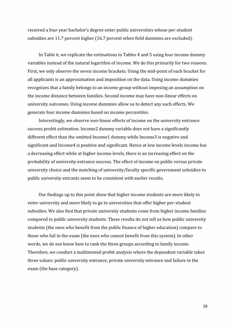
In Table 6, we replicate the estimations in Tables 4 and 5 using four income dummy

variables instead of the natural logarithm of income. We do this primarily for two reasons.

First, we only observe the seven income brackets. Using the mid-point of each bracket for

all applicants is an approximation and imposition on the data. Using income dummies

recognizes that a family belongs to an income group without imposing an assumption on

the income distance between families. Second income may have non-linear effects on

university outcomes. Using income dummies allow us to detect any such effects. We

generate four income dummies based on income percentiles.

Interestingly, we observe non-linear effects of income on the university entrance

success probit estimation. Income2 dummy variable does not have a significantly

different effect than the omitted Income1 dummy while Income3 is negative and

significant and Income4 is positive and significant. Hence at low income levels income has

a decreasing effect while at higher income levels, there is an increasing effect on the

probability of university entrance success. The effect of income on public versus private

university choice and the matching of university/faculty specific government subsidies to

public university entrants seem to be consistent with earlier results.

Our findings up to this point show that higher income students are more likely to

enter university and more likely to go to universities that offer higher per-student

subsidies. We also find that private university students come from higher income families

compared to public university students. These results do not tell us how public university

students (the ones who benefit from the public finance of higher education) compare to

those who fail in the exam (the ones who cannot benefit from this system). In other

words, we do not know how to rank the three groups according to family income.

Therefore, we conduct a multinomial probit analysis where the dependent variable takes

three values: public university entrance, private university entrance and failure in the

exam (the base category).

29

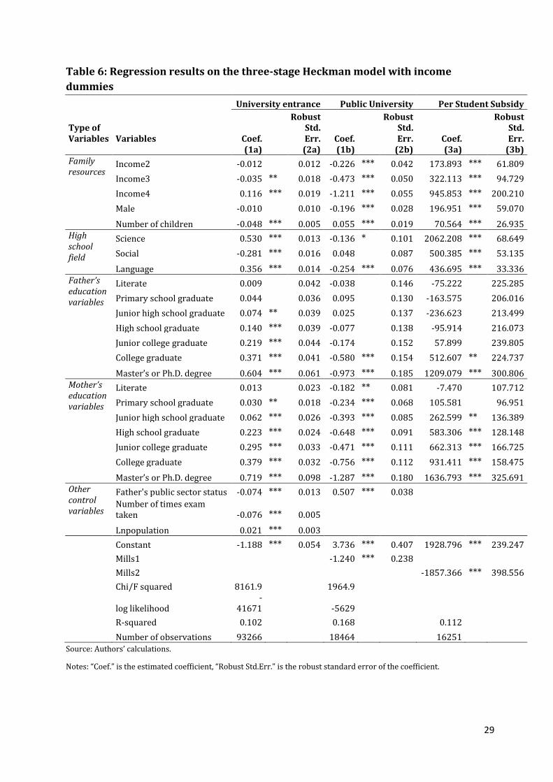
Table 6: Regression results on the three-stage Heckman model with income

dummies

University entrance Public University Per Student Subsidy

Type of Variables Variables Coef.

Robust Std. Err. Coef.

Robust Std. Err. Coef.

Robust Std. Err.

(1a)

(2a) (1b)

(2b) (3a)

(3b)

Family resources

Income2 -0.012

0.012 -0.226 *** 0.042 173.893 *** 61.809

Income3 -0.035 ** 0.018 -0.473 *** 0.050 322.113 *** 94.729

Income4 0.116 *** 0.019 -1.211 *** 0.055 945.853 *** 200.210

Male -0.010

0.010 -0.196 *** 0.028 196.951 *** 59.070

Number of children -0.048 *** 0.005 0.055 *** 0.019 70.564 *** 26.935 High school field

Science 0.530 *** 0.013 -0.136 * 0.101 2062.208 *** 68.649

Social -0.281 *** 0.016 0.048

0.087 500.385 *** 53.135

Language 0.356 *** 0.014 -0.254 *** 0.076 436.695 *** 33.336 Father’s education variables

Literate 0.009

0.042 -0.038

0.146 -75.222

225.285

Primary school graduate 0.044

0.036 0.095

0.130 -163.575

206.016

Junior high school graduate 0.074 ** 0.039 0.025

0.137 -236.623

213.499

High school graduate 0.140 *** 0.039 -0.077

0.138 -95.914

216.073

Junior college graduate 0.219 *** 0.044 -0.174

0.152 57.899

239.805

College graduate 0.371 *** 0.041 -0.580 *** 0.154 512.607 ** 224.737

Master’s or Ph.D. degree 0.604 *** 0.061 -0.973 *** 0.185 1209.079 *** 300.806 Mother’s education variables

Literate 0.013

0.023 -0.182 ** 0.081 -7.470

107.712

Primary school graduate 0.030 ** 0.018 -0.234 *** 0.068 105.581

96.951

Junior high school graduate 0.062 *** 0.026 -0.393 *** 0.085 262.599 ** 136.389

High school graduate 0.223 *** 0.024 -0.648 *** 0.091 583.306 *** 128.148

Junior college graduate 0.295 *** 0.033 -0.471 *** 0.111 662.313 *** 166.725

College graduate 0.379 *** 0.032 -0.756 *** 0.112 931.411 *** 158.475

Master’s or Ph.D. degree 0.719 *** 0.098 -1.287 *** 0.180 1636.793 *** 325.691 Other control variables

Father's public sector status -0.074 *** 0.013 0.507 *** 0.038 Number of times exam

taken -0.076 *** 0.005

Lnpopulation 0.021 *** 0.003 Constant -1.188 *** 0.054 3.736 *** 0.407 1928.796 *** 239.247

Mills1

-1.240 *** 0.238 Mills2

-1857.366 *** 398.556

Chi/F squared 8161.9

1964.9

log likelihood

-41671

-5629

R-squared 0.102

0.168

0.112

Number of observations 93266

18464

16251

Source: Authors’ calculations.

Notes: “Coef.” is the estimated coefficient, “Robust Std.Err.” is the robust standard error of the coefficient.

30

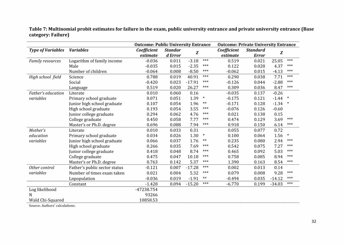
The results, presented in Table 7, tell us that on average public university students

are poorer than those who fail in the exam. So, in this sense, public provision of higher

education supports the poor families. The OSS is a great opportunity for poor but bright

and hard-working students to receive subsidized higher education. However, there are

subtleties involved. First, public universities in Turkey do not form a homogenous group.

A degree from a more prestigious public university leads to better employment

opportunities. The fact that higher income students are more likely to attend higher

subsidy and better-known universities indicate that there are regressive distributional

effects of government subsidies for higher education among their recipients. Second,

although on average public university students are poorer than those who fail in the

exam, the parents of the earlier group have more education than parents of the latter.

Since education is known as a good indicator of socio-economic status, the combined

evidence suggests that the public university system in Turkey supports students from

higher socio-economic groups.

b. The Three-Part Model

In the three stage Heckman model the Mills’ ratios were statistically significant in all

regressions, which can be taken as evidence that there is selection. However, we think

that it is worthwhile to consider an alternative approach to analyze the university

entrance problem which we will refer to as the “Three-Part Model”. This model is based

on the idea that the existence of a high number of missing values of the dependent

variables does not create a selection problem. The censoring of the dependent variable is

taken into account, but no correction is made for selection bias. As mentioned before, Liu

et al. (2006) use this method to study university choice in Taiwan.

The selection model in section 6.a shows us the effect of each explanatory variable

in each step of the model. In the three-part model we estimate the equations without any

correction for sample selection and obtain results that are qualitatively similar to the

selection model (the regression results are not presented for brevity). In addition, we

compute the marginal effects of explanatory variables using the information from all

three equations as shown by equation 5 and as explained in the econometric framework

section. The marginal effects along with their standard errors and statistical significance

31

levels are reported in Tables 8 and 9. Here, the estimated marginal effects tell us how

much a small change in an explanatory variable affects the amount of per student subsidy

received by an average OSS applicant.

In Table 8, specification A, we show the results for the model described by equations

(1)-(3). In specification B, we show the results when field dummies are excluded from

equation (3). As another analysis to complement our findings, we check for any nonlinear

effects of family income. In Table 9, we show the results using these income dummies

instead of the “logarithm of family income” variable. In Tables 8 and 9, the only difference

between the two specifications is in the field dummies in equation (3).

32

Table 7: Multinomial probit estimates for failure in the exam, public university entrance and private university entrance (Base category: Failure)

Outcome: Public University Entrance Outcome: Private University Entrance Type of Variables Variables Coefficient

estimate Standard Error

Z Coefficient

estimate Standard

Error Z

Family resources Logarithm of family income -0.036 0.011 -3.18 *** 0.519 0.021 25.05 *** Male -0.035 0.015 -2.35 *** 0.122 0.028 4.37 *** Number of children -0.064 0.008 -8.50 *** -0.062 0.015 -4.13 ***

High school field Science 0.788 0.019 40.91 *** 0.290 0.038 7.71 *** Social -0.420 0.023 -17.91 *** -0.126 0.044 -2.88 *** Language 0.519 0.020 26.27 *** 0.309 0.036 8.47 ***

Father’s education variables

Literate 0.010 0.060 0.16 -0.035 0.137 -0.26 Primary school graduate 0.071 0.051 1.39 * -0.175 0.121 -1.44 * Junior high school graduate 0.107 0.054 1.96 ** -0.171 0.128 -1.34 * High school graduate 0.193 0.054 3.55 *** -0.076 0.126 -0.60 Junior college graduate 0.294 0.062 4.76 *** 0.021 0.138 0.15 College graduate 0.450 0.058 7.77 *** 0.474 0.129 3.69 *** Master’s or Ph.D. degree 0.696 0.088 7.94 *** 0.918 0.150 6.14 ***

Mother’s education variables

Literate 0.010 0.033 0.31 0.055 0.077 0.72 Primary school graduate 0.034 0.026 1.30 * 0.100 0.064 1.56 * Junior high school graduate 0.066 0.037 1.76 ** 0.235 0.080 2.94 *** High school graduate 0.266 0.035 7.69 *** 0.542 0.075 7.27 *** Junior college graduate 0.418 0.048 8.74 *** 0.465 0.092 5.03 *** College graduate 0.475 0.047 10.18 *** 0.758 0.085 8.94 *** Master’s or Ph.D. degree 0.763 0.142 5.37 *** 1.390 0.163 8.54 ***

Other control variables

Father's public sector status -0.121 0.007 -17.28 *** 0.002 0.013 0.14 Number of times exam taken 0.021 0.004 5.32 *** 0.079 0.008 9.28 *** Lnpopulation -0.036 0.019 -1.91 ** -0.494 0.035 -14.12 ***

Constant -1.428 0.094 -15.20 *** -6.770 0.199 -34.03 *** Log likelihood -47238.754 N 93266 Wald Chi-Squared 10858.53 Source: Authors’ calculations.

33

In the three-part model, similar to the results from the selection model, we find that

parental education affects the amount of subsidy that the student receives positively and

that the effect is statistically significant when parents have at least a junior high school

degree. For example, the subsidy received by a student whose father is a college graduate

is 282.718 TL higher than a student whose father is illiterate (specification A). The

corresponding figure for the effect of the mother having a college degree is higher,

371.087 TL. In all four specifications, we notice that the mother’s education has a bigger

effect on per student subsidy.

We find that the marginal effect of family income on per student subsidy received by

an average university applicant is small and statistically insignificant. Here, we see the net

effect of three opposing forces: Students coming from higher income families, first, are

more likely to succeed in the exam; second, are less likely to attend a public university;

and third, receive a higher amount of subsidy. When the three effects are combined, the

net effect turns out to be statistically not different from zero. We observe a similar net

effect for the male dummy variable. However, the male dummy becomes statistically

significant when the field dummies are excluded, which tells us that male students choose

faculties with higher per student subsidy, such as medicine and engineering. In the case of

the number of siblings, the marginal effect is negative and statistically significant.

Although the marginal effect of family income is small and insignificant in Table 8,

the results change somewhat when we use income dummies. In Table 9, we observe the

nonlinear effect of income on per student subsidy received by an average university

applicant. We observe non-linear effects of income on per student subsidy. While dummy

variable Income2 is not statistically different from Income1, Income3 is negative and

significant while Income4 is positive and significant. In other words at the highest income

level (for the richest 10% of the population) the effect is positive and statistically

significant, which suggests that students from the highest income families are more likely

to attend universities that obtain a high amount of per student subsidy from the

government.

34

Table 8: Estimates of marginal effects in the three-part model

Specification A (with field dummies in equation (3))

Specification B (without field dummies in equation (3))

Type of Variables

Variables Coefficient estimate

Standard Error

t-ratio Coefficient

estimate Standard

Error t-ratio

Family resources

Logarithm of family income 2.136 6.826 0.313 -1.823 9.086 -0.201 Male -6.700 13.396 -0.500 41.445 14.496 2.859 *** Number of children -21.166 2.773 -7.632 *** -25.050 5.993 -4.180 ***

High school field

Science 754.053 22.303 33.810 *** 440.357 9.041 48.708 *** Social -169.490 12.757 -13.286 *** -247.114 12.474 -19.810 *** Language 332.709 5.869 56.687 *** 284.080 12.471 22.779 ***

Father’s education variables

Literate -10.522 33.981 -0.310 2.604 28.642 0.091 Primary school graduate 22.511 45.335 0.497 41.231 43.430 0.949 Junior high school graduate 17.517 65.399 0.268 42.245 47.028 0.898 High school graduate 75.005 54.559 1.375 * 111.506 46.858 2.380 *** Junior college graduate 136.859 55.255 2.477 *** 196.705 28.023 7.019 *** College graduate 282.718 41.551 6.804 *** 357.041 44.858 7.959 *** Master’s or Ph.D. degree 530.843 75.010 7.077 *** 630.987 65.036 9.702 ***

Mother’s education variables

Literate -15.267 21.703 -0.703 -2.213 23.085 -0.096 Primary school graduate 12.797 20.242 0.632 32.982 20.688 1.594 * Junior high school graduate 45.520 11.562 3.937 *** 66.577 28.198 2.361 *** High school graduate 195.746 23.413 8.361 *** 229.872 24.539 9.368 *** Junior college graduate 295.931 33.122 8.935 *** 345.512 34.551 10.000 *** College graduate 371.087 54.825 6.769 *** 432.888 30.533 14.177 *** Master’s or Ph.D. degree 662.979 85.062 7.794 *** 745.457 65.808 11.328 ***

Log likelihood -217291.98 -218034.71 N 93266 93266 Source: Authors’ calculations.

Notes: The marginal effects are calculated based on the information from all three stages of regressions, as explained in the text. Standard errors are estimated via bootstrapping.

35

Table 9: Estimates of marginal effects in the three-part model (Non-linear effects of family income)

Specification C (with field dummies in equation (3))

Specification D (without field dummies in equation (3))

Type of Variables

Variables Coefficient estimate

Standard Error

t-ratio Coefficient

estimate Standard

Error t-ratio

Family resources

Income2 -13.232 13.581 -0.974 -6.869 13.422 -0.512 Income3 -45.372 21.018 -2.159 ** -50.832 13.645 -3.725 *** Income4 40.562 16.127 2.515 *** 30.572 22.490 1.359 * Male -7.727 13.345 -0.579 40.055 9.559 4.190 *** Number of children -21.241 6.148 -3.455 *** -25.097 9.440 -2.659 ***

High school field

Science 753.716 17.263 43.660 *** 441.291 8.288 53.244 *** Social -168.820 10.730 -15.734 *** -246.076 13.138 -18.731 *** Language 331.227 9.830 33.694 *** 282.766 9.631 29.359 ***

Father’s education variables

Literate -9.232 50.296 -0.184 3.438 39.498 0.087 Primary school graduate 24.358 37.831 0.644 41.510 29.856 1.390 * Junior high school graduate 22.550 52.309 0.431 44.327 33.106 1.339 * High school graduate 83.450 35.969 2.320 *** 116.314 43.842 2.653 *** Junior college graduate 150.467 46.151 3.260 *** 205.784 50.904 4.043 *** College graduate 288.241 56.237 5.125 *** 359.025 45.304 7.925 *** Master’s or Ph.D. degree 518.439 68.520 7.566 *** 617.043 71.510 8.629 ***

Mother’s education variables

Literate -13.768 34.599 -0.398 -1.722 22.662 -0.076 Primary school graduate 14.426 18.344 0.786 33.360 17.923 1.861 ** Junior high school graduate 46.455 29.654 1.567 * 66.984 26.899 2.490 *** High school graduate 192.908 22.874 8.434 *** 227.233 20.840 10.904 *** Junior college graduate 295.333 31.975 9.236 *** 347.404 30.501 11.390 *** College graduate 357.671 29.105 12.289 *** 422.356 24.036 17.571 *** Master’s or Ph.D. degree 634.328 59.760 10.615 *** 719.503 81.878 8.787 ***

Log likelihood -219451.18 -220202.62 N 93266 93266 Source: Authors’ calculations.

Notes: The marginal effects are calculated based on the information from all three stages of regressions, as explained in the text. Standard errors are estimated via bootstrapping.

36

c. Through which channels does socio-economic background affect university

entrance and public versus private university choice?

High-school students study hard for the university entrance exam since a university

degree from a reputable university increases the chances of employment. Those who have

access to more financial resources can prepare for the exam better. In Turkey, high school

students attend tutoring centers in order to prepare for the exam. Tansel and Bircan

(2006) find that households with higher incomes and higher parental education levels

devote more resources to private tutoring using the 1994 Household Expenditure Survey.

Based on our dataset we find that private tutoring expenditures and family income are

significantly correlated with a correlation coefficient of 0.45. Furthermore, in a Tansel and

Bircan (2006) style Tobit regression where private tutoring expenditures are the

dependent variable and income and other family demographic variables are independent

variables, income is found to be positive and significant. (This regression, though not

presented for brevity, is available upon request.) Therefore, one important channel

through which having a richer family affects the probability of success in the exam is

better preparation for the exam.7

A second channel through which income may affect university entrance is the way it

shapes preferences for certain types of universities. Students from higher income families

who have more resources to prepare for the exam prefer to go to the most prestigious

public universities. In Appendix Table A1, we present the names of the universities that

offer the highest per student subsidies. Most of the universities in the table are

established and prestigious universities. Based on our observations and our experience

we know that those who are admitted to these universities have a higher chance of

obtaining a better job after graduation. Companies often list some of these universities in

their advertisements for jobs. So, we conjecture that income and other socio-economic

characteristics affect not only the probability of success but also the type of university

that a student chooses. Students with better background characteristics may have better

7 Another channel could be that income influence the quality of the high school that the student attends. Hence

family income may also play a role in tertiary level educational outcomes through its effect on secondary level

educational outcomes. Rozada and Menendez (2002) find that low income students are excluded from higher

education. We do not investigate here whether it is the case in Turkey. Such questions are beyond the scope of this

paper and warrant further research.

37

information, via a better network, on what prestigious universities have to offer; they can

have a preference for some amenities (such as social clubs and sports activities) that are

more common in well-known universities. Some students with higher income and more

educated families may prefer private universities to benefit from their smaller class sizes

and better infrastructure. Hence preferences shaped by socio-economic characteristics

also influence the university choice.

Regressions give us information about the average characteristics of different sub-

samples of students, however they do not reveal much information about the distribution

of the data and about the different groups of students within a sub-sample. To present

more evidence on this, we generate kernel density estimates of the estimated probability

of success in equation 1 (Figure 1). These probabilities are a weighted average of the

students’ characteristics in the matrix. Therefore this figure shows how students can

be grouped according to their characteristics.

Figure 1: The predicted probability of success for the three groups of students: those who are not assigned to any program, public university students and private university students (kernel density estimates)

Source: Authors’ calculations.

02

46

de

nsity

0 .2 .4 .6 .8Pr(success)

not assigned public

private

38

Comparing public university students to those who were not assigned to any

program, we see that the characteristics of many of the latter group yield a low

probability of success (Fig.1, the hump around 0.1). Most public university students have

characteristics that yield a higher probability of success (Fig. 1, the hump around 0.25).

Therefore, many public university students have different background characteristics

from those who are not assigned. Hence, this figure provides further evidence that the

publicly financed higher education system in Turkey supports the students with better

socio-economic characteristics.

We also observe in Fig.1 that there are at least two groups of public university

students (the first group represented in the hump around 0.1 and the second group

represented in the hump around 0.25). Our regression analyses imply that among public

university students higher subsidies accrue to students with better socio-economic

characteristics (i.e. characteristics that yield higher probability of success). Hence, public

university students in the second group in Fig. 1 (who have distinctly better socio-

economic characteristics compared to students who are not assigned) are the recipients

of larger public subsidies.

In our regression analyses we established that better socio-economic characteristics

increases the likelihood of going to a private university than a public one. However, it is

interesting to observe in Fig. 1 that there is considerable overlap of the curves of public

and private university entrants. In other words, there are many public university

students with characteristics that are very similar to private university students. We will

examine the public policy implications of this observation in Section 7.

d. Further robustness checks

We have established that students with higher income and more educated parents receive

higher subsidies from the government. One could argue that the amount of subsidy

offered by a public university may also be influenced by the characteristics of that

university such as its location and age. Hence, we should check whether our results will

withstand the inclusion of university specific control variables.

39

We have also established that male students are more likely to go to private

universities than public ones and among public university entrants males are more likely

to go to universities that receive higher per student subsidy from government. In a

developing and relatively traditional country such as Turkey, perhaps this result is not too

surprising. However, it does warrant further analysis of the role that gender plays in our

results. In this section, we check the robustness of our findings to university and further

gender specific control variables. Below, we show that these variables help explain the

variation in per student subsidy; but adding them to the regression does not change our

previous results qualitatively.

1. University related control variables:

In some parts of Turkey, providing education is more costly due to severe weather

conditions in long winters. The age of the university could be another important factor.

Older, historical buildings are usually more expensive to maintain. Furthermore, in large

and industrialized cities where the average cost of living is higher, one would expect labor

and material to be more expensive. To account for these effects on per student subsidy,

we add the age of the university and its square, the cost of living index and geographical

region dummies as additional control variables.

The results are presented in Table 10. There is a nonlinear (concave) relationship

between the age of the university and the subsidy per student. The effect of age is positive

for universities younger than 75-80 years, which is the case for almost all Turkish

universities. Older universities do spend more money per student. We should mention

that the age of the university can represent both the extent of costs required to maintain

the buildings and the reputation of the university. The Ministry of Finance may be

inclined to provide higher financial support to better known, more reputable universities,

although this is never officially acknowledged.

The province level cost of living index is adopted from Tuyluoglu and Albayrak

(2010) and it is the average price of 375 goods and services in a group of provinces

divided by the average of those prices over all provinces. The six most expensive

provinces are İstanbul, Ankara, İzmir, Bolu, Kocaeli and Sakarya, the first three of which

40

are the biggest cities and the other three industrial centers. The index enters the

regression with a positive sign, as expected, and the effect is statistically significant.

There are seven geographical regions in Turkey. The Southeast Anatolia region, the

region with the lowest level of economic development has the highest subsidy per

student, controlling for all other factors (The Marmara region is the excluded dummy).

One explanation can be that relatively harsher weather conditions in the eastern regions

require higher per student subsidies from government. A second explanation is that the

government may have chosen to provide more support to universities in less developed

regions.

Another consideration is whether our findings are robust within a university. We

know that within each university, some faculties are more popular among students than

others. This may be due to more reputable and better connected academicians present at

a department or simply due to a more enjoyable curriculum and a more pleasant

environment provided. Here we ask whether students from higher income and better

educated families enroll at faculties that receive higher subsidies. In a fixed-effects

regression with the same control variables listed in Table 5, column 1, we find that the

coefficient estimate of “Lnincome” is 205.35 and that it is statistically significant at 1%

level (full results not shown here for brevity). Therefore, there is evidence that even

within the same university, the faculties that offer higher subsidies (that spend more

money per student) are preferred by higher income students. The reputation of a faculty

as well as its relative needs may affect how public funds are allocated within a university,

similar to how they are allocated across universities.

To sum up, we find that the age, region and cost of living control variables help

explain the variation in per student subsidy; but adding them to the regression does not

change our previous results qualitatively.

2. Gender related controls variables:

We would guess that families from all socio-economic levels tend to support the

education of their sons, but daughters have a higher likelihood of receiving support in

41

higher socio-economic groups. Therefore, the effect of family income on per student

subsidy is expected to be higher for daughters. To test this, we add to our per student

subsidy regression the “Lnincome*Male” interaction term. In the second part of Table 10,

we see that this term has a negative sign, therefore family income has a bigger impact on

the subsidy that a female student receives compared to a male student, as expected.

Furthermore, we question whether our results are driven by the female students in

our dataset. To check this, we run the per student regression for males and females

separately. Since we obtain similar results by excluding females from our sample (as

shown in Table 11), we have more confidence in our findings. The main difference

between the two regressions in Table 11 is that mother’s education matters for female

students at any level of education, but for male students the effect is positive and

significant only if the mother has at least a high school degree.

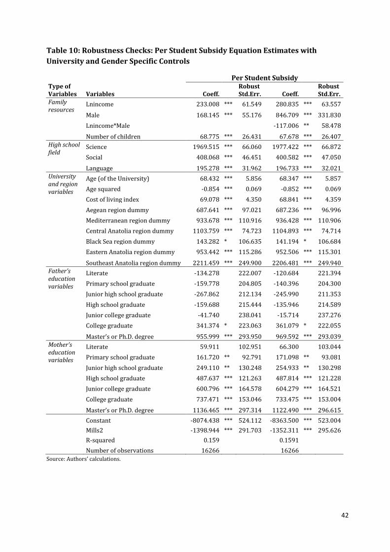
42

Table 10: Robustness Checks: Per Student Subsidy Equation Estimates with

University and Gender Specific Controls

Per Student Subsidy

Type of Variables Variables Coeff.

Robust Std.Err. Coeff.

Robust Std.Err.

Family resources

Lnincome 233.008 *** 61.549 280.835 *** 63.557

Male 168.145 *** 55.176 846.709 *** 331.830

Lnincome*Male

-117.006 ** 58.478

Number of children 68.775 *** 26.431 67.678 *** 26.407 High school field

Science 1969.515 *** 66.060 1977.422 *** 66.872

Social 408.068 *** 46.451 400.582 *** 47.050

Language 195.278 *** 31.962 196.733 *** 32.021 University and region variables

Age (of the University) 68.432 *** 5.856 68.347 *** 5.857

Age squared -0.854 *** 0.069 -0.852 *** 0.069

Cost of living index 69.078 *** 4.350 68.841 *** 4.359

Aegean region dummy 687.641 *** 97.021 687.236 *** 96.996

Mediterranean region dummy 933.678 *** 110.916 936.428 *** 110.906

Central Anatolia region dummy 1103.759 *** 74.723 1104.893 *** 74.714

Black Sea region dummy 143.282 * 106.635 141.194 * 106.684

Eastern Anatolia region dummy 953.442 *** 115.286 952.506 *** 115.301

Southeast Anatolia region dummy 2211.459 *** 249.900 2206.481 *** 249.940 Father’s education variables

Literate -134.278

222.007 -120.684

221.394

Primary school graduate -159.778

204.805 -140.396

204.300

Junior high school graduate -267.862

212.134 -245.990

211.353

High school graduate -159.688

215.444 -135.946

214.589

Junior college graduate -41.740

238.041 -15.714

237.276

College graduate 341.374 * 223.063 361.079 * 222.055

Master’s or Ph.D. degree 955.999 *** 293.950 969.592 *** 293.039 Mother’s education variables

Literate 59.911

102.951 66.300

103.044

Primary school graduate 161.720 ** 92.791 171.098 ** 93.081

Junior high school graduate 249.110 ** 130.248 254.933 ** 130.298

High school graduate 487.637 *** 121.263 487.814 *** 121.228

Junior college graduate 600.796 *** 164.578 604.279 *** 164.521

College graduate 737.471 *** 153.046 733.475 *** 153.004

Master’s or Ph.D. degree 1136.465 *** 297.314 1122.490 *** 296.615 Constant -8074.438 *** 524.112 -8363.500 *** 523.004 Mills2 -1398.944 *** 291.703 -1352.311 *** 295.626 R-squared 0.159

0.1591

Number of observations 16266

16266 Source: Authors’ calculations.

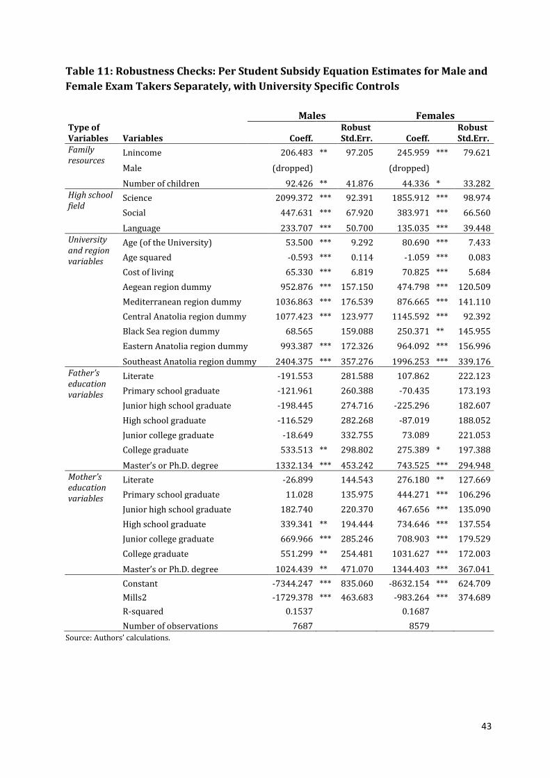
43

Table 11: Robustness Checks: Per Student Subsidy Equation Estimates for Male and

Female Exam Takers Separately, with University Specific Controls

Males Females

Type of Variables Variables Coeff.

Robust Std.Err. Coeff.

Robust Std.Err.

Family resources

Lnincome 206.483 ** 97.205 245.959 *** 79.621

Male (dropped)

(dropped)

Number of children 92.426 ** 41.876 44.336 * 33.282 High school field

Science 2099.372 *** 92.391 1855.912 *** 98.974

Social 447.631 *** 67.920 383.971 *** 66.560

Language 233.707 *** 50.700 135.035 *** 39.448 University and region variables

Age (of the University) 53.500 *** 9.292 80.690 *** 7.433

Age squared -0.593 *** 0.114 -1.059 *** 0.083

Cost of living 65.330 *** 6.819 70.825 *** 5.684

Aegean region dummy 952.876 *** 157.150 474.798 *** 120.509

Mediterranean region dummy 1036.863 *** 176.539 876.665 *** 141.110

Central Anatolia region dummy 1077.423 *** 123.977 1145.592 *** 92.392

Black Sea region dummy 68.565

159.088 250.371 ** 145.955

Eastern Anatolia region dummy 993.387 *** 172.326 964.092 *** 156.996

Southeast Anatolia region dummy 2404.375 *** 357.276 1996.253 *** 339.176 Father’s education variables

Literate -191.553

281.588 107.862

222.123

Primary school graduate -121.961

260.388 -70.435

173.193

Junior high school graduate -198.445

274.716 -225.296

182.607

High school graduate -116.529

282.268 -87.019

188.052

Junior college graduate -18.649

332.755 73.089

221.053

College graduate 533.513 ** 298.802 275.389 * 197.388

Master’s or Ph.D. degree 1332.134 *** 453.242 743.525 *** 294.948 Mother’s education variables

Literate -26.899

144.543 276.180 ** 127.669

Primary school graduate 11.028

135.975 444.271 *** 106.296

Junior high school graduate 182.740

220.370 467.656 *** 135.090

High school graduate 339.341 ** 194.444 734.646 *** 137.554

Junior college graduate 669.966 *** 285.246 708.903 *** 179.529

College graduate 551.299 ** 254.481 1031.627 *** 172.003

Master’s or Ph.D. degree 1024.439 ** 471.070 1344.403 *** 367.041 Constant -7344.247 *** 835.060 -8632.154 *** 624.709 Mills2 -1729.378 *** 463.683 -983.264 *** 374.689 R-squared 0.1537

0.1687

Number of observations 7687

8579 Source: Authors’ calculations.

44

7. Should students pay more for higher education?

In Turkey, the fees that public university students pay are very low and constitute a very

small portion of the total cost of education. In this section, we explore whether there is an

economic rationale for increasing tuition fees and hence the share of private

contributions in financing higher education. Some public university students come from

poor families, so they cannot afford to pay tuition. Assuming that we can deal with the

crucial issues of fairness and equal access to quality education by developing a well-

functioning system of financial aid, the answer to the question of whether the students’

share in financing the cost of higher education can be increased rests on whether there is

the ability and willingness to pay for higher education. To evaluate the ability and the

willingness to pay for higher education, we look at family income and how much families

actually pay for private tutoring and higher education.

In Table 12, Panel I, we show the mean and standard deviation of family income and

private tutoring expenditures for various sub-samples. Tutoring expenditures are

reported as the total spending during the student’s high school years, so we divide the

total amount by three to find the annual amount. However, based on our own

observations, we can say that most of the students attend private tutoring centers only in

their senior year in high school, therefore the values reported in the table are probably

underestimates of the true annual payments that parents make.

In panel II, we sort public university students by per student subsidy they receive

and report the mean and standard deviation of family income and tutoring expenditures

for various sub-groups. We present statistics for those who rank in the top 50 percent, top

25 percent and top 10 percent of the per student subsidy distribution. Although public

university students are poorer than private university students, those who receive a

higher subsidy from the government come from higher income families, again, consistent

with our earlier findings.

In Table 13, we present the highest and lowest fees in public and private

universities. In public universities, the highest fee is paid only by medical school and state

conservatory students. Most faculties charge fees in the range 230-330 TL. Comparing the

average income of public university students and especially the ones in the top 10%

group to the fees they pay, we can clearly see that the fees are too low. The fees that are

45

paid are lower than private tutoring spending, which is likely to be underestimated.

Therefore, clearly there is a gap between the willingness and ability to pay and the actual

payment for this group of students. Consistent with this finding, Figure 1 shows that many

public university students have family characteristics that are similar to those of private

university students. These findings suggest that public university fees can be increased, at

least in the universities with higher per student subsidy.

Table 12: Annual family income and private tutoring expenditures for various sub-

samples in the 2002 survey (in 2005 prices)

Variable: Family income Tutoring expenditure

Mean Stdev Mean Stdev

Panel I:

All (n=93266)

6846.47 6295.38 394.32 447.82

Success=1 (n=18464) 8846.50 8311.24 523.64 511.54

Success=0 (n=74802) 6352.79 5579.74 355.10 418.81

Public=1 (n=16251) 7703.71 6637.19 472.70 459.72

Public=0 (n=2213) 17238.51 13148.84 889.74 686.23

Panel II:

Per-student subsidy

Above median (n=8081) 8678.48 7331.90 517.35 501.40

Per-student subsidy

Top 25 percent (n=4098) 9337.92 7674.83 514.15 513.76

Per-student subsidy

Top 10 percent (n=1668) 10094.87 8020.36 510.80 541.71 Source: Author’s calculations.

46

Table 13: The highest and the lowest annual fees in public and private universities

(in 2005 TL)

Year 2000 2001 2002 2003 2004 2005

Public universities Lowest fee 181 209 157 150 148 147

Highest fee 559 781 486 468 461 456

Private universities Lowest fee 5103 8065 5151 3779 3114 4266

Highest fee 31893 47908 14258 21870 25655 26500

Source: Author’s calculations based on fee information from University Entrance Exam Application Booklets, various

years, OSYM. We exclude open university, where the fee was 55 TL.

8. Conclusions:

In this study, we investigate the university entrance outcomes of students with diverse

social and economic backgrounds using nationally representative data from Turkey. We

find that the children of families with higher income and education are more likely to

succeed in the highly competitive nationwide university entrance exam. Higher income

students are more likely to enter private universities rather than public universities.

However, among the students who are placed at public universities, those from families

with higher income and more education enter public universities that receive higher per-

student subsidies from the government.

We have data on per-student subsidy not only at a national level, but at the

university and faculty level as well. Our econometric analyses enable us to control for

possible selection problems and estimate the marginal effects of socio-economic

characteristics on subsidy received for public university entrants as well as for an average

exam taker.

Our results have important policy implications. When there is tough competition at

the university entrance, socio-economic background becomes an important determinant

of student success. Private universities can play an important role in providing higher

education to students that come from high income families and increase supply of tertiary

education. Within public university students, those from high income families seem to

have an advantage in getting into better funded universities. The fact that many of these

47

students have similar socio-economic characteristics with private university students

suggests that public university fees can and should be raised.

Acknowledgements:

We are grateful to Prof. Giray Berberoglu, Serkan Arikan and Dilara Bakan at OSYM for

providing us with the OSS data and answering our numerous questions. We are grateful to

Murside Canturk and Ahmet Kesik at the Ministry of Finance for their help with the

education finance data. We benefitted from helpful conversations with Sachi Hatakenaka

and Soner Baskaya. We thank Idil Bilgic Alpaslan, Hatice Calgan, Ibrahim Cicekli, Ekrem

Cunedioglu, Mert Can Duman, Veli Safak, and Firuzan Topaloglu for their help with

organizing the data. The usual disclaimer applies.

References:

Antoninis, Manos and Panos Tsakloglou (2001), “Who Benefits from Public Education in Greece?

Evidence and Policy Implications” Education Economics, 9:2, 197-222.

Atkinson, Anthony and Joseph Stiglitz (1980) Lectures on Public Economics (Maidenhead:

McGraw-Hill)

Barbaro, Salvatore (2005), Equity and Efficiency Considerations of Public Higher Education, Lecture

Notes in Economics and Mathematical systems, Vol.557, Springer Verlag.

Caner, Asena and Cagla Okten (2010), “Risk and career choice: Evidence from Turkey”, Economics

of Education Review, 29, 1060–1075.

Crean, John F. (1975), “The income redistributive effects of public spending on higher education”,

Journal of Human Resources, 10: 1 (Winter), 116 – 123.

Dow W.H. and Norton E.C. (2003) “Choosing Between and Interpreting the Heckit and Two-Part

Models for Corner Solutions”, Health Services & Outcomes Research Methodology, 4, 5-18.

Ebenstein, Avraham (2010) “The “Missing Girls” of China and the Unintended Consequences of the

One Child Policy”, Journal of Human Resources, Winter, 45 (1), 87-115.

Fernandez, Raquel and Richard Rogerson (1995). “On the political economy of education

subsidies”, Review of Economic Studies, 62, 249–262.

Ferreira, Francisco H. G., Jérémie Gignoux and Meltem Aran (2010) “Measuring Inequality of

Opportunity with Imperfect Data: The Case of Turkey”, Policy Research Working Paper 5204,

February, The World Bank.

48

Friedman, Milton., 1962. Capitalism and Freedom. The University of Chicago Press, Chicago.

Hansen, W. Lee and Burton A. Weisbrod (1969), “The Distribution of Costs and Direct Benefits of

Public Higher Education: The Case of California”, The Journal of Human Resources, 4: 2, (Spring),

176-191.

James, E., Benjamin, G., (1987), “Educational distribution and income redistribution

through education in Japan”, Journal of Human Resources 22: 4 (Autumn), 469 – 489.

Lemelin, Clement (1992), “Short-term redistributive effects of public financing of university

education in Quebec”, Canadian Public Policy - Analyse de Politiques, 18:2, 176 – 188.

Leung, S. F. and Yu, S. (1996). “On the choice between sample selection and two-part models”,

Journal of Econometrics, 72, 197–229.

Liu, Jin-Tan, Shin-Yi Chou, and Jin-Long Liu (2006), “Asymmetries in progression in higher

education in Taiwan: Parental education and income effects”, Economics of Education Review, 25,

647–658.

OECD (2010), Education at a Glance 2010: OECD Indicators, www.oecd.org/edu/eag2010 .

OSYM (Student Selection and Placement Center) (2005), Higher Education Statistics,

http://osym.gov.tr/belge/1-9467/2005-2006-ogretim-yili-yuksekogretim-istatistikleri-kit-.html.

Pechman, Joseph A. (1970), “The distributional effects of public higher education in California”,

The Journal of Human Resources, 5, 361 – 370.

Psacharopoulos, George, Jee-Peng Tan, and Emmanuel Jimenez (1986). Financing education in

developing countries: an exploration of policy options. Washington, DC: World Bank.

Roemer, John E. (1998): Equality of Opportunity. Cambridge, MA: Harvard University Press.

Rozada, Martin Gonzalez and Alicia Menendez (2002), “Public university in Argentina: subsidizing

the rich?”, Economics of Education Review, 21, 341–351.

Tansel, Aysit (2002) “Determinants of school attainment of boys and girls in Turkey: individual,

household and community factors”, Economics of Education Review, 21, 455–470.

Tansel Aysit and Fatma Bircan (2006), “Demand for education in Turkey: A Tobit analysis of

private tutoring expenditures”, Economics of Education Review, 25, 303-313.

Tuyluoglu Sevket, Ali Sait Albayrak (2010), “Hayat Pahalılığı ve Türkiye’de Illerin Hayat Pahalılığı

Sıralamasını Belirleyen En Önemli Faktörlerin Ridge Regresyon Analiziyle Incelenmesi (Cost of

Living and Examining with Ridge Regression Analysis the Most Important Factors that Determine

Cost of Living Ranking of Provinces in Turkey)”, Süleyman Demirel University, The Journal of

Faculty of Economics and Administrative Sciences, Vol.15, No.2, pp .63–91.

49

YOK (The Turkish Council of Higher Education) (2005), The Current State of Turkish Higher

Education, November, manuscript.

Appendix Table A1: The universities that offer the highest per student subsidy in

some majors.

Major: Economics

Major: Computer and Electronics Engineering

1 Orta Dogu Teknik 6922.98 1 Gebze Yuksek Tek Ens 17339.01 2 Galatasaray 5626.66 2 Izmir Yuksek Tek Ens 12508 3 Bogazici 5476.78 3 Orta Dogu Teknik 7884.41 4 Hacettepe 5313.35 4 Hacettepe 6970.42 5 Harran 4744.37 5 Bogazici 6469.54 6 Ankara 4361.66 6 İstanbul Teknik 5765.43 7 Yıldız Teknik 3034.62 7 Ankara 4470.21 8 Dokuz Eylul 3017.91 8 Dicle 4241.81 9 Ataturk 2683.53 9 Ege 3691.38 10 Ege 2622.76 10 Gaziantep 3535.54

Major: English Education

Major: Dentistry

1 Orta Dogu Teknik 6945.64 1 Dicle 14338.39 2 Hacettepe 4665.86 2 Hacettepe 13445.91 3 Bogazici 4497.91 3 Gazi 12548.09 4 Cukurova 2446.75 4 Ankara 11848.52 5 Ataturk 2420.62 5 Ataturk 10346.75 6 Inonu 2194.92 6 Ege 8810.26 7 Dicle 2170.31 7 İstanbul 8377.06 8 Kocaeli 2123.03 8 Ondokuz Mayıs 7813.38 9 Dokuz Eylul 2119.95 9 Cumhuriyet 7640.57 10 Uludag 2087.98 10 Suleyman Demirel 7244.59