Higher-Dimensional Algebra VI: Lie 2-Algebras

John C. BaezDepartment of Mathematics, University of California

Riverside, California 92521USA

Alissa S. CransDepartment of Mathematics, Loyola Marymount University

1 LMU Drive, Suite 2700Los Angeles, CA 90045

USA

email: baez@math.ucr.edu, acrans@lmu.edu

October 4, 2004

Abstract

The theory of Lie algebras can be categorified starting from a new notionof ‘2-vector space’, which we define as an internal category in Vect. Thereis a 2-category 2Vect having these 2-vector spaces as objects, ‘linear func-tors’ as morphisms and ‘linear natural transformations’ as 2-morphisms.We define a ‘semistrict Lie 2-algebra’ to be a 2-vector space L equippedwith a skew-symmetric bilinear functor [·, ·] : L × L → L satisfying theJacobi identity up to a completely antisymmetric trilinear natural trans-formation called the ‘Jacobiator’, which in turn must satisfy a certainlaw of its own. This law is closely related to the Zamolodchikov tetra-hedron equation, and indeed we prove that any semistrict Lie 2-algebragives a solution of this equation, just as any Lie algebra gives a solutionof the Yang–Baxter equation. We construct a 2-category of semistrict Lie2-algebras and prove that it is 2-equivalent to the 2-category of 2-termL∞-algebras in the sense of Stasheff. We also study strict and skeletalLie 2-algebras, obtaining the former from strict Lie 2-groups and usingthe latter to classify Lie 2-algebras in terms of 3rd cohomology classesin Lie algebra cohomology. This classification allows us to construct forany finite-dimensional Lie algebra g a canonical 1-parameter family of Lie2-algebras g~ which reduces to g at ~ = 0. These are closely related tothe 2-groups G~ constructed in a companion paper.

1

1 Introduction

One of the goals of higher-dimensional algebra is to ‘categorify’ mathematicalconcepts, replacing equational laws by isomorphisms satisfying new coherencelaws of their own. By iterating this process, we hope to find n-categorical andeventually ω-categorical generalizations of as many mathematical concepts aspossible, and use these to strengthen — and often simplify — the connectionsbetween different parts of mathematics. The previous paper of this series, HDA5[6], categorified the concept of Lie group and began to explore the resultingtheory of ‘Lie 2-groups’. Here we do the same for the concept of Lie algebra,obtaining a theory of ‘Lie 2-algebras’.

In the theory of groups, associativity plays a crucial role. When we categorifythe theory of groups, this equational law is replaced by an isomorphism calledthe associator, which satisfies a new law of its own called the pentagon equation.The counterpart of the associative law in the theory of Lie algebras is the Jacobiidentity. In a ‘Lie 2-algebra’ this is replaced by an isomorphism which we callthe Jacobiator. This isomorphism satisfies an interesting new law of its own.As we shall see, this law, like the pentagon equation, can be traced back toStasheff’s work on homotopy-invariant algebraic structures — in this case, hiswork on L∞-algebras, also known as strongly homotopy Lie algebras [24, 33].This demonstrates yet again the close connection between categorification andhomotopy theory.

To prepare for our work on Lie 2-algebras, we begin in Section 2 by review-ing the theory of internal categories. This gives a systematic way to categorifyconcepts: if K is some category of algebraic structures, a ‘category in K’ willbe one of these structures but with categories taking the role of sets. Unfor-tunately, this internalization process only gives a ‘strict’ way to categorify, inwhich equations are replaced by identity morphisms. Nonetheless it can be auseful first step.

In Section 3, we focus on categories in Vect, the category of vector spaces.We boldly call these ‘2-vector spaces’, despite the fact that this term is alreadyused to refer to a very different categorification of the concept of vector space[22], for it is our contention that our 2-vector spaces lead to a more interestingversion of categorified linear algebra than the traditional ones. For example,the tangent space at the identity of a Lie 2-group is a 2-vector space of oursort, and this gives a canonical representation of the Lie 2-group: its ‘adjointrepresentation’. This is contrast to the phenomenon observed by Barrett andMackaay [8], namely that Lie 2-groups have few interesting representations onthe traditional sort of 2-vector space. One reason for the difference is that thetraditional 2-vector spaces do not have a way to ‘subtract’ objects, while oursdo. This will be especially important for finding examples of Lie 2-algebras,since we often wish to set [x, y] = xy − yx.

At this point we should admit that our 2-vector spaces are far from novelentities! In fact, a category in Vect is secretly just the same as a 2-term chaincomplex of vector spaces. While the idea behind this correspondence goes backto Grothendieck [21], and is by now well-known to the cognoscenti, we describe

2

it carefully in Proposition 8, because it is crucial for relating ‘categorified linearalgebra’ to more familiar ideas from homological algebra.

In Section 4.1 we introduce the key concept of ‘semistrict Lie 2-algebra’.Roughly speaking, this is a 2-vector space L equipped with a bilinear functor

[·, ·] : L× L→ L,

the Lie bracket, that is skew-symmetric and satisfies the Jacobi identity up toa completely antisymmetric trilinear natural isomorphism, the ‘Jacobiator’ —which in turn is required to satisfy a law of its own, the ‘Jacobiator identity’.Since we do not weaken the equation [x, y] = −[y, x] to an isomorphism, we donot reach the more general concept of ‘weak Lie 2-algebra’: this remains a taskfor the future.

At first the Jacobiator identity may seem rather mysterious. As one mightexpect, it relates two ways of using the Jacobiator to rebracket an expression ofthe form [[[w, x], y], z], just as the pentagon equation relates two ways of usingthe associator to reparenthesize an expression of the form (((w ⊗ x) ⊗ y) ⊗ z).But its detailed form seems complicated and not particularly memorable.

However, it turns out that the Jacobiator identity is closely related to theZamolodchikov tetrahedron equation, familiar from the theory of 2-knots andbraided monoidal 2-categories [5, 7, 15, 16, 22]. In Section 4.2 we prove that justas any Lie algebra gives a solution of the Yang–Baxter equation, every semistrictLie 2-algebra gives a solution of the Zamolodchikov tetrahedron equation! Thispattern suggests that the theory of ‘Lie n-algebras’ — that is, structures likeLie algebras with (n − 1)-categories taking the role of sets — is deeply relatedto the theory of (n−1)-dimensional manifolds embedded in (n+1)-dimensionalspace.

In Section 4.3, we recall the definition of an L∞-algebra. Briefly, this isa chain complex V of vector spaces equipped with a bilinear skew-symmetricoperation [·, ·] : V × V → V which satisfies the Jacobi identity up to an infinitetower of chain homotopies. We construct a 2-category of ‘2-term’ L∞-algebras,that is, those with Vi = {0} except for i = 0, 1. Finally, we show this 2-categoryis equivalent to the previously defined 2-category of semistrict Lie 2-algebras.

In the next two sections we study strict and skeletal Lie 2-algebras, theformer being those where the Jacobi identity holds ‘on the nose’, while in thelatter, isomorphisms exist only between identical objects. Section 5 consists ofan introduction to strict Lie 2-algebras and strict Lie 2-groups, together withthe process for obtaining the strict Lie 2-algebra of a strict Lie 2-group. Section6 begins with an exposition of Lie algebra cohomology and its relationship toskeletal Lie 2-algebras. We then show that Lie 2-algebras can be classified (upto equivalence) in terms of a Lie algebra g, a representation of g on a vectorspace V , and an element of the Lie algebra cohomology group H3(g, V ). Withthe help of this result, we construct from any finite-dimensional Lie algebra g acanonical 1-parameter family of Lie 2-algebras g~ which reduces to g at ~ = 0.This is a new way of deforming a Lie algebra, in which the Jacobi identity isweakened in a manner that depends on the parameter ~. It is natural to suspect

3

that this deformation is related to the theory of quantum groups and affine Liealgebras. In HDA5, we give evidence for this by using Chern–Simons theoryto construct 2-groups G~ corresponding to the Lie 2-algebras g~ when ~ is aninteger. However, it would be nice to find a more direct link between quantumgroups, affine Lie algebras and the Lie 2-algebras g~.

In Section 7, we conclude with some guesses about how the work in thispaper should fit into a more general theory of ‘n-groups’ and ‘Lie n-algebras’.

Note: In all that follows, we denote the composite of morphisms f : x→ yand g : y → z as fg : x → z. All 2-categories and 2-functors referred to in thispaper are strict, though sometimes we include the word ‘strict’ to emphasizethis fact. We denote vertical composition of 2-morphisms by juxtaposition; wedenote horizontal composition and whiskering by the symbol ◦.

2 Internal Categories

In order to create a hybrid of the notions of a vector space and a category in thenext section, we need the concept of an ‘internal category’ within some category.The idea is that given a category K, we obtain the definition of a ‘category inK’ by expressing the definition of a usual (small) category completely in termsof commutative diagrams and then interpreting those diagrams within K. Thesame idea allows us to define functors and natural transformations in K, andultimately to recapitulate most of category theory, at least if K has propertiessufficiently resembling those of the category of sets.

Internal categories were introduced by Ehresmann [18] in the 1960s, and bynow they are a standard part of category theory [10]. However, since not allreaders may be familiar with them, for the sake of a self-contained treatmentwe start with the basic definitions.

Definition 1. Let K be a category. An internal category or category inK, say X, consists of:

• an object of objects X0 ∈ K,

• an object of morphisms X1 ∈ K,

together with

• source and target morphisms s, t : X1 → X0,

• a identity-assigning morphism i : X0 → X1,

• a composition morphism ◦ : X1 ×X0 X1 → X1

such that the following diagrams commute, expressing the usual category laws:

4

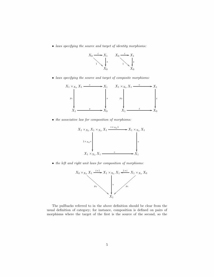
• laws specifying the source and target of identity morphisms:

X0i //

1 !!BBBBBBBB X1

s

��X0

X0i //

1 !!BBBBBBBB X1

t

��X0

• laws specifying the source and target of composite morphisms:

X1 ×X0 X1◦ //

p1

��

X1

s

��X1

s // X0

X1 ×X0 X1◦ //

p2

��

X1

t

��X1

t // X0

• the associative law for composition of morphisms:

X1 ×X0 X1 ×X0 X1

◦×X0 1//

1×X0◦

��

X1 ×X0 X1

◦

��X1 ×X0 X1

◦ // X1

• the left and right unit laws for composition of morphisms:

X0 ×X0 X1i×1 //

p2

!!CCCCCCCCCCCCCCCCCX1 ×X0 X1

◦

��

X1 ×X0 X01×ioo

p1

}}{{{{{{{{{{{{{{{{{

X1

The pullbacks referred to in the above definition should be clear from theusual definition of category; for instance, composition is defined on pairs ofmorphisms where the target of the first is the source of the second, so the

5

pullback X1 ×X0 X1 is defined via the square

X1 ×X0 X1p2 //

p1

��

X1

s

��X1

t // X0

Notice that inherent to this definition is the assumption that the pullbacksinvolved actually exist. This holds automatically when the ‘ambient category’Khas finite limits, but there are some important examples such as K = Diff wherethis is not the case. Throughout this paper, all of the categories considered havefinite limits:

• Set, the category whose objects are sets and whose morphisms are func-tions.

• Vect, the category whose objects are vector spaces over the field k andwhose morphisms are linear functions.

• Grp, the category whose objects are groups and whose morphisms are ho-momorphisms.

• Cat, the category whose objects are small categories and whose morphismsare functors.

• LieGrp, the category whose objects are Lie groups and whose morphismsare Lie group homomorphisms.

• LieAlg, the category whose objects are Lie algebras over the field k andwhose morphisms are Lie algebra homomorphisms.

Having defined ‘categories in K’, we can now internalize the notions offunctor and natural transformation in a similar manner. We shall use theseto construct a 2-category KCat consisting of categories, functors, and naturaltransformations in K.

Definition 2. Let K be a category. Given categories X and X ′ in K, aninternal functor or functor in K between them, say F : X → X ′, consists of:

• a morphism F0 : X0 → X ′0,

• a morphism F1 : X1 → X ′1

such that the following diagrams commute, corresponding to the usual laws sat-isfied by a functor:

6

• preservation of source and target:

X1s //

F1

��

X0

F0

��X ′1

s′ // X ′0

X1t //

F1

��

X0

F0

��X ′1

t′ // X ′0

• preservation of identity morphisms:

X0i //

F0

��

X1

F1

��X ′0

i′ // X ′1

• preservation of composite morphisms:

X1 ×X0 X1

F1×X0F1 //

◦

��

X ′1 ×X′0 X ′1

◦′

��X1

F1 // X ′1

Given two functors F : X → X ′ and G : X ′ → X ′′ in some category K, wedefine their composite FG : X → X ′′ by taking (FG)0 = F0G0 and (FG)1 =F1G1. Similarly, we define the identity functor in K, 1X : X → X , by taking(1X)0 = 1X0 and (1X)1 = 1X1 .

Definition 3. Let K be a category. Given two functors F,G : X → X ′ inK, an internal natural transformation or natural transformation inK between them, say θ : F ⇒ G, is a morphism θ : X0 → X ′1 for which thefollowing diagrams commute, expressing the usual laws satisfied by a naturaltransformation:

• laws specifying the source and target of a natural transformation:

X0θ //

F0 BBBBBBBB X ′1

s

��X0

X0θ //

G0 BBBBBBBB X ′1

t

��X0

7

• the commutative square law:

X1

∆(sθ×G) //

∆(F×tθ)

��

X ′1 ×X′0 X ′1

◦′

��X ′1 ×X′0 X ′1

◦′ // X ′1

Just like ordinary natural transformations, natural transformations in Kmay be composed in two different, but commuting, ways. First, let X and X ′

be categories in K and let F,G,H : X → X ′ be functors in K. If θ : F ⇒ G andτ : G⇒ H are natural transformations in K, we define their vertical composite,θτ : F ⇒ H, by

θτ := ∆(θ × τ) ◦′ .The reader can check that when K = Cat this reduces to the usual definitionof vertical composition. We can represent this composite pictorially as:

X

F

��

H

AAX′θτ

��

= X

F

��G //

H

AA

�

τ��

X ′

Next, letX,X ′, X ′′ be categories inK and let F,G : X → X ′ and F ′, G′ : X ′ →X ′′ be functors in K. If θ : F ⇒ G and θ′ : F ′ ⇒ G′ are natural transformationsin K, we define their horizontal composite, θ ◦ θ′ : FF ′ ⇒ GG′, in either oftwo equivalent ways:

θ ◦ θ′ := ∆(F0 × θ)(θ′ ×G′1) ◦′= ∆(θ ×G0)(F ′1 × θ′) ◦′ .

Again, this reduces to the usual definition when K = Cat. The horizontalcomposite can be depicted as:

X

FF ′

��

GG′

AAX′′θ◦θ′

��

= X

F

��

G

AAX′θ

��

F ′

��

G′

AAX′′θ′

��

It is routine to check that these composites are again natural transforma-tions in K. Finally, given a functor F : X → X ′ in K, the identity naturaltransformation 1F : F ⇒ F in K is given by 1F = F0i.

We now have all the ingredients of a 2-category:

8

Proposition 4. Let K be a category. Then there exists a strict 2-categoryKCat with categories in K as objects, functors in K as morphisms, and naturaltransformations in K as 2-morphisms, with composition and identities definedas above.

Proof. It is straightforward to check that all the axioms of a 2-category hold;this result goes back to Ehresmann [18]. ut

We now consider internal categories in Vect.

3 2-Vector spaces

Since our goal is to categorify the concept of a Lie algebra, we must first cat-egorify the concept of a vector space. A categorified vector space, or ‘2-vectorspace’, should be a category with structure analogous to that of a vector space,with functors replacing the usual vector space operations. Kapranov and Vo-evodsky [22] implemented this idea by taking a finite-dimensional 2-vector spaceto be a category of the form Vectn, in analogy to how every finite-dimensionalvector space is of the form kn. While this idea is useful in contexts such astopological field theory [25] and group representation theory [3], it has its lim-itations. As explained in the Introduction, these arise from the fact that these2-vector spaces have no functor playing the role of ‘subtraction’.

Here we instead define a 2-vector space to be a category in Vect. Just asthe main ingredient of a Lie algebra is a vector space, a Lie 2-algebra will havean underlying 2-vector space of this sort. Thus, in this section we first define a2-category of these 2-vector spaces. We then establish the relationship betweenthese 2-vector spaces and 2-term chain complexes of vector spaces: that is, chaincomplexes having only two nonzero vector spaces. We conclude this section bydeveloping some ‘categorified linear algebra’ — the bare minimum necessary fordefining and working with Lie 2-algebras in the next section.

In the following we consider vector spaces over an arbitrary field, k.

Definition 5. A 2-vector space is a category in Vect.

Thus, a 2-vector space V is a category with a vector space of objects V0

and a vector space of morphisms V1, such that the source and target mapss, t : V1 → V0, the identity-assigning map i : V0 → V1, and the composition map◦ : V1 ×V0 V1 → V1 are all linear. As usual, we write a morphism as f : x → ywhen s(f) = x and t(f) = y, and sometimes we write i(x) as 1x.

In fact, the structure of a 2-vector space is completely determined by thevector spaces V0 and V1 together with the source, target and identity-assigningmaps. As the following lemma demonstrates, composition can always be ex-pressed in terms of these, together with vector space addition:

Lemma 6. When K = Vect, one can omit all mention of composition in thedefinition of category in K, without any effect on the concept being defined.

9

Proof. First, given vector spaces V0, V1 and maps s, t : V1 → V0 and i : V0 →V1, we will define a composition operation that satisfies the laws in Definition1, obtaining a 2-vector space.

Given f ∈ V1, we define the arrow part of f, denoted as ~f , by

~f = f − i(s(f)).

Notice that ~f is in the kernel of the source map since

s(f − i(sf)) = s(f)− s(f) = 0.

While the source of ~f is always zero, its target may be computed as follows:

t(~f) = t(f − i(s(f)) = t(f)− s(f).

The meaning of the arrow part becomes clearer if we write f : x → y whens(f) = x and t(f) = y. Then, given any morphism f : x → y, we have ~f : 0 →y−x. In short, taking the arrow part of f has the effect of ‘translating f to theorigin’.

We can always recover any morphism from its arrow part together with itssource, since f = ~f + i(s(f)). We shall take advantage of this by identifying

f : x→ y with the ordered pair (x, ~f ). Note that with this notation we have

s(x, ~f) = x, t(x, ~f ) = x+ t(~f).

Using this notation, given morphisms f : x → y and g : y → z, we definetheir composite by

fg := (x, ~f + ~g),

or equivalently,(x, ~f)(y,~g) := (x, ~f + ~g).

It remains to show that with this composition, the diagrams of Definition 1 com-mute. The triangles specifying the source and target of the identity-assigningmorphism do not involve composition. The second pair of diagrams commutesince

s(fg) = x

andt(fg) = x+ t(~f) + t(~g) = x+ (y − x) + (z − y) = z.

The associative law holds for composition because vector space addition is as-sociative. Finally, the left unit law is satisfied since given f : x→ y,

i(x)f = (x, 0)(x, ~f ) = (x, ~f) = f

and similarly for the right unit law. We thus have a 2-vector space.Conversely, given a category V in Vect, we shall show that its composition

must be defined by the formula given above. Suppose that (f, g) = ((x, ~f ), (y,~g))

and (f ′, g′) = ((x′, ~f ′), (y′, ~g′)) are composable pairs of morphisms in V1. Since

10

the source and target maps are linear, (f + f ′, g + g′) also forms a composablepair, and the linearity of composition gives

(f + f ′)(g + g′) = fg + f ′g′.

If we set g = 1y and f ′ = 1y′ , the above equation becomes

(f + 1y′)(1y + g′) = f1y + 1y′g′ = f + g′.

Expanding out the left hand side we obtain

((x, ~f ) + (y′, 0))((y, 0) + (y′, ~g′)) = (x+ y′, ~f)(y + y′, ~g′),

while the right hand side becomes

(x, ~f ) + (y, ~g′) = (x+ y′, ~f + ~g′).

Thus we have (x+y′, ~f)(y+y′, ~g′) = (x+y′, ~f+~g′), so the formula for compositionin an arbitrary 2-vector space must be given by

fg = (x, ~f)(y,~g) = (x, ~f + ~g)

whenever (f, g) is a composable pair. This shows that we can leave out allreference to composition in the definition of ‘category in K’ without any effectwhen K = Vect. ut

In order to simplify future arguments, we will often use only the elements ofthe above lemma to describe a 2-vector space.

We continue by defining the morphisms between 2-vector spaces:

Definition 7. Given 2-vector spaces V and W , a linear functor F : V →Wis a functor in Vect from V to W .

For now we let 2Vect stand for the category of 2-vector spaces and linear functorsbetween them; later we will make 2Vect into a 2-category.

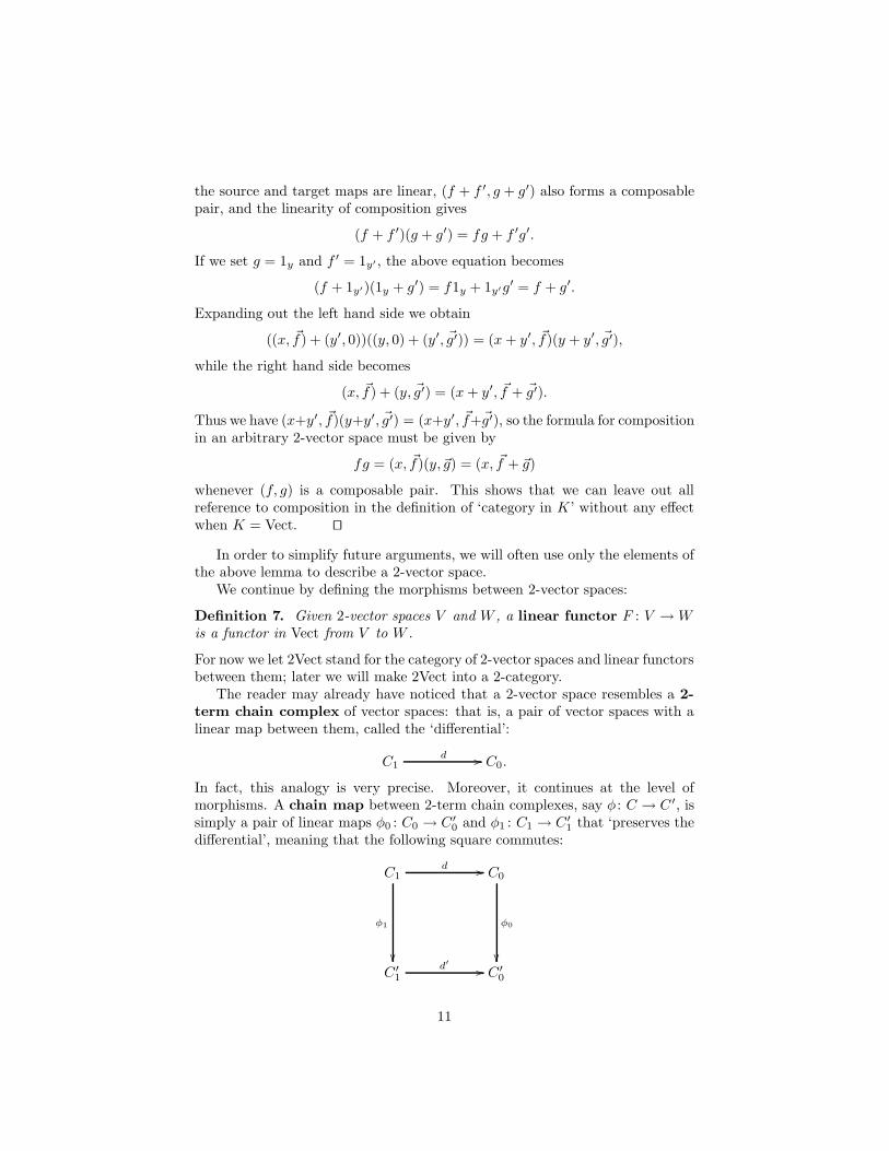
The reader may already have noticed that a 2-vector space resembles a 2-term chain complex of vector spaces: that is, a pair of vector spaces with alinear map between them, called the ‘differential’:

C1d // C0.

In fact, this analogy is very precise. Moreover, it continues at the level ofmorphisms. A chain map between 2-term chain complexes, say φ : C → C ′, issimply a pair of linear maps φ0 : C0 → C ′0 and φ1 : C1 → C ′1 that ‘preserves thedifferential’, meaning that the following square commutes:

C1d //

φ1

��

C0

φ0

��C ′1

d′ // C ′0

11

There is a category 2Term whose objects are 2-term chain complexes and whosemorphisms are chain maps. Moreover:

Proposition 8. The categories 2Vect and 2Term are equivalent.

Proof. We begin by introducing functors

S : 2Vect→ 2Term

andT : 2Term→ 2Vect.

We first define S. Given a 2-vector space V , we define S(V ) = C where C isthe 2-term chain complex with

C0 = V0,

C1 = ker(s) ⊆ V1,

d = t|C1 ,

and s, t : V1 → V0 are the source and target maps associated with the 2-vectorspace V . It remains to define S on morphisms. Let F : V → V ′ be a linearfunctor and let S(V ) = C, S(V ′) = C ′. We define S(F ) = φ where φ is thechain map with φ0 = F0 and φ1 = F1|C1 . Note that φ preserves the differentialbecause F preserves the target map.

We now turn to the second functor, T . Given a 2-term chain complex C, wedefine T (C) = V where V is a 2-vector space with

V0 = C0,

V1 = C0 ⊕ C1.

To completely specify V it suffices by Lemma 6 to specify linear maps s, t : V1 →V0 and i : V0 → V1 and check that s(i(x)) = t(i(x)) = x for all x ∈ V0. To define

s and t, we write any element f ∈ V1 as a pair (x, ~f) ∈ C0 ⊕ C1 and set

s(f) = s(x, ~f) = x,

t(f) = t(x, ~f) = x+ d~f.

For i, we use the same notation and set

i(x) = (x, 0)

for all x ∈ V0. Clearly s(i(x)) = t(i(x)) = x. Note also that with thesedefinitions, the decomposition V1 = C0 ⊕ C1 is precisely the decompositionof morphisms into their source and ‘arrow part’, as in the proof of Lemma 6.Moreover, given any morphism f = (x, ~f) ∈ V1, we have

t(f)− s(f) = d~f.

12

Next we define T on morphisms. Suppose φ : C → C ′ is a chain map between2-term chain complexes:

C1d //

φ1

��

C0

φ0

��C ′1

d′ // C ′0

Let T (C) = V and T (C ′) = V ′. Then we define F = T (φ) where F : V → V ′

is the linear functor with F0 = φ0 and F1 = φ0 ⊕ φ1. To check that F reallyis a linear functor, note that it is linear on objects and morphisms. Moreover,it preserves the source and target, identity-assigning and composition mapsbecause all these are defined in terms of addition and the differential in thechain complexes C and C ′, and φ is linear and preserves the differential.

We leave it the reader to verify that T and S are indeed functors. Toshow that S and T form an equivalence, we construct natural isomorphismsα : ST ⇒ 12Vect and β : TS ⇒ 12Term.

To construct α, consider a 2-vector space V . Applying S to V we obtain the2-term chain complex

ker(s)t|ker(s) // V0.

Applying T to this result, we obtain a 2-vector space V ′ with the space V0 ofobjects and the space V0⊕ker(s) of morphisms. The source map for this 2-vector

space is given by s′(x, ~f) = x, the target map is given by t′(x, ~f) = x + t(~f),and the identity-assigning map is given by i′(x) = (x, 0). We thus can define anisomorphism αV : V ′ → V by setting

(αV )0(x) = x,

(αV )1(x, ~f) = i(x) + ~f.

It is easy to check that αV is a linear functor. It is an isomorphism thanks tothe fact, shown in the proof of Lemma 6, that every morphism in V can beuniquely written as i(x) + ~f where x is an object and ~f ∈ ker(s).

To construct β, consider a 2-term chain complex, C, given by

C1d // C0.

Then T (C) is the 2-vector space with the space C0 of objects, the space C0⊕C1 of

morphisms, together with the source and target maps s : (x, ~f) 7→ x, t : (x, ~f ) 7→x+ d~f and the identity-assigning map i : x 7→ (x, 0). Applying the functor S tothis 2-vector space we obtain a 2-term chain complex C ′ given by:

ker(s)t|ker(s) // C0.

13

Since ker(s) = {(x, ~f)|x = 0} ⊆ C0 ⊕ C1, there is an obvious isomorphismker(s) ∼= C1. Using this we obtain an isomorphism βC : C ′ → C given by:

ker(s)t|ker(s) //

∼

��

C0

1

��C1

d // C0

where the square commutes because of how we have defined t.We leave it to the reader to verify that α and β are indeed natural isomor-

phisms. ut

As mentioned in the Introduction, the idea behind Proposition 8 goes back atleast to Grothendieck [21], who showed that groupoids in the category of abeliangroups are equivalent to 2-term chain complexes of abelian groups. There aremany elaborations of this idea, some of which we will mention later, but for nowthe only one we really need involves making 2Vect and 2Term into 2-categoriesand showing that they are 2-equivalent as 2-categories. To do this, we requirethe notion of a ‘linear natural transformation’ between linear functors. Thiswill correspond to a chain homotopy between chain maps.

Definition 9. Given two linear functors F,G : V → W between 2-vector spaces,a linear natural transformation α : F ⇒ G is a natural transformation inVect.

Definition 10. We define 2Vect to be VectCat, or in other words, the 2-category of 2-vector spaces, linear functors and linear natural transformations.

Recall that in general, given two chain maps φ, ψ : C → C ′, a chain homo-topy τ : φ ⇒ ψ is a family of linear maps τ : Cp → C ′p+1 such that τpd

′p+1 +

dpτp−1 = ψp−φp for all p. In the case of 2-term chain complexes, a chain homo-topy amounts to a map τ : C0 → C ′1 satisfying τd′ = ψ0−φ0 and dτ = ψ1−φ1.

Definition 11. We define 2Term to be the 2-category of 2-term chain com-plexes, chain maps, and chain homotopies.

We will continue to sometimes use 2Term and 2Vect to stand for the underlyingcategories of these (strict) 2-categories. It will be clear by context whether wemean the category or the 2-category.

The next result strengthens Proposition 8.

Theorem 12. The 2-category 2Vect is 2-equivalent to the 2-category 2Term.

14

Proof. We begin by constructing 2-functors

S : 2Vect→ 2Term

andT : 2Term→ 2Vect.

By Proposition 8, we need only to define S and T on 2-morphisms. Let V and V ′

be 2-vector spaces, F,G : V → V ′ linear functors, and θ : F ⇒ G a linear naturaltransformation. Then we define the chain homotopy S(θ) : S(F )⇒ S(G) by

S(θ)(x) = ~θx,

using the fact that a 0-chain x of S(V ) is the same as an object x of V . Con-versely, let C and C ′ be 2-term chain complexes, φ, ψ : C → C ′ chain maps andτ : φ ⇒ ψ a chain homotopy. Then we define the linear natural transformationT (τ) : T (φ)⇒ T (ψ) by

T (τ)(x) = (φ0(x), τ(x)),

where we use the description of a morphism in S(C ′) as a pair consisting of itssource and its arrow part, which is a 1-chain in C ′. We leave it to the reader tocheck that S is really a chain homotopy, T is really a linear natural transforma-tion, and that the natural isomorphisms α : ST ⇒ 12Vect and β : TS ⇒ 12Term

defined in the proof of Proposition 8 extend to this 2-categorical context. ut

We conclude this section with a little categorified linear algebra. We considerthe direct sum and tensor product of 2-vector spaces.

Proposition 13. Given 2-vector spaces V = (V0, V1, s, t, i, ◦) and V ′ = (V ′0 , V′

1 ,s′, t′, i′, ◦′), there is a 2-vector space V ⊕ V ′ having:

• V0 ⊕ V ′0 as its vector space of objects,

• V1 ⊕ V ′1 as its vector space of morphisms,

• s⊕ s′ as its source map,

• t⊕ t′ as its target map,

• i⊕ i′ as its identity-assigning map, and

• ◦ ⊕ ◦′ as its composition map.

Proof. The proof amounts to a routine verification that the diagrams inDefinition 1 commute. ut

Proposition 14. Given 2-vector spaces V = (V0, V1, s, t, i, ◦) and V ′ = (V ′0 , V′

1 ,s′, t′, i′, ◦′), there is a 2-vector space V ⊗ V ′ having:

• V0 ⊗ V ′0 as its vector space of objects,

15

• V1 ⊗ V ′1 as its vector space of morphisms,

• s⊗ s′ as its source map,

• t⊗ t′ as its target map,

• i⊗ i′ as its identity-assigning map, and

• ◦ ⊗ ◦′ as its composition map.

Proof. Again, the proof is a routine verification. ut

We now check the correctness of the above definitions by showing the uni-versal properties of the direct sum and tensor product. These universal prop-erties only require the category structure of 2Vect, not its 2-category structure,since the necessary diagrams commute ‘on the nose’ rather than merely up to a2-isomorphism, and uniqueness holds up to isomorphism, not just up to equiv-alence. The direct sum is what category theorists call a ‘biproduct’: both aproduct and coproduct, in a compatible way [26]:

Proposition 15. The direct sum V ⊕V ′ is the biproduct of the 2-vector spacesV and V ′, with the obvious inclusions

i : V → V ⊕ V ′, i′ : V ′ → V ⊕ V ′

and projectionsp : V ⊕ V ′ → V, p′ : V ⊕ V ′ → V ′.

Proof. A routine verification. ut

Since the direct sum V ⊕ V ′ is a product in the categorical sense, we mayalso denote it by V × V ′, as we do now in defining a ‘bilinear functor’, which isused in stating the universal property of the tensor product:

Definition 16. Let V, V ′, and W be 2-vector spaces. A bilinear functorF : V × V ′ →W is a functor such that the underlying map on objects

F0 : V0 × V ′0 → W0

and the underlying map on morphisms

F1 : V1 × V ′1 → W1

are bilinear.

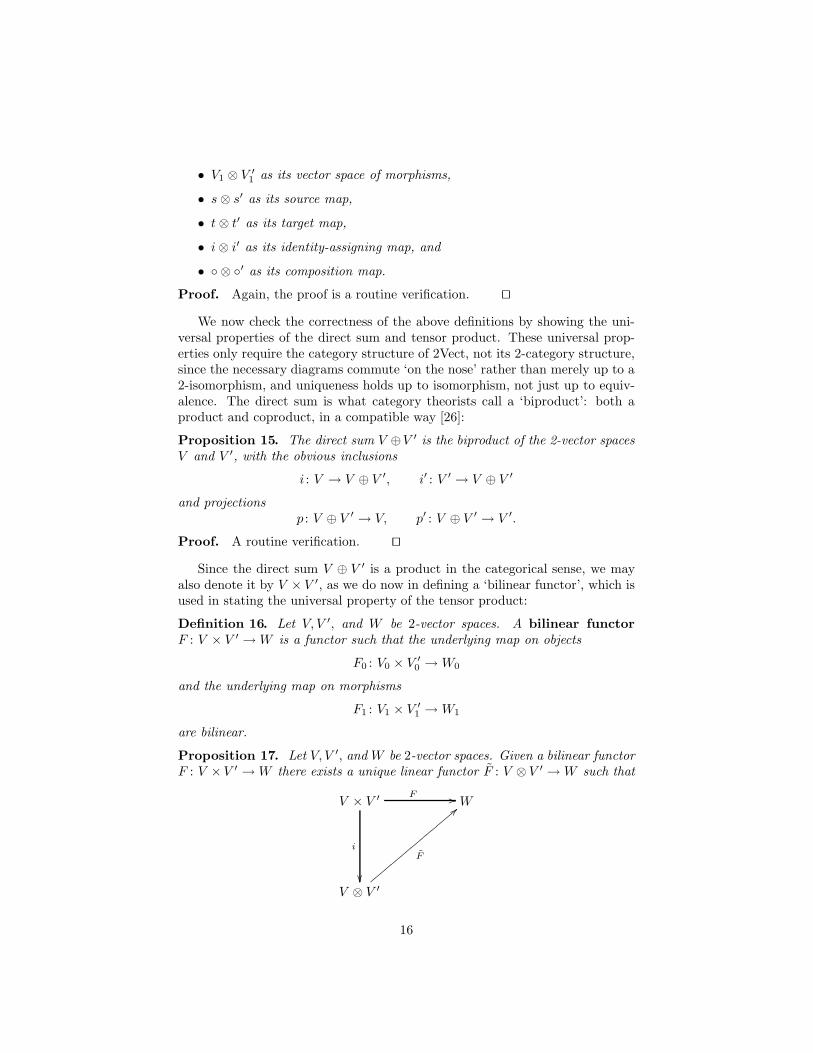
Proposition 17. Let V, V ′, and W be 2-vector spaces. Given a bilinear functorF : V ×V ′ →W there exists a unique linear functor F : V ⊗ V ′ → W such that

V × V ′ F //

i

��

W

V ⊗ V ′

F

==zzzzzzzzzzzzzzzzz

16

commutes, where i : V × V ′ → V ⊗ V ′ is given by (v, w) 7→ v ⊗ w for (v, w) ∈(V × V ′)0 and (f, g) 7→ f ⊗ g for (f, g) ∈ (V × V ′)1.

Proof. The existence and uniqueness of F0 : (V ⊗ V ′)0 → W0 andF1 : (V ⊗ V ′)1 → W1 follow from the universal property of the tensor prod-uct of vector spaces, and it is then straightforward to check that F is a linearfunctor. ut

We can also form the tensor product of linear functors. Given linear functorsF : V → V ′ and G : W →W ′, we define F ⊗G : V ⊗ V ′ →W ⊗W ′ by setting:

(F ⊗G)0 = F0 ⊗G0,(F ⊗G)1 = F1 ⊗G1.

Furthermore, there is an ‘identity object’ for the tensor product of 2-vectorspaces. In Vect, the ground field k acts as the identity for tensor product: thereare canonical isomorphisms k ⊗ V ∼= V and V ⊗ k ∼= V . For 2-vector spaces, acategorified version of the ground field plays this role:

Proposition 18. There exists a unique 2-vector space K, the categorifiedground field, with K0 = K1 = k and s, t, i = 1k.

Proof. Lemma 6 implies that there is a unique way to define composition inK making it into a 2-vector space. In fact, every morphism in K is an identitymorphism. utProposition 19. Given any 2-vector space V , there is an isomorphism `V : K⊗V → V , which is defined on objects by a ⊗ v 7→ av and on morphisms bya⊗ f 7→ af . There is also an isomorphism rV : V ⊗K → V , defined similarly.

Proof. This is straightforward. ut

The functors `V and rV are a categorified version of left and right multiplica-tion by scalars. Our 2-vector spaces also have a categorified version of addition,namely a linear functor

+: V ⊕ V → V

mapping any pair (x, y) of objects or morphisms to x+ y. Combining this withscalar multiplication by the object −1 ∈ K, we obtain another linear functor

− : V ⊕ V → V

mapping (x, y) to x − y. This is the sense in which our 2-vector spaces areequipped with a categorified version of subtraction. All the usual rules governingaddition of vectors, subtraction of vectors, and scalar multiplication hold ‘on thenose’ as equations.

One can show that with the above tensor product, the category 2Vect be-comes a symmetric monoidal category. One can go further and make the 2-category version of 2Vect into a symmetric monoidal 2-category [17], but wewill not need this here. Now that we have a definition of 2-vector space andsome basic tools of categorified linear algebra we may proceed to the main focusof this paper: the definition of a categorified Lie algebra.

17

4 Semistrict Lie 2-algebras

4.1 Definitions

We now introduce the concept of a ‘Lie 2-algebra’, which blends together thenotion of a Lie algebra with that of a category. As mentioned previously, toobtain a Lie 2-algebra we begin with a 2-vector space and equip it with a bracketfunctor, which satisfies the Jacobi identity up to a natural isomorphism, the‘Jacobiator’. Then we require that the Jacobiator satisfy a new coherence lawof its own, the ‘Jacobiator identity’. We shall assume the bracket is bilinear inthe sense of Definition 16, and also skew-symmetric:

Definition 20. Let V and W be 2-vector spaces. A bilinear functor F : V ×V →W is skew-symmetric if F (x, y) = −F (y, x) whenever (x, y) is an objector morphism of V × V . If this is the case we also say the corresponding linearfunctor F : V ⊗ V →W is skew-symmetric.

We shall also assume that the Jacobiator is trilinear and completely antisym-metric:

Definition 21. Let V and W be 2-vector spaces. A functor F : V n → W isn-linear if F (x1, . . . , xn) is linear in each argument, where (x1, . . . , xn) is anobject or morphism of V n. Given n-linear functors F,G : V n → W , a naturaltransformation θ : F ⇒ G is n-linear if θx1,...,xn depends linearly on each objectxi, and completely antisymmetric if the arrow part of θx1,...,xn is completelyantisymmetric under permutations of the objects.

Since we do not weaken the bilinearity or skew-symmetry of the bracket, we callthe resulting sort of Lie 2-algebra ‘semistrict’:

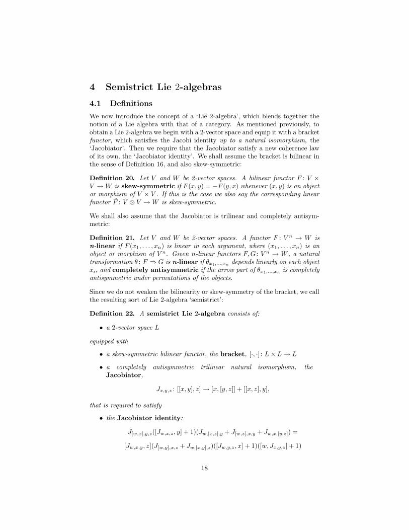
Definition 22. A semistrict Lie 2-algebra consists of:

• a 2-vector space L

equipped with

• a skew-symmetric bilinear functor, the bracket, [·, ·] : L× L→ L

• a completely antisymmetric trilinear natural isomorphism, theJacobiator,

Jx,y,z : [[x, y], z]→ [x, [y, z]] + [[x, z], y],

that is required to satisfy

• the Jacobiator identity:

J[w,x],y,z([Jw,x,z, y] + 1)(Jw,[x,z],y + J[w,z],x,y + Jw,x,[y,z]) =

[Jw,x,y, z](J[w,y],x,z + Jw,[x,y],z)([Jw,y,z, x] + 1)([w, Jx,y,z] + 1)

18

for all w, x, y, z ∈ L0. (There is only one choice of identity morphism that canbe added to each term to make the composite well-defined.)

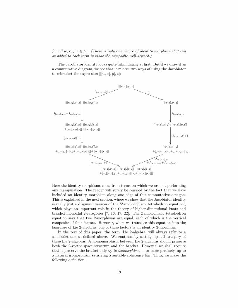
The Jacobiator identity looks quite intimidating at first. But if we draw it asa commutative diagram, we see that it relates two ways of using the Jacobiatorto rebracket the expression [[[w, x], y], z]:

[[[w,x],y],z]

[[[w,y],x],z]+[[w,[x,y]],z] [[[w,x],y],z]

[[[w,y],z],x]+[[w,y],[x,z]]

+[w,[[x,y],z]]+[[w,z],[x,y]]

[[[w,x],z],y]+[[w,x],[y,z]]

[[[w,z],y],x]+[[w,[y,z]],x]

+[[w,y],[x,z]]+[w,[[x,y],z]]+[[w,z],[x,y]]

[[w,[x,z]],y]

+[[w,x],[y,z]]+[[[w,z],x],y]

[[[w,z],y],x]+[[w,z],[x,y]]+[[w,y],[x,z]]

+[w,[[x,z],y]]+[[w,[y,z]],x]+[w,[x,[y,z]]]

Jw,[x,z],y

+J[w,z],x,y+Jw,x,[y,z]

[Jw,x,y,z]

uukkkkkkkkkkkkkkkkk1

))SSSSSSSSSSSSSSSSS

J[w,y],x,z+Jw,[x,y],z

��

[Jw,y,z ,x]+1

��

J[w,x],y,z

��

[Jw,x,z,y]+1

��

[w,Jx,y,z]+1))RRRRRRRRRRRRRRRRRR

uullllllllllllllllll

Here the identity morphisms come from terms on which we are not performingany manipulation. The reader will surely be puzzled by the fact that we haveincluded an identity morphism along one edge of this commutative octagon.This is explained in the next section, where we show that the Jacobiator identityis really just a disguised version of the ‘Zamolodchikov tetrahedron equation’,which plays an important role in the theory of higher-dimensional knots andbraided monoidal 2-categories [7, 16, 17, 22]. The Zamolochikov tetrahedronequation says that two 2-morphisms are equal, each of which is the verticalcomposite of four factors. However, when we translate this equation into thelanguage of Lie 2-algebras, one of these factors is an identity 2-morphism.

In the rest of this paper, the term ‘Lie 2-algebra’ will always refer to asemistrict one as defined above. We continue by setting up a 2-category ofthese Lie 2-algebras. A homomorphism between Lie 2-algebras should preserveboth the 2-vector space structure and the bracket. However, we shall requirethat it preserve the bracket only up to isomorphism — or more precisely, up toa natural isomorphism satisfying a suitable coherence law. Thus, we make thefollowing definition.

19

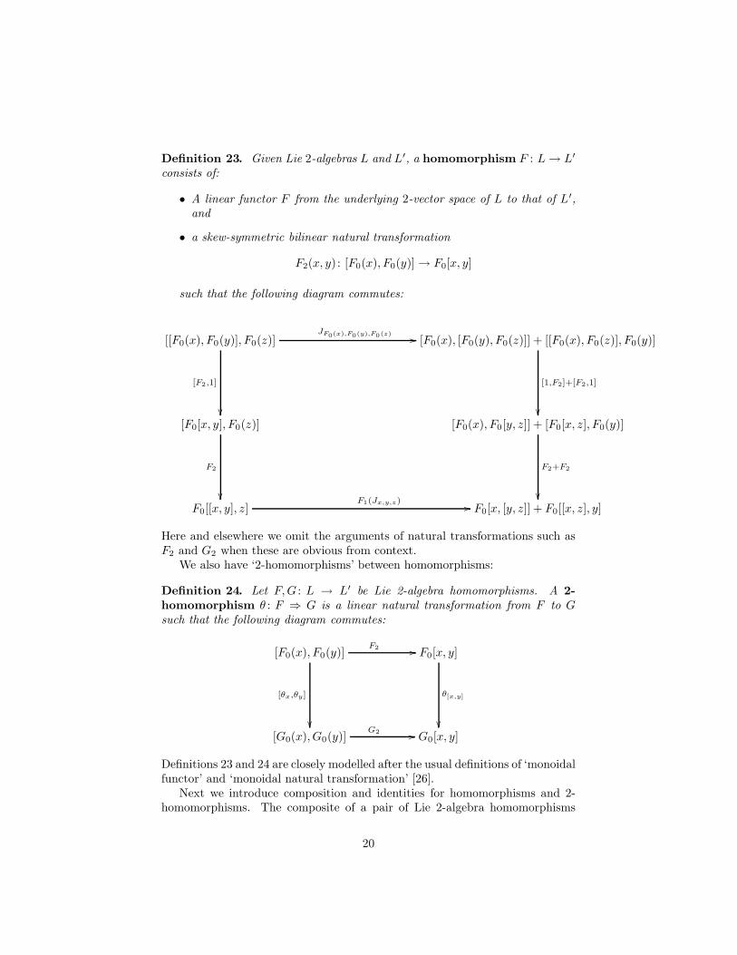
Definition 23. Given Lie 2-algebras L and L′, a homomorphism F : L→ L′

consists of:

• A linear functor F from the underlying 2-vector space of L to that of L′,and

• a skew-symmetric bilinear natural transformation

F2(x, y) : [F0(x), F0(y)]→ F0[x, y]

such that the following diagram commutes:

[[F0(x), F0(y)], F0(z)]JF0(x),F0(y),F0(z) //

[F2,1]

��

[F0(x), [F0(y), F0(z)]] + [[F0(x), F0(z)], F0(y)]

[1,F2]+[F2,1]

��[F0[x, y], F0(z)]

F2

��

[F0(x), F0[y, z]] + [F0[x, z], F0(y)]

F2+F2

��F0[[x, y], z]

F1(Jx,y,z) // F0[x, [y, z]] + F0[[x, z], y]

Here and elsewhere we omit the arguments of natural transformations such asF2 and G2 when these are obvious from context.

We also have ‘2-homomorphisms’ between homomorphisms:

Definition 24. Let F,G : L → L′ be Lie 2-algebra homomorphisms. A 2-homomorphism θ : F ⇒ G is a linear natural transformation from F to Gsuch that the following diagram commutes:

[F0(x), F0(y)]F2 //

[θx,θy]

��

F0[x, y]

θ[x,y]

��[G0(x), G0(y)]

G2 // G0[x, y]

Definitions 23 and 24 are closely modelled after the usual definitions of ‘monoidalfunctor’ and ‘monoidal natural transformation’ [26].

Next we introduce composition and identities for homomorphisms and 2-homomorphisms. The composite of a pair of Lie 2-algebra homomorphisms

20

F : L→ L′ and G : L′ → L′′ is given by letting the functor FG : L→ L′′ be theusual composite of F and G:

LF // L′

G // L′′

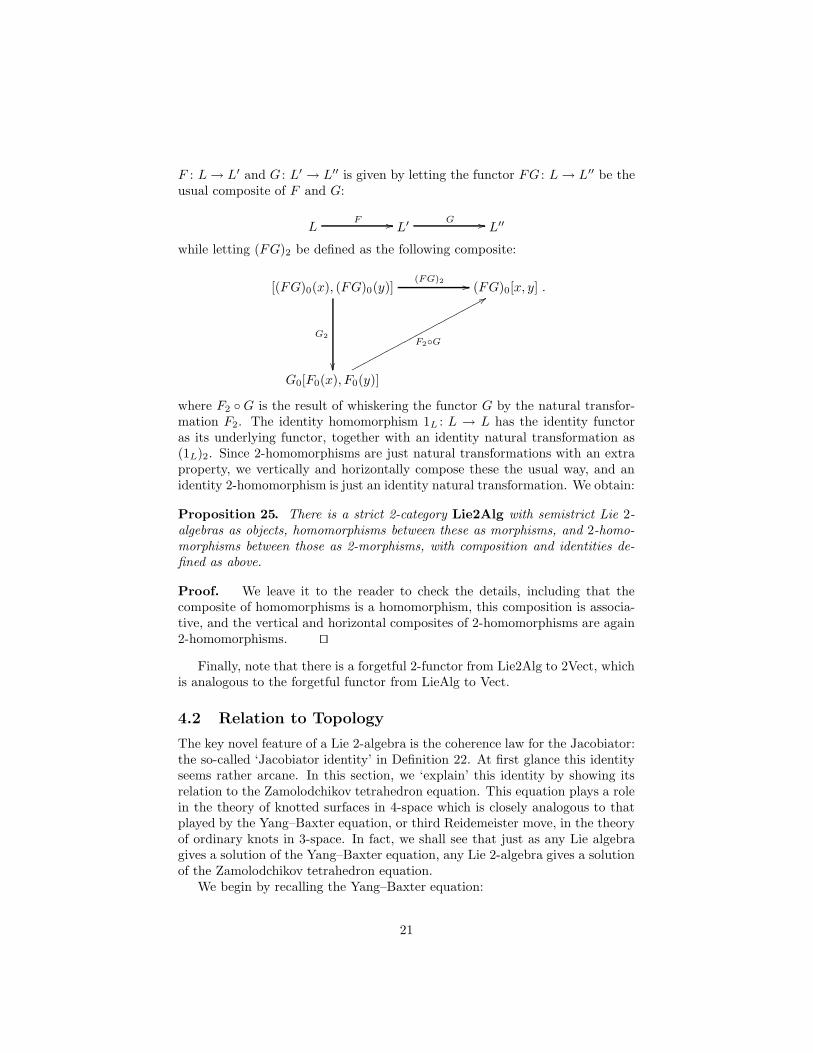
while letting (FG)2 be defined as the following composite:

[(FG)0(x), (FG)0(y)](FG)2 //

G2

��

(FG)0[x, y]

G0[F0(x), F0(y)]

F2◦G

88ppppppppppppppppppppppp

.

where F2 ◦G is the result of whiskering the functor G by the natural transfor-mation F2. The identity homomorphism 1L : L → L has the identity functoras its underlying functor, together with an identity natural transformation as(1L)2. Since 2-homomorphisms are just natural transformations with an extraproperty, we vertically and horizontally compose these the usual way, and anidentity 2-homomorphism is just an identity natural transformation. We obtain:

Proposition 25. There is a strict 2-category Lie2Alg with semistrict Lie 2-algebras as objects, homomorphisms between these as morphisms, and 2-homo-morphisms between those as 2-morphisms, with composition and identities de-fined as above.

Proof. We leave it to the reader to check the details, including that thecomposite of homomorphisms is a homomorphism, this composition is associa-tive, and the vertical and horizontal composites of 2-homomorphisms are again2-homomorphisms. ut

Finally, note that there is a forgetful 2-functor from Lie2Alg to 2Vect, whichis analogous to the forgetful functor from LieAlg to Vect.

4.2 Relation to Topology

The key novel feature of a Lie 2-algebra is the coherence law for the Jacobiator:the so-called ‘Jacobiator identity’ in Definition 22. At first glance this identityseems rather arcane. In this section, we ‘explain’ this identity by showing itsrelation to the Zamolodchikov tetrahedron equation. This equation plays a rolein the theory of knotted surfaces in 4-space which is closely analogous to thatplayed by the Yang–Baxter equation, or third Reidemeister move, in the theoryof ordinary knots in 3-space. In fact, we shall see that just as any Lie algebragives a solution of the Yang–Baxter equation, any Lie 2-algebra gives a solutionof the Zamolodchikov tetrahedron equation.

We begin by recalling the Yang–Baxter equation:

21

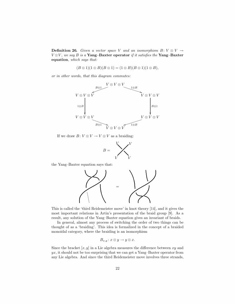
Definition 26. Given a vector space V and an isomorphism B : V ⊗ V →V ⊗V , we say B is a Yang–Baxter operator if it satisfies the Yang–Baxterequation, which says that:

(B ⊗ 1)(1⊗B)(B ⊗ 1) = (1⊗B)(B ⊗ 1)(1⊗B),

or in other words, that this diagram commutes:

V ⊗ V ⊗ V

V ⊗ V ⊗ V

V ⊗ V ⊗ V

V ⊗ V ⊗ V

V ⊗ V ⊗ V

V ⊗ V ⊗ V

1⊗B**UUUUUUUUUU

B⊗1

uujjjjjjjjj

1⊗B

��

B⊗1 ))TTTTTTTTT

1⊗Bttiiiiiiiiii

B⊗1

��

If we draw B : V ⊗ V → V ⊗ V as a braiding:

V V

B =

V V

the Yang–Baxter equation says that:

%%%%%%=

This is called the ‘third Reidemeister move’ in knot theory [14], and it gives themost important relations in Artin’s presentation of the braid group [9]. As aresult, any solution of the Yang–Baxter equation gives an invariant of braids.

In general, almost any process of switching the order of two things can bethought of as a ‘braiding’. This idea is formalized in the concept of a braidedmonoidal category, where the braiding is an isomorphism

Bx,y : x⊗ y → y ⊗ x.

Since the bracket [x, y] in a Lie algebra measures the difference between xy andyx, it should not be too surprising that we can get a Yang–Baxter operator fromany Lie algebra. And since the third Reidemeister move involves three strands,

22

while the Jacobi identity involves three Lie algebra elements, it should also notbe surprising that the Yang–Baxter equation is actually equivalent to the Jacobiidentity in a suitable context:

Proposition 27. Let L be a vector space equipped with a skew-symmetric bi-linear operation [·, ·] : L × L → L. Let L′ = k ⊕ L and define the isomorphismB : L′ ⊗ L′ → L′ ⊗ L′ by

B((a, x)⊗ (b, y)) = (b, y)⊗ (a, x) + (1, 0)⊗ (0, [x, y]).

Then B is a solution of the Yang–Baxter equation if and only if [·, ·] satisfiesthe Jacobi identity.

Proof. The proof is a calculation best left to the reader. ut

The nice thing is that this result has a higher-dimensional analogue, obtainedby categorifying everything in sight! The analogue of the Yang–Baxter equationis called the ‘Zamolodchikov tetrahedron equation’:

Definition 28. Given a 2-vector space V and an invertible linear functor B : V⊗V → V ⊗ V , a linear natural isomorphism

Y : (B ⊗ 1)(1⊗B)(B ⊗ 1)⇒ (1⊗B)(B ⊗ 1)(1⊗B)

satisfies the Zamolodchikov tetrahedron equation if

[(Y ⊗1)◦(1⊗1⊗B)(1⊗B⊗1)(B⊗1⊗1)][(1⊗B⊗1)(B⊗1⊗1)◦(1⊗Y )◦(B⊗1⊗1)]

[(1⊗B⊗1)(1⊗1⊗B)◦(Y ⊗1)◦(1⊗1⊗B)][(1⊗Y )◦(B⊗1⊗1)(1⊗B⊗1)(1⊗1⊗B)]

=

[(B⊗1⊗1)(1⊗B⊗1)(1⊗1⊗B)◦(Y ⊗1)][(B⊗1⊗1)◦(1⊗Y )◦(B⊗1⊗1)(1⊗B⊗1)]

[(1⊗1⊗B)◦(Y⊗1)◦(1⊗1⊗B)(1⊗B⊗1)][(1⊗1⊗B)(1⊗B⊗1)(B⊗1⊗1)◦(1⊗Y )],

where ◦ represents the whiskering of a linear functor by a linear natural trans-formation.

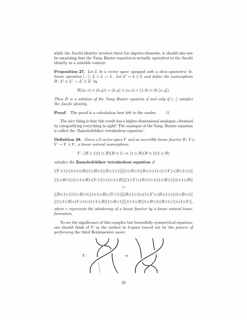
To see the significance of this complex but beautifully symmetrical equation,one should think of Y as the surface in 4-space traced out by the process ofperforming the third Reidemeister move:

Y :

%%%%%%⇒

23

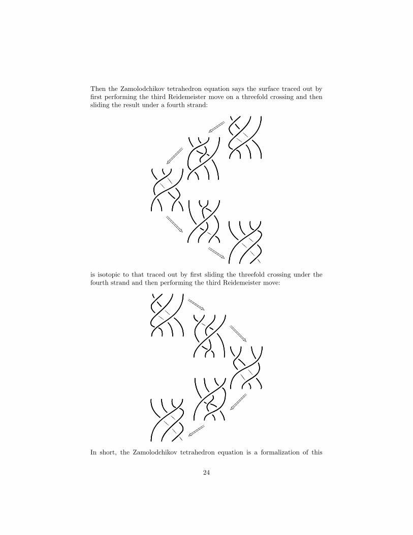
Then the Zamolodchikov tetrahedron equation says the surface traced out byfirst performing the third Reidemeister move on a threefold crossing and thensliding the result under a fourth strand:

HHBB

777;;

LLCC

BB

77;;

v~ tttttttttttt

{� �������

�������

�#???????

???????

(JJJJJJ

JJJJJJ

is isotopic to that traced out by first sliding the threefold crossing under thefourth strand and then performing the third Reidemeister move:

HHBB

LL

777;;

CCBB

77;;

(JJJJJJ

JJJJJJ

�#???????

???????

{� �������

�������

v~ tttttttttttt

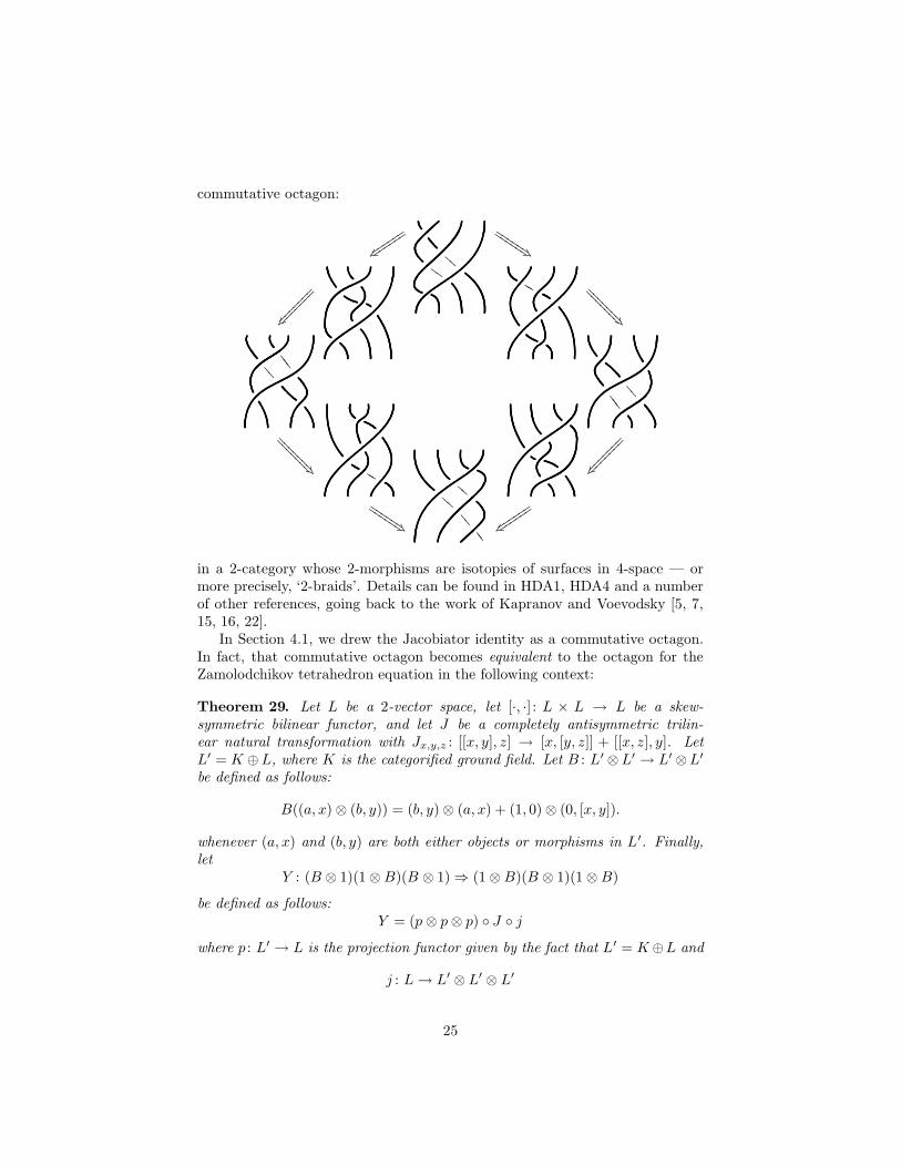
In short, the Zamolodchikov tetrahedron equation is a formalization of this

24

commutative octagon:

HHBB

777;;

LL

LL

777;;

CCBB

77;;

v~ tttttttttttt

(JJJJJJ

JJJJJJ

�#???????

???????

{� �������

�������

�#???????

???????

{� �������

�������

(JJJJJJ

JJJJJJ

v~ tttttttttttt

in a 2-category whose 2-morphisms are isotopies of surfaces in 4-space — ormore precisely, ‘2-braids’. Details can be found in HDA1, HDA4 and a numberof other references, going back to the work of Kapranov and Voevodsky [5, 7,15, 16, 22].

In Section 4.1, we drew the Jacobiator identity as a commutative octagon.In fact, that commutative octagon becomes equivalent to the octagon for theZamolodchikov tetrahedron equation in the following context:

Theorem 29. Let L be a 2-vector space, let [·, ·] : L × L → L be a skew-symmetric bilinear functor, and let J be a completely antisymmetric trilin-ear natural transformation with Jx,y,z : [[x, y], z] → [x, [y, z]] + [[x, z], y]. LetL′ = K ⊕L, where K is the categorified ground field. Let B : L′ ⊗L′ → L′ ⊗L′be defined as follows:

B((a, x)⊗ (b, y)) = (b, y)⊗ (a, x) + (1, 0)⊗ (0, [x, y]).

whenever (a, x) and (b, y) are both either objects or morphisms in L′. Finally,let

Y : (B ⊗ 1)(1⊗B)(B ⊗ 1)⇒ (1⊗B)(B ⊗ 1)(1⊗B)

be defined as follows:Y = (p⊗ p⊗ p) ◦ J ◦ j

where p : L′ → L is the projection functor given by the fact that L′ = K⊕L and

j : L→ L′ ⊗ L′ ⊗ L′

25

is the linear functor defined by

j(x) = (1, 0)⊗ (1, 0)⊗ (0, x),

where x is either an object or morphism of L. Then Y is a solution of theZamolodchikov tetrahedron equation if and only if J satisfies the Jacobiatoridentity.

Proof. Equivalently, we must show that Y satisfies the Zamolodchikov tetra-hedron equation if and only if J satisfies the Jacobiator identity. Applyingthe left-hand side of the Zamolodchikov tetrahedron equation to an object(a, w) ⊗ (b, x) ⊗ (c, y) ⊗ (d, z) of L′ ⊗ L′ ⊗ L′ ⊗ L′ yields an expression con-sisting of various uninteresting terms together with one involving

J[w,x],y,z([Jw,x,z, y] + 1)(Jw,[x,z],y + J[w,z],x,y + Jw,x,[y,z]),

while applying the right-hand side produces an expression with the same unin-teresting terms, but also one involving

[Jw,x,y, z](J[w,y],x,z + Jw,[x,y],z)([Jw,y,z, x] + 1)([w, Jx,y,z] + 1)

in precisely the same way. Thus, the two sides are equal if and only if theJacobiator identity holds. The detailed calculation is quite lengthy. ut

Corollary 30. If L is a Lie 2-algebra, then Y defined as in Theorem 29 is asolution of the Zamolodchikov tetrahedron equation.

We continue by exhibiting the correlation between our semistrict Lie 2-algebras and special versions of Stasheff’s L∞-algebras.

4.3 L∞-algebras

An L∞-algebra is a chain complex equipped with a bilinear skew-symmetricbracket operation that satisfies the Jacobi identity ‘up to coherent homotopy’.In other words, this identity holds up to a specified chain homotopy, whichin turn satisfies its own identity up to a specified chain homotopy, and so onad infinitum. Such structures are also called are ‘strongly homotopy Lie al-gebras’ or ‘sh Lie algebras’ for short. Though their precursors existed in theliterature beforehand, they made their first notable appearance in a 1985 pa-per on deformation theory by Schlessinger and Stasheff [33]. Since then, theyhave been systematically explored and applied in a number of other contexts[23, 24, 28, 31].

Since 2-vector spaces are equivalent to 2-term chain complexes, as describedin Section 3, it should not be surprising that L∞-algebras are related to thecategorified Lie algebras we are discussing here. An elegant but rather highbrowway to approach this is to use the theory of operads [29]. An L∞-algebra isactually an algebra of a certain operad in the symmetric monoidal categoryof chain complexes, called the ‘L∞ operad’. Just as categories in Vect are

26

equivalent to 2-term chain complexes, strict ω-categories in Vect can be shownequivalent to general chain complexes, by a similar argument [12]. Using thisequivalence, we can transfer the L∞ operad from the world of chain complexesto the world of strict ω-category objects in Vect, and define a semistrict Lieω-algebra to be an algebra of the resulting operad.

In more concrete terms, a semistrict Lie ω-algebra is a strict ω-category Lhaving a vector space Lj of j-morphisms for all j ≥ 0, with all source, targetand composition maps being linear. Furthermore, it is equipped with a skew-symmetric bilinear bracket functor

[·, ·] : L× L→ L

which satisfies the Jacobi identity up to a completely antisymmetric trilinearnatural isomorphism, the ‘Jacobiator’, which in turn satisfies the Jacobiatoridentity up to a completely antisymmetric quadrilinear modification... and soon. By the equivalence mentioned above, such a thing is really just another wayof looking at an L∞-algebra.

Using this, one can show that a semistrict Lie ω-algebra with only identityj-morphisms for j > 1 is the same as a semistrict Lie 2-algebra! But luckily,we can prove a result along these lines without using or even mentioning theconcepts of ‘operad’, ‘ω-category’ and the like. Instead, for the sake of anaccessible presentation, we shall simply recall the definition of an L∞-algebraand prove that the 2-category of semistrict Lie 2-algebras is equivalent to a 2-category of ‘2-term’ L∞-algebras: that is, those having a zero-dimensional spaceof j-chains for j > 1.

Henceforth, all algebraic objects mentioned are considered over a fixed field kof characteristic other than 2. We make consistent use of the usual sign conven-tion when dealing with graded objects. That is, whenever we interchange some-thing of degree p with something of degree q, we introduce a sign of (−1)pq . Thefollowing conventions regarding graded vector spaces, permutations, unshuffles,etc., follow those of Lada and Markl [23].

For graded indeterminates x1, . . . , xn and a permutation σ ∈ Sn we definethe Koszul sign ε(σ) = ε(σ;x1, . . . , xn) by

x1 ∧ · · · ∧ xn = ε(σ;x1, . . . , xn) · xσ(1) ∧ · · · ∧ xσ(n),

which must be satisfied in the free graded-commutative algebra on x1, . . . , xn.This is nothing more than a formalization of what has already been said above.Furthermore, we define

χ(σ) = χ(σ;x1, . . . , xn) := sgn(σ) · ε(σ;x1, . . . , xn).

Thus, χ(σ) takes into account the sign of the permutation in Sn and the signobtained from iteration of the basic convention.

If n is a natural number and 1 ≤ j ≤ n − 1 we say that σ ∈ Sn is an(j, n− j)-unshuffle if

σ(1) ≤ σ(2) ≤ · · · ≤ σ(j) and σ(j + 1) ≤ σ(j + 2) ≤ · · · ≤ σ(n).

27

Readers familiar with shuffles will recognize unshuffles as their inverses. Ashuffle of two ordered sets (such as a deck of cards) is a permutation of theordered union preserving the order of each of the given subsets. An unshufflereverses this process. A simple example should clear up any confusion:

Example 31. When n = 3, the (1, 2)-unshuffles in S3 are:

id =

(1 2 31 2 3

), (132) =

(1 2 33 1 2

), and (12) =

(1 2 32 1 3

).

The following definition of an L∞-structure was formulated by Stasheff in1985, see [33]. This definition will play an important role in what will follow.

Definition 32. An L∞-algebra is a graded vector space V equipped with asystem {lk|1 ≤ k <∞} of linear maps lk : V ⊗k → V with deg(lk) = k− 2 whichare totally antisymmetric in the sense that

lk(xσ(1), . . . , xσ(k)) = χ(σ)lk(x1, . . . , xn) (1)

for all σ ∈ Sn and x1, . . . , xn ∈ V, and, moreover, the following generalized formof the Jacobi identity holds for 0 ≤ n <∞ :

∑

i+j=n+1

∑

σ

χ(σ)(−1)i(j−1)lj(li(xσ(1), . . . , xσ(i)), xσ(i+1), . . . , xσ(n)) = 0, (2)

where the summation is taken over all (i, n− i)-unshuffles with i ≥ 1.

While somewhat puzzling at first, this definition truly does combine theimportant aspects of Lie algebras and chain complexes. The map l1 makes Vinto a chain complex, since this map has degree −1 and equation (2) says itssquare is zero. Moreover, the map l2 resembles a Lie bracket, since it is skew-symmetric in the graded sense by equation (1). In what follows, we usuallydenote l1(x) as dx and l2(x, y) as [x, y]. The higher lk maps are related to theJacobiator, the Jacobiator identity, and the higher coherence laws that wouldappear upon further categorification of the Lie algebra concept.

To make this more precise, let us refer to an L∞-algebra V with Vn = 0for n ≥ k as a k-term L∞-algebra. Note that a 1-term L∞-algebra is simplyan ordinary Lie algebra, where l3 = 0 gives the Jacobi identity. However, ina 2-term L∞-algebra, we no longer have a trivial l3 map. Instead, equation(2) says that the Jacobi identity for the 0-chains x, y, z holds up to a term ofthe form dl3(x, y, z). We do, however, have l4 = 0, which provides us with thecoherence law that l3 must satisfy.

Since we will be making frequent use of these 2-term L∞-algebras, it will beadvantageous to keep track of their ingredients.

Lemma 33. A 2-term L∞-algebra, V, consists of the following data:

• two vector spaces V0 and V1 together with a linear map d : V1 → V0,

28

• a bilinear map l2 : Vi × Vj → Vi+j , where 0 ≤ i+ j ≤ 1,which we denote more suggestively as [·, ·],

• a trilinear map l3 : V0 × V0 × V0 → V1.

These maps satisfy:

(a) [x, y] = −[y, x],

(b) [x, h] = −[h, x],

(c) [h, k] = 0,

(d) l3(x, y, z) is totally antisymmetric in the arguments x, y, z,

(e) d([x, h]) = [x, dh],

(f) [dh, k] = [h, dk],

(g) d(l3(x, y, z)) = −[[x, y], z] + [[x, z], y] + [x, [y, z]],

(h) l3(dh, x, y) = −[[x, y], h] + [[x, h], y] + [x, [y, h]],

(i) [l3(w, x, y), z] + [l3(w, y, z), x] + l3([w, y], x, z) + l3([x, z], w, y) =

[l3(w, x, z), y] + [l3(x, y, z), w] + l3([w, x], y, z)+

l3([w, z], x, y) + l3([x, y], w, z) + l3([y, z], w, x),

for all w, x, y, z ∈ V0 and h, k ∈ V1.

Proof. Note that (a)− (d) hold by equation (1) of Definition 32 while (e)− (i)follow from (2). ut

We notice that (a) and (b) are the usual skew-symmetric properties satisfiedby the bracket in a Lie algebra; (c) arises simply because there are no 2-chains.Equations (e) and (f) tell us how the differential and bracket interact, while(g) says that the Jacobi identity no longer holds on the nose, but up to chainhomotopy. We will use (g) to define the Jacobiator in the Lie 2-algebra corre-sponding to a 2-term L∞-algebra. Equation (h) will give the naturality of theJacobiator. Similarly, (i) will give the Jacobiator identity.

We continue by defining homomorphisms between 2-term L∞-algebras:

Definition 34. Let V and V ′ be 2-term L∞-algebras. An L∞-homomorphismφ : V → V ′ consists of:

• a chain map φ : V → V ′ (which consists of linear maps φ0 : V0 → V ′0 andφ1 : V1 → V ′1 preserving the differential),

• a skew-symmetric bilinear map φ2 : V0 × V0 → V ′1 ,

such that the following equations hold for all x, y, z ∈ V0, h ∈ V1 :

29

• d(φ2(x, y)) = φ0[x, y]− [φ0(x), φ0(y)]

• φ2(x, dh) = φ1[x, h]− [φ0(x), φ1(h)]

• [φ2(x, y), φ0(z)] + φ2([x, y], z) + φ1(l3(x, y, z)) = l3(φ0(x), φ0(y), φ0(z)) +[φ0(x), φ2(y, z)] + [φ2(x, z), φ0(y)] + φ2(x, [y, z]) + φ2([x, z], y)

The reader should note the similarity between this definition and that of homo-morphisms between Lie 2-algebras (Definition 23). In particular, the first twoequations say that φ2 defines a chain homotopy from [φ(·), φ(·)] to φ[·, ·], wherethese are regarded as chain maps from V ⊗ V to V ′. The third equation in theabove definition is just a chain complex version of the commutative square inDefinition 23.

To make 2-term L∞-algebras and L∞-homomorphisms between them intoa category, we must describe composition and identities. We compose a pairof L∞-homomorphisms φ : V → V ′ and ψ : V ′ → V ′′ by letting the chain mapφψ : V → V ′′ be the usual composite:

Vφ // V ′

ψ // V ′′

while defining (φψ)2 as follows:

(φψ)2(x, y) = ψ2(φ0(x), φ0(y)) + ψ1(φ2(x, y)).

This is just a chain complex version of how we compose homomorphisms betweenLie 2-algebras. The identity homomorphism 1V : V → V has the identity chainmap as its underlying map, together with (1V )2 = 0.

With these definitions, we obtain:

Proposition 35. There is a category 2TermL∞ with 2-term L∞-algebras asobjects and L∞-homomorphisms as morphisms.

Proof. We leave this an exercise for the reader. ut

Next we establish the equivalence between the category of Lie 2-algebras andthat of 2-term L∞-algebras. This result is based on the equivalence between2-vector spaces and 2-term chain complexes described in Proposition 8.

Theorem 36. The categories Lie2Alg and 2TermL∞ are equivalent.

Proof. First we sketch how to construct a functor T : 2TermL∞ → Lie2Alg.Given a 2-term L∞-algebra V we construct the Lie 2-algebra L = T (V ) asfollows.

We construct the underlying 2-vector space of L as in the proof of Proposition8. Thus L has vector spaces of objects and morphisms

L0 = V0,

L1 = V0 ⊕ V1,

30

and we denote a morphism f : x → y in L1 by f = (x, ~f ) where x ∈ V0 is the

source of f and ~f ∈ V1 is its arrow part. The source, target, and identity-assigning maps in L are given by

s(f) = s(x, ~f) = x,

t(f) = t(x, ~f) = x+ d~f,

i(x) = (x, 0),

and we have t(f) − s(f) = d~f . The composite of two morphisms in L1 is

given as in the proof of Lemma 6. That is, given f = (x, ~f) : x → y, andg = (y,~g) : y → z, we have

fg := (x, ~f + ~g).

We continue by equipping L = T (V ) with the additional structure whichmakes it a Lie 2-algebra. First, we use the degree-zero chain map l2 : V ⊗V → Vto define the bracket functor [·, ·] : L×L→ L. For a pair of objects x, y ∈ L0 wedefine [x, y] = l2(x, y), where we use the ‘l2’ notation in the L∞-algebra V toavoid confusion with the bracket in L. The bracket functor is skew-symmetricand bilinear on objects since l2 is. This is not sufficient, however. It remains todefine the bracket functor on pairs of morphisms.

We begin by defining the bracket on pairs of morphisms where one morphismis an identity. We do this as follows: given a morphism f = (x, ~f) : x→ y in L1

and an object z ∈ L0, we define

[1z, f ] := (l2(z, x), l2(z, ~f)),

[f, 1z] := (l2(x, z), l2(~f, z)).

Clearly these morphisms have the desired sources; we now verify that they alsohave the desired targets. Using the fact that t(f) = s(f)+d ~f for any morphismf ∈ L1, we see that:

t[1z, f ] = s[1z, f ] + dl2(z, ~f)

= l2(z, x) + l2(z, d~f) by (e) of Lemma 33= l2(z, x) + l2(z, y − x)= l2(z, y)

as desired, using the bilinearity of l2. Similarly we have t[f, 1z] = l2(y, z).These definitions together with the desired functoriality of the bracket force

us to define the bracket of an arbitrary pair of morphisms f : x → y, g : a → bas follows:

[f, g] = [f1y, 1ag]:= [f, 1a] [1y, g]

= (l2(x, a), l2(~f, a)) (l2(y, a), l2(y,~g))

= (l2(x, a), l2(~f, a) + l2(y,~g)).

31

On the other hand, they also force us to define it as:

[f, g] = [1xf, g1b]

:= [1x, g] [f, 1b]

= (l2(x, a), l2(x,~g)) (l2(x, b), l2(~f, b))

= (l2(x, a), l2(x,~g) + l2(~f, b)).

Luckily these are compatible! We have

l2(~f, a) + l2(y,~g) = l2(x,~g) + l2(~f, b) (3)

because the left-hand side minus the right-hand side equals l2(d~f,~g)− l2(~f, d~g),which vanishes by (f) of Lemma 33.

At this point we relax and use [·, ·] to stand both for the bracket on objectsin L and the L∞-algebra V . We will not, however, relax when it comes to themorphisms in L since [·, ·] 6= l2(·, ·) even on morphisms that are arrow parts, thatis, morphisms in ker(s). By the above calculations, the bracket of morphismsf : x→ y, g : a→ b in L is given by

[f, g] = ([x, a], l2(~f, a) + l2(y,~g))

= ([x, a], l2(x,~g) + l2(~f, b)).

The bracket [·, ·] : L × L → L is clearly bilinear on objects. Either of theabove formulas shows it is also bilinear on morphisms, since the source, targetand arrow part of a morphism depend linearly on the morphism, and the bracketin V is bilinear. The bracket is also skew-symmetric: this is clear for objects,and can be seen for morphisms if we use both the above formulas.

To show that [·, ·] : L× L→ L is a functor, we must check that it preservesidentities and composition. We first show that [1x, 1y] = 1[x,y], where x, y ∈L0. For this we use the fact that identity morphisms are precisely those withvanishing arrow part. Either formula for the bracket of morphisms gives

[1x, 1y] = ([x, y], 0)= 1[x,y].

To show that the bracket preserves composition, consider the morphisms f =(x, ~f), f ′ = (y, ~f ′), g = (a,~g), and g′ = (b, ~g′) in L1, where f : x→ y, f ′ : y → z,g : a→ b, and g′ : b→ c. We must show

[ff ′, gg′] = [f, g][f ′, g′].

On the one hand, the definitions give

[ff ′, gg′] = ([x, a], l2(~f, a) + l2(~f ′, a) + l2(z,~g) + l2(z, ~g′)),

while on the other, they give

[f, g][f ′, g′] = ([x, a], l2(~f, a) + l2(y,~g) + l2(~f ′, b) + l2(z, ~g′))

32

Therefore, it suffices to show that

l2(~f ′, a) + l2(z,~g) = l2(y,~g) + l2(~f ′, b).

After a relabelling of variables, this is just equation (3).Next we define the Jacobiator for L and check its properties. We set

Jx,y,z := ([[x, y], z], l3(x, y, z)).

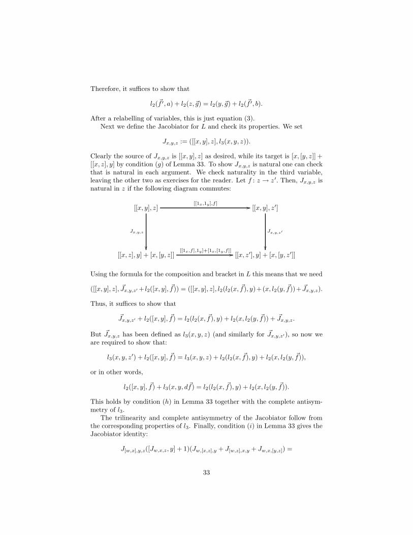
Clearly the source of Jx,y,z is [[x, y], z] as desired, while its target is [x, [y, z]] +[[x, z], y] by condition (g) of Lemma 33. To show Jx,y,z is natural one can checkthat is natural in each argument. We check naturality in the third variable,leaving the other two as exercises for the reader. Let f : z → z ′. Then, Jx,y,z isnatural in z if the following diagram commutes:

[[x, y], z][[1x,1y],f ] //

Jx,y,z

��

[[x, y], z′]

Jx,y,z′

��[[x, z], y] + [x, [y, z]]

[[1x,f ],1y]+[1x,[1y,f ]] // [[x, z′], y] + [x, [y, z′]]

Using the formula for the composition and bracket in L this means that we need

([[x, y], z], ~Jx,y,z′+ l2([x, y], ~f)) = ([[x, y], z], l2(l2(x, ~f), y)+(x, l2(y, ~f))+ ~Jx,y,z).

Thus, it suffices to show that

~Jx,y,z′ + l2([x, y], ~f) = l2(l2(x, ~f ), y) + l2(x, l2(y, ~f)) + ~Jx,y,z.

But ~Jx,y,z has been defined as l3(x, y, z) (and similarly for ~Jx,y,z′), so now weare required to show that:

l3(x, y, z′) + l2([x, y], ~f) = l3(x, y, z) + l2(l2(x, ~f), y) + l2(x, l2(y, ~f)),

or in other words,

l2([x, y], ~f) + l3(x, y, d~f) = l2(l2(x, ~f), y) + l2(x, l2(y, ~f)).

This holds by condition (h) in Lemma 33 together with the complete antisym-metry of l3.

The trilinearity and complete antisymmetry of the Jacobiator follow fromthe corresponding properties of l3. Finally, condition (i) in Lemma 33 gives theJacobiator identity:

J[w,x],y,z([Jw,x,z, y] + 1)(Jw,[x,z],y + J[w,z],x,y + Jw,x,[y,z]) =

33

[Jw,x,y, z](J[w,y],x,z + Jw,[x,y],z)([Jw,y,z, x] + 1)([w, Jx,y,z] + 1).

This completes the construction of a Lie 2-algebra T (V ) from any 2-termL∞-algebra V . Next we construct a Lie 2-algebra homomorphism T (φ) : T (V ) →T (V ′) from any L∞-homomorphism φ : V → V ′ between 2-term L∞-algebras.

Let T (V ) = L and T (V ′) = L′. We define the underlying linear functor ofT (φ) = F as in Proposition 8. To make F into a Lie 2-algebra homomorphismwe must equip it with a skew-symmetric bilinear natural transformation F2

satisfying the conditions in Definition 23. We do this using the skew-symmetricbilinear map φ2 : V0 × V0 → V ′1 . In terms of its source and arrow parts, we let

F2(x, y) = ([φ0(x), φ0(y)], φ2(x, y)).

Computing the target of F2(x, y) we have:

tF2(x, y) = sF2(x, y) + d ~F2(x, y)

= [φ0(x), φ0(y)] + dφ2(x, y)

= [φ0(x), φ0(y)] + φ0[x, y]− [φ0(x), φ0(y)]

= φ0[x, y]

= F0[x, y]

by the first equation in Definition 34 and the fact that F0 = φ0. Thus wehave F2(x, y) : [F0(x), F0(y)] → F0[x, y]. Notice that F2(x, y) is bilinear andskew-symmetric since φ2 and the bracket are. F2 is a natural transformation byTheorem 12 and the fact that φ2 is a chain homotopy from [φ(·), φ(·)] to φ([·, ·]),thought of as chain maps from V ⊗ V to V ′. Finally, the equation in Definition34 gives the commutative diagram in Definition 23, since the composition ofmorphisms corresponds to addition of their arrow parts.

We leave it to the reader to check that T is indeed a functor. Next, wedescribe how to construct a functor S : Lie2Alg→ 2TermL∞.

Given a Lie 2-algebra L we construct the 2-term L∞-algebra V = S(L) asfollows. We define:

V0 = L0

V1 = ker(s) ⊆ L1.

In addition, we define the maps lk as follows:

• l1h = t(h) for h ∈ V1 ⊆ L1.

• l2(x, y) = [x, y] for x, y ∈ V0 = L0.

• l2(x, h) = −l2(h, x) = [1x, h] for x ∈ V0 = L0 and h ∈ V1 ⊆ L1.

• l2(h, k) = 0 for h, k ∈ V1 ⊆ L1.

• l3(x, y, z) = ~Jx,y,z for x, y, z ∈ V0 = L0.

34

As usual, we abbreviate l1 as d and l2 on zero chains as [·, ·].With these definitions, conditions (a) and (b) of Lemma 33 follow from the

antisymmetry of the bracket functor. Condition (c) is automatic. Condition (d)follows from the complete antisymmetry of the Jacobiator.

For h ∈ V1 and x ∈ V0, the functoriality of [·, ·] gives

d(l2(x, h)) = t([1x, h])= [t(1x), t(h)]= [x, dh],

which is (e) of Lemma 33. To obtain (f), 33, we let h : 0→ x and k : 0→ y beelements of V1. We then consider the following square in L× L,

0h // x

0

k

��

(0, 0)(h,10) //

(10,k)

��

(x, 0)

(1x,k)

��y (0, y)

(h,1y) // (x, y)

which commutes by definition of a product category. Since [·, ·] is a functor, itpreserves such commutative squares, so that

[0, 0][h,10] //

[10,k]

��

[x, 0]

[1x,k]

��[0, y]

[h,1y] // [x, y]

commutes. Since [h, 10] and [10, k] are easily seen to be identity morphisms, thisimplies [h, 1y] = [1x, k]. This means that in V we have l2(h, y) = l2(x, k), or,since y is the target of k and x is the target of h, simply l2(h, dk) = l2(dh, k),which is (f) of Lemma 33.

Since Jx,y,z : [[x, y], z]→ [x, [y, z]] + [[x, z], y], we have

d(l3(x, y, z)) = t( ~Jx,y,z)= (t− s)(Jx,y,z)= [x, [y, z]] + [[x, z], y]− [[x, y], z],

which gives (g) of Lemma 33. The naturality of Jx,y,z implies that for anyf : z → z′, we must have

[[1x, 1y], f ] Jx,y,z′ = Jx,y,z ([[1x, f ], 1y] + [1x, [1y, f ]]).

35

This implies that in V we have

l2([x, y], ~f) + l3(x, y, z′ − z) = l2(l2(x, ~f ), y) + l2(x, l2(y, ~f)),

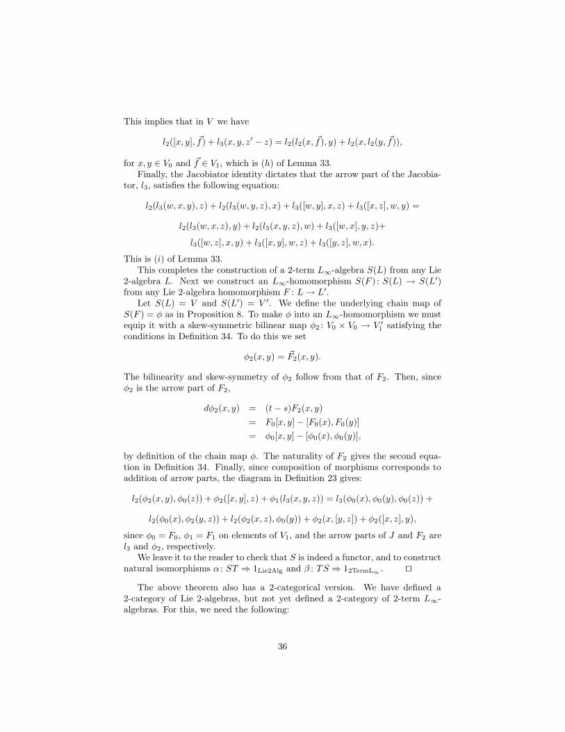
for x, y ∈ V0 and ~f ∈ V1, which is (h) of Lemma 33.Finally, the Jacobiator identity dictates that the arrow part of the Jacobia-

tor, l3, satisfies the following equation:

l2(l3(w, x, y), z) + l2(l3(w, y, z), x) + l3([w, y], x, z) + l3([x, z], w, y) =

l2(l3(w, x, z), y) + l2(l3(x, y, z), w) + l3([w, x], y, z)+

l3([w, z], x, y) + l3([x, y], w, z) + l3([y, z], w, x).

This is (i) of Lemma 33.This completes the construction of a 2-term L∞-algebra S(L) from any Lie

2-algebra L. Next we construct an L∞-homomorphism S(F ) : S(L) → S(L′)from any Lie 2-algebra homomorphism F : L→ L′.

Let S(L) = V and S(L′) = V ′. We define the underlying chain map ofS(F ) = φ as in Proposition 8. To make φ into an L∞-homomorphism we mustequip it with a skew-symmetric bilinear map φ2 : V0 × V0 → V ′1 satisfying theconditions in Definition 34. To do this we set

φ2(x, y) = ~F2(x, y).

The bilinearity and skew-symmetry of φ2 follow from that of F2. Then, sinceφ2 is the arrow part of F2,

dφ2(x, y) = (t− s)F2(x, y)

= F0[x, y]− [F0(x), F0(y)]

= φ0[x, y]− [φ0(x), φ0(y)],

by definition of the chain map φ. The naturality of F2 gives the second equa-tion in Definition 34. Finally, since composition of morphisms corresponds toaddition of arrow parts, the diagram in Definition 23 gives:

l2(φ2(x, y), φ0(z)) + φ2([x, y], z) + φ1(l3(x, y, z)) = l3(φ0(x), φ0(y), φ0(z)) +

l2(φ0(x), φ2(y, z)) + l2(φ2(x, z), φ0(y)) + φ2(x, [y, z]) + φ2([x, z], y),

since φ0 = F0, φ1 = F1 on elements of V1, and the arrow parts of J and F2 arel3 and φ2, respectively.

We leave it to the reader to check that S is indeed a functor, and to constructnatural isomorphisms α : ST ⇒ 1Lie2Alg and β : TS ⇒ 12TermL∞ . ut

The above theorem also has a 2-categorical version. We have defined a2-category of Lie 2-algebras, but not yet defined a 2-category of 2-term L∞-algebras. For this, we need the following:

36

Definition 37. Let V and V ′ be 2-term L∞-algebras and let φ, ψ : V → V ′ beL∞-homomorphisms. An L∞-2-homomorphism τ : φ ⇒ ψ is a chain homo-topy such that the following equation holds for all x, y ∈ V0:

• φ2(x, y)− ψ2(x, y) = [φ0(x), τ(y)] + [τ(x), ψ0(y)]− τ([x, y])

We leave it as an exercise for the reader to define vertical and horizontal com-position for these 2-homomorphisms, to define identity 2-homomorphisms, andto prove the following:

Proposition 38. There is a strict 2-category 2TermL∞ with 2-term L∞-algebras as objects, homomorphisms between these as morphisms, and 2-homo-morphisms between those as 2-morphisms.

With these definitions one can strengthen Theorem 36 as follows:

Theorem 39. The 2-categories Lie2Alg and 2TermL∞ are 2-equivalent.

The main benefit of the results in this section is that they provide us withanother method to create examples of Lie 2-algebras. Instead of thinking of aLie 2-algebra as a category equipped with extra structure, we may work with a2-term chain complex endowed with the structure described in Lemma 33. Inthe next two sections we investigate the results of trivializing various aspects ofa Lie 2-algebra, or equivalently of the corresponding 2-term L∞-algebra.

5 Strict Lie 2-algebras

A ‘strict’ Lie 2-algebra is a categorified version of a Lie algebra in which all lawshold as equations, not just up to isomorphism. In a previous paper [2] one of theauthors showed how to construct these starting from ‘strict Lie 2-groups’. Herewe describe this process in a somewhat more highbrow manner, and explain howthese ‘strict’ notions are special cases of the semistrict ones described here.

Since we only weakened the Jacobi identity in our definition of ‘semistrict’Lie 2-algebra, we need only require that the Jacobiator be the identity to recoverthe ‘strict’ notion:

Definition 40. A semistrict Lie 2-algebra is strict if its Jacobiator is the iden-tity.

Similarly, requiring that the bracket be strictly preserved gives the notion of‘strict’ homomorphism between Lie 2-algebras:

Definition 41. Given semistrict Lie 2-algebras L and L′, a homomorphismF : L→ L′ is strict if F2 is the identity.

Proposition 42. Lie2Alg contains a sub-2-category SLie2Alg with strict Lie2-algebras as objects, strict homomorphisms between these as morphisms, andarbitrary 2-homomorphisms between those as 2-morphisms.

37

Proof. One need only check that if the homomorphisms F : L → L′ andG : L′ → L′′ have F2 = 1, G2 = 1, then their composite has (FG)2 = 1. ut

The following proposition shows that strict Lie 2-algebras as defined hereagree with those as defined previously [2]:

Proposition 43. The 2-category SLie2Alg is isomorphic to the 2-category LieAlgCatconsisting of categories, functors and natural transformations in LieAlg.

Proof. This is just a matter of unravelling the definitions. ut

Just as Lie groups have Lie algebras, ‘strict Lie 2-groups’ have strict Lie2-algebras. Before we can state this result precisely, we must recall the conceptof a strict Lie 2-group, which was treated in greater detail in HDA5:

Definition 44. We define SLie2Grp to be the strict 2-category LieGrpCatconsisting of categories, functors and natural transformations in LieGrp. Wecall the objects in this 2-category strict Lie 2-groups; we call the morphismsbetween these strict homomorphisms, and we call the 2-morphisms betweenthose 2-homomorphisms.

Proposition 45. There exists a unique 2-functor

d : SLie2Grp→ SLie2Alg

such that:

1. d maps any strict Lie 2-group C to the strict Lie 2-algebra dC = c forwhich c0 is the Lie algebra of the Lie group of objects C0, c1 is the Liealgebra of the Lie group of morphisms C1, and the maps s, t : c1 → c0,i : c0 → c1 and ◦ : c1 ×c0 c1 → c1 are the differentials of those for C.

2. d maps any strict Lie 2-group homomorphism F : C → C ′ to the strict Lie2-algebra homomorphism dF : c→ c′ for which (dF )0 is the differential ofF0 and (dF )1 is the differential of F1.

3. d maps any strict Lie 2-group 2-homomorphism α : F ⇒ G where F,G : C →C ′ to the strict Lie 2-algebra 2-homomorphism dα : dF ⇒ dG for whichthe map dα : c0 → c1 is the differential of α : C0 → C1.

Proof. The proof of this long-winded proposition is a quick exercise in internalcategory theory: the well-known functor from LieGrp to LieAlg preserves pull-backs, so it maps categories, functors and natural transformations in LieGrp tothose in LieAlg, defining a 2-functor d : SLie2Grp → SLie2Alg, which is givenexplicitly as above. ut

We would like to generalize this theorem and define the Lie 2-algebra notjust of a strict Lie 2-group, but of a general Lie 2-group as defined in HDA5.However, this may require a weaker concept of Lie 2-algebra than that studiedhere.

38

A nice way to obtain strict Lie 2-algebras is from ‘differential crossed mod-ules’. This construction resembles one in HDA5, where we obtained strict Lie2-groups from ‘Lie crossed modules’. We recall that construction here beforestating its Lie algebra analogue.

Starting with a strict Lie 2-group C, with Lie groups C0 of objects and C1

of morphisms, we construct a pair of Lie groups

G = C0, H = ker(s) ⊆ C1

where s : C1 → C0 is the source map. We then restrict the target map to ahomomorphism

t : H → G.

In addition to the usual action of G on itself by conjugation, we have an actionof G on H ,

α : G→ Aut(H),

defined byα(g)(h) = i(g)hi(g)−1.

where i : C0 → C1 is the identity-assigning map. The target map is equivariantwith respect to this action, meaning:

t(α(g))(h) = gt(h)g−1.

We also have the ‘Peiffer identity’:

α(t(h))(h′) = hh′h−1

for all h, h′ ∈ H . So, we obtain the Lie group version of a crossed module:

Definition 46. A Lie crossed module is a quadruple (G,H, t, α) consistingof Lie groups G and H, a homomorphism t : H → G, and an action α of G onH (that is, a homomorphism α : G→ Aut(H)) satisfying

t(α(g)(h)) = g t(h) g−1

andα(t(h))(h′) = hh′h−1

for all g ∈ G and h, h′ ∈ H.

In Proposition 32 of HDA5 we sketched how one can reconstruct a strict Lie2-group from its Lie crossed module.

For a Lie algebra analogue of this result, we should replace the Lie groupAut(H) by the Lie algebra der(h) consisting of all ‘derivations’ of h, that is, alllinear maps f : h→ h such that

f([y, y′]) = [f(y), y′] + [y, f(y′)].

39

Definition 47. An infinitesimal crossed module is a quadruple (g, h, t, α)consisting of Lie algebras g and h, a homomorphism t : h→ g, and an action αof g as derivations of h (that is, a homomorphism α : g→ der(h)) satisfying

t(α(x)(y)) = [x, t(y)]

andα(t(y))(y′) = [y, y′]

for all x ∈ g and y, y′ ∈ h.

Infinitesimal crossed modules first appeared in the work of Gerstenhaber[20] where he classified them using the 3rd Lie algebra cohomology group of g.We shall see a similar classification of Lie 2-algebras in Corollary 56. Indeed,differential crossed modules are essentially the same as strict Lie 2-algebras:

Proposition 48. Given a strict Lie 2-algebra c, there is a infinitesimal crossedmodule (g, h, t, α) where g = c0, h = ker(s), t : h → g is the restriction of thetarget map from c1 to h, and

α(x)(y) = [1x, y].

Conversely, we can reconstruct any strict Lie 2-algebra up to isomorphism fromits differential crossed module.

Proof. The proof is analogous to the standard one relating 2-groups andcrossed modules [6, 19]. ut

The diligent reader can improve this proposition by defining morphisms and 2-morphisms for infinitesimal crossed modules, and showing this gives a 2-categoryequivalent to the 2-category SLie2Alg.

Numerous examples of Lie crossed modules are described in Section 8.4 ofHDA5. Differentiating them gives examples of infinitesimal crossed modules,and hence strict Lie 2-algebras.

6 Skeletal Lie 2-algebras

A semistrict Lie 2-algebra is strict when we assume the map l3 vanishes in thecorresponding L∞-algebra, since this forces the Jacobiator to be the identity.We now investigate the consequences of assuming the differential d vanishes inthe corresponding L∞-algebra. Thanks to the formula

d~f = t(f)− s(f),

this implies that the source of any morphism in the Lie 2-algebra equals itstarget. In other words, the Lie 2-algebra is skeletal:

Definition 49. A category is skeletal if isomorphic objects are equal.

40

Skeletal categories are useful in category theory because every category isequivalent to a skeletal one formed by choosing one representative of each iso-morphism class of objects [26]. The same sort of thing is true in the context of2-vector spaces:

Lemma 50. Any 2-vector space is equivalent, as an object of 2Vect, to a skele-tal one.

Proof: Using the result of Theorem 12 we may treat our 2-vector spaces as2-term chain complexes. In particular, a 2-vector space is skeletal if the cor-responding 2-term chain complex has vanishing differential, and two 2-vectorspaces are equivalent if the corresponding 2-term chain complexes are chain ho-motopy equivalent. So, it suffices to show that any 2-term chain complex is chainhomotopy equivalent to one with vanishing differential. This is well-known, butthe basic idea is as follows. Given a 2-term chain complex

C1d // C0

we express the vector spaces C0 and C1 as C0 = im(d)⊕C ′0 and C1 = ker(d)⊕Xwhere X is a vector space complement to ker(d) in C1. This allows us to definea 2-term chain complex C ′ with vanishing differential:

C ′1 = ker(d)0 // C ′0 .

The inclusion of C ′ in C can easily be extended to a chain homotopy equivalence.ut

Using this fact we obtain a result that will ultimately allow us to classify Lie2-algebras:

Proposition 51. Every Lie 2-algebra is equivalent, as an object of Lie2Alg, toa skeletal one.

Proof: Given a Lie 2-algebra L we may use Lemma 50 to find an equivalencebetween the underlying 2-vector space of L and a skeletal 2-vector space L′. Wemay then use this to transport the Lie 2-algebra structure from L to L′, andobtain an equivalence of Lie 2-algebras between L and L′. ut

It is interesting to observe that a skeletal Lie 2-algebra that is also strictamounts to nothing but a Lie algebra L0 together with a representation ofL0 on a vector space L1. This is the infinitesimal analogue of how a strictskeletal 2-group G consists of a group G0 together with an action of G0 asautomorphisms of an abelian group G1. Thus, the representation theory ofgroups and Lie algebras is automatically subsumed in the theory of 2-groupsand Lie 2-algebras!

To generalize this observation to other skeletal Lie 2-algebras, we recall somebasic definitions concerning Lie algebra cohomology:

41

Definition 52. Let g be a Lie algebra and ρ a representation of g on the vectorspace V . Then a V-valued n-cochain ω on g is a totally antisymmetric map

ω : g⊗n → V.

The vector space of all n-cochains is denoted by Cn(g, V ). The coboundaryoperator δ : Cn(g, V )→ Cn+1(g, V ) is defined by:

(δω)(v1, v2, . . . , vn+1) :=

n+1∑

i=1

(−1)i+1ρ(vi)ω(v1, . . . , vi, . . . , vn+1)

+∑

1≤j<k≤n+1

(−1)j+kω([vj , vk], v1, . . . , vj , . . . , vk, . . . , vn+1),

Proposition 53. The Lie algebra coboundary operator δ satisfies δ2 = 0.

Definition 54. A V -valued n-cochain ω on g is an n-cocycle when δω = 0and an n-coboundary if there exists an (n−1)-cochain θ such that ω = δθ. Wedenote the groups of n-cocycles and n-coboundaries by Zn(g, V ) and Bn(g, V )respectively. The nth Lie algebra cohomology group Hn(g, V ) is defined by

Hn(g, V ) = Zn(g, V )/Bn(g, V ).

The following result illuminates the relationship between Lie algebra coho-mology and L∞-algebras.

Theorem 55. There is a one-to-one correspondence between L∞-algebras con-sisting of only two nonzero terms V0 and Vn, with d = 0, and quadruples(g, V, ρ, ln+2) where g is a Lie algebra, V is a vector space, ρ is a represen-tation of g on V , and ln+2 is a (n+ 2)-cocycle on g with values in V .

Proof.(⇒) Given such an L∞-algebra V we set g = V0. V0 comes equipped with abracket as part of the L∞-structure, and since d is trivial, this bracket satisfiesthe Jacobi identity on the nose, making g into a Lie algebra. We define V = Vn,and note that the bracket also gives a map ρ : g⊗ V → V , defined by ρ(x)f =[x, f ] for x ∈ g, f ∈ V . We have

ρ([x, y])f = [[x, y], f ]= [[x, f ], y] + [x, [y, f ]] by (2) of Definition 32= [ρ(x)f, y] + [x, ρ(y)f ]

for all x, y ∈ g and f ∈ V , so that ρ is a representation. Finally, the L∞structure gives a map ln+2 : g⊗(n+2) → V which is in fact a (n+ 2)-cocycle. Tosee this, note that

0 =∑

i+j=n+4

∑

σ

lj(li(xσ(1), . . . , xσ(i)), xσ(i+1), . . . , xσ(n+2))

42

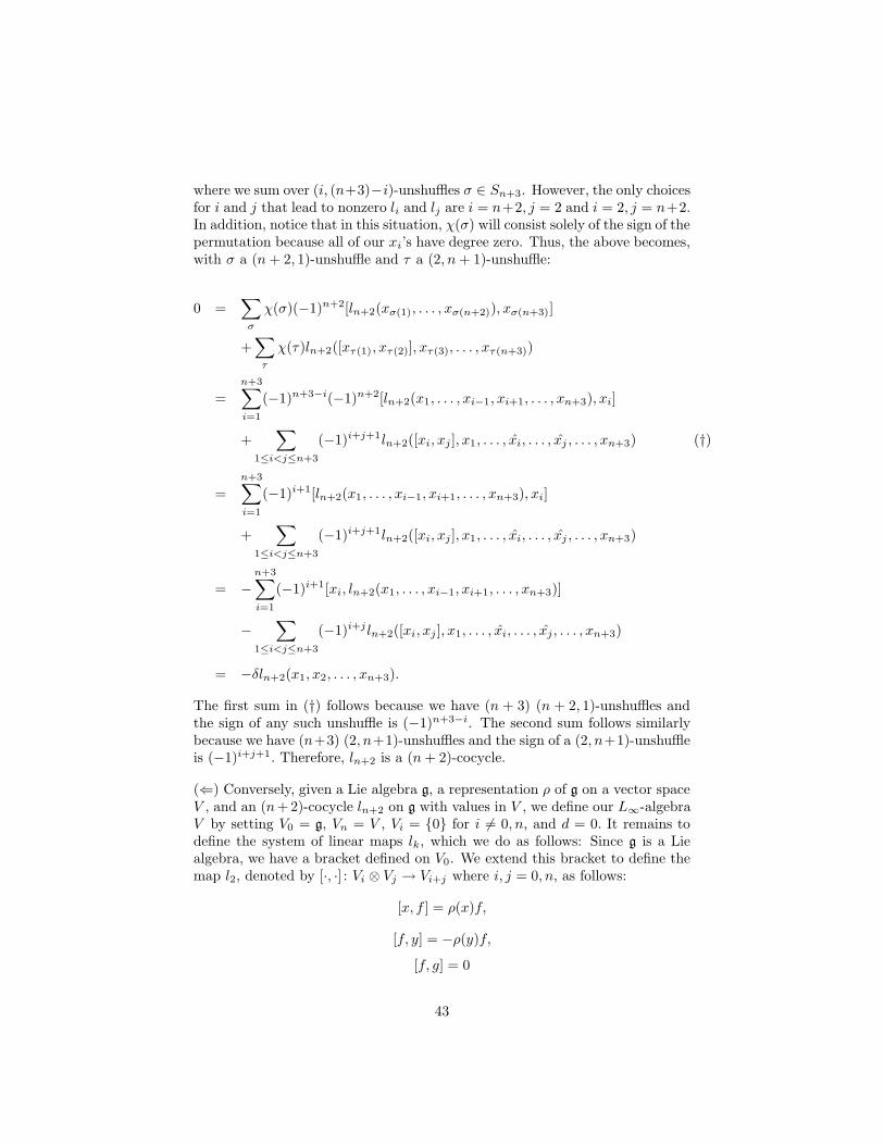
where we sum over (i, (n+3)−i)-unshuffles σ ∈ Sn+3. However, the only choicesfor i and j that lead to nonzero li and lj are i = n+2, j = 2 and i = 2, j = n+2.In addition, notice that in this situation, χ(σ) will consist solely of the sign of thepermutation because all of our xi’s have degree zero. Thus, the above becomes,with σ a (n+ 2, 1)-unshuffle and τ a (2, n+ 1)-unshuffle:

0 =∑

σ

χ(σ)(−1)n+2[ln+2(xσ(1), . . . , xσ(n+2)), xσ(n+3)]

+∑

τ

χ(τ)ln+2([xτ(1), xτ(2)], xτ(3), . . . , xτ(n+3))

=

n+3∑

i=1

(−1)n+3−i(−1)n+2[ln+2(x1, . . . , xi−1, xi+1, . . . , xn+3), xi]

+∑

1≤i<j≤n+3

(−1)i+j+1ln+2([xi, xj ], x1, . . . , xi, . . . , xj , . . . , xn+3) (†)

=

n+3∑

i=1

(−1)i+1[ln+2(x1, . . . , xi−1, xi+1, . . . , xn+3), xi]

+∑

1≤i<j≤n+3

(−1)i+j+1ln+2([xi, xj ], x1, . . . , xi, . . . , xj , . . . , xn+3)

= −n+3∑

i=1

(−1)i+1[xi, ln+2(x1, . . . , xi−1, xi+1, . . . , xn+3)]

−∑

1≤i<j≤n+3

(−1)i+j ln+2([xi, xj ], x1, . . . , xi, . . . , xj , . . . , xn+3)

= −δln+2(x1, x2, . . . , xn+3).

The first sum in (†) follows because we have (n + 3) (n + 2, 1)-unshuffles andthe sign of any such unshuffle is (−1)n+3−i. The second sum follows similarlybecause we have (n+3) (2, n+1)-unshuffles and the sign of a (2, n+1)-unshuffleis (−1)i+j+1. Therefore, ln+2 is a (n+ 2)-cocycle.

(⇐) Conversely, given a Lie algebra g, a representation ρ of g on a vector spaceV , and an (n+ 2)-cocycle ln+2 on g with values in V , we define our L∞-algebraV by setting V0 = g, Vn = V , Vi = {0} for i 6= 0, n, and d = 0. It remains todefine the system of linear maps lk, which we do as follows: Since g is a Liealgebra, we have a bracket defined on V0. We extend this bracket to define themap l2, denoted by [·, ·] : Vi ⊗ Vj → Vi+j where i, j = 0, n, as follows:

[x, f ] = ρ(x)f,

[f, y] = −ρ(y)f,

[f, g] = 0

43

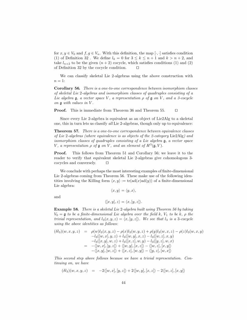
for x, y ∈ V0 and f, g ∈ Vn. With this definition, the map [·, ·] satisfies condition(1) of Definition 32 . We define lk = 0 for 3 ≤ k ≤ n + 1 and k > n + 2, andtake ln+2 to be the given (n+ 2) cocycle, which satisfies conditions (1) and (2)of Definition 32 by the cocycle condition. ut

We can classify skeletal Lie 2-algebras using the above construction withn = 1:

Corollary 56. There is a one-to-one correspondence between isomorphism classesof skeletal Lie 2-algebras and isomorphism classes of quadruples consisting of aLie algebra g, a vector space V , a representation ρ of g on V , and a 3-cocycleon g with values in V .

Proof. This is immediate from Theorem 36 and Theorem 55. ut

Since every Lie 2-algebra is equivalent as an object of Lie2Alg to a skeletalone, this in turn lets us classify all Lie 2-algebras, though only up to equivalence:

Theorem 57. There is a one-to-one correspondence between equivalence classesof Lie 2-algebras (where equivalence is as objects of the 2-category Lie2Alg) andisomorphism classes of quadruples consisting of a Lie algebra g, a vector spaceV , a representation ρ of g on V , and an element of H3(g, V ).

Proof. This follows from Theorem 51 and Corollary 56; we leave it to thereader to verify that equivalent skeletal Lie 2-algebras give cohomologous 3-cocycles and conversely. ut

We conclude with perhaps the most interesting examples of finite-dimensionalLie 2-algebras coming from Theorem 56. These make use of the following iden-tities involving the Killing form 〈x, y〉 := tr(ad(x)ad(y)) of a finite-dimensionalLie algebra:

〈x, y〉 = 〈y, x〉,and

〈[x, y], z〉 = 〈x, [y, z]〉.Example 58. There is a skeletal Lie 2-algebra built using Theorem 56 by takingV0 = g to be a finite-dimensional Lie algebra over the field k, V1 to be k, ρ thetrivial representation, and l3(x, y, z) = 〈x, [y, z]〉. We see that l3 is a 3-cocycleusing the above identities as follows:

(δl3)(w, x, y, z) = ρ(w)l3(x, y, z)− ρ(x)l3(w, y, z) + ρ(y)l3(w, x, z) − ρ(z)l3(w, x, y)−l3([w, x], y, z) + l3([w, y], x, z)− l3([w, z], x, y)−l3([x, y], w, z) + l3([x, z], w, y)− l3([y, z], w, x)

= −〈[w, x], [y, z]〉+ 〈[w, y], [x, z]〉 − 〈[w, z], [x, y]〉−〈[x, y], [w, z]〉+ 〈[x, z], [w, y]〉 − 〈[y, z], [w, x]〉

This second step above follows because we have a trivial representation. Con-tinuing on, we have

(δl3)(w, x, y, z) = −2〈[w, x], [y, z]〉+ 2〈[w, y], [x, z]〉 − 2〈[w, z], [x, y]〉

44

= −2〈w, [x, [y, z]]〉+ 2〈w, [y, [x, z]]〉 − 2〈w, [z, [x, y]]〉= −2〈w, [x, [y, z]] + [y, [z, x]] + [z, [x, y]]〉= −2〈w, 0〉= 0.

More generally, we obtain a Lie 2-algebra this way taking l3(x, y, z) = ~〈x, [y, z]〉where ~ is any element of k. We call this Lie 2-algebra g~.

It is well known that the Killing form of g is nondegenerate if and only if gis semisimple. In this case the 3-cocycle described above represents a nontrivialcohomology class when ~ 6= 0, so by Theorem 57 the Lie 2-algebra g~ is notequivalent to a skeletal one with vanishing Jacobiator. In other words, weobtain a Lie 2-algebra that is not equivalent to a skeletal strict one.

Suppose the field k has characteristic zero, the Lie algebra g is finite dimen-sional and semisimple, and V is finite dimensional. Then a version of White-head’s Lemma [1] says that H3(g, V ) = {0} whenever the representation ofg on V is nontrivial and irreducible. This places some limitations on findinginteresting examples of nonstrict Lie 2-algebras other than those of the form g~.

In HDA5 we show how the Lie 2-algebras g~ give rise to 2-groups when ~is an integer. The construction involves Chern–Simons theory. Since Chern–Simons theory is also connected to the theory of quantum groups and affine Liealgebras, it is natural to hope for a more direct link between these structuresand the Lie 2-algebras g~. After all, they are all ‘deformations’ of more familiaralgebraic structures which take advantage of the 3-cocycle 〈x, [y, z]〉 and theclosely related 2-cocycle on C∞(S1, g).

The smallest nontrivial example of the Lie 2-algebras g~ comes from g =su(2). Since su(2) is isomorphic to R3 with its usual vector cross product, andits Killing form is proportional to the dot product, this Lie 2-algebra relies solelyon familiar properties of the dot product and cross product:

x× y = −y × x,

x · y = y · x,x · (y × z) = (x× y) · z,

x× (y × z) + y × (z × x) + z × (x× y) = 0.

It will be interesting to see if this Lie 2-algebra, where the Jacobiator comesfrom the triple product, has any applications to physics. Just for fun, we workout the details again in this case:

Example 59. There is a skeletal Lie 2-algebra built using Theorem 56 by takingV0 = R3 equipped with the cross product, V1 = R, ρ the trivial representation,and l3(x, y, z) = x · (y × z). We see that l3 is a 3-cocycle as follows:

(δl3)(w, x, y, z) = −l3([w, x], y, z) + l3([w, y], x, z)− l3([w, z], x, y)−l3([x, y], w, z) + l3([x, z], w, y)− l3([y, z], w, x)

45

= −(w × x) · (y × z) + (w × y) · (x× z)− (w × z) · (x× y)−(x× y) · (w × z) + (x × z) · (w × y)− (y × z) · (w × x)

= −2(w × x) · (y × z) + 2(w × y) · (x× z)− 2(w × z) · (x× y)= −2w · (x× (y × z)) + 2w · (y × (x× z))− 2w · (z × (x× y))= −2w · (x× (y × z) + y × (z × x) + z × (x× y))= 0.

7 Conclusions

In HDA5 and the present paper we have seen evidence that the theory of Liegroups and Lie algebras can be categorified to give interesting theories of Lie2-groups and Lie 2-algebras. We expect this pattern to continue as shown inthe following tables.

n = 0 n = 1 n = 2

k = 0 manifolds Lie groupoids Lie 2-groupoids

k = 1 Lie groups Lie 2-groups Lie 3-groups

k = 2 abelian braided braidedLie groups Lie 2-groups Lie 3-groups

k = 3 ‘’ symmetric syllepticLie 2-groups Lie 3-groups

k = 4 ‘’ ‘’ symmetricLie 3-groups

k = 5 ‘’ ‘’ ‘’

1. k-tuply groupal Lie n-groupoids: expected results

n = 0 n = 1 n = 2

k = 0 vector bundles Lie algebroids Lie 2-algebroids

k = 1 Lie algebras Lie 2-algebras Lie 3-algebras

k = 2 abelian braided braidedLie algebras Lie 2-algebras Lie 3-algebras

k = 3 ‘’ symmetric syllepticLie 2-algebras Lie 3-algebras

k = 4 ‘’ ‘’ symmetricLie 3-algebras

k = 5 ‘’ ‘’ ‘’

2. k-tuply stabilized Lie n-algebroids: expected results

Table 1 gives names for k-tuply groupal n-groupoids [4] for which the set ofj-morphisms is a smooth manifold for each j, and for which the operations areall smooth. Manifolds, Lie groups and abelian Lie groups are well-understood;Lie groupoids have also been intensively investigated [27], but the study of Lie

46

2-groups has just barely begun, and the other entries in the chart are still terraincognita: they seem not to have even been defined yet, although this should beeasy for the entries in the second column.

Table 2 gives names for the ‘infinitesimal versions’ of the entries in the firstchart. The classic example is that of a Lie algebra, which can be formed bytaking the tangent space of a Lie group at the identity element. Similarly, wehave seen that the tangent 2-vector space at the identity object of a strict Lie2-group becomes a strict Lie 2-algebra; we also expect a version of this result tohold for the more general Lie 2-groups defined in HDA5, though our ‘semistrictLie 2-algebras’ may not be sufficiently general for this task.

The k = 0 row of Table 2 is a bit different from the rest. For example, amanifold does not have a distinguished identity element at which to take thetangent space. To deal with this we could work instead with pointed manifolds,but another option is to take the tangent space at every point of a manifold andform the tangent bundle, which is a vector bundle. Similarly, a Lie groupoiddoes not have a distinguished ‘identity object’, so the concept of ‘Lie algebroid’[27] must be defined a bit subtly. The same will be true of Lie n-groupoids andtheir Lie n-algebroids. For this reason it may be useful to treat the k = 0 rowseparately and use the term ‘k-tuply stabilized Lie n-algebra’ for what we arecalling a (k + 1)-tuply stabilized Lie n-algebroid.

The general notion of ‘k-tuply stabilized Lie n-algebra’ has not yet beendefined, but at least we understand the ‘semistrict’ ones: as explained in Section4.3, these are just various sorts of L∞-algebra with their underlying n-term chaincomplexes reinterpreted as strict (n− 1)-categories in Vect. More precisely, wedefine a semistrict k-tuply stabilized Lie n-algebra to be the result oftaking an L∞-algebra V with Vi = 0 when i < k or i ≥ n + k and transferringall the structure on its underlying n-term chain complex to the correspondingstrict (n− 1)-category in Vect.

In this language, Theorem 55 gives a way of constructing a semistrict Lien-algebra with only nontrivial objects and n-morphisms from an (n+2)-cocycleon the Lie algebra of objects. This can be seen as an infinitesimal version ofthe usual ‘Postnikov tower’ construction of a connected homotopy (n+ 1)-typewith only π1 and πn+1 nonzero from an (n + 2)-cocycle on the group π1. Theanalogy comes into crisper focus if we think of a connected homotopy (n + 1)-type as an ‘n-group’. Then the Postnikov construction gives an n-group withonly nontrivial objects and n-morphisms from an (n+ 2)-cocycle on the groupof objects; now the numbering scheme perfectly matches that for Lie n-algebras.For n = 2 we described how this works more explicitly in HDA5. One of thegoals of the present paper was to show that just as group cohomology arisesnaturally in the classification of n-groups, Lie algebra cohomology arises in theclassification of Lie n-algebras.

Acknowledgements

We thank Ronnie Brown, James Dolan, Vyjayanthi Chari, Andree Ehresmann,Aaron Lauda, Thomas Larsson and James Stasheff for helpful discussions and

47

correspondence. We also thank J. Scott Carter and Masahico Saito for lettingus use pictures of the Zamolodchikov tetrahedron equation taken from theirbook [15], and even adapting these pictures specially for us. Finally, we thankBehrang Noohi [30] and Dmitry Roytenberg [32] for helping us catch and fixsome significant errors in this paper.

References

[1] J. A. de Azcarraga, J.M. Izquierdo, and J. C. Perez Bueno, An introductionto some novel applications of Lie algebra cohomology in mathematics andphysics, available as physics/9803046.

[2] J. Baez, Higher Yang-Mills Theory, available as hep-th/9808101.

[3] J. Baez, Higher-dimensional algebra II: 2-Hilbert spaces, Adv. Math. 127(1997), 125–189. Also available as q-alg/9609018.

[4] J. Baez and J. Dolan, Categorification, in Higher Category Theory, eds.E. Getzler and M. Kapranov, Contemporary Mathematics vol. 230, AMS,Providence. Also available as math/9802029.

[5] J. Baez and L. Langford, Higher-dimensional algebra IV: 2-tangles, Adv.Math. 180 (2003), 705–764. Also available as math/9811139.

[6] J. Baez and A. Lauda, Higher-dimensional algebra V: 2-groups, Th. Appl.Cat. 12 (2004), 423–491. Also available as math/0307200.

[7] J. Baez and M. Neuchl, Higher-dimensional algebra I: braided monoidal cat-egories, Adv. Math. 121 (1996), 196–244. Also available as q-alg/9511013.

[8] J. Barrett and M. Mackaay, personal communication.

[9] J. Birman, Braids, Links, and Mapping Class Groups, Princeton U. Press,Princeton, 1974.

[10] F. Borceux, Handbook of Categorical Algebra 1: Basic Category Theory,Cambridge U. Press, Cambridge, 1994.

[Bre] L. Breen, Theorie de Schreier superieure, Ann. Sci. Ecole Norm. Sup. 25(1992), 465–514.

[11] R. Brown, Groupoids and crossed objects in algebraic topology, Ho-mology, Homotopy and Applications 1 (1999), 1–78. Available athttp://www.math.rutgers.edu/hha/volumes/1999/volume1-1.htm

[12] R. Brown and P. Higgins, Cubical abelian groups with connections areequivalent to chain complexes, Homology, Homotopy and Applications, 5(2003), 49–52.

48

[13] R. Brown and C. B. Spencer, G-groupoids, crossed modules, and the clas-sifying space of a topological group, Proc. Kon. Akad. v. Wet. 79 (1976),296–302.

[14] G. Burde and H. Zieschang, Knots, Walter de Gruyter, New York, 1985.

[15] J. S. Carter and M. Saito, Knotted Surfaces and Their Diagrams, AmericanMathematical Society, Providence, 1998.

[16] S. Crans, Generalized centers of braided and sylleptic monoidal 2-categories, Adv. Math. 136 (1998), 183-223.

[17] B. Day and R. Street, Monoidal bicategories and Hopf algebroids, Adv.Math. 129 (1997), 99–157.

[18] C. Ehresmann, Categories structurees, Ann. Ec. Normale Sup. 80 (1963).

C. Ehresmann, Categories structurees III: Quintettes et applicationscovariantes, Cahiers Top. et GD V (1963).

C. Ehresmann, Introduction to the theory of structured categories,Technical Report Univ. of Kansas at Lawrence (1966).

[19] M. Forrester-Barker, Group objects and internal categories, available asmath/0212065.

[20] M. Gerstenhaber, A uniform cohomology theory for algebras, Proc. Nat.Acad. Sci. 51 (1964), 626–629.

[21] A. Grothendieck, Categories Cofibrees Additives et Complexe CotangentRelatif, Lecture Notes in Math. 79, Springer-Verlag, New York, 1968.

[22] M. Kapranov and V. Voevodsky, 2-Categories and Zamolodchikov tetrahe-dra equations, in Proc. Symp. Pure Math. 56 Part 2 (1994), AMS, Provi-dence, pp. 177–260.

[23] T. Lada and M. Markl, Strongly homotopy Lie algebras, Comm. Alg. 23(6)(1995), 2147–2161. Also available as hep-th/9406095.

[24] T. Lada and J. Stasheff, Introduction to sh Lie algebras for physicists,Int. Jour. Theor. Phys. 32 (7) (1993), 1087–1103. Also available as hep-th/9209099.

[25] R. Lawrence, Triangulation, categories and extended field theories, inQuantum Topology, eds. R. Baadhio and L. Kauffman, World Scientific,Singapore, 1993, pp. 191-208.

[26] S. Mac Lane, Categories for the Working Mathematician, 2nd edition,Springer, Berlin, 1998.

[27] K. Mackenzie, Lie Groupoids and Lie Algebroids in Differential Geometry,London Math. Society Lecture Notes 124, Cambridge U. Press, Cambridge,1987.

49

[28] M. Markl, Homotopy algebras via resolutions of operads, available asmath.AT/9808101.

[29] M. Markl, S. Schnider and J. Stasheff, Operads in Algebra, Topology andPhysics, AMS, Providence, Rhode Island, 2002.

[30] B. Noohi, Integrating morphisms of Lie 2-algebras, available asarXiv:0910:1818.

[31] M. Penkava, L∞ algebras and their cohomology, available as q-alg/9512014.

[32] D. Roytenberg, On weak Lie 2-algebras, available as arXiv:0712.3461.

[33] M. Schlessinger and J. Stasheff, The Lie algebra structure of tangent coho-mology and deformation theory, Jour. Pure App. Alg. 38 (1985), 313–322.

50