high voltage line pulser for a thesis in electrical
TRANSCRIPT

HIGH VOLTAGE LINE PULSER FOR
PULSED POWER TESTING
by
HEATH KEENE, B.S.E.E.
A THESIS
IN
ELECTRICAL ENGINEERING
Submitted to the Graduate Faculty of Texas Tech University in
Partial Fulfilhnent of the Requirements for
the Degree of
MASTER OF SCIENCE
IN
ELECTRICAL ENGINEERING

*o^^ ^^3e?'^*^
Copyright 2003
Heath Keene

ACKNOWLEDGEMENTS
On a personal level, I would like to first thank my parents who with their love and
support brought me through the difficult road to graduation. On a professional level, I
would like to thank Daniel Garcia, Dino Castro, Chris Hatfield, and John Walter, Their
combined talent and knowledge in the field of pulsed power made the design of the
pulser a realized dream. On an educational level, I would like to thank Dr. Dickens and
Dr. Neuber for serving on my thesis committee.
11

11
iv
V
TABLE OF CONTENTS
ACKNOWLEDGEMENTS
LIST OF TABLES
LIST OF FIGURES
CHAPTER
I. INTRODUCTION 1
1.1 Motivation for Research 1
1.2 System Overview 2
n. BACKGROUND 5
2.1 Basic Coaxial Transmission Line Theory 5
2.2 Transient Response of Transmission Lines 10
2.3 Qualitative Description of Liquid Breakdown 20
2.4 Spark Gap Design Considerations 22
m. PULSER SYSTEM DESIGN 25
3.1 Pulser System Overview 25
3.2 Pulser Design 27
3.3 Matched Load Design 33
3.4 Trigger Generator Design 36
IV. RESULTS AND DISCUSSION 40
4.1 Overview of System Performance 40
4.2 Rise Time Characterization of Pulser System 45
4.3 Characterization of the Matched Load 45
4.4 Analysis of Reflections Present in Liquid Breakdown System 48
V. CONCLUSION 52
REFERENCES 53
111

LIST OF TABLES
1.1 Charging Schemes Required for Liquid Breakdown Experiments 3
2.1 Voltage Magnitudes for the First Four Reflected Waves 13
3.1 Pulser System Specifications 26
3.2 High Voltage Characteristics of Univolt 60 26
3.3 RG-220 Coaxial Cable Characteristics 26
4.1 Calibration Constants for Capacitive Divider Voltage Probes 41
4.2 Calibration Constants for Traveling Wave Current Probes 42
4.3 Calculated Rise Times for the Pulser System 45
IV

LIST OF FIGURES
1.1 Main Discharge Chamber and Associated histrumentation 2
1.2 Charged Line Pulser Overview 4
2.1 Cross Section of Coaxial Transmission Line 5
2.2 Equivalent Circuit of a General Transmission Line 6
2.3 Simple Transmission Line Circuit 10
2.4 Voltage Versus Length for Matched Example 11
2.5 Final Voltage Versus Length for Matched Example 12
2.6 Voltage Versus Length at 37.5 ns for the Unmatched Example 14
2.7 Voltage Versus Length at 112.5 ns for the Unmatched Example 15
2.8 Voltage Versus Length at 187.5 ns for the Unmatched Example 16
2.9 Voltage Versus Length at 262.5 ns for the Unmatched Example 16
2.10 Load Voltage Versus Time for the Unmatched Example 17
2.11 A Simple Charged Line Pulse Source 18
2.12 Pulse Generated Across the Load Resistor in Figure 2.11 18
2.13 A Charged Line Pulse Source with an Uncharged Line Load 19
2.14 Load Voltage Versus Time for Charged Line Pulse Source in Figure 2.13 20
3.1 Pulser System Schematic 25
3.2 Liquid Switching Medium Spark Gap Design 29
3.3 Diagram of Completed Oil Containment Box for Transmit Side 31
3.4 Side Section of RG-220 Feed Through for Transmit Side Containment Box 32
3.5 Picture of Completed Transmit Side Containment Box 32
3.6 Inner Conductor Brass Plate Design 34
3.7 Outer Conductor Brass Plate Design 34
3.8 Diagram of Completed Oil Containment Box for Receive Side 35
3.9 Side Section of RG-220 Feed Through for Receive Side Containment Box 35
3.10 Picture of Completed Receive Side Containment Box 36
3.11 Circuit Diagram for Coaxial Capacitive Voltage Divider 37
3.12 Side Section of Capacitive Divider Housing 38

4.1 System Diagram Used in System Characterization 40
4.2 Typical System Response fi-om All Sensors for Negative Polarity Pulse 43
4.3 Typical System Response from All Sensors for Positive Polarity Pulse 44
4.4 Receive Side Voltage with Shorted Load 46
4.5 Receive Side Voltage with Matched Load 47
4.6 Receive Side Current Showing Small Signal Response of Matched Load 48
4.7 First 700 ns fi-om the Spark Gap Voltage Probe 49
4.8 Next 600 ns fi-om the Spark Gap Voltage Probe 50
VI

CHAPTER I
INTRODUCTION
1.1 Motivation for Research
Applications of high voltage engineering abound in the current technological
climate. Most of the applications involve a pulsed power delivery system to a load that
completes the application objectives. Examples can be seen in the medical field (i.e.,
CAT scans, MRI, X-Rays), defense field (i.e., RADAR, LIDAR, EMP weapons), and the
scientific research field (i.e., the Z machine, particle accelerator experiments, and nuclear
fusion experiments), to name a few.
One of the keys to creating an effective pulsed power system is providing
appropriate and robust high voltage insulation. For many years both gaseous and liquid
insulation have been used in pulsed power systems. The modem trend in pulsed power is
a movement toward reducing the volume of these systems. A system with minimized
volume benefits fi-om the increased breakdown strength of liquid insulation. Thus, there
is a resurgence of interest in the physics of liquid breakdown. Most designers using
liquid insulation utilize general design equations that come from application specific
testing data. An enhanced scientific understanding of the breakdown process will lead to
more comprehensive insulation schemes, and thus added reliability in pulsed power
systems.
The limiting factor in understanding and quantifying the physical process of
liquid breakdown lies in the temporal limits of the diagnostics used to characterize the
breakdown. Typical diagnostics include current, voltage, and optical measurements of
the breakdown process. Modem diagnostic equipment allows temporal resolution
appropriate to understanding the physics of the liquid breakdown. Using modem CCD
cameras with minimum gate times of 2 ns, and modem digitizers with maximum sample
rates of 2 GS/s or higher, the time resolution necessary for the detailed analysis of liquid
breakdown development can be achieved.

1.2 System Overview
A complete system for evaluating DC and pulsed discharges in a variety of liquid
media has been constructed at the Center for Pulsed Power and Power Electronics, Texas
Tech University. This system involves many smaller tasks that are concemed with high
speed electrical and optical instrumentation, testing chamber construction, theoretical
modeling, data analysis, and power supply construction. This thesis concems the
development of an easily configurable power supply system. The main discharge
chamber utilizes a 50 Q matched coaxial geometry that feeds a point to plane discharge
area. The power supply system must provide both pulsed and DC charging. The
following figure shows the main discharge chamber and the associated instmmentation.
Laser
a
Needle Power Supply
Td=150ns
RG-220 Coaxial Cable Main Discharge
chamber
Td=150ns
RG 220 Coaxial Cable Plane Power
Supply
High Speed CCD Camera
Figure 1.1 Main Discharge Chamber and Associated Instrumentation
RG-220 coaxial cable was selected as the power supply connection cable because
of its high voltage characteristics. Other personnel at the Center for Pulsed Power and
Power Electronics created all of the systems shown in Figure 1.1, with the exception of
the power supplies for the two sides. There are four charging schemes that the two power
suppHes must be capable of handling. Testing will be executed using single-ended DC
charging, differential DC charging, unterminated pulsed charging, and terminated pulsed
charging. Taking into account the main chamber's point plane geometry, the power
supply system must provide twelve specific charging situations to satisfy all of the testing
needs for the liquid breakdown experiments. Table 1.1 lists each of the specific charging
schemes.

Table 1.1 Charging Schemes Required for Liquid Breakdown Experiments
Testing Genre
Single Ended Charging
Differential Charging
Unterminated Pulsed Charging
Terminated Pulsed Charging
Plane
+/-DC Ground +DC -DC +Pulsed
Ground -Pulsed Ground +Pulsed
50 Ohm Terminated -Pulsed 50 Ohm Terminated
Needle
Ground +/-DC -DC +DC Ground +Pulsed
Ground -Pulsed 50 Ohm Terminated +Pulsed
50 Ohm Terminated -Pulsed
To achieve each of these charging requirements the power supply system must
each have a dual polarity power supply, DC charging resistors, a high voltage pulser, and
a high voltage 50 Q load. The power supply solution constructed at the Center for Pulsed
Power and Power Electronics uses two Glassman High Voltage, Inc. switching power
supplies to provide the dual polarity power supplies. These power supplies have a
maximum charging voltage of 150kV, and can be remotely controlled via a 0 to 10 Volt
analog contiol signal. Each switching power supply is locked into one charging polarity.
The charging resistors, the pulser, and the 50 Q load were all constructed to fit into two
11 inch by 14 inch by 16 inch mild steel boxes. The boxes were filled with Univolt 60
transformer oil for high voltage insulation, and have cable feed throughs for both the RG-
220 coaxial cable and the power supply coaxial cable from the Glassman supplies. Either
box can be used for the single ended or the differential DC testing. This is achieved by
using the Glassman power supplies and two 400 MQ high voltage resistors insulated in
the Univolt 60 oil.
To create the high voltage source for pulsed testing, a charged cable pulser was
constructed. The cable pulser uses a 233 foot piece of RG-220 coaxial cable that is DC
charged via a Glassman power supply and a 400 MQ. charging resistor. The charged
cable acts as the prime energy source for the high voltage pulse. An inner conductor to

inner conductor self-breaking spark gap initiates the high voltage pulse. Figure 1.2
shows a schematic overview of the charged line pulser.
400MOhm
+/-VDC ^
RG-220
Charging Cable
Spark Gap RG-220
Supply Cable
V
01 X F fn r—
u
Figure 1.2 Charged Line Pulser Overview
The action of the spark gap breaking connects the inner conductor of the charging
cable with the inner conductor of the supply cable. This creates one wave propagating on
the charging cable fi-om the spark gap to the charging resistor, and another wave
propagating on the supply cable fi-om the spark gap to the main chamber. The wave on
the supply cable raises fi-om its initial voltage to !/2 the DC charging voltage on the
charged cable. The wave on the charging cable lowers from the DC charging voltage to
V2 of the DC charging voltage.
For the purpose of pulsed testing, one box contains the charging resistor and the
inner conductor to inner conductor spark gap. The other box contains the pulsed testing
load. This can be a 50 Q load or a grounding strap depending on the load requirements
for that particular test.

CHAPTER II
BACKGROUND
2.1 Basic Coaxial Transmission Line Theory
In most laboratory situations the coaxial transmission line is used for both signal
and power transfer. Coaxial transmission lines provide the most robust noise rejection of
any available transmission line. In addition, the coaxial geometry confines the electric
and magnetic fields associated with the signal guided inside the transmission line. This
significantly reduces the amount of power radiated from the transmission line during
operation. These noise benefits along with the availability of commercial high voltage
coaxial lines, led to the selection of RG-220 coaxial cable as the transmission cable used
in the liquid breakdown investigations. The following figure shows the cross section of a
solid inner conductor coaxial cable.
Outer Conductor
: ; ^
Dielectric
vjti^t^^^^iai^ W ±.
Figure 2.1 Cross Section of Coaxial Transmission Line
A coaxial cable like the one shown in Figure 2.1 is usually constructed with a
soUd inner conductor of copper, a solid dielectric of a plastic like polyethylene, an outer
conductor of copper braid, and a plastic coating outside of the copper braid that protects
and seals the cable. The figure above shows two radii, which are important in calculating
the electrical parameters of a coaxial cable. Radius a is the radius of the solid copper
inner conductor, and radius b is the radius of the solid dielectric.
All ti-ansmission lines, coaxial or otherwise, act as distributed circuit elements
when used in an electrical system. The distiibuted elements represent real impedances
that characterize the cable. These impedances depend on the geometry of the

ti-ansmission tine and on the length of the transmission line for static situations. For
dynamic situations, such as a pulse propagating down the transmission line, the behavior
of the transmission line varies greatly fi-om a simple lumped parameter model.
Understanding the response of the line in the dynamic situation requires modeling the
tiansmission line as a lumped circuit with each impedance scaled by a differential length.
The typical equivalent circuit for any transmission line of a differential length is
represented in Figure 2.2 [1].
Node N
\(z.t)
R^y I. A 7. I (i Az
i-
i(/.' A z, t)
C A z v(z-Az. t)
Az
Figure 2.2 Equivalent Circuit of a General Transmission Line
Note that a differential length Az scales each discrete circuit element. This model
allows for a solution to the dynamic response of the transmission line. Each lumped
element has a specific physical correlation to the electrical characteristics of a
tiansmission line. The series resistance represents losses in the conductors due to the
finite conductivity of the material used to create the conductors. The series inductance
relates to the self-inductance of the conductors. The parallel capacitance represents the
capacitance of the transmission line structure. The parallel conductance represents the
leakage current between the conductors caused by the finite resistivity of the dielectric.
Using Kirchoff s voltage law on the circuit in Figure 2.2 we can find the following
equation

v{z+Az,t)-v{z,t)
Az = R n
m i{z,t) + L
H
m
di{z,t)
dt [2.1]
Use of Kirchoff s current law at node N gives a second equation
Az m v{z + Az,t)-C F_
m
dv{z + h.z,t) i{z + Az,t)
dt Az = 0. [2.2]
These two coupled partial differential equations, 2.1 and 2.2, allow for the current and
voltage to be solved along the line at any point in time and length. However, the
presence of the differential length and the partial differentials make these equations
difficult to solve for even simple boundary conditions. To eliminate the differential
length the limit is taken of both equations as Az approaches infinity. This results in two
coupled partial differential equations. The equation derived from Kirchoff s voltage law
now looks like
- ^ ^ < ^ = i?.(z,0 + Z ^ ^ ^ . [2.3] dz ' dt
Via the limit, the equation derived fi-om Kirchoff s current law is transformed into
- M ^ = Gv(z,0 + C ^ ^ : ^ . [2.4] dz dt
In order to eliminate the partial differentials the equations are switched to a cosine
referenced phasor notation. To tiansform the voltage and the current into phasors the
following equations are used
v(z,0 = 9ie[F(z)e^'"'] [2.5]
/(z,0 = 5Re[/(z)e^"']. [2.6]
This substitution results in two ordinary differential equations with z as the independent
variable. For the equation derived fi-om Kirchoff s voltage law the ordinary differential
equation is
dV{z)
dz = {R + jmL)I{z).
The equation derived from Kirchoff s current law is now
^^EEl = {G + jmC)V{z). dz
[2.7]
[2.8]

These ordinary differential equations are still coupled. To decouple them the following
constant is used
y = a + JP = ^{R + jmL){G + JmC). [2.9]
Using y the two coupled first order ordinary differential equations can be decoupled into
two second order ordinary differential equations
d'V{z)
dz^
d'l(z)
dz
2 . . „ . '" "-1 — 1/
2 ^
= r^v{z), [2,10]
= r ' /(^)- [2.11]
The general solution for a second order differential equation of the form given by
Equation 2.10 is
V{z) = V:e-'''+V-e''\ [2.12]
and the general solution for Equation 2.11 is
I{z) = I^^e''' +i:e'\ [2.13]
This derivation is available in many reference texts [1], and the resulting general solution
shows the behavior of sinusoidal voltage and current waves on any transmission line.
Specifically it shows that at any length on the line, a forward traveling wave and a
reverse traveling wave determine the voltage and current at that point. The
characteristics of the oscillations are determined by the y, which in turn is calculated
fi-om the values of R, G, C and L for the specific transmission line geometry. The
amplitudes of the current and voltage waveforms are related to each other via the
characteristic impedance equation [1],
^ ^R + jmL^ y JR + jmL . H] / G+jtuC 'S^G + jzuC'
If the line is assumed to be lossless then the series resistance and parallel conductance are
neglected. This is a typical assumption unless the transmission line is very long, or the
dielectric has a poor resistivity. Under the lossless assumption the characteristic
impedance equation can be reduced to [1]

z = [2.15]
The lossless assumption also simplifies a more complicated equation for phase velocity.
The phase velocity equation quantifies the velocity of a wave along the transmission line
as[l]
1 u = [2.16]
Since the tiansmission line is assumed to be lossless the phase velocity can be equated to
the velocity of a plane wave in the dielectric material; thus the phase velocity equation
can be rewritten as [1]
1 u =•
The resistance per meter, inductance per meter, conductance per meter, and
capacitance per meter for the coaxial geometry shown in Figure 2.1 can be found using
first principles. These derivations are readily available in relevant texts [1]. The
resistance per meter of a coaxial geometry transmission line is given at a specific
fi-equency as
[2.17]
R = n^ 2;rV cr.
— + -a b
The inductance per meter can be calculated for all frequencies as
L = ^^\n^-.
In a
The conductance per meter for all frequencies is given as
2;rcr G = In
\a
[2.18]
[2,19]
[2.20]
The capacitance per meter for all frequencies is
^ ^ Ine^s^ fu\
[2,21]
In \.a)

2.2 Transient Response of Transmission Lines
The previous derivation of Equation 2.12 and Equation 2.13 included an
assumption that the wave traveling on the transmission line would be a single frequency
sinusoid. Through Fourier analysis these equations can be expanded to include all
continuous time functions, including transients. Specifically in this section the analysis
will concern transmission lines that transmit or create pulses. The simplest example of a
transmission line transmitting a pulse is shown in Figure 2.3.
Re
o OK V. dc
it R,
Figure 2.3 Simple Transmission Line Circuit
When the switch in Figure 2.3 is closed a voltage wave of magnitude [1]
v: = R.
-V. dc [2.22]
R. + K
is launched traveling from the switch side of the transmission line to the load. The
velocity of this wave is given by Equation 2.17. The current magnitude of the wave is [1]
' R. [2.23]
Because of this simple relationship between the current and voltage magnitude, only the
voltage wavefonns will be discussed in the rest of the dialogue on transient response.
Once the voltage wave reaches the load side of the transmission line one of two
things can happen. First, a portion of the wave could be reflected back due to an
impedance mismatch between the characteristic impedance of the transmission line and
the impedance of the load. Second, the impedances of the load and the line could be fiilly
matched. As a result no reflected wave would be present on the line. To begin an
10

investigation into the behavior of the system transient response a fully matched condition
will be assumed. For this to be true the impedances must be
K=K=R,. [2.24]
To show the progression of the wave along the transmission line, the voltage versus the
length on the transmission line is plotted for two cases. The first case, illustrated in
Figure 2.4, shows the wave once it has propagated halfway down the line.
V = V*
v = o
1 1 1 1 1
-
1 1 1 1 1 ..
1 1 1 1
1 u — 1
•
1 1 1 1
z = 0 z=^
Figure 2.4 Voltage Versus Length for Matched Example
It is important to note that the velocity of the wave is constant according to
Equation 2.17. This results in a direct correlation between the time since the wave was
launched and the position of the wave front on the line. The second case shows the
voltage versus length on the line after the wave has reached the load. This is
demonstrated in Figure 2.5.
11

v = v;
v = o
z=0 z=i
Figure 2.5 Final Voltage Versus Length for Matched Example
Since the load was fully matched to the characteristic impedance of the
transmission line, no reflections are present after the wave reaches the load. If there had
been a mismatch then a percentage of the wave would have been reflected back into the
transmission line. This percentage of voltage reflection is determined by the voltage
reflection coefficient [1],
term [2.25] ^term + K
The result in Equation 2.25 can be between -1 and +1. For a complete short the
reflection coefficient is - 1 , and for a complete open the reflection coefficient is +1. If the
terminating impedance is larger than the characteristic impedance then the reflected wave
adds to the incoming wave's voltage magnitude. A terminating impedance that is smaller
subtracts from the incoming wave's voltage magnitude. Equation 2.25 holds no matter
which direction the wave is traveling on the transmission line. The terminating
impedance on either side is represented in the equation by i?, ^ . The reflected wave is
represented in the general solution in Equation 2.12 by the second term. This wave
travels backward from the load to the switch with a voltage magnitude of [1]
V;=Y,V:. [2.26]
r^ is determined by the mismatch between the characteristic impedance of the
transmission line and the load impedance. If the charging resistor R^ is also mismatched
to the transmission line, then the reflected wave from tiie load will create another 12

reflection. This reflection tiavels from the switch side to the load side with a voltage
magnitude of [1]
K=r,v; = r,r,v;. [2.27] This process will theoretically repeat indefinitely. In practice the reflections repeat until
resolution of the wave front is impossible.
To illustrate this process, it is insightfiil to create an example that has both a
positive and a negative voltage reflection coefficient. The voltage on the line versus
length can then be plotted for several points in time to show the temporal development of
the reflections. For this example the characteristic impedance will be
R,=50n. [2.28]
The load impedance will be smaller than the characteristic impedance and is given by
R, = - i ?„=25Q.
This load impedance results in a voltage reflection coefficient of
[2.29]
[2.30]
The charging impedance is larger than the characteristic impedance and is given by
R^=2R„=100Q. [2.31]
This results in a voltage reflection coefficient for the charging impedance of
R. 3 [2.32]
Given a charging voltage of
V,^=\QOkV, [2.33]
the voltage magnitude of each reflected wave can be calculated. The first four voltage
magnitudes are given in Table 2.1.
Table 2.1 Voltage Magnitudes for the First Four Reflected Waves
Magnitude of Initial Wave:
Magnitude of First Reflection:
Magnitude of Second Reflection:
Magnitude of Third Reflection:
Fi^=33.333A:F
v; =-\\.\nkv
F/=-3.704A:F
F;=1.235A:F
13

To complete the example, the velocity of the waves on the tiansmission line must
be calculated. Equation 2.17 shows that for a non-ferromagnetic material the velocity of
propagation depends only on the relative dielectiic constant of the material between the
outer and inner conductors of the transmission line. For the example polyethylene is
selected as the dielectric medium. Polyethylene has a relative dielectric constant of 2.2
[2]. With this information the propagation velocity of the transient wave inside the
transmission line is calculated as
w = 2.023* 10* [f]. [2.34]
Using 50 feet of cable, or 15.24 meters, the time it takes a wave to propagate from one
side of the cable to the other can be calculated. This is referred to as the one-way transit
time for the transmission line. For the example the one-way transit time is given as
_ Cable Length 1524 m _ = = — = 75.35ns = 75ns. [2.35] tt one way
2.023*10' — s
Using all of the above specifications, voltage plots of the wave can be drawn versus the
length of the transmission line for the initial wave, and the three reflected waves. To
clearly illustrate what is happening each plot will be a snapshot of the wave on the line
when it reaches '/2 the length of the line. Figure 2.6 shows the initial wave traveling
down the line from the switch to the load.
V = V^'
v = o
t = - t t oneway =^'^-^^S
_l I I I I L.
x = 0 x = x = i
Figure 2.6 Voltage Versus Length at 37.5 ns for the Unmatched Example
14

This wave is initiated on the line when the switch closes at t=0 seconds. The
voltage magnitude of the wave is shown in Table 2.1, and the velocity of propagation
down the transmission line is given in Equation 2.34. Once the wave reaches the load, at
75 ns, a negative reflection is generated. This reflection is a percentage of the incoming
wave, and the negative reflection coefficient dictates that the wave will subtiact from the
initial voltage magnitude. The first reflected wave from the load is shown in Figure 2.7.
v = v;
v = o
1 1 1 1 — [
-
1 1 1
^ = ^^^o«.war = 1 1 2 . 5 « 5
1
-
1 1 1 1 1 1 1 1 1
v = v; + v;
x = 0 x = -£ 2
X =
Figure 2.7 Voltage Versus Length at 112.5 ns for the Unmatched Example
The reflected wave travels from the load toward the charging resistor. Once it
reaches the charging resistor at 150 ns another reflection is generated. This reflection is a
percentage of the incoming wave front only, and not the entire wave. The charging
resistor is larger than the characteristic impedance of the transmission line; thus the
reflection is a positive percentage of the incoming wave. However, the incoming wave
has a negative going wave front so the reflection again subtracts from the incoming
wave's voltage magnitude. The first reflection from the charging resistor is shown in
Figure 2.8.
15

v = v:+v.- + v;
v = o
•T I I r — — 1 1 1 r
^=l^tf oneway = 1 8 7 . 5 ^
v = v;+v;
x = Q 1 X - • x = i
Figure 2.8 Voltage Versus Length at 187.5 ns for the Unmatched Example
At 225 ns the wave shown in Figure 2.8 reaches the load and another reflection is
generated. This reflection is shown in Figure 2.9.
F = Fi + v; + v^
F = 0
7 t = —tt -262.5ns
^ oneway "
_l I 1 L.
F^Fi^+Fi'+F^'+F;
x = 0 x = -£ 2
X =
Figure 2.9 Voltage Versus Length at 262.5 ns for the Unmatched Example
Using the information in the previous four figures the voltage across the load
versus time can be calculated. This is an important step in understanding a real world
system since the voltage versus length is not easily measured. The voltage that would be
measured across the load is given in Figure 2.10.
16

v = v; + v;
F = 0
/ = 0 tt one way 2tt^ one way
3tt one way
4tt
V = v; + v; + v^ + v-
one way
Figure 2.10 Load Voltage Versus Time for the Unmatched Example
Note that the voltage across the load does not specifically reveal the reflections
associated with the mismatch at the charging side of the transmission line. These
reflections do affect the voltage at the load, but they are not discretely visible in the
voltage versus time plot. This points to the importance of fully analyzing the possible
reflections in any system involving the transient response of a transmission line. Without
a voltage measurement on each side of the transmission line, the full scope of the
behavior of the transmission line is unknown. Even with two voltage measurements,
careful analysis must first be made of the ideal response to understand what the measured
voltages physically represent.
The previous example implicitly assumed that the transmission line had no initial
charge. If the transmission line does contain an initial DC charge, then the transmission
line can be used as a pulse forming line. The capacitance of the line can be charged to a
DC voltage and used as a voltage source to supply an external load. The fact that the
charge is contained in a distributed capacitance creates a response that is unlike that of a
discrete charged capacitor source. For example, consider the circuit in Figure 2.11.
17

<-
o-dc'
R it • ^
R„
Figure 2.11 A Simple Charged Line Pulse Source
When the switch is closed in Figure 2.11 at t=0 seconds a wave front is generated.
The initial voltage is split between the matched load and the transmission line. The
generated wave results from the drop in voltage from F ^ to -F^^ as the switch closes.
The tiansient moves from the switch side to the open at the other end. Once the transient
reaches the open it is negatively reflected. In the ideal case the open is a complete open,
and the reflected wave results in a final voltage magnitude of zero. This circuit can be
used to create a pulsed voltage source. The generated pulse has a magnitude of — F ^ and
a pulse length equal to twice the one-way transit time of the transmission line. Figure
2.12 shows the generated pulse across the load resistor R^.
V K 2
v,=o
~i I I r
t = 0 t = 2tt. one way
Figure 2.12 Pulse Generated Across the Load Resistor in Figure 2.11
18

There are several drawbacks to using a pulsed voltage source such as the one in
Figure 2.11. The most obvious problem is that for a matched load the transmission line
must be charged to twice the desired pulse maximum. Another inherent problem is that
the load must be matched or else transient reflections occur. These reflections will cause
distortion in the pulse shape. To drive an unmatched load with this pulsed voltage source
another piece of uncharged transmission line must be used. An example of a system
utilizing both an uncharged and charged line to create a high voltage pulse source is
shown in Figure 2.13.
j^'^^-^i^y—^°—^^^ ^ d c - = - -=E^ — I — — I —
Charged Line " " Uncharged Line
'R.
Figure 2.13 A Charged Line Pulse Source with an Uncharged Line Load
When the switch closes in the system shown above a transient wave is launched in
both directions. One wave rising from zero Volts to -F^^ travels from the switch through
the uncharged line to the load resistor. This wave constitutes the rising edge of the
generated pulse. The other wave travels on the charged line, from the switch to the
charging resistor, with a transition from F ^ to -F^^. The charging resistor is assumed to
be much larger than the characteristic impedance of the charged line, and as a result the
voltage reflection coefficient is essentially - 1 . The pulse traveling along the charged line
is negatively reflected back toward the switch resulting in the falling edge of the pulse.
The falling edge moves through the charged line and the uncharged line until it reaches
the load, ending the pulse. The following figure shows the voltage versus time across the
load resistor.
19

F, = - ^
F, =0
1
1
( "
1 1 r
2tt one way f ^
1 1 1
^ ^
1 1 1
t = 0 Switch Closes
t = tt one way ^2 ^ '•'•one way (2 "^ ^''one way I,
Figure 2.14 Load Voltage Versus Time for Charged Line Pulse Source in Figure 2.13
The voltage waveform in Figure 2.14 assumes that the load resistor is perfectly
matched to the characteristic impedance of the uncharged transmission line. The
advantage to using the uncharged transmission line in the pulse source is that even if the
load is mismatched the pulse shape will still be fully formed. The reflections from the
load mismatch will cause residual pulse reflections, but these will occur after the falling
edge of the pulse. For this to be true the charged line must be longer than the uncharged
line, and the switch must not contain a mismatch. If these two conditions are met, a
mismatch at the load will only affect the magnitude of the pulse across the load, and will
cause smaller reflected pulses after the main pulse is completed.
2.3 Qualitative Description of Liquid Breakdown
The interest in the physical mechanisms of liquid breakdown for this thesis stems
from the selection of a liquid spark gap in the pulser design. Thus a qualitative
understanding of breakdown physics helps in the design of the pulser system. There is
not an agreed upon standard for the quantitative analysis of liquid breakdown. There are
some general design equations for liquid medium spark gap design, but most of these
deal with pulse charged gaps [3]. To add to the confusion these design equations are not
20

derived from physical principles, but are approximate equations found from extensive
testing of specific situations. However, the use of a liquid switching medium is an
attiactive selection for a spark gap designer. The large hold-off strength of liquid
dielectiics allows a spark gap design to be smaller in overall volume, and allows for
smaller gap spacing than a gas medium switch for the same charging voltage. The
smaller gap spacing results in a lower on state inductance, and a potentially faster rise
time for the switch [4]. Without a specific quantitative understanding of liquid
breakdown, the most effective route in designing a Uquid medium spark gap is to
understand the qualitative breakdown process in dense gas and apply this knowledge to
the spark gap design.
The DC breakdown process in a dense gas begins when a high electric field is
applied to the gas. For a liquid it is known that the dominant mechanism that initiates the
breakdown is preexisting elections in the liquid medium [4]. Thus, for this qualitative
description of breakdown in dense gas the free electron assumption will be used. The
free elections are accelerated by the electric field toward the anode. These elections will
eventually collide with molecules of the gas medium. Depending on the kinetic energy
of the election, the collision can excite the molecule to a higher energy state, free one
electron from the molecule, or elastically collide with the molecule resulting in no change
at the atomic level [4]. The election that is freed from an ionization event accelerates
toward the anode, and produces more ionizing collisions along the way. The excited
molecules will relax from the higher energy state and emit a photon [5]. The photon can
photoionize atoms around it, resulting in more freed electrons. The result of all of these
processes is an avalanche of charge carriers moving due to the electric field. An ever
growing negative space charge accumulates near the anode, and is eventually absorbed
by the anode. The space charge leaves behind a wake of slower moving positive ions in a
positive space charge [5]. The result is a positive space charge near the anode. The
space charge augments the electric field between the electrodes increasing the ionization
rate. The new avalanches add to the positive space charge and begin a filamentary
positive streamer [5]. The head of the streamer increases the local electric field even
more, resuhing in avalanches that meet the head of the positive streamer and add to its
21

length [5]. Eventually this stieamer will bridge the gap between the electrodes. At this
point the breakdown is complete and charge carriers from both electrodes see a low
impedance channel between the electiodes. Movement of the charge carriers through the
breakdown channel creates a self sustaining breakdown. The breakdown will persist
until the external circuit can no longer supply the needed charge carriers. Although the
previous qualitative discussion concemed gaseous breakdown, most of the discussed
features are found in liquid breakdown. Thus the previous discussion can be used as a
guide to the design of liquid medium spark gaps.
2.4 Spark Gap Design Considerations
The most obvious result of using a liquid discharge as a switching mechanism is
the effect that the temporal development of the stieamer will have on the rise time of the
switch. The rise time of any spark gap is directly related to the time it takes for the
breakdown process to occur. As the stieamer progresses across the electrode gap, the
impedance between the electrodes decreases. This is a result of avalanches meeting the
head of the stieamer. Once the streamer bridges the gap the impedance collapses rapidly,
causing the main component of the spark gap rise time often referred to as the inductive
rise time [3]. After this has occurred the impedance will still be changing. The bridged
chaimel starts as a small filamentary breakdown, and it expands in radius as more charge
carriers move along it. The moving charge carriers cause ionizing collisions that add to
the size of the ionized channel. This process looks like a changing resistance over time
as the channel expands outward and increases the amount of charge carriers that can
move through the channel. The effect of the changing resistance on the rise time is often
referred to as the resistive phase of the rise time [3]. Perhaps the most important effect of
streamer breakdown on rise time is the random variation caused by the breakdown
process. The length of time between the development of the positive space charge near
the anode and the completed breakdown varies. This results in a small variance in the
rise time of the spark gap that cannot be predicted.
Most spark gaps are created with two electiodes and a dielectiic housing that
confines the switching medium inside it. When a spark gap is used in a pulser system
22

such as the one shown in Figure 2.13 the impedance of the spark gap structure becomes
important. Creating the spark gap with a coaxial geometry that is impedance matched to
the coaxial lines is imperative to reduce reflections in the system. This requirement
results in a spark gap design that contains the two electrodes and a common outer
conductor. The introduction of the outer conductor means that the spark gap could create
an undesired breakdown between one electrode and the outer conductor. The design of a
coaxial spark gap requires that erroneous breakdowns must be considered as well as the
desired main breakdown. At first glance the solution seems easy, make the path from
both electiodes to the outer conductor much longer than the path between the electrodes.
This solution does not guarantee proper operation of the switch. There are two factors
that can increase the likelihood of a breakdown between an electrode and the outer
conductor, even if the path length is much longer.
The first factor to consider is the effect of electric field enhancement.
Microscopic surface roughness can increase the local electric field, causing a more
attiactive initiation point for the streamer breakdown. The presence of another dielectric
medium in the liquid, such as an air bubble, can drastically increase the local electric
field at the interface between the bubble and the Uquid [4], Once again this creates a
more attiactive site to begin the breakdown process. Both of these factors influence the
electric field present between the inner and outer conductor for a given charging voltage.
The second factor to consider is the carbonization of transformer oil after a
breakdown has occurred [4]. The ionization process can break the covalent bonds that
hold the oil molecules together. Liberated carbon molecules lower the average resistance
of the oil. This can allow more charge carriers to move in the oil for a given charging
voltage. The movement of the charge carriers can prematurely start avalanches and result
in a lowered bulk breakdown stiength for the oil.
Another often overiooked component to liquid spark gap design is the need for
mechanical rigidity. The process of the stieamer breakdown creates intense mechanical
Shockwaves in the liquid medium. The intensity of the Shockwave is related to the
energy expended in the process of the breakdown. Research into this phenomenon has
shown that as the stieamer absorbs new avalanches and extends its length, a Shockwave is
23

created in the surrounding liquid [6]. As the streamer steps across the electrode gap the
separate Shockwaves combine through superposition. The result is a single shock front
that can destioy components of the spark gap. A completed design of a liquid spark gap
should be able to withstand repetitive abuse from these Shockwaves.
24

CHAPTER III
PULSER SYSTEM DESIGN
3.1 Pulser Svstem Overview
til Section 2.2 a scheme for creating a high speed pulser via a charged line, an
inner conductor to inner conductor spark gap and an uncharged line connected to a load
was discussed. This basic principle was used to create the pulsed supply for the liquid
breakdown experiments. Figure 3.1 shows the entire pulser system.
Coaxial Main Spark Gap Oiamber
Figure 3.1 Pulser System Schematic
Inside the main chamber the needle and plane can be configured to connect to
either of the attached coaxial cables. The configurable main chamber results in choosing
one cable to be the cable that transmits the incoming pulse and one to be the cable that
receives the incoming pulse.
Construction of the pulser system involves the design of the coaxial spark gap, the
charging resistor i?^, and the 50 Q matched high voltage loadi?^ . The length of the
charged line is determined by the pulse length requirements of the pulser system. The
length of the transmit line and receive line are closely matched. The transmit line length
is set to allow for the necessary setup time for the main chamber instrumentation. A
capacitive voltage divider placed immediately before the tiansmit line is used to scale the
voltage signal leaving the pulser. The signal from this divider is fed into a digitally
programmable delay generator via a small length of coaxial cable. The pulse from the
delay generator is used to trigger the instrumentation digitizers and the optical diagnostics
at any point before, during, or after the pulse has reached the main chamber.
The 50 Q matched load is used to assure accuracy in the receive side instiiunentation.
25

Table 3.1 shows the system specifications used to create the design for the pulser system.
Pulse Length: Table 3.1 Pulser System
Pulse Magnitude into Matched Load:
Pulse Magnitude into Open:
Rise Time:
Characteristic Impedance:
Specifications >700 ns at FWHM
0 to 60 kV Adjustable
0 to 120 kV Adjustable
<20 ns
50 Q Given these specifications the entire system can be created. The high voltage
requirements mean that the system must contain robust high voltage insulation. To
accomplish this the charging resistor, the spark gap, and the load are immersed in Univolt
60 tiansformer oil. The relevant high voltage characteristics of Univolt 60 transformer
oil are shown in Table 3.2 [2].
Table 3.2 High Voltage Characteristics of Univolt 60
Dielectric Constant:
Breakdown Strength:
^ =2.2
^*...^o.„ = 9.843xl0^ [^]^o3.937x10^ [^]
As mentioned in Section 1.2 the coaxial cable of choice for tiie liquid breakdown
experiments is RG-220. This cable exhibits excellent DC hold-off characteristics, thus it
is a natural choice for the pulser system. Table 3.3 shows the applicable characteristics
of RG-220 cable [7, 2].
Table 3.3 RG-220 Coaxial Cable Characteristics
Type of Inner Conductor:
Inner Conductor Radius:
Type of Solid Dielectric:
Solid Dielectric Radius:
Dielectric Constant:
Type of Outer Conductor:
Characteristic Impedance:
Distributed Capacitance:
Propogation Velocity:
Solid Copper
0,13 inches
Polyethylene
0.455 ± 0.0075 inches
£, = 2.2
Braided Copper
50Q
30,8 pF per foot
M = 2.023* 10' If]
26

Times Microwave manufactures this cable, and the Center for Pulsed Power and
Power Electionics at Texas Tech University has bought two large spools of the cable.
Unfortunately, the spools were purchased three years apart. This resulted in a notable
manufacturing tolerance drift in the polyethylene diameter that had to be considered
during the design of all components interfacing with the RG-220 cable. The most notable
characteristic of the RG-220 cable is that the relative dielectric constant of the
polyethylene dielectric is the same as the dielectric constant of the Univolt 60 transformer
oil. Because of this shared characteristic, the electric field across an interface of the
dielectrics will be continuous.
3.2 Pulser Design
The pulser itself is contained in the components previous to the transmit line in
Figure 3.1. In particular the pulser requires a high voltage DC power supply, the
charging resistor, the charged cable, the coaxial self-breaking spark gap, and a mild steel
box with appropriate feed throughs that contains the Univolt 60 transformer oil. As
mentioned in Section 1.2, Glassman manufactures the high voltage DC supplies used in
the design. The charging resistor selected is a single 400 MQ solid carbon high voltage
resistor manufactured by Dale. The goals in selecting this resistor are to find a resistor
that will not suffer from surface flashover during the beginning of the charging cycle, and
to find a resistance that will be much larger than 50 Q. The large resistance is needed to
provide a voltage reflection coefficient as close to 1 as possible. For a 400 MQ resistor
the voltage reflection coefficient is
^ i z i = i 5 2 ^ i ^ ^ l z ^ = 0,99999975, [3,1] • R.-t-K 400il«2 + 50n
For all practical purposes this resistor will appear as an open circuit to the impinging
pulse.
The design of the charged cable only requires a determination of the cable length,
which relates to the length of the output pulse. Using the pulse length requirement in
Table 3.1 the length of cable needed is calculated as
27

Pulse Length ^ •u = Cable Length = 232 feet. [3.2]
This calculation assumes that the pulse has an ideal rise and fall time. To assure that the
pulse length specification is met, an extra foot is added to the charged cable. For a cable
length of 233 feet the ideal pulse length is
Pulse Length = ^^^ableLength ^ ^^^^^ ^^^^
The added cable length ensures that the fiiU width half maximum (FWHM) of the pulse
will be larger than 700 ns.
The self breaking liquid medium spark gap presents the most complicated design
challenge in the pulser system. The system specifications in Table 3.1 set the rise time
requirement, the inner conductor to outer conductor hold off voltage requirement, and the
desired characteristic impedance of the spark gap. The system specifications also
necessitate an adjustable electrode gap spacing. A liquid switching medium was chosen
both for the lower rise time values associated with liquid breakdown phenomenon, and
for the high breakdown strength of liquid dielectrics. Univolt 60 was selected as the
switching medium due to its use in other parts of the design.
The starting point for the design of the spark gap is to determine how the
electrodes will be constructed. In a commercially produced spark gap electrode wear is
an important design criterion. The streamer discharge inside the spark gap ablates the
electrode material, and over time the ablations distort the original electiode shape. This
can result in local field enhancements that cause the spark gap to operate improperly. In
a liquid medium switch the ablations can be worse due to the Shockwave associated with
the breakdown. Often copper tungsten or carbon composites are used because of their
wear characteristics. The most difficult task in creating such a spark gap is not choosing
the electrode material, but creating a feed through system that interfaces the electrodes to
the driving cable. Care must be taken in creating a feed through that can withstand the
charging voltage without surface flashover. Since the spark gap for the pulser system is
to be used in a laboratory environment, electiode wear is not a major design concern.
The electrodes can be changed as needed. To eliminate the need for the high voltage feed
through, the inner conductors of the charging fine and the tiansmit line will be used as the
28

spark gap electiodes. RG-220 cable uses a solid copper inner conductor. Both electiodes
can be created by filing the edges of the inner conductor until it has a — inch curvature 16
radius.
The most complicated part of the spark gap design is creating an impedance
matched gap that can withstand a 120 kV DC charging voltage without breakdown to the
outer conductor. The first design of the switch involved a fully matched outer conductor.
The fiilly matched switch suffered from breakdown from the inner conductor to the outer
conductor at a charging voltage of « 75kV. This led to a design that sacrifices impedance
matching for the sake of hold off voltage. The outer conductor in the final design was
tapered outward to increase the bulk breakdown length. A side section of the design is
shown in Figure 3.2.
4,000 3,000 1,500 0,930
B Copper Inner
I Aluminum Outer Conductor
Polyethylene Solid Dielectric
B Univolt 60 Transformer Oil
Figure 3.2 Liquid Switchmg Medium Spark Gap Design
The outer conductor is made from two halves of machined aluminum. The halves
are held securely together via a three bolt hole pattern around the edge of the outer
conductor. The outer conductor diameter is linearly tapered, from the diameter of the
polyethylene to three inches, at a45'' angle. The outer conductor of the switch is attached
to the copper braid outer conductors of the RG-220 cables via hose clamps. The gap can 29

be adjusted by loosening one hose clamp and manually moving the cable until the desired
gap spacing is reached. The switch was designed to allow a maximum gap spacing of
one inch. The outer conductor of the switch was machined with one viewing window to
allow the user to observe the operation of the spark gap. The viewing window also
doubles as a fill hole for the Univolt 60 tiansformer oil, and it reduces the mechanical
stiain due to Shockwaves during breakdown. The polyethylene is shaped with a 45° angle
to make insertion of the cable easier. The shaping is done with a specially created tool
that slices the solid dielectric with a razor blade, while leaving the inner conductor intact.
Tapering the outer conductor of the spark gap results in an impedance mismatch.
The impedance of the gap after the outer conductor has reached the end of the taper is
given by
^b^
H-c-MoMr J ^ ^ In 2n a \aj 2ns^ 2n
F^=98.93Q, S E
or
[3,4]
In \a)
For the calculation of Equation 3.4 the inner conductor radius for RG-220 is used. This
assumes that the diameter of the streamer discharge during the switching action will not
drastically affect the impedance. In practice this assumption is incorrect and the
characteristic impedance will increase along the area of the stieamer discharge. The
radius of the stieamer changes over time and is hard to quantify; thus in most spark gap
designs Equation 3.4 is used to estimate the characteristic impedance [4].
To operate properly both the charging resistor and the spark gap must be
immersed in transformer oil. To this end a box was created to contain the transformer oil.
The box is made of mild steel and has electrical feed throughs for both RG-220 and the
power supply cable. Both types of electrical feed throughs utiUze o-rings that seal the oil
inside the box and allow the cables to pass from an air environment into the oil
environment without leaking oil from the box. The power supply cable feed throughs
employ commercially produced Cajon fittings. The RG-220 cable feed throughs were
created specifically for the experiment, and were welded into the mild steel box. After
the RG-220 feed throughs were welded in, the entire box was painted with a two-part
30
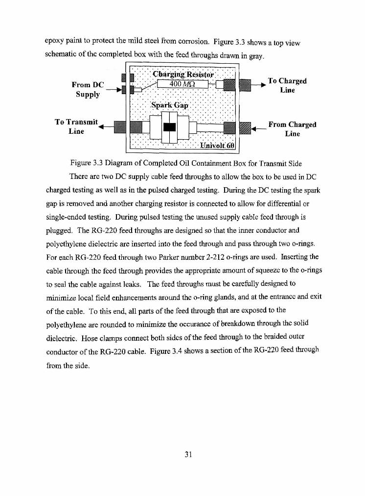
epoxy paint to protect the mild steel from corrosion. Figure 3.3 shows a top view
schematic of the completed box with the feed throughs drawn in gray.
From DC Supply
To Transmit Line
p l-r-:
, Ch^rgiuglRejsistor. •A '40bMQ - f - M
,SpkrkGap, , , , , ,
. . • , , , ujiivoittxo
To Charged Line
From Charged Line
Figure 3.3 Diagram of Completed Oil Containment Box for Transmit Side
There are two DC supply cable feed throughs to allow the box to be used in DC
charged testing as well as in the pulsed charged testing. During the DC testing the spark
gap is removed and another charging resistor is connected to allow for differential or
single-ended testing. During pulsed testing the unused supply cable feed through is
plugged. The RG-220 feed throughs are designed so that the inner conductor and
polyethylene dielectric are inserted into the feed through and pass through two o-rings.
For each RG-220 feed through two Parker number 2-212 o-rings are used. Inserting the
cable through the feed through provides the appropriate amount of squeeze to the o-rings
to seal the cable against leaks. The feed throughs must be carefully designed to
minimize local field enhancements around the o-ring glands, and at the entrance and exit
of the cable. To this end, all parts of the feed through that are exposed to the
polyethylene are rounded to minimize the occurance of breakdown through the solid
dielectric. Hose clamps connect both sides of the feed through to the braided outer
conductor of the RG-220 cable. Figure 3.4 shows a section of the RG-220 feed through
from the side.
31

Oil Side Air Side
0,187
0,4
Figure 3.4 Side Section of RG-220 Feed Through for Transmit Side Containment Box
The stepped outer diameter shown in the above figure was created to minimize
the air tiapped between the outer braided conductor and the polyethylene. If an air
pocket is present during a DC charged situation the field enhancement caused by the
pocket can create corona discharge or breakdown through the polyethylene dielectric.
The completed oil containment box with the spark gap and charging resistor installed is
shown in Figure 3.5.
Figure 3.5 Picture of Completed Transmit Side Containment Box
32

3.3 Matched Load Design
Design of the receiving side of the pulser system involves the creation of a
50Q matched load. Ideally this load would appear as a purely resistive load from the
inner conductor to the outer conductor that is fiilly matched to the characteristic
impedance of the receiving side tiansmission line, hi practice the load must be carefully
designed to minimize stiay inductance and capacitance, either of which could cause
unwanted reflections. The load must be able to handle a large signal pulse of 60 kV
without breakdown between the inner and outer conductor. Previous to the stieamer
breakdown in the main chamber small signal current prepulses are created from the
initiating avalanches of the main breakdown. Measurement of these prepulses in the
presence of reflections is difficult; thus the load must appear matched to the small signal
prepulses. The load is designed to be easily removed so that testing with a short or open
load on the received side can be achieved.
The resistance of the load is created via eight parallel chains of 2-Watt solid
carbon resistors. Previous research into the high voltage capabilities of these resistors
when insulated by tiansformer oil has shown that a single resistor can withstand 16 kV
DC before it responds nonlinearly [8]. It is assumed that this limit can be expanded
during usage in a pulsed environment. Because of this limitation, three resistors in series
generate each of the eight parallel chains. This results in a final design that uses 24
individual resistors. The resistance value for each of the individual resistors is calculated
as
50Qx#o/c/;aw5 _ 50Qx8 _ - z ^ r 5]
# in each chain 3
The closest standard resistance value is 130Q. Construction of the resistor chains starts
by measuring the individual resistance for each of the 24 resistors using the HP 4263B
LCR meter. The resistors were then individually selected so that each series chain
resistance measured 400 Q. The series chains were then soldered together. The final
resistance of the load was measured on the LCR meter as 50.1Q.
The outer conductor and inner conductor connections for the matched load were
created via two brass plates. Design of the plates centered on maximizing the breakdown
33

voltage between the plates. To this end each plate was constructed with a corona ring
around the edge of the plate. This assured that the field enhancements at the plate edges
were minimized. The parallel resistor chains are connected to each plate via set screws.
The inner conductor plate is connected to the inner conductor of the receive line via a set
screw. Screwing the outer conductor brass plate onto a threaded RG-220 feed through in
the receive side oil containment box makes the outer conductor connection. The design
for the inner conductor brass plate is shown in Figure 3.6.
1/4 inch r a d i u s
_Hole f o r r- e s i s t o r s
Threaded f o r 4-40 s e t sc rews
1hreaded f o r 4-4 0 se t s iz r e w
Threaded " fo r 4-40 se t s c r e v
- 0 0 . 2 5
Side Section Front Section Figure 3.6 Inner Conductor Brass Plate Design
The outer conductor plate design is shown in Figure 3.7.
1/4 i n c l"i r a d i u s
1/8 inch r a d i u s 01,5
-0,5
0,25
^J - ^ , Hole f o r r e s i s t o r ?
T h r e a d e d f o r 4 -40 s e t s c r e w ;
Threaded a t 20 t h r e a d s per incOi
- - ^ 3 , 5
Side Section Front Section Figure 3.7 Outer Conductor Brass Plate Design
34

The entire load assembly is immersed in transformer oil to insulate against bulk
breakdown between the electrode plates. A received side containment box was created to
hold the load and transformer oil. Construction of the box was achieved in a similar
manner to the transmit side containment box. Changes were made to the RG-220 feed
throughs to allow attachment of the outer conductor plate from the load. A top view
diagram of the receive side oil containment box is shown in Figure 3.8.
To Transmit Line for
DC Testing
From Receive Line
From DC Supply for DC Testing
Figure 3.8 Diagram of Completed Oil Containment Box for Receive Side
The receive side containment box can double as a DC testing supply. This
explains the presence of the extra RG-220 feed through and the two DC supply feed
throughs. For pulsed testing these extia feed throughs are plugged. A side section of the
RG-220 feed through with threads to connect the outer conductor of the load is shown in
Figure 3.9. Oil Side Air Side
Threaded with 20
t h r e a d s per i r c h
0.25-
Figure 3.9 Side Section of RG-220 Feed Through for Receive Side Contaimnent Box
35

The feed through shown above uses the same size o-rings as the feed throughs
used for the tiansmit side. This feed through does not contain the stepped outer diameter
because it is only exposed to a pulsed situation. This means that for DC testing the
transmit side containment box is preferable to minimize corona discharge during testing.
The second RG-220 feed through welded into the receive side containment box is
identical to the one in Figure 3.9 except for the threaded portion. A picture of the
completed oil containment box for the receive side is shown in Figure 3.10.
Figure 3.10 Picture of Completed Receive Side Containment Box
3.4 Trigger Generator Design
As discussed in Section 3.1 the trigger signal mdicating that the pulse has begun
propagation down the transmit line is created via a coaxial capacitive divider. The use of
the capacitive divider has the added benefit of allowing monitoring of the system
response from the pulser end of the transmit coaxial cable. The circuit diagram for the
capacitive voltage probe is shown in Figure 3.11.
36

V, line
A
c. ^
^ - • < ^
c.
D droop
F„
Z =50Q
measured
Rscope =50Q
Figure 3.11 Circuit Diagram for Coaxial Capacitive Voltage Divider
The incoming signal being measured is shown as ,„ in Figure 3.11. If C2 > C,
then the voltage at point Fj is attenuated by the capacitive divider. The capacitive divider
not only attenuates the signal, it also acts as a high pass filter. If R^^^^^ > OQ then the
voltage at V^ is attenuated again by the resistive divider created by R^^^^p and Z^ to
produce the measured voltage. The pulsed response of the divider circuit shown in
Figure 3.11 is of chief concern in the liquid breakdown experiments. When a pulse is
applied to the capacitive divider, only the rising edge of the pulse passes through Q to be
attenuated by the circuit. After the rising edge has passed, C, DC blocks the flat top of
the pulse. An amount of charge is left on Cj, which causes an exponential voltage decay
in the measured voltage. The decay time is set by the RC time constant calculated from
Cj and i? „„p + Z„. The exponential decay is typically referred to as the voltage droop of
the capacitive divider [4]. The falling edge of the pulse is passed byQ, again causing a
change in the amount of charge on C^ • However, the voltage droop from the rising edge
of the pulse will effect where the falling edge begins. This results in a measured pulse
that contains the correct time information, and shows the correct magnitude for the rising
and falling edge of the pulse, but incorrectiy represents the flat top response of the pulse.
37

When analyzing the output of a capacitive divider circuit it is useful to separate
the action of the attenuation from the voltage droop of the circuit. The attenuation factor
of a capacitive divider can be experimentally measured by applying a pulse of known
magnitude. The droop can also be measured via this technique, but this involves doing
complicated curve fitting on the measured signal to find the time constant. A more
straightforward approach for finding the time constant is to measure Cj and R^^^^^ using a
LCR meter, and calculate the time constant based on the measured capacitance and
resistance.
Creation of a coaxial capacitive voltage divider starts with designing an outer
conductor. The outer conductor serves as the signal ground in Figure 3.11, and houses
the capacitive divider itself The outer conductor designed for the trigger generator
capacitive divider is shown in Figure 3.12.
e N C o n n e c t o r
Figure 3.12 Side Section of Capacitive Divider Housing
The inner conductor and polyethylene dielectric are inserted into tiie housing.
The outer copper braid from the RG-220 cable is hose clamped to the outer conductor of
the divider. A rectangular piece of one inch by two inch copper shim stock is inserted
between the polyethylene and the outer housing. A piece of Mylar tape is used to
insulate the copper shim stock from the outer housing. The capacitance from the inner
conductor of the RG-220 to the copper shim creates the C, capacitance shown in Figure
3.11. The capacitance between the copper shim and the outer conductor constitutes the
38

Cj capacitance, A small connector is soldered to the copper shim and connected to one
end of the resistor that is used as R^^^^^. The other end of the resistor is connected to the
inner conductor of the Type N connector shown in Figure 3.12. The resistor fits in the
void below the Type N connector. All three voltage monitors used in the liquid
breakdown experiments employ capacitive dividers built using this constmction
technique.
39

CHAPTER IV
RESULTS AND DISCUSSION
4.1 Overview of Svstem Performance
The performance of the pulser system and the matched load are best determined
via looking at the liquid breakdown system response during actual testing. This method
can be more complicated to analyze than testing the pulser system and the load
separately; however, testing the entire system at once provides insight that cannot be
found from testing the components alone. The rise time and pulse length of the output
pulse characterize the pulser system. The performance of the load is found by examining
the reflections generated by both large signals and small signals. In particular the load is
useful in allowing resolution of phenomena both before and after breakdown in the main
chamber that would be impossible to analyze in the presence of reflections. The
impedance match of all of the included systems determines the performance of the entire
liquid breakdown experiment as a whole. For this component of the analysis the
reflections created by the main chamber, the pulser spark gap, the pulser charging
resistor, and the load are investigated via the response from each of the three sensor
positions. The time delay between each of these components must be known for a
complete investigation. The following diagram shows the necessary information for the
entire system analysis.
•H'„„.».«-153«5 >\4 = 4,5«5
1 - Spark Gap Voltage Probe 2 - Transmit Side Current and Voltage Probes 3 - Receive Side Current and Voltage Probes
Figure 4.1 System Diagram Used in System Characterization
The reflection coefficient associated with the charging resistor was already
calculated in Equation 3.1. The spark gap reflection coefficient changes depending on
40

whetiier or not the gap is bridged by a streamer discharge. Without the discharge both
sides of the spark gap looks like an open. With the switch gap bridged the reflection
coefficient is estimated by
^ 98.93Q-50Q ^SG = ^ „ ^ . , ^ . „ „ = 0 .329. 98.93Q + 50Q ^'"^^' ^^-^^
The main chamber reflection coefficient also depends on the status of the discharge
inside the chamber. Like the spark gap, the main chamber appears as an open at both
ends when the streamer discharge is not present. The main chamber was designed to be
ftilly matched when the discharge is present, but the small radius of the discharge will
present a minute impedance mismatch. A discussion of the reflections from the matched
load is presented in Section 4.3.
To obtain an accurate analysis of the measured waveforms each probe in the
system must be properly calibrated. For the three capacitive divider voltage probes the
calibration includes the determination of both the attenuation constant and the voltage
droop time constant. The attenuation constants are experimentally found by applying a
60kV pulse to the entire system shown in Figure 4.1. Using the known maximum of the
appUed pulse the attenuation constant for each probe can be calculated. The time
constant for each of the voltage probes is determined via the measurement method
discussed in Section 3.4. Table 4.1 shows the calibrations for each of the voltage probes
used in the experiment.
Table 4.1 Calibration Constants for Capacitive Divider Voltage Probes
Probe Name
Spark Gap Probe:
Transmit Side Probe:
Receive Side Probe:
droop
10.7UQ
12.73A:Q
\0.S9kQ
Q 335pF
\13.1 pF
424.0 pF
T
3.588//5
2.211/is
4.617 ;/5
Attenuation Factor
1V=68000V
1V=33700V
1V=65000V
There is some error in calibrating the voltage probes in this manner. However, all
three of the probes are within 5% of what is predicted by the current probes, which are
calibrated in a different manner. The current probes are calibrated using a IkV pulser
manufactured by the Spire Corporation. Using Ohm's law in conjunction with the
characteristic impedance of RG-220, the attenuation factor of the current probes can be
41

calculated. Table 4.2 shows the attenuation factors for both of the current probes used in
the liquid breakdown experiments.
Table 4.2 Calibration Constants for Traveling Wave Current Probes
Probe Name
Transmit Side Probe:
Recei\« Side Probe:
Attenuation Factor
1V=9,524A
1V=9,615A
Utilizing the voltage and current calibrations, the digitized waveforms taken
during testing can now show the actual voltages and currents present during the test.
Multiple shots have been taken on the system. From this data one typical case for each
charging polarity has been selected. The figure on the following page shows the typical
response from each of the sensors in the system to a negative going pulse.
42

1 0 1 2 3 4 5 6 7 8 9 10 11 Time [us]
Figure 4.2 Typical System Response from All Sensors for Negative Polarity Pulse
Note that each of the waveforms is time referenced to the initiation of the negative
pulse from the pulser spark gap. The in-depth analysis of each of the waveforms, the
reflections present in the system, and the rise time characteristics of the pulser are saved
for later sections in this chapter. The waveforms in Figure 4.3 show a typical system
response to a positive going pulse.
43

600
500
400
300
200
100
0
100
1 0 1
, , , , , , , ,
-
-
\
2 3 4 5 6 7 8 9 10 1 Time [us]
*i|| Receive Side Current;
-
i
1 I
V v ^
0
-20
-40
50
40
30
5 =1 20 lU O)
^ 10
1 0 1 2 3 4 5 6 7 Time [lis]
9 10 11
0
-10
2 3 4 5 6 Time [us]
10 11
wrww
Receive Side Voltage
1 2 3 4 5 6 7 8 9 10 11 Time [us]
Figure 4.3 Typical System Response from All Sensors for Positive Polarity Pulse
For the tests in both Figures 4.2 and 4.3 the Uquid medium used in tiie main
chamber was biodegradable oil, and the needle was attached to the tiansmit side of the
chamber. These tests were taken one after the other with the positive test first. Between
the tests a shorting stick was used to short out the transmit cable, eliminating any residual
charge on the cable. Note that the charging voltages for both shots were very close to
44

each other. This ensures that the only difference between the two shots is the polarity of
the pulse.
4.2 Rise Time Characterization of Pulser Svstem
The most accurate way to measure the rise time of the pulser system is to
calculate the rise time of the incoming pulse at the transmit side of the main chamber.
The measurement is done using the digitized waveform from the transmit side voltage
monitor. The Infiniium oscilloscopes used to digitize the voltage waveform have a
minimum sample time of 500 picoseconds per sample. This allows for a very accurate
measurement of the rise time. The typical calculation for the rise time of pulses involves
measuring the time between 10% and 90% of the pulse maximum. This type of rise time
calculation was done for twelve shots with the same charging voltage. The shots covered
both charging polarities and included tests with and without the matched load installed.
Table 4.3 shows the results of the rise time calculations, along with an average
calculation for each of the situations tested.
Table 4.3 Calculated Rise Times for the Pulser System
Charging Voltage + 120 kV
+ 120 kV
-120 kV
-120 kV
Attached Load Matched
Short
Matched
Short
Shot #1 17,5 ns 31,0 ns
26,5 ns
16,0 ns
Shot #2 23,5 ns 20,0 ns
6,5 ns 14,5 ns
Shot #3 20,5 ns 19,0 ns 23,5 ns
19,5 ns
Average 20,5 ns 23,3 ns 18,8 ns
16,6 ns
Table 4.3 reveals that the rise time for the pulser is aroimd the specified rise time
of 20 ns. The results also highlight the randomness of the streamer discharge
phenomena, as discussed in Section 2.4.
4.3 Characterization of the Matched Load
As mentioned in Section 4.1 the matched load is needed for the suppression of
both small signal and large signal reflections. For the large signal response of the load,
analysis centers on looking at the voltage response on the receive side of the main
chamber both when the load is present and when the receive line is shorted from inner
45

conductor to outer conductor. Figure 4.4 shows the voltage on the receive line when a
short is terminating the line and a positive pulse is applied.
I , I • • , I
4 5 6 Time [us]
10 11
Figure 4.4 Receive Side Voltage with Shorted Load
The first pulse shovm is the received pulse from the pulser that shows up on the
receive line after the main chamber experiences breakdown. The negative going pulse
right after this is a reflection from the shorted load. The presence of the short at the end
of the testing setup means that any signal impinging on the short, real or a reflection from
another part of the system, is reflected back negatively. These reflections make it
impossible to tell what is really happening to the system after the first reflection from the
shorted load makes it to the receive side voltage probe. Figure 4.5 shows the effect of
adding the load to the system.
46

4 5 6 Time [us]
Figure 4.5 Receive Side Voltage with Matched Load
In the above figure the first pulse is the incoming pulse from the pulser system.
The second pulse is a reflection caused by main chamber initially looking like an open.
This pulse is reflected off the charging resistor and passes through the whole system
before reaching the receive side voltage probe. Note the absence of the negative going
reflected pulse. The negative going drop right after the main pulse is caused by the
voltage droop of the pulse and does not represent a reflection from the load. In fact the
rest of the reflections in Figure 4.5 are not due to the matched load, but other mismatches
in the system. This can be assumed because of the time delay between these reflections
and the main pulse.
The small signal response of the load can be analyzed by looking at the receive
side current probe output before the main breakdown occurs. The arrival of the pulse at
the transmit side of the main chamber causes a capacitively coupled current spike to
appear on receive side. This can be used to observe what the small signal response of the
load is by looking for a reflection after the two way transit time of tiie receive coaxial
cable. Figure 4.6 shows both the capacitively coupled current spike and the reflections of
the current spike from load.
47
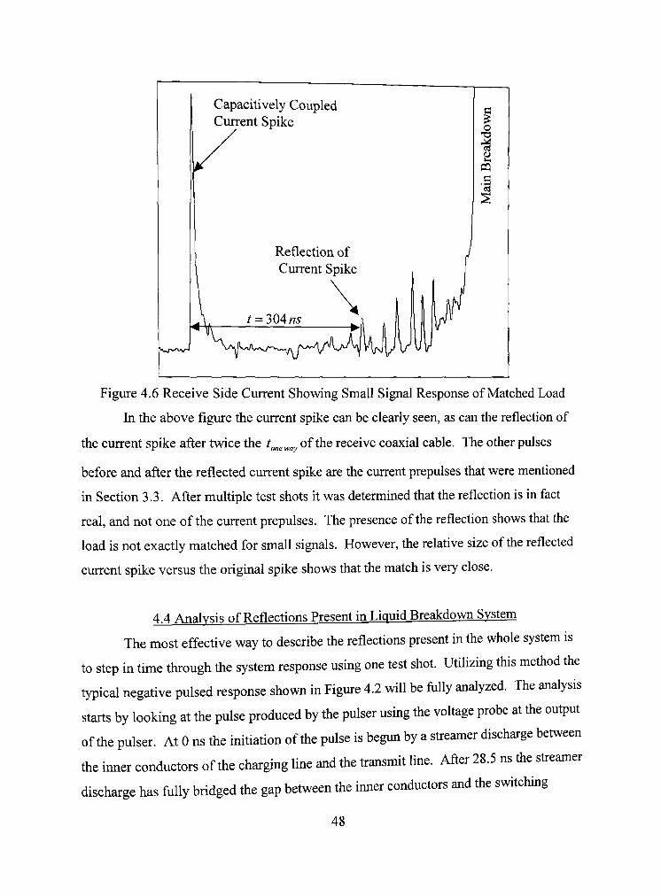
Capacitively Coupled Current Spike
o X)
(U
CQ
Reflection of Current Spike
S-.T'^^^^
Figure 4.6 Receive Side Current Showing Small Signal Response of Matched Load
In the above figure the current spike can be clearly seen, as can the reflection of
the current spike after twice the t^„^„^ of the receive coaxial cable. The other pulses
before and after the reflected current spike are the current prepulses that were mentioned
in Section 3.3. After multiple test shots it was determined that the reflection is in fact
real, and not one of the current prepulses. The presence of the reflection shows that the
load is not exactly matched for small signals. However, the relative size of tiie reflected
current spike versus the original spike shows that the match is very close.
4.4 Analvsis of Reflections Present in Liquid Breakdown Svstem
The most effective way to describe the reflections present in the whole system is
to step in time through the system response using one test shot. Utilizing this metiiod the
typical negative pulsed response shown in Figure 4.2 will be fiilly analyzed. The analysis
starts by looking at the pulse produced by the pulser using the voltage probe at the output
of the pulser. At 0 ns the initiation of the pulse is begun by a streamer discharge between
the imier conductors of the charging line and the tiansmit line. After 28.5 ns the streamer
discharge has fiilly bridged the gap between the imier conductors and the switching
48

action is complete. This initiates a negatively rising edge that tiavels down the transmit
line toward the main chamber, and a positively rising edge that tiavels down the charging
line toward the charging resistor. Once the rising edge on the tiansmit line reaches the
main chamber a reflection is caused by the chamber. This reflected rising edge travels
from the chamber back to the switch. This reflection is seen at the switch 306 ns after the
pulse has left the pulser. From the peak of this pulse the reflection coefficient of the
chamber without a discharge present is calculated as 0.979. At some point in time the
presence of the high voltage on the transmit side of the chamber causes a streamer
discharge to bridge the gap inside the main chamber and connect the inner conductor of
the transmit line to the inner conductor of the receive line. In the test shown in Figure 4.2
it takes 175 ns for this breakdown to occur. All of this is illustrated in Figure 4.7 below.
I D) B >
0
-10
-20
-30
-40
-50
-60
-70
-80
-90
-iqcj
306 m . \15ns ^
Peak at 47 kV
Rises to 93 kV
-Fall of 53 kV-
00 100 500 600 700 200 300 400 Time [ns]
Figure 4.7 First 700 ns from the Spark Gap Voltage Probe
Once the breakdown in the main chamber occurs a negatively rising edge travels
down the receive line to the matched load, and a positively rising edge travels down the
transmit line going toward the switch. The positively rising edge causes the larger falling
edge seen in Figure 4.7 at 481 ns. At 705 ns the falling edge from the pulser arrives at
49

the vohage probe and stops the main pulse of the pulser. The smaller fall time associated
with this pulse is due to tiie transmission coefficient of the impedance mismatch at the
switch. Three hundred and six nanoseconds after the falling edge of the main pulse a
secondary pulse arrives at the voltage probe. The secondary pulse is a result of the pulse
created by the mismatch at the main chamber moving down the charging line, being
reflected by the charging resistor and coming back through the spark gap. At this point in
time the streamer discharge has not had enough time to fully close and so the secondary
pulse passes through. In fact the secondary pulse will travel all the way to the matched
load due to a persisting streamer discharge inside the main chamber. This can be seen in
the receive voltage signal in Figure 4.2. The falling edge of the pulse and the secondary
pulse as seen from the spark gap voltage probe are shown in Figure 4.8. 20 r
I B "o >
900 1000 1100 I UU 1300
Time [ns]
Figure 4.8 Next 600 ns from the Spark Gap Voltage Probe
The falling edge of the main pulse, and the secondary pulse travel all the way
through the system, hi the process they produce reflections at each of the impedance
mismatches shown in Figure 4.1. This results in a negative going pulse and a positive
going edge that are reflected at several points in the system. These smaller wavefomis
bounce around in the system until both streamer discharges have stopped, resulting m the
50

smaller reflections seen in all of the waveforms in Figure 4.2. Analysis of the individual
smaller reflections recorded by a particular voltage probe is difficult due to the addition
of the two waveforms and the multiple reflections that ensue from the three impedance
mismatches. In addition, the collapsing streamer discharges in both the main chamber
and the spark gap causes a changing reflection coefficient in each. This magnifies the
problem of analyzing the smaller reflections since the status of the streamer discharges
cannot be measured after the end of the main pulse. However, the genesis of the smaller
reflections is clear from the analysis of the pulses previous to 1300 ns.
51

CHAPTER V
CONCLUSION
A high voltage charged line pulser system has been created for liquid breakdown
testing at the Center for Pulsed Power and Power Electronics. The pulser produces an
output pulse of 60kV into a matched 50Q load and a 120kV output pulse into an open
load, with a charging voltage of 120kV. The pulser can be charged with either a positive
or a negative polarity. The FWHM pulse length of the pulser is 706ns and the average
rise time is 20ns. The pulser utilizes a liquid switching medium coaxial spark gap and an
RG-220 charging cable to produce the output pulse. In addition to the pulser, a
50 Q matched load has been constructed and tested for a 60 kV pulse.
52

REFERENCES
1] Cheng, David K. Field and Wave Electromagnetics Second Edition; New York: Addison-Wesley Publishing Company, 1992, p 427-440.
2] A Short Course in Pulsed Power, prepared by the faculty at the Center for Pulsed Power and Power Electionics, 2003, p 15.
3] Martin, J.C. Solid, Liquid and Gaseous Switches: AF Pulsed Power Lecture Series No. 30; Texas Tech University, Lubbock, TX; 1981, p 56, 287-293.
4] Pai, S. T. and Zhang, Qi. Introduction to High Power Pulse Technology; River Edge, New Jersey: World Scientific Pubhshing Company, 1995, p 59-61, 173-176.
5] Nasser, Essam. Fundamentals of Gaseous Ionization and Plasma Electronics; New York: Wiley-hiterscience, 1970, p 251-277.
6] Hemmert, H., et. al. Optical Diagnostics of Shock Waves Generated by a Pulsed Streamer Discharge in Water; Presented at the 14* IEEE International Pulsed Power Conference, Dallas, TX, June, 2003.
7] Times Microwave Website accessible at www.timesmicrowave.com.
8] Hatfield, L. L. September 26*, 2003, Personnel Communication, Department of Physics, Texas Tech University, Lubbock, TX.
53

PERMISSION TO COPY
In presenting this thesis in partial fiilfillment of tiie requirements for a
master's degree at Texas Tech University or Texas Tech University Healtii Sciences
Center, I agree that the Library and my major department shall make it freely
available for research purposes. Permission to copy this thesis for scholarly purposes
may be granted by the Director of the Library or my major professor. It is
understood that any copying or publication of this thesis for financial gain shall not
be allowed without my further written permission and that any user may be liable for
copyright infringement.
Agree (Permission is granted.)
Student Signature Date
Disagree (Permission is not granted.)
Student Signature Date