ARTICLEShttps://doi.org/10.1038/s41587-021-00986-5

1Center for Integrative Imaging, Hefei National Laboratory for Physical Sciences at the Microscale, and School of Life Sciences, University of Science and Technology of China, Hefei, China. 2CAS Key Laboratory of Brain Connectome and Manipulation, Interdisciplinary Center for Brain Information, The Brain Cognition and Brain Disease Institute, Shenzhen Institute of Advanced Technology, Chinese Academy of Sciences; Shenzhen-Hong Kong Institute of Brain Science-Shenzhen Fundamental Research Institutions, Shenzhen, China. 3CAS Key Laboratory of Brain Function and Disease, and School of Life Sciences, University of Science and Technology of China, Hefei, China. 4Key Laboratory of Animal Models and Human Disease Mechanism, Kunming Institute of Zoology, Chinese Academy of Sciences, Kunming, China. 5Department of Pathology and Pathophysiology, Kunming Medical University, Kunming, China. 6Institute of Artificial Intelligence, Hefei Comprehensive National Science Center, Hefei, China. 7McGovern Institute for Brain Research, Massachusetts Institute of Technology, Cambridge, MA, USA. 8State Key Laboratory of Magnetic Resonance and Atomic and Molecular Physics, Key Laboratory of Magnetic Resonance in Biological Systems, Wuhan Institute of Physics and Mathematics, Chinese Academy of Sciences, Wuhan, China. 9Zilkha Neurogenetic Institute, Center for Neural Circuits & Sensory Processing Disorders, Keck School of Medicine, University of Southern California, Los Angeles, CA, USA. 10UCLA Brain Research & Artificial Intelligence Nexus, Department of Neurobiology, David Geffen School of Medicine, University of California Los Angeles, Los Angeles, CA, USA. 11CAS Center for Excellence in Brain Science and Intelligence Technology, Shanghai, China. 12These authors contributed equally: Fang Xu, Yan Shen, Lufeng Ding, Chao-Yu Yang. ✉e-mail: plau@ustc.edu.cn; gqbi@ustc.edu.cn

Given the status of nonhuman primates, including the rhesus macaque (Macaca mulatta), as important experimental ani-mals for modeling of human cognitive functions and brain

diseases1,2, a fundamental task in neuroscience and neurology is mapping structural connectivity among different brain regions and neurons (that is, the mesoscopic connectome) of the monkey brain, preferably at subcellular resolution3–7, in a way similar to that established for the mouse brain. Structural connectivity mapping of nonhuman primate brains has, to date, relied primarily on bulk labeling of specific brain regions with antero- and retrograde trac-ers, followed by interleaved two-dimensional light microscopy of serial thin sections8–10. This neurohistological approach provides an elaborate view of brain sections at micron or submicron resolution. However, the axial spatial resolution of this approach is limited by the sectioning thickness (usually ~20–120 µm) and sampling ratio of sections (usually ~1/6–1/3), and thus lacks the resolution and con-tinuity necessary for tracking of individual neurites across slices11.

Widely used tractography approaches based on diffusion-weighted magnetic resonance imaging are able to image the entire monkey or human brain as a whole, but their anatomical accuracy is inherently limited12–15. Light-sheet microscopy combined with whole-brain clearing techniques can image intact mouse brains, but lacks the resolution to distinguish individual axons16–21. Recently developed

block-face imaging techniques22–26, including serial two-photon tomography22,23,25 and fluorescence micro-optical sectioning tomog-raphy24, have successfully implemented brain-wide axonal tracing in mice and have ushered in a new era of connectomic mapping27,28. However, given that these techniques usually require several days to image a mouse brain, it is very difficult to scale them up toward sys-tematic connectomic mapping for much larger macaque or human brains (Supplementary Table 1).

To overcome these technical bottlenecks, we developed an inte-grative approach consisting of serial sectioning of the brain tissue into thick slices, clearing with primate-optimized uniform clear-ing solutions, fluorescence imaging based on the synchronized on-the-fly-scan and readout (VISoR) technique29 with improve-ments for ultrahigh-speed microscopy of large slices, and a semiau-tomated process for volume reconstruction and axonal tracing. This SMART strategy and pipeline (Fig. 1a), due to its high throughput and scalability, overcame several key technical challenges to enable high-resolution mapping of the entire macaque brain. We gener-ated a projection map from viral-labeled thalamic neurons to the cerebral cortex and unveiled distinct axonal routing patterns in the folded banks along the superior temporal sulcus (STS), and carried out efficient semiautomated tracing of neuronal fibers through the near-petabyte dataset of the monkey brain.

High-throughput mapping of a whole rhesus monkey brain at micrometer resolution

Fang Xu   1,2,12, Yan Shen3,12, Lufeng Ding3,12, Chao-Yu Yang3,12, Heng Tan4,5, Hao Wang1,6, Qingyuan Zhu1,

Rui Xu   7, Fengyi Wu2, Yanyang Xiao   2, Cheng Xu1, Qianwei Li1, Peng Su8, Li I. Zhang9,

Hong-Wei Dong10, Robert Desimone7, Fuqiang Xu2,8,11, Xintian Hu4,11, Pak-Ming Lau   1,2,3,6 ✉ and

Guo-Qiang Bi   1,2,6,11 ✉

Whole-brain mesoscale mapping in primates has been hindered by large brain sizes and the relatively low throughput of avail-able microscopy methods. Here, we present an approach that combines primate-optimized tissue sectioning and clearing with ultrahigh-speed fluorescence microscopy implementing improved volumetric imaging with synchronized on-the-fly-scan and readout technique, and is capable of completing whole-brain imaging of a rhesus monkey at 1 × 1 × 2.5 µm3 voxel resolution within 100 h. We also developed a highly efficient method for long-range tracing of sparse axonal fibers in datasets numbering hundreds of terabytes. This pipeline, which we call serial sectioning and clearing, three-dimensional microscopy with semi-automated reconstruction and tracing (SMART), enables effective connectome-scale mapping of large primate brains. With SMART, we were able to construct a cortical projection map of the mediodorsal nucleus of the thalamus and identify distinct turning and routing patterns of individual axons in the cortical folds while approaching their arborization destinations.

NaTuRe BIoTeCHNoLoGY | www.nature.com/naturebiotechnology

ARTICLES NATURE BIOTECHNOLOGY

AAV9-CreAAV9-DIO-FP

Macaque brain Serial sectioning and clearing VISoR2 microscopy Semiautomated

Reconstruction Tracing

Opaque

Cleared

Nissl

DAPI

Nissl

DAPI

SDS + RIMS PuClear0

150

300

Depth

(µm

)

Camera

Sample

Stages

Rolli

ng

Chip

Sync

Scanner

Lasers

FocalplaneScan

Rigid

12

...Stack no.

n – 1

n

Slic

e n

o.

......

Nonrigid

y

x

z

y

Intraslice stitching error (µm) Interslice stitching error (µm)

Pro

babili

ty

0.4

0.2

00 2 4 6 8

x

y

z

Pro

babili

ty

0 10 20 30 40

0.4

0.2

0

x

y

z

z = 0 µm

z = 3 µm

z = 8 µm

z = 0 µm

z = 3 µm

z = 8 µm

eGFP

mCherry

DAPI

eGFP

mCherry

Nissl

eGFP

mCherry

Nissl

a

b

e

c d

f

i j k

g h

l m n

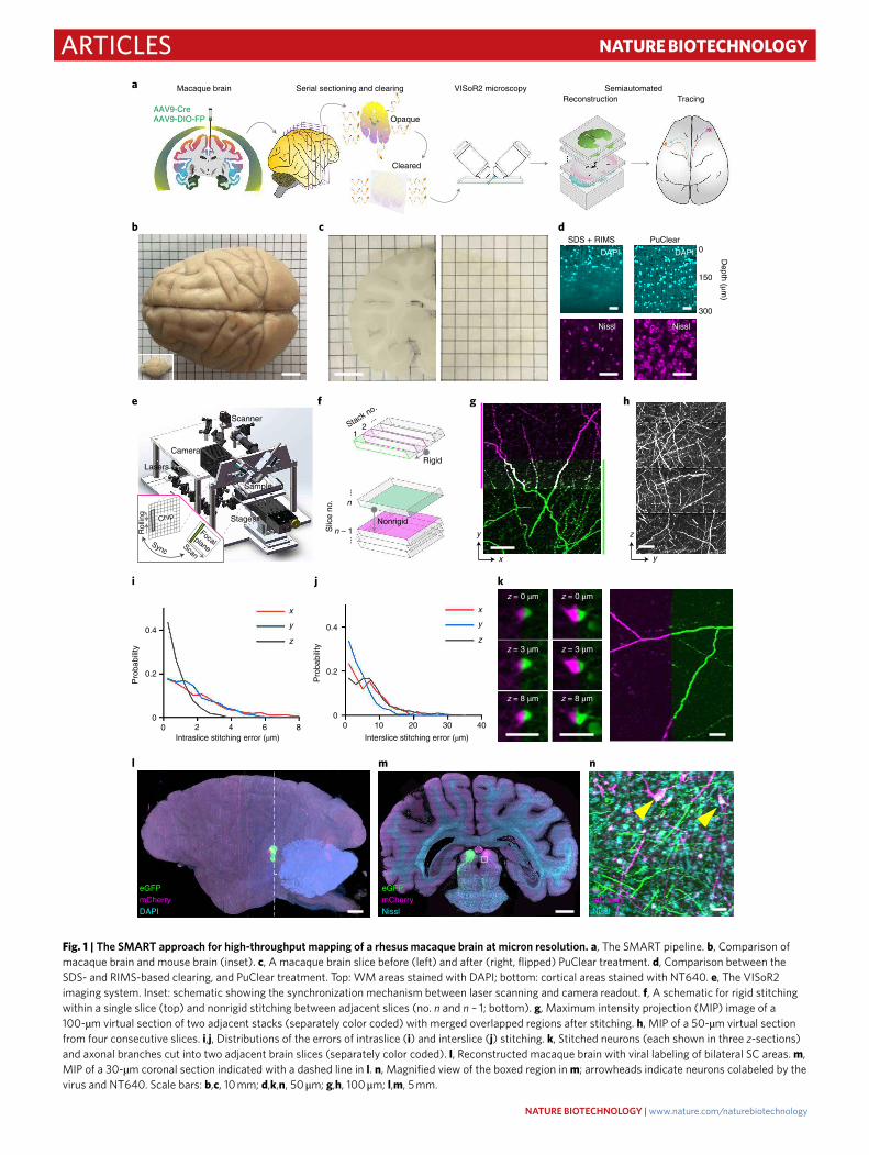
Fig. 1 | The SMaRT approach for high-throughput mapping of a rhesus macaque brain at micron resolution. a, The SMART pipeline. b, Comparison of

macaque brain and mouse brain (inset). c, A macaque brain slice before (left) and after (right, flipped) PuClear treatment. d, Comparison between the

SDS- and RIMS-based clearing, and PuClear treatment. Top: WM areas stained with DAPI; bottom: cortical areas stained with NT640. e, The VISoR2

imaging system. Inset: schematic showing the synchronization mechanism between laser scanning and camera readout. f, A schematic for rigid stitching

within a single slice (top) and nonrigid stitching between adjacent slices (no. n and n – 1; bottom). g, Maximum intensity projection (MIP) image of a

100-µm virtual section of two adjacent stacks (separately color coded) with merged overlapped regions after stitching. h, MIP of a 50-µm virtual section

from four consecutive slices. i,j, Distributions of the errors of intraslice (i) and interslice (j) stitching. k, Stitched neurons (each shown in three z-sections)

and axonal branches cut into two adjacent brain slices (separately color coded). l, Reconstructed macaque brain with viral labeling of bilateral SC areas. m,

MIP of a 30-µm coronal section indicated with a dashed line in l. n, Magnified view of the boxed region in m; arrowheads indicate neurons colabeled by the

virus and NT640. Scale bars: b,c, 10 mm; d,k,n, 50 μm; g,h, 100 μm; l,m, 5 mm.

NaTuRe BIoTeCHNoLoGY | www.nature.com/naturebiotechnology

ARTICLESNATURE BIOTECHNOLOGY

ResultsSection clearing and VISoR2 imaging of the macaque brain. The first major challenge in regard to imaging of large brains is sample preparation. The difficulty of reagent penetration increases exponentially with tissue thickness, making it exceedingly dif-ficult to achieve uniform histological staining or clearing of the whole monkey brain, which is >200 times larger than a mouse brain (Fig. 1b)10. We therefore chose to section the brain into slices before subsequent clearing and imaging. A robust workflow was established with hydrogel-based embedding to minimize tissue loss and distortion during sectioning and clearing (Supplementary Figs. 1 and 2 and Methods). A macaque brain was sectioned into about 250 consecutive 300-µm slices, which were treated with a primate-optimized uniform clearing method (PuClear) that com-bines Triton X-100-based gentle membrane permeabilization with high refractive index matching (Fig. 1c). Unlike the widely used clearing methods based on delipidation with sodium dodecyl sul-fate (SDS) and the refractive index matching solution (RIMS) with a refractive index of ~1.46 (refs.16,17,29), which we found inadequate for clear imaging through the white matter (WM) of primate tissue, PuClear has a matching refractive index of 1.52 yielding uniform transparency through the full depth of 300-µm slices, including WM areas (Fig. 1d, top). PuClear preserved the morphology of neu-rons labeled by Nissl staining (Fig. 1d, bottom) and showed excel-lent compatibility with both immunostaining for cell visualization (Supplementary Fig. 3) and cholera toxin subunit B (CTB) labeling for retrograde tracing (Supplementary Fig. 4).

Uniform clearing of thick brain slices also allowed us to over-come a second major challenge, the long duration required for imaging of a large brain at high resolution. For this, we developed an improved version of our recently reported VISoR technique29. This VISoR2 system is optimized for ultrahigh-speed volumetric imaging of larger monkey brain sections (Fig. 1e). Besides instru-mental upgrades, including long-travel linear stages and a more compact and stable light path, the system was implemented with an optimized control sequence for the scientific complementary metal oxide semiconductor camera, the illumination laser and the galva-nometer scanner (Supplementary Fig. 5; Methods).

We achieved 250-Hz, blur-free imaging of a 0.7 × 2.0 mm2 field of view containing the optical section of the slice, with smooth stage movement at any speed ranging from 0.5 to 20 mm s–1. This configu-ration corresponds to a voxel resolution of 1.0 × 1.0 × (~1.4–56) µm3 and a continuous data rate of 400 million voxels s–1 (Supplementary Fig. 5 and Supplementary Video 1). Thus the system is capable of imaging a mouse brain that is serially sectioned, cleared and mounted on a single glass slide within 30 min at 1.0 × 1.0 × 2.5-µm3 resolution. Consequently, the collection of ~80 million single-channel images (2,048 × 788 pixels each) for all slices from one macaque brain required only 94 h of imaging time. VISoR2-based imaging across three channels resulted in 750 terabytes (TB) of data for a rhesus macaque brain that was labeled by coinjection of adeno-associated virus (AAV) cocktails, mixed by an AAV carrying Cre recombinase and another AAV carrying a Cre-dependent fluorescent protein (FP) reporter, either enhanced green fluorescent protein (eGFP) or mCherry, into the left and right superior colliculus (SC), respec-tively. Compared to the latest neurohistological pipeline that com-pleted mapping of a whole marmoset brain in 2 weeks with 8 TB of data collected10, our approach shows an improvement of ~20–100-fold in imaging throughput (Supplementary Table 1).

Reconstruction of the entire macaque brain. While VISoR2 microscopy with substantially improved imaging speed overcame the second challenge in primate brain mapping, it generated a third: the analysis of such a large dataset. Available tools have been effec-tive in handling TB-level, multitile images, but these tools either cannot be used for nonoverlapped image tiles30,31 or lack automation

for multihundred-TB data32. We therefore developed a custom software tool that implements automated volume stitching (Fig. 1f and Supplementary Fig. 6), including rigid-transformation-based three-dimensional (3D) intraslice stitching (Fig. 1g) and nonrigid-transformation-based interslice alignment (Fig. 1h and Supplementary Video 2). Attesting to the strong performance of this tool we found that, for each axis, intraslice stitching errors were ~2 µm (Fig. 1i) and the interslice alignment error of AAV-labeled axons was ~6–8 µm (Fig. 1j). Tissue loss between consecutively sec-tioned slices was minor, as seen in the precise alignment of trun-cated cell bodies and axonal branches (Fig. 1k). As we demonstrate below, this precision was sufficient for visual tracing of axonal pro-jections. In practice, we reconstructed the whole brain at a coarse voxel resolution (10 × 10 × 10 µm3) to obtain an overview of brain structures and also established a robust transformation framework for on-demand reconstruction of user-specified regions of interest (ROIs) at full resolution for detailed analysis of axonal projections (Fig. 1l–n and Supplementary Fig. 7).

Mesoscopic mapping of thalamocortical projection. To dem-onstrate the capacity of our system for mesoscopic mapping of neuronal projections across the entire monkey brain, we bilater-ally injected AAV cocktails into the left and right medial dorsal nucleus of the thalamus (MD), with minor leakage to nearby areas (Supplementary Fig. 8). The MD is known to generate dense projec-tions to the prefrontal cortex (PFC)33,34. VISoR2 imaging and 3D reconstruction of this monkey brain allowed for visualization of the global distribution of axons originating from the injection sites and projecting into the cerebral cortex (Fig. 2a). From the 3D vol-ume and a series of virtual sections, it was clear that bundled fibers from the injection sites traveled through the internal capsule (IC) in horizontal, obliquely lateral and upward directions (Fig. 2b,c and Supplementary Video 3) before continuing on towards the frontal lobe, where they primarily targeted the posterior orbitofrontal area (Fig. 2d and Supplementary Fig. 9), largely consistent with previous reports of MD projections33,35. Furthermore, the resolution of the original images was sufficient for us to visualize individual axons and branches when label density was not too high, and to distin-guish whether the fibers were passing by or making terminal arbori-zations based on 3D visualization of the volume images (Fig. 2e–h). For instance, our PFC mapping revealed that labeled axons termi-nate in layers III and IV (Fig. 2g,h and Supplementary Video 4). Besides the canonical target areas of the MD in the ipsilateral PFC with high-density arborizations of labeled axons, we also observed various lower-density, yet notable, fiber branches and arboriza-tions in other areas such as the ipsilateral secondary somatosensory cortex (SII) (Fig. 2i,j), which is known to be a target of the ventral posterior inferior nucleus and ventral posterolateral nucleus36, and the temporal lobe, including STS dorsal (TPO) and ventral (TEa) bank areas (Fig. 2k,l and Supplementary Fig. 9). All projection tar-gets observed in this animal are summarized in Supplementary Table 2 and visualized in Fig. 2m in a cortical map after flattening (Supplementary Fig. 10). Thus, the high resolution and sensitivity of SMART imaging may help reveal previously unidentified cortical targets of the MD, although some of these observations could be due to inadvertent labeling of neurons in other nuclei close to the injection sites. More precise injection or a sparse labeling approach that allows complete single-neuron tracing will help resolve such uncertainties and unveil detailed thalamocortical projection maps.

Distinct patterns of axonal routing in cortical folds. The resolution of our system also allowed for identification of fine features of indi-vidual axonal segments in the projection sites where fibers were not excessively dense. As an example, we reconstructed a full-resolution volume of areas near the STS and traced 30 randomly selected axo-nal segments (Fig. 3a,b and Supplementary Video 5) using custom

NaTuRe BIoTeCHNoLoGY | www.nature.com/naturebiotechnology

ARTICLES NATURE BIOTECHNOLOGY

tracing software. In these folded areas, axons projecting to layers III/IV of the TEa typically navigated to the dorsal side first before sep-arating into two major groups—one group made sharp turns in the WM (Fig. 3c, top), traveling along the boundary of the WM

(Fig. 3c, bottom), while the other made right-angle turns and trav-eled through the superficial cortical layers (Fig. 3d). We observed four distinct classes of turning pattern for these axons (Fig. 3e–h). Such differences in the micro-organization of these afferent axons

eGFP (high)

eGFP (low)

mCherry

23c

23b23a

TEpv

RM

Pir

TPO

PGa

TAa

IPaTEa

TEm

F3F2

7op

7b

7a

LIPd

Tpt

Iam

IaiIal

Iapl

GPrCO

Id

SIIIg

Iapm

8Av45b

45a46v

12r12m

12l

13b13m

13l

13a

12o

44

F5

F4

46d

11l

46f

8Ad

25

32

24a24b

10mc

24c

10mr

10o

9m9d

8Bm

8BdF6

F78Bs

11m

(d) (i)eGFP

mCherryx

y

a

p

i

sl

r

(c)

1 mm

z

y

x

13b

eGFPmCherry

(e)

(g)

(h)

(f)

300

0

III

III

IV

V/VI

180

150

(k)

(j)

STS

LS

eGFPmCherry

SII

Insula

TEa

IPa

TPO

(l)

TPO

a b c

d e f g h

i j

k

l

m

Fig. 2 | Mesoscopic mapping of the MD projection. a, Reconstructed macaque brain with viral labeling of bilateral MD areas. b–c, Fiber orientation

image of the brain (b) and magnified view of the left IC (c). Only the eGFP channel is displayed, where red, green and blue represent the left/right,

superior/inferior and anterior/posterior orientations, respectively. d, MIP of an example 300-μm coronal section showing the prefrontal projection of the

MD. e, Enlargement of the boxed region in d, in which the blue–green–yellow–orange spectrum encodes the depth (in μm). Cortical layers are outlined

based on autofluorescence patterns in the mCherry channel (magenta). f, Magnified view of boxed region in e, showing a representative passing axon

(arrowhead) covering the full depth spectrum. g,h, Magnified views of boxed regions in e, showing typical arborized axon terminals (arrowheads) ending

in the mid-depth of layer III (g) or layer IV (h) of the slice. The spectrum codes a depth range of ~0–300-μm in e–g and ~150–180 μm in h. i–l, MIP of a

300-μm coronal section (i), with magnified views showing projections to the SII (j) and temporal lobe (k, zoomed-in view in l). m, Summarized cortical

flat map showing high- and low-density distribution of axonal projections to the ipsilateral hemisphere from the injection sites, as revealed by eGFP and

mCherry expression. Scale bars: a,b,d,i, 5 mm; e, 200 μm; f–h, 50 μm; j, 1 mm; k, 500 μm; l, 100 μm. LS, lateral sulcus; other anatomical sites are listed in

Supplementary Table 2.

NaTuRe BIoTeCHNoLoGY | www.nature.com/naturebiotechnology

ARTICLESNATURE BIOTECHNOLOGY

may underlie their functional diversity, especially when they make putative en route connections with different sets of neurons posi-tioned within various local circuits.

Brain-wide tracing of individual axons. With the capacity of resolving individual axonal segments, we set out to trace the long-range projections of some sparsely labeled macaque axons

90°

eGFP

Autofluorescence

Axon tracing

eGFP

Autofluorescence

Axon tracing

TEa

TPO

WM

STSSTS STS STSTEa

TPO

WM

TEa

TPO

WM

TEa

TPO

WM

a b

c

e f g h

d

Fig. 3 | organization of axonal fibers in cortical folds. a, Overview of a 16 × 11 × 11-mm3 image volume surrounding the STS from an

MD-injected macaque. b, Thirty traced axonal segments shown from two perspectives. Curved brain surfaces were segmented and rendered as a

shaded reference to help visualize the location of axon trajectories. c, Example images showing the sharp turns (arrowheads) of five axons

(top) in the WM and the arbor area of an axon (bottom). d, Example images showing the right-angle turns (arrowheads) of an axon (top) and

its arbors (bottom). Images in the top panels of c,d are MIPs of 450-µm virtual sections resliced in an orientation parallel to the fibers. The bottom

images in c,d are MIPs of 1,200-µm sections. e–h, Four axonal navigation patterns: those following short paths (e), those making sharp turns

(f), those making two-step, right-angle turns (g) and those making right-angle turns (h). The boundaries of cortical surfaces are illustrated as

solid lines while those of the WM are illustrated as dashed lines. Cortical layer IV can be recognized as a dim band in the autofluorescence images,

and is drawn with dotted lines. Fibers shown in c,d are highlighted in f,g, respectively, but are presented in different perspectives. Scale bars: a,b,e–h,

2 mm; c,d, 200 μm.

NaTuRe BIoTeCHNoLoGY | www.nature.com/naturebiotechnology

ARTICLES NATURE BIOTECHNOLOGY

but encountered yet another challenge. Whereas convenient tools have been developed for brain-wide tracing of single neurons in the mouse27,37–39, these tools work with full-resolution stitched datasets, which require additional storage and heavy computation costs. For example, full-resolution fusion of a 1.67-TB dataset requires ~24 h computation on a high-performance workstation31. If this scales up linearly to our 750-TB macaque dataset, it would take more than a year. In addition, the reconstructed local image is often of somewhat lower quality than the raw image, partly because of errors intro-duced by nonlinear deformation and interpolation steps imple-mented to achieve global consistency. Therefore, we developed a computationally efficient strategy for progressive tracing of axons by dynamically loading only blocks of necessary raw images. For this, we first generated a relatively low-resolution (10 × 10 × 10 μm3) reconstruction volume of the macaque brain and established a

‘SMART positioning system’ (SPS) that employs a set of bidirec-tional transformations to enable mapping between the initially defined whole-brain coordinate system and the corresponding data from each raw image (Fig. 4a).

An iterative workflow was then established to trace the rela-tively sparsely labeled axons projecting to the contralateral hemi-sphere (Fig. 4b). In this scheme, bright fiber trunks were first identified in the low-resolution whole-brain image followed by semiautomated tracing in full-resolution raw image blocks that were dynamically loaded as tracing progressed along the axon track; this process proceeded until reaching either the injection site (where the fibers were too dense) (Fig. 4c) or the nerve end-ing of each axonal branch (Fig. 4d). The speed of semiautomated tracing approached ~10–30 mm h–1, which is close to that of meth-odologies for the rodent dataset27, depending on the signal/noise

Raw image stacks

(OME-TIFF format)

SPS

Reconstructed

brain volume

(IMS format)

Level n

Level n – 1

Level 0

…

P(s,k,xr,yr,zr)

Affine and nonrigid

transformations

Pʹ(xv,yv,zv)

SPS

SPS * 2SPS

1. Low-res. brain 2. Seeding 3. Locate to raw stack

4. Semiauto. tracing

5. Locate to the next slice

6. Progressive tracing7. Complete

SMART tracing

MD

RE

(d)

(f)

(c)

a

p

rl

a

b

c d f

e

Fig. 4 | Brain-wide tracing of axonal projections. a, SPS maps between any position P located at (xr, yr, zr) in a raw image stack (k) of a brain slice (s) and

the corresponding point P′(xv, yv, zv) in the space of the reconstructed brain volume. b, Step-by-step workflow for SMART-based axonal tracing. Starting

from a low-resolution (res) image (b1), a seed node was selected (b2) and located via SPS in the raw image stack (b3); subsequent semiautomated

(semiauto) tracing was conducted (b4) to navigate through to the edge of the slice and beyond into the neighboring zone of the adjacent slice as identified

by SPS (b5). The entire axon could then be traced by iteratively applying steps 4 and 5 (b6), and finally visualized in the reconstructed brain space by

reverse transformation of traced coordinates via SPS (b7). c,d, Tracing was terminated either at the injection site where the axons were too dense (c) or

at axonal termini (d). Arrowheads denote typical nerve endings. e, Six thalamocortical axons projecting into the right hemisphere from the left MD or RE

areas. f, Magnified view of clustered axonal terminals overlapped with a raw image block. Scale bars: c, 20 μm; d, 10 μm; e, 5 mm; f, 500 μm.

NaTuRe BIoTeCHNoLoGY | www.nature.com/naturebiotechnology

ARTICLESNATURE BIOTECHNOLOGY

ratio in different areas and the proficiency of annotators. When necessary, any misalignment between adjacent slices from errors in the automated registration process was manually corrected based on the continuity of foreground neuronal fibers and back-ground microvasculature (Supplementary Fig. 11). By this means, interslice stitching precision can be refined during the manual tracing process as annotations increase. For example, the lateral accuracy in surrounding area of a traced axon was improved from 7.5 ± 4.4 to 4.8 ± 3.3 µm after two annotation pairs were labeled at each cut surface between slices (n = 68, mean ± standard devia-tion, P = 0.0001, paired t-test) (Methods).

Using this progressive SMART tracing strategy, we tracked back 28 randomly selected bright fiber trunks retrogradely to the injec-tion site and anterogradely to their branching points. These fibers travel in parallel in a bundle within the internal capsule before branching out into divergent cortical areas (Supplementary Fig. 12; distances before branching: 26.8 ± 1.6 mm, n = 28). We also selected six of these fiber trunks and mapped out their full terminal arboriza-tions (Fig. 4e and Supplementary Video 6). For tracing of each axon, only ~1.7% of raw images were sequentially accessed (total size of the raw images: 238 TB; size of images accessed during tracing: 4.1 ± 1.2 TB, n = 6), with multiple image blocks of ~2–256 megabytes (~128 × 128 × 128 to 1,024 × 1,024 × 256 voxels each) loaded into memory at a time, a workload manageable by a personal computer. Notably, most of these axonal fibers form clustered arborizations in confined cortical regions (Fig. 4f), with negligible subcortical arborizations (3.4 ± 2.6% of total axonal length, n = 6), in striking contrast to the previously mapped mouse thalamic projections from the MD and nearby reunions nucleus (RE) (Supplementary Fig. 13 and Supplementary Table 3).

DiscussionOwing to its implementation of optimized tissue slicing and clearing, ultrahigh-speed imaging techniques and efficient analysis tools for processing of near-petabyte-scale datasets, SMART bridges the gap in our understanding of functionally impactful differences between rodent and human brain architectures, specifically by enabling the efficient mapping of primate brains at subcellular resolution and supporting brain-wide, long-range tracing of sparse axons. Indeed, our proof-of-concept study has already begun to reveal potential new targets of primate thalamocortical projections and to highlight distinct properties of individual axons, including their long trunks and striking turning patterns as they progress towards cortical tar-gets. Although this initial study allowed for tracing of only a small number of single fibers, mainly because of the very dense labeling and relatively low throughput of semiautomated axonal tracing, much sparser labeling is achievable by lowering the concentration of Cre recombinase-carrying AAV in the viral injection cocktail40,41. By adapting the progressive brain-wide tracing strategy provided by our custom software, Lychnis (Methods), that already achieves a tracing speed comparable to that of previous studies in mice27, together with newly developed high-performance computing and automation techniques39,42, it is expected that the SMART system will allow for mapping of the full morphology of a potentially huge number of individual neurons, thus paving the way toward a truly connectome-scale understanding of the primate brain.

It should also be noted that SMART is compatible with widely used experimental techniques for histological labeling, especially immunofluorescence labeling, which allows for cell-type-specific analysis of the organization of neurons and fibers—for example, the distribution of dopaminergic neurons and their axonal projec-tion patterns (Extended Data Fig. 1). This is particularly important for specimens not amenable to viral labeling—for example, post-mortem human brains43. The strategies underlying SMART, includ-ing nonoverlapped physical slicing and computational stitching, high-throughput blur-free imaging and progressive tracing in raw

image stacks, are all readily scalable and applicable to other biologi-cal samples, including internal organs and even the whole bodies of various species labeled with antero- or retrograde transneuro-nal transporting viruses44. Application of these techniques has the potential to improve understanding of brain architecture and yield high-precision, systems-level insights into the development, basic functions and neurological pathology of the entire nervous system.

online contentAny methods, additional references, Nature Research report-ing summaries, source data, extended data, supplementary infor-mation, acknowledgements, peer review information; details of author contributions and competing interests; and statements of data and code availability are available at https://doi.org/10.1038/s41587-021-00986-5.

Received: 17 September 2020; Accepted: 14 June 2021; Published: xx xx xxxx

References 1. Belmonte, J. C. I. et al. Brains, genes, and primates. Neuron 86, 617–631 (2015). 2. Poo, M.-m et al. China Brain Project: basic neuroscience, brain diseases, and

brain-inspired computing. Neuron 92, 591–596 (2016). 3. Markov, N. T. et al. Cortical high-density counterstream architectures. Science

342, 1238406 (2013). 4. Kleinfeld, D. et al. Large-scale automated histology in the pursuit of

connectomes. J. Neurosci. 31, 16125–16138 (2011). 5. Oh, S. W. et al. A mesoscale connectome of the mouse brain. Nature 508,

207–214 (2014). 6. Wang, X.-J. & Kennedy, H. Brain structure and dynamics across scales: in

search of rules. Curr. Opin. Neurobiol. 37, 92–98 (2016). 7. Zeng, H. Mesoscale connectomics. Curr. Opin. Neurobiol. 50, 154–162 (2018). 8. Felleman, D. J. & Van Essen, D. C. Distributed hierarchical processing in the

primate cerebral cortex. Cereb. Cortex 1, 1–47 (1991). 9. Schmahmann, J. & Pandya, D. Fiber Pathways of the Brain (Oxford Univ.

Press, 2009). 10. Lin, M. K. et al. A high-throughput neurohistological pipeline for brain-wide

mesoscale connectivity mapping of the common marmoset. eLife 8, e40042 (2019).

11. Albanese, A. & Chung, K. Neuroimaging: whole-brain imaging reaches new heights (and lengths). eLife 5, e13367 (2016).

12. Jones, D. K., Knösche, T. R. & Turner, R. White matter integrity, fiber count, and other fallacies: the do’s and don’ts of diffusion MRI. Neuroimage 73, 239–254 (2013).

13. Thomas, C. et al. Anatomical accuracy of brain connections derived from diffusion MRI tractography is inherently limited. Proc. Natl Acad. Sci. USA 111, 16574–16579 (2014).

14. Reveley, C. et al. Superficial white matter fiber systems impede detection of long-range cortical connections in diffusion MR tractography. Proc. Natl Acad. Sci. USA 112, E2820–E2828 (2015).

15. Liu, C. et al. A resource for the detailed 3D mapping of white matter pathways in the marmoset brain. Nat. Neurosci. 23, 271–280 (2020).

16. Chung, K. et al. Structural and molecular interrogation of intact biological systems. Nature 497, 332–337 (2013).

17. Yang, B. et al. Single-cell phenotyping within transparent intact tissue through whole-body clearing. Cell 158, 945–958 (2014).

18. Susaki, E. A. et al. Whole-brain imaging with single-cell resolution using chemical cocktails and computational analysis. Cell 157, 726–739 (2014).

19. Matsumoto, K. et al. Advanced CUBIC tissue clearing for whole-organ cell profiling. Nat. Protoc. 14, 3506–3537 (2019).

20. Zhao, S. et al. Cellular and molecular probing of intact human organs. Cell 180, 796–812 (2020).

21. Ueda, H. R. et al. Whole-brain profiling of cells and circuits in mammals by tissue clearing and light-sheet microscopy. Neuron 106, 369–387 (2020).

22. Tsai, P. S. et al. All-optical histology using ultrashort laser pulses. Neuron 39, 27–41 (2003).

23. Ragan, T. et al. Serial two-photon tomography for automated ex vivo mouse brain imaging. Nat. Methods 9, 255–258 (2012).

24. Gong, H. et al. High-throughput dual-colour precision imaging for brain-wide connectome with cytoarchitectonic landmarks at the cellular level. Nat. Commun. 7, 12142 (2016).

25. Economo, M. N. et al. A platform for brain-wide imaging and reconstruction of individual neurons. eLife 5, e10566 (2016).

26. Seiriki, K. et al. High-speed and scalable whole-brain imaging in rodents and primates. Neuron 94, 1085–1100 (2017).

NaTuRe BIoTeCHNoLoGY | www.nature.com/naturebiotechnology

ARTICLES NATURE BIOTECHNOLOGY

27. Winnubst, J. et al. Reconstruction of 1,000 projection neurons reveals new cell types and organization of long-range connectivity in the mouse brain. Cell 179, 268–281 (2019).

28. Peng, H. et al. Brain-wide single neuron reconstruction reveals morphological diversity in molecularly defined striatal, thalamic, cortical and claustral neuron types. Preprint at bioRxiv https://doi.org/10.1101/675280 (2020).

29. Wang, H. et al. Scalable volumetric imaging for ultrahigh-speed brain mapping at synaptic resolution. Natl Sci. Rev. 6, 982–992 (2019).

30. Bria, A. & Iannello, G. TeraStitcher – a tool for fast automatic 3D-stitching of teravoxel-sized microscopy images. BMC Bioinformatics 13, 316 (2012).

31. Hörl, D. et al. BigStitcher: reconstructing high-resolution image datasets of cleared and expanded samples. Nat. Methods 16, 870–874 (2019).

32. Hayworth, K. J. et al. Ultrastructurally smooth thick partitioning and volume stitching for large-scale connectomics. Nat. Methods 12, 319–322 (2015).

33. Ray, J. P. & Price, J. L. The organization of projections from the mediodorsal nucleus of the thalamus to orbital and medial prefrontal cortex in macaque monkeys. J. Comp. Neurol. 337, 1–31 (1993).

34. Parnaudeau, S., Bolkan, S. S. & Kellendonk, C. The mediodorsal thalamus: an essential partner of the prefrontal cortex for cognition. Biol. Psychiatry 83, 648–656 (2018).

35. Giguere, M. & Goldman-Rakic, P. S. Mediodorsal nucleus: areal, laminar, and tangential distribution of afferents and efferents in the frontal lobe of rhesus monkeys. J. Comp. Neurol. 277, 195–213 (1988).

36. Friedman, D. P. & Murray, E. A. Thalamic connectivity of the second somatosensory area and neighboring somatosensory fields of the lateral sulcus of the macaque. J. Comp. Neurol. 252, 348–373 (1986).

37. Bria, A., Iannello, G., Onofri, L. & Peng, H. TeraFly: real-time three-dimensional visualization and annotation of terabytes of multidimensional volumetric images. Nat. Methods 13, 192–194 (2016).

38. Wang, Y. et al. TeraVR empowers precise reconstruction of complete 3-D neuronal morphology in the whole brain. Nat. Commun. 10, 3474 (2019).

39. Gao, R. et al. Cortical column and whole-brain imaging with molecular contrast and nanoscale resolution. Science 363, eaau8302 (2019).

40. Luo, L., Callaway, E. M. & Svoboda, K. Genetic dissection of neural circuits: a decade of progress. Neuron 98, 256–281 (2018).

41. Lin, R. et al. Cell-type-specific and projection-specific brain-wide reconstruction of single neurons. Nat. Methods 15, 1033–1036 (2018).

42. Friedmann, D. et al. Mapping mesoscale axonal projections in the mouse brain using a 3D convolutional network. Proc. Natl Acad. Sci. USA 117, 11068–11075 (2020).

43. Glasser, M. F. et al. A multi-modal parcellation of human cerebral cortex. Nature 536, 171–178 (2016).

44. Levinthal, D. J. & Strick, P. L. Multiple areas of the cerebral cortex influence the stomach. Proc. Natl Acad. Sci. USA 117, 13078–13083 (2020).

Publisher’s note Springer Nature remains neutral with regard to jurisdictional claims in

published maps and institutional affiliations.

© The Author(s), under exclusive licence to Springer Nature America, Inc. 2021

NaTuRe BIoTeCHNoLoGY | www.nature.com/naturebiotechnology

ARTICLESNATURE BIOTECHNOLOGY

MethodsLabeling of viruses. For anterograde neural labeling, recombinant adeno-associated viruses (rAAVs) were generated by transient triple transfection of HEK293 cells, as previously reported45. Cap serotype 9 was chosen to package the AAV vectors to achieve high transduction levels and high titers (>1012 vg ml–1). A strong promoter CAG and transcription control element WPRE were chosen to construct pAAV-CAG-Dio-EGFP-WPRE-pA or pAAV-CAG-Dio-mCherry-WPRE-pA constructs for stable FP expression in primates46. To increase neuronal specificity, we used the hSyn promoter to construct pAAV-hSyn-Cre-WPRE-pA to serve as a controller of FP-expressing vectors.

Mice. Eight-week-old male C57BL/6 and Thy1-YFP-H (Jax: 003782) mice were used in this study for prototyping the sample preparation and imaging methods. All mouse experiments were carried out following protocols approved by the Institutional Animal Care and Use Committees (IACUCs) of the University of Science and Technology of China (no. USTCACUC1601018). All mice used in this study were group housed with a 12/12-h light/dark cycle (lights on at 07.00), controlled temperature (20–22 °C) and humidity (50–70%) and free access to food and water.

Hydrogel monomer solution (HMS, 4%) was prepared for perfusion by mixing 40% (w/v) acrylamide (4% final concentration; no. V900845, Sigma), 2% (w/v) bisacrylamide (0.05% final concentration; no. V3141, Promega), 10× phosphate buffered saline (PBS) (1× final concentration; no. 70011044, ThermoFisher), 8% (w/v) paraformaldehyde (4% final concentration; no. 157-8, Electron Microscopy Sciences), distilled water and VA-044 thermal initiator (0.25% final concentration; no. 223-02112, Wako)16. Perfusion procedures were carried out following a modified protocol based on a previous study29. Mice were deeply anesthetized with 1% sodium pentobarbital solution, followed by transcardial perfusion with 20 ml of 37 °C PBS, 20 ml of ice-cold PBS and, finally, 20 ml of ice-cold 4% HMS. All solutions were perfused at a uniform rate of 10 ml min–1. Mouse brains were harvested and immediately placed in 20 ml of ice-cold 4% HMS and incubated at 4 °C for 24–48 h to allow further diffusion of hydrogel monomers into the tissue.

Monkeys. Three adult, 10-year-old, male rhesus macaques (M. mulatta) were used in this study. Macaques were obtained from breeding colonies of the Primate Research Center of Kunming Institute of Zoology, Chinese Academy of Sciences (KIZ, CAS), which was accredited by the Association for Assessment and Accreditation of Laboratory Animal Care (AAALAC International). The experimental procedures were approved by the IACUC of KIZ, CAS (no. IACUC18018).

To prevent gastric regurgitation caused by anesthesia, fasting and water deprivation were implemented for at least 6 h before surgery. Animals were anesthetized using 10 mg kg–1 ketamine hydrochloride injection intramuscularly (50 mg ml–1, Zhong Mu Bei Kang) and maintained with 20 mg kg–1 pentobarbital sodium intramuscularly (40 mg ml–1, Merck). During surgery, core temperature and heart rate were monitored using a rectal probe and electrocardiograph monitor, respectively. Magnetic resonance imaging (MRI)-assisted brain region positioning was used for accurate encephalic injection, as previously described47. MRI scanning was performed using a 3-T scanner (uMR770, United Imaging) with a 12-channel knee coil. FP-expressing rAAVs (pAAV-CAG-Dio-EGFP-WPRE-pA, 4.70 × 1012 vg ml–1, 2 μl, for the left hemispheres, or pAAV-CAG-Dio-mCherry-WPRE-pA, 3.15 × 1012 vg ml–1, 2 μl, for the right hemispheres) and Cre-expressing rAAVs (pAAV-hSyn-Cre-WPRE-pA, 2.09 × 1012 vg ml–1, 2 μl) were mixed at a 1:1 ratio for each injection. In this study, one macaque was injected with these AAV cocktails in both sides of the SC (AP, −4 mm; ML, ±3 mm; DV, −38 mm) while another was injected with these mixtures in both sides of the MD (AP, 1 mm; ML, ±3 mm; DV, −38 mm). A third monkey was injected with a cholera toxin subunit B-Alexa Fluor 647 conjugate (CTB-AF647; no. C34778, Invitrogen) in the quadrigeminal cistern. Injection duration was >20 min (including 5 min both following insertion and before withdrawal of the microsyringe). Antibiotics were used for 3 days after surgery. Injection sites were further confirmed from reconstructed whole-brain images.

Transcardial perfusions were carried out 8 weeks after surgery. Thirty minutes after anesthesia, each animal was sequentially perfused with the following solutions at the specified speeds: PBS, 8 l (37 °C, 10 ml s–1); PBS, 1 l (4 °C, 1.5 ml s–1); 4% HMS, 1 l (4 °C, 1.5 ml s–1); and 4% HMS, 1 l (4 °C, 0.3 ml s–1). Brains were extracted immediately after perfusion, within 30 min.

Tissue embedding and slicing. A postfixation procedure with hydrogel was set up for crosslinking of proteins and minimization of tissue loss. Immediately after excision, monkey brains were immersed in 500 ml of 4% HMS and stored at 4 °C for 1 week before embedding, to allow penetration of fixatives. Brains were then immersed in the embedding solution, a 1:1 mixture of 4% HMS (2% final concentration) and 20% bovine serum albumin (BSA, 10% final concentration; no. V900933, Sigma), incubated at 4 °C for 1 week, polymerized at 37 °C for 4–5 h and washed three times in PBS to remove residual reagents. Embedding with this mixture of HMS and BSA provides not only in situ fixation of proteins16, but also high material stiffness and toughness for preservation of slice integrity during sectioning (Supplementary Fig. 2). Embedded brains were sectioned into about

250 pieces of 300-µm-thick slices using a vibroslicer (Compresstome VF-800, Precisionary Instruments). All slices of each brain were collected, and each slice was placed in a Petri dish with 40 ml of PBS and stored at 4 °C.

Sample clearing. The PuClear clearing method was established based on the previously reported techniques CLARITY16,17 and CUBIC18 with optimization for primate brain tissues, consisting of membrane permeabilization and refractive index (RI) matching. Brain slices were first treated with a high concentration of Triton X-100 solution (5% in PBS; no. T928, Sigma) for 3–4 days at 37 °C with gentle shaking, to adequately increase membrane permeability, and were then washed with PBS three times. A solution with high RI was prepared by mixing 50 wt% iohexol (no. 29242990.99, Hisyn Pharmaceutical), 23 wt% urea (no. A600148-0002, Sangon), 11 wt% 2,2’,2”,-nitrilotriethanol (no. V900257, Sigma) and 16 wt% distilled water; the final RI of the PuClear RI-matching solution was 1.52. Before imaging, brain slices mounted on glass substrates were incubated in this solution for at least 1 h to facilitate optical transparency.

Sample staining. Staining was performed following PuClear membrane permeabilization but before mounting. For immunolabeling, membrane-permeabilized slices were placed in Petri dishes and immersed in blocking solution (5% w/v BSA in 0.3% PBS/Tween (PBST)) overnight. Next, samples were incubated with the primary antibody in 0.3% PBST for 3–4 days followed by three washes with PBS. Subsequently, samples were incubated with the secondary antibody in 0.3% PBST for 2–3 days, followed by three washes with PBS. Dishes were maintained at 4 °C during blocking, staining and washing, with gentle shaking. For fluorescent Nissl staining, the blocking step was omitted and slices were incubated with NeuroTrace 640/660 deep-red fluorescent Nissl stain (NT640) in 0.3% PBST for 3–4 days at 37 °C, followed by washing three times with PBS. For nuclear staining, samples were incubated with 4′,6-diamidino-2-phenylindole (DAPI) stock solution for 1 day at 37 °C followed by three washes with PBS.

The following antibodies and dyes and their dilutions were used in this study: Polyclonal Rabbit Anti-Glial Fibrillary Acidic Protein (GFAP; no. Z0334, Dako), 1:100, Anti-Tyrosine Hydroxylase (TH) Antibody (no. MAB318, Millipore), 1:500, Alexa Fluor 647 AffiniPure Donkey Anti-Mouse IgG (H + L) (no. 715-605-151, Jackson ImmunoResearch Laboratories), 1:200, Alexa Fluor 488 AffiniPure Donkey Anti-Rabbit IgG (H + L) (no. 711-545-152, Jackson ImmunoResearch Laboratories), 1:200, NT640 (no. N21483, ThermoFisher), 1:200, DAPI (no. C1006, Beyotime Biotechnology), no dilution.

VISoR2 microscope. We designed and built the VISoR2 microscope based on the VISoR technique described previously for mouse brain imaging29, with long-range sample stages and major upgrades to improve its stability, repeatability and practical imaging speed. The microscope was equipped with four lasers of wavelength 405, 488, 552 and 647 nm (all Coherent). Incident light was combined and illuminated onto a galvo scanner (no. GVS011, Thorlabs). The position of the scanner was in conjugation with the back focal plane of an illumination objective (×10/0.3 numerical aperture (NA), Olympus) via two coupled relay lenses (F = 150 mm; Thorlabs). One-dimensional scanning generated an illuminating plane that was overlapped with the focal plane of an imaging objective (×10/0.3 NA or ×20/0.5 NA; both Olympus). Emission light was filtered with bandpass filters (450/50, 520/40, 600/50 and 700/50 for the four laser sources, respectively; all Semrock). Images were collected on a CMOS camera (Flash 4.0 v.3, Hamamatsu) through a tube lens (IX2-TLU, Olympus) and a ×0.63 adapter (TV0.63, Olympus). Both objectives were positioned at 45° to the samples. A linear stage (no. DDSM100, Thorlabs) and a stepper stage (no. LTS150, Thorlabs) were used for x- and y-axis movements, respectively, and a stepper stage (no. MCZ20, Zaber) for z-axis movement.

The devices were controlled by custom software written in C++ based on programmatic interfaces (APIs) provided by either the device manufacturer or the Micro-Manager MMCore APIs. To maximize imaging throughput, the camera was aligned in the center of the light path and its readout was bidirectional in ‘external trigger syncreadout’ mode. During imaging, the x-stage moved smoothly at a speed ranging from 0.5 to 20 mm s–1 depending on resolution requirements (0.875 mm s–1 for macaque brain imaging at 1 × 1 × 2.5 µm3 resolution). To avoid motion blurring we synchronized the lasers, scanner, camera and stages with a data acquisition board (no. NI PCIe-6374, National Instruments). The y-step size was set to include ~10% overlapped regions between adjacent image stacks.

Each time the x-stage finished accelerating and moved at a constant speed, it generated a rising edge signal that triggered a timer in the data acquisition board to start signaling, continuously generating signals for the lasers, scanner and camera until imaging was complete, resulting a stack of image frames of the 45° oblique optical sections of the sample. Four hundred million voxels were acquired per second, approaching the maximum data rate of the CMOS camera. Multicolor imaging was implemented by sequential imaging of individual channels and computational registration of all channels after all images were acquired.

Workstation. The image acquisition software was run on a workstation equipped with an Intel Xeon E5-2680 central processing unit (CPU), an NVIDIA GTX 1060 graphics card and 128 GB of memory. It was equipped with two disk arrays, each

NaTuRe BIoTeCHNoLoGY | www.nature.com/naturebiotechnology

ARTICLES NATURE BIOTECHNOLOGY

consisting of eight SSDs configured in RAID5 for alternative acquision and transport of data to a remote petabyte storage server, connected via 10 GB s–1 fiberoptic intranet. The Windows 10 Pro 64-bit operating system was run on this workstation.

Data management and compression. The VISoR2 system acquired about 20,000 image frames for a typical monkey brain slice, consisting of several image stacks, each generated during a one-way uniform motion of the x-stage. We adopted the BigTIFF format rather than standard TIFF to allow storage of all images of a slice into a single file sized ~200 GB with embedded OME-XML metadata, adapted to the Bio-Formats plugin in ImageJ/Fiji48,49. We also forked this plugin to provide additional visualization features optimized to these large OME-TIFF images (https://github.com/dinglufe/bioformats). A single-channel VISoR2 image volume of a whole rhesus monkey brain contained ~1.3 × 1014 voxels of 16-bit depth, which occupied ~250 TB of storage. An efficient image compression method is necessary for handling of such a large dataset, requiring not only a high compression ratio but also low computation resource consumption to compromise the heavy data load. We used the lossless Lempel–Ziv–Welch (LZW) algorithm to compress the raw images50,51, which typically reached a compression ratio of 2:1. Furthermore, we also used a slightly lossy compression strategy by truncating the four rightmost bits and performing a proper rounding to the higher 12 bits of each 16-bit voxel value of the original images, followed by additional LZW compression. This method practically reaches a compression ratio of 8:1 with little computation time and CPU usage, and worked in real time during image acquisition. The theoretical peak signal/noise ratio (PSNR) of this method

achieved 83.0, as determined by PSNR = 20 × log

10

(

MAX

I

√

MSE

)

, where MAXI, the

maximum possible voxel value of a 16-bit image, equals 65,535 and MSE is the rounding error, which was determined by MSE =

(

8

2

+ 2 ×

∑

7

i=1

i

2

)

/2

4

= 21.5,

supposing that the values of the four lower bits follow a uniform distribution. The method is seamlessly compatible with all visualization and analysis tools developed for TIFF images.

Automated whole-brain reconstruction. Volume reconstruction was automatically performed using custom software written in Python.

Intraslice stitching. Raw images of brain slices were organized as a set of image stacks, with metadata of their physical positions recorded from the output of the x-, y- and z-stages. Next, raw image substacks from the overlapping region of two adjacent image stacks, each consisting of 100 continuous images, were sampled to calculate the stitching translation between these two stacks. The stitching translation was determined as the shift that minimized their normalized crosscorrelation (NCC) by virtue of the open-source tool elastix52. The stitched image stacks were then generated by resampling of raw images.

The precision of this intraslice stitching method was calculated by evaluation of NCC between small, random ROIs cut from the overlapped regions of two stitched stacks, with one fixed and the other moving in a 20 × 20 × 20-pixel window. Stitching error was determined as the shift that minimized NCC, and was further refined through quadratic interpolation of the three points nearest to the NCC minimum and then taking the subpixel location corresponding to the minimum of the quadratic curve. The subpixel refinement formula is:

x

subpixel min,i

= x

i

+n

x

i

+1

− n

x

i

−1

4n

x

i

− 2n

x

i

+1

− 2n

x

i

−1

where xi is the ith axis position of the minimal value in the NCC array, and nx

i

is the NCC value at position xi.

Channel alignment. For calculation of the precise displacement of each stack among sequential multichannel imaging, one of the channels (usually the eGFP channel) was chosen as the reference channel and the others were aligned to the reference channel stack by stack. Several pairs of image substacks consisting of 100 continuous frames were sampled from both this channel and the reference channel at the edges of brain slices detected by a brightness threshold. The contours of the brain slices provided autofluorescence features for computational alignment. The images were filtered using a gradient magnitude filter, then the translation between each pair of image substacks was calculated using the mutual information metric with elastix. The median value of the translation calculated from all the pairs of image substacks was determined as the displacement between this channel and the reference channel.

Flattening. The upper and lower surfaces of the brain slice in 3D images were identified and digitally flattened in this step. The upper and lower surfaces were represented by images HU and HL, respectively. The value of HU(x, y) or HL(x, y) at any point (x, y) was defined as the distance from the upper boundary of the 3D image to the upper or lower surface of the brain slice, respectively. Numerically, HU and HL were determined based on optimization of three factors: (1) the value of the z-gradient image, which was generated by convolving the stitched image with a z-gradient filter; (2) the Laplacian of HU and HL as a smooth penalty of surface; and (3) the distance between the upper and lower surfaces compared to the thickness

of the slice (that is, 300-μm physical distance). With these constraints, in the areas surrounding cortical sulci and ventricles, the boundaries of brain slices detected by the gradient filter that were not real physical cuts were not recognized as slice surfaces. The stitched slice image was then digitally resliced and flattened by moving and scaling along the z-direction for each pixel, assuming that both upper and lower surfaces were horizontal, and the distance between any HU(x, y) and HL(x, y) pair was 300 μm. The sets of HU and HL for all slices were used for further interslice stitching and SPS positioning.

Interslice stitching. Adjacent slices were stitched together after flattening, by registering the upper surfaces of the nth slice and the lower surfaces of the (n – 1)th slice. The registration was performed with elastix, using metrics of mutual information and rigidity penalty. The deformation field of surfaces was globally optimized using the stochastic gradient descent algorithm, by minimizing the average deformation of the surface image and average displacement between the upper and lower surfaces of a slice. Image volumes of each brain slice were transformed according to the resultant deformation field and then stacked into the whole-brain image volume. Errors of this interslice stitching method were evaluated by manual recognition of 402 random pairs of axonal segments cut by the vibroslicer, in the reconstructed image volume of the brain hemisphere ipsilaterally injected with AAV-GFP into the MD, and by calculation of the average shift between the ends of fibers crossing those stitched surfaces. The measured average errors for the x-, y- and z-axes were 6.3, 4.2 and 7.7 μm, respectively.

Visualization. The whole-brain image was reconstructed at 10 × 10 × 10-μm3 voxel resolution for visualization. The reconstruction software also supports reconstruction of the ROIs of user-specified locations and sizes at full resolution. The image volumes of the whole brain or a given ROI were converted to the Imaris file format (IMS) for visualization in either Imaris (v.9.1–9.5, Oxford Instruments) or our custom software, Lychnis (see below). The IMS format is based on the standard hierarchical data format 5 (HDF5), which is open source and supports large image data. File format conversion was performed with the Imaris File Converter (v.9.2, Oxford Instruments).

SPS. A positioning system was established for bidirectional mapping of pixels in the raw images to the reconstructed brain or ROIs. The positioning system contains three spaces: (1) raw-image space S1(s, k, xr, yr, zr), where the arguments represent slice (s), stack (k), frame (xr), row (yr) and stack (zr) numbers of a pixel in S1; (2) intraslice-stitched-image space S2(s, xi, yi, zi), where the arguments represent the 3D position of a point (xi, yi, zi) on a stitched 3D slice (s) image; and (3) reconstructed-volume space S3(xv, yv, zv). Coordinate mapping between spaces is based on bidirectional transformations across the three spaces: (1) resampling transformation between S1 and S2, consisting of a set of affine transformations each applied to an image stack; and (2) reconstruction transformation between S2 and S3, consisting of a group of displacement fields each applied for a slice image. This system is also extensible to the atlas space when necessary.

Mesoscopic analysis. Fiber orientation analysis. We visualized fiber orientation by applying structure tensor analysis53 on a low-resolution (10 × 10 × 10-μm3 voxel resolution) reconstruction of the whole-brain volume. The structure tensor (ST) is defined as:

ST

ρ

(∇f) = g

ρ

∗ (∇f∇f

T

),

where ∇f is a column vector representing the gradient of intensity f(x, y, z) of the reconstructed 3D image, and ∇fT is the transpose of ∇f . gρ is a 3D Gaussian kernel with standard deviation ρ, and * denotes the convolution between gρ and each element of matrix ∇f∇fT.

Fiber orientation, fvis, was given by the product of the secondary eigenvalue (λ2) of structure tensor STρ(∇f) with ρ = 1 pixel and the eigenvector v2 of the structure tensor with ρ = 2 pixels:

(fvis,x

, f

vis,y

, f

vis,z

) = λ

2,ρ=1

v

2,ρ=2

,

The resulting fiber orientation image was rendered and visualized in Imaris using the blend mode. The x, y and z components of this fiber orientation image were rendered using red, green and blue, respectively.

Cortical flattening. Surfaces of pial/gray (pial) and gray/white (white) boundaries were reconstructed based on structural MRI images (T1 MPRAGE, 250 × 250 × 500 µm3) of the same animal using Freesurfer54 and custom Matlab (Mathworks) scripts. The midsurface between pial and white surfaces was inflated, then four cuts were made to flatten the surface for visualization purposes (Supplementary Fig. 10). Cortical thickness was estimated by comparison of pial and white surfaces. Atlas areas55 were labeled onto the flattened surface based on nonlinear coregistration between the MRI of the test animal and the MRI template of the atlas, which were both nonlinearly warped to the National Institute of Mental Health Macaque Template56,57, serving as a common template. MD projection areas were determined by manual registration of coronal sections from the reconstructed whole-brain image to the atlas.

NaTuRe BIoTeCHNoLoGY | www.nature.com/naturebiotechnology

ARTICLESNATURE BIOTECHNOLOGY

Parcellation. Cortical area identification was based on manual matching of DAPI, NT640 or autofluorescence slice images to the atlas55 in the MIP images of each slice. Cortical layers were identified from either Nissl images or cellular autofluorescence in eGFP or mCherry channels.

Fiber tracing. We developed a software, referred to as Lychnis, for tracing of axonal fibers in a 3D image block generated by multiple imaging modules, or in the whole image set generated by the SMART pipeline, in which users can mark nodes along the axonal tracks semiautomatically.

Fiber tracing in volume blocks (VOI mode). A reconstructed image volume at specified volumes of interest (VOIs) generated by the reconstruction software was converted to IMS format. Using high-level HDF5 API, small image blocks of a given size—for example, 256 × 256 × 256 pixels at user-specified resolution and location—can be loaded from the IMS file in Lychnis, taking advantage of the multiresolution structure and chunk-wise layout of HDF5. The visualization toolkit (VTK)58 and virtual finger59,60 are used in Lychnis for 3D rendering and interactive labeling. Semiautomated tracing was implemented by annotation of two nearby markers in the axon, and the tracks were automatically extended by linear extrapolation and manual correction when necessary. Nearby image blocks were automatically loaded for continuous tracing.

When necessary, lateral misalignment that occurred during whole-brain reconstruction between adjacent slices resulting from imperfect automated volume reconstruction was manually corrected by virtue of the continuity of neuronal fibers and blood vessels in Lychnis. This software provides a user interface showing 3D visualization of two adjacent slice volumes, implemented with VTK, for the user to interactively mark the breakpoints of fibers on the surfaces of both slices. Low-resolution (for example, 8 µm) lateral deformation fields of all slices were calculated based on these markers, using the natural neighbor interpolation library nn61, and were bilinearly interpolated to generate full-resolution deformation fields to reconstruct full-resolution image volumes. Lychnis also provides bidirectional transformation between the image coordinate systems before and after deformation, also integrated into SPS. After misalignment correction at each cut surface, the VOI image was regenerated based on the updated SPS for semiautomated tracing in Lychnis. In practice, a human annotator requires ~10–20 min to label ~50–100 pairs of fiber ends within a 10 × 12-mm2 cut surface between two slices. By contrast, only ~10 min is required to calculate deformation fields (8-µm resolution) and ~24 h to generate the full-resolution (1 × 1 × 1 µm3) image of a 12 × 10 × 12-mm3 brain volume (~2.8 TB) on a workstation running Windows 10 with one Intel Xeon E5-2680v4 CPU, 256 GB of memory and one NVIDIA Quadro P6000 graphics processing unit (GPU).

Fiber tracing in the macaque whole brain (whole-brain mode). A downsampled whole-brain image volume at 10 × 10 × 10-μm3 voxel resolution and the SPS was first generated, computation of which requires ~7 days when performed on a workstation with two Intel Xeon Gold 6130 CPUs, 384 GB of memory and a NVIDIA GeForce RTX 2080 Ti GPU. Brain-wide axonal tracing was performed in the raw-image space with an adaptive and progressive approach implemented in Lychnis. All raw image stacks of the whole macaque brain were stored in OME-TIFF format at a remote data center. Lychnis provides a dynamic mechanism for loading and displaying the raw data while tracing. The starting axonal points or segments were selected in the low-resolution whole brain, and their locations were mapped to the raw-image coordinate system S1 via SPS. A block of raw images centering these points was loaded and assembled in memory by shifting individual images and rotating this local image block for 3D visualization in the Lychnis user interface. Tracing in this image block could be performed by the same semiautomated algorithm for tracing in VOIs. When the fiber segment in the current slice was fully traced, the SPS converted the position of the last annotated point to a location in the whole-brain coordinate space S3, (xn, yn, zn), and then converted the nearby point (xn, yn, zn + ε) back to the raw-image space and loaded the corresponding image block, where ε was set to ensure that zn and zn + ε located in two neighboring slices, respectively. The fibers were traced with this iterative and progressive strategy, block by block, from the initial starting point or point set both anterogradely along the axon tracks to their endings in all branches, or retrogradely to the virus injection sites. In this study, axons from the injection site in the left hemisphere labeling MD and neighboring RE areas sparsely projecting to the contralateral cortical areas were traced brain-wide with Lychnis running on desktop computers, each equipped with one Intel Xeon W-2145 CPU, 64 GB of memory and one NVIDIA GeForce RTX 2080 Ti GPU, with the high-speed fiberoptics network connected to a server storing the raw image data.

After completion of fiber tracing, all points in the tracks were then used for generation of an additional refinement layer to the whole-brain space S3. To refine interslice registration, we used a hybrid algorithm combining a Gaussian deformation kernel combined with inverse-distance-weighted interpolation to generate a deformation field:

d(r) =

m∑

j=1

w

j

(r)g(|r − p

j

|)dj

,

where

w

j

(r) =∣

∣

∣

r − p

j

∣

∣

∣

−2

/

m

∑

k=1

(|r − p

k

|)−2

,

g(r) = e

−r

2

/(2σ

2),

with d(r) the displacement field at position r = (x, y), dj the displacement of picked point j at position pj, m the number of total annotation points and σ controlling the width of the Gaussian kernel g(r) and set to 1 mm empirically.

Similar to the approach implemented in VOI mode, low-resolution (for example, 100-µm) transformation fields were calculated and bilinearly interpolated to full resolution for loading the refined local image chunks in real time, and for refining the complete fiber tracks. By this means, fast visualization and interaction in Lychnis with the desktop annotating computers were achieved. For the six fibers shown in Fig. 4, calculation of the refinement deformation field using 2,263 annotation pairs from all axonal trunks and their branches crossing 105 cut surfaces required only ~1 min. This refinement corrects mismatched fibers and the deformation field propagated laterally in an essentially contained manner, which also benefits the accuracy of interslice registration near manual annotation points. For example, following a typical thalamocortical axon projecting from near the injection site, the interslice stitching error of its surrounding areas (~300 µm) changes from 7.5 ± 4.4 µm (combing x- and y-errors) to 4.8 ± 3.3 µm (68 cut surfaces, P = 0.0001, paired t-test) when two annotation pairs are labeled at each cut surface.

The speed of semiautomated tracing is dependent on both the signal/noise ratio in different areas and the proficiency of different annotators. On average, a speed of 31.4 ± 8.9 mm h–1 (n = 12) for the trunk and 9.9 ± 2.9 mm h–1 (n = 12) in the terminal areas is approached, estimated by tracing results from three independent annotators each tracing four axonal trunks and four terminal branches. Completed tracing results were reviewed by two independent annotators, and consensus axon tracks were used for the analysis25,27.

3D rendering. Imaris was used for 3D rendering and creation of videos.

Statistics and reproducibility. Sample sizes and statistics are reported in the text and figure legends for each measurement. For clearing of DAPI- or Nissl-stained slices, experiments were repeated on individual brain slices at least three times, with similar results; representative data from a single experiment are shown in Fig. 1d. Two monkey brains (one with bilateral AAV injection into the SC, the other with bilateral AAV injection into the MD) were imaged in this study, with similar image quality. 3D reconstruction of the SC-injected monkey brain is shown in Fig. 1l, and representative image sections and enlarged areas are shown in Fig. 1m,n. 3D reconstruction of the MD-injected monkey brain is shown in Fig. 2. Consistent image quality was obtained throughout the entire brain, with representative results included in Fig. 2d,i and enlarged images in Fig. 2e–h,j–l, respectively. Full-size slice images of the above examples can be found and explored with an interactive online image browser (https://smart.bigconnectome.org). For axonal tracing, each category of turning pattern consists of at least five traced axons of similar image quality; representative results are shown in Fig. 3c,d. For long-range tracing all six traced axons have similar image quality, with representative images shown in Fig. 4c,d,f.

Reporting Summary. Further information on research design is available in the Nature Research Reporting Summary linked to this article.

Data availabilityThe complete image datasets (raw and processed) of macaque brains exceed 1 petabyte and are therefore impractical to fully upload to a public data repository. A fraction of the data is available at https://doi.org/10.5281/zenodo.4451992, including image blocks shown in Figs. 3 and 4 for tracing and exploring with Lychnis; or through http://smart.bigconnectome.org, with a browser for viewing at full size the reconstructed two-dimensional images shown in Figs. 1 and 2 and Supplementary Fig. 3. The subsets related to any figure or video in this work are available upon request with feasible data transfer mechanisms (such as physical hard disk drives, cloud storage or onsite visiting). Morphological data of eight mouse MD neurons and two RE neurons used in this work were from the publicly available MouseLight dataset with neuron IDs AA0054 (https://doi.org/10.25378/janelia.5521765), AA0055 (https://doi.org/10.25378/janelia.5521768), AA0094 (https://doi.org/10.25378/janelia.5526661), AA0095 (https://doi.org/10.25378/janelia.5526664), AA0138 (https://doi.org/10.25378/janelia.5527288), AA0353 (https://doi.org/10.25378/janelia.5526664), AA0363 (https://doi.org/10.25378/janelia.7613897), AA0368 (https://doi.org/10.25378/janelia.7613912), AA0370 (https://doi.org/10.25378/janelia.7613921) and AA0371 (https://doi.org/10.25378/janelia.7613924).

Code availabilityCustom code, executables and user guides can be accessed at https://github.com/SMART-pipeline.

NaTuRe BIoTeCHNoLoGY | www.nature.com/naturebiotechnology

ARTICLES NATURE BIOTECHNOLOGY

acknowledgementsWe thank Y. Song, M. Zhang, S. Zhao, T. Wang, Y. Guo and K. Zhang for technical

assistance with sample preparation and imaging, and S. Chen, P. Zhou and D. Bi for

suggestions on improving the manuscript. We especially thank M. Poo for advice on this

project, and D. Van Essen, H. Kennedy, T. Hayashi, M. Glasser and T. Coalson for critical

reading and commenting on the preprint of the paper. This work was supported by

grants from the Strategic Priority Research Program of the Chinese Academy of Science

(no. XDB32030200 to G.-Q.B.), the National Natural Science Foundation of China (nos.

91732304 to G.-Q.B. and 32000696 to Fang Xu), the Guangdong Basic and Applied Basic

Research Foundation (no. 2021A1515010625 to Fang Xu), the Shenzhen Science and

Technology Program (no. RCBS20200714114909001 to Fang Xu), the Key-Area Research

and Development Program of Guangdong Province (nos. 2018B030331001 to G.-Q.B.

and 2018B030338001 to P.-M.L.) and Shenzhen Infrastructure for Brain Analysis and

Modeling (no. ZDKJ20190204002 to G.-Q.B.). Fang Xu additionally acknowledges partial

support from the Chinese Academy of Sciences International Partnership Program (no.

172644KYSB20170004). Q.Z., L.I.Z., H.-W.D., P.-M.L. and G.-Q.B were also partially

supported by the NIH BICCN program (no. U01MH116990).

author contributionsFang Xu, L.I.Z., H.-W.D., Fuqiang Xu, X.H., P.-M.L. and G.-Q.B. conceptualized the

project. Fang Xu led the project under the supervision of P.-M.L. and G.-Q.B.. Fang Xu,

Y.S. and H.W. established the pipeline for macaque whole-brain imaging. Fang Xu, Q.Z.,

H.W. and C.X. designed and set up the microscope. Y.S. performed sample preparation

and acquired data. L.D. developed the software for image acquisition, visualization and

neuronal tracing. C.-Y.Y. developed the software for brain reconstruction. H.T. and X.H.

injected viruses and prepared brain samples. Fang Xu, Y.S., C.-Y.Y., F.W. and R.X. analyzed

data. Y.X. and Q.L. developed tools for image preprocessing. P.S. and Fuqiang Xu validated

and provided tracing viruses. H.-W.D. and R.D. provided valuable neuroanatomical

insights. Fang Xu, P.-M.L. and G.-Q.B. wrote the manuscript with inputs from all authors.

Competing interestsThe University of Science and Technology of China has filed a patent application related

to the imaging method, for which Fang Xu, L.D., C.-Y.Y., H.W., Q.Z., P.-M.L. and G.-Q.B.

are named inventors. The remaining authors declare no competing interests.

additional informationExtended data is available for this paper at https://doi.org/10.1038/s41587-021-00986-5.

Supplementary information The online version contains supplementary material

available at https://doi.org/10.1038/s41587-021-00986-5.

Correspondence and requests for materials should be addressed to P.-M.L. or G.-Q.B.

Peer review information Nature Biotechnology thanks Moritz Helmstaedter and the

other, anonymous, reviewer(s) for their contribution to the peer review of this work.

Reprints and permissions information is available at www.nature.com/reprints.

References 45. Jungmann, A., Leuchs, B., Rommelaere, J., Katus, H. A. & Müller, O. J.

Protocol for efficient generation and characterization of adeno-associated viral vectors. Hum. Gene Ther. Methods 28, 235–246 (2017).

46. Wu, S. H. et al. Comparative study of the transfection efficiency of commonly used viral vectors in rhesus monkey (Macaca mulatta) brains. Zool. Res. 38, 88–95 (2017).

47. Jing, W. et al. A new MRI approach for accurately implanting microelectrodes into deep brain structures of the rhesus monkey (Macaca mulatta). J. Neurosci. Methods 193, 203–209 (2010).

48. Goldberg, I. G. et al. The Open Microscopy Environment (OME) data model and XML file: open tools for informatics and quantitative analysis in biological imaging. Genome Biol. 6, R47 (2005).

49. Linkert, M. et al. Metadata matters: access to image data in the real world. J. Cell Biol. 189, 777–782 (2010).

50. Ziv, J. & Lempel, A. Compression of individual sequences via variable-rate coding. IEEE Trans. Inf. Theory 24, 530–536 (1978).

51. Welch, T. A. A technique for high-performance data compression. Computer 17, 8–19 (1984).

52. Klein, S., Staring, M., Murphy, K., Viergever, M. A. & Pluim, J. P. W. elastix: a toolbox for intensity-based medical image registration. IEEE Trans. Med. Imaging 29, 196–205 (2010).

53. Schilling, K. G. et al. Histological validation of diffusion MRI fiber orientation distributions and dispersion. Neuroimage 165, 200–221 (2018).

54. Fischl, B. FreeSurfer. Neuroimage 62, 774–781 (2012). 55. Saleem, K. S. & Logothetis, N. K. A Combined MRI and Histology

Atlas of the Rhesus Monkey Brain in Stereotaxic Coordinates (Academic Press, 2012).

56. Van Essen, D. C., Glasser, M. F., Dierker, D. L. & Harwell, J. Cortical parcellations of the macaque monkey analyzed on surface-based atlases. Cereb. Cortex 22, 2227–2240 (2011).

57. Seidlitz, J. et al. A population MRI brain template and analysis tools for the macaque. Neuroimage 170, 121–131 (2018).

58. Schroeder, W., Martin, K. & Lorensen, B. The Visualization Toolkit: An Object-oriented Approach to 3D Graphics (Kitware, 2006).

59. Peng, H. et al. Virtual finger boosts three-dimensional imaging and microsurgery as well as terabyte volume image visualization and analysis. Nat. Commun. 5, 4342 (2014).

60. Peng, H., Bria, A., Zhou, Z., Iannello, G. & Long, F. Extensible visualization and analysis for multidimensional images using Vaa3D. Nat. Protoc. 9, 193–208 (2014).

61. Fan, Q., Efrat, A., Koltun, V., Krishnan, S. & Venkatasubramanian, S. Hardware-assisted natural neighbor interpolation. Proc. Seventh Workshop on Algorithm Engineering and Experiments (ALENEX) (Society for Industrial and Applied Mathematics, 2005).

NaTuRe BIoTeCHNoLoGY | www.nature.com/naturebiotechnology

ARTICLESNATURE BIOTECHNOLOGY

Extended Data Fig. 1 | See next page for caption.

NaTuRe BIoTeCHNoLoGY | www.nature.com/naturebiotechnology

ARTICLES NATURE BIOTECHNOLOGY

Extended Data Fig. 1 | organization of immunolabeled dopaminergic fibers. a, MIP of a 200-μm macaque brain slice stained with anti-GFAP antibody

(green), an astrocyte marker, and anti-TH antibody (magenta), a marker for dopaminergic neurons. b, The TH channel is displayed individually. The

caudate and putamen feature strong background TH signals. Boxed regions are enlarged in (c-h). c, An example color-coded depth image showing

dopaminergic axons traveling in GP and pu. d-e, Example images of dopaminergic neurons distributed in PVN (d) and SN (e). f, Dopaminergic fiber

bundles are arranged in thin sheets when traveling in icp. A lonely dopaminergic neuron (arrowhead) is captured in GPi and enlarged in the inset. g,

Dopaminergic axons project to cortical areas in different patterns. E.g. in the primary motor area (4), dense axons distributed through all the cortical

layers, whereas in somatosensory areas (1-2, 3a/b), dopaminergic axons project mainly in superficial layers. white, the gray/white matter boundaries. h-j,

Bright dopaminergic fibers could be identified individually in the cortical areas (i) and the white matter (j). Scale bars: (a-b), 5 mm; (c-f), 200 μm; inset

of (f), 50 μm; (g-h), 500 μm; (i-j), 100 μm. Acronyms: 1-2, somatosensory areas 1 and 2; 3a/b, somatosensory areas 3a and 3b; 4, primary motor cortex

(or F1, agranular frontal area F1); cd, caudate; cis, cingulate sulcus; cs, central sulcus; GP, globus pallidus; GPe, globus pallidus, external segment; GPi,

globus pallidus, internal segment; icp, internal capsule, posterior limb; pu, putamen; PVN, paraventricular hypothalamic nucleus; SN, substantia nigra.

Experiments were repeated on at least three monkey brain slices, with similar results obtained each time; representative images from a single slice are

shown.

NaTuRe BIoTeCHNoLoGY | www.nature.com/naturebiotechnology

1

natu

re research | rep

ortin

g su

mm

aryA

pril 2

02

0

Corresponding author(s): Guo-Qiang Bi, Pak-Ming Lau

Last updated by author(s): Jul 3, 2021

Reporting SummaryNature Research wishes to improve the reproducibility of the work that we publish. This form provides structure for consistency and transparency

in reporting. For further information on Nature Research policies, see our Editorial Policies and the Editorial Policy Checklist.

StatisticsFor all statistical analyses, confirm that the following items are present in the figure legend, table legend, main text, or Methods section.

n/a Confirmed

The exact sample size (n) for each experimental group/condition, given as a discrete number and unit of measurement

A statement on whether measurements were taken from distinct samples or whether the same sample was measured repeatedly

The statistical test(s) used AND whether they are one- or two-sided

Only common tests should be described solely by name; describe more complex techniques in the Methods section.

A description of all covariates tested

A description of any assumptions or corrections, such as tests of normality and adjustment for multiple comparisons

A full description of the statistical parameters including central tendency (e.g. means) or other basic estimates (e.g. regression coefficient)

AND variation (e.g. standard deviation) or associated estimates of uncertainty (e.g. confidence intervals)

For null hypothesis testing, the test statistic (e.g. F, t, r) with confidence intervals, effect sizes, degrees of freedom and P value noted

Give P values as exact values whenever suitable.

For Bayesian analysis, information on the choice of priors and Markov chain Monte Carlo settings

For hierarchical and complex designs, identification of the appropriate level for tests and full reporting of outcomes

Estimates of effect sizes (e.g. Cohen's d, Pearson's r), indicating how they were calculated

Our web collection on statistics for biologists contains articles on many of the points above.

Software and code

Policy information about availability of computer code

Data collection A custom software written in C++ (v11) with Qt (v5.7.1) development kit was used for controlling devices in the VISoR2 imaging system and

acquiring all of the data used in this study. Micro-Manager programmatic interface (MMCore 8.1.1), OpenCV (v3.4.11), VTK (v8.2) and CUDA

(v10) libraries were used in the codes. Custom codes, executables and the user guides of the custom software can be accessed at https://

github.com/SMART-pipeline .

Data analysis Custom software written in Python (v3.7) was used for reconstructing the image volumes. Imaris File Converter 9.2.1 was used for converting

reconstructed image volumes to IMS format for visualization in Imaris (v9.1-v9.5) and tracing in Lychnis (v1.3.5). ImageJ 1.49q was also used

for image analysis. Freesurfer (v4.5.0) and custom Matlab (R2017a) scripts were used for analyzing MRI images. The source codes,

executables and user guides of custom software can be accessed at https://github.com/SMART-pipeline .

For manuscripts utilizing custom algorithms or software that are central to the research but not yet described in published literature, software must be made available to editors and

reviewers. We strongly encourage code deposition in a community repository (e.g. GitHub). See the Nature Research guidelines for submitting code & software for further information.

Data

Policy information about availability of data

All manuscripts must include a data availability statement. This statement should provide the following information, where applicable:

- Accession codes, unique identifiers, or web links for publicly available datasets

- A list of figures that have associated raw data

- A description of any restrictions on data availability

The complete image datasets (raw and processed) of macaque brains exceed 1 petabyte, and therefore are impractical to be fully uploaded to a public data

repository. A fraction of the data are available at http://doi.org/10.5281/zenodo.4451992, including image blocks shown in Fig. 3 and Fig. 4 for tracing and exploring

2

natu

re research | rep

ortin

g su

mm

aryA

pril 2

02

0

with Lychnis; or through http://smart.bigconnectome.org, with a browser for viewing full size reconstructed 2D images shown in Fig. 1, Fig. 2 and Supplementary

Fig. 3. The subsets related to any figure or video in this work are available upon request with feasible data transfer mechanisms (such as physical hard disk drives,

cloud storage, or onsite visiting). Morphological data of 8 mouse MD neurons and 2 RE neurons used in this work were from the publicly available MouseLight

dataset with neuron IDs: AA0054 (DOI: 10.25378/janelia.5521765), AA0055 (DOI: 10.25378/janelia.5521768), AA0094 (DOI: 10.25378/janelia.5526661), AA0095

(DOI: 10.25378/janelia.5526664), AA0138 (DOI: 10.25378/janelia.5527288), AA0353 (DOI: 10.25378/janelia.5526664), AA0363 (DOI: 10.25378/janelia.7613897),

AA0368 (DOI: 10.25378/janelia.7613912), AA0370 (DOI: 10.25378/janelia.7613921) and AA0371 (DOI: 10.25378/janelia.7613924).

Field-specific reportingPlease select the one below that is the best fit for your research. If you are not sure, read the appropriate sections before making your selection.

Life sciences Behavioural & social sciences Ecological, evolutionary & environmental sciences

For a reference copy of the document with all sections, see nature.com/documents/nr-reporting-summary-flat.pdf

Life sciences study designAll studies must disclose on these points even when the disclosure is negative.

Sample size No sample size dependent statistical testing was performed. Animal number was chosen to minimize the usage of macaques for consideration

of animal welfare of primates, in the meantime demonstrating the reproducibility of the imaging and reconstruction technology developed in

this study.

Data exclusions No data was excluded from the analyses.

Replication We performed whole-brain imaging and reconstruction experiments of 20 mice each sectioned into 40~50 slices for technical development,

and 2 macaques each sectioned into 240~250 slices with the imaging system and reconstruction algorithm introduced in this study. Related

description are listed in the “Statistics and Reproducibility” in the “Methods” section and in the legends of Supplementary Figs..

Randomization Randomization was not performed as multiple experimental groups across biological samples were not used in this study.

Blinding Blinding was not performed as multiple experimental groups across biological samples were not used in this study.

Reporting for specific materials, systems and methodsWe require information from authors about some types of materials, experimental systems and methods used in many studies. Here, indicate whether each material,

system or method listed is relevant to your study. If you are not sure if a list item applies to your research, read the appropriate section before selecting a response.

Materials & experimental systems

n/a Involved in the study

Antibodies

Eukaryotic cell lines

Palaeontology and archaeology

Animals and other organisms

Human research participants

Clinical data

Dual use research of concern

Methods

n/a Involved in the study

ChIP-seq

Flow cytometry

MRI-based neuroimaging

Antibodies

Antibodies used 1. Primary antibodies:

Antigen, Vendor, Catalog#, Host species, Clonality, Dilution

Glial Fibrillary Acidic Protein (GFAP), Dako, Z0334, Rabbit, P, 1:100

Anti-Tyrosine Hydroxylase Antibody, Millipore, MAB318, Mouse, M, 1:500

2. Secondary antibodies:

Name, Vendor, Catalog#, Host species, Target, Clonality, Dilution

Alexa Fluor 647-AffiniPure Donkey Anti-Mouse IgG (H+L), Jackson ImmunoResearch, 715-605-151, Donkey, Mouse, P, 1:200

Alexa Fluor 488-AffiniPure Donkey Anti-Rabbit IgG (H+L), Jackson ImmunoResearch, 711-545-152, Donkey, Rabbit, P, 1:200

Validation Validation information and literature references can be found in the manufacturers' websites (Anti-Tyrosine Hydroxylase Antibody,

https://www.emdmillipore.com/US/en/product/Anti-Tyrosine-Hydroxylase-Antibody-clone-LNC1,MM_NF-MAB318; GFAP, https://

www.labome.com/product/Dako/Z0334.html). Antibodies were further validated by comparing antibody signals to established

scientific articles that performed immunostaining for the same targets.

3

natu

re research | rep

ortin

g su

mm

aryA

pril 2

02

0Eukaryotic cell lines

Policy information about cell lines

Cell line source(s) The HEK293 cell line used in this study was purchased from American Type Culture Collection (ATCC).

Authentication None of the cell lines used in this study were authenticated.

Mycoplasma contamination All cell lines were tested negative for mycoplasma contamination.

Commonly misidentified lines(See ICLAC register)

No commonly misidentified cell lines were used in this study.

Animals and other organisms

Policy information about studies involving animals; ARRIVE guidelines recommended for reporting animal research

Laboratory animals Three adult, 10-year-old, male rhesus macaques (Macaca mulatta) were used in this study. Eight-week-old male C57BL/6 and Thy1-

YFP-H (Jax: 003782) mice were used in this study for prototyping the sample preparation and imaging methods. Mice used in this

study were group-housed with a 12-hour light/dark cycle (lights on at 7 a.m.), controlled temperature (20-22°C) and humidity

(50%-70%), and free access to food and water.

Wild animals This study did not involve wild animals.

Field-collected samples This study did not involve samples collected from the field.

Ethics oversight 1. Macaques were obtained from the breeding colonies of the Primate Research Center of Kunming Institute of Zoology, Chinese

Academy of Sciences (KIZ, CAS), which was accredited by the Association for Assessment and Accreditation of Laboratory Animal Care

(AAALAC International). The experimental procedures were approved by the Institutional Animal Care and Use Committees (IACUC)

of KIZ, CAS (IACUC No. IACUC18018).

2. All mice experiments were carried out following protocols approved by the Institutional Animal Care and Use Committees of the

University of Science and Technology of China (IACUC No. USTCACUC1601018).

Note that full information on the approval of the study protocol must also be provided in the manuscript.

Magnetic resonance imaging

Experimental design

Design type Anatomical imaging.

Design specifications Not relevant as this study did not use functional MRI methods.

Behavioral performance measures Macaques were anesthetized during MRI imaging for MRI-guided injection and for anatomical segmentation of brain

areas according to MRI images.

Acquisition

Imaging type(s) Structural.

Field strength 3.0 Tesla.

Sequence & imaging parameters We use gradient echo scanning sequence with spiral image type. Scanning field of view is 120 * 120 * 180 mm. Matrix

size is 480 * 480 * 180 in pixel. Slice thickness is 0.5 mm. Orientation is zero. Flip angle is 10 degree.

Area of acquisition A whole brain scan was used.

Diffusion MRI Used Not used

Preprocessing

Preprocessing software AFNI 16.3.08, ANTs 2.1.0, and FreeSurfer 4.5.0 were used.

Normalization Structural MRI volumes were nonlinearly co-registered to template, and the inverse transform was used to project anatomic

areas from atlas to individual brain.

Normalization template NIMH Macaque Template (NMT) was the main template. Anatomic areas were defined in D99 template and warped to NMT

before further warped into individual brain.

Noise and artifact removal Non-uniform intensity normalization of FreeSurfer was used.

4

natu

re research | rep

ortin

g su

mm

aryA

pril 2

02

0Volume censoring Not applicable. No censoring was performed.

Statistical modeling & inference

Model type and settings Not applicable.

Effect(s) tested Not applicable.

Specify type of analysis: Whole brain ROI-based Both

Statistic type for inference(See Eklund et al. 2016)

Not applicable. This study did not require inferences.

Correction Not applicable. This study did not perform data correction.

Models & analysis

n/a Involved in the study

Functional and/or effective connectivity

Graph analysis

Multivariate modeling or predictive analysis