ICARUS 97, 276--287 (1992)

High Resolution Surface Brightness Profiles of Near-Earth Asteroids

JANE X. LUU ~

Harvard-Smithsonian Center for Astrophysics, 60 Garden Street, MS 52, Cambridge, Massachusetts 02138

A N D

DAVID C. JEWITT

Institute for Astronomy. University ~f Hawaii

Received December 19. 1991: revised March 10, 1992

We present a new method to search for and est imate mass loss in near-Earth asteroids (NEAs) using high resolution surface photometry. The method was applied to 11 NEAs observed with a charge-coupled device (CCD) at the University of Hawaii 2.2-m telescope. The method yields limiting mass loss rates M -< 0.1 kg sec-1, 1-2 orders of magnitude smaller than the typical rates of weakly active comets. However, these mass loss rate upper limits imply fractional active areas in NEAs that are comparable to cometary fractional active areas. Because of the small sizes of the NEAs, the mass loss rates produced by these fractional active areas are below the detection limit of current techniques; thus there may exist low-level cometary activity amongst the NEAs which goes unnoticed. ~ 1992 Academic Press, Inc.

1. INTRODUCTION

1.1 The C o m e t - A s t e r o i d Dis t inct ion

It may appear at first glance that comets and asteroids have little in common besides being two major groups of small bodies in the solar system. The physical appear- ances of the two groups seem very different: asteroids are inert objects and almost always appear stellar, while comets are volatile-rich and are most commonly recog- nized by their diffuse comae. Besides their physical ap- pearances, comets and asteroids also seem to share few dynamical characteristics. The average low-eccentricity, low-inclination asteroidal orbits between Mars and Jupiter bear little resemblance to the eccentric, chaotic cometary orbits (Froeschl6 1990). It thus seems that a connection between comets and asteroids may be far-fetched, but

J To whom correspondence should be addressed.

0019-1035/92 $5.00 Copyright © 1992 by Academic Press, Inc. All rights of reproduction in any form reserved.

recent advances in both observational and theoretical work suggest that this connection may not be as far- fetched as it might appear.

The distinction between comets and certain asteroids becomes less clear when we consider that comets can appear stellar and that several comets have been misclas- sifted as asteroids in the past. For example, Comet Parker-Har t ley was first identified as Asteroid 1986 TF (Nakano 1989), and the "As te ro id" 2060 Chiron now dis- plays a resolved coma (e.g., Meech and Belton 1989, Luu and Jewitt 1990a). Volatiles, the usual signature of comets, are also present in some asteroids: the 3-~m water band has been identified in Asteroid ! Ceres (Lebofsky et al. 1981) and other asteroids (Jones 1988). However , this is bound water, not free surface ice. Similarly, the dynami- cal distinction between comets and asteroids is also blurred. Wisdom (1987) has shown that chaos is not strictly reserved for cometary orbits and can also be found in the asteroid belt. In the outer belt, a number of asteroids and comets have similar orbits (Rickman 1988), and at the edge of the inner belt, many near-Earth asteroids (NEAs) exhibit comet-like orbital characteristics. For example, the orbit of N E A 2212 Hephaistos is similar to that of Comet P/Encke (Hahn and Rickman 1985). The reader is referred to Table lII of Weissman et al. (1989) for a list of asteroids with comet-like characteristics.

Thus, thanks to observational and theoretical advances in the last decade, the distinction between comets and asteroids is no longer as clear cut as once it was. With some asteroids, the reported lack of a coma does not guarantee that the objects are not comets: 2060 Chiron was long suspected to be a comet before its coma was observed. In addition to the transient nature of coma in some comets, it is true that presence or absence of a coma

276

P R O F I L E S OF N E A R - E A R T H A S T E R O I D S 277

has been determined only qualitatively. As a result, the detection of coma depends strongly on the method and sensitivity of the particular observation.

As alternatives to direct imaging, other methods have been developed to decide whether an object is a comet or an asteroid. One method is to search for gaseous emission lines in asteroid spectra (Degewij 1980, Cochran et al. 1986). However, it is well known that optical spectra of active comets frequently show strong continua devoid of detectable gaseous emissions (e.g., P/Tempel 2, Spinrad et al. 1979 and Jewitt and Luu 1989), suggesting that conventional optical spectroscopy is not always the opti- mum way to establish cometary activity.

Another method is to check for nonasteroidal photo- metric behavior. The brightness of an asteroid in scattered light should scale in proportion t o f ( a ) R z A-Z, where R is the heliocentric distance, A is the geocentric distance, and f (a) is the phase function; any deviation from this behavior would be suggestive of a variable coma around the asteroid. This method has been successfully applied to 2060 Chiton (e.g., Hartmann et al. 1990). Unfortunately, since it involves making observations over a significant fraction of the orbit of the asteroid, the long-term photom- etry method is very time consuming. Furthermore, if the observations are made at large phase angles, as is likely to be the case of the NEAs, the phase function becomes quite significant. Without prior knowledge of the phase function, it is not possible to correct for phase darkening in the asteroid photometry, making it difficult to judge whether the photometric behavior of the object is, in fact, asteroidal.

It is also natural to consider speckle interferometry as an alternative method, and indeed, speckle interferometry has been used in high resolution studies of several large asteroids (Drummond and Hege 1989). However, the speckle method is limited to the study of bright objects (my <- 14), and is thus inapplicable to a majority of the NEAs.

1.2. This Work

In this paper, an independent method is described which will allow us to search for faint comae and so to estimate the mass loss rates in asteroids. The method is based on the direct comparison of high resolution asteroid surface brightness profiles with star profiles. All but the largest asteroids are unresolved. If an asteroid profile appears broader than a star profile, this indicates the pres- ence of a coma, signifying mass loss.

Because of their comet-like orbits and their close ap- proaches to the Sun, we deem the NEAs to be the most promising candidates for "comets in disguise," and we have begun a survey to search for faint comae around NEAs. The survey consists of taking high resolution im-

TABLE I NEA Observation Log

R A a N E A UT date [AU] [AU] [o] mv a

1917 1989 08 18 1.29 0.44 43.1 15.5 1989 08 19 1.28 0.44 43.3 15.4

2059 1989 08 22 1.27 0.95 51.7 16.8 1989 08 23 1.27 0.94 51.8 16.8

2122 1989 08 18 2.33 1.46 15.9 15.5 1989 08 22 2.33 1.43 14.4 15.4

2744 1989 08 22 1.55 0.65 26.7 16.2 1989 08 23 1.55 0.65 26.3 16.1

3200 1989 08 19 1.61 1.48 37.9 17.9 1989 08 22 1.64 1.47 37.4 17.9

3362 1989 08 19 1.24 0.53 51.7 18.8 1989 08 24 1.27 0.51 49.3 18.7

3753 1989 08 20 1.48 0.88 41.6 17.1 1989 08 22 1.48 0.86 41.5 17.0

(4257) 1987 QA 1989 08 19 1.70 0.77 20.3 17.0 1989 08 20 1.69 0.76 20.0 16.9

1989 JA 1989 08 23 1.75 1.07 70.0 17.2 1989 08 25 1.68 1.08 68.5 17.2

1989 OB 1989 08 18 1.29 0.29 16.4 15.2 1989 08 19 1.29 0.29 16.9 15.1

(4769) 1989 PB 1989 08 18 1.07 0.07 32.8 12.5 1989 08 20 1.05 0.05 37.6 12.0 1989 08 22 1.04 0.04 49.2 11.5

" Es t imated from mv (1,1,0).

ages of NEAs and comparing their profiles with star pro- files. The measured profiles are interpreted by means of a model which allows us to estimate the mass loss rate if coma is detected, and to place upper limits otherwise. The results are compared with mass loss rates from known cometary nuclei. The main advantages of the profile method are (1) it is simple, efficient, versatile, and (as we will show) can be very sensitive if the seeing is good; (2) it can be applied to asteroids as faint as 18th magnitude (compared to 14th for the speckle method); (3) it exploits the excellent seeing (typically <I arcsec) on Mauna Kea, where all the observations were made; and (4) it yields quantitative parameters with which to com- pare comets and asteroids observed in identical fashion. The observations are discussed in Section 2, the model in Section 3, and the interpretation of the profiles in Section 4. In Section 5, the likelihood of detecting cometary activ- ity in NEAs is estimated.

2. OBSERVATIONS

2.1. Instrumentat ion

We obtained high resolution profiles of 11 NEAs in the time period UT 1989 August 18-25; a log of the observa- tions is shown in Table I. We selected as our targets those

278 LUU AND JEWITT

NEAs which had the smallest R, in our observing window. Since R and A are interdependent , minimizing R also yields small A, which is desirable for high spatial resolu- tion. The profiles were extracted from CCD images taken with the University of Hawaii (UH) 88-inch telescope on Mauna Kea. The detector used was a 416 x 580 pixel GEC CCD camera situated at the f /10 Cassegrain focus, giving an image scale of 0.20 arcsec/pixel.

The main attributes of the GEC are its low readout noise ( - 6 electrons) and high linearity, rendering the images easy to " f la t t en . " The "f lat tening" process re- moves sensitivity variations in the individual pixels and includes subtraction of the bias (zero exposure) frames from the images, then division of the images by the "flat field" frames. The bias frames were taken through- out the night as an insurance against large fluctuations in the bias level; however , it was subsequently found that the bias level was constant to 0.2% throughout the observing run. Images of the morning twilight sky were taken after each night and the nightly "flat field" frame was computed from the median of these frames. After flattening, the images were uniform in sensitivity at the -+0.5% level across the CCD.

All observat ions were obtained using a broadband Mould R filter under photometr ic conditions and sub- arcsecond seeing. The R filter is near the wavelength of peak quantum efficiency ( -0 .4 ) of the GEC CCD. It provides maximum sensitivity to extended emission from possible faint coma. Since a typical NEA has a radius on the order of 1 km (10 -3 arcsec at A = 1 A U ) , i t is not possible to resolve the NEAs, and we only hope to detect comae that extend beyond the seeing disk. The telescope was tracked at sidereal rate for all asteroids. We tracked the telescope at sidereal rate instead of asteroidal rates because the UH 88-inch could not (at the time) guide with sufficient accuracy and uniformity in nonsidereal mode. Each NEA was imaged at least twice on at least two different nights as a check on the repeatability of the measured profiles. The integration times were typically 5-8 min, such that the asteroid trails were -<5 arcsecs (25 pixels) in length. The presence of field stars within each CDD image was extremely important, since the profile method depends on the comparison of an asteroid profile with a star profile. The position of the field stars on the CCD image was not important as the point spread function (PSF) was invariant with respect to position across the CCD. The NEAs were positioned on the CCD image in such a way as to include field stars in each frame, with the typical asteroid-field star separation <50 arcsec. To be suitable for later comparison, the field stars were chosen to be at least as bright as the NEAs, but not bright enough to saturate the CCD chip. If no suitable star could be found near an NEA, that NEA was ignored

until its motion carried it into the vicinity of a suitable star.

2.2 Near-Earth Asteroid Profiles

In each image, the brightest nonsaturated star nearest to the N EA trail was selected as the primary reference star. The background sky around the star was measured and subtracted from the image. As the GEC was very linear and the field of view was not large ( - 1' x 2'), the background sky around the reference star was representa- tive of the background sky on the rest of the chip.

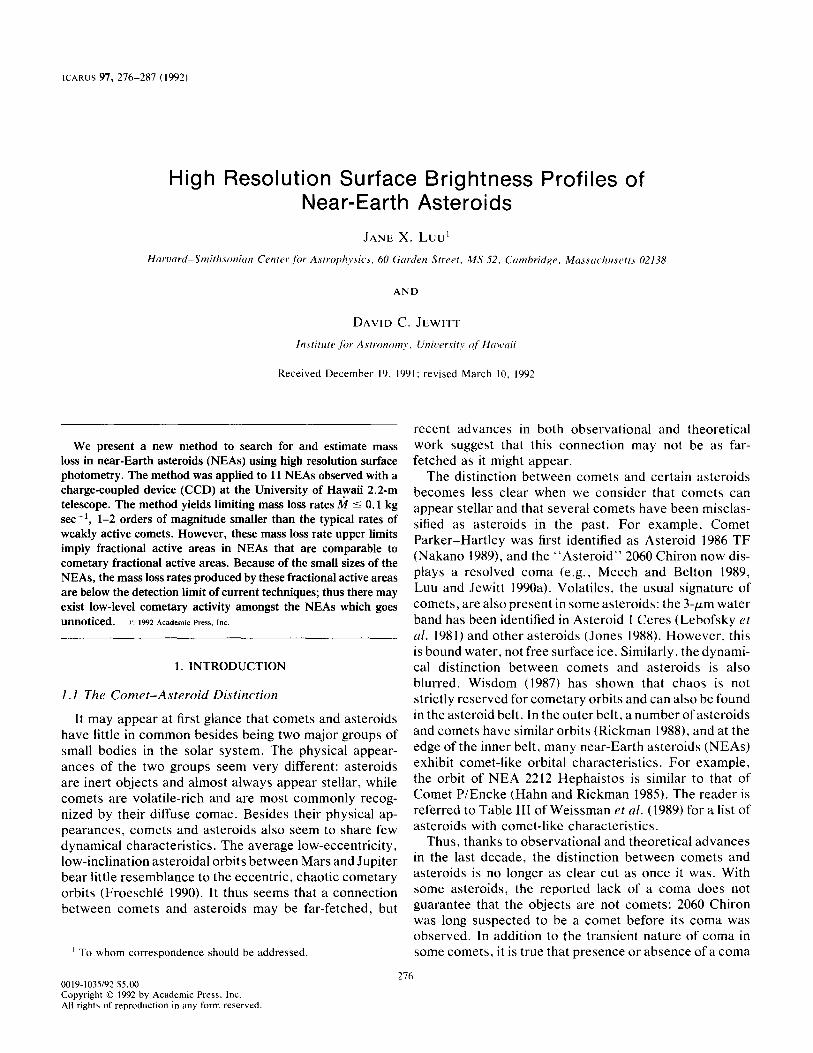
To obtain the asteroid profile, each image was rotated using a fifth order polynomial interpolation so that the asteroid trail was aligned parallel to the pixel rows on the CCD chip. Profiles of the NEAs and their reference stars were then obtained by averaging along the rows. Each star profile was averaged over the entire width of the star and each N EA profile averaged over the entire length of the NEA trail. Both profiles were then normalized and plotted on a single graph to search for any dissimilarities between the two profiles. Figure I shows log-linear pro- files of the 11 observed NEAs, superimposed upon the profiles of the reference stars. A few images show large scatter in the sky background (visible as large " sp ikes" or "d ips" ) , due to cosmetic imperfections in the CCD or low signal-to-noise. It is seen that most N EA profiles are very similar to their reference star profiles within the central 2" where most of the light is contained; there is no clear indication of comae, although there are some profiles with tantalizingly broad wings, such as in 1917 Cuyo, 3362 Khufu, and 1989 JA. In the cases of these NEAs, we examined carefully their profiles taken on other nights to verify the suggestion of coma. In no case did we find reproducible, unambiguously broadened profiles. We thus conclude that no coma was detected in any of the observed NEAs.

3. SURFACE BRIGHTNESS MODEL

We interpret the measured profiles using seeing- convolved images of model comets. We create images of model comets which possess the same image scale and PSF as the data, so that model profiles and real profiles can be compared directly. The steps involved in creating model profiles are (1) creation of a coma in an artificial image, (2) creation of a nucleus in the middle of the coma, and (3) convolut ion of the model images with the seeing. The details are as follows.

3.1. Simulation o f the Coma

In our models, it is assumed that the coma is spherically symmetric and in steady-state, i.e., the surface brightness of the coma is B(r) = K/r, where K is a constant of

P R O F I L E S O F N E A R - E A R T H A S T E R O I D S 279

101

~'~10 o .r.,

~ 1 0 -I

i 10-2

10-3

' " 1 ' ' " 1 . . . . I . . . . I . . . . I " " 1 . . . . I ' " • NEA1917

- - o- - Reference Star

1 2 3 4 5 6 7 Angular Dimnce [arcs~l

101

~ 10 0

0

~ 10.1

10.2

10-3

. . . . I . . . . I . . . . I . . . . I ' ' " 1 . . . . I' ' 1 " " • NEA 2059

- - o-- Reference Star

t ~ , r l , ~ , , l , , , , l ~ I I I I 1 1 1 1 1 1 1 1 1 i I J L I . L ~

I 2 3 4 5 6 7 Angular Distance [arcsec]

10 i

~ lO o m ~ 10-1

i 10-2

10"3

' " 1 . . . . I ' " ' 1 . . . . I " " l ' ' " l " " l ' " • NEA 2122

- o- - Reference Star

, , , I , , , 7 1 . . . . l ~ , t ] l , , , J l . . . . I , , l , , , ~

1 2 3 4 5 6 7 Angular Distance [arcsee]

0

m

z

10 ]

lO 0

10"1

10-2

10-3

' " 1 " I . . . . 1 ' " ' 1 . . . . I . . . . [ ' 1 " • NEA 2744

- - o- - Reference Star

- , ~ 1 , , , , J , , , , I , ~ ] , I t , , , J, , , , I , , t , I , , ' ~ 0 1 2 3 4 5 6 7 8

Angular Distance [aresec]

F IG. 1. The logar i thm of the surface br ightness is plot ted ve r sus linear d is tance in the plane of the sky (in a rcsec) for 11 N E A s and their re fe rence stars . The surface br igh tness is normal ized to unity at the peak of each profile.

proportionali ty and r is the impact parameter measured from the nucleus in the plane of the sky. The model images are 100 × 100 pixels in size, with the point-source nucleus located at the central pixel [pixel (50, 50)]. Each pixel subtends 0.2" × 0.2", as in the data. From the l/r surface brightness dependence, the intensity I of each pixel in the coma is determined by the integral

~ d x d y , (1)

where xj , x z are the left and right edges of a pixel, respec- tively, and y, and Yz are the lower and upper edges, respec- tively. Equation (1) has the solution

fyi2 (x2 K - dxdy

= K{y2 In(x2 + X~x22 + y~) + x2 ln(y2 + ~ x 2 + y2)

- Yz In(x] + X/~x21 + y2) _ xl ln(y 2 + X/~x2 + y2)

- Yl ln(x2 + X/~x22 + y2) _ x2 ln(y 1 + V~xz2 + y~)

+ Yl In(x1 + Xf~x21 + Y~) + xl ln(yl + X/x 2 + y~)}. (2)

Using Eq. (2), each coma pixel was assigned the proper intensity. This procedure was carried out identically for every model image.

3.2. Simulation of the Nucleus

Successive preconvolut ion models were distinguished from one another by the parameter "0, defined as the ratio of the coma cross-section Cc to the nucleus cross-sect ion Cn:

Cc Ic rt - Cn I , ' "0 -> 0. (3)

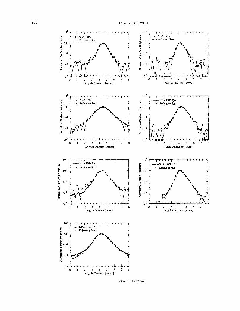
I¢ is the flux density scat tered by the coma, and I n is the flux density scattered by the nucleus. Ic is determined from aperture photometry on the model coma. The param- eter-0 can take on the values rt >- 0, with r / = 0 correspond- ing to a bare nucleus. The reference photomet ry aperture radius used is 1 arcsec. As can be seen in Fig. 2, this aperture is sufficiently large to take in most (86%) of the light in our N EA images, given the -< 1 arcsec seeing.

2 8 0 L U U A N D J E W I T T

10 ~

io ° . r - e ~

~ 10 d

~ 10 -2

z

10 -3 , 0

' ' " " " 1 . . . . I . . . . t . . . . t . . . . I . . . . ) . . . .

NEA 3200 - e- - Reference Star

', ~ ~"

~ ' ,

1

2 3 4 5 6 7 Angular Distance [arcsec]

101

. ~ 1 o °

10 q

~ 10 -2 z

10-3

. . . . . 1 ' " ' t . . . . I . . . . I . . . . 1 ' ' " 1 . . . . I ' " • NEA 3362

L _ c~ - Reference Star

1 2 3 4 5 6 7 8 Angular Distance [arcsec]

10 l

loo

10-1

i l0 2

10-3 0

, , i . . . . i . . . . i . . . . I . . . . I . . . . I ' ' 1 " ~ • NEA 3753

- ~ - Reference Star

o o @

6 ~ t J I . . . . I . . . . I . . . . I . . . . I . . . . I . . . . I , , 1 2 3 4 5 6 7

AngularDistance [arcsec]

t01

,.I

10 o .r.

~ 10 -1

10 2

z

10 .3

! , , , , i , , , , 1 , , , , i , , , , i , , , , 1 ~ , ~ , 1 , , , , i , , , • N E A 1 9 8 7 Q A

- c- - Reference Star

. . . . , . . . . , . . . .

1 2 3 4 5 6 7 Angular Distance [arcsec]

10 ]

.~ I0 o i~ t~ o

10.1

o 102

z

10 .3

, , , i . . . . i . . . . i . . . . I . . . . I . . . . I . . . . I '

• NEA 1989JA - o- - Reference Star

9 , : O

i b o q :

:, o i , ~ , , . ~ . . . . , . . . . ~ . . . . , . . . . ~ . . . . ) . . . . ~ , ,+.

0 1 2 3 4 5 6 7 Angular Distance [arcsec]

101

.~ I0 °

10.1

10_2

10 .3 0

• NEA 1989OB - - ~ - Reference Star

1 2 3 4 5 6 7 Ang~arDis tance [arcsec]

10 t

10 o "t~

~ 1 0 - 1 o'1

! ~o 102 z

10 .3

' ' " l . . . . I ' ' " l . . . . I ' " ' t . . . . I . . . . I ' ~ ' • NEA 1989PB

i

0 1 2 3 4 5 6 7 Angular Distance [arcsec]

F I G . 1 - - C o n t i n u e d

P ROF IL ES OF N E A R - E A R T H ASTEROIDS 281

1.1 1.0 0 .9

~, 0.8 0.7

~ 0 .6 0 .5

N 0 .4 0.3

~ 0 .2 0.1 0 .0

; ~ , , i , , , , i , , , , i , , , , i , , , , i , , , , i , , , f

0 .0 0 .5 1.0 1.5 2 .0 2.5 3 .0 Radius [arcsec]

3.5

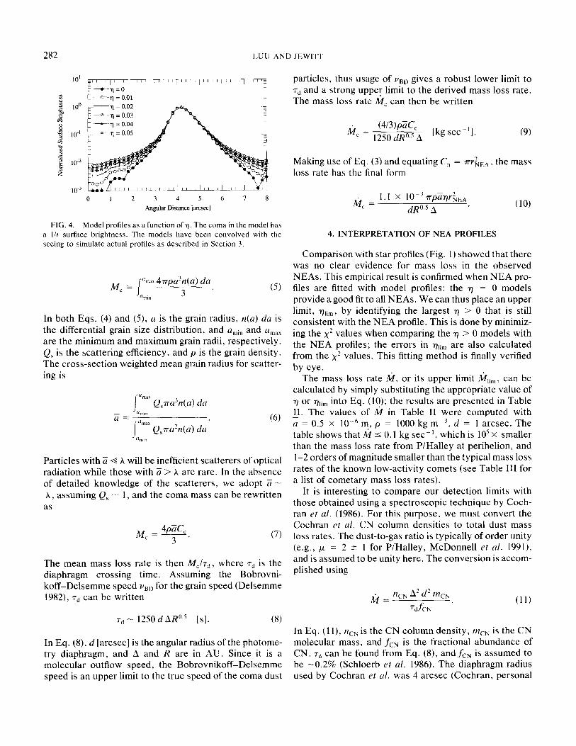
section. This is illustrated by Fig. 4, where a series of models separated by A-0 = 0.01 are shown. The models in Fig. 4 have been convolved with the typical Mauna Kea seeing to simulate profiles from actual images. The figure shows that, as r/increases, the profile is broadened, re- flecting the increasing fraction of coma. The model pro- files in the figure are clearly distinguishable, providing evidence for our resolution of m'o = 0.01.

3.4. Interpretation of the Model Profiles

The mass loss rate can be expressed as a function of the parameter '7. The total scattering cross-section of coma grains C~ within an aperture of radius d is

FIG. 2. The normal ized cumulat ive flux of a field star as a funct ion of radial dis tance. In this example , 86% of the light falls within a l -arcsec radius. f amax

Cc = QQra2n(a) da, (4) amin

3.3. Convolution of Model Images

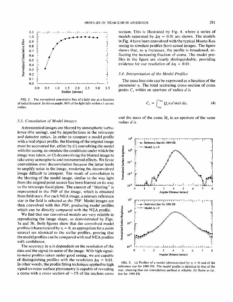
Astronomical images are blurred by atmospheric turbu- lence (the seeing), and by imperfections in the telescope and detector optics. In order to compare a model profile 101 with a real object profile, the blurring of the original image must be accounted for, either by (1) convolving the model m with the seeing, to simulate the conditions under which the ~. 100 image was taken, or (2) deconvolving the blurred image to ,~= take away atmospheric and instrumental effects. We favor ~ 10_ ~ convolution over deconvolution because the latter tends to amplify noise in the image, rendering the deconvolved image difficult to interpret. The result of convolution is "~ 10 .2 the blurring of the model image, similar to the way light z from the original point source has been blurred on its way to the telescope focal plane. The amount of "blurring" is l°S represented in the PSF of the image, which is obtained from field stars. For each NEA image, a primary reference

101 star in the field is selected as the PSF. Model images are then convolved with this PSF, producing model profiles m which can be directly compared with the NEA profile. ~ 100

We find that our convolved models are very reliable in ~ reproducing the image shape, as demonstrated by Figs. 3a and 3b. Both figures show that the convolved model ~ 101 profiles (characterized by ~ = 0, as appropriate for a point .~ source) are identical to the stellar profiles, proving that =-a 10 -2 the model profiles can be compared with real NEA profiles z ~ with confidence.

The accuracy in "0 is dependent on the resolution of the 10 -3

data and the signal-to-noise of the image. With high signal- to-noise profiles taken under good seeing, we are capable of distinguishing profiles with the resolution Art = 0.01. In other words, the profile fitting technique applied to high signal-to-noise surface photometry is capable of revealing a coma with a cross section of - 1 % of the nucleus cross

and the mass of the coma Mr in an aperture of the same radius d is

- • Reference Star for 1989 OB - --"°-- M~lel, ~1 = 0

6 ~ 6 ~ A 1 2 3 4 5 6 7

Angular Distance [arcsec]

'''l''''l''''l''''l''''I''''l''''['' + R e f e r e n c e Star for 1989 PB ---°--Model, ~1 = 0

1 2 3 4 5 6 7 Angular Distance [arcsec]

FIG. 3. (a) Profiles o f a model (character ized by ~ = 0) and of the reference star for 1989 OB. The model profile is identical to that of the star, showing that our convolut ion me thod is reliable. (b) Same as (a), but for 1989 PB.

282 LUU AND JEWITT

101

=o.o ~.~ 10 0 ~ ' ~q=0.02 ~ "~

=0.03 Y \ ~----*-- r I =0.04 / %

10.1

! ~ 10_2 Z

10-3 i t ~ l t J t l l , ~

0 1 2 3 4 5 6 7 8 Angular Distance [arcsec]

FIG. 4. Model profiles as a funct ion of'0. The coma in the model has a l / r surface br ightness . The models have been convolved with the seeing to s imulate actual profiles as described in Section 3.

Mc = f %'~ 4¢rpa3n(a) da amin 3 '

In both Eqs. (4) and (5), a is the grain radius, n(a) da is the differential grain size distribution, and ami n and am~ are the minimum and maximum grain radii, respectively. Qs is the scattering efficiency, and p is the grain density. The cross-sect ion weighted mean grain radius for scatter- ing is

f amax Qjra3n(a) da lmin

fj m,~ Q~Tra2n(a) da mm

Particles with ~ ~ X will be inefficient scatterers of optical radiation while those with ~ > ~ are rare. In the absence of detailed knowledge of the scatterers, we adopt ~ X, assuming Qs ~ 1, and the coma mass can be rewritten

a s

M~ - 4paCe 3

The mean mass loss rate is then Mc/r d, where ~-j is the diaphragm crossing time. Assuming the Bobrovni- kof f -Delsemme speed UBD for the grain speed (Delsemme 1982), r d can be written

~'d- 1250 d AR °5 [s]. (8)

In Eq. (8), d [arcsec] is the angular radius of the photome- try diaphragm, and A and R are in AU. Since it is a molecular outflow speed, the Bobrovnikoff -Delsemme speed is an upper limit to the true speed of the coma dust

particles, thus usage of uBD gives a robust lower limit to rd and a strong upper limit to the derived mass loss rate. The mass loss rate M~ can then be written

(4/3)p-dCc M~ - 1250dRO.S A [ k g s e c - q . (9)

Making use of Eq. (3) and equating C, = ~rNE A , the mass loss rate has the final form

/~/c = I.I x 10 3~pa'0ryE A (10) dR °5 A

4. INTERPRETATION OF NEA PROFILES

Comparison with star profiles (Fig. l) showed that there was no clear evidence for mass loss in the observed NEAs. This empirical result is confirmed when NEA pro-

(5) files are fitted with model profiles: the "9 = 0 models provide a good fit to all NEAs. We can thus place an upper limit, ~;~im, by identifying the largest ~ > 0 that is still consistent with the N EA profile. This is done by minimiz- ing the X 2 values when comparing the ~ > 0 models with the N EA profiles; the errors in ~lim are also calculated from the X 2 values. This fitting method is finally verified by eye.

The mass loss rate ~/, or its upper limit ~/lim, can be calculated by simply substituting the appropriate value of ,~ or T/lira into Eq. (10); the results are presented in Table II. The values of M in Table II were computed with (6) - a = 0 . 5 × 10 --6 m , p = 1000 kg m 3, d = 1 arcsec. The table shows that M -< 0.1 kg sec - j , which is 105 x smaller than the mass loss rate from P/Hal ley at perihelion, and 1-2 orders of magnitude smaller than the typical mass loss rates of the known low-activity comets (see Table II! for a list of cometary mass loss rates).

It is interesting to compare our detect ion limits with those obtained using a spectroscopic technique by Coch- ran et al. (1986). For this purpose, we must convert the Cochran et al. CN column densities to total dust mass

(7) loss rates. The dust-to-gas ratio is typically of order unity (e.g., /z = 2 +- 1 for P/Halley, McDonnell et al. 1991), and is assumed to be unity here. The conversion is accom- plished using

/~/ = nON A2 d2 m e N (1 1) "/'dEc N

In Eq. (11), ncNiS the CN column density, mCN is the CN molecular mass, and fCN is the fractional abundance of CN. ~'d can be found from Eq. (8), andfcN is assumed to be - 0 . 2 % (Schloerb et al. 1986). The diaphragm radius used by Cochran et al. was 4 arcsec (Cochran, personal

PROFILES OF NEAR-EARTH ASTEROIDS 283

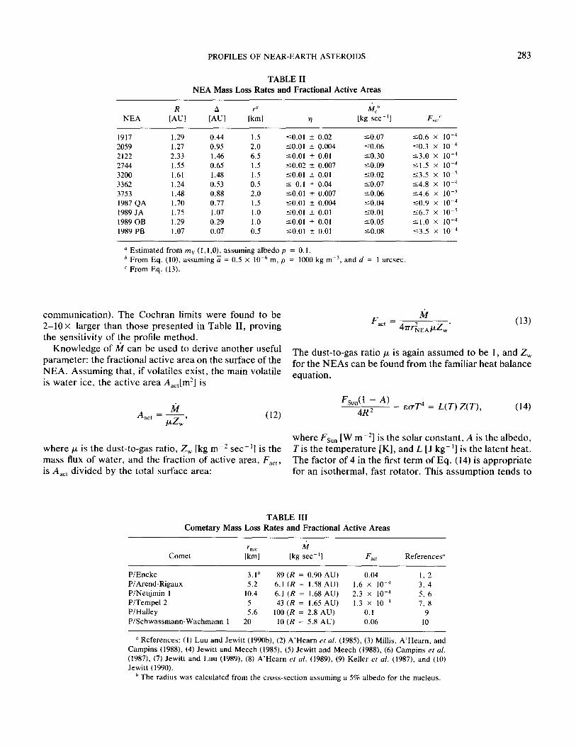
T A B L E II N E A Mass Loss Rates and Frac t iona l Active Areas

R A r a Mcb NEA [AU] [AU] [km] ,/ [kg sec-1] Fact c

1917 1.29 0.44 1.5 -<0.01 ± 0.02 -<0.07 -<0.6 x 10 -4 2059 1.27 0.95 2.0 -<0.01 -+ 0.004 -<0.06 -<0.3 × 10 -4 2122 2.33 1.46 6.5 -<0.01 -+ 0.01 -<0.30 -<3.0 x 10 -4 2744 1.55 0.65 1.5 -<0.02 + 0.007 -<0.09 -<1.5 x 10 -4 3200 1.61 1.48 1.5 -<0.01 -+ 0.01 -<0.02 -<3.5 x 10 -5 3362 1.24 0.53 0.5 -< 0.1 _+ 0.04 -<0.07 -<4.8 × 10 -4 3753 1.48 0.88 2.0 -<0.01 ± 0.007 -<0.06 -<4.6 × 10 -5 1987 QA 1.70 0.77 1.5 -<0.01 -+ 0.004 -<0.04 -<0.9 × 10 -4 1989 JA 1.75 1.07 1.0 -<0.01 ± 0.01 -<0.01 -<6.7 x 10 -5 1989 OB 1.29 0.29 1.0 -<0.01 ± 0.01 -<0.05 -<1.0 × 10 -4 1989 PB 1.07 0.07 0.5 -<0.01 -+ 0.01 -<0.08 -<3.5 x 10 4

Estimated from mv (1,1,0), assuming albedo p b From Eq. (10), assuming S = 0.5 x 10 -6 m, 0 c From Eq. (13).

= 0 . 1 . = 1000 kg m -3, and d = 1 arcsec.

communication). The Cochran limits were found to be 2-10x larger than those presented in Table II, proving the sensitivity of the profile method.

Knowledge of 3)/can be used to derive another useful parameter: the fractional active area on the surface of the NEA. Assuming that, if volatiles exist, the main volatile is water ice, the active area Aact[m 2] is

Aact = (12) /zZw'

where/z is the dust-to-gas ratio, Z w [kg m -2 sec -1] is the mass flux of water, and the fraction of active area, Fact, is Aac t divided by the total surface area:

Fac t - 47r r2EA/ZZ w. (13)

The dust-to-gas ratio/x is again assumed to be 1, and Zw for the NEAs can be found from the familiar heat balance equation,

Fsun(1 - A) 4R 2 eorT 4 = L ( T ) Z ( T ) , (14)

where Fsu, [W m-2] is the solar constant, A is the albedo, Tis the temperature [K], and L [J kg-1] is the latent heat. The factor of 4 in the first term of Eq. (14) is appropriate for an isothermal, fast rotator. This assumption tends to

T A B L E I I I C o m e t a r y Mass Loss Rates and Frac t iona l Active Areas

rnuc /~/ Comet [kml [kg sec-l] F a c t References"

P/Encke 3.1 t' 89 (R = 0.90 AU) 0.04 1, 2 P/Arend-Rigaux 5.2 6.1 (R = 1.58 AU) 1.6 x 10 4 3, 4 P/Neujmin 1 10.4 6.1 (R = 1.68 AU) 2.3 x 10 -4 5, 6 P/Tempel 2 5 43 (R = 1.65 AU) 1.3 x 10 3 7, 8 P/Halley 5.6 100 (R = 2.8 AU) 0.1 9 P/Schwassmann-Wachmann 1 20 10 (R = 5.8 AU) 0.06 10

References: (1) Luu and Jewitt (1990b), (2) A 'Hearn et al. (1985), (3) Millis, A 'Hearn , and Campins (1988), (4) Jewitt and Meech (1985), (5) Jewitt and Meech (1988), (6) Campins et al. (1987), (7) Jewitt and Luu (1989), (8) A 'Hearn et al. (1989), (9) Keller et al. (1987), and (10) Jewitt (1990).

b The radius was calculated from the cross-section assuming a 5% albedo for the nucleus.

284 LUU AND JEWITT

' I I I I I I I I ] I I • N E A s ' l

o Other Comets 3 - *- - Comet Halley

2

Neujmin 1 oo Arend-Rigaux 1 SW1

0

- 2 - -

-3 : 1 1 I I J ~ l I I ] I I I I I I I I J ] I I I I [ I-I I 0 l 2 3 4 5 6

R [ A U ]

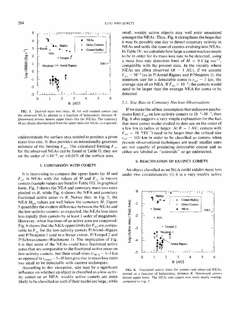
FIG. 5. Derived mass loss rates, /V/. for well studied comets and the observed NEAs plotted as a function of heliocentric distance R. Downward arrows denote upper limits (for the NEAs). The cometary M are clearly distinguished from the upper limits for NEAs, as expected.

"t o "&.. Halley

- Encke -._ _ o - , o - ~

IAA o Tempel 2

u n d e r e s t i m a t e the su r face a r e a n e e d e d to p r o d u c e a g iven mass loss ra te . It thus p r o v i d e s an in t en t iona l ly g e n e r o u s e s t i m a t e o f the l imi t ing F ~ t . The c a l c u l a t e d l imit ing F~t for the o b s e r v e d N E A s can be found in T a b l e I I ; t hey are on the o r d e r o f - < 1 0 4 o r -<0.01% of the su r face area .

5. COMPARISON WITH COMETS

It is i n t e r e s t i ng to c o m p a r e the u p p e r l imits for ~ / a n d F~ct in N E A s wi th the va lue s o f M and F~t in k n o w n c o m e t s ( s a m p l e va lue s a re l i s t ed in Tab le III) . In g raph ica l fo rm, Fig . 5 s h o w s the N E A and c o m e t a r y mass loss ra tes p l o t t ed vs R, whi le Fig. 6 s h o w s the N E A and c o m e t a r y f r ac t i ona l a c t i ve a r e a s vs R. N o t i c e tha t , in Fig. 5, the N E A / ~ l i m va lues a re well b e l o w the c o m e t a r y M. F igure 5 quant i f i es the e v i d e n t d i f f e r ence b e t w e e n the N E A s and the l o w - a c t i v i t y c o m e t s : as e x p e c t e d , the N E A s lose m a s s less r a p i d l y then c o m e t s by at leas t 1 o r d e r of magn i tude . H o w e v e r , w h e n f r ac t ions o f an ac t ive a r e a a re c o m p a r e d , Fig . 6 s h o w s tha t the N E A u p p e r l imits for F~,~t a re c o m p a - rab le to F,c t for the l o w - a c t i v i t y c o m e t s P / A r e n d - R i g a u x and P / N e u j m i n 1 (and to a l e s se r ex t en t , P / T e m p e l 2 and P / S c h w a s s m a n n - W a c h m a n n 1). The imp l i ca t ion o f Fig. 6 is tha t s o m e o f the N E A s could have f rac t iona l ac t ive a r e a s tha t a re c o m p a r a b l e to the f r ac t iona l ac t ive a r eas on l o w - a c t i v i t y c o m e t s , bu t the i r smal l s izes (rNE A - - 1-3 km as o p p o s e d to r~om~ t ~ 5 - 1 0 kin) g ive r ise to mass loss ra tes t oo smal l to be d e t e c t a b l e wi th cu r r en t t e chn iques .

A c c o r d i n g to this v i ewpo in t , s ize m a y be a s ignif icant in f luence on w h e t h e r an ob j ec t is c lass i f ied as a l ow-ac t iv - i ty c o m e t o r an N E A : w e a k l y ac t ive c o m e t s a re m o r e l ike ly to be c lass i f ied as such if the i r nucle i a re large , while

smal l , w e a k l y ac t i ve o b j e c t s m a y wel l ex i s t u n n o t i c e d a m o n g s t the N E A s . Thus , Fig . 6 s t r e n g t h e n s the h o p e tha t it m a y be p o s s i b l e one d a y to d e t e c t c o m e t a r y a c t i v i t y in N E A s and se t t le the i s sue o f c o m e t s e v o l v i n g into N E A s . In Tab le IV, we ca l cu l a t e h o w large a c o m e t nuc l eus needs to be in o r d e r for its m a s s loss ra te to be d e t e c t e d , us ing a mass loss ra te d e t e c t i o n l imit o f ~ / = 0.1 kg sec J, c o m p a t i b l e wi th the p r e s e n t da ta . In the v ic in i ty w h e r e N E A s a re o f t en o b s e r v e d (R - 1 A U ) , if we a s s u m e F.~t ~ 10 4 (as in P / A r e n d - R i g a u x and P / N e u j m i n 1), the m i n i m u m size for a d e t e c t a b l e c o m a is rcrit ~ I km, the a v e r a g e s ize o f an N E A . I fFac t < 10 4, the c o m e t s w o u l d need to be la rger than the a v e r a g e N E A for c o m a to be d e t e c t e d .

5.1. Size Bias in Cometary Nucleus Observations

If we m a k e the ad hoc a s s u m p t i o n tha t u n k n o w n m e c h a - n i sms l imit F,ct on l o w - a c t i v i t y c o m e t s to 10 -4 -10 5, then Fig. 6 a lso sugges t s a ve ry s imple e x p l a n a t i o n for the fac t that mos t c o m e t nucle i s t ud i e d to d a t e a re on the o r d e r o f a few km in rad ius o r la rger . At R = I A U , c o m e t s wi th Fac t = 10 4 ( 1 0 5) need to be l a rge r t han the cr i t ica l size rcr~t - 1(3) k m in o r d e r to be c lass i f i ed as c o m e t s w h e n p r e se n t o b s e r v a t i o n a l t e c h n i q u e s a re u sed : sma l l e r ones are not c a p a b l e o f p r o d u c i n g d e t e c t a b l e c o m a e and so e i the r a re l a be l e d as " a s t e r o i d s " o r go u n d e t e c t e d .

6. REACTIVATION OF EXTINCT COMETS

A n ob j ec t c lass i f ied as an N E A cou ld exh ib i t m a s s loss unde r two c i r c u m s t a n c e s : (1) it is a v e r y w e a k l y ac t ive

-2

> -3 <

.~ -4

-5

' ~ ' ' l l ~ ' ' l l ~ ' ' l l ' ~ ' l l ' l ' l J b ~ .g Halley , ' [ * " "~I '~" ~ / - - * Comet Halley

/ o Other Comets o Encke U • NEAs SW1

o IAA

Tempel 2

~ $ Neujmin 1

~ U@~ ~ ' ~ Arend-Rigaux

~ 1 , , L , k , I t l L l ~ t ,~

0 l 2 3 4 5 R [ A U ]

I

6

FIG. 6. Fractional active areas for comets and observed NEAs, plotted as a function of heliocentric distance R. Downward arrows denote upper limits. The NEAs and comets now more nearly overlap, compared to Fig. 5.

P R O F I L E S O F N E A R - E A R T H A S T E R O I D S 285

TABLE IV Critical Radius for Detectable Mass Loss Rate

/'crit a rcrit a Fac t [km] Fact [k]

R = 1 A U R = 2 A U 10 -1 0 .03 10 - I 0.1 10 -2 0.1 10 2 0.3 10 -3 0.3 10 -3 1.0 10 -4 0 .9 10 4 3 .2 10 -5 3 .0 10 -5 10.1

" rcnt w a s c a l c u l a t e d a c c o r d i n g to E q . (10), a s s u m - ing a 5 % a l b e d o a n d a d e t e c t i o n l imit M = 0.1 k g s e e - i.

comet which has evolved into an NEA orbit, but its mass loss rate is too small to be easily detected (see previous section, Section 5. I); or (2) it is an " ex t i nc t " comet which has been reactivated. The first circumstance has not been proven to occur, although dynamical studies have not ruled it out (Weissman et al. 1989); likewise, the second circumstance has not been confirmed. Complete mantling of the nucleus may be impossible due to porosity, or due to cracks in the surface produced by thermal stresses (Kiihrt 1984). If we assume that comets evolve into NEAs by complete mantle coverage, it is an interesting exercise to estimate the likelihood of detecting a reactivated comet.

Two obvious possibilities present themselves as mecha- nisms of reactivation:

(I) individual impacts that destroy part of the mantle so as to expose the volatiles underneath;

(2) mantle erosion due to micrometeoroid bom- bardment.

Undoubtedly, other mechanisms exist that can also create openings in the mantle; however , we restrict our discus- sion to the two mechanisms mentioned above because these processes are sufficiently understood that the basic physical parameters are established, allowing us to assess their likelihood as reactivation mechanisms. We also as- sume that, regardless of the reactivation mechanism, the length of the active period (the time it takes for the mantle to regrow and recover the active area) is sufficiently long that the nucleus has a chance of being observed while outgassing. Various models have suggested that mantle growth requires a timescale on the order of one to a few orbital revolutions (e.g., Fanale and Salvail 1984, Grian et al. 1989, Rickman et al. 1990), corresponding to perhaps 10 years of outgassing activity, once initiated.

The efficiencies of the two mechanisms listed above are estimated in the Appendix. The results of the calculations can be summarized as follows:

1. Single- impact cratering. For a 1-kin radius NEA,

the collision time for an impact large enough to produce a detectable coma is - 3 x 1013 sec or 1 x 106 years. If it takes 1-2 N E A orbital revolutions ( - 1 0 years) for the mantle to cover the surface, then the chance of witnessing this reactivation event is 10/106 years, or 10 .5 . Therefore , we would need to examine 105 NEAs in order to observe one such e v e n t - - a daunting requirement , since the num- ber of known NEAs is ~105.

2. Microbombardment erosion. Assuming an erosion rate similar to that of the moon, we calculate that a 5-cm- thick mantle can be eroded away in - 5 × 107 years, or approximately an N EA lifetime. Given the long erosion time scale, it is unlikely that we will observe a comet reactivated by microbombardment erosion.

Based on our calculations, we conclude that detect ion of an impact-reactivated comet nucleus in an NEA orbit is not easily achieved, mostly because of the competi t ion between the timescale for surface mantle coverage (short) and the timescale for reactivation (long). However , the detection of a very weakly (but continuously) active comet may be more feasible. The low-activity comet P/ Encke is presently in an NEA-like orbit, suggesting that some low-activity comets can evolve dynamically into an NEA-iike orbit. Figure 6 suggests that o ther Encke-like objects may exist among NEAs.

7. FUTURE WORK

In this paper, we have described a profile-fitting method that is sensitive to mass loss rates >0.1 kg/sec, when applied to kilometer-sized NEAs. For comparison, this is 4 to 5 orders of magnitude smaller than the mass loss rate from P/Halley when near perihelion (see Fig. 5). Profile- sitting is thus competi t ive with other techniques used to search for mass loss in asteroids, including spectroscopic searches published to date. Unfortunately, NEAs pos- sessing fractional active areas similar to those of weakly active comets would fall at, or slightly beneath, the limits of detection of the existing methods. For example, the weakly active comets P/Arend-Rigaux and P/Neujmin 1 lose mass at about I0 kg/sec, but have surface areas about 100x larger than those of NEAs in our sample. Thus the present observations cannot be used to reject the hypothesis that some NEAs are outgassing from fractional active areas similar to those of weakly active comets .

Future profile measurements from Mauna Kea will ben- efit from several recent technical advances. First, new anti-reflection coated CCDs installed at the UH 2.2-m telescope have quantum efficiencies twice that of the GEC CCD used for the initial observations. Second, a new fast- response autoguider allows the telescope to be tracked with high accuracy at asteroidal rates, decreasing the area on the CCD from which the faint wings of the surface brightness profile must be recovered. Third, a new Casse-

286 LUU AND JEWITT

grain secondary has been built to remove residual aberra- tions present in the 2.2-m primary. The telescope has recently given images better than 0.3" FWHM, and the intensity in the wings of the images is significantly re- duced. Together, these improvements will allow us to increase the sensitivity of the profile-fitting method to weak coma by more than 1 order of magnitude.

8. C O N C L U S I O N S

F rom high resolution surface pho tomet ry of NEAs , we conclude that:

(1) There was no compell ing evidence for comae in the 11 obse rved N E A s (see Table II).

(2) The upper limits to allowed mass loss rates are of order

3;1 _< 0.1 kg sec ~,

which is 10-100 x smaller than the typical rates reported in weakly active comets .

(3) The present application of the profile-fitting tech- nique implies that we cannot exclude the existence of N E A s with fractional active areas comparable to the frac- tional act ive areas on low-activity comets . Thus, it is possible that some N E A s could be as active (per unit area) as are some comets , but the very small sizes of typical N E A s (radius ~ 1 - 3 km) may preclude their detection with current instrumentat ion.

(4) Likewise , low-activity comets need to be larger than ~ a few km in radius for their weak comae to be detected; smaller ones may go unnoticed or be classified as asteroids. This may in part explain the apparent under- abundance of comet nuclei with radii <1 km.

A P P E N D I X

Reactivation Mechanisms for Comet Nuclei l. Single-impact cratering. From impact craters on the surfaces of

the planets and their planetary satellites, we know that impact cratering by meteoroids is common . We wish to determine what kind of impact is capable of removing a large enough piece of the mantle for cometary activity to be detectable, and on what t imescale this takes place. Since the gravity of a 1-kin-radius nucleus is very small, any ejecta produced by impact cratering is likely to escape from the surface (the escape velocity v~ = 0.7 m sec 1). Based on the wealth of research on impact cratering, we can relate the kinetic energy of the projectile to the diame- ter of the resul tant crater (Gault 1973, Gault 1974);

D = 1.342 = 10 s pI~'p~°SKE°29(sin Ot r3,

where D is the d iameter of the crater (m), pp is the densi ty of the projectile (kg m 3), 0T is the densi ty of the target (kg m-3), KE is the kinetic energy of the projectile (J), and 0 is the incident angle measured from the target surface. This result was derived from hyperveloci ty impact exper iments on basalt , and is a s sumed to be roughly applicable for impact into a

comet mantle. F rom Table II, we calculate that the active area needs to be - a few x 103 m 2 for the coma to be detected by the profile method. It we a s sume normal incidence (0 = 90°), a projectile densi ty and a target densi ty pp - PT = 1000 kg m -~, an active area A - 3000 m 2 (D - 61.8 m), and a projectile velocity vp = 30 km/sec (as is appropriate for an object in orbit at R - I AU), this yields the projectile mass mp 8.8 × 10 z kg, i.e., a projectile radius ap - 0.6 m. The flux of particles with a ~ 0.6 m at R I AU is - 1 0 - - ' sec -t (Morrill et al. 1983). This implies that, for a 1-km-radius NEA, the impact ing particle flux received at the surface is 3 x 10 14 sec i Thus the collision t ime for an impact large enough to produce a detectable coma is - 3 x 10 t3 sec or 106 years. This t imescale is slightly smaller than the dynamical lifetime of an N E A (107-108 years), suggest ing that this event could only happen ~ 10 x in an N E A lifetime, and is thus unlikely to be the principal reactivation mechanism. Our result disagrees with that of Fe rnandez (1990), who es t imated that impact craters with d iameters on the order of 100 m can be produced every few revolut ions on 5-km-radius objects like P/Halley and P/Arend-Rigaux and are responsible for excavat ing the mantle .

2. Microbombardment erosion. Lunar rocks and regolith f ragments are covered by microcraters ( /xm-cm in size), providing ample evidence for the erosion of the surface by micrometeoroids . How long would it take micrometeoroids to erode the mant le? The mant le of Comet Halley is es t imated to be a few cm thick (e.g., lp and Rickman 1986). If, for definiteness, we a s sume a mantle th ickness of 0.05 m, and the lunar erosion rate - 10 ,~/year (Ashwor th 1978), the mant le can then be eroded away in 5 × 107 years (1-2 orders of magni tude less efficient than single impact cratering), or approximate ly an N E A lifetime.

A C K N O W L E D G M E N T S

This work was supported in part by a Smi thsonian Postdoctoral Fel- lowship to J. X. Luu and a grant f rom the National Science Foundat ion to D. C. Jewitt. We thank R. Millis and R. A. Brown for very valuable suggest ions.

R E F E R E N C E S

A'HEARN, M. F., P. V. BIRCH, P. D. FELDMAN, AND R. L. MILLIS 1985. Comet Encke: Gas product ion and l ightcurve. Icarus 64, 1-10.

A'HEARN, M. F., H. CAMPINS, D. G. SCHLEICHER, AND R. L. MILLIS 1989. The nucleus of P /Tempel 2. Astrophys. J. 347, 1155-1166.

ASHWORTH, D. G. 1978. Lunar and planetary impact erosion. In Cosmic Dust. (J. A. M. McDonnel l , Ed.), pp. 427-526. Wiley, Chichester .

CAMPINS, H., M. F. A'HEARN, AND L. A. MCFADDEN 1987. The bare nucleus of Comet P /Neujmin I. Astrophys. J. 316, 847-857.

COCHRAN, W. D., A. L. COCHRAN, AND E. S. BARKER 1986. Spectros- copy of asteroids in unusual orbits. In Asteroids', Comets, Meteors H (C.-I. Lagerkvist , B. A. Lindblad, H. Lunds ted t , and H. Rickman, Eds.), pp. 181-185. Uppsa la Univ. Press, Uppsala .

DEGEWIJ, J. 1980. Spect roscopy of faint as teroids , satellites, and com- ets. Astrophys. J. 85, 1403-1412.

DELSEMME, A. H. 1982. Chemical composi t ion of cometa ry nuclei. In Cmnets (L. L. Wilkening, Ed.), pp. 85-130. Univ. of Ar izona Press, Tucson.

DRUMMOND, J. D., AND E. K. HEGE 1989. Speckle interferometry of asteroids. In Asteroids H (R. P. Binzel, T. Gehrels , and M. S. Mat- thews, Eds.), pp. 171-191. Univ. of Ar izona Press, Tucson .

FANALE, F. P., AND J. R. SALVAIL 1984. An idealized short-period comet model: Surface insolation, HzO flux, dus t flux, and mantle evolution. Icarus 60, 476-51 I.

FERNANDEZ, J. 1990. Collisions of comets with meteoroids . In Aster- oids, Cmnets, and Meteors HI (C.-I. Lagerkvis t , H. Rickman, B. A.

PROFILES OF NEAR-EARTH ASTEROIDS 287

Lindblad, and M. Lindgren, Eds.), pp. 309-312. Uppsala Univ. Press, Uppsala.

FROESCHL~, C. 1990. Chaotic behavior of asteroidal and cometary or- bits. In Asteroids, Comets, and Meteors 111 (C.-I. Lagerkvist, H. Rickman, B. A. Lindblad, and M. Lindgren, Eds.), pp. 63-76. Uppsala University Press, Uppsala.

GAULT, D. E. 1973. Displaced mass, depth, diameter, and effects of oblique trajectories for impact craters formed in dense crystalline rocks. Moon 6, 32-44.

GAULT, D. E. 1974. Impact Cratering. In A Primer in Lunar Geology (R. Greeley and P. Schultz, Eds.), pp. 137-175. NASA Tech Memo- randum TM X-62, 359.

GAULT, D. E,, F. HORZ, AND J. B. HARTUNG 1972. Effects of microcra- teEing on the lunar surface. Proc. Third Lunar Sci. Conf., Vol. 3, pp. 2713-2734.

GRI]N, E., J. BENKHOFF, H. FECHTIG, P. HESSELBARTH, J. KLINGER, H. KOCHAN, H. KOHL, D. KRANKOWSKY, P. L.~MMERZAHL, W. SE- BOLDT, T. SPOHN, AND K. THIEL 1989. Mechanisms of dust emission from the surface of a cometary nucleus. Adv. Space Res. 9, 133-137.

HAHN, G., AND H. RICKMAN 1985. Asteroids in cometary orbits. Icarus 61, 417-442.

HARTMANN, W. K., O. J. THOLEN, K. MEECH, AND D. P. CRUIKSHANK 1990. 2060 Chiton: Colorimetry and cometary behavior. Icarus 83, 1-15.

Ia, W. H., AND H. RICKMAN 1986. A comparison of nucleus surface models to space observations of Comet Halley. In Proceedings o f the Comet Nucleus Sample Return Mission Workshop, ESA SP-249.

JEWlTT, D. C. 1990. The persistent coma of Comet P/Schwassmann- Wachmann 1. Astrophys. J. 351, 277-286.

JEWITT, D. C., AND J. X. L uu 1989. A CCD portrait of Comet P/Tempel 2. Astrophys. J. 97, 1766-1790.

JEWITT, D. C., AND K. MEECH 1985. Rotation of the nucleus of P/ Arend-Rigaux. Icarus 64, 329-335.

JEWITT, D. C., AND K. MEECH 1988. Optical properties of cometary nuclei and a preliminary comparison with asteroids. Astrophys. J. 328, 974-986.

JONES, T. D. 1988. An Infrared Reflectance Study o f Water in Outer Belt Asteroids: Clues to Composition and Origin. Ph.D. Thesis, Univ. of Arizona.

KELLER, H. U., W. A. DELAMERE, W. F. HUEBNER, H. J. RE1TSEMA, H. U. SCHMIDT, F. L. WHIPPLE, K. WILHELM, W. CURDT, R. KRAMM, N. THOMAS, C. ARPIGNY, C. BARBIERI, R. M. BONNET, S.

CAZES, M. CORADINI, C. B. COSMOVICI, D. W. HUGHES, C. JAMAR, D. MALAISE, K. SCHMIDT, W. K. H. SCHMIDT, AND P. SEIGE 1987. Astron. Astrophys. 187, 807.

KOHRT, E. 1984. Temperature profiles and thermal stresses in cometary nuclei. Icarus 60, 512-521.

LEBOFSKY, L. A., M. A. FEIERBERG, A. T. TOKUNAGA, H. P. LARSON, AND J. R. JOHNSON 1981. The 1.7- to 4.2-/zm spectrum of Asteroid 1 Ceres: Evidence for structural water in clay minerals. Icarus 48, 453-459.

Luu, J. X., AND D. C. JEWITT 1990a. Cometary activity in 2060 Chiron. Astrophys. J. 100, 913-932.

Luu , J. X., AND D. C. JEWITT 1990b. The nucleus of Comet P/Encke. Icarus 86, 69-81.

McDoNNELL, J. A. M., P. L. LAMY, AND G. S. PANKIEWICZ 1991. Physical properties of cometary dust. In Comets in the Post-Halley Era (R. L. Newburn, Jr., M. Neugebauer, and J. Rahe, Eds.), Vol. 2, pp. 1043-1073. Kluwer, Dordrecht.

MEECH, K., AND M. BELTON 1990. 1AU Circular 4770. MORFILL, G. E., H. FECHTIG, E. GRON, AND C. K. GOERTZ 1983.

Some consequences of meteoroid impact on Saturn's rings. Icarus 55, 439-47.

NAKANO, S. 1989. IAU Circular 4752. RICKMAN, H. 1988. Relations between small bodies: Discussion. Celes-

tial Mechanics 43, 413-416. RICKMAN, H., B. ,~. S. GUSTAFSON, AND J. A. FERNANDEZ 1990. Model

calculations of mantle formation on comet nuclei. In Asteroids, Com- ets, and Meteors 111 (C.-I. Lagerkvist, H. Rickman, B. A. Lind- blad, and M. Lindgren, Eds.), pp. 423-426. Uppsala Univ. Press, Uppsala.

SCHLOERB, F. P., W. M. KINZEL, D. A. SWADE, AND W. M. IRVINE 1986. HCN production from Comet Halley. In 20th ESLAB Sympo- sium on the Exploration o f Halley's Comet (B. Battrick, E. J. Rolfe, R. Reinhard, Eds.), pp. 577-581. ESA Publ. Div., ESTEC, Noordwijk.

SPINRAD, H., J. STAUFFER, AND R. L. NEWBORN 1979. Optical spectro- photometry of Comet Tempel 2 far from the Sun. Publ. Astron. Soc. Pac. 92, 707-711.

WEISSMAN, P. R., M. F., A'HEARN, L. A. McFADDEN, AND H. RICK- MAN 1989. Evolution of comets into asteroids. In Asteroids H (R. P. Binzel, T. Gehrels, and M. S. Matthews, Eds.), pp. 880-920. Univ. of Arizona Press, Tucson.

WISDOM, J. 1987. Chaotic dynamics in the Solar System. Icarus 72, 241-275.