high resolution stochastic downscaling method for ocean

1

High resolution stochastic downscaling method for ocean forecasting models and its application to the Red Sea dynamics

Georgy I. Shapiro1, Jose M. Gonzalez-Ondina2, Vladimir N. Belokopytov3

1School of Biological and Marine Sciences, University of Plymouth, Plymouth, PL4 8AA, UK 2University of Plymouth Enterprise LTD, Plymouth, PL4 8AA, UK 5 3Marine Hydrophysical Institute, Russian Academy of Sciences, Sevastopol, 299011, Russia

Correspondence to: Georgy I. Shapiro ([email protected])

https://doi.org/10.5194/os-2020-119Preprint. Discussion started: 11 January 2021c© Author(s) 2021. CC BY 4.0 License.

2

Abstract. High-resolution modelling of a large ocean domain requires significant computational resources. The main

purpose of this study is to develop an efficient tool for downscaling the lower resolution data such as available from 10

Copernicus Marine Environment Monitoring Service (CMEMS). Common methods of downscaling CMEMS ocean models

utilize their lower resolution output as boundary conditions for local, higher resolution hydrodynamic ocean models. Such

methods reveal greater details of spatial distribution of ocean variables; however, they increase the cost of computations, and

often reduce the model skill due to the so called ‘double penalty’ effect. This effect is a common problem for many high-

resolution models where predicted features are displaced in space or time. This paper presents a Stochastic Deterministic 15

Downscaling (SDD) method, which is an efficient tool for downscaling of ocean models based on the combination of

deterministic and stochastic approaches. The ability of the SDD method is first demonstrated in an idealised case when the

true solution is known a priori. Then the method is applied to create an operational eddy-resolving Stochastic Model of the

Red Sea (SMORS) with the parent model being the eddy-permitting Mercator Global Ocean Analysis and Forecast System.

The stochastic component is data-driven rather than equation-driven and applied to the areas smaller than the Rossby radius, 20

where distributions of ocean variables are more coherent. The method, based on objective analysis, is similar to what is used

for data assimilation in ocean models, and stems from the philosophy of 2D turbulence. The SMORS model produces higher

resolution (1/24th degree latitude mesh) oceanographic data using the output from a coarser resolution (1/12th degree mesh)

parent model available from CMEMS. The values on the high-resolution mesh are computed under condition of

minimisation of the cost function which represents the error between the model and true solution. The SMORS model has 25

been validated against Sea Surface Temperature and ARGO floats observations. Comparisons show that the model and

observations are in good agreement and SMORS is not subject to the ‘double penalty’ effect. SMORS is very fast to run on a

typical desktop PC and can be relocated to another area of the ocean.

30

1 Introduction

A deterministic approach in ocean modelling based on solving differential equations is capable of producing high quality

forecasts/hindcasts, both for research and operational needs and is currently a mainstream in numerical modelling of the ocean.

Ocean models have matured through multiple improvements including better numerical schemes, spatial discretization,

parameterizations, and data assimilation. Modern ocean models do not solve the full Navier-Stokes or Reynolds equations, 35

instead they tend to make the traditional and hydrostatic Boussinesq approximations and various parameterisations of

unresolved processes (Miller, 2007; Fox-Kemper et al., 2019; Lindsay, 2017; Ezer and Mellor, 2004; Bruciaferri et al, 2019).

However, the enhancement of model resolution using such approach involves a significant increase in the computational cost.

For example, doubling the horizontal resolution in both directions requires approximately ten times more calculations, taking

into account the necessity of reducing the time step and increasing the overhead due to data exchange between the nodes of a 40


3

High Performance Computer. There is also an increased conceptual difficulty to resolve deterministically very small-scale

processes due to the turbulent and chaotic nature of motion at a small scale.

In contrast to early ocean models which were applied to highly idealized cases and did not require any observational data, e.g.

(Bryan, 1963), modern models use real-world data in addition to the universal laws of physics. The data are used for model

initialisation, tuning the numerical parameters such as diffusion/viscosity coefficients, validation and data assimilation. Data 45

assimilation improves the description of ocean state used as the initial condition for the forecasting step. There are many

different forms of data assimilation. One of the most efficient methods is optimal interpolation (OI) (Gandin 1959; Gandin

1965; Fletcher, 2017) which uses statistical properties of real-world data rather than equations of motion or prescribed spatial

dependences]. The philosophy of combining deterministic and stochastic (random) behaviour of fluids has a long history. For

example the Reynolds equations and their modern versions used in ocean modelling, based on simple decomposition of an 50

actual instantaneous quantity into time-averaged and fluctuating quantities and taking the averages of non-linear terms, see

e.g. (Tennekes and Lumley, 1992). More advanced methods of describing the chaotic movements at smaller scale have been

developed in the statistical theory of turbulence, see e.g. (Kolmogorov, 1941; Monin and Yaglom,1971; Frisch, 1995). The

OI method further extends ideas originated in the theory of statistical turbulence and was the method of choice for operational

numerical weather prediction centres in the 1980s and early 1990s. 55

The basis of OI is the minimisation of a cost function which represents a measure of the difference between the estimated and

true values. The OI considers the data fields as realisations of random processes and it studies the statistical links represented

by either structure functions or covariances between data points in a way similar to the theory of fully developed turbulence

(Gandin and Kagan, 1976). An important feature of the method is that, in order to calculate the interpolating coefficients, it

only requires the knowledge of statistical moments of the second order and does not use any a priori hypothesis about the 60

dependence of the weights on the distance from the interpolation points as it is used in alternative methods of objective analysis

(Cressman 1959, Vasquez, 2003). In those alternative methods the weighting coefficients are calculated as a prescribed

analytical function of distance, and hence do not require the knowledge of the statistical properties of the actual field of interest.

In this paper we have tested a hypothesis that a similar technique, hereafter called Stochastic-Deterministic Downscaling, or

SDD, based on the statistical properties of ocean parameters such as temperature, salinity and velocity, can be used to achieve 65

a higher resolution in ocean modelling by downscaling the results of a parent deterministic model. Basically, the data are

treated as having two components, a low resolution, slowly varying component which is computed using deterministic

equations, and a high resolution fast varying component where the data are treated as random processes. As in the theory of

turbulence, the statistical properties of the smaller scale processes are often much more stable than the data themselves, see

e.g. (Monin and Yaglom,1971; Tennekes and Lumley, 1992). 70

The assimilation of observational data is widely used in operational ocean modelling, see e.g. (Dobricic et al, 2007; Dobricic

and Pinardi, 2008; Korotaev et al, 2011; Mirouze et al, 2016) . However, the application of a similar approach for high-

resolution model downscaling should be considered as experimental at this stage. This is why the SDD method is first tested

and assessed by application to an idealised case of a region filled with multiple mesoscale eddies where the true solution is


4

known. While the proposed SDD method has a generic nature, the focus of this paper is on its application to the Red Sea, 75

which has complicated coastline and multiple islands. The main section of the paper describes the development and properties

of operational eddy-resolving Stochastic Model for the Red Sea (SMORS) at 1/24th degree resolution based on a parent eddy-

permitting model at 1/12th degree resolution, which outputs are accessible via Copernicus Marine Environment Monitoring

Service (CMEMS, 2020).

2 Materials and methods 80

2.1 The algorithm

The Stochastic-Deterministic Downscaling (SDD) uses the methodology developed for the original version of the Optimal

Interpolation technique (Gandin 1959; Gandin, 1963; Gandin 1965; Gandin and Kagan, 1976; Barth et al., 2008). The

philosophy behind this technique is similar to what is used in assimilation of observational data to improve the quality of

numerical models. The main differences are that instead of observational data, the SDD assimilates the data from a medium-85

resolution model, and the effect is the enhancement of model resolution rather than improvement of model skill. The SDD

method considers all oceanographic fields as consisted of two components: (i) a relatively slowly varying part which can be

described using a dynamic method (i.e.by solving deterministic equations), and (ii) a stochastic, turbulent part which can be

described via its statistical properties. Then the statistical properties are linked to the properties of slowly varying field similar

to how a turbulent viscosity coefficient is estimated in ocean modelling via the knowledge of deterministically assessed larger 90

scale flows, see e.g. (Smagorinsky, 1963).

We treat the data from the parent model as ‘observations’ and assimilate these onto a high-resolution mesh of SMORS.

Generally speaking, the OI method requires, among other parameters, the knowledge of the RMS error of ‘observations’ at

each location to calculate the interpolating weights. As the errors of the parent models at each grid point are often not known,

we assume that the medium resolution forecast provides the values 𝑓1 = 𝑓(𝒓1), … , 𝑓𝑛 = 𝑓(𝒓𝑛) for a certain oceanographic 95

parameter 𝑓 at all points 𝒓1, … , 𝒓𝑛 on the parent mesh with perfect accuracy. We are interested in finding the value of the

parameter 𝑓 at another location 𝑓0 = 𝑓(𝒓0) where 𝒓0 is any point on a high resolution mesh. The SDD method is applied to

the deviations 𝑓𝑖′ = 𝑓′(𝒓𝒊) = 𝑓(𝒓𝒊) − ⟨𝑓(𝒓𝒊)⟩ of the parameter from its statistical mean, or ‘norm’, designated here as ⟨𝑓⟩,

rather than to the parameter 𝑓 itself, in line with the approach used in (Gandin, 1965). We further assume that the field of

deviations 𝑓′ is statistically homogenous and isotropic. This assumption has been shown to be better applicable to the 100

deviations than to the meteorological and oceanographic parameters themselves (Gandin and Kagan, 1976; Fletcher, 2017;

Barth et al, 2008). Bretherton et al (1976) have also recommended that for oceanographic applications an estimated mean

should be subtracted from each observation at the outset, and added back to the estimate of interpolated values. Climatic studies

have also shown that fluctuations (aka anomalies) have better statistical properties than the data itself, and hence it is the

statistics of fluctuations rather than full data what is usually used on oceanographic research , see e.g. (Boyer et al 2005) 105


5

The calculation of statistically mean value requires averaging over a statistical ensemble, which, as usual, was not available.

The estimate of statistical mean of a parameter ⟨𝑓⟩ was calculated by computing the spatial average inside the Red Sea of the

values of the parameter in the daily analysis data corresponding to one year (2016). These daily spatial averages were averaged

in time to obtain monthly averages. This means that ⟨𝑓⟩ is independent of the location but has a dependency on time since each

month has a different norm. 110

According to (Gandin, 1965), an approximate estimate 𝑓′0̃ of the true deviation 𝑓0′ = 𝑓′(r0) at a location 𝒓0 can be found as

a linear combination of deviations at other points as:

𝑓0′̃ = ∑ 𝑝𝑖𝑓𝑖

′𝑛𝑖=1 , (1)

where 𝑝𝑖 are the weighting factors that must be determined. This is done by minimising the variance of the difference between

the true and estimated values of deviations, also known as a cost function: 115

𝐸 = ⟨(𝑓0′ − 𝑓0

′̃)2

⟩ = ⟨(𝑓0′ − ∑ 𝑝𝑖𝑓𝑖

′𝑛𝑖=1 )2⟩. (2)

The cost function given by Eq. (2) can be rewritten in terms of the autocorrelation matrix

𝑅𝑖𝑗 =⟨𝑓′

𝑖 𝑓′

𝑗 ⟩

⟨(𝑓′0)2⟩

, (3)

also known as a background error correlation matrix as follows:

𝐸 = ⟨(𝑓0′)2⟩(1 − 2𝑹0

𝑇𝒑 + 𝒑𝑇𝑅𝒑), (4) 120

where 𝒑 is the column vector composed by the unknown weighting coefficients 𝑝𝑖 , 𝑖 = 1 … 𝑛 and 𝑹0 is the column vector of

correlations 𝑅0𝑖 given by Eq. (3). The optimal values of weights 𝑝𝑖 which minimise the cost function 𝐸 given by Eq. (4) can

be found by taking partial derivatives of 𝐸 with respect to all the 𝑝𝑖 and equalling them to zero, resulting in the following

system of linear equations:

𝑅𝒑 = 𝑹0. (5) 125

These equations can be solved for the weights 𝑝𝑖 if we know the background correlation matrix 𝑅. Background correlation

describes the statistical structure of deviations 𝑓′ in space and can be found as described below.

Following Gandin (1963), only those correlations which relate to the data located at the same depth level are taken into account,

and the distribution of deviations 𝑓′ is assumed to be statistically uniform and isotropic in the horizontal plane. Therefore, the

autocorrelation 𝑅 matrix can be represented in the form 130

𝑅𝑖𝑗 = 𝐶(‖𝒓𝑖 − 𝒓𝑗‖, 𝑧), (6)

where 𝒓𝑖 , 𝒓𝑗 are horizontal coordinates of the parent grid points, ‖𝒓𝑖 − 𝒓𝑗‖ is the distance between points 𝒓𝒊 and 𝒓𝒋

independently of the direction, and 𝑧 is a vertical coordinate (depth). For 3-dimensional fields, Fu et al. (2004) suggested to

approximate the correlation function defined by Eq. (6) using a Gaussian formula which can be written in horizontally isotropic

case as follows: 135

𝑅𝑖𝑗(‖𝒓𝑖 − 𝒓𝑗‖, 𝑧) = exp (−(r𝑖−𝒓𝑗)

2

𝐿(𝑧)2 ), (7)


6

where 𝐿(𝑧) is the e-folding correlation radius, representing the scale which reflects the extent of spatial correlation, and z is

the depth level where correlation is calculated.

The downscaling process described by Equations (1)—(7) is repeated for every ocean parameter on every grid point of the

high-resolution mesh, to provide a high-resolution output for deviations 𝑓’𝑖. The high-resolution output of the actual values is 140

calculated by adding the deviations to the ‘norms’.

To reduce the computational cost while solving multiple systems of equations (5), only those nodes which are relatively close

to the point of interpolation 𝒓0 are taken into account, so that the corresponding matrix elements are larger than a certain

threshold. We use a correlation threshold 𝑅cut suggested by (Grigoriev et al, 1996) for using the optimal interpolation technique

in the analysis of ocean observations in the Black Sea. Our tests confirmed that this method provides accurate results in the 145

downscaling of model outputs while avoiding numerical and computational problems. In order to further optimise the

computational algorithm, the correlation threshold 𝑅cut was converted into a maximum distance 𝑟max, which is computed just

once for each depth:

𝑟max = 𝐿(𝑧)√−ln(𝑅cut) (8)

For computation of the correlation matrix 𝑅𝑖𝑗 using the expression in Eq. (5), it is only necessary to include the nodes in the 150

medium mesh located at a distance smaller than 𝑟𝑚𝑎𝑥 to the high-resolution node being computed.

2.2 Idealised case

The SDD technique can be illustrated using an idealised case. Let us consider a rectangular domain, which is significantly

larger than a typical size of a mesoscale eddy. In this numerical example we use an area of 1000 km × 1000 km. The parent

model is assumed to produce no errors, with its only limitation being an insufficient resolution. Let the parent grid to have a 155

spatial resolution of 𝛥𝑥𝑝 = 𝛥𝑦𝑝 = 10 km, and the true 2D field of variable 𝐹 consist of a number of anisotropic vortices which

are modelled by the formula:

𝐹(𝑥, 𝑦) = sin (𝑥

𝑎) sin (

𝑦

𝑏), (9)

as shown in Fig.1. The statistical norm of 𝐹 is zero and hence the equations (1)-(7) can be applied to the parameter 𝐹 itself.


7

160

Figure 1: Model domain with a zoomed-in sub-map of idealised spatial distribution of parameter 𝑭: According to Eq. (9) with 𝒂 =𝟒. 𝟏 km, which corresponds to the eddy size of 13 km in 𝒙-direction, and 𝒃 = 𝟑𝟑. 𝟑 km, which corresponds to the eddy size of 105

km in 𝒚-direction.

For this exercise we selected parameters 𝑎 and 𝑏 in Eq. (9) so that the parent model can only be considered as eddy-permitting 165

but not eddy resolving, and hence a significant distortion of the true field is expected. The high-resolution mesh for the SDD

model has spatial resolution in each direction twice as high as the parent model, namely 𝛥𝑥𝑑 = 𝛥𝑦𝑑 = 5 km. The correlation

matrix is calculated using Eq. (7) with 𝐿 = 17 km for each grid node on the fine mesh. The value of L was obtained using a

trial and error method within a range used in OI of observational data (Belokopytov, 2018). Then the linear algebraic system

of equations (5) is solved for each fine mesh node, and the final stochastic downscaling is carried out using Eq. (7). In this 170

simple example, the correlation matrices are relatively well-conditioned, with a condition number of the order of 𝐶𝑁 =

104— 105 (see section 2.3 for a more detailed discussion on condition numbers.)


8

Figure 2: A zonal transect (see ‘detail transect’ location in Fig. 1) showing the value of parameter 𝑭 produced by three models: SDD

model (dashed red line) and the coarse model bi-linearly interpolated (blue line) and bi-cubically interpolated (dotted green line) in 175 comparison to the true solution (dashed black line) on the fine grid. Since SDD produces results almost identical to the true solution

an inset with a zoomed region has been included to make the differences more clear.


9

180

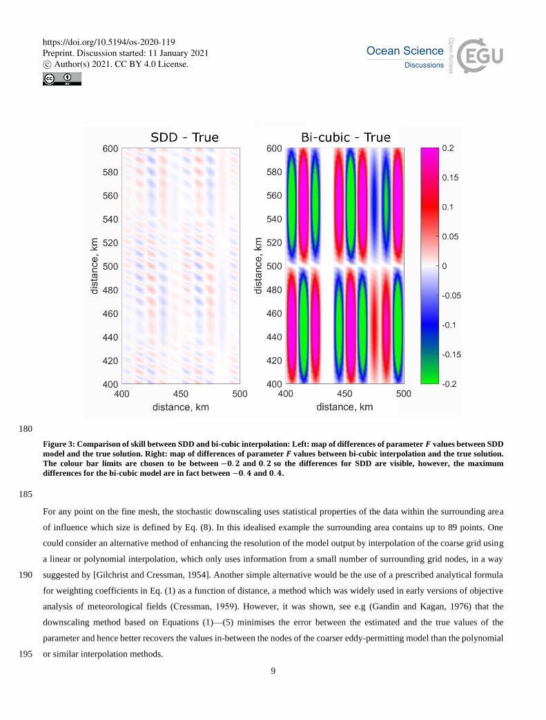
Figure 3: Comparison of skill between SDD and bi-cubic interpolation: Left: map of differences of parameter 𝑭 values between SDD

model and the true solution. Right: map of differences of parameter 𝑭 values between bi-cubic interpolation and the true solution.

The colour bar limits are chosen to be between −𝟎. 𝟐 and 𝟎. 𝟐 so the differences for SDD are visible, however, the maximum

differences for the bi-cubic model are in fact between −𝟎. 𝟒 and 𝟎. 𝟒.

185

For any point on the fine mesh, the stochastic downscaling uses statistical properties of the data within the surrounding area

of influence which size is defined by Eq. (8). In this idealised example the surrounding area contains up to 89 points. One

could consider an alternative method of enhancing the resolution of the model output by interpolation of the coarse grid using

a linear or polynomial interpolation, which only uses information from a small number of surrounding grid nodes, in a way

suggested by [Gilchrist and Cressman, 1954]. Another simple alternative would be the use of a prescribed analytical formula 190

for weighting coefficients in Eq. (1) as a function of distance, a method which was widely used in early versions of objective

analysis of meteorological fields (Сressman, 1959). However, it was shown, see e.g (Gandin and Kagan, 1976) that the

downscaling method based on Equations (1)—(5) minimises the error between the estimated and the true values of the

parameter and hence better recovers the values in-between the nodes of the coarser eddy-permitting model than the polynomial

or similar interpolation methods. 195


10

This example gives a quantitative estimate of how much improvement can be achieved by using the SDD method instead of

interpolation based on analytical formula. Fig. 2 shows the results produced by the SDD model in comparison with the true

solution and two polynomial interpolating models (bi-linear and bi-cubic) along a zonal transect located as shown in Fig. 1.

The maps of differences between the true solution, SDD and the bi-cubic model are shown in Fig. 3. All data are sampled on

the high-resolution grid. The SDD model is able (i) to recover the extremes missed in the parent, linear interpolating and bi-200

cubic interpolating models and (ii) generate a solution that is much closer to the exact one. The root-mean-square error

produced by the SDD model is only 0.008 while the error produced by the bi-cubic interpolating model is approximately 20

times higher at 0.177. The SDD method is computationally efficient; it takes only a few seconds to run the high-resolution

model on a small laptop for a 1000 km × 1000 km domain in this idealised setting.

2.3 Stochastic Model of the Red Sea 205

In this section the SDD method is applied to create a high resolution, eddy-resolving model of the Red Sea (SMORS) based

on the medium-resolution, eddy-permitting parent model. The parent model used in the study is PSY4V3R1, which is part of

the Mercator Global Ocean Analysis and Forecast System based on NEMO v 3.1. The parent model assimilates observational

data and has a medium 1/12th degree resolution with 50 depth levels (CMEMS, 2020). The outputs from this model are freely

available as Copernicus Marine Environment Monitoring Service product 210

GLOBAL_ANALYSIS_FORECAST_PHY_001_024 (hereafter called PHY_001_024). This product contains daily 10-day

forecasts of U- and V-components of current velocities, Temperature and Salinity in 3D and hourly outputs of temperature and

currents at the surface in 2D. In addition to the currents produced by PSY4V3R1, the surface hourly currents include tidal

streams and Stokes drifts. The output data are interpolated from the native staggered Arakawa C-grid onto an A-grid. SMORS

uses higher resolution bathymetry obtained from the 30 arc-second grid (GEBCO, 2014). The coastline and the land masks at 215

each depth level are obtained from the bathymetry data.

The SMORS downscaling model has a 1/24th degree horizontal resolution. We have developed two versions of SMORS: (i)

SMORS-3D uses 3D daily outputs from PHY_001_024 as its input, and (ii) SMORS-2D uses surface data from PHY_001_024

with hourly temporal resolution. SMORS takes medium resolution data from PHY_001_024 and uses the SDD techniques to

calculate all variables on a high-resolution mesh. The computational mesh for both versions of SMORS have a 1/24th degree 220

resolution and hence they quadruple the number of nodes of the original CMEMS grid in the horizontal dimensions. The

meshes are aligned in such a way that one out of four nodes in the high-resolution grid is shared with the medium-resolution

one. Both versions of SMORS can work operationally 24/7, and provide the same temporal resolution and length of forecast

as the parent medium-resolution model. As SMORS is an operational model, it polls periodically the Copernicus server using

Copernicus MOTU library for Python, until the new daily forecasting data are available. Once new data are found, they are 225

automatically downloaded into the local server.


11

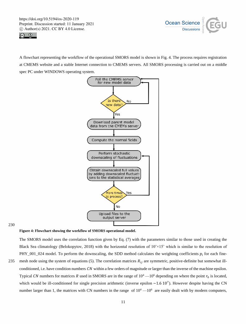
A flowchart representing the workflow of the operational SMORS model is shown in Fig. 4. The process requires registration

at CMEMS website and a stable Internet connection to CMEMS servers. All SMORS processing is carried out on a middle

spec PC under WINDOWS operating system.

230

Figure 4: Flowchart showing the workflow of SMORS operational model.

The SMORS model uses the correlation function given by Eq. (7) with the parameters similar to those used in creating the

Black Sea climatology (Belokopytov, 2018) with the horizontal resolution of 10’×15’ which is similar to the resolution of

PHY_001_024 model. To perform the downscaling, the SDD method calculates the weighting coefficients 𝑝𝑖 for each fine-

mesh node using the system of equations (5). The correlation matrices 𝑅𝑖𝑗 are symmetric, positive-definite but somewhat ill-235

conditioned, i.e. have condition numbers 𝐶𝑁 within a few orders of magnitude or larger than the inverse of the machine epsilon.

Typical 𝐶𝑁 numbers for matrices 𝑅 used in SMORS are in the range of 104 —106 depending on where the point 𝑟0 is located,

which would be ill-conditioned for single precision arithmetic (inverse epsilon ~1.6 107). However despite having the CN

number larger than 1, the matrices with CN numbers in the range of 104 —106 are easily dealt with by modern computers,


12

and hence can be considered fairly well conditioned for the double precision accuracy (64-bit) used in the computations 240

(inverse epsilon ~1016).

The numerical difficulties in using ill-conditioned correlation matrices can be reduced by applying advanced numerical

methods, for example Tikhonov method of variational regularisation (Tikhonov,1963), see also (Reichel and Yu, 2015) The

detailed algorithm of regularisation with practical examples is described in (Ryabov et al, 2018). After regularisation, a

standard method can be used for solving Eq (5). In case of SMORS, the solution of Eq. (5) does not result in any significant 245

loss of accuracy if all computations are performed with 64-bit precision.

Solving Eq. (5) for all 𝑝𝑖 and for every node in the high-resolution 3D grid is a computationally demanding task and requires

the use of highly efficient algorithms. For solving these equations, we have tried three methods: Gaussian elimination,

Cholesky decomposition and the conjugate gradient. We have found that the latter is the best choice in terms of speed and

numerical stability, if a suitable initial guess is provided, even if no special preconditioner is used. Since 𝑅 has values equal to 250

one in the diagonal, it can be considered as having a diagonal preconditioner. For the conjugate gradient solver, we have used

the code provided by Eigen C++ library (Guennebaud el al., 2020).

For a regular medium grid, the weighting coefficients only depend on the geometry of the grid and the correlation function,

therefore they could be computed just once, in advance. The geometry of the grid around fine-mesh points varies significantly

in many areas of the Red Sea due to highly variable bathymetry, multiple small islands, and a convoluted coastline. For the 255

initial guess in the iteration process, we use the solution found for the previously considered node (cut to size or padded with

zeros if the number of nodes is different). This approach takes advantage of the fact that both the medium and fine grids are

structured and therefore, in most cases, the weights for the neighbouring nodes are similar in value. With this approach, Eq.

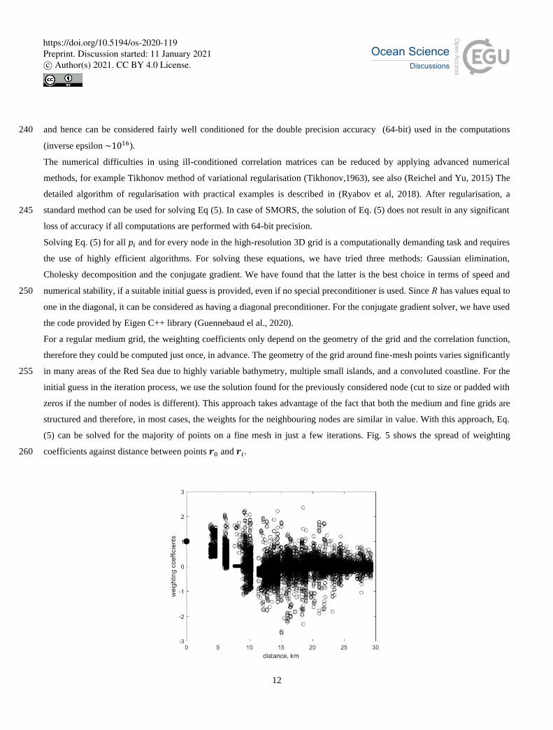
(5) can be solved for the majority of points on a fine mesh in just a few iterations. Fig. 5 shows the spread of weighting

coefficients against distance between points 𝒓0 and 𝒓𝑖. 260


13

Figure 5: Distribution of the weights 𝒑𝒊 against the distance ‖𝒓𝟎 − 𝒓𝒊‖. They are computed between the node on the fine mesh 𝒓𝟎 and

those points on the medium mesh which are used for calculation of the correlation matrix 𝒓𝒊. The plot includes approximately 2.5

million weights calculated for all the fine mesh nodes at the surface of the Red Sea. 265

After the weighting coefficients 𝑝𝑖 for each fine-mesh node have been found, the downscaling calculation for each fine-mesh

node for each parameter at each time point requires a minimum of 2𝑛 floating point operations, see Eq (1), where 𝑛 is the

number of surrounding medium-mesh points considered for use in downscaling. However, the most time consuming part of

calculation is not the calculation of high-resolution values according to Eq (1) but the calculation of weighting coefficients 𝑝𝑖

from the system of equations (5) as described above. 270

2.4 Model Validation

Many deterministic high-resolution models, both in oceanography and meteorology, are prone to errors caused by the so called

‘double penalty’ issue. The result of this issue is that higher resolution models have a larger root-mean-square-error (RMSE)

than lower resolution models (Gilleland et al. 2009). ‘Double penalty’ is related to the phenomenon where a model that predicts

some spatial feature, but slightly shifted, gets a worse RMSE than a coarser model that completely fails to predict that feature. 275

The physics of the double penalty issue has been studied in detail in (Zingerlea and Nurmib, 2008; ECMWF,2020; Haben et

al., 2014). They state, in relation to meteorological forecasts, that ‘High-resolution NWP models commonly produce forecasts

with seemingly realistic small-scale patterns that can be somewhat misplaced. Traditional point matching verification measures

(e.g. the root mean square error, RMSE) would penalize such misplacements very heavily. This penalization actually occurs

twice, first, for not having the pattern where it should be, and second, for having a pattern where there should not be one. To 280

the contrary, in the SDD method, the high-resolution output is nudged to the parent model, hence the phase shift and ‘double

penalty’ error is less likely.

The quality of SMORS has been assessed in two ways. First, the SMORS model output was validated by comparing the model

outputs with in-situ observations from ARGO floats (Coriolis, 2020) and sea-surface temperature from the Operational Sea

Surface Temperature and Sea Ice Analysis (OSTIA, 2020). OSTIA uses satellite data from a number of sensors as well as in-285

situ data from drifting and moored buoys. Validation routine follows the guidance produced by GODAE Ocean View

consortium (2020)

As an example, Fig. 6 shows the domain-averaged monthly bias and RMSE of SST between PHY_001_024 and OSTIA as

well as between SMORS_3D and OSTIA for the year 2016. Both models show a very similar skill with the bias between 0.01

oC and 0.31 oC, and the RMSE between 0.37 oC and 0.68 oC depending on the month. The differences in errors produced by 290

SMORS and the parent model are very small and their maximum values do not exceed 0.02 oC, both for bias and RMSE.

Therefore, no ‘double penalty’ issue is seen here.


14

Figure 6: Monthly RMSE and bias comparisons: Monthly RMSE (left panel) and monthly bias (right panel) between PHY_001_024

and OSTIA (red line); and between SMORS and OSTIA (black line). 295

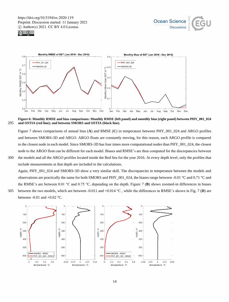
Figure 7 shows comparisons of annual bias (A) and RMSE (C) in temperature between PHY_001_024 and ARGO profiles

and between SMORS-3D and ARGO. ARGO floats are constantly moving, for this reason, each ARGO profile is compared

to the closest node in each model. Since SMORS-3D has four times more computational nodes than PHY_001_024, the closest

node to the ARGO float can be different for each model. Biases and RMSE’s are then computed for the discrepancies between

the models and all the ARGO profiles located inside the Red Sea for the year 2016. At every depth level, only the profiles that 300

include measurements at that depth are included in the calculations.

Again, PHY_001_024 and SMORS-3D show a very similar skill. The discrepancies in temperature between the models and

observations are practically the same for both SMORS and PHY_001_024, the biases range between -0.01 °C and 0.71 °C and

the RMSE’s are between 0.01 °C and 0.75 °C, depending on the depth. Figure 7 (B) shows zoomed-in differences in biases

between the two models, which are between -0.011 and +0.014 °C , while the differences in RMSE’s shown in Fig. 7 (D) are 305

between -0.01 and +0.02 °C.


15

Figure 7: Annually averaged biases (A) and RMSE’s (C) of temperature for the two models: PHY_001_024 – ARGO (dashed line)

and SMORS-3D – ARGO (solid line). Plots (B) and (D) show the zoomed-in differences between the lines in plots (A) and (C)

respectively. 310

The second test was to assess if the SDD method produces noise at high frequencies (in spatial domain). Theoretically, the

downscaling onto any existing ‘observational’ point (in this case a point on the PHY_001_024 mesh) must give exactly the

same value as the original data set (Gandin 1963, 1965). Any deviation from this rule is due to computational errors. These

errors were assessed as follows. The output surface data for 𝑢 and 𝑣 velocity components from SMORS were subsampled onto

the PHY_001_024 mesh and comparison was made by calculating the standard deviation of differences (std_DIF_u, and 315

std_DIF_v). The downscaling was carried out based on daily outputs from PHY_001_024 for each day of the year 2017. Both

values, std_DIF_u and std_DIF_v, were very small, of the order 10-8 m/s, while the typical velocities in the Red Sea were of

the order of 0.1—0.2 m/s. Therefore, the potential ‘double penalty’ error does not occur in the downscaling of profiles.

3 Results

High resolution reveals more intricate granularity and provides important information of smaller-scale processes, in 320

particularly those dependent of the gradients of the simulated variables. It is known that gradients of noisy data can have

greater errors than the variables themselves, see e.g. (Brekelmans et al, 2003). Hence, the higher resolution models should

ideally have better absolute accuracy than the coarser resolution models for the study of such properties as flow vorticity or

geopotential gradients related to geostrophic currents. The idealised experiments shown above demonstrate that SDD model

not only reveals more small-scale features, it also improves the accuracy of simulation. 325

In this section, the results produced by eddy-resolving SMORS-3D model for the year 2017 at the surface are analysed and

compared with the eddy-permitting product PHY_001_024 (3D output). The focus of this section is on dynamic properties

depending on the currents rather than temperature and salinity, as it is the dynamics where the most significant improvement

from downscaling is identified. The Red Sea is known for its mesoscale activity leading to the formation of eddies and

filaments, see e.g. (Zhai and Bower, 2013). In order to analyse mesoscale activity, the horizontal velocity 𝑈, 𝑉 is split into 330

slow varying components ⟨𝑈⟩ , ⟨𝑉⟩ representing mean currents and fluctuation components 𝑢 , 𝑣 representing mesoscale

activity:

𝑈 = ⟨𝑈⟩ + 𝑢, 𝑉 = ⟨𝑉⟩ + 𝑣, (10)

where the angle brackets designate statistical mean. As usual, we apply the assumptions of ergodicity and statistical

homogeneity of horizontal turbulence generated by mesoscale motions, and for practical purposes we estimate the statistical 335

mean by time averaging for each grid node. The slow varying components are calculated using a low-pass Savitzky-Golay

filter of the second order. The cut-off period is taken to be 𝑊 = 73 days as it provides a good separation of fast and slow

motion. For each geographical location we calculate the eddy kinetic energy, EKE, and the mean kinetic energy, MKE per unit

mass of water as follows


16

MKE =1

2[⟨𝑈⟩2 + ⟨𝑉⟩2], EKE =

1

2[⟨𝑢2⟩ + ⟨𝑣2⟩], (11) 340

where slow and fast velocities are defined by Eq (10). In order to assess the degree of separation between slow and fast motions,

and the validity of the ergodic assumption, we assess the cross-correlation term ⟨𝑈𝑢⟩ + ⟨𝑉𝑣⟩. Ideally, this term should be zero,

as part of the so called Reynolds conditions (Monin and Yaglom, 1971), and hence the following condition must be satisfied:

⟨FKE⟩ = MKE + EKE, (12)

where 345

⟨FKE⟩ =1

2[⟨𝑈2⟩ + ⟨𝑉2⟩],

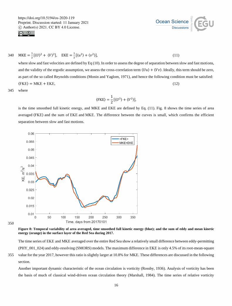
is the time smoothed full kinetic energy, and MKE and EKE are defined by Eq. (11). Fig. 8 shows the time series of area

averaged ⟨FKE⟩ and the sum of EKE and MKE. The difference between the curves is small, which confirms the efficient

separation between slow and fast motions.

350

Figure 8: Temporal variability of area averaged, time smoothed full kinetic energy (blue); and the sum of eddy and mean kinetic

energy (orange) in the surface layer of the Red Sea during 2017.

The time series of EKE and MKE averaged over the entire Red Sea show a relatively small difference between eddy-permitting

(PHY_001_024) and eddy-resolving (SMORS) models. The maximum difference in EKE is only 4.5% of its root-mean-square

value for the year 2017, however this ratio is slightly larger at 10.8% for MKE. These differences are discussed in the following 355

section.

Another important dynamic characteristic of the ocean circulation is vorticity (Rossby, 1936). Analysis of vorticity has been

the basis of much of classical wind-driven ocean circulation theory (Marshall, 1984). The time series of relative vorticity


17

averaged over the whole Red Sea and calculated from the outputs of the parent model (PHY_001_024) and SMORS is shown

in Fig. 9. Absolute values of vorticity calculated at individual grid points from the high resolution model are typically higher 360

than from the medium-resolution model. Higher values of vorticity are a result of better representation of horizontal gradients

in velocity by higher-resolution SMORS model. This effect is seen in both slow and fast varying components of vorticity. The

difference in the area averaged vorticity is a result of differences in the shape of the coastline and a number of islands

represented in the coarse and fine grids.

365

Figure 9: Area averaged vorticity as a function of time calculated from PHY_001_024 (black) and SMORS (red).

The difference in vorticity sampled on the coarser PHY_001_024 grid is shown in Fig. 10. The root mean square of the

difference (RMS-DV) in vorticity calculated over the entire Red Sea is smaller but comparable with RMS-V of the vorticity 370

itself. In the example shown in Fig. 10, the percentage ratio of the two is as high as 17%. The difference is larger in the areas

of intensive mesoscale activity in the central and northern parts of the Red Sea where the coarser PHY_001_024 model

underestimates velocity gradients.

375


18

Figure 10: Snapshot of a difference in the surface current vorticity (s−𝟏) calculated from SMORS and PHY_001_024 models for the

1st of April 2017.

An important dynamic characteristic of the mesoscale activity is the local enstrophy defined as the square of relative vorticity 380

at a location and the total enstrophy defined as an integral of local vorticity over the horizontal dimensions of a domain

Enstr(𝑡) = ∫ ‖∇ × 𝑼(𝑥, 𝑦, 𝑡)‖2𝑑𝐴Red Sea

. (13)

In the inviscid flow, enstrophy is conserved in a closed system, and hence variation of area averaged (or area integrated)

enstrophy gives an indication of the role of ocean-atmosphere interaction and viscous dissipation (Lesieur, 2008). The value

of enstrophy is also indicative of the rate of dissipation of kinetic energy, and hence a correct estimate of enstrophy provides 385

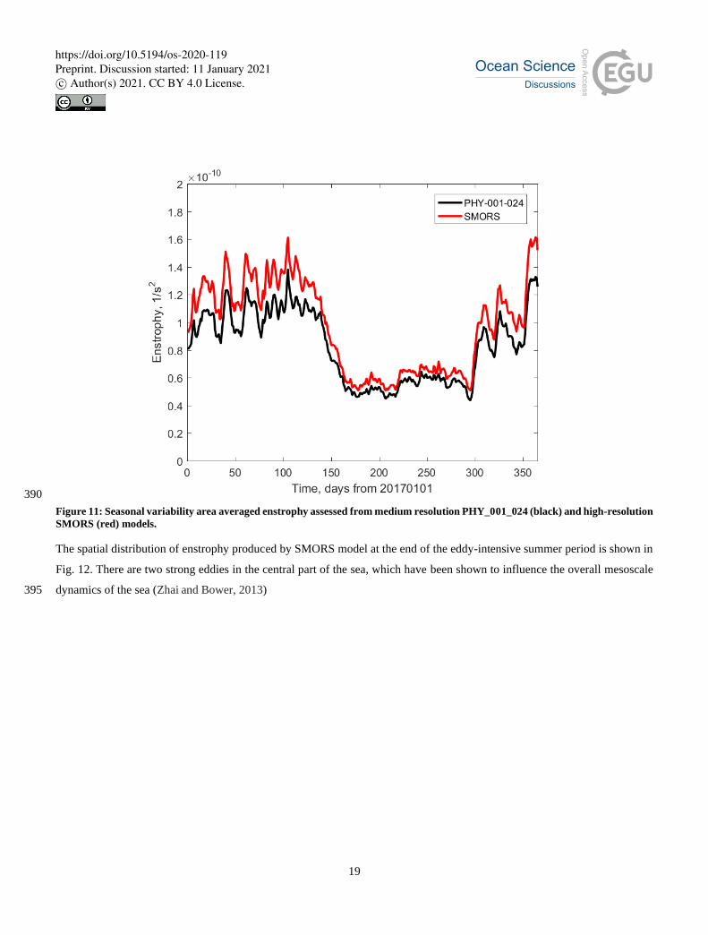
a better insight into the underlying processes of transformation of energy in the basin. The time series of area averaged

enstrophy, i.e. integral enstrophy defined by Eq. (13) divided by the area of the domain, is represented in Fig. 11. Enstrophy

is minimal in the summer period when mesoscale activity is reduced.


19

390

Figure 11: Seasonal variability area averaged enstrophy assessed from medium resolution PHY_001_024 (black) and high-resolution

SMORS (red) models.

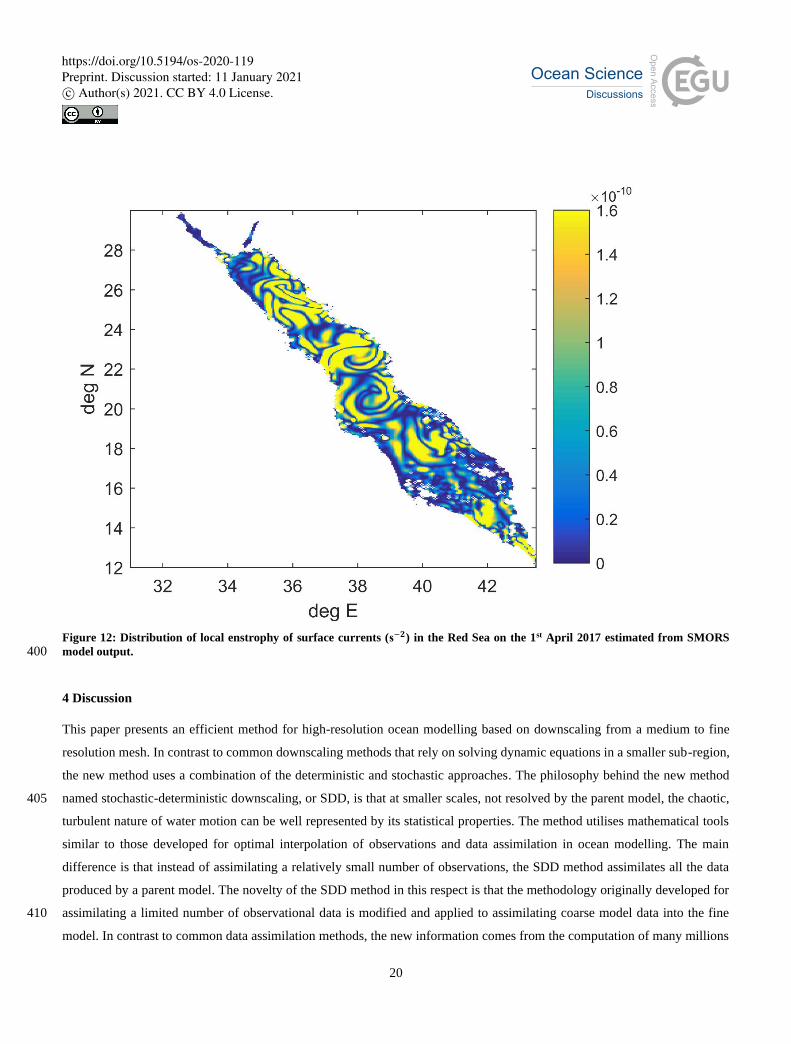
The spatial distribution of enstrophy produced by SMORS model at the end of the eddy-intensive summer period is shown in

Fig. 12. There are two strong eddies in the central part of the sea, which have been shown to influence the overall mesoscale

dynamics of the sea (Zhai and Bower, 2013) 395


20

Figure 12: Distribution of local enstrophy of surface currents (s−𝟐) in the Red Sea on the 1st April 2017 estimated from SMORS

model output. 400

4 Discussion

This paper presents an efficient method for high-resolution ocean modelling based on downscaling from a medium to fine

resolution mesh. In contrast to common downscaling methods that rely on solving dynamic equations in a smaller sub-region,

the new method uses a combination of the deterministic and stochastic approaches. The philosophy behind the new method

named stochastic-deterministic downscaling, or SDD, is that at smaller scales, not resolved by the parent model, the chaotic, 405

turbulent nature of water motion can be well represented by its statistical properties. The method utilises mathematical tools

similar to those developed for optimal interpolation of observations and data assimilation in ocean modelling. The main

difference is that instead of assimilating a relatively small number of observations, the SDD method assimilates all the data

produced by a parent model. The novelty of the SDD method in this respect is that the methodology originally developed for

assimilating a limited number of observational data is modified and applied to assimilating coarse model data into the fine 410

model. In contrast to common data assimilation methods, the new information comes from the computation of many millions


21

of downscaling factors, see Eq (5) and Fig. 5, which in turn uses the correlation matrices. Therefore, the SDD method should

be treated as experimental at this stage. The SDD approach is first applied to and tested in an idealised case and then applied

to create an operational Stochastic Model of the Red Sea, or SMORS, based on data available via Copernicus Marine

Environment Monitoring Service. SMORS has a 1/24th degree of resolution, compares favourably with observations, and 415

allows to reveal greater granularity of the dynamical features of the Red Sea, in particular those dependent on the shear of

ocean currents.

The statistical links used by the SDD method can be interpreted in a way similar to the theory of fully developed turbulence.

According to the Kolmogorov’s law the statistically uniform and isotropic (in 3D) turbulence can be described by a universal

power density spectrum (the law of 5/3) which is equivalent to the law of 2/3 for the structure functions (Gandin and Kagan, 420

1976). The studies of velocity fluctuation in the upper air showed that the correlation function for geopotential heights has a

universal shape for distances large enough to consider the processes to be 2-dimensional (in the horizontal) but smaller than

the Rossby radius of deformation (Yudin, 1961). Previous studies confirmed that the small-scale velocity fluctuations in well-

developed turbulence exhibit universal scaling properties independent of the large-scale flow structures (Nelkin, 1994).

The correct identification of the correlation function and, in particular, its digital representation in the form of the correlation 425

matrix R given by Eq. (6) is critical for the success of the SDD method. Theoretically, matrix R should be symmetric and

positive-definite, however this is not always the case when the matrix is derived from observations (Tabeart et al., 2020).

There are a number of ways to estimate the numerical values of elements in the correlation matrix (6), see e.g. (Park and Xu,

2018; Fu et al., 2004). For the purpose of downscaling, an optimal design of matrix R would ideally be optimised to reflect the

structures at a short range, comparable with the resolution of the parent model. It has been shown that the dependence of the 430

autocorrelation matrix on the horizontal distance ‖𝒓𝑖 − 𝒓𝑗‖ is universal at small separations and is close to universal at

separation comparable to Rossby radius of deformation (Yudin,1961, Gandin, 1963). This is consistent with a general view

that the Rossby radius is a predominant scale for coherent structures in the ocean such as mesoscale eddies, which are typically

2—3 times larger than the first baroclinic Rossby radius, see e.g. (Beron-Vera et al, 2019; Badin et al, 2009).

Whilst the elements of the correlation matrix 𝑅𝑖𝑗 depend only on the distance between the contributing points as specified by 435

Eq (7), the weighting coefficients 𝑝𝑖 are not a unique function of the distance between the points 𝑟0 and 𝑟𝑖. This means that

standard interpolation methods such as bi-linear, polynomial, inverse distance etc. based on a fixed dependence of weights on

distance cannot be used as an adequate substitution to the method described above, as this method minimises the error between

the true and estimated values on the fine mesh (Gandin, 1965) and hence it gives the best possible estimates of ocean

parameters. The distribution of weights is generally different for different points 𝑟0 on the fine mesh, however it may be the 440

same for a subset of points away from the coastlines due to the regular structure of the medium mesh.

In theory, in order to solve the 𝑁fine systems of equations (5) for each node on the fine mesh, the matrix 𝑅𝑖𝑗 has to involve all

the nodes of the medium mesh in the domain, because eq. (7) gives values of 𝑅𝑖𝑗 different from zero, no matter what is the

distance between nodes. In practice, this is undesirable. Firstly, large systems of equations require vast computational resources


22

to be solved. Secondly, large correlation matrices are known to have large condition numbers (Tabeart et al., 2020) and this 445

problem gets worse as the matrix size increases. Thirdly, the data from nodes which are away by more than a few Rossby radii,

are not physically correlated to small scale variations within a single grid cell of the medium mesh.

The reason for matrix 𝑅 to be ill-conditioned is that whilst its largest elements (equal to 1) are on its diagonal, there are many

non-diagonal elements which have similar, however slightly smaller values. This is because the grid cell on the medium mesh

is smaller than a typical size of mesoscale features (2—3 times the Rossby radius). The Rossby radius determines the scale of 450

coherency of ocean parameters, therefore the correlations between neighbouring points on the medium mesh are close to 1.

The baroclinic Rossby radius in the Red Sea is about 10—30 km (Manasrah, 2006; Zhai and Bower, 2013). In principle, the

matrix 𝑅 could have been made more diagonally dominant and its condition number would have reduced if using a coarser

mesh. However, this would have led to the loss of statistical information at smaller scales and hence would introduce larger

errors in the downscaling process. 455

The SMORS model is a computationally efficient way to generate higher 3D oceanographic forecast for the Red Sea. With all

considerations listed above, the whole process of downloading the file from the Copernicus server, finding the weighting

coefficients, downscaling the fields of U, V, T and S, and saving the output NetCDF file, takes about three hours on a single

core of a typical desktop PC. Efficiency of SMORS model is seen from the following comparison. The time required for both

SMORS-3D and SMORS-2D to run on a desktop PC with a single core is comparable to the time required for a purely 460

deterministic model (such as NEMO) with the same resolution to run on a HPC cluster with 96 computing cores. If faster

speeds for the SDD method are needed, the algorithm is parallelizable on a modern desktop PC or, of course, on an HPC

cluster. The running of the model can be further optimised by applying the SDD method only to a selection of depth levels

used by the parent model, either horizontal or curved.

The SDD method was tested using an idealised case where the true solution is known (sub-section 2.2). The SDD method 465

showed good ability to recover smaller scale details of mesoscale eddies which were missed by the parent eddy-permitting

model, as well as high-resolution interpolating models based on a prescribed analytical formula for weighting coefficient. The

comparison of the maps and transects produced by the parent (coarse), analytical interpolating and SDD based models, see

sub-section ‘idealised case’ above, shows the benefits of the SDD method in comparison with downscaling approaches based

on analytical interpolation routines. The SDD method produces data on the fine mesh which are much closer to the true solution 470

than simple bi-linear or bi-cubic interpolation. In contrast to the analytical interpolation methods which smooth the gradients,

the SDD is capable of recovering sharp gradients and details of the ocean fronts. Similar qualities are seen in the real world

application of the SDD to the Red Sea, where SMORS model shows finer granularity of the velocity, vorticity and enstrophy

fields, than the parent model.

The high-resolution SMORS model not only provides a greater granularity of the spatial distribution that a coarser parent 475

model misses, it also gives different estimates for the area averaged ocean variables. For example, while the differences

between the full kinetic energy computed with the parent and fine-mesh models shown in Fig. 8 are relatively small, they can

be attributed to the ability of SMORS model to reveal local extrema in velocity which are not resolved by PHY_001_024. The


23

seasonal variation of EKE and MKE produced by SMORS shows lower mesoscale activity in summer and higher in winter,

similar to the results obtained with high-resolution deterministic model MITgcm (Zhan et al, 2016). 480

The knowledge of the structure and evolution of vorticity field in the ocean provides vital information about ocean circulation.

For example, the effect of mesoscale eddies is to produce a transport of vorticity from regions of high to regions of low vorticity

(Corre et al, 2020). Mesoscale flows are the primary cause for the ocean transport of heat, carbon and nutrients (Robinson,

1983). Furthermore, the sub-mesoscales (1 km—10 km) are emerging as an important dynamical regime. Dynamical processes

at the mesoscales and sub-mesoscales are relevant for understanding and modelling interactions near the coasts and the 485

movement of ocean heat under high latitude ice-shelves that can have important implications for sea level (GFDL, 2020). The

knowledge of vorticity values helps assess the stability of the 2D flow to 3D instabilities (Flor, 2010). Therefore, its accurate

calculation is a desired quality of any ocean circulation model.

Vorticity is closely linked to another important feature of the flow, its local enstrophy. The SMORS model reveals high level

of granularity in enstrophy distribution in particular north and south of the persistent eddies in the central part of the Red Sea 490

as shown in Fig. 13 which demonstrates the spatial distribution of differences in enstrophy computed by SMORS and

PHY_001_024. The difference in vorticity and enstrophy is a result of the fact that the velocity gradients in the high-resolution

child model are sharper than in the parent model. This effect is clearly seen in the idealised case, where the true solution was

known (see sub-section 2.2 ‘Idealised case’). Hence, the enstrophy is nearly always higher in the high-resolution model. The

difference between the models can be characterised by the ratio of root-mean-square of difference in enstrophy to the root-495

mean-square of enstrophy itself which is as high as 21% for the snapshot shown in Fig. 13.


24

500 Figure 13: Spatial distribution of differences in surface enstrophy (𝒔−𝟐) between the high-resolution and medium-resolution models

on the 1st of April of 2017.

The benefits of the higher-resolution model are better seen in a zoomed-in area shown in Fig. 14. The high-resolution model

provides better granularity and it also better resolves the maxima in enstrophy which were not resolved by the parent medium

resolution model. 505


25

Figure 14: Enstrophy of surface currents in the central part of the Red Sea presented by eddy-permitting PHY_000_024 (left) and

eddy resolving SMORS (right) model: The white areas represent land and are different as the fine model uses higher resolution

bathymetry and coastline, which reveals more small islands. 510

5 Conclusion

We present an efficient method for high-resolution ocean modelling which uses downscaling from a medium resolution model

and is based on the combination of the deterministic and stochastic approaches. We call this method stochastic-deterministic

downscaling, or SDD. The philosophy behind SDD is that at smaller scales the chaotic, turbulent nature of water motion can

be represented more efficiently by incorporating methodologies commonly used in the study of turbulence. The method utilises 515

the same mathematical tools which were originally developed for optimal interpolation of observational data in meteorology

and then for data assimilation in ocean modelling. The main difference is that instead of assimilating a relatively small number

of observations, the SDD method assimilates a vast number of gridded data produced by a parent model. The SDD model has

the same length of forecast, vertical discretisation and frequency of outputs as the parent model. The method can be applied to

individual depth levels independently. 520

The validation of SDD in an idealised setting, where the exact solution is known, demonstrates its ability to reconstruct finer-

scale features which are lost in the parent lower resolution model. The method is shown to be efficient in case where the parent

model is eddy-permitting, while the downscaled model is eddy-resolving. The SDD type model named SMORS (Stochastic

Model of the Red Sea) was set up for the Red Sea with a resolution of 1/24o using a parent model from Copernicus Marine

Environmental Service with 1/12o degree resolution and ran operationally for more than a year. Validation against the parent 525

model, in-situ and satellite observations confirmed that SDD is not prone to generating additional errors due to the ‘double-

penalty’ effect which is common for purely deterministic high-resolution models.

The SMORS model uses advanced numerical algorithms, is computationally efficient and can be run on a single core of a

desktop PC operationally. The running of the model can be further optimised by applying the SDD method only to a selection


26

of depth levels used by the parent model, either horizontal or curved. It is likely that the method could be further developed by 530

incorporating more complex data assimilation schemes.

Author contribution

GS conceptualised and designed the study, performed the analysis, and drafted the manuscript.

JO created numerical schemes, carried out software development, contributed to the analysis and writing the manuscript. VB

contributed to the development of the algorithm and selection of appropriate parameters. 535

Competing interests

The authors declare that they have no conflict of interest.

Acknowledgment

Funding for this study was provided by the University of Plymouth Enterprise LTD. The authors are thankful to Xavier Francis

for his help in the validation of the earlier version of SMORS. 540

References

Badin, G., Williams, R. G., Holt, J. T. and Fernand, L. J.: Are mesoscale eddies in shelf seas formed by baroclinic instability

of tidal fronts? J. Geophys. Res., Vol. 114, C10021, doi:10.1029/2009JC005340, 2009.

Barth A., Azcárate, A. A., Joassin, P., Beckers, J-M., Troupin,C.: Introduction to Optimal Interpolation and Variational

Analysis, SESAME Summer School, Varna, Bulgaria, 2008. 545

Belokopytov, V.N.: Retrospective Analysis of the Black Sea Thermohaline Fields on the Basis of Empirical Orthogonal

Functions. J. Phys. Oceanogr, 25 (5), pp. 380-389. doi:10.22449/1573-160X-2018-5-380-3, 2018.

Beron-Vera, F. J., Hadjighasem, A., Xia, Q., Olascoaga, M. J. and Haller, G:. Coherent Lagrangian swirls among submesoscale

motions, Proc. Natl. Acad. Sci. U.S.A, vol. 116 ,no. 37 ,18251–18256, 2019.

Boyer, T.P., S. Levitus, H. Garcia, R.A. Locarnini, C. Stephens, J. Antonov: Objective analyses of annual, seasonal, and 550

monthly temperature and salinity for the world ocean on a 0.25° grid. Int. J. Climatol. 25: 931–945. DOI: 10.1002/joc.1173,

2005.

Brekelmans R., Driessen L., Hamers H. and Hertog D.: Gradient Estimation Schemes for Noisy Functions. J. Optim. Theory

Appl., 126, pages 529–551. doi: 10.1007/s10957-005-5496-2, 2005.

Bretherton, F. P., Davis, R. E., & Fandry, C. B.: A technique for objective analysis and design of oceanographic experiments 555

applied to MODE-73. Deep-Sea Research, 23, 559-582. doi:10.1016/0011-7471 (76)90001-2, 1976


27

Bruciaferri D., Shapiro G. I., Stanichny S., Zatsepin A., Ezer T., Wobus F., Francis X. and Hilton D.: The development of a

3D computational mesh to improve the representation of dynamic processes: The Black Sea test case. Ocean Model., 146,

101534. doi: 10.1016/j.ocemod.2019.101534, 2019

Bryan, K.: A numerical investigation of a nonlinear model of a wind-driven ocean. J. Atmos. Sci. 20, 594–606, 1963. 560

CMEMS: Copernicus Marine Environment Monitoring Service. https://marine.copernicus.eu [Accessed July 6, 2020].

Coriolis: Coriolis operational oceanography. http://www.coriolis.eu.org [Accessed July 6, 2020].

Corre M.L., Gula G., and Tréguier A.-M.: Barotropic vorticity balance of the North Atlantic subpolar gyre in an eddy-resolving

model. Ocean Science. 16, 451–468, 2020. doi: 10.5194/os-16-451-2020, 2020.

Cressman, G.P.: An Operational Objective Analysis System. Mon. Weather Rev, 87, 367-374. http://dx.doi.org/10.1175/1520-565

0493(1959)087<0367:AOOAS>2.0.CO;2, 1959

Dobricic, S., Pinardi, N.: An oceanographic three-dimensional variational data assimilation scheme. Ocean Modelling 22, 89–

105, 2008

Dobricic, S., Pinardi, N., Adani, M., Tonani, M., Fratianni, C. et al.: Daily oceanographic analyses by Mediterranean

Forecasting System at the basin scale. Ocean Science, 3 (1), 149-157, 2007 570

ECMWF,2020. https://confluence.ecmwf.int/display/FUG/12.A+Statistical+Concepts+-+Deterministic+Data#id-

12.AStatisticalConceptsDeterministicData-The%C2%93%E2%80%9CDoublePenaltyEffect%C2%94%E2%80%9D ,

accessed 05.01.2021.

Ezer, T., and Mellor, G. L.: A generalized coordinate ocean model and a comparison of the bottom boundary layer dynamics

in terrain-following and in z-level grids. Ocean Model. 6, 379–403. doi: 10.1016/S1463-5003(03)00026-X, 2004 575

Fletcher S.J.: Data Assimilation for the Geosciences: From Theory to Application, Elsevier; 919 pp, ISBN: 0128044446, 2017

Flor J.-B. (Ed.): Fronts, Waves and Vortices in Geophysical Flows, Lecture Notes in Physics 805. Springer, Berlin,

Heidelberg, doi 10.1007/978-3-642-11587-5, p.52, 2010

Fox-Kemper B, Adcroft, A., Böning, C. W., Chassignet, E. P., Curchitser, E., Danabasoglu, G. et al.: Challenges and Prospects

in Ocean Circulation Models, Front. Mar. Sci., 6, 65p, doi:10.3389/fmars.2019.00065, 2019. 580

Frisch, U.: Turbulence: The legacy of A. N. Kolmogorov., Cambridge University Press, 296 p., ISBN 0-521-45103-5, 1995

Fu, W., Zhou, G., Wang, H.: Ocean Data Assimilation with Background Error Covariance Derived from OGCM Outputs, Adv

Atmos Sci, vol. 21, no. 2, 181–192, 2004.

Gandin, L. S.: The problem of optimal interpolation, Scientific papers. Main Geophysical Observatory, vol 99, 1959. (In

Russian: Гандин Л. С., 1959. Задача об оптимальной интерполяции. Труды ГГО. вып. 99). 585

Gandin, L. S.: Objective analysis of meteorological fields. Leningrad, Gidrometeoizdat, 287 pp., 1963 (In Russian: Гандин,

Л. С., 1963. Объективный Анализ Метеорологических Полей. Ленинград , Гидрометеорологическое Издательство,

287 c.)

Gandin, L. S.: Objective analysis of meteorological fields. Translated from the Russian. Jerusalem, Israel Program for

Scientific Translations, 242 p., 1965 590


28

Gandin L.S. and Kagan R.L.: Statistical methods for meteorological data interpretation, Leningrad, Gidrometeoizdat, 359 pp.

(In Russian: Гандин Л.С., Каган Р.Л , 1976. Статистические методы интерпретации метеорологических данных ,

Ленинград, Гидрометеоиздат 359 стр.)

GEBCO, 2014: The GEBCO_2014 Grid, version 20150318. www.gebco.net [Accessed July 6, 2020]

GFDL, 2020: https://www.gfdl.noaa.gov/high-resolution-modeling/. [Accessed July 6, 2020] 595

Gilleland, E., Ahijevych, D., Brown, B. G., Casati, B. and Ebert, E. E.: Intercomparison of spatial forecast verification methods.

Weather Forecast, 24(5), 1416-1430, 2009.

Gilchrist В., Cressman G. P.: An experiment in objective analysis. Tellus, 6. no. 4: 309-318, 1954.

GODAE OceanView, 2020. https://www.godae-oceanview.org/science/task-teams/intercomparison-and-validation-tt/

Grigoriev et al. Correlation structure of thermohaline fields in the Black Sea in summer season. Okeanologiya, 36 (3) 364-600

369, 1996. (In Russian:Григорьев А.В., Иванов В.А., Капустина Н.А., 1996 . Корреляционная структура термохалинных

полей Черного моря в летний сезон, Океанология. –– Т. 36, № 3. – С. 364–369

Guennebaud G. et al., 2020: http://eigen.tuxfamily.org/ [Accessed July 6, 2020]

Kolmogorov, A. N.: The Local Structure of Turbulence in Incompressible Viscous Fluid for Very Large Reynolds' Numbers.

Doklady Akademiia Nauk SSSR, vol.30, p.301-305, 1941. 605

Haben, S., Ward, J., Greetham, D.V., Singleton, C., Grindrod, P.,. A new error measure for forecasts of household-level,

high resolution electrical energy consumption. International Journal of Forecasting, 30 (2), pp 246-256, 2014

https://doi.org/10.1016/j.ijforecast.2013.08.002

Korotaev, G. K., Oguz, T., Dorofeyev, V. L., Demyshev, S. G., Kubryakov, A. I., Ratner, Yu. B.: Development of Black Sea

nowcasting and forecasting system Ocean Science, 7, 629–649, 2011. 610

Lesieur M.: Turbulence in Fluids, Springer, Dordrecht, 558pp, ISBN 978-1-4020-6434-0, 2008.

Lindsay, K.: A Newton–Krylov solver for fast spin-up of online ocean tracers. Ocean Model., 109, 33–43. doi:

10.1016/j.ocemod.2016.12.001, 2017.

Manasrah R., Lass H. U. And Fennel, W.: Circulation in the Gulf of Aqaba (Red Sea) during Winter–Spring. J. of Oceanogr,

Vol. 62, pp. 219-225, 2006. 615

Marshall, J. C.: Eddy-mean-flow interaction in a barotropic ocean model, Quart. J . R. Met. Soc.,110, pp. 573-590, 1984.

Miller, R. N.: Numerical Modeling of Ocean Circulation. Cambridge University Press; 242 pp.; ISBN: 978-0-521-78182-4,

2007.

Mirouze, I., Blockley, E.W., Lea , D.J., Martin, M.J., Bell, M. J.: A multiple length scale correlation operator for ocean data

assimilation. Tellus A: Dynamic Meteorology and Oceanography, 68:1, 29744, DOI: 10.3402/tellusa.v68.29744, 2016. 620

Monin, A. S. and Yaglom, A. M.: Statistical Fluid Mechanics, Volume 1. Mechanics of Turbulence MIT Press; 782 pages,

ISBN-10: 0262130629, 1971.

Nelkin, M.: Universality and scaling in fully developed turbulence, Adv. Phys., 43:2, 143-181, doi:

10.1080/00018739400101485, 1994.


29

OSTIA, 2020: Operational Sea Surface Temperature and Sea Ice Analysis. http://ghrsst-pp.metoffice.com/ostia/ [Accessed 625

July 6, 2020]

Park, S. K., Xu L. (Editors): Data Assimilation for Atmospheric, Oceanic and Hydrologic Applications (Vol. III), Springer,

592 pages, ISBN-10: 3319828185, 2018.

Reichel, L. and Yu, X.: Matrix Decompositions for Tikhonov Regularization. Electron. Trans. Numer. Anal.. vol. 43, pp. 223-

243, 2015. ISSN 1068-9613, 2015. 630

Robinson, A. R. (Ed.).: Eddies in marine science. Springer-Verlag Berlin Heidelberg. XXVI, 612pp, ISBN 978-3-642-69003-

7, 1983.

Rossby, C.-G.: Dynamics of Steady Ocean Currents in the Light of Experimental Fluid Mechanics. Papers in Physical

Oceanography and Meteorology, Vol.5, No1, 43 pp., 1936.

Ryabov et al.: On numerical solution of systems of linear algebraic equations with ill-conditioned matrices. International 635

Research Journal, No 12 (78) part 1, p 13-17. ISSN 2227-6017, 2018. (In Russian: Рябов В.М. , Бурова И.Г., Кальницкая

М.А., Малевич А.В. , Лебедева А.В., Борзых А.Н. О численном решении систем линейных алгебраических уравнений

с плохо обусловленными матрицами. Международный Научно-Исследовательский Журнал, No 12 (78) часть 1, стр.13-

17. DOI: https://doi.org/10.23670/IRJ.2018.78.12.002).

Smagorinsky, J.: General circulation experiments with the primitive equations: 1. The basic experiment., Monthly. Weather. 640

Review 91 (3): 99–164 , 1963

Tabeart, J. M., Dance, S. L., Lawless, A. S., Nichols, N. K., Waller, J. A.: Improving the condition number of estimated

covariance matrices, Tellus, series A: Dynamic Meteorology and Oceanography, 72:1, 1-19, DOI:

10.1080/16000870.2019.1696646, 2020.

Tennekes, H.; Lumley, J. L.: A first course in turbulence MIT Press. ISBN 978-0-262-20019-6, 1992. 645

Tikhonov A.N., 1963. (In Russian: Тихонов А. Н., О регуляризации некорректно поставленных задач, Докл. АН СССР,

1963, том 153, номер 1, 49–52)

Vasquez, T.: Objective Analysis, Digital Atmosphere, Weather Graphics Technologies, 2003.

http://www.weathergraphics.com/dl/daanal.pdf [Accesssed July 6, 2020]

Yudin, M.: Some regularities in the geopotential field, Scientific papers, Main Geophysical Observatory, vol 121, 1961. (In 650

Russian: Юдин М. И. 1961. Некоторые закономерности структуры поля геопотенциала. Труды ГГО, вып. 121).

Zhai, P. and Bower, A.: The response of the Red Sea to a strong wind jet near the Tokar Gap in summer. J. Geophys. Res.

Oceans, 118, 422–434, doi:10.1029/2012JC008444, 2013.

Zhan, P., Subramanian, A. C., Yao F., Kartadikaria, A. R., Guo, D. and Hoteit, I.: The eddy kinetic energy budget in the Red

Sea, J. Geophys. Res. Oceans, 121, doi:10.1002/2015JC011589, 2016. 655

Zingerlea, C., and Nurmib, P.: Monitoring and verifying cloud forecasts originating from operational numerical models,

Meteorological Applications, 15, pp. 325–330, 2008.


high resolution stochastic downscaling method for ocean

Documents