high resolution mapping of the magnetic field of the solar corona

H I G H R E S O L U T I O N M A P P I N G O F T H E M A G N E T I C F I E L D

O F T H E S O L A R C O R O N A

M A R T I N D. A L T S C H U L E R *

High Altitude Observatory, National Center for Atmospheric Research**, Boulder, Colo. 80303, U.S.A.

R A N D O L P H H. L E V I N E

Center for Astrophysics, Harvard College Observatory and Smithsonian Astrophysical Observatory,

Cambridge, Mass. 02138, U.S.A.

M I C H A E L STIX

Universitiits- Sternwarte, G6ttingen, F.R. G.

and

J O H N H A R V E Y

Kitt Peak National Observatory,? Tucson, Ariz. 85726, U.S.A.

(Received 14 April; in revised form 10 June, 1976)

Abstract. High resolution KPNO magnetograph measurements of the line-of-sight component of the photospheric magnetic field over the entire dynamic range from 0 to 4000 gauss are used as the basic data for a new analysis of the photospheric and coronal magnetic field distributions. The daily magnetograph measurements collected over a solar rotation are averaged onto a 180 x 360 synoptic grid of equal-area elements. With the assumption that there are no electric currents above the photospheric level of measurement, a unique solution is determined for the global solar magnetic field. Because the solution is in terms of an expansion in spherical harmonics to principal index n = 90, the global photospheric magnetic energy distribution can be analyzed in terms of contributions of different scale-size and geometric pattern. This latter procedure is of value (1) in guiding solar dynamo theories, (2) in monitoring the persistence of the photospheric field pattern and its components, (3) in comparing synoptic magnetic data of different observatories, and (4) in estimating data quality. Differ- ent types of maps for the coronal magnetic field are constructed (1) to show the strong field at different resolutions, (2) to trace the field lines which open into interplanetary space and to locate their photospheric origins, and (3) to map in detail coronal regions above (specified) limited photospheric areas.

1. Introduction

S o m e y e a r s ago , a m e t h o d was d e v e l o p e d to c a l c u l a t e t h e g l o b a l m a g n e t i c f ie ld o f

t h e so la r c o r o n a f r o m (1) m e a s u r e m e n t s of t h e l i n e - o f - s i g h t c o m p o n e n t of t h e

p h o t o s p h e r i c m a g n e t i c f ie ld ( c o l l e c t e d o v e r a so l a r r o t a t i o n ) , a n d (2) t h e a s s u m p -

t i o n tha t n o e l ec t r i c c u r r e n t s ex i s t a b o v e t h e l e v e l of t h e m e a s u r e d p h o t o s p h e r i c

Present address: Dept. of Computer Science, S.U.N.Y. at Buffalo, 4226 Ridge Lea Road, Amherst, N.Y. 14226, U.S.A. ** The National Center for Atmospheric Research is sponsored by the National Science foundation. t Kitt Peak National Observatory is operated by the Association of Universities for Research in Astronomy, Inc. Under contract with the National Science Foundation.

Solar Physics 51 (1977) 345-375. All Rights Reserved Copyright �9 1977 by D. Reidel Publishing Company, Dordrecht-Holland

346 M A R T I N D. A L T S C H U L E R E T AL.

field (Altschuler and Newkirk, 1969; Schatten, 1971a). This method provided a unique current-free (potential field) approximation to the actual but unknown coronal magnetic field.

Calculated distributions of the large-scale coronal magnetic field were compared (1) with the orientations of various coronal structures seen in white light above the limb (Newkirk and Altschuler, 1970; Newkirk, 1971; Schatten, 197 lb), (2) with coarse structures or intensity distributions observed at X-ray wavelengths above both the disk and the limb, (3) with the locations and propagation directions of radio sources and transients in the plane of the sky (Smerd and Dulk, 1971; Dulk et al., 1971), (4) with Moreton wave effects in the chromosphere under the MHD fast-mode coronal wave hypothesis (Uchida et al., 1973), and (5) with interplanetary magnetic fields and solar wind streams (Schatten et al., 1969). To assist such comparisons, Mt. Wilson magnetograph data were used to compute maps of both the strong and weak coronal magnetic fields for the period August 1959 to January 1974 (with occasional gaps when data were not available), and these maps were assembled into an Atlas (Newkirk et al., 1973).

The calculated magnetic fields of the Atlas often agreed (in location and configuration) with observed large-scale coronal structure and activity. Comparison of the Atlas maps with smaller scale coronal features, however, was not meaningful because the Atlas maps were derived from a spherical harmonic expansion truncated at principal index n = 9, and were thus severely limited in spatial resolution. Details of the coronal magnetic field smaller than about ~ of the solar circumference (or 240 Mm in the low corona) could not be discerned. Such coarse resolution washes out the coronal field structure of an entire active region. In practice this means that a comparison of the Atlas magnetic fields with many of the small but intense X-ray loops and arcades seen in the low corona is not useful.

High resolution mapping of the current-free coronal magnetic field above limited photospheric regions less than 200 Mm in size is possible with the Schmidt and other related programs (Schmidt, 1964; Levine, 1975). Magnetic maps derived by these methods have been compared with small-scale coronal structures (see for example, Rust and Roy, 1971). A difficulty in the use of such programs, however, is that boundary conditions must be specified at the edges of the limited photospheric region, and these boundary conditions are equivalent to assumptions about how neighboring photospheric regions contribute to the coronal magnetic field being calculated.

The primary purpose of our present work is to increase the resolution and reliability of the global-scale current-free coronal magnetic field maps. We want to increase resolution to such an extent that magnetic structures in the low corona as small as 25 Mm in size (that is, 2 ~ heliographic) can be traced in global context. (Still smaller structures are best studied on the basis of daily magnetograms.) To improve the reliability of the spherical harmonic analysis we use (1) data with a larger dynamical range (to 4000 gauss) so that less magnetic flux will escape our attention, and (2) a better computational algorithm. A second purpose (which is a

H I G H R E S O L U T I O N M A P P I N G O F T H E M A G N E T I C F I E L D 3 4 7

necessary step toward our primary goal) is to compute and store on magnetic tape the average CMP (central-meridian-passage) line-of-sight photospheric field for each area element of a 180• 360 synoptic data grid referenced to Carrington coordinates. In this format, a continual record of the photospheric magnetic field for an entire year can be stored on a single magnetic tape, and 28 day solar rotation periods with arbitrary initial and final dates can be analyzed. A tape library of the synoptic photospheric field to a 180 x 360 grid should be convenient for researchers in solar activity and solar dynamo theory who are interested in studying relatively long periods of time and who would have difficulty analyzing many daily magnetograph tapes. A third purpose is to store on magnetic tape for sequential solar rotations the spherical harmonic coefficients of the global photospheric field to principal index n = 90 (that is, 8281 coefficients for each rotation).

There are a number of reasons why we feel that the resolution and reliability of (current-free) coronal magnetic field maps should be greatly increased. First, new magnetographs can provide on a routine basis line-of-sight magnetic measurements with very high resolution ( - 1 Mm) and with linearity of signal to field over a large dynamical range (to 4000 gauss). Second, the increasing availability of mass storage devices on computers since our technique was first programmed in 1969 makes it possible to calculate economically many more terms in a spherical harmonic expansion. Third, the AS&E and Aerospace X-ray telescopes on Skylab have revealed interesting coronal structures too small for meaningful comparison with the calculated fields of the present coronal magnetic Atlas. Fourth, accurate mapping is needed over the entire dynamical range (0 to 4000 gauss) since important questions concern the weak fields of coronal holes as well as the strong fields above active regions. Fifth, the present use of Schmidt-type programs for high resolution restricted-area (non-global) coronal field mapping has inherent drawbacks especially when the region of interest cannot be isolated from surrounding active regions which exert considerable magnetic influence. With the technique presented here, accurate maps of the coronal potential field can be constructed above any small photospheric region without the need of guessing local boundary conditions.

We describe in Sections 3 through 6 the significant algorithmic and data handling improvements which have allowed us to extend the technique of Altschuler and Newkirk (1969) from a maximum principal index of n = 9 (with 100 coefficients including the magnetic monopole term) to n = 9 0 (with 8281 coefficients including the monopole term). This increase in the truncation limit of the series corresponds to roughly a ten-fold increase in linear resolution and a 100-fold increase in area resolution. With perfect data, a truncation limit of n = 90 permits detection of (current-free) magnetic structures in the low corona which are only 25 Mm in diameter. In Section 7 we illustrate the improved coronal magnetic mapping. A new type of global map which traces the open magnetic field back f r~ , l the corona to the photosphere is introduced. This map permits us to locate and estimate those photospheric areas which are sources of


open field lines and thereby solar wind streams; such photospheric areas often occur beneath coronal holes. High resolution maps of limited coronal regions are also described.

Although the current-free (potential) coronal magnetic field can be obtained numerically for the region between concentric spherical shells without the use of spherical harmonics and Legendre functions (Adams and Pneuman, 1976), the polynomial method provides important information about how the magnetic field energy of the photosphere is apportioned among structures of different scale sizes. There is considerable interest in the spatial power distribution of the large-scale photospheric magnetic field because there still remains the question of whether the solar magnetic field and activity patterns are controlled predominantly by electric currents deep within the sun (the solar dynamo) or by currents just below the photosphere (the hydromagnetic weather system). How spherical harmonics can analyze the large-scale photospheric magnetic field, estimate the persistence of the global field pattern, and monitor data quality are discussed briefly in Section 8.

2. Limitations of the Coronal Magnetic Field Calculations

It is necessary to ask whether all the other limitations which seriously affected earlier calculations of the coronal magnetic field have been sufficiently mitigated to justify the extension of our technique to higher resolution. The primary limitations involved in computing coronal fields from measured line-of-sight photospheric magnetic fields have previously been: (1) only one Zeeman-sensitive spectral line, corresponding to field measurements at only one photospheric level, (2) only one magnetic field component (parallel to the line of sight), (3) decreasing reliability (with respect to reality) of magnetic measurements of photospheric regions away from disk center, in particular at higher solar latitudes and at longitudes away from CMP, (4) need for data collection over a full solar rotation (28 days) with the possibility of significant global changes in the photospheric magnetic field distribution in less than that time, (5) occasional use of the line-of-sight fields of regions away from CMP to estimate the corresponding values at CMP, a necessary procedure if cloudy weather prohibits field measurements of a region at CMP, (6) saturation (non-linear response to actual solar fields) of the Mt. Wilson magnetograph at fields exceeding about 100 gauss, with the consequent use of a statistical correction to account for sunspot fields, and (7) neglect of the azimuthal magnetic field component (which can be obtained in principal by measuring the line-of-sight field of a region before, during, and after CMP). As a result of limitations (3) through (6), the calculated net magnetic flux emerging from the entire surface of the Sun was invariably non-zero, corresponding to a fictitious non-zero magnetic monopole term in the mathematical expansion.

The first and second limitations still remain; there are not sufficient data to

H I G H R E S O L U T I O N M A P P I N G OF T H E M A G N E T I C F I E L D 349

allow the determination of the complete magnetic vector field (and consequently of the electxic currents) in the solar corona, so that an assumption about the nature of th~" eoronal magnetic field, such as a current-free (or potential) charac- ter, is still necessary. The third limitation, insofar as foreshortening and limb effects occur at high latitudes, is still particularly serious, but the finer data grid should permit better (more realistic) line-of-sight field measurements at least to mid-latitudes. The fifth limitation for cloudy weather is a relatively minor matter. The sixth limitation, magnetograph saturation is essentially eliminated with the use of KPNO observations, although line profile changes in sunspot umbrae require a correction.

The need to collect data over a complete solar rotation, the fourth limitation, continues as a problem. However, the method described in this paper averages the line-of-sight photospheric field of each area element for several days as it passes central meridian, (where each area element is fixed and referenced to Carrington coordinates), so that only the persistent magnetic features of the photosphere are recorded. Of minor concern are random changes in the smallest scale magnetic fields which affect the highest but not the lowest harmonics of the global magnetic field. Provided only small-scale fields change during a solar rotation, the measured global photospheric magnetic field can be considered as a mosaic of individual field regions viewed at different times (as each passes central meridian). Rapid changes in the global photospheric field pattern (that is, in the lowest harmonics), however, can invalidate the large-scale magnetic connections of the calculated coronal field. Such changes, which may conceivably occur as a result of the rapid evolution and/or disappearance of one or more large-scale unipolar magnetic regions, might be more frequent than presently believed if the white light coronal transients seen by Skylab turn out to be consequences of upheavals in the global photospheric field distribution.

Because of both evolutionary changes and differential rotation, the fourth limitation also implies that there may be a bad fit to the data along the common border of day 1 and day 28. (The particular longitude chosen to separate day 1 and day 28 is arbitrary.) With differential rotation, a systematic error may extend in longitude over many grid elements about this border. Some magnetic flux may be ignored while other flux may be counted twice. There is no easy way to correct for this time discontinuity and no attempt has been made as yet to do so. Certainly any region of interest for high resolution study should not be within even 40 ~ of the data edge if possible. For this reason, it has long been our standard practice (Newkirk et al., 1973) to update synoptic data sets every half rotation. As we gain experience with higher resolution mapping, it may be found necessary to choose only data periods which begin and end in quiet longitudes. Presently, however, the line-of-sight photospheric field of each area element is obtained by averaging numerous measurements for several days as the element passes central meridian, so that (1) the data collection period is actually about 32 days for each rotation, and (2) at the data edge the numerical value used for the

3 5 0 MARTIN D. ALTSCHULER ET AL.

magnetic field of an area element is an average over 3 days at each end of the gap, or over 6 days total.

The seventh limitation, ignoring the azimuthal component, is not essential to our goal of obtaining a unique solution for the potential field. Moreover, the difficulties in extracting the azimuthal component of the field remain (1) the enormous amount of extra data and data handling needed to include and correlate field measurements of regions both near and distant from central meridian, (2) time fluctuations during the few days between CMP and the off-center measurement position, and (3) foreshortening and decreasing reliability of measurements of fields away from CMP (Harvey, 1969).

The principal improvements of data used in the present paper are in resolution and dynamic range. A synoptic data grid of 1 8 0 x 3 6 0 equal area elements (compared with the previous grid of 3 0 x 3 6 equal area elements) resolves photospheric magnetic features as small as 12 Mm (1 ~ heliographic) in size. The use of KPNO magnetograph data with no significant saturation at high field intensities means that magnetic flux from extended active regions as well as from sunspots is now included in our analysis. With KPNO data a simple correction for variations in line profile strength is all that is needed for sunspot magnetic fields (unlike the case previously). Since a large fraction (perhaps half) of the observed solar magnetic flux may arise from active regions, we believe the use of KPNO data greatly improves the reliability of the harmonic analysis. Improved resolution and dynamic range together with data averaging of each region about CMP should permit a much sharper delineation of persistent photospheric and coronal magnetic fields. Consequently, we feel that improving the resolution and dynamic range of global coronal magnetic mapping is justifiable at this time, even though many limitation ~ remain.

3. Mathemat ica l M e t h o d

The current-free approximation to the distribution of coronal magnetic field B requires (1) that

• x B = 0 , (1) o r

B = - V g t ; gr = scalar function of space (2)

above the solar radius R (where the photospheric line-of-sight fields are measured), and (2) that there are no magnetic monopoles, so that

r B = 0. (3)

Thus to find the current-free magnetic field we need only solve the Laplace equation

V 2 gr = O, (4)


for gt with suitable boundary conditions (corresponding to the available line-of- sight magnetic measurements) and then use Equation (2) to find B.

The solution of the Laplace Equation in spherical coordinates for the domain R~ >-r>-R is (Chapman and Bartels, 1940)

gt(r, O, ok) = R ~ f~(r)P'2(O)(g~ cos m4~ + hE sin m~b), (5) n = l m = 0

where

1 [[an~rj[R~ ~+1 (R)"] f~(r)=a--- ~ - , (6)

a, =-- (Rw/R) 2~+1 > 1, (7)

and Rw = radius in the corona at which gt = 0, or equivalently, the radius at which

the magnetic field is radial; R = the solar radius at which the line-of-sight magnetic fields are measured,

that is, the photospheric radius (696 Mm); N = max (n ) = truncation limit of the harmonic series.

In practice, the parameters R, Rw, and N are-constants chosen in advance of a calculation. The unknown coefficient set {g~, h~} of Equat ion (5) must be determined from measurements of the line-of-sight component of the magnetic field at the boundary surface r = R. The radial functions fn(r) are unity at r = R but their derivatives are not. In calculating the coefficients {g~, h~}, we ignore effects at the photosphere which arise because Rw <0% that is, photospheric effects due to coronal currents, and simply set an = ~. Such effects are in any case very small for Rw = 2.6 R, which is normally used.

To find the coefficient set {g~, hm}, we use the same least squares method as in our previous paper, but now use symmetry principles associated with spherical harmonics to block diagonalize the geometry matrix A. This procedure not only shortens the computation of matrix A but also removes much of the crosstalk noise which arises from discretizing the continuum. Moreover , because higher resolution data and larger truncation limits are now being used, we include the B-angle, that is, the tilt of the solar axis with respect to the normal of the ecliptic. If at time t the line between the observer on Earth and the center of the Sun intersects the solar surface at point (R, Oo(t), 4~o(t)), then the line-of-sight magnetic field, D, measured at point (R, 0, 4)) is

D = Br cos (0o- 0) cos (~b - 4)o) + Bo sin (0o - 0) cos (~b - ~bo)- - Be, sin (4' - ~bo). (8)

Whereas the field components Br, Bo, B4, are functions only of the Carrington coordinates (0, ~b) 'fixed' in the photospheric surface, D depends on 0, ~b, Oo(t), 0b0(t) (that is, on the Carrington coordinates of the photospheric region in

3 5 2 M A R T I N D. A L T S C H U L E R E T AL.

question as well as on the time-changing Carrington coordinates of the disk

center). The colatitude 0o can be expressed in terms of the solar B-angle, /3,

0o = ~r/2-/3. (9)

Our convention is that /3 > 0 when the north pole of the Sun tilts towards the Earth. The angle /3 changes only from 7 ~ to - 7 ~ in half a year. Consequently we can use a constant average value of/3 for any solar rotation period of 28 days. On the other hand, the angle 4)o decreases by 13.6 ~ per day (corresponding to the synodic solar rotation rate for Carrington coordinates). Since we take our magnetic measurements of each region as it passes central meridian, a feature located at

(0, 4)) is measured at the time when

q~o ~- 4~. (10)

With the measurement procedure of Equation (10) and the use of an average value of/3 for a given rotation period in Equation (9), the quantity D becomes a function only of the photospheric position (0, 4)), so that

D =Br sin (O+/3)+Bo cos (0 +/3). (11)

Equation (11) can be written

D = ~ (g~ cos m4~+ h~s in m4))%m(O), (12) n = l m - - 0

where dn~'(0)

V,m (0) = (n + 1) sin (0 + /3)P~(O)-cos (0 +/3) - - (13) dO

To obtain Equations (12) and (13) we use Equations (5) through (7) with Rw ---* 0%

calculate

Br =-OqqOr, Bo = - ( l / r ) OqqO0, (14)

and substitute in Equation (11). In the present technique which has high resolution as an objective, we must be

extremely efficient with our computer storage space. Hence we must take advan- tage of the symmetry properties of the spherical harmonics and use the smallest- sized matrices possible. In Equation (12), we first change n to t and m to s (where n, t, m, s are integers), multiply both sides of the equation by %m cos mq) or y,,~ sin rod), and integrate over the spherical surface r = R, so that

,a- 2,n-

f I {c~176 D(O, 403'rim(0 sin m4~ 0 = 0 4 , - 0

-a- 2-rr

= I I . . . . . . cos ,=o s=o (h~J %"tv)YtstV)~sin mq5 ~ s i n s~ ~ sin 0 dO d~ =

0 = 0 4 , = O

where

and

HIGH RESOLUTION MAPPING OF THE MAGNETIC FIELD

-n-

=(l+6m0)~r ~ I g ~ I 3~nm(0)7,,(0)sin 0 d0,

0

3 5 3

(15)

1, m = 0 (16) 3m~ 0, m r

O<-m<-t<-N; m<-n<-N. (17)

Since the integrals on both the left and right hand sides of Equation (15) are known, we note that for a given fixed value of m, Equation (15) consists of a set of linear equations (which provide unique and consistent solutions) for the unknowns {gP}, {h~}. Thus with this procedure: (1) for each rn separately we can determine the coefficients {g~, h~'} for all n; (2) for a given m the sets {g~} and {h~} are decoupled and can be determined independently; (3) if /3 =0 , the integral on the right hand side of Equation (15) is zero if 7rim and 3't~ have opposite symmetries, that is, if n is odd and t is even or vice versa; thus for/3 = 0, for any given value of m, we can further decouple the harmonics and solve separately for coefficients with odd and even values of n.

To obtain the monopole coefficient g ~ we include in the summation of Equation (15) the case of n and t equal to zero. However, once it is determined, the monopole coefficient is omitted from the calculation of the coronal field (cf. Equations (5), (12)). We thus remove any spurious monopole from the photospheric magnetic field by a procedure which is mathematically equivalent to the technique of recalibrating the line-of-sight field data (Altschuler and Newkirk, 1969, Equa- tion (32)), and much simpler in practice.

For a given value of m, (where rn-<n and re-<t) we define the vectors

1 2~r

COS m ~

Yi ~ I I D(O, r~)%m(O){sin m~ } d(cos O) --1 0

xj =- LhP~j,

d4~, (18)

(19)

and the symmetric square matrix 1

Aij = (1 + 6m0)'rr I 3~m(0)qJ~(0) d(cos 0),

--1

where

i=n-m+l, j=t-rn+ l,

(20)

(21) (22)


Then Equation (15) can be written

where

N - - r a + l

yi= ~ A,ixj, (23) / = 1

m<_n<_N; m<_t<_N. (24)

Since m is held fixed in Equat ion (15), the sum over j in Equat ion (23) is actually a sum over the index t f rom t = m to t = N. To obtain the entire set of spherical harmonic coefficients, we solve the matrix Equat ion (23) separately for each value of m. The matrix A for any given value of rn is a square ( N - rn + 1) x ( N - m + 1) matrix. If N = 9 , then the A matrix is 1 0 x l 0 for r n = 0 and l x l (that is, a scalar) for m = 9 . For the special case /3 = 0 , the even and odd harmonics

decouple for all m, and, moreover , a 10 x 10 diagonal matrix occurs for rn = 0. Thus for N = 9 and /3 = 0 our largest matrix is 5 x 5. Table I compares the new and old methods of calculation for truncation limits N = 9 and N = 90 by showing both (1) the required number of matrices we must invert to find all the coefficients g~', h~ and (2) the dimensions of the largest matrix.

For N = 90 we now solve 91 matrices which decrease in size from 91 x 91 to 1 • 1, ra ther than solve a single matrix which is 8291 x 8291. The claim that the matrices

A are diagonal (Nakagawa, 1973) does not seem to be correct even for the/3 = 0 case. (However, since the matrices A are real and symmetric, they can always be transformed into diagonal matrices with real eigenvalues.)

Spherical harmonics satisfy the orthogonal relations

~r 2,rr

l f i r e m, ~cos rn~b~cos rn'~b 1 4--~ Pn (0)Pn, (0) [sin rn4~ l t s i n m'4~ J sin 0 dO d~b = WS~n,&~m, �9

0=0 ,=o (25)

In this paper we define our harmonic functions as did Schmidt (1895) and use the absolute normalization

W = 1. (26)

(Chapman and Bartels, 1940, p. 612, use the symbol R ~ instead of P~ for

TABLE I

Required number of Largest matrix or block matrices (or blocks) (including monopole)

Old version New versions

general case special case

(~ = o)

N = 9 N = 9 0 N = 9 N = 9 0 1 1 100x 100 8291 x8291

10 91 1 0 x l 0 91x91

20 182 5 x 5 46 x 46

HIGH RESOLUTION MAPPING OF THE MAGNETIC FIELD 355

functions so defined). For the rapid computation of harmonic functions with this normalization, we first generate (for any specified values of the index rn and the colatitude 0) the quantity

[ ( 2 - 6m0)(2m + 1)(2rn)!] L/2 P~,(O) = sin~n 0, (27) 2"*rn !

and then use the recursion relations

P~+I(O) = (2m + 3) 1/2 cos 0 P,~(O),

and

[ 2 n + 1 \lj2l- Pr~(O)=~2 ) [ ( 2 / ' t - - 1 ) 1/2 C O S 0 Vnm_l(O) -

( n - - l ) 2 - m 2 1/2 . . . . . ]

(-~TZ_ ~ ) ~',,-2,v,]; Similarly, to find the derivatives we generate

n>_m+2.

(28)

(29)

dP' , ] (O) = [ (2 - 6 ,~o) (2rn + 1 ) ( 2 m ) ! ] 1 / 2

dO 2turn! rn sin m-I 0 cos 0, (30)

and use the recursion relations

and

_ [ 0 dP~(O) ] dP~+l(0) ( 2 m + 3 ) 1/2 cos sin OPt(O) dO dO

(31)

dP~(O) ( 2n+ l "~l/2 [ (2n_l)l/2[co ~ dP~-l (0) 0P'2-1(0)) dO = \n2 -gT~ ] 0 - ~ sin -

fin - 1) 2 - m2~ ~/2 dP~-2(O)], ~ - ~ / ~ j'n>_m+2. (32)

Once the values of P~(0) and dP"d(O)/dO are determined for all n - > m for specified m and 0, the corresponding values of 7rim(0) are generated with Equation (13), the matrix A for a given value of rn is obtained from Equation (20) by integration over 0 with Simpson's rule, and the data vector y is found

by evaluating the double integral of Equation (18). The matrix Equation (23) is then solved for x, the vector of the unkno,;vn harmonic coefficients.

Our Legendre functions P~(O) normalized to W = ! are related to the

geomagnetic Schmidt functions with normalization

Ws = (2n + 1) -1, (33)

by

P'd(O) = (2n + 1) 1/2 P(s~(o), (34)

356 MARTIN D. ALTSCHULER lET AL.

and to the usual associated Legendre polynomials with normalization

( n + m ) ! WL = (2 - 6,~0)(2n + 1)(n - m)! ' (35)

by P'2(O) = [(2- ~,,o)(2n + 1)(n - m ) ! / ( n 1/2 (L) + m)!] P,~m(O). (36)

4. The Magnetograph Observations

Acquisition of full disk magnetograms with a spatial resolution of 2.5" (or 1.8 Mm) commenced in February 1970 at Kitt Peak (Livingston et al., 1971). Observations with this resolution were sporadic until April 1973 when a regular program of nearly daily observations began in support of the Skylab experiment. Such observations continued until February 1974 when a new magnetograph (Livingston et al., 1976) allowed daily observations with 1" resolution and high sensitivity to be obtained. This second series has continued through 1975. A daily solar scan required about 40 minutes in either series.

Despite the improved spatial resolution of these observations compared with previously available daily series there remain problems. Since no image guider for the instrument was available until the end of 1975, the measured position of a magnetic feature depends on the accuracy of the telescope drive and the open- loop scanning pattern imposed on the telescope tracking motion. Positioning errors of as much as several resolution elements are not uncommon in both series of observations. (A resolution element is less than 2 Mm however.) The worst systematic position errors have been removed in the data reduction but residual systematic errors certainly exist. There are also random errors from day to day which reduce effective spatial resolution in much the same way as do proper motions of magnetic features.

Another problem which degrades spatial resolution is our assumption of the rigid rotation of the Sun at the Carrington rate, that is, referencing all positions on the photosphere to Carrington coordinates. Magnetic features re-referenced to this frame over several days may be slightly smeared, particularly at high latitudes, because of the Sun's differential rotation. Since only a few days of observations contribute to the specification of the magnetic field at a particular location on the Sun, this effect is generally small.

'In addition to position problems, there are limitations in the accuracy of the magnetic field measurements. The random noise level is about +10 gauss per resolution element in both series of observations. Near the poles, where only a few observations fall within each element of the synoptic data grid, this noise level may cause significant but random errors. Near the equator, however, hundreds of measurements contribute to each synoptic data grid element and statistical noise is less than 1 gauss, which is not significant. Consequently, in the computation of the spherical harmonic coefficients, measurements of the photospheric line-of- sight field for the five zones of the data grid nearest each pole (latitudes above

H I G H R E S O L U T I O N M A P P I N G O F T H E M A G N E T I C F I E L D 357

70 ~ ) are averaged separately for each pole (with extreme values and unobserved grid elements omitted), and all values of the five polar zones are then set equal to the respective average value.

Errors also occur in setting the zero level of the magnetic signal from day to day. The technique of zero level determination used for most of the observations made at Kitt Peak is to assume that the average longitudinal magnetic field over large areas outside strong flux concentrations is zero. Such a determination precedes each observation and tends to cause systematic errors of a few gauss. This technique obviously tends to suppress very large-scale weak magnetic field patterns.

The choice of spectral lines and exit slit settings were intended to give a constant linear response to line-of-sight field strength. Linearity of response is sought by using isolated, broad spectral lines with modest Zeeman splitting and broad exit slits. Model calculations show that instrumental response to net field strength is linear to bet ter than 1% for unresolved magnetic elements as strong as 4000 gauss, even if unresolved Doppler shifts of a few km s -1 are present.

Less success was achieved in obtaining a constant (or uniform) response in different solar features to a particular value of magnetic field strength. Ideally we need a spectral line whose intensity is independent of field strength so that a sensitivity calibration made in a quiet region would apply equally to faculae and sunspots. In practice, the spectral lines used (A523.3 nm for 2.5" resolution and 868.8 nm for 1" resolution observations) do show changes in both faculae and sunspots. In facular regions, however, the best available evidence is that the changes of the line profile are not large, so that the quiet region calibration is fairly reliable. If, as generally believed, most of the solar magnetic flux is concentrated into features having very similar properties, then the calibration in any event will err at most by a constant factor. Within sunspot umbras the situation is different. Because molecular and other spectral lines contaminate the spectrum and because the desired lines change strength by significant amounts, the quiet region calibrations become inaccurate. In addition, apart from changes of line strength, scattered photospheric and penumbral light in the telescope optics also reduces the magnetograph signal for sunspot umbras. Fortunately, the high spatial resolution of the observations justifies an empirical correction in which magnetic measurements made in the umbra (defined as intensity < 0.6 of the locally brightest features measured in the wing of the observed spectral line) are multiplied by a factor 2 for A523.3 nm and a factor 1.7 for A86&8 nm. These factors were determined by comparing magnetograph measurements with direct observations of Zeeman splitting at locations where the latter method indicated

no transverse field component. Finally there is center-to-limb variation in the appearance of magnetic features

which strongly suggest (1) that using the selected spectral lines we observe features higher in the atmosphere near the limb than at disk center and (2) that large horizontal field components become significant at these greater heights, ff

358 MARTIN D. ALTSCHULER ET AL.

the field spreads uniformly in a horizontal direction with increasing height and if all the flux crossing the low level reaches the higher level, then the height change effect should not cause a systematic error in the measured average field strength and a simple geometric correction for measurements away from disk center is applicable. We have observed active regions near the limb, however, in which these assumptions are violated; gross errors in net magnetic flux are obvious in such regions. For this reason we use daffy measurements as adjacent as possible to the central meridian longitude. We are unable to say whether such effects are important in polar regions.

5. Reducing the Magnetograph Data to Synoptic Format

Kitt Peak magnetograph data are prepared for harmonic analysis in the following manner. Each point of each daffy magnetogram is transformed from the two- dimensional x-y coordinate system of the projected solar disk image (magnetograph coordinates) to a Carrington heliocentric spherical coordinate system (r, O, 4~)- The constants necessary for this transformation are the size of the observed solar disk in the magnetograph (x-y) coordinate system, and the solar ephemeris data at the time of the observation (angle between solar axis and ecliptic normal, Bo; position angle of heliocentric north with respect to x-axis, P0; Carrington longitude of central meridian, ~b0). A weighting function COS 4 ( 1 ~ - I~0 )

is applied so that regions on the disk more than 30 ~ in longitude from central meridian receive very little weight in the final average. Each magnetic field value is then placed in the appropriate bin of a 180 x 360 grid of equal area elements. The 180 latitude bins correspond to 180 equally-spaced values of cos 0, where 0 is the colatitude in the heliocentric spherical coordinate system; thus the area elements nearest the poles extend 8.55 degrees in latitude while those nearest the equator extend over only 0.64 heliographic degrees of latitude. The 360 longitude sectors correspond to one degree intervals of Carrington longitude.

Daffy magnetograms can be merged in any order, but a count is kept of how many observations have been placed in each area element so that proper averaging can be done. The data handled to assemble a synoptic map for a single solar rotation derive from as many as 28 daily magnetograms each containing about 450.000 individual measurements. Allowing only for data within 30 ~ of central meridian, a synoptic map of the photospheric magnetic field merges approximately 6x 106 measurements into a grid with 180x360= 64800 equal area elements. Each point in the merged array is an average in space and time spanning as many as 25 resolution elements of the magnetograph and one to six days depending on data gaps. Transient features of the surface field are thus averaged out to provide a map of the persistent magnetic fields. The synoptic map of the photospheric line-of-sight field, with 180 x 360 values, is then stored on a magnetic tape.

H I G H R E S O L U T I O N M A p p I N G O F T H E M A G N E T I C F I E L D 359

OO 9o o I

180 o

NORTH POLE 2700 3600

: I

�9 . ' " , . . . , . . -

.:_.. .~, ,....--: ~. ~.~. -. ;:. - .

,.. ~I~'~..':'.-~. . �9

�9 ,, .

�9 .% , .. -. . ...... .

i ,,. SOUTH POLE

NORTH POLE

�9

SOUTH POLE

NORTH POLE i r 1

.,~.~'~" 'y..< --r~, .',, .'-: --., ,. ,,

.'2: ~ .'~.~ '."...' !,', . ~:'~..:~

0 ~ 900 180 o 270 o 360 o

SOUTH POLE

ROTATION 1602/3

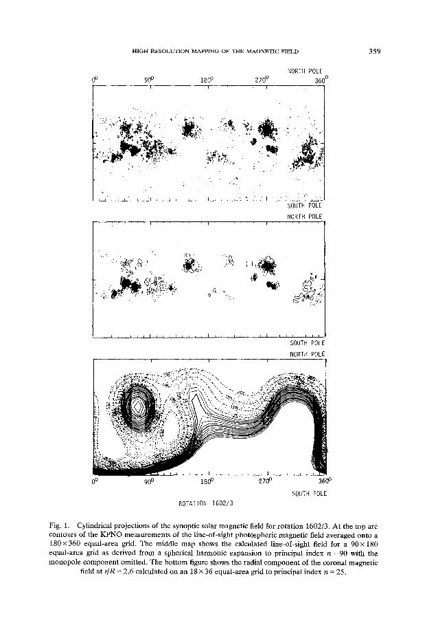
Fig. 1. Cylindrical projections of the synoptic solar magnet ic field for rotat ion 1602/3. A t the top are contours of the KPNO measurements of the l ine-of-sight photospher ic magnet ic field averaged onto a 1 8 0 x 3 6 0 equal-area grid. The middle map shows the calculated l ine-of-sight field for a 9 0 • equal -area grid as derived from a spherical harmonic expansion to principal index n = 90 with the monopole componen t omitted. The bo t tom figure shows the radial componen t of the coronal magnet ic

field at r/R = 2.6 calculated on an 18 x 36 equal-area grid to principal index n = 25.

360 M A R T I N D, A L T S C H U L E R E T AL.

6. Obtaining the Coefficients

To obtain the spherical harmonic coefficients, the 180 x 360 photospheric line-of- sight field values (Section 5) are read in from the magnetic tape and stored in large-core memory. Then for each value of the index m, the matrix A (Equation (20)) and the vector y (Equation (18)) are assembled and the resulting matrix equation (Equation (23)) is solved. The coefficients for all the different m are then stored on a second magnetic tape. The mathematical details are given in Section 3. Figure 1 shows synoptic maps (cylindrical projections) of the photospheric line- of-sight magnetic field. At the top are the KPNO averaged data values, in the middle are the values determined from 8280 spherical harmonic coefficients, with the monopole component omitted. Contours for both maps range from 350 to - 3 5 0 gauss. At the bottom is the radial field at 2.6 R.

7. Mapping the Coronal Magnetic Field

A zero-potential surface ensures the field lines are radial at some radius, usually chosen as Rw = 2.6R. This simple artifice provides a crude simulation of the effect of solar wind expansion on the coronal field. With the zero-potential surface, the magnetic field becomes (see also Altschuler and Newkirk, 1969; Equations (30) to (40))

Br(r, O, (9) = 2 U,(r)P~(O)(g'~ cos mq~ + h~ " sin m6), (37) r t = l r n = 0

Bo(r, O, 49) = - ~ Vn(r) (g~ cos mq5 + h~" sin mqS), (38) n = l m ~ 0

1 N d. B4,(r, 0, 4~) = s i - ~ n=~l m=o2. rnV,~(r)P'f(O)(g'2 sin m4~ - h~ cos rn4)), (39)

Un(r) = - R df~(r)/dr, V,~(r) = Rfn(r)/r. (40)

Once the coefficients g~, h , "~ are known, we can begin at any point in space (r, 0, 40 whether on the surface or at some convenient height, and trace the magnetic field line either radially inward or outward using Equations (37) through (40), a routine to generate associated Legendre polynomials and their derivatives, and a two-step Runge-Kutta procedure. (The four-step and two-step Runge- Kutta techniques provide maps which are indistinguishable.)

We have so far experimented with four basic kinds of maps: (1) Synoptic contour plots, for example of B,(r) at different values of radius r,

presented as cylindrical projections of a solar rotation. (2) 'Hairy-ball' global-scale maps showing coronal field lines which originate

from the photosphere. (3) 'Hairy-ball' global-scale maps which trace coronal field lines from an

equal-area grid at r = Rw back to the Sun's surface in order to locate the areas of the photosphere responsible for the radial open field lines.

H I G H ~ R E S O L U T I O N M A P P I N G O F T H E M A G N E T I C F I E L D 361

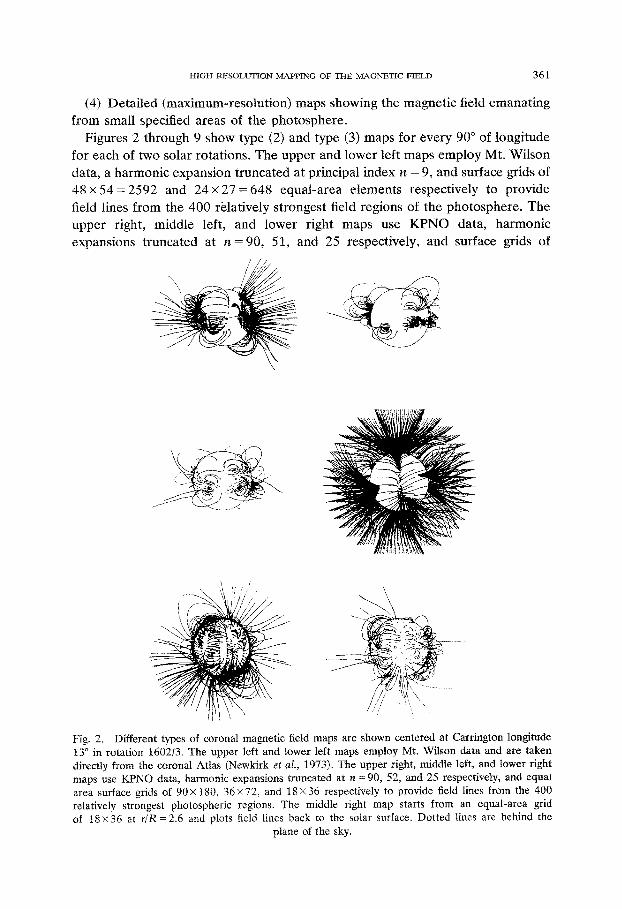
(4) D e t a i l e d ( m a x i m u m - r e s o l u t i o n ) m a p s showing the m a g n e t i c field e m a n a t i n g

f rom smal l speci f ied a reas of the p h o t o s p h e r e .

F igures 2 t h r o u g h 9 show type (2) and type (3) m a p s for eve ry 90 ~ of l ong i tude

for each of two so la r ro ta t ions . T h e u p p e r and l o w e r lef t m a p s e m p l o y Mt. W i l s o n

da ta , a h a r m o n i c e x p a n s i o n t r u n c a t e d at p r inc ipa l index n = 9, and sur face gr ids of

4 8 x 5 4 = 2 5 9 2 and 2 4 x 2 7 = 6 4 8 e q u a l - a r e a e l e m e n t s r e spec t ive ly to p rov ide

field l ines f rom the 400 r~la t ive ly s t ronges t f ield reg ions of the p h o t o s p h e r e . T h e

u p p e r r ight , m i d d l e left , and lower r igh t maps use K P N O da ta , h a r m o n i c

expans ions t r u n c a t e d at n = 9 0 , 51, and 25 respec t ive ly , a n d sur face grids of

/ / .

(

, , // ,

\ / i ~'�84 ,

Fig. 2. Different types of coronal magnetic field maps are shown centered at Carrington longitude 13 ~ in rotation 1602/3. The upper left and lower left maps employ Mt. Wilson data and are taken directly from the coronal Atlas ~ewkirk et al., 1973). The upper right, middle left, and lower right maps use KPNO data, harmonic expansions truncated at n = 90, 52, and 25 respectively, and equal area surface grids of 90• 180, 36/72, and 18 • 36 respectively to provide field lines from the 400 relatively strongest photospheric regions. The middle right map starts from an equal-area grid of 18• at r /R=2.6 and plots field lines back to the solar surface. Dotted lines are behind the

plane of the sky.

';"

\ )

O~

tO

Fig.

3.

Sam

e as

Fig

ure

2 bu

t fo

r ro

tati

on 1

604/

5.

L

%

~s::

~ �84

\

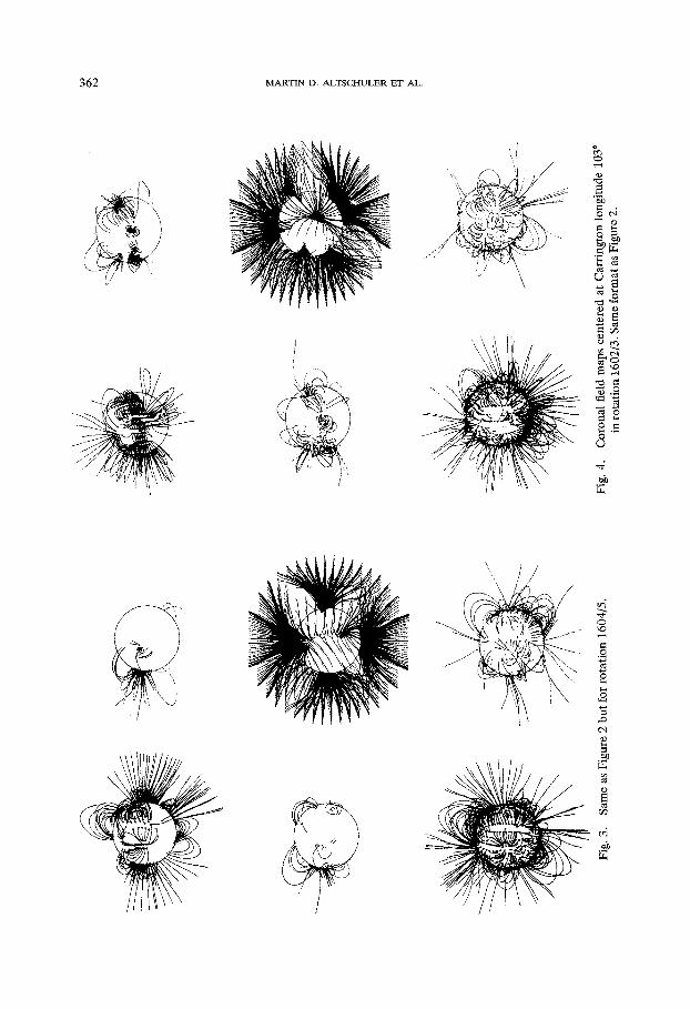
Fig.

4.

Cor

onal

fie

ld m

aps

cent

ered

at

Car

ring

ton

long

itud

e 10

3 ~

in r

otat

ion

1602

/3.

Sam

e fo

rmat

as

Figu

re 2

.

).

ccJ

..

�9 r

~�84

.~

-J

/

/J

/

r a#

:ig.

5.

Sam

e as

Fig

ure

4 bu

t fo

r ro

tati

on 1

604/

5.

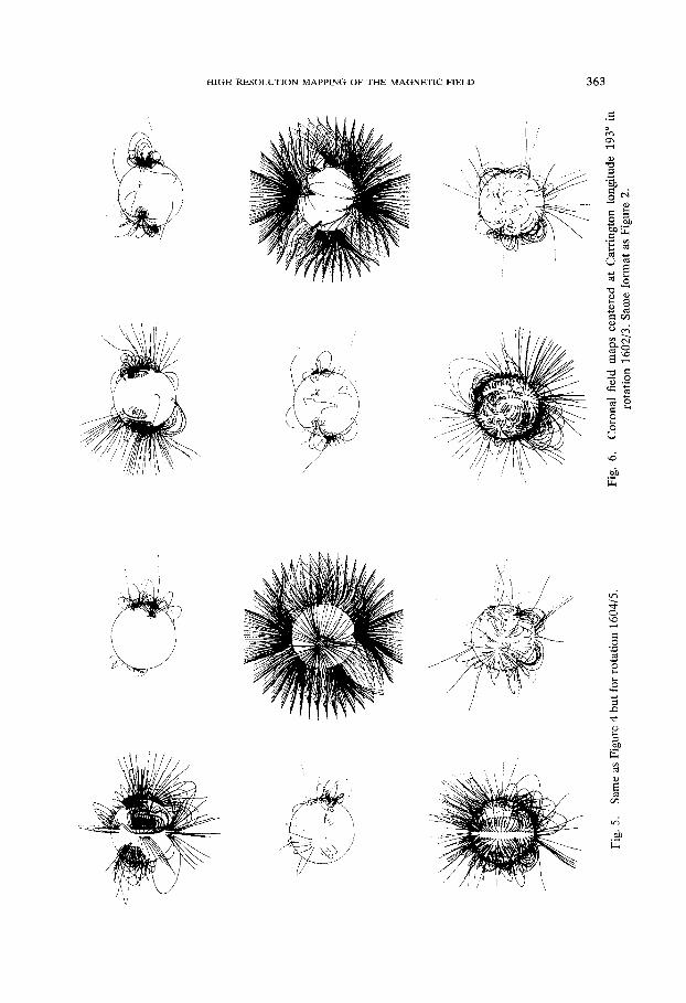
Fig.

6.

C

oron

al

fiel

d m

aps

cent

ered

at

Car

ring

ton

long

itud

e 19

3 ~

m

rota

tion

16

02/3

. Sa

me

form

at a

s F

igur

e 2.

/

. "

" D

, S

F''

/ )

\

~J

jJ

/ ,s

',

7ig.

7.

;am

e as

Fig

ure

6 b

ut

rota

tion

160

4/5.

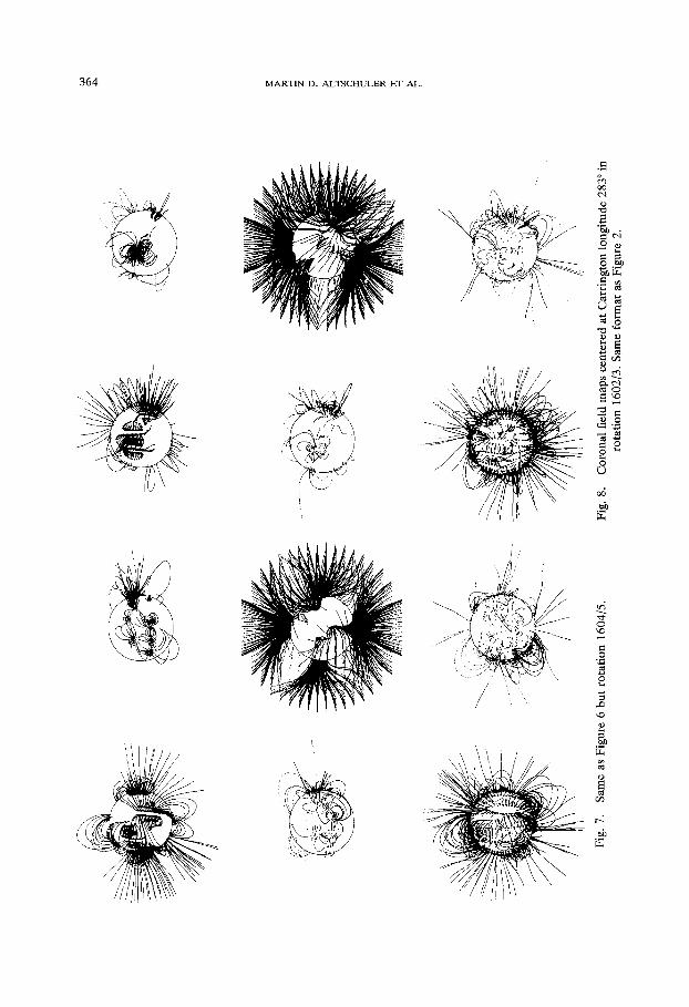
~i

g. 8

.

/Y

2oro

nal

fie

ld m

aps

cen

tere

d a

t C

arri

ngt

on lo

ngi

tud

e 28

30 i

n ro

tati

on 1

602/

3.

Sam

e fo

rmat

as

Fig

ure

2.


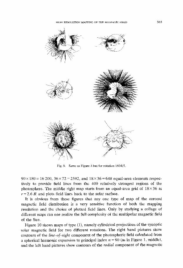
Fig. 9. Same as Figure 8 but for rotation 1604/5.

90 x 180 = 16 200, 36 x 72 = 2592, and 18 x 36 = 648 equal-area elements respectively to provide field lines from the 400 relatively strongest regions of the photosphere. The middle right map starts from an equal-area grid of 18 x 36 at r = 2.6 R and plots field lines back to the solar surface.

It is obvious from these figures that any one type of map of the coronal magnetic field distribution is a very sensitive function of both the mapping resolution and the choice of plotted field lines. Only by studying a collage of different maps can one realize the full complexity of the multipolar magnetic field

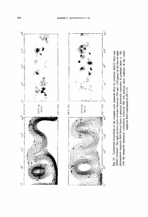
of the Sun. Figure 10 shows maps of type (I), namely cylindrical projections of the synoptic

solar magnetic field for two different rotations. The right hand pictures show contours of the line-of-sight component of the photospheric field calculated from a spherical harmonic expansion to principal index n = 90 (as in Figure 1, middle), and the left hand pictures show contours of the radial component of the magnetic

o 90

0 18

0 ~

's ,'.

:~!;2

: "~:

~,',;:,~

,"!';',

~ "~--

- :~:~

5~:_~

).' ",,

~'

,: .

,,., ~. ,

.,

fi ~

'~:,',:

,',::~

-:":~

:":"!~

!~:~

--:-~

~ i~

o o

oO

o 36

0 ~

270

360

900

180

270 o

N

OR

TH P

OLE

~

....

~

, ,

~

....

....

,

....

....

OTA

TIO

N

1602

/3

OU

TH P

OLE

JOR

TH P

OLE

OTA

TIO

N

1604

/5

io

90

~

1800

27

00

3600

SO

UTH

PO

LE

o ~o

~,

~

~ ',,~

,:.~:

.,:.:,~

.

.~.~

~.

~':,f

~,

,

i i

i ~

i i

d J

L I

i P

r L

t t

I t

i i

I i

i i

q i

I :

, ,

, ,

, ,

, I

o 90

0 18

0 o

270 o

36

00

7ig.

10.

C

ylin

dric

al p

roje

ctio

ns o

f th

e sy

nopt

ic s

olar

mag

neti

c fi

eld

for

rota

tion

s 16

02/3

(t

op)

and

604/

5 (b

otto

m).

The

rig

ht p

ictu

res

show

con

tour

s (b

etw

een

350

and

-350

gau

ss)

of t

he l

ine-

of-s

ight

~h

otos

pher

ic m

agne

tic

fiel

d de

rive

d fr

om a

sph

eric

al h

arm

onic

exp

ansi

on t

o pr

inci

pal

inde

x n

= 90

, vi

th t

he m

agne

tic

mon

opol

e co

mpo

nent

re

mov

ed.

The

le

ft p

ictu

res

show

con

tour

s of

the

ra

dial

m

agne

tic

fiel

d co

mpo

nent

at

#R =

2.6

.

H I G H R E S O L U T I O N M A P P I N G OF TI rE M A G N E T I C F I E L D 367

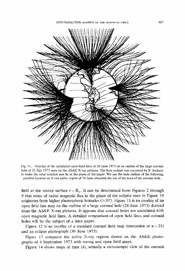
Fig. 11. Overlay of the calculated open-field lines of 28 June 1973 on an outline of the large coronal hole of 25 July 1973 seen on the AS&E X-ray pictures. The hole outline was corrected by B. Jackson to make the solar rotation axis lie in the plane of the paper. We use the hole outline of the following

rotation because an X-ray active region of 28 June obscured the toe of the boot of the coronal hole.

field at the source surface r = Rw. I t can be d e t e r m i n e d f rom Figures 2 t h rough

9 tha t some of rad ia l magne t i c flux in the p l ane of the ecl ipt ic seen in F igu re 10

or ig ina tes f rom h igher p h o t o s p h e r i c l a t i tudes (>30~ F igu re 11 is an ove r l ay of an

o p e n field l ine m a p on the ou t l ine of a l a rge co rona l ho le (28 June 1973) de r i ve d

f rom the A S & E X - r a y p ic tures . I t a p p e a r s tha t co rona l holes a re a s soc ia t ed with

o p e n m a g n e t i c field l ines. A d e t a i l e d c o m p a r i s o n of o p e n f ield l ines a n d co rona l

holes will be the sub jec t of a l a t e r p a p e r .

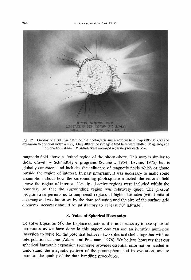
F igu re 12 is an o v e r l a y of a s t a n d a r d co rona l f ield m a p ( t runca t ion at n = 25)

and an ecl ipse p h o t o g r a p h (30 June 1973).

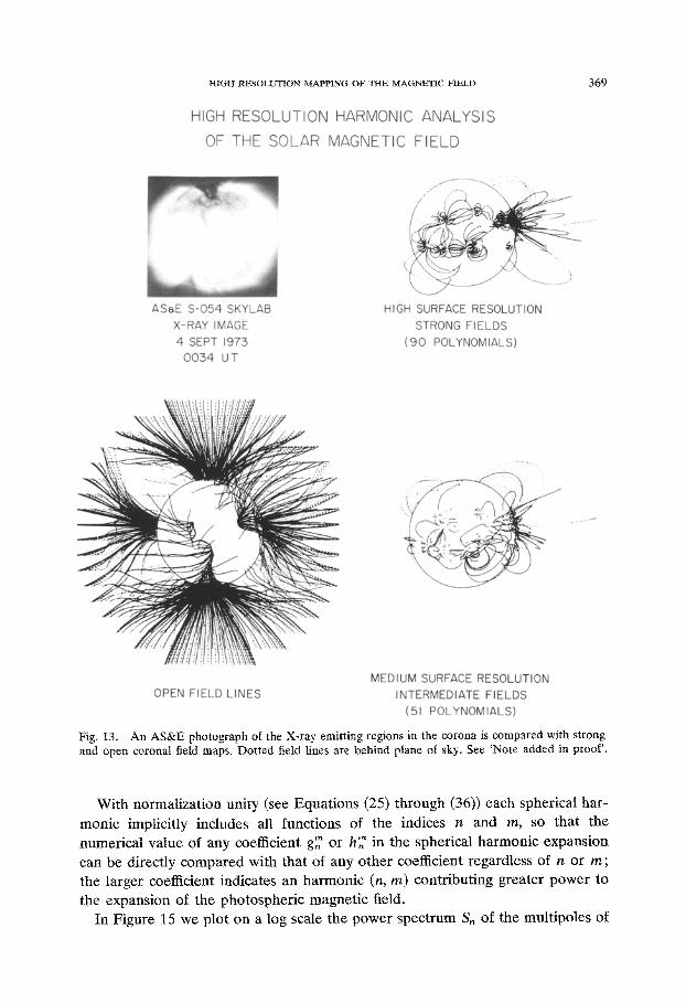
F igu re 13 c o m p a r e s the act ive X - r a y reg ions shown on the A S & E p h o t o -

g raphs of 4 S e p t e m b e r 1973 wi th s t rong and o p e n field maps .

F igure 14 shows maps of t ype (4), ac tua l ly a s t e r e osc op i c view of t he c o rona l

368 M A R T I N D. A L T S C H I J L E R E T AL.

Fig. 12. Overlay of a 30 June 1973 eclipse photograph and a coronal field map (18 x 36 grid and expansion to principal index n = 25). Only 400 of the strongest field lines were plotted. Magnetograph

observations above 70 ~ latitude were averaged separately for each pole.

magnetic field above a limited region of the photosphere. This map is similar to those drawn by Schmidt-type programs (Schmidt, 1964; Levine, 1975) but is

globally consistent and includes the influence of magnetic fields which originate outside the region of interest. In past programs, it was necessary to make some assumption about how the surrounding photosphere affected the coronal field above the region of interest. Usually all active regions were included within the boundary so that the surrounding region was relatively quiet. The present program also permits us to map small regions at higher latitudes (with limits of accuracy and resolution set by the data reduction and the size of the surface grid elements; accuracy should be satisfactory to at least 50 ~ latitude),

8. Value of Spherical Harmonics

To solve Equat ion (4), the Laplace equation, it is not necessary to use spherical harmonics as we have done in this paper; one can use an iterative numerical inversion to solve for the potential between two spherical shells together with an

interpolation scheme (Adams and Pneuman, 1976). We believe however that our spherical harmonic expansion technique provides essential information needed to understand the magnetic pat tern of the photosphere and its evolution, and to monitor the quality of the data handling procedures.

HIGH RESOLUT/ON MAPPING OF THE MAGNETIC ]03ELD 369

Fig. 13. An AS&E photograph of the X-ray emitting regions in the corona is compared with strong and open coronal field maps. Dotted field lines are behind plane of sky. See 'Note added in proof'.

With normalization unity (see Equations (25) through (36)) each spherical har-

monic implicitly includes all functions of the indices n and m, so that the numerical value of any coeff• g7 or h~ in the spherical harmonic expansion can be directly compared with that of any other coefficient regardless of n or m; the larger coefficient indicates an harmonic (n, m) contributing greater power to the expansion of the photospheric magnetic field.

In Figure 15 we plot on a log scale the power spectrum S, of the multipoles of

370 MARTIN D. ALTSCHULER ET AL.

;)

Fig. 14. Stereo views of the coronal magnetic field above a limited photospheric region.

the photospheric magnetic field. The multipolar spectrum is defined as

S~ = ~ [(g~)2+ (h~)2]. (41) ra

Thus the dipole contribution

S 1 = (g10)2-~ - ( g l ) 2 -[ - ( h l ) 2 , (42)

is the sum of three terms and the 2"-pole is the sum of 2n + 1 terms. Rotations 1602/1603 (15 June to 11 July 1973) and 1604/1605 (11 August to 7 September 1973) are shown on the left and right respectively in Figure 15.

Two conclusions can be drawn immediately. First, there is filtering of high spatial frequencies particularly for principal indices n -> 42. Second, the multipolar distribution of the photospheric magnetic field changed very little over two solar

rotations; this is especially striking for the lowest multipoles. Attenuat ion of high spatial frequencies is expected because the line-of-sight field

recorded for each bin of the synoptic grid is an average of many measurements over several days during which fine details are blurred by proper motion. The change in the power spectrum at n ~ 42 is consistent with a distribution of proper motion

velocities up to roughly 100 m s 1 and thus in good accord with direct observations of such velocities. We interpret the flattening of the power spectrum at n ~ 80 as due to the noise level of the instrument. Assuming that the noise spectrum is white, we determine the RMS noise level per synoptic grid element as about +0.3 gauss. This value is consistent with the noise level estimated on the basis of the noise in each original observation point and the total number of points which contribute to each synoptic grid element.

-i

10

~i

i

i +

il

+ i

i +I

i

+ i

i ll

lll

I i

i i

i'|"i

+

i +

I ~'

+ t

~ I

i i

t i Z

10 -2

10 -3

10 -4

,,

,,

i,

,,

+l

,,

,,

i,

+,

,l

++

+,

i,

,,

,i

,+

,+

i

....

! .

..

.

l~

to

20

30

4o

so

6o

;o

ao

90

10 -2

"iil

llil

illi

llil

lli+

llll

ilil

+lll

llil

t+il

(lll

10 -3

10 -4

-5L

0

10

20

30

40

50

60

70

80

90

�9

7'

0 0 rn

Fig.

15

. T

he p

ower

sp

ectr

um

S,,

vs n

of

the

m

ulti

pole

s of

the

pho

tosp

heri

c m

agne

tic

fiel

d fo

r ro

tati

ons

1602

/3 (

left

) an

d 16

04/5

(ri

ght)

. K

PN

O

data

wer

e us

ed.

The

ran

k-co

rrel

atio

n ag

reem

ent

(coe

ffic

ient

of

conc

orda

nce)

for

the

se p

ower

spe

ctra

is

96%

.

i0 -

I


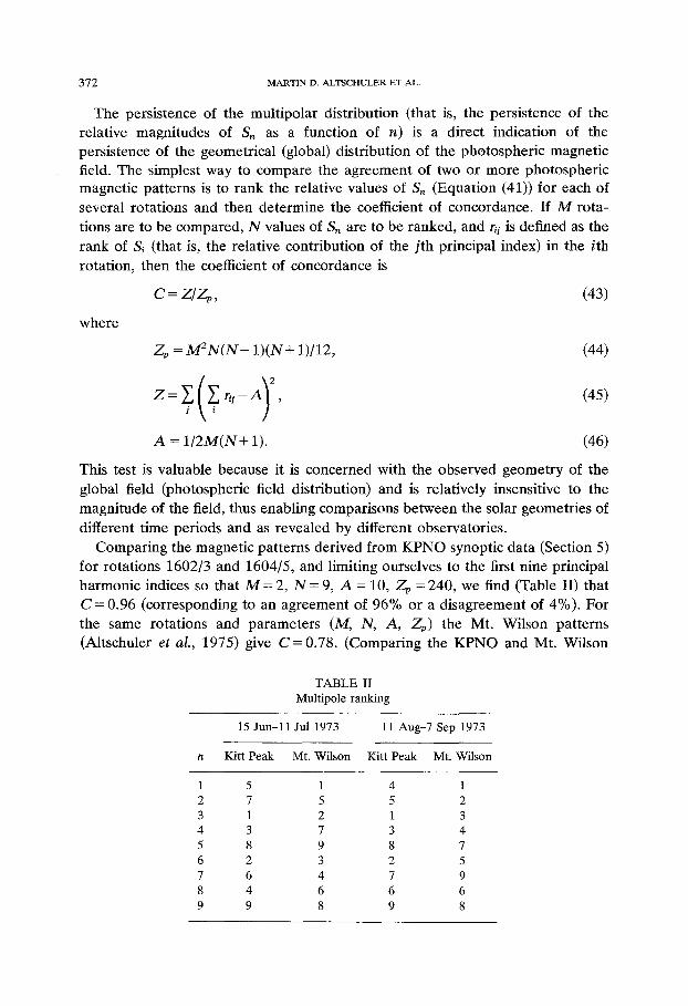
The persistence of the multipolar distribution (that is, the persistence of the relative magnitudes of Sn as a function of n) is a direct indication of the persistence of the geometrical (global) distribution of the photospheric magnetic field. The simplest way to compare the agreement of two or more photospheric magnetic patterns is to rank the relative values of Sn (Equation (41)) for each of

several rotations and then determine the coefficient of concordance. If M rota-

tions are to be compared, N values of Sn are to be ranked, and rij is defined as the

rank of Sj (that is, the relative contribution of the j th principal index) in the ith

rotation, then the coefficient of concordance is

where

C = Z / Z p , (43)

Zp = M a N ( N - 1) (N+ 1)/12, (44)

Z = ~ r l j - A , (45)

A = 1 / 2 M ( N + 1). (46)

This test is valuable because it is concerned with the observed geometry of the

global field (photospheric field distribution) and is relatively insensitive to the magnitude of the field, thus enabling comparisons between the solar geometr ies of

different t ime periods and as revealed by different observatories.

Compar ing the magnetic patterns derived from K P N O synoptic data (Section 5) for rotations 1602/3 and 1604/5, and limiting ourselves to the first nine principal

harmonic indices so that M = 2, N = 9, A = 10, Zp = 240, we find (Table II) that C = 0.96 (corresponding to an agreement of 96% or a disagreement of 4%). For the same rotations and parameters (M, N, A, Zp) the Mt. Wilson pat terns (Altschuler et al., 1975) give C = 0.78. (Comparing the K P N O and Mt. Wilson

TABLE II Multipole ranking

15 Jun-ll Jul 1973 11 Aug-7 Sep 1973

Kitt Peak Mt. Wilson Kitt Peak Mt. Wilson

1 5 1 4 1 2 7 5 5 2 3 1 2 1 3 4 3 7 3 4 5 8 9 8 7 6 2 3 2 5 7 6 4 7 9 8 4 6 6 6 9 9 8 9 8

H I G H R E S O L U T I O N M A P P I N G O F T H E M A G N E T I C F I E L D 373

patterns for those same periods, we find C=0.80 for rotation 1602/3 and C = 0.84 for rotation 1604/5.)

To determine the reason for the different degrees of persistence in the magnetic patterns derived from KPNO and Mt. Wilson data, we have sampled the concordance of the Mt. Wilson Sn values for consecutive solar rotations in quiet and active years. For quiet years the Mt. Wilson S, values have concordances which

average about 0.90. For active years, these concordances drop to about 0.60. Thus we suspect that our previous harmonic analysis of the Mt. Wilson data was affected by (1) the failure to measure accurately (without saturation) the higher field strengths (particularly the dynamic range from 100 to 1000 gauss) important within photospheric faculae and active regions, (2) the possible inaccuracy (or irreproducibility between consecutive rotations) of our statistical corrections for sunspot magnetic fields, and (3) the possible effects of averaging an entire active region into a single bin of the relatively coarse 30 • 36 synoptic grid. Because we have no KPNO data analyzed for consecutive rotations of active years, there is the possibility that strong and rapidly changing photospheric fields (that is, real events) had some effect on the global field pattern and hence on the Mt. Wilson concordances.

Our suspicions, however, are also supported by the particular values of the S, themselves. For rotations 1602/3 and 1604/5, the new method of analysis with KPNO data indicates that the octupole (n = 3) is the dominant multipole of the photospheric field, whereas the old method of analysis with the Mt. Wilson data indicates that the dipole (n = 1) is the dominant multipole. With Mt. Wilson data averaged to a 30 • 36 synoptic grid, our harmonic expansion to n = 9 should easily have detected an n = 3 octupole component. (Both Mt. Wilson and KPNO had good observational coverage in these periods). Comparing the corresponding coronal maps of these different analyses, we find that the various arcades and open field regions generally agree but that the Mt. Wilson maps show more open field lines. Considering both the distribution of active regions on the photosphere during these rotations and the concordances discussed above, we suspect that the octupole field is correct and that the photospheric fields greater than 100 gauss, which are not included in the Mt. Wilson data, provide significant contributions to the global photospheric and coronal field patterns. Our statistical correction for sunspot fields applied to the Mt. Wilson data does not treat the flux of the strong non-sunspot fields from extended active areas of the photosphere.

Thus the improved dynamic range of the KPNO magnetograph data should allow more accurate determination of the coefficients of the harmonic expansion of the photospheric magnetic field, particularly during active years. Consequently, any changes in the coefficients derived from the KPNO data should be a more trustworthy indication of real changes in the photospheric field pattern.

Finally it should be noted from (1) the flatness of the power spectrum of S, to at least principal index n =42 (Figure 15) and (2) the r -("+1) dependence of the magnetic field on principal index (Equation (6) and Equations (37) through (40)) that


the electric currents which produce the observed photospheric magnetic field must have a significant shallow component, ff R' is the largest radius at which an electric current occurs and R is the solar radius (where R ' < R ) , theni the ratio ( R ' / R ) 43 drops to 1% of its value at a depth R - R ' . ~ 7 0 Mm. We plan to run a case without averaging the data over several days to see whether S, vs n remains flat much beyond n = 42.

9. Conclusions

We have improved both the mapping of the current-free magnetic field of the solar corona and the reliability of the spherical harmonic analysis of the photospheric magnetic field pattern by using (1) data with much greater dynamical range and spatial resolution than previously available, and (2) a new computer algorithm which permits spherical harmonic expansion to a much higher value of the principal index. Coronal field maps can be drawn for local regions, for just the open field lines, and for various spatial resolutions on a global scale. An understanding of the complex coronal magnetic field pattern requires a careful study of several different kinds of coronal map, each of which provides different information.

The Sun's magnetic field pattern is complex and dynamic. The evolving photospheric field alters the coronal magnetic field pattern and thereby the magnetic environment of our own planet. With the techniques described in this paper, magnetographs capable of high spatial resolution over a large dynamical range can be used to monitor (in real time if necessary) the changing large-scale magnetic patterns of the photosphere and corona as assiduously as we now monitor the global weather patterns of the Earth.

Acknowledgements

We thank E. Hildner, B. Jackson, A. P. Miedaner, D. E. Trotter, and D. Wilson for their invaluable assistance and encouragement, R. Hansen and S. Hansen for their unceasing criticisms of potential field methods during these past years, and R. Howard for reviewing the manuscript and many helpful comments. Some of this work was done under the auspices of the Skylab Workshop. The work of one of us (RHL) was supported by NASA contract NA 5-3949.

Note added in proof: In Figure 13, the words '90 polynomials' and '51 polynomials' should be interpreted as max(n)= 90 and max(n)= 51, respectively.

References

Adams, J. and Pneuman, G. W.: 1976, Solar Phys., 46, 185. Altschuler, M. D. and Newkirk, G. Jr.: 1969, Solar Phys. 9, 131. Altschuler, M. D., Trotter, D. E., Newkirk, G. Jr., and Howard, R.: 1975, Solar Phys. 41, 225.

H I G H R E S O L U T I O N M A P P I N G OF T H E M A G N E T I C F IELD 375

Chapman, S. and Bartels, J.: 1940, Geomagnetism, Oxford Univ. Press. Dulk, G. A., Altschuler, M. D., and Smerd, S. F.: 1971, Astrophys. Letters 8, 235. Harvey, J. W.: 1969, Ph.D. thesis, University of Colorado. Levine, R. H.: 1975, Solar Phys. 44, 365. Livingston, W. and Harvey, J.: 1971, in R. Howard (ed.), 'Solar Magnetic Fields', IAU Syrup. 43, 616. Livingston, W. C., Harvey, J., Slaughter, C., and Trumbo, D.: 1976, Applied Optics 15, 40. Nakagawa, Y.: 1973, Astron. Astrophys. 27, 95. Newkirk, G. Jr.: 1971, in C. J. Macris (ed.), Physics of the Solar Corona, D. Reidel Publ., Dordrecht,

p. 66. Newkirk G. Jr. and Altschuler, M. D.: 1970, Solar Phys. 13, 131. Newkirk, G. Jr., Trotter, D. E., Altschuler, M. D., and Howard, R.: 1973, A Microfilm Atlas of

Magnetic Fields in the Solar Corona, NCAR-TN/STR-85. Rust, D. M. and Roy, J. R.: 1971, in R. Howard (ed.), ~Solar Magnetic Fields', IAU Syrup. 43, 569. Schatten, K. H.: 1971a, Cosmic Electrodynamics 2, 232. Schatten, K. H.: 1971b, in R. Howard (ed.), 'Solar Magnetic Fields', IAU Syrup. 43, 595. Schatten, K. H., Wilcox, J. M., and Ness, N. F.: 1969, Solar Phys. 6, 442. Schmidt, A.: 1895, Abhandl. Bayer Akad. Wiss. Miinchen II. Klasse 19, 1. Schmidt, H. U.: 1964, in AAS-NASA Syrup. on the Physics of Solar Flares, NASA SP-50, p. 107. Smerd, S. F. and Dulk, G. A.: 1971, in R. Howard (ed.), 'Solar Magnetic Fields', [AU Syrup. 43, 616. Uchida, Y. Altschuler, M. D., and Newkirk, G. Jr.: 1973, Solar Phys. 28, 495.

high resolution mapping of the magnetic field of the solar corona

Documents