HIGH PERFORMANCE EXACT LINEAR ALGEBRA

by

Bryan Youse

A dissertation submitted to the Faculty of the University of Delaware in partialfulfillment of the requirements for the degree of Doctor of Philosophy in Computer &Information Sciences

Spring 2015

c© 2015 Bryan YouseAll Rights Reserved

HIGH PERFORMANCE EXACT LINEAR ALGEBRA

by

Bryan Youse

Approved:Errol Lloyd, Ph.D.Chair of the Department of Computer & Information Sciences

Approved:Babatunde A. Ogunnaike, Ph.D.Dean of the College of Engineering

Approved:James G. Richards, Ph.D.Vice Provost for Graduate and Professional Education

I certify that I have read this dissertation and that in my opinion it meets theacademic and professional standard required by the University as a dissertationfor the degree of Doctor of Philosophy.

Signed:B. David Saunders, Ph.D.Professor in charge of dissertation

I certify that I have read this dissertation and that in my opinion it meets theacademic and professional standard required by the University as a dissertationfor the degree of Doctor of Philosophy.

Signed:Jeremy Johnson, Ph.D.Member of dissertation committee

I certify that I have read this dissertation and that in my opinion it meets theacademic and professional standard required by the University as a dissertationfor the degree of Doctor of Philosophy.

Signed:Michela Taufer, Ph.D.Member of dissertation committee

I certify that I have read this dissertation and that in my opinion it meets theacademic and professional standard required by the University as a dissertationfor the degree of Doctor of Philosophy.

Signed:John Cavazos, Ph.D.Member of dissertation committee

I certify that I have read this dissertation and that in my opinion it meets theacademic and professional standard required by the University as a dissertationfor the degree of Doctor of Philosophy.

Signed:David Wood, Ph.D.Member of dissertation committee

ACKNOWLEDGEMENTS

I would like to deeply thank all of those friends and family who believed in mefrom the beginning. I simply could not have proceeded without your support. Specialthanks are owed to:

• My parents, for the various opportunities for growth they provided me throughoutmy life, by virtue of their own hard work.

• My grandfather, who had been calling me “doctor” long before it was clear thatI would complete this work.

• My advisor, Dave, who devoted countless hours in aiding my journey. His enthu-siasm for the subject matter was contagious. I will forever fondly recall the lateevenings of pair-programming in the various labs that our somewhat nomadicgroup occupied at one time or another. I view this time spent as collaborationof not mere colleagues, but friends.

• Finally my wife, Leah, earns my deepest gratitude. She unflinchingly encouraged,reassured, and cared for me at all times, but most especially when I needed it.

I love you.

v

TABLE OF CONTENTS

LIST OF TABLES . . . . . . . . . . . . . . . . . . . . . . . . . . . . . . . . ixLIST OF FIGURES . . . . . . . . . . . . . . . . . . . . . . . . . . . . . . . xLIST OF ALGORITHMS . . . . . . . . . . . . . . . . . . . . . . . . . . . xiLIST OF SYMBOLS . . . . . . . . . . . . . . . . . . . . . . . . . . . . . . xiiABSTRACT . . . . . . . . . . . . . . . . . . . . . . . . . . . . . . . . . . . xiii

Chapter

1 INTRODUCTION . . . . . . . . . . . . . . . . . . . . . . . . . . . . . . 1

2 FINITE FIELD DATA COMPRESSION . . . . . . . . . . . . . . . . 4

2.1 Introduction . . . . . . . . . . . . . . . . . . . . . . . . . . . . . . . . 4

2.1.1 Prior work . . . . . . . . . . . . . . . . . . . . . . . . . . . . . 5

2.2 Bit-packing . . . . . . . . . . . . . . . . . . . . . . . . . . . . . . . . 5

2.2.1 Faster bit-packing . . . . . . . . . . . . . . . . . . . . . . . . . 122.2.2 Extending to other prime fields . . . . . . . . . . . . . . . . . 14

2.3 Bit-slicing . . . . . . . . . . . . . . . . . . . . . . . . . . . . . . . . . 19

2.3.1 Specialized arithmetic . . . . . . . . . . . . . . . . . . . . . . 22

2.4 Summary . . . . . . . . . . . . . . . . . . . . . . . . . . . . . . . . . 25

vi

3 STRONGLY REGULAR GRAPH 3-RANKS . . . . . . . . . . . . . 27

3.1 Introduction . . . . . . . . . . . . . . . . . . . . . . . . . . . . . . . . 27

3.1.1 Prior work . . . . . . . . . . . . . . . . . . . . . . . . . . . . . 28

3.2 Obtaining rank(D(3, 7)) . . . . . . . . . . . . . . . . . . . . . . . . . 29

3.2.1 Space and time efficient p-Rank . . . . . . . . . . . . . . . . . 303.2.2 Certified 3-Rank . . . . . . . . . . . . . . . . . . . . . . . . . 40

3.3 Obtaining rank(D(3, 8)) . . . . . . . . . . . . . . . . . . . . . . . . . 44

3.3.1 Motivation . . . . . . . . . . . . . . . . . . . . . . . . . . . . . 443.3.2 Size & scope . . . . . . . . . . . . . . . . . . . . . . . . . . . . 453.3.3 Producer/consumer: A first try . . . . . . . . . . . . . . . . . 46

3.3.3.1 Broad implementation . . . . . . . . . . . . . . . . . 483.3.3.2 The building blocks . . . . . . . . . . . . . . . . . . 583.3.3.3 A failure . . . . . . . . . . . . . . . . . . . . . . . . . 62

3.3.4 Producer/consumer: cut out the middle-man . . . . . . . . . . 64

3.3.4.1 Revised big-picture layout . . . . . . . . . . . . . . . 653.3.4.2 Revised building blocks . . . . . . . . . . . . . . . . 683.3.4.3 Shared-memory parallelism . . . . . . . . . . . . . . 70

3.3.5 Obtaining rank(M) . . . . . . . . . . . . . . . . . . . . . . . . 723.3.6 A final barrier . . . . . . . . . . . . . . . . . . . . . . . . . . . 74

3.3.6.1 The panacea . . . . . . . . . . . . . . . . . . . . . . 75

3.3.7 Further applications . . . . . . . . . . . . . . . . . . . . . . . 77

3.4 Summary . . . . . . . . . . . . . . . . . . . . . . . . . . . . . . . . . 78

vii

4 EXACT RATIONAL LINEAR SYSTEM SOLVER . . . . . . . . . 80

4.1 Introduction . . . . . . . . . . . . . . . . . . . . . . . . . . . . . . . . 80

4.1.1 Relation to prior work . . . . . . . . . . . . . . . . . . . . . . 80

4.2 Background . . . . . . . . . . . . . . . . . . . . . . . . . . . . . . . . 834.3 Confirmed continuation and output sensitivity . . . . . . . . . . . . . 86

4.3.1 An adaptive approach . . . . . . . . . . . . . . . . . . . . . . 864.3.2 Overflowing doubles . . . . . . . . . . . . . . . . . . . . . . . 884.3.3 Early termination . . . . . . . . . . . . . . . . . . . . . . . . . 89

4.4 Dyadic rational to rational reconstruction . . . . . . . . . . . . . . . . 904.5 Experiments . . . . . . . . . . . . . . . . . . . . . . . . . . . . . . . . 954.6 Summary . . . . . . . . . . . . . . . . . . . . . . . . . . . . . . . . . 102

5 SUMMARY . . . . . . . . . . . . . . . . . . . . . . . . . . . . . . . . . . 103

5.1 Future Work . . . . . . . . . . . . . . . . . . . . . . . . . . . . . . . . 105

BIBLIOGRAPHY . . . . . . . . . . . . . . . . . . . . . . . . . . . . . . . . 106

Appendix

A REMOTE OBJECTS WITH PYRO . . . . . . . . . . . . . . . . . . 111B F3 BIT-SLICING “STEPPER” . . . . . . . . . . . . . . . . . . . . . . 113

B.1 File-stepper . . . . . . . . . . . . . . . . . . . . . . . . . . . . . . . . 115

viii

LIST OF TABLES

2.1 Best bit-packing for small prime fields of interest. . . . . . . . . . . 10

2.2 Semi-normalized bit-packing performance improvements. . . . . . . 18

2.3 Speed of vector operations over F3. . . . . . . . . . . . . . . . . . . 26

3.1 Running time for computing the ranks of Dickson adjacency matrices,with summation and certificate. . . . . . . . . . . . . . . . . . . . . 44

3.2 Running time for computing the ranks of Dickson adjacency matrices:fully parallelized implementation. . . . . . . . . . . . . . . . . . . . 75

3.3 Known ranks for adjacency matrices of certain strongly regular graphfamilies. . . . . . . . . . . . . . . . . . . . . . . . . . . . . . . . . . 79

4.1 Examples of numeric failure to converge. . . . . . . . . . . . . . . . 96

4.2 Dixon, Wan, and Overlap algorithm performance comparison. . . . 101

ix

LIST OF FIGURES

2.1 A closeup of a machine word utilizing bit-packing, and a view of thesavings bit-packing affords. . . . . . . . . . . . . . . . . . . . . . . 7

2.2 Performance and space gains using vanilla bit-packing for small primefields. . . . . . . . . . . . . . . . . . . . . . . . . . . . . . . . . . . 11

2.3 Flowchart depicting the four bit-operations needed forsemi-normalization for bit-packed F3. . . . . . . . . . . . . . . . . . 13

2.4 A repetition of Figure 2.2(c) including semi-normalization data . . 17

2.5 The flow of a series of SN3 operations. . . . . . . . . . . . . . . . . 19

2.6 A closeup of two machine words utilizing bit-slicing to store F3

values, and a view of savings bit-slicing affords. . . . . . . . . . . . 20

2.7 Figure 2.2(a) updated with data points for semi-normalizedbit-packing and bit-slicing. . . . . . . . . . . . . . . . . . . . . . . . 24

3.1 Butterfly construction for b = 8. . . . . . . . . . . . . . . . . . . . . 32

3.2 Decomposition and compression of the matrix A. . . . . . . . . . . 50

3.3 Filesystem activity during parallel build of D(3, 8). . . . . . . . . . 63

3.4 A contrast of Figure 3.3 with the real time file-system activity of therevised parallel decomposition. . . . . . . . . . . . . . . . . . . . . 68

3.5 Multithreaded parallel scalability for the routine of building a columnblock. . . . . . . . . . . . . . . . . . . . . . . . . . . . . . . . . . . 73

4.1 Dense and sparse system performance comparison between theOverlap method and Dixon’s method. . . . . . . . . . . . . . . . . . 100

x

LIST OF ALGORITHMS

1 Marshalling finite field element data to enable bit-packing. . . . . . 6

2 Extracting finite field element data from a bit-packed representation. 8

3 Converting semi-normalized values to F3 representation. . . . . . . 14

4 General semi-normalization for bitpacking Mersenne-prime fields. . 16

5 Bit-slice a finite field element. . . . . . . . . . . . . . . . . . . . . . 21

6 Extracting finite field element data from a bit-sliced representation. 22

7 F3 addition with bit-slicing. . . . . . . . . . . . . . . . . . . . . . . 23

8 F3 negation/multiplication by two. . . . . . . . . . . . . . . . . . . 23

9 Confirmed continuation iterative refinement to solve Ax = b. . . . . 87

10 Confirmed continuation iterative refinement with Early Terminationto solve Ax = b. . . . . . . . . . . . . . . . . . . . . . . . . . . . . . 89

11 Vector conversion from dyadic to rational. . . . . . . . . . . . . . . 94

xi

LIST OF SYMBOLS

| Bitwise-OR.

& Bitwise-AND.

⊕ Bitwise-XOR.

∼ Bitwise-NOT.

� Bitshift left.

� Bitshift right.

++ Increment operator.

% Modulus operator.

b c Integer floor.

d e Integer ceiling.

‖A‖ Matrix norm.

‖A‖∞ Infinity norm.

xii

ABSTRACT

This is a study in exact computational linear algebra consisting of two parts.

First the problem of computing the p-rank of an integer matrix with particular emphasis

on the case when the matrix is large and dense, the rank is relatively small, and the

prime is tiny (such as p = 3). Second is a numeric-symbolic rational linear system

solver using an iterative refinement approach.

The rank problem arises from the study of difference sets of finite groups and

their corresponding strongly regular graphs. The ranks of the adjacency matrices

representing these graphs are sought. These matrices, defined in sequences, grow too

large for previously known rank algorithms. Prior solutions either require too much

memory or are too computationally costly for the scenario of a large matrix with

much lower rank. The expected low rank invites us to find a space- and time-efficient

algorithm for this special case. The heuristic methods detailed here form a Monte Carlo

algorithm which is essentially optimal when the rank is sufficiently small. Several tools

are used in concert with the new algorithm which are vital in computing the rank of

some of the larger matrices of the sequences, which contain on the order of peta-entries.

A suite of finite-field data compression tools is discussed. Additionally, a framework

for distributed- and shared-memory parallelism is detailed.

The rational linear system solver produces, for each entry of the solution vector,

a rational approximation with denominator a power of two. From this representation,

the correct rational entry can be reconstructed. Our method is a numeric-symbolic

hybrid in that it uses an approximate numeric solver at each iteration together with a

symbolic (exact arithmetic) residual computation and symbolic rational reconstruction.

It is able to be output sensitive (i.e. terminate early) with provably correct result.

Alternatively, the algorithm may be used without the rational reconstruction to obtain

xiii

an extended precision floating point approximation of any specified precision. The chief

contributions of the method and implementation are confirmed continuation, highly

tuned rational reconstruction, and fast, robust performance.

All work contained herein contributes to the LinBox library for exact linear

algebra.

xiv

Chapter 1

INTRODUCTION

The purpose of this study is to explore and synthesize methods to increase the ef-

ficiency of selected exact linear algebra problems. Traditional numerical approximation

methods, prevalent in scientific and engineering computing today, provide solutions at

best accurate to the level of the precision of the machines on which they run. This ap-

proach is nevertheless popular due to generally fast computations and the approximate

nature of some input data. Symbolic techniques, those used to solve linear algebra prob-

lems exactly, offer the significant feature of providing answers completely free of error.

This benefit often comes at the cost of additional computational resources than anal-

ogous numerical methods would employ. Still, there exists healthy demand for exact

results; many applications stand to benefit from exact computation even if the nature

of the input data is approximate. Thanks to advances in computing hardware, namely

cheaper, vaster memory and faster, more numerous processors, exact computations are

in the realm of practical possibility for many problems. This growing complexity in the

computing landscape offers many avenues for improving algorithmic performance. Tai-

loring algorithms to diverse architectures, cache sizes, hardware arithmetic methods,

and parallel computation models is necessary to achieve peak performance. The work

in this thesis takes advantage of these strategies to improve efficiency of algorithms

found in the software library LinBox [1].

LinBox is a high performance, exact linear algebra C++ template library that

provides solutions for problems over arbitrary precision integers, rational numbers, and

1

finite fields. Particular problems include matrix rank, determinant, minimal polyno-

mial, characteristic polynomial, linear system solving, and Smith normal form. Solu-

tions exist for general dense matrices as well as sparse matrices, those matrices popu-

lated primarily with zeroes. Many specializations are offered for both dense and sparse

matrix variants that are specifically structured so that certain characteristics can be

algorithmically exploited.

An important area to the realm of exact computation is that of finite field arith-

metic. In Chapter 2 we will discuss various ways to improve arithmetic over small prime

finite fields. Special forms of compression have been developed to the end of lowering

both algorithm running time and memory footprint. Here we describe two known com-

pression schemes that greatly benefit computing with small prime fields, here called

bit-packing and bit-slicing. We provide an implementation of the compression methods

in LinBox, and detail our key innovations to the schemes. We demonstrate the value

of our specializations with experimental data.

The specific innovations will be illustrated by their inclusion in a solution to the

exact rank computation investigated in Chapter 3. In this chapter, the ranks we are

searching for are conjectured to be considerably smaller than the size of the matrices

on which we compute. We provide a novel, Monte Carlo algorithm tailor-made for such

a scenario, one wherein previously existing algorithms for computing rank prove either

too time-consuming, too memory-hungry, or both. In fact we compute with matrices

so large that shared and distributed parallelism is a necessity. We develop and outline

a multi-tiered parallel solution to computing the ranks of matrices peta-scale in storage

requirement. We explore and learn from some of the failures encountered along the

way. This completed work shows large performance gains over the previous state of

the art, and has achieved results that encourage pushing the algorithm to ever-larger

problems.

Chapter 4 discusses an entirely new topic under the wide umbrella of exact

computational algebra, that of rational linear system solving. In this chapter we employ

2

the aforementioned approximate numeric arithmetic within the confines of an exact-

answer algorithm in a hybrid solution known as a numeric-symbolic method. The idea

behind the marriage of numeric and symbolic computing is to exploit the gigaFLOPS

of power found in current floating-point units while still producing exact results. This

can prove advantageous over either using software extensions for representing large

integers, or resorting to finite field methods, two common symbolic techniques. We

offer a novel method of detecting overlap between successive numeric computations,

which we call the confirmed-continuation method. This key improvement helps a pre-

existing algorithm achieve improved performance and increased stability for solving

rational linear systems, a key solution offered by LinBox.

3

Chapter 2

FINITE FIELD DATA COMPRESSION

2.1 Introduction

Let Fp denote the finite field of size p. The field elements are 0 . . . p − 1 with

arithmetic modulo the prime p. Small finite field elements can be represented by many

fewer bits than are in a typical machine word. In this chapter let r be the number

of bits required to represent each element in a field. Fp elements require r = dlog2 pe

bits to fully represent. For instance F5 requires r = 3, e.g. 0 = 0002, 1 = 0012, 2 =

0102, 3 = 0112, 4 = 1002.

“Machine word” refers to the fixed-size number of bits that a given computer

architecture uses as its computational unit. In this chapter let l be the bit-length of a

machine word. Modern general purpose computers commonly have l = 32 or 64 bits.

Thus special compression for in-memory storage of small finite-field elements can be

used, appreciably decreasing both data-storage space requirements and common kernel

running times. The space-efficiency is of course an inherent property of our data com-

pression, while the running time efficiency follows from being able to perform arithmetic

operations on multiple elements simultaneously. This scheme is a form of Single In-

struction, Multiple Data (SIMD) Parallelism as defined in Flynn’s taxonomy of parallel

architectures [2]. Typically, the SIMD designation would refer to an architecture specif-

ically designed for performing instructions on multiple words simultaneously. While

of course our methodology does not preclude the use of such SIMD-capable hardware,

it achieves the end of the SIMD-parallelism model from within basic machine words.

In other words, though specialized hardware would certainly still prove beneficial, the

benefits of our improved data representation can be seen on general-purpose hardware

4

as well. Specifically, we employ variations on two compression schemes, bit-packing

and bit-slicing, each with different strengths and weaknesses.

Before these schemes can be illustrated in depth, first we must establish a lan-

guage for discussing finite-field compression. First let fx represent the space-efficiency

factor of a compression scheme, x, over the naive storage method of word-per-element.

The values of x used will be b for “basic bit-packing”, p for “bit-packing” and s for

“bit-slicing”. That is, fx describes the number of field elements representable with a

single machine word, since the elements-per-word in the naive scheme is always 1.

2.1.1 Prior work

Modern high-level languages and machinery replete with memory have both

served to limit the need to resort to bit-fiddling. But the concept of storing separate but

related values within singular inherent types has been well-explored. An early instance

of packing single bits into larger inherent types is the implementation of “bit-fields”

in the C Programming Language [3]. Later the C++ Standard Template Library [4]

would extend this concept to store arbitrary-length bit vectors with its “bitset” object.

Although these examples are primarily aimed at saving storage space, programmers

have exploited the SIMD nature of computing with word-compressed data. Boothby

and Bradshaw [5] detail some history with classical bit-packing methods, and introduce

the concept and key features of bit-slicing for small prime fields. Albrecht, Bard, and

Hart [6] have implemented bit-packing/bit-slicing for F2 in the M4RI software [7].

The combination of their thorough exposition and optimized implementation has been

highly influential on our development of the F3 compression technologies detailed here.

2.2 Bit-packing

Bit-packing involves marshalling field elements to fit alongside one another

within a single machine word. Using the defined values l and r from Section 2.1,

we can immediately calculate the basic bit-packing factor, fb = b lrc. If data storage

5

were the only concern, this would be sufficient, but almost always we desire to per-

form arithmetic operations on the compressed data. We must account for potential

bit-overflow during, say, addition or multiplication. Therefore we allocate a bit buffer

to catch this bit-overflow and let b refer to its bit-length. For general bit-packing, b is

adjustable and negotiable to best serve a given application’s needs. Thus, r+b denotes

the number of bits available to store each packed field element. Then the bit-packing

factor is fp = b lr + b

c. For instance, consider packing F3 values into sixty-four bit

words and allocating a single bit for carries, i.e. b = 1. Using the formula above,

r = 2 for F3. So the compression factor fp = b 642 + 1c = 21. The preceding can be

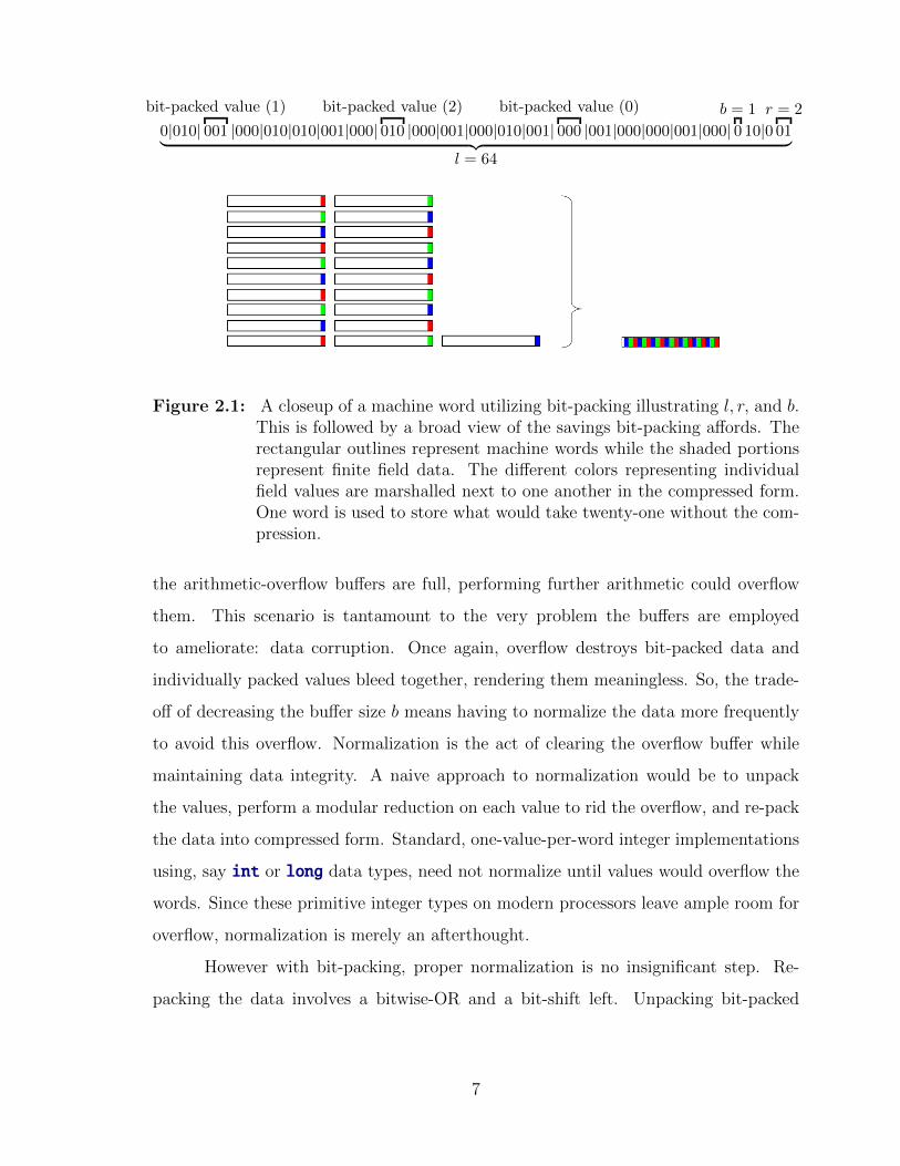
visualized with the aid of Figure 2.1, including the role of values l, r, and b.

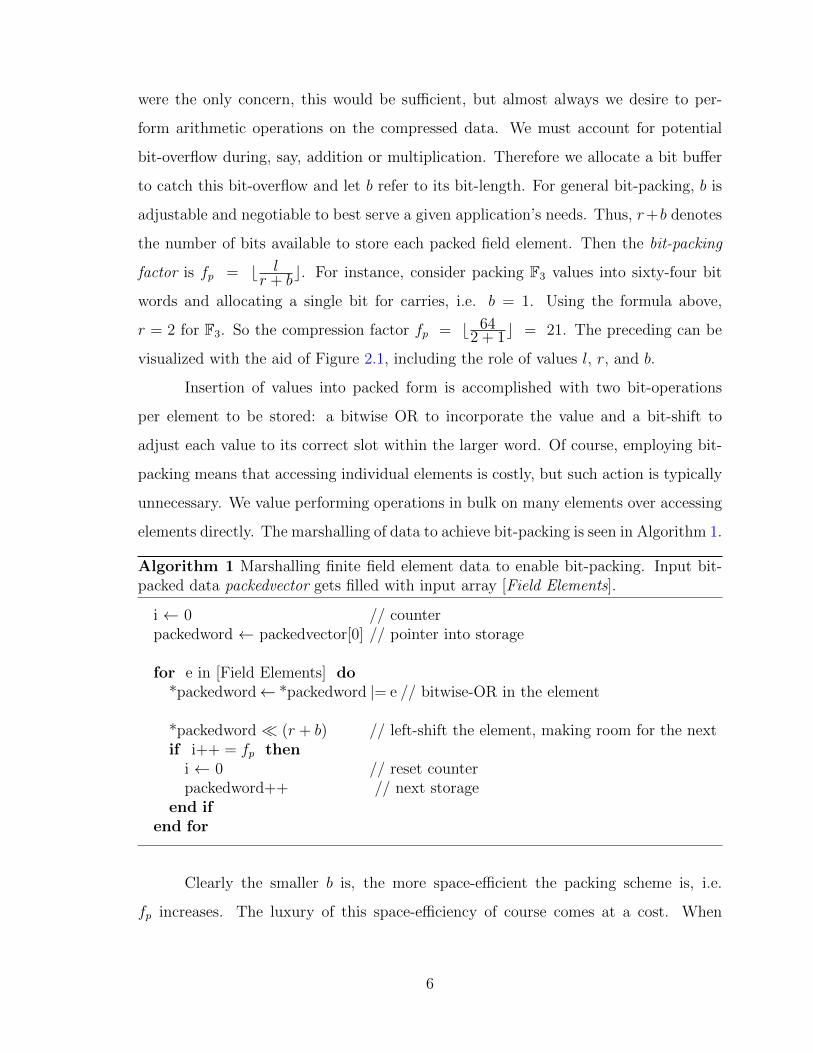
Insertion of values into packed form is accomplished with two bit-operations

per element to be stored: a bitwise OR to incorporate the value and a bit-shift to

adjust each value to its correct slot within the larger word. Of course, employing bit-

packing means that accessing individual elements is costly, but such action is typically

unnecessary. We value performing operations in bulk on many elements over accessing

elements directly. The marshalling of data to achieve bit-packing is seen in Algorithm 1.

Algorithm 1 Marshalling finite field element data to enable bit-packing. Input bit-packed data packedvector gets filled with input array [Field Elements].

i ← 0 // counterpackedword ← packedvector[0] // pointer into storage

for e in [Field Elements] do*packedword← *packedword |= e // bitwise-OR in the element

*packedword � (r + b) // left-shift the element, making room for the nextif i++ = fp then

i ← 0 // reset counterpackedword++ // next storage

end ifend for

Clearly the smaller b is, the more space-efficient the packing scheme is, i.e.

fp increases. The luxury of this space-efficiency of course comes at a cost. When

6

0|010|bit-packed value (1)

001 |000|010|010|001|000|bit-packed value (2)

010 |000|001|000|010|001|bit-packed value (0)

000 |001|000|000|001|000|b = 1

0 10|0r = 2

01︸ ︷︷ ︸l = 64

Figure 2.1: A closeup of a machine word utilizing bit-packing illustrating l, r, and b.This is followed by a broad view of the savings bit-packing affords. Therectangular outlines represent machine words while the shaded portionsrepresent finite field data. The different colors representing individualfield values are marshalled next to one another in the compressed form.One word is used to store what would take twenty-one without the com-pression.

the arithmetic-overflow buffers are full, performing further arithmetic could overflow

them. This scenario is tantamount to the very problem the buffers are employed

to ameliorate: data corruption. Once again, overflow destroys bit-packed data and

individually packed values bleed together, rendering them meaningless. So, the trade-

off of decreasing the buffer size b means having to normalize the data more frequently

to avoid this overflow. Normalization is the act of clearing the overflow buffer while

maintaining data integrity. A naive approach to normalization would be to unpack

the values, perform a modular reduction on each value to rid the overflow, and re-pack

the data into compressed form. Standard, one-value-per-word integer implementations

using, say int or long data types, need not normalize until values would overflow the

words. Since these primitive integer types on modern processors leave ample room for

overflow, normalization is merely an afterthought.

However with bit-packing, proper normalization is no insignificant step. Re-

packing the data involves a bitwise-OR and a bit-shift left. Unpacking bit-packed

7

data is a matter of performing Algorithm 2, containing inverse operations to those

in Algorithm 1. Each finite-field element is extracted from the packed vector via a

bitwise-AND with an all-ones bit-mask, 2r+b− 1. Then the packed vector is bit-shifted

to the right by r + b in order to align the next field element for unpacking. Thus,

rote normalization requires four bit operations per field element, in addition to some

counters and loop bookkeeping in the typical case of having more than one packed-word

full of data. Between all this, each value must be normalized to clear the overflow buffer.

In the case of prime finite fields, which is the primary focus of our work, normalization

is accomplished via modular reduction, which is generally slow (as described in [8]).

In summary, the process of fully normalizing values in this manner is computationally

costly and steps should be taken to limit its need.

Algorithm 2 Extracting finite field element data from a bit-packed representation.values gets filled with the data stored in input packedvector.

values ← [ ] // array to hold field elementsmask ← 2r+b − 1 // bit-mask to extract packed values

for packedword in [packedvector] dofor i in [fp..0] do

// extraction/insertion into vectore ← packedword � ((r + b)× i) & maskvalues.append(e % F)

end forend for

How can we choose the most advantageous value for b? Let B be the set of legal

values for b. Here, legal means a buffer size sufficiently large enough to hold the infor-

mation from a single application of any possible field arithmetic without overflowing.

For the field Fp, min(B) = bitlength((p−1)2)− r. That is the number of bits needed

to represent the square of the largest field element unnormalized less the number of bits

needed to represent that element normalized. Obviously setting b = min(B) results

in the most space-efficient packing scheme. But it turns out that the most runtime-

efficient value for b varies based on the field. A balance must be found between small

8

values for b which require more frequent normalization and the loose, SIMD-inefficient

packing for large b values. This can be accomplished with a simple experiment on

a given computational platform. Run a series of repeatably random vector multipli-

cation/additions (or mul-adds, or axpy in LinBox parlance) for each buffer size and

find the fastest runtime. The curves in Figure 2.2 illustrate this approach, with the

maxima of the charted lines indicating best packing width. Table 2.1 summarizes the

data for some small-prime fields. All experimental data reported in this chapter was

collected using a single-thread of execution on an AMD Opteron 6164 HE Processor

clocked to 1700 MHz. Codes were compiled by the GNU Compiler Collection’s (GCC)

g++, using the -O3 optimization level. One interesting note is that GCC was not able

to automatically vectorize the codes to make use of wide registers and SIMD instruc-

tion sets on modern processors. Analysis of compiler debugging output suggests the

relevant arithmetic loops are too deeply nested and consist of too many control-flow

structures to intelligently auto-vectorize. The deep level of specialization inherent in

our small-prime finite field arithmetic helps explain this complication. With few field

values that can serve as input, branching is worthwhile as it can save having to mul-

tiply an entire structure by, say, zero or one. Still, manual vectorization is possible,

and would indeed be quite worthwhile. Such a step would extend by a small factor the

benefits we already enjoy by compressing data into a single machine word.

It is worth noticing from Table 2.1 that the b column firmly correlates with the

pf column, given change in the r column. Both four-bit primes do best with eight

bits of overflow, providing five values per word. Out of the five bit primes, all but

the smallest devote eleven bits to the overflow, totalling sixteen bits for the packing

and a neat four values per word. In this case, there are no unused bits being wasted,

as 16|64. The smallest five-bit prime field, F17, can do with only seven bits devoted

to an overflow buffer, as working with the smaller values means normalization is less

frequent at this packing factor. Note also the correlation between pf and performance.

Quite evidently, the general trend is that performance dips as we pack less tightly. But

even between prime fields with the same best-pf , performance slightly dips as the fields

9

Table 2.1: Best bit-packing for small prime fields of interest. Optimal choice for b isdisplayed along with the speedup of the vector mul-add (axpy) operation.The pf column assumes sixty-four bit words. Measured and reported isrelative performance, or how many times faster bit-packing is than thesame operations using an unpacked representation.

Field r b pf axpy SpeedupF3 2 6 8 40.4F5 3 6 7 26.71F7 3 7 6 21.16F11 4 8 5 17.23F13 4 8 5 16.74F17 5 7 5 15.11F19 5 11 4 14.19F23 5 11 4 14.1F29 5 11 4 13.97F31 5 11 4 13.88F127 7 14 3 10.56

get larger; more frequent normalization is required of the larger values resultant from

arithmetic. For example, note the small performance degradation between bit-packing

for F19 and F31, despite both being packed four-per-word.

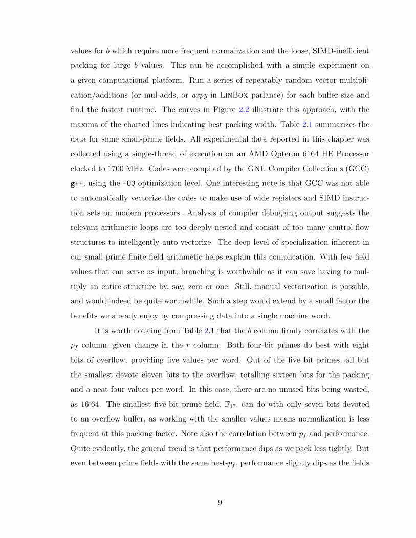
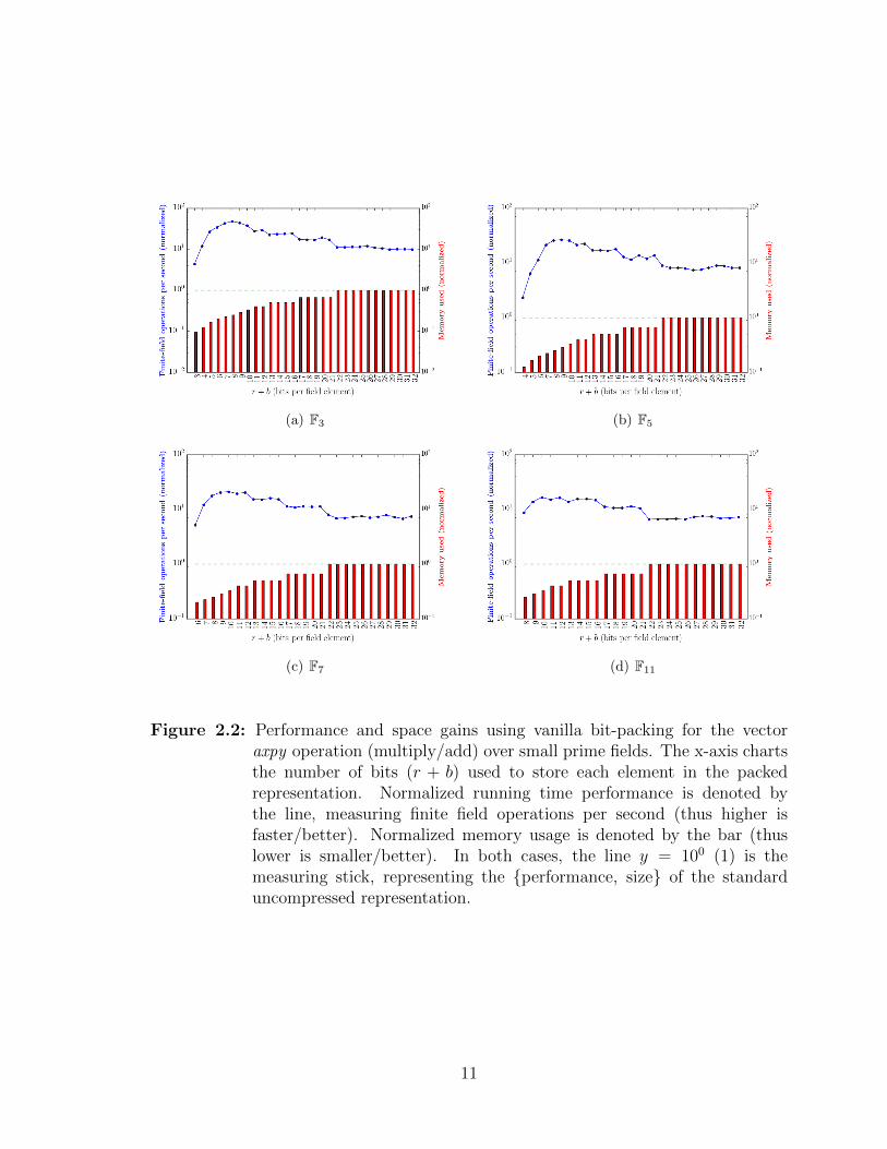
Figure 2.2 demonstrates the dual benefits of bit-packing. Each chart is organized

left-to-right from tighter to looser packings. Memory footprint is diminished consid-

erably with the tighter packings, as evidenced by the smaller bars toward the left of

the x-axes. Performance of vector operations, as depicted by the lines, is improved

by at least an order of magnitude. Each component is normalized against LinBox’s

plain−domain, the data-agnostic, and currently best, implementation for finite-field

matrix operations in LinBox. The reduction of storage space is a constant. The rela-

tive performance is a ratio of the running-times for 109 compressed to uncompressed,

but otherwise identical, finite-field operations. The computation is highly regular; over

hundreds of repetitions of the experiment, the variance between the ratios is less than

10−5.

10

(a) F3 (b) F5

(c) F7 (d) F11

Figure 2.2: Performance and space gains using vanilla bit-packing for the vectoraxpy operation (multiply/add) over small prime fields. The x-axis chartsthe number of bits (r + b) used to store each element in the packedrepresentation. Normalized running time performance is denoted bythe line, measuring finite field operations per second (thus higher isfaster/better). Normalized memory usage is denoted by the bar (thuslower is smaller/better). In both cases, the line y = 100 (1) is themeasuring stick, representing the {performance, size} of the standarduncompressed representation.

11

2.2.1 Faster bit-packing

For F3, b = 1 would be ideal from the SIMD point of view; fewer bits allotted

for overflow means more bits per word devoted to data we care about, and thus a

higher degree of inherent SIMD parallelism. However using a one-bit overflow buffer,

normalization would have to be performed after each element-wise addition or multipli-

cation, as each of these arithmetic operations has potential for bit-overflow. Therefore

performing two consecutive operations would potentially overflow the buffer. Such a

runtime-costly burden, that of normalization, works against or even fully negates the

benefits of compressing finite-field data in the first place.

To overcome the obstacle of frequent normalization while using small arithmetic

buffers is the innovation of semi-normalization [9]. Over F3 with b = 1, this technique

clears out the highest-order, buffer bit of each bit-packed finite field value whilst main-

taining data integrity, all without performing the tedious unpack-mod-pack routine

outlined above. With the “buffer bit” off, values can be doubled or added together

safely. Thus, arithmetic performed during a linear algebra routine can continue unfet-

tered by the aforementioned costly naive normalization. Semi-normalization requires

exactly four bit operations– not per element, but per machine word (or fp elements).

Essentially, the overflow bit is isolated with a bit-mask, right-shifted, and added back

into the lower-order two bits (which were isolated with a bit-mask themselves). These

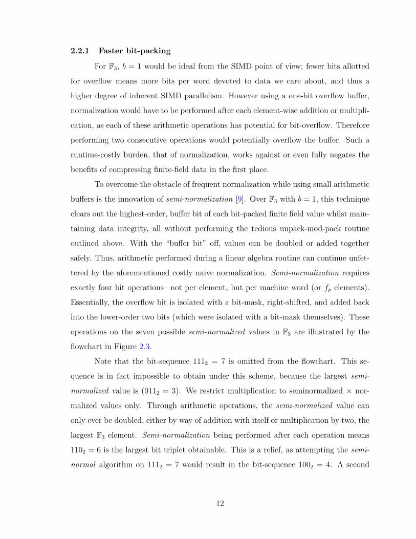
operations on the seven possible semi-normalized values in F3 are illustrated by the

flowchart in Figure 2.3.

Note that the bit-sequence 1112 = 7 is omitted from the flowchart. This se-

quence is in fact impossible to obtain under this scheme, because the largest semi-

normalized value is (0112 = 3). We restrict multiplication to seminormalized × nor-

malized values only. Through arithmetic operations, the semi-normalized value can

only ever be doubled, either by way of addition with itself or multiplication by two, the

largest F3 element. Semi-normalization being performed after each operation means

1102 = 6 is the largest bit triplet obtainable. This is a relief, as attempting the semi-

normal algorithm on 1112 = 7 would result in the bit-sequence 1002 = 4. A second

12

Figure 2.3: Flowchart depicting the four bit operations needed for semi-normalization for bit-packed F3. The seven possible 3-bit sequences thatexist whilst using semi-normalization (0002...1102) are detailed. Notethat the F3 value of each triplet of bits maintains its integrity over thisfield by the end of the routine. At finish, the highest order bit in eachset is shown to be off, which is the central concept that allows for furtherarithmetic on the packed values.

13

semi-normalization would be required to switch off the high-order bit in this case.

This second step would otherwise be required after every arithmetic operation, so not

having to perform it is a performance boon.

When true field values are called for, semi-normalized F3 values can be fully nor-

malized by converting all of the threes, the highest possible semi-normalized value, to

zeros. This operation can be done using nine bit operations per 64-bit word, in similar

fashion to the core semi-normalization routine. This is demonstrated in Algorithm 3.

Though retrieving fully-normalized, pure field elements is generally infrequently nec-

essary (for instance, only upon an algorithm’s completion), nine bit-operations is sig-

nificantly computationally faster than the naive unpack-and-mod approach given in

Algorithms 1 and 2. This tandem of specialized normalization techniques ensures the

run-time savings is commensurate with the memory-space savings that bitpacking of-

fers over uncompressed finite field storage.

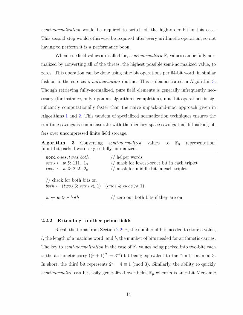
Algorithm 3 Converting semi-normalized values to F3 representation.Input bit-packed word w gets fully normalized.

word ones, twos, both // helper wordsones← w & 111...18 // mask for lowest-order bit in each triplettwos← w & 222...28 // mask for middle bit in each triplet

// check for both bits onboth← (twos & ones� 1) | (ones & twos� 1)

w ← w & ∼both // zero out both bits if they are on

2.2.2 Extending to other prime fields

Recall the terms from Section 2.2: r, the number of bits needed to store a value,

l, the length of a machine word, and b, the number of bits needed for arithmetic carries.

The key to semi-normalization in the case of F3 values being packed into two-bits each

is the arithmetic carry ((r + 1)th = 3rd) bit being equivalent to the “unit” bit mod 3.

In short, the third bit represents 22 = 4 ≡ 1 (mod 3). Similarly, the ability to quickly

semi-normalize can be easily generalized over fields Fp where p is an r-bit Mersenne

14

prime (i.e. p = 2r − 1). For these Fp, every rth bit is a “unit” bit mod p. Therefore

if your values are packed into r bits and then you perform arithmetic on the packed

values, the overflow itself acts as an additive component of the new value.

How many bits-per-value must we earmark for overflow? As shown, semi-

normalized F3 can get away with just a single bit for arithmetic carry. In general

we may wish to multiply our semi-normalized representations, which use r bits. Thus,

a further r bits are necessary to store the product (i.e. set b = r). All told, 2r bits are

required to store each packed value. Therefore to utilize SIMD bit-packing at all, it is

necessary that r ≤ l4.

This means we can specialize standard bit-packing using 64-bit words for the

following list of Mersenne prime fields: F3, F7, F31, F127, F8191. The semi-normalization

process in the general case is similar to what is done over F3, only r high-order bits

are isolated and accumulated into the r low-order “value” bits, instead of just the

single carry bit. Unlike as demonstrated for F3 in Figure 2.3, a single iteration of the

semi-normal subroutine may not be enough to clear the high-order “carry” bits to be

all zeroes. Performing this process once is sufficient following any addition operation,

but following a multiplication it is possible that this action would again overflow the

“value” bits. However we are in luck, the semi-normalization operation is idempotent,

and can simply be applied once more, to assuredly clear the b high-order “carry” bits.

All of this sums to eight bit-operations per machine-word of packed values, as each

iteration of semi-normalization still requires four bit-operations.

The isolation of the high- and low- order bits is accomplished with yet another

bit-mask. By way of example, in the case of F7 we can mask the three high-order

“carry” bits out of the six-bits-per-element with a mask of 708. We start with these

six bits and repeat them– going right-to-left– to arrive at a 64-length bit-mask of

707070707070707070708. For completeness, the low order bits are masked with an

inverse mask 070707070707070707078. The general semi-normalization algorithm is

outlined in Algorithm 4. These masks will be referred to in the pseudocode as MASK HI

and MASK LO, respectively.

15

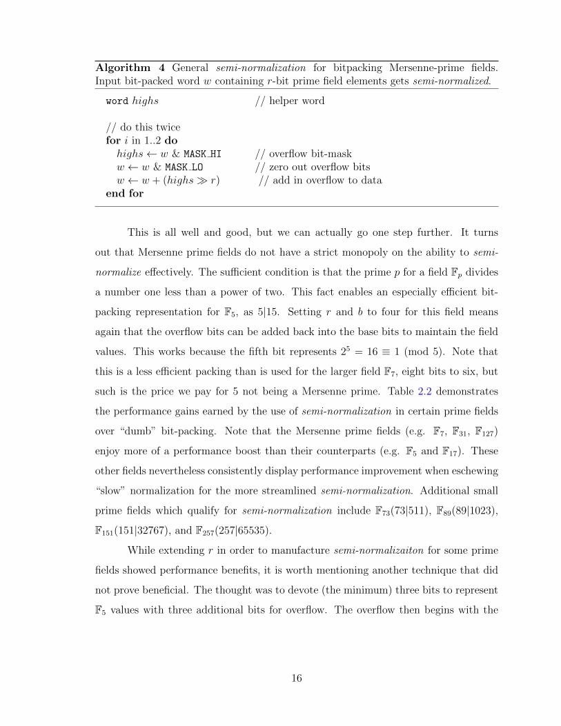
Algorithm 4 General semi-normalization for bitpacking Mersenne-prime fields.Input bit-packed word w containing r-bit prime field elements gets semi-normalized.

word highs // helper word

// do this twicefor i in 1..2 dohighs← w & MASK HI // overflow bit-maskw ← w & MASK LO // zero out overflow bitsw ← w + (highs� r) // add in overflow to data

end for

This is all well and good, but we can actually go one step further. It turns

out that Mersenne prime fields do not have a strict monopoly on the ability to semi-

normalize effectively. The sufficient condition is that the prime p for a field Fp divides

a number one less than a power of two. This fact enables an especially efficient bit-

packing representation for F5, as 5|15. Setting r and b to four for this field means

again that the overflow bits can be added back into the base bits to maintain the field

values. This works because the fifth bit represents 25 = 16 ≡ 1 (mod 5). Note that

this is a less efficient packing than is used for the larger field F7, eight bits to six, but

such is the price we pay for 5 not being a Mersenne prime. Table 2.2 demonstrates

the performance gains earned by the use of semi-normalization in certain prime fields

over “dumb” bit-packing. Note that the Mersenne prime fields (e.g. F7, F31, F127)

enjoy more of a performance boost than their counterparts (e.g. F5 and F17). These

other fields nevertheless consistently display performance improvement when eschewing

“slow” normalization for the more streamlined semi-normalization. Additional small

prime fields which qualify for semi-normalization include F73(73|511), F89(89|1023),

F151(151|32767), and F257(257|65535).

While extending r in order to manufacture semi-normalizaiton for some prime

fields showed performance benefits, it is worth mentioning another technique that did

not prove beneficial. The thought was to devote (the minimum) three bits to represent

F5 values with three additional bits for overflow. The overflow then begins with the

16

Figure 2.4: Figure 2.2(c), detailing bit-packing for F7, updated with a data point(denoted by ×) where semi-normalization is employed. The best of allworlds is achieved: faster than the fastest bit-packed time (line) pairedwith the smallest possible memory usage (bars).

17

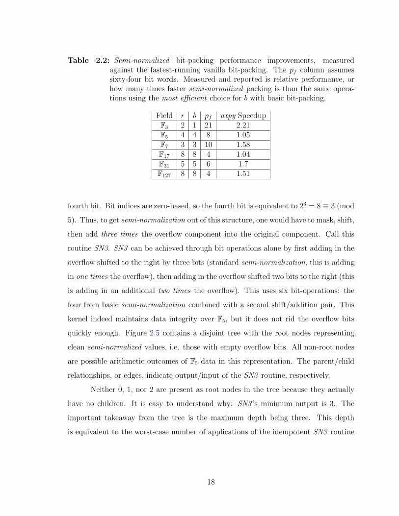
Table 2.2: Semi-normalized bit-packing performance improvements, measuredagainst the fastest-running vanilla bit-packing. The pf column assumessixty-four bit words. Measured and reported is relative performance, orhow many times faster semi-normalized packing is than the same opera-tions using the most efficient choice for b with basic bit-packing.

Field r b pf axpy SpeedupF3 2 1 21 2.21F5 4 4 8 1.05F7 3 3 10 1.58F17 8 8 4 1.04F31 5 5 6 1.7F127 8 8 4 1.51

fourth bit. Bit indices are zero-based, so the fourth bit is equivalent to 23 = 8 ≡ 3 (mod

5). Thus, to get semi-normalization out of this structure, one would have to mask, shift,

then add three times the overflow component into the original component. Call this

routine SN3. SN3 can be achieved through bit operations alone by first adding in the

overflow shifted to the right by three bits (standard semi-normalization, this is adding

in one times the overflow), then adding in the overflow shifted two bits to the right (this

is adding in an additional two times the overflow). This uses six bit-operations: the

four from basic semi-normalization combined with a second shift/addition pair. This

kernel indeed maintains data integrity over F5, but it does not rid the overflow bits

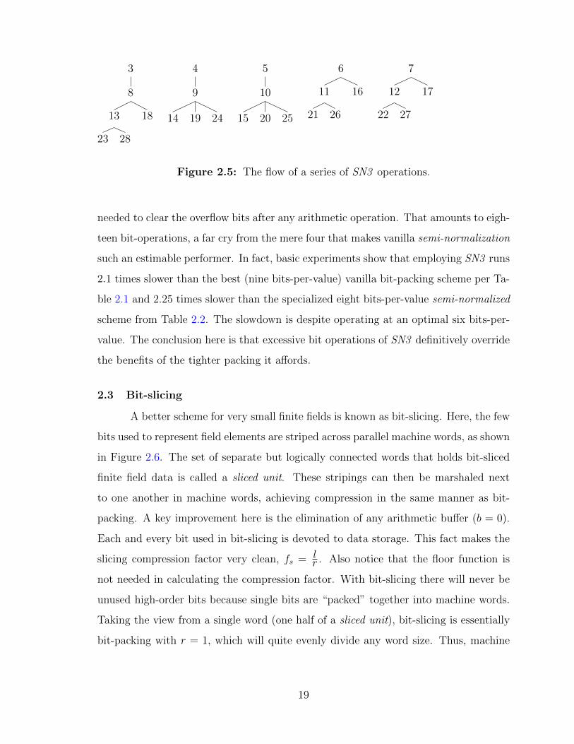
quickly enough. Figure 2.5 contains a disjoint tree with the root nodes representing

clean semi-normalized values, i.e. those with empty overflow bits. All non-root nodes

are possible arithmetic outcomes of F5 data in this representation. The parent/child

relationships, or edges, indicate output/input of the SN3 routine, respectively.

Neither 0, 1, nor 2 are present as root nodes in the tree because they actually

have no children. It is easy to understand why: SN3 ’s minimum output is 3. The

important takeaway from the tree is the maximum depth being three. This depth

is equivalent to the worst-case number of applications of the idempotent SN3 routine

18

3

8

13

23 28

18

4

9

14 19 24

5

10

15 20 25

6

11

21 26

16

7

12

22 27

17

Figure 2.5: The flow of a series of SN3 operations.

needed to clear the overflow bits after any arithmetic operation. That amounts to eigh-

teen bit-operations, a far cry from the mere four that makes vanilla semi-normalization

such an estimable performer. In fact, basic experiments show that employing SN3 runs

2.1 times slower than the best (nine bits-per-value) vanilla bit-packing scheme per Ta-

ble 2.1 and 2.25 times slower than the specialized eight bits-per-value semi-normalized

scheme from Table 2.2. The slowdown is despite operating at an optimal six bits-per-

value. The conclusion here is that excessive bit operations of SN3 definitively override

the benefits of the tighter packing it affords.

2.3 Bit-slicing

A better scheme for very small finite fields is known as bit-slicing. Here, the few

bits used to represent field elements are striped across parallel machine words, as shown

in Figure 2.6. The set of separate but logically connected words that holds bit-sliced

finite field data is called a sliced unit. These stripings can then be marshaled next

to one another in machine words, achieving compression in the same manner as bit-

packing. A key improvement here is the elimination of any arithmetic buffer (b = 0).

Each and every bit used in bit-slicing is devoted to data storage. This fact makes the

slicing compression factor very clean, fs = lr . Also notice that the floor function is

not needed in calculating the compression factor. With bit-slicing there will never be

unused high-order bits because single bits are “packed” together into machine words.

Taking the view from a single word (one half of a sliced unit), bit-slicing is essentially

bit-packing with r = 1, which will quite evenly divide any word size. Thus, machine

19

r = 2

{011010100

|0

bit-sliced value (0)

0110110100100010|1

bit-sliced value (1)

0101010101010100000|1

bit-sliced value (2)

01011111010111

0100101000100110000100000000010001010101000000101010101011000︸ ︷︷ ︸l = 64

Figure 2.6: A closeup of two machine words utilizing bit-slicing to store F3 values. Wecall this pair of words a sliced unit. This is followed by a broad view of thesavings bit-slicing affords. The rectangular outlines represent machinewords while the shaded portions represent finite field data. Notice thatthe colors, representing individual finite field values, are striped in parallelfashion between the two bit-sliced words. Two words are used to storewhat would take sixty-four without the compression.

words comprising vectors of bit-sliced data can always be filled out completely. This

is in contrast to bit-packing, where high-order bits remain unused when (r + b) - l.

Algorithm 5 demonstrates the insertion of a finite field value into a bit-sliced

vector. Once again we notice that converting uncompressed data to our specialized

representation is computationally costly. And once again we assert that there is plenty

of value in the scheme despite this stipulation. The benefits of performing arithmetic

in bulk with the compressed representation vastly outweigh the costs in arriving at

the compression. Insertion of a value into sliced form is accomplished by pinpointing

20

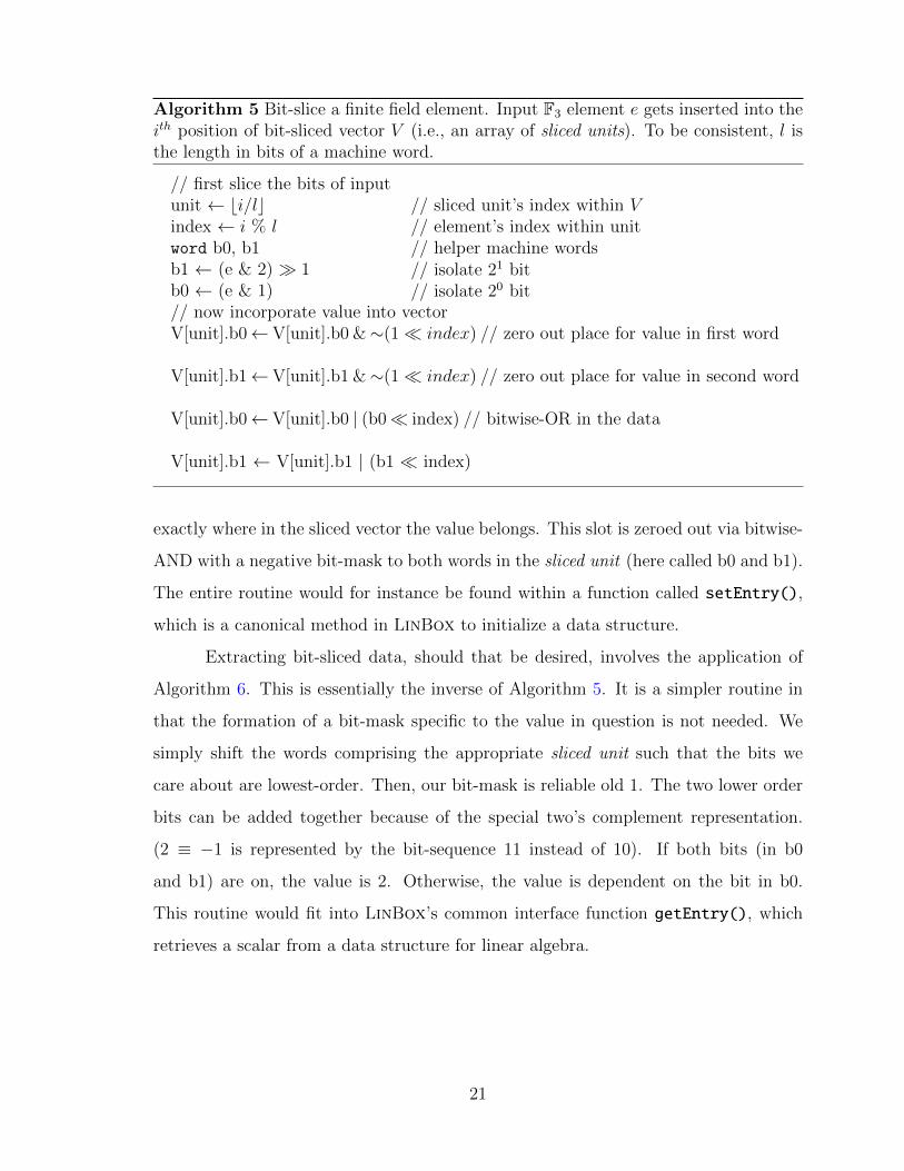
Algorithm 5 Bit-slice a finite field element. Input F3 element e gets inserted into theith position of bit-sliced vector V (i.e., an array of sliced units). To be consistent, l isthe length in bits of a machine word.

// first slice the bits of inputunit ← bi/lc // sliced unit’s index within Vindex ← i % l // element’s index within unitword b0, b1 // helper machine wordsb1 ← (e & 2) � 1 // isolate 21 bitb0 ← (e & 1) // isolate 20 bit// now incorporate value into vectorV[unit].b0←V[unit].b0 &∼(1� index) // zero out place for value in first word

V[unit].b1←V[unit].b1 &∼(1� index) // zero out place for value in second word

V[unit].b0←V[unit].b0 | (b0� index) // bitwise-OR in the data

V[unit].b1 ← V[unit].b1 | (b1 � index)

exactly where in the sliced vector the value belongs. This slot is zeroed out via bitwise-

AND with a negative bit-mask to both words in the sliced unit (here called b0 and b1).

The entire routine would for instance be found within a function called setEntry(),

which is a canonical method in LinBox to initialize a data structure.

Extracting bit-sliced data, should that be desired, involves the application of

Algorithm 6. This is essentially the inverse of Algorithm 5. It is a simpler routine in

that the formation of a bit-mask specific to the value in question is not needed. We

simply shift the words comprising the appropriate sliced unit such that the bits we

care about are lowest-order. Then, our bit-mask is reliable old 1. The two lower order

bits can be added together because of the special two’s complement representation.

(2 ≡ −1 is represented by the bit-sequence 11 instead of 10). If both bits (in b0

and b1) are on, the value is 2. Otherwise, the value is dependent on the bit in b0.

This routine would fit into LinBox’s common interface function getEntry(), which

retrieves a scalar from a data structure for linear algebra.

21

Algorithm 6 Extracting finite field element data from a bit-sliced representation.Output F3 element e gets the ith value in bit-sliced vector V .

unit ← bi/lc // sliced unit’s index within Vindex ← i % l // element’s index within unit// perform extraction from both words in the proper unite ← (V[word].b1 � index) & 1 + (V[word].b0 � index) & 1

2.3.1 Specialized arithmetic

Devoting no storage space for arithmetic overflow is quite convenient. Of course

this makes storage more efficient, as every bit is devoted to the data itself. On top of

that the burdensome normalization required by bit-packing is rendered entirely unnec-

essary. It seems too good to be true; just how is this accomplished? Well, the large

caveat here is that specialized arithmetic is required on a per-field basis– an arith-

metic engineered from the ground up to avoid carries. This problem is equivalent to

circuit minimization across a truth table of an r-variate Boolean function describing

the mapping from binary inputs and outputs across an arithmetic operation. The size

of the circuit is the number of bit-operations needed to perform the arithmetic. This

problem is computationally NP-Indeterminate, and in practice quite difficult. Hence

this scheme is only practical for very small prime fields where custom arithmetic can

be worked out.

For instance, also given by [5], in F3 regular addition (Algorithm 7) requires

only six bitwise operations per pair of words. This can be done using the following rep-

resentation for F3 values: 0 = 002, 1 = 102,−1 = 112. Negation (Algorithm 8), which

is in this field is equivalent to multiplication by 2 ≡ −1, requires only one bitwise

operation. Trivially applying addition and negation, subtraction can be accomplished

in seven bit operations. However, a different formula exists for subtraction in just six.

Multiplication by 2 ≡ −1 is the only non trivial multiplicand for this field; multiplica-

tion by zero simply empties the sliced words, and multiplication by one is a no-op. In

Algorithms 7 and 8, the accessors “bit0” and “bit1” respectively refer to the words of

the sliced units that hold the lower order bits (those switching 20 in the field element)

22

and the high order bits (those switching 21). Similarly clever games can be played with

certain subsets of arithmetic in F5, F7, and some extension fields of small prime fields.

Please see [5] for further discussion of bit-slicing for those fields, as they are not a focus

of this thesis. The application contained in Chapter 3 concerns F3 bit-slicing, so this

is the only field for which we implemented bit-slicing in LinBox thus far.

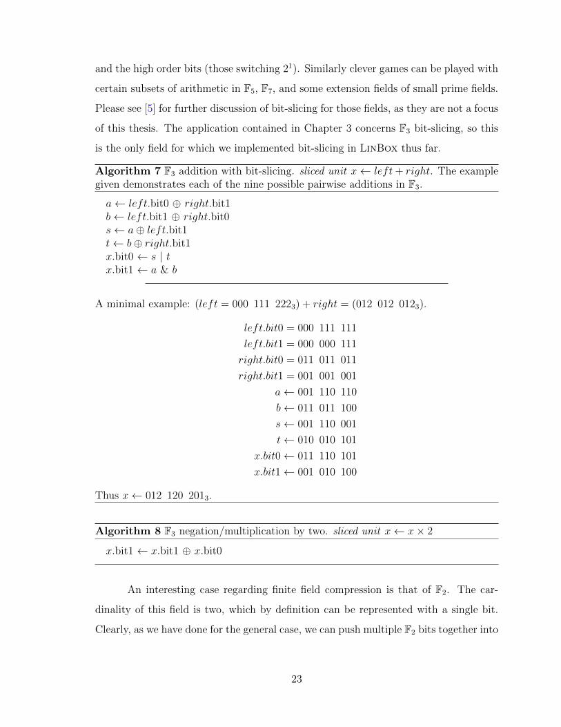
Algorithm 7 F3 addition with bit-slicing. sliced unit x← left+ right. The examplegiven demonstrates each of the nine possible pairwise additions in F3.

a← left.bit0 ⊕ right.bit1b← left.bit1 ⊕ right.bit0s← a⊕ left.bit1t← b⊕ right.bit1x.bit0 ← s | tx.bit1 ← a & b

A minimal example: (left = 000 111 2223) + right = (012 012 0123).

left.bit0 = 000 111 111

left.bit1 = 000 000 111

right.bit0 = 011 011 011

right.bit1 = 001 001 001

a← 001 110 110

b← 011 011 100

s← 001 110 001

t← 010 010 101

x.bit0← 011 110 101

x.bit1← 001 010 100

Thus x← 012 120 2013.

Algorithm 8 F3 negation/multiplication by two. sliced unit x← x× 2

x.bit1 ← x.bit1 ⊕ x.bit0

An interesting case regarding finite field compression is that of F2. The car-

dinality of this field is two, which by definition can be represented with a single bit.

Clearly, as we have done for the general case, we can push multiple F2 bits together into

23

Figure 2.7: Figure 2.2(a), detailing F3 compression, updated with two data points:semi-normalized bit-packing denoted by × and bit-slicing denoted by +.Bit-slicing being the optimal compression scheme for F3 is quite evident,as it more than doubles the performance of the best (semi-normalized)bit-packing. On top of this, it uses the optimal two bits per finite fieldelement, so it is also the most efficient compression scheme from a memo-ry/storage standpoint, using 6.25% of the memory of the naive approach.

24

single machine words. When we do this, we are in fact simultaneously achieving both

bit-packing and bit-slicing! Adding two F2 sliced units is simple: bitwise-XOR them.

Multiplying two F2 sliced units is equally simple: bitwise-AND them. Component-

wise sliced unit multiplication is not something currently provided by F3 bit-slicing in

LinBox. F2 matrix-vector product is accomplished by word-wise bitwise-AND between

matrix rows and vector, then an accumulation of these words with bitwise-XOR. The

parity of the word resulting from this accumulation is the matrix-vector product for

the given row. Sub-cubic matrix-matrix multiplication is possible as an extension of

this method. Also detailed by Albrecht, et al. [6] are other very fast matrix-matrix

multiplication routines over F2, Strassen-Winograd and the Method of Four Russians.

2.4 Summary

The most attractive attribute of bit-packing is its flexibility. Any field with the

property r ≤ l4 for a given machine can utilize bit-packing. Bit-packing has memory

savings and arithmetic efficiency built in; when you use it, your program runs faster

and smaller. Additionally, some small prime fields can take advantage of the specialized

semi-normalized variant to squeeze out even more runtime savings.

Bit-slicing however, is the clear-cut best compression scheme when compact,

custom no-carry bit arithmetic can be worked out for the desired finite field. Therein

lies the rub, but such is certainly the case for compressing F3. F3 bit-slicing far out-

performs even the formidable semi-normalized edition of F3 bit-packing. It also uses

23 the data storage that even the tightest bit-packing needs. When computing with

matrices or vectors containing entries over F3, always use bit-slicing.

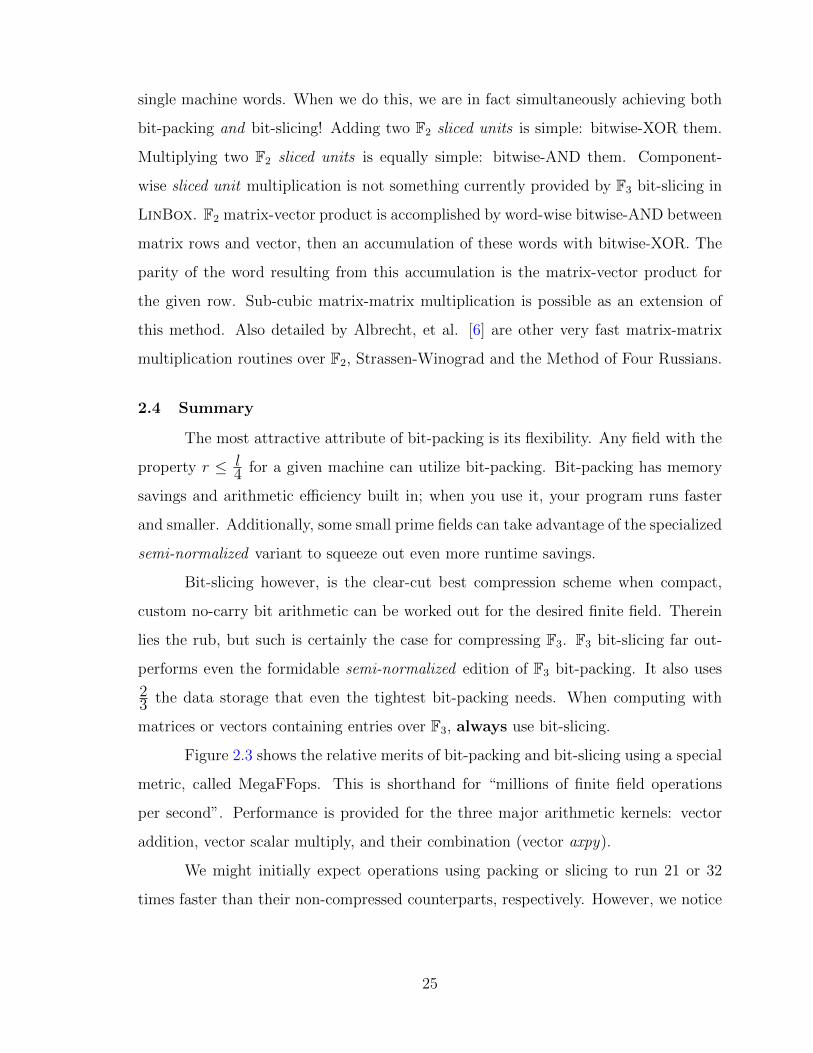
Figure 2.3 shows the relative merits of bit-packing and bit-slicing using a special

metric, called MegaFFops. This is shorthand for “millions of finite field operations

per second”. Performance is provided for the three major arithmetic kernels: vector

addition, vector scalar multiply, and their combination (vector axpy).

We might initially expect operations using packing or slicing to run 21 or 32

times faster than their non-compressed counterparts, respectively. However, we notice

25

Table 2.3: Speed of vector operations over F3, using elements that are a) stored asfloats and using BLAS, b) stored as ints, c) packed, and d) sliced. Timingsof arithmetic were done on random vectors of length 107.

F3 Arithmetic Comparison (MegaFFops)Operation float int packed slicedadd x+ y 120.65 165.9 4492 6100

scalar mul αx 81.15 136.5 21008 65112axpy αx+ y 77.96 98.46 6165 8806

improvement much better than that in the experiment of adding two vectors. Multi-

plying a vector by a random scalar from the field is an even more impressive win for the

bit-packed and bit-sliced representations. Here we may be seeing memory hierarchy

benefits from compressing to a smaller memory footprint. Also helping is the high level

of specialization our compression schemes provide that the other implementations lack.

With bit-packing we use only a single bit shift to accomplish multiplication by two, fol-

lowed by semi-normalization. With bit-slicing we again employ a single bit-operation

with no need for normalization. Axpy runs slightly faster than addition. This is an

encouraging sign, considering addition is part of axpy. The ground gained on addition

is explained by the third of the time where the random multiplication scalar is zero

and no addition is necessary.

In conclusion, the suite of bit-packing and bit-slicing greatly improves efficiency

of arithmetic in small prime finite fields. Having faster arithmetic in these fields benefits

many of the kernels in LinBox. For example Dumas and Villard highlight many

applications for exact computation using small finite fields in [10]. The applications

listed there, including factoring large integers, computing Smith form, and homology

all stand to improve with the new compressions. In Chapter 3 we will discuss a specific

problem that has certainly benefited, if not outright relied upon, bit-slicing for F3.

26

Chapter 3

STRONGLY REGULAR GRAPH 3-RANKS

3.1 Introduction

Matrix rank has been perhaps the most widely used exact linear algebra com-

putation to date. It has often been the goal of computations requested by users of the

LinBox software library for exact linear algebra computations over the integers and

over finite fields. Besides being of interest itself in numerous applications, rank plays

an important role in solving singular systems and computing invariants. For example

the rank is used in solving large sparse linear systems [11] computing homology groups

[12], and in computation of Grobner bases [13].

The goal for this chapter is to compute the ranks in a sequence of adjacency

matrices of strongly regular graphs as defined by Dickson and detailed by Xiang et al.

in [14]. We will refer to the matrices in the Dickson graph sequence as D(p, e) : e ∈ N,

where p is a prime number. Of specific interest to us is p = 3, where the matrices consist

of entries over F3. The 3-rank is sought, meaning all arithmetic is also done over F3.

The rank of D(3, e) has been previously computed for e ∈ 1 . . . 6, e.g. in [15, 16, 14].

More recently we obtained the rank of D(3, 7) [9], which evinced a conjecture that

the rank of D(3, 8) could help confirm. The difficulty in computing the 3-ranks for

D(3, 7) and D(3, 8) stems from the sheer volume of data these matrices contain. Each

Dickson adjacency matrix is p2e × p2e, however the ranks are considerably smaller, on

the order of 22e+1. Thus, D(3, 7) contains (314)2 ≈ 22.9 tera-entries, but only a rank

near 215 ≈ 32000 is expected. Similarly D(3, 8) contains (316)2 ≈ 1.85 peta-entries,

with expected rank near 217 ≈ 131000. The small rank estimate nudges this problem

into being practically solvable by current computing resources. The basic idea is to

27

losslessly compress the larger matrix into a roughly rank-sized block, on which to do

final, classical rank computations. “Small” rank notwithstanding, this is enough data

to present considerable challenges not just in computing the rank, but also in merely

generating, representing, and storing the Dickson matrix itself.

This chapter will highlight these challenges, after beginning with the methodol-

ogy of solving for the rank of D(3, 7). Specialized bit-packing was used by the original

computation [9], but bit-slicing has been the compression of choice for more recent du-

plicate computations. Construction for the Dickson family of matrices will be detailed.

Following will be an exploration of techniques used in solving for the rank of D(3, 8).

A matrix decomposition strategy is required due to the volume of data stored in the

matrix. Different data-decomposition strategies were attempted with varying degrees

of success. Before detailing what ultimately worked, a failed attempt at solving the

problem is outlined; often failures can be just as illuminating and worthy of discussion

as successes.

Naturally given the decomposed nature of the matrix data, some well-known

distributed and shared-memory parallel computing mechanisms were deployed to gen-

erate a compressed form of the matrix. Shared-memory parallelism was also used in

the rank algorithm on this compressed form. Bit-slicing was employed throughout the

computation, vastly improving arithmetic efficiency over F3. Recall the infrastructure

of bit-slicing instantly provides chip-level data parallelism. Finally, there is still room

to expand; the methods presented here are both applicable to, and foundational for

computing a suite of related problems. In this light, a discussion of potential directions

for this strong base of work to grow is included.

In this chapter log is base 2.

3.1.1 Prior work

There are various well-studied approaches for computing the rank of a matrix.

Singular value decomposition is a common approach on matrices containing real or

complex numbers that is not applicable here due to the finite-field arithmetic needed.

28

Two common approaches are found in exact linear algebra: classical Gaussian elimi-

nation or LU -decomposition [17], and probabilistic blackbox methods, for example the

Wiedemann approach [18, 19]. From a complexity point of view, for an n × n dense

matrix of rank r, the rank may be computed in O(rn2) field operations and storage of

n2 field elements, using Gaussian elimination. Blackbox methods can be run in time

O (rn2), using O (n) storage. Here we use O () to mean we ignore log factors. In

particular, for rank over a small field, this notation hides the necessity to work over an

extension field of degree O(log(n) log(1/ε)), where ε denotes the desired upper bound

on the probability of failure of the Monte Carlo algorithm. This is in order to have suf-

ficiently many elements for the random choices. Also the blackbox approach requires

accessing each entry of the matrix O(2r) times, which is costly for the too-large-to-

store but entry-on-demand-by-formula matrices of our intended application. In the

paper of May, Saunders, and Wan on this topic [15] several Monte Carlo algorithms

that run in time O (rn2) and require varying amounts of memory were reported and

used on the Dickson matrices. The algorithm discussed in Section 3.2.1 improves the

time complexity to O (n2) and storage to O(r2) (beyond the requirement to access

each matrix entry exactly once). Also given is a Monte Carlo certification algorithm

that is useful for verifying rank after use of heuristics. It is simpler and of lower space

and time costs than the certificates of prior work [15]. While the prior work done on

this topic provided the basic structure for computing the ranks of the large Dickson

matrices, the improvements that follow in this chapter have made the computation

itself readily possible.

3.2 Obtaining rank(D(3, 7))

D(3, 7) is understandably a challenge computationally in view of the fact that its

storage would require over 22 terabytes at one byte per entry. Each entry of D(3, 7) is

determined by a straightforward but somewhat expensive formula involving arithmetic

in F37 . Fortunately, it is not necessary to work with the completely constructed matrix

at one time. We have found it effective to work at any one time with about one billion

29

entries, roughly one part in 20,000 of the matrix. We gain efficiency of both space and

time by employing either specialized F3 bit-packing or bit-slicing.

3.2.1 Space and time efficient p-Rank

For this section let A be an n× n matrix of rank r over a finite field K. If A is

large and dense and yet the rank is small, how may we compute rank(A) efficiently?

We present a method that is a Monte Carlo algorithm for large enough fields and

runs in O (n2 + r3) time and using O(r2) space. This is essentially optimal when r ∈

O(n2/3). Here “O ()” and “essentially” mean that we ignore log factors. Independently,

a very similar observation concerning optimality of matrix operations in a low rank

setting has been made by Kaltofen [20], who showed optimality of an algorithm for

system solving for sufficiently over- or under-determined systems. We also give a Monte

Carlo certificate that works for all fields, and is important to the 3-rank computation

discussed in the following section. This uses random linear combinations of rows and

columns, a projection technique that was also used for handling low rank matrices by

Cooperman and Havas [21].

The main idea of our rank algorithm is to use butterfly preconditioners. We

know that if B and C are butterfly matrices, then the matrix BAC has generic rank

profile with high probability [22, 23]. Generic rank profile means the leading principal

minors are nonzero up to the rank. A leading principal minor, order k, of a matrix order

n is the leading k×k block, obtained by deleting the last (n−k) rows and columns from

the matrix. One could imagine trying to compute larger and larger leading principal

minors until a zero minor is encountered. This is precisely one of the earlier methods

[24, 22], but it requires too much time and space for our current problems. Let us set

out to achieve a helpful leading submatrix with nonsingular leading principal minors

by another means. We propose a sum of blocks, with each block preconditioned. Let

b be the block size, a number to be discussed further. For now keep in mind that the

30

goal will be that b is slightly larger than the rank of the matrix. Consider

M =∑i∈0..n

b

∑j∈0..n

b

BiAi,jCj,

where all terms are b × b matrices, Ai,j being the block in the i-th row of blocks and

j-th column of blocks in a partitioning of A into b × b blocks. This will create an

advantage of small space and time requirement. Only one block of A is needed in

memory at a time so the algorithm requires a block of A, a block for the partial sum,

and whatever storage is required for the preconditioning blocks, the Bi and Cj. The

runtime is evidently O((nb)2(b2 +T (b))) field operations, where (n

b)2 counts the number

of summands, the b2 represents the cost of adding one block, and T(b) is the cost of

preconditioning (the operations to produce a product BiAi,jCj). The memory cost is

for storage of M (as a partial sum during the algorithm), and one block of A at any

one time, so O(b2) for these entries. The storage cost is then O(b2 + (nb)S(b))), where

b2 accounts for storing one block of A and (a partial sum of) M at any one time, with

2nb

preconditioning blocks (Bi and Cj) at space S(b) each. It will turn out that T(b) is

O(b2 log(b)) and S(b) is O(b log(b)), because the preconditioners are butterfly matrices

(discussed next). Then we have overall costs of O(n2 log(b)) time and O(n log(b)) space

for the construction of M . We can then efficiently compute the rank of M � A.

When b is a power of 2, a b × b butterfly matrix is a product of log(b) stage

matrices each of which is a direct sum of b2

two-by-two switches. The direct sums are

organized so that in the i-th stage there is a switch for each pair of rows and columns

whose indices, expressed in binary notation, differ only at the ith bit.

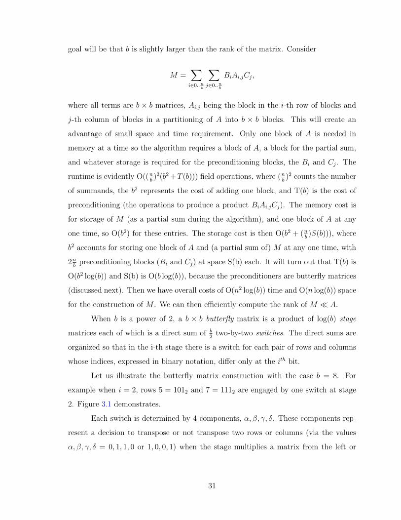
Let us illustrate the butterfly matrix construction with the case b = 8. For

example when i = 2, rows 5 = 1012 and 7 = 1112 are engaged by one switch at stage

2. Figure 3.1 demonstrates.

Each switch is determined by 4 components, α, β, γ, δ. These components rep-

resent a decision to transpose or not transpose two rows or columns (via the values

α, β, γ, δ = 0, 1, 1, 0 or 1, 0, 0, 1) when the stage multiplies a matrix from the left or

31

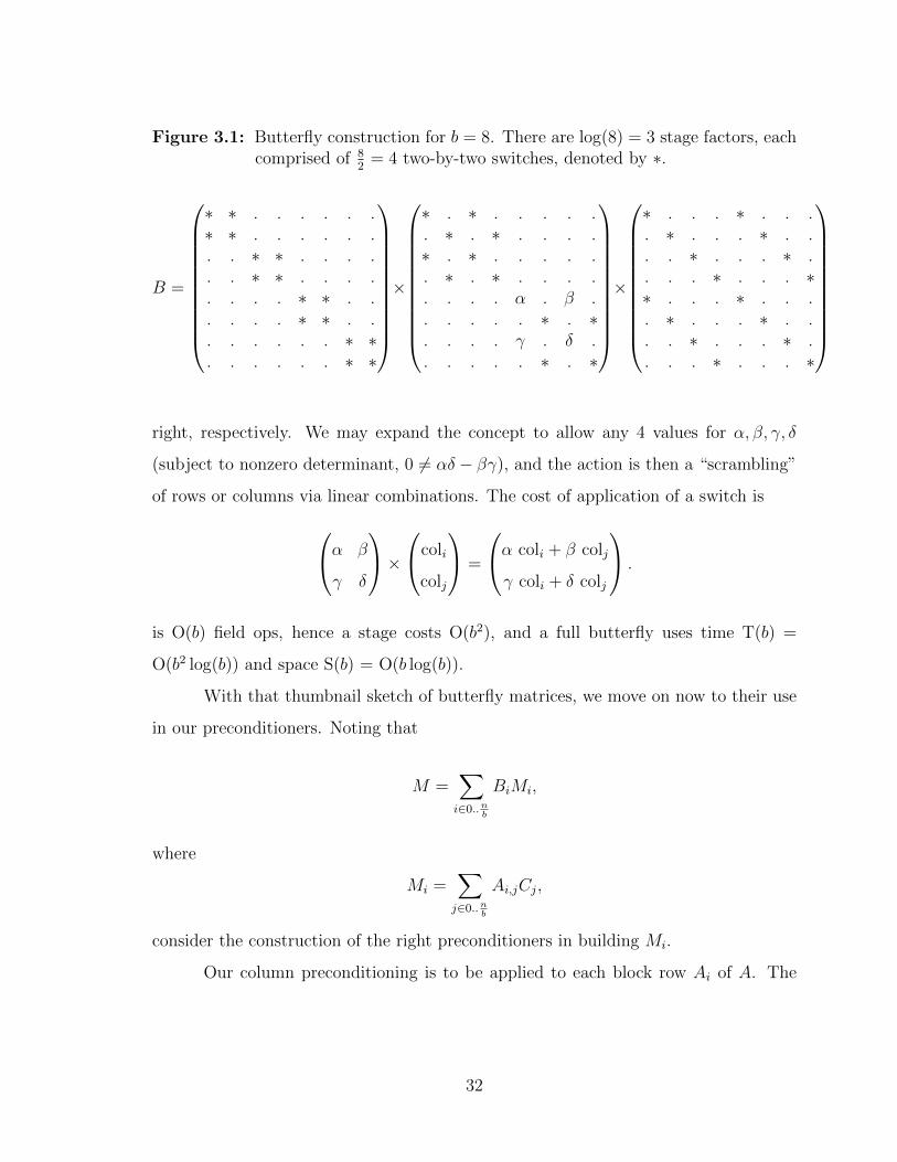
Figure 3.1: Butterfly construction for b = 8. There are log(8) = 3 stage factors, eachcomprised of 8

2= 4 two-by-two switches, denoted by ∗.

B =

∗ ∗ . . . . . .∗ ∗ . . . . . .. . ∗ ∗ . . . .. . ∗ ∗ . . . .. . . . ∗ ∗ . .. . . . ∗ ∗ . .. . . . . . ∗ ∗. . . . . . ∗ ∗

×

∗ . ∗ . . . . .. ∗ . ∗ . . . .∗ . ∗ . . . . .. ∗ . ∗ . . . .. . . . α . β .. . . . . ∗ . ∗. . . . γ . δ .. . . . . ∗ . ∗

×

∗ . . . ∗ . . .. ∗ . . . ∗ . .. . ∗ . . . ∗ .. . . ∗ . . . ∗∗ . . . ∗ . . .. ∗ . . . ∗ . .. . ∗ . . . ∗ .. . . ∗ . . . ∗

right, respectively. We may expand the concept to allow any 4 values for α, β, γ, δ

(subject to nonzero determinant, 0 6= αδ − βγ), and the action is then a “scrambling”

of rows or columns via linear combinations. The cost of application of a switch isα β

γ δ

×coli

colj

=

α coli + β colj

γ coli + δ colj

.

is O(b) field ops, hence a stage costs O(b2), and a full butterfly uses time T(b) =

O(b2 log(b)) and space S(b) = O(b log(b)).

With that thumbnail sketch of butterfly matrices, we move on now to their use

in our preconditioners. Noting that

M =∑i∈0..n

b

BiMi,

where

Mi =∑j∈0..n

b

Ai,jCj,

consider the construction of the right preconditioners in building Mi.

Our column preconditioning is to be applied to each block row Ai of A. The

32

argument applies to column operations performed on any matrix, so we simplify nota-

tion by referring to A rather than Ai. We have A partitioned into blocks of columns.

The block size b should be no less than the rank. Later we will address how to find

such a block size. Assume b|n so that there are nb

blocks of size b with r < b. If n is

not a multiple of b, pad A with zero columns until this property is true.

We operate to achieve a matrix of the same rank whose leading r columns

are independent. The argument style is the familiar one of considering the random

preconditioners as random evaluations of correspondingly structured polynomial matrix

preconditioners in which the random values have become independent variables. The

first step of the argument is to show there exists an evaluation of the polynomial

matrices with desired properties. The second step (via Zippel-Schwartz [25, 26]) is to

show the desired property is to be expected when random values replace the variables.

The structure of our construction is select-permute-sum. Each preconditioning

block is of the form Ci = DiUi, where Di is diagonal and Ui is a butterfly, for i ∈

1..nb. The n diagonal entries and (n

b)(b log(b)) butterfly nonzero entries are distinct

independent variables over K. In the existence-proving step of the argument we assign

either 0 or 1 to each variable.

First, let us suppose we have identified r columns which are independent. This

is possible and our columns will form a basis for the column space, since r = rank(A).

We multiply from the right by a diagonal matrix D which has 1’s in in the diagonal

positions corresponding to the desired columns and zeroes everywhere else. Then AD

has the designated r columns the same as A’s and all other columns zero. View D

as partitioned into diagonal blocks Di which select those of the designated i columns

lying in the i-th column block of A.

33

To illustrate, we may have selected thus (vertical bars used to separate blocks):

0 ∗ 0 0 0 0

0 ∗ 0 0 0 0...

......

......

...

0 ∗ 0 0 0 0

∣∣∣∣∣∣∣∣∣∣∣∣

∗ ∗ 0 0 0 ∗

∗ ∗ 0 0 0 ∗...

......

......

...

∗ ∗ 0 0 0 ∗

∣∣∣∣∣∣∣∣∣∣∣∣

0 ∗ 0 0 0 0

0 ∗ 0 0 0 0...

......

......

...

0 ∗ 0 0 0 0

.

Let bj denote the number of designated columns in block j, and let cj denote the

prefix sum, cj =∑

i∈1..j bi. We permute the columns so that the designated columns in

block j are moved to the contiguous area in positions (cj−1 + 1)..cj (with c0 = 0). Call

such a permutation a scramble (so named because we will soon move from a specified

permutation to a randomized linear combination process). We have scrambled:

∗ 0 0 0 0 0

∗ 0 0 0 0 0...

......

......

...

∗ 0 0 0 0 0

∣∣∣∣∣∣∣∣∣∣∣∣

0 ∗ ∗ ∗ 0 0

0 ∗ ∗ ∗ 0 0...

......

......

...

0 ∗ ∗ ∗ 0 0

∣∣∣∣∣∣∣∣∣∣∣∣

0 0 0 0 ∗ 0

0 0 0 0 ∗ 0...

......

......

...

0 0 0 0 ∗ 0

Finally, we sum the blocks obtaining a n× b matrix of the same rank as A:

∗ ∗ ∗ ∗ ∗ 0

∗ ∗ ∗ ∗ ∗ 0...

......

......

...

∗ ∗ ∗ ∗ ∗ 0

Analogously, if we applied the same select-scramble-sum process on the left

(acting on the rows of this n× b matrix, we would achieve a b× b matrix with leading

r × r minor nonsingular. The left and right preconditioning multipliers are products

of 0,1 matrices (a diagonal, a permutation, and a stack of b × b identity matrices for

the summing).

The desired permutations, moving a designated set of objects to a specified

34

contiguous block, can be achieved by butterfly permutation matrices. See Lemma 5.1

in [22].

Intuitively the benefit of butterfly preconditioners with random values in the

switches is that they quite thoroughly scramble things up (getting one to an approx-

imation of the generic case where nonsingularity of the leading r × r minor is to be

expected) while being economical to use (costing O(b2 log(b)) field ops to multiply with

a dense block). This cost results from the application of log(b) stages, each calling for

b row or column operations. When the set of values from which the switch entries

are chosen at random is large enough, the probability that the preconditioned matrix

has generic rank profile (leading principal minors nonzero up to the rank) is high [22].

Thus for these preconditioners, T(b) is O(b2 log(b)) and S(b) is O(b log(b)), as stated

for these complexities earlier. Note that the diagonal block factor is absorbed in this

complexity, being of lower cost, O(b2) time and O(b) space.

To prepare for the use of randomness we turn to consider what we have if we

populate the diagonal selectors and butterfly switches with independent variables.

Theorem 1. Let K be a field and let A be an n×n matrix of rank r, where n is a power

of 2. Let b be a power of 2, with b ≤ n. Let Bi and Ci, for i ∈ 1..nb

be b× b butterflies

whose defining entries are distinct variables over K. Let Di and Ei, for i ∈ 1..nb

be

b× b diagonal matrices each of whose b diagonal entries are further distinct variables.

Let A be partitioned into b× b blocks Ai,j and let M =∑

i∈0..nbBiDi

∑j∈0..n

bAi,jEjCj.

Finally Let X denote the set of 2n(log(b) + 1) variables involved (2n log(b) from the

butterflies and 2n from the diagonals). Then any k × k minor of M is a homogeneous

polynomial of degree 2kb(log(b) + 1) in K[X], if k ≤ r, and is zero otherwise.

Proof. In a b × b butterfly Bi, the entries of each stage are single variables (in the

switches) or zero (outside the switches). Thus the entries of Bi, the product of log(b)

stages, are homogeneous polynomials of degree log(b) in the variables. Multiplication

by a diagonal increases the degrees of all terms by 1, so the entries of BiDi are homo-

geneous polynomials of degree log(b) + 1. Then each term BiDiAi,jEjCj, in the sum

35

constituting M , has entries which are homogeneous polynomials of degree 2b(log(b)+1).

Hence the same can be said of the sum M . Finally, the k-th leading principal minor is

a determinant whose terms are products of k entries, hence of degree 2kb(log(b) + 1).

That is so, unless through cancellation of the coefficients of every monomial, it is ac-

tually the zero polynomial. But our previous select-scramble-sum construction showed

that if k ≤ r we can arrange to put k independent columns in the leading column

positions and then do the same for rows, by suitable choice of {0, 1} values for the

variables, thus proving this minor is non zero. M has rank no more rank(A) because

it is a product of matrices including A,

M =(B1 B2 . . .

)A

C1

C2

...

Hence all minors of order greater than r are zero. Thus this determinant polynomial

is a non-zero homogeneous polynomial of the stated degree if and only if k ≤ r.

The power of 2 restriction is not necessary, but simplifies the explanation. It is

an easy matter to extend to non power of 2 values for n and b.

Let us make the defining entries of our select-scramble-sum process neither re-

stricted to 0,1 nor distinct variables. Instead let us choose them at random from a set

S. By a standard application of the Zippel-Schwartz lemma, the probability that the

leading k × k minor of M is zero is bounded above by2kb(log(b) + 1)

|S| . We are ready

to prove

Theorem 2. Let M be the b × b matrix computed from A, a matrix of rank r < b,

by the select-scramble-sum procedure with preconditioner entries chosen at random in

a set of size s. Then rank(M) ≤ rank(A), and the probability that rank(M) < rank(A)

is bounded by4b2(log(b) + 1)

s . Thus for large enough s, rank(M) = rank(A) with high

probability.

36

Furthermore, M may be computed using O(n2 log(b)) field operations and uses

space for O(b2+2n log(b)) field elements, assuming a A can be produced from an external

source one b× b block at a time.

Proof. Let r = rank(A) and r′ = rank(M). 4b2(log(b) + 1) = 2d, where d is the degree

of determinant(M) as a polynomial in the preconditioner entries. If r′ < b then det(M)

is zero, which implies r < b with probability of failure less than ds. Noting that r′ ≥ r

is impossible (the rank of a matrix product is bounded by the rank of its factors),

we have r′ ≤ r < b. But r′ < r can only happen if every r × r minor of M is zero,

an event again bounded by ds

(which bounds the probability that any one of them be

zero). Then the overall probability of the algorithm failing is less than the failure of

the b × b plus the failure of an r × r conditional on the success of the b × b, in other

words, ds

+ (1− ds)ds< 2d

s.

The probability estimate in theorem 2 is not sharp. In particular, the probability

that the rank is erroneous conditional on b > r is clearly lower in general, since the

randomization has to evaluate as root of not one but all of the r × r minors. For

a similar reason, if r′ � b it would seem that we have stronger evidence than our

proof suggests that r < b. We conjecture that this could provide a good Monte Carlo

algorithm for small primes (perhaps with different preconditioner), but we have not

proven anything to this end. Instead, we turn to a certifying tool for small primes.

Theorem 3. Let prime power q be given and K = Fq. Let A be a given matrix in

Km×n. Let l and k be an arbitrary positive integers, U and V be in Kn×l and Kn×k,

respectively with U an arbitrary matrix and V having random entries chosen uniformly

from K.

If rank(AU) = rank((AU |AV )), then rank(AU) = rank(A), with probability of

error bounded by 1qk

.

Proof. The columns of AU are linear combinations of the columns of A. As such

combinations, they lie in the column space, C(A), of A and span a subspace, C(AU),

37

of it. This subspace is possibly the full column space of A, in which case A and AU have

the same rank. So consider the case that C(AU) is a proper subspace of C(A). A basis

of C(AU) can be extended to a basis of C(A) which includes at least one additional

vector, call it w. A uniform random vector v of C(A) has uniformly random coefficients

in any basis (invertible change of basis preserves uniformity). Therefore the coefficient

of v has probability 1/q of being zero. When it is not zero, v is not in C(AU) and

rank((AU |v)) is greater than rank(AU). This applies independently to each of the k

columns of V , hence we have the stated probability of error bound 1qk

.

Theorem 3 and its proof evidently transpose to the case of U and V applied

from the left and acting on the row space of A. From this we get the 2 sided version,

Corollary 1. Let K,A,U, V be as in Theorem 3 (likewise q,m, n, l, k) and let U ′ and

V ′ be in K l×n and Kk×n, respectively with U ′ an arbitrary matrix and V ′ having random

entries chosen uniformly from K.

If rank (U ′AU) = rank(

U ′AU U ′AV

V ′AU V ′AV

), then rank(U ′AU) = rank(A), with

probability of error bounded by 2qk

.

Proof. Let

B =

U ′AU U ′AV

V ′AU V ′AV

.

Augmenting a matrix with rows or columns cannot decrease rank so we have rank(U ′AU) ≤

rank((U ′AU U ′AV

)≤ rank(B). By hypothesis the first and last of these have the

same rank, hence the middle matrix also has this rank. Applying theorem 3, to the

first and middle matrices, we see U ′A has this same rank, with probability at least

1− 1qk

.

Again augmenting a matrix with rows or columns cannot decrease rank so we

have

rank(U ′AU) ≤ rank(

U ′AUV ′AU

) ≤ rank(B).

38

By hypothesis the first and last of these have the same rank, hence the middle matrix

also has this rank. Applying theorem 3, to the middle and last matrices, we see

C =

U ′AV ′A

also has this rank. Applying theorem 3 in transpose to U ′A and C, which have the

same rank with probability at least 1− 1qk

, we conclude A has this rank with probability

at least (1− 1qk

)(1− 1qk

) making the probability of error less than 2qk

.

In summary, our Monte Carlo rank algorithm, suitable for a low rank n × n

matrix A over Fq, has the following four steps.

1. First choose a suitable value of b (an a priori estimate of the rank if you have it,otherwise a small value: b = 1 will do).

2. compute

M ′ =

(BU

)DAE

(C V

),

where B is b× n, consisting of b× b random butterfly blocks and C is similarlyn × b vertical stack of random butterfly blocks, D and E are n × n randomdiagonal, and U and V are respectively k × n and n× k random matrices.

3. Let M be the initial b×b block of M . Compute r′ = rank(M ′) and r = rank(M).

4. If r′ = r, then return it as rank(A). Otherwise repeat from step 2 with b doubled.

For simplicity we ignore the certificate parameter k in the O () complexity anal-

ysis because it will be small, logarithmic in n say, for any imaginable error probability

demand. For instance, k = 20 assures error less than one time in a million for all values

of n, r, q.

It is also true that the diagonal matrices D,E are not necessary for Theorem 1

to apply.

BU

A(C V

)⇐⇒

BU

DAE(C V

),

39

provided that D,E are uniformly random in F3. Since the B,C, U, V are already

uniformly random, multiplication by uniformly random diagonals D and E does not,

by definition, add any more randomness to the product.

By theorem 3, the probability of error (returning an incorrect rank) is bounded

by 1qk

. The number of repetitions to obtain b > rank(A) is at most log(r), and by

theorem 2, the probability of excessive repetitions, i.e. r′ < r when b > rank(A), is

bounded by 4b2log(b)+1q

. So for large enough q (an extension field may be used),

Theorem 4. the algorithm runs in O (n2 + rω),

where the O (n2) is for construction of the projected matrix M ′ and the O (rω)

is for computing the ranks in M ′.

Here ω < 3 denotes the complexity of matrix multiplication.

3.2.2 Certified 3-Rank

Our focus in this section is on the pragmatics of the computation of the 3-

rank of the order 314 matrix D = D(3, 7). We begin by describing the adjacency

matrix construction of D(p, e), then discuss the implementation strategies that make

computation of the 3-rank of our 22 tera-entry matrix feasible.

The study of difference sets and of strongly regular graphs are closely inter-

twined. There is about a page of discussion on this topic in [15]. That paper described

the computation of the 3-ranks of D(3, e) for e ≤ 6, but those methods run into exces-

sive time and space demand when working with D(3, 7). For a good entry point into

the mathematical literature on difference sets and partial difference sets, we refer to

[27, 16]. Here we just describe the construction of Dickson’s family of strongly regu-

lar graphs which are part of the computational task of computing the p-rank of their

adjacency matrices D(p, e).

40

The Dickson matrix, D(p, e), is of order 32e, and is defined in terms of a semifield

K ×K, where K = Fpe . This K ×K is endowed with componentwise addition/sub-

traction and multiplication

(a, b) ∗ (c, d) = (ac+ jbσdσ, ad+ bc).

Here j is a generator of the multiplicative group of K and σ is a non-trivial auto-

morphism of K. This semifield multiplication is plainly commutative, and distributive

over addition, but is not associative. For our computations we used the generator

chosen by the software package Givaro’s implementation of Fq and as σ the Frobenius

automorphism x→ xp [28].

For our purposes, the important semifield operations are squaring and sub-

traction. This is because the rows and columns of D = D(p, e) are indexed by the

semifield elements, and the entries are determined by whether or not the difference of

these semifield elements is a square in K ×K.

Di,j =

−1(mod p), if i = j,

1, if i 6= j and i− j(semifield subtraction) is a square,

0, otherwise.

The p-rank of D(p, e) is independent of the generator or automorphism chosen

for the definition of multiplication in the semifield. It is also independent of the order

in which row and column indices are associated with semifield elements (a matter just

of row/column permutations).

In our computations, we use the GivaroGFq implementation of F3e . GivaroGFq

is the LinBox [1] wrapper of the Zech’s logarithm table approach implemented in

Givaro[28].

Our matrix construction works by first computing a table of squares of the semi-

field. This is a length 32e array of {0, 1} values, 1’s denoting squares of the semifield.

For fixed e, the cost of this construction is linear in the array size. Then the (i, j) entry

41

of D is determined by casting i and j into the semifield, performing a subtraction, and

casting the result back to an index. Finally, the squares table for that index determines

if the entry is 1 or 0. This is sufficiently expensive that it is a significant advantage

of our algorithm that we only construct the (i, j) entry once, even though we cannot

afford to remember (store) too many of these entries at one time.

If we combine the preconditioning of the select-scramble-sum method with the

certificate of corollary 1, we have the block sum

M =∑i∈0..n

b

(BiDi|Ui)∑j∈0..n

b

Ai,j

EjCjVj

.

The select-scramble (diagonal and butterfly preconditioners) may not be neces-

sary, and in any case, have no guarantee of working over the small prime field GF(3).

Therefore we have replaced these preconditioners with order b identity matrices. We

have the random certifying samplers of the row and column space, Ui and Vj. Here

then is is our computation illustrated when nb

= 3:

M =

Ib Ib Ib

U1 U2 U3

A1,1 A1,2 A1,3

A2,1 A2,2 A2,3

A3,1 A3,2 A3,3

Ib V1

Ib V2

Ib V3

The association shown is there to point out that we can sum the blocks on one

row and at the same time multiply these blocks by the column certifiers Vj, obtaining

Mi = (∑j

Ai,j|∑j

Ai,jVj). (3.1)

M =

∑iMi∑

i UiMi

=

∑i,j Ai,j

∑i,j Ai,jVj∑

i,j UiAi,j∑

i,j UiAi,jVj

. (3.2)

This requires one block ofA, ourAi,j, along with one block of (partial) row sum, Mi, and

one block of (partial) final sum M at any one moment in the computation, thus storage

42

of 3b2 block entries. In addition we have the storage of the random preconditioners U

and V . Notice that the Vj are needed as each row of blocks are summed, but the Ui are

used only once (or vice versa). Thus half of the preconditioners can be generated at

random, used once and immediately discarded, whereas the other side must be stored

for nb

uses. With a pseudo-random generator, as a further time-space tradeoff, one can

even just store a seed and regenerate the pseudo-random entries for each use.

The computations in this section were written using the LinBox library with

a new packed dense matrix type for matrices over the integers modulo a small prime.

They were run on a Sun Fire X4600 M2 having two quad core Opteron processors

running Solaris (SunOS 5.11) and with 32 GB of shared RAM. The 2007 runs reported

again in Table 3.1 were on a Xeon with 6GB RAM at clock rate 3.2GHz.

The experiments reported here are with sequential programs using one processor.

In Table 3.1 we repeat the results reported in [15] (this is the column 2007t) followed

by the times using the algorithm described in this section (columns 2009r and 2009t).

The ‘t’ stands for total time and the ’r’ stands for rank time. We broke out the rank

times in the 2009 columns to illustrate their relative modesty. The O(n2) build times

completely overshadow the O(r3) rank elimination times for this problem. Further,

since r seems to be growing like 4e while n grows like 9e, the relative importance of the

rank computation is decreasing as problem size increases.

The dramatic effects of an asymptotically faster algorithm together with high

performance implementation details is evident in the contrast with the 2007 experi-

ments.

The expected ratio of successive entries in the last column is 81. The ratios are

not quite that large, which we guess to be attributable to relatively large coefficients

on the near-dominant but non-dominant monomials in the actual cost formula for the

program (in the matrix order and rank parameters). Also, perhaps we are seeing some

memory hierarchy effects.

43

Table 3.1: Running time for computing the ranks of Dickson adjacency matrices, withsummation and certificate. The time units are ’s’ for seconds, and ’h’ forhours.

Dickson SRGe dimension Rank 2007t 2009r 2009t

2 81 20 0.021s 0.0003 0.0012s3 729 85 0.35s 0.003s 0.022s4 6,561 376 33.3s 0.046s 0.95s5 59,049 1654 0.5h 1.4s 0.017h6 531,441 7283 46.7h 80s 1.2h7 4,782,969 32064 - 1.2h 96.4h

3.3 Obtaining rank(D(3, 8))

3.3.1 Motivation

The sequence of ranks in Table 3.1 indicate a three-term linear recurrence. Six

terms from the sequence are needed to define this three-term recurrence relation. This

is demonstrated by using said terms as an argument to the following command in the

Maple software [? ].

> with(genfunc):

> rgf_findrecur(3, [4, 20, 85, 376, 1654, 7283], t, n);

t(n) = 4 t(n - 1) + 2 t(n - 2) - t(n - 3)

Here, Maple shows us that each term is dependent on the previous three terms.

After obtaining the seventh rank in sequence rank(D(3, 7)) = 32064, we can test the

predictive validity of the equation. To do this, we plug the ranks of D(3, 4..6) into the

equation for comparison.

> 4 * 7283 + 2 * 1654 - 376;

32064

The result is the same. Thus the seventh result serves only to confirm the initial

conjectured recurrence. However we had no a priori reason to suspect such a low-order

44

relation. For this reason, the rank of D(3, 8) is sought to strengthen the conjectured

relation. If the rank we compute matches the conjectured rank, the recurrence will be

more strongly verified.

3.3.2 Size & scope

The number of entries in D(3, 8), hereafter called A, is (316)2 ≈ 1.85 × 1015.

Fortunately, as was also true with D(3, 7), the matrix need not be persistently or even

simultaneously stored. It can again be generated on demand by formula in what we

will call just-in-time (JIT) fashion. Using the smallest inherent machine type, a byte

each per the 1.85 peta-elements, A would occupy about 1.65 pebibytes (≈ 1.65×10245

bytes). In short, a blocking scheme is required not only for division of labor but also

for distribution of matrix storage. Additionally bit-slicing is the clear choice of data

representation for this job, due to both the space and runtime savings it affords.

The ranks of D(3, e), e ∈ 1..7 are generally slightly smaller than 22e+1, which

had been the choice for the block size b. As mentioned, our e = 7 run was comprised

of blocks containing a billion entries each ((b = 215)2). However in the case of e = 8,

the conjectured recurrence hints at a rank slightly above 217. The author can now with

some levity recount, as time heals all wounds, that this detail was left unnoticed for

a few frantic months of fruitless work. A prerequisite for the algorithm’s success is

that b < rank(A). Ultimately, the day was saved after setting b = 217 + 214, which is

sufficiently large to capture the conjectured rank of A. This means each block contains

roughly twenty-one billion entries each ((217 + 214)2). Each block, at four entries-per-

byte, occupies circa 5 gigabytes of memory. Working with units of this size is quite

agreeable on modern computer systems.

The considerable computational problem arises, however, when considering the

number of blocks needed. Imagine a grid formed by logically laying these b× b blocks

out on a plane. Such a grid must of course, provide full coverage over A. Therefore the

number of blocks in each dimension of this grid is d 316

217+214e = 292. Thus A is composed

of around eighty-five thousand (2922) such blocks. Continuing to speak approximately,

45

even with bit-slicing we are still occupying 425 terabytes. This amount of data is

obviously impractical to work with concurrently, as was done for the smaller matrices

in the sequence. At current time, it is too much data for even an out-of-core storage

system to keep for any system short of a large data-center.

If we cannot use, or even store, A simultaneously, it is clear that the solution

is to work individually with b × b blocks of A. The vital step, from a storage per-

spective, is in discarding the blocks after accepting their contribution to M . Seeing

that A is defined by a formula, the Aij blocks of A can be both created and used by

independent processes. Ideally these processes can be run concurrently. This course-

grained, “outer” parallelism would be characterized by Dijkstra as “loosely connected

processes” [29]. That is to say processes that, while related to one another, can each

operate entirely autonomously with no restrictions on the relative speed of any process.

This flow of work lends itself to a producer/consumer relationship between groups of

processes. These processes can, and in this case do, individually employ a second tier of

parallelism: a fine-grained multithreading to get the most out of ubiquitous multicore

architectures.

3.3.3 Producer/consumer: A first try

The first attempt at decomposing this problem for parallel computation was

ultimately unsuccessful. However it is worth describing for two reasons. First, similar

concepts will be employed by the ultimately successful parallel decomposition to be

discussed later. This section therefore serves as an introduction of the general struc-

tures used. Second, it will be instructive to see what did not work about the failed

configuration, and how it was modified to create the working model.

In this iteration, there were actually three classes of processes, as the consumer

class is split into two parts. The classes are as follows:

Producers

The producer processes are tasked with simply generating the blocks of A, called

46

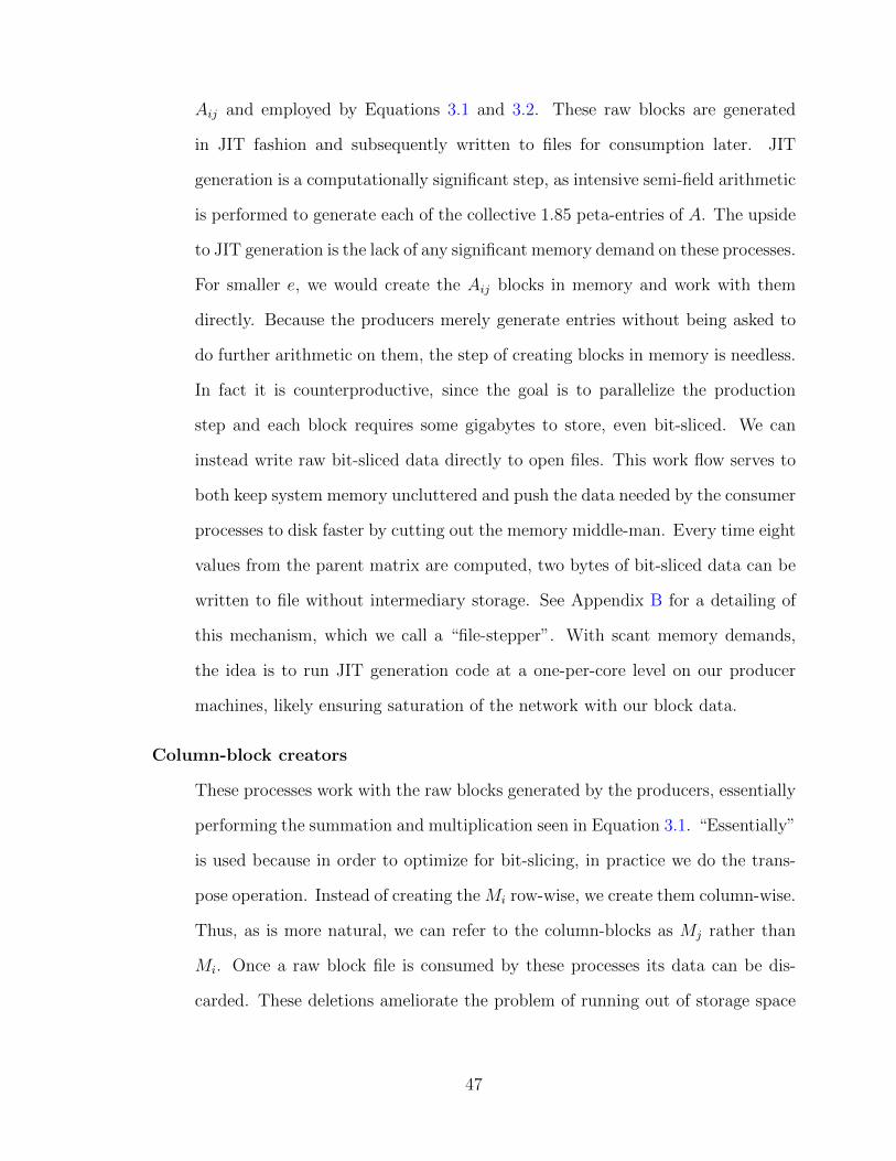
Aij and employed by Equations 3.1 and 3.2. These raw blocks are generated

in JIT fashion and subsequently written to files for consumption later. JIT

generation is a computationally significant step, as intensive semi-field arithmetic

is performed to generate each of the collective 1.85 peta-entries of A. The upside

to JIT generation is the lack of any significant memory demand on these processes.

For smaller e, we would create the Aij blocks in memory and work with them

directly. Because the producers merely generate entries without being asked to

do further arithmetic on them, the step of creating blocks in memory is needless.

In fact it is counterproductive, since the goal is to parallelize the production

step and each block requires some gigabytes to store, even bit-sliced. We can

instead write raw bit-sliced data directly to open files. This work flow serves to

both keep system memory uncluttered and push the data needed by the consumer

processes to disk faster by cutting out the memory middle-man. Every time eight

values from the parent matrix are computed, two bytes of bit-sliced data can be

written to file without intermediary storage. See Appendix B for a detailing of

this mechanism, which we call a “file-stepper”. With scant memory demands,

the idea is to run JIT generation code at a one-per-core level on our producer

machines, likely ensuring saturation of the network with our block data.

Column-block creators

These processes work with the raw blocks generated by the producers, essentially

performing the summation and multiplication seen in Equation 3.1. “Essentially”

is used because in order to optimize for bit-slicing, in practice we do the trans-

pose operation. Instead of creating the Mi row-wise, we create them column-wise.

Thus, as is more natural, we can refer to the column-blocks as Mj rather than

Mi. Once a raw block file is consumed by these processes its data can be dis-

carded. These deletions ameliorate the problem of running out of storage space

47

for A, provided the ratio of consumed to produced raw blocks is sufficiently high.

Consumer processes, unlike producer processes, are performing arithmetic on the

blocks. Despite that fact, the production step is more expensive computation-

ally, as the producers are working in the semi-field F3e while consumers take

advantage of very fast bit-slicing over F3. Thus the aforementioned ratio is in

practice high enough so that data can be incrementally deleted fast enough to

avoid overloading storage capacities.

Final-block creators

The second stage of consumption deals with the output from the first class

of consumers. These processes perform the summation and multiplication of

Equation 3.2 (technically, the equivalent transpose operation). This amounts to

combining the column blocks, Mj, into our final block M . Just as the first class

of consumers could delete the Aij after consumption, so too can this class of

consumers delete the Mj after they have been incorporated into M . This is not

quite as large an issue as j is bounded by nb

whereas there are (nb)2 raw blocks

to generate. Still, using the 5 gigabytes-per-block number from Section 3.3.2,

the Mj if combined would occupy over 1.4 TB. While we could account for this

particular amount of data, the code is robust enough to handle deleting the Mj.

This would be useful in computing, say, D(3, 9). When this stage is complete,

we can then compute rank(M). If this rank is certified by our heuristic given in

Section 3.2.2, with high probability rank(M) = rank(A).

3.3.3.1 Broad implementation

With the extra tier of consumers, this distributed layout is slightly more complex

than a canonical producer/consumer model. Even so, this division of labor fits well

within the master/slave parallel programming paradigm, an example of which is given

by Gropp et al. in [30]. Under this paradigm a central master process oversees, divides,

48

and delegates the necessary work to (typically many) distributed slave processes. Of

the diverse set of parallel programming approaches, two main archetypes come to

mind for accomplishing master/slave parallelism: remote procedure calls (RPC) and

message passing. For a variety of reasons, we chose to employ RPC for inter-process

communication, specifically via the Python Remote Objects (PyRO) module. RPC

solutions typically operate at a higher level of abstraction than message passing does

(in fact, RPC may employ message passing). Therefore, RPC-based programs are often

less complicated to write and administer. This fact — combined with the choice of an

interpreted, cross-platform language such as Python — enabled rapid prototyping and

deployment of our management system.

The diverse set of target machines and heterogeneity of our groups of processes

both also played a role in this decision. PyRO allows workers to communicate with

a central host by essentially making a TCP connection to it. Message passing on

the other hand, would involve a non-trivial amount of additional set-up costs. Such

costs would include administering a compatible message passing standard (such as

MPI, for example) between the wide array of candidate worker machines. Certainly,

not electing for message passing foregoes a certain degree of flexibility and generally

advanced features. However we have to consider our use-case. We require no more

than maintaining shared work queues; this is one of the simplest possible methods of

task delegation.

RPC, plainly speaking, allows hosts across a shared network to access remote

procedures, or program functions, and call them as if they were local. PyRO extends

this concept to an object-oriented programming model by allowing for, as the acronym

suggests, remote objects. For the reader uninitiated with the Python programming

language, everything (class, method, function, even each basic type) is an object. An

object in classical parlance means something that encapsulates data via attributes

and act on that data via methods. In Python, as in many languages, an object can

always be assigned to a variable and passed as an argument to a function. A class is

the standard programming concept used to define an object. The basic strategy is to

49

Figure 3.2: Decomposition and compression of the matrix A. Represented verticallyis the result of performing Equation 3.1 to create the Mj column-blocks(represented as a darker version of their lighter-colored Aij components.These are combined into the final block, represented by the horizontalflow of data at bottom. This represents the action of Equation 3.2.

create a class to carefully manage work queues, then instantiate an object from this

class to share between the slaves.

Following are some loose method sketches, presented directly in Python code (or

comments) rather than in pseudo-code. Python, which uses indentation rather than

character delimiters to logically group code, reads enough like pseudo-code that further

abstraction is unnecessary. That said, a brief illumination of some Python details is in

order:

• the import keyword is used to make use of external Python modules (loadablecode). In the following fragments, we will import some modules from Python’sstandard library (code distributed with Python itself) as well as some custommodules.

50

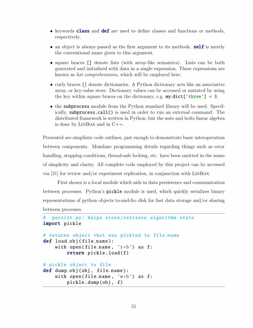
• keywords class and def are used to define classes and functions or methods,respectively.

• an object is always passed as the first argument to its methods. self is merelythe conventional name given to this argument.

• square braces [] denote lists (with array-like semantics). Lists can be bothgenerated and initialized with data in a single expression. These expressions areknown as list comprehensions, which will be employed here.

• curly braces {} denote dictionaries. A Python dictionary acts like an associativearray, or key-value store. Dictionary values can be accessed or mutated by usingthe key within square braces on the dictionary, e.g. my dict[’three’] = 3.

• the subprocess module from the Python standard library will be used. Specif-ically, subprocess.call() is used in order to run an external command. Thedistributed framework is written in Python, but the nuts and bolts linear algebrais done by LinBox and in C++.

Presented are simplistic code outlines, just enough to demonstrate basic interoperation

between components. Mundane programming details regarding things such as error

handling, stopping conditions, thread-safe locking, etc. have been omitted in the name

of simplicity and clarity. All complete code employed by this project can be accessed

via [31] for review and/or experiment replication, in conjunction with LinBox.

First shown is a local module which aids in data persistence and communication

between processes. Python’s pickle module is used, which quickly serializes binary

representations of python objects to-and-fro disk for fast data storage and/or sharing

between processes.

# persist.py: helps store/retrieve algorithm stateimport pickle

# returns object that was pickled to file namedef load obj(file name):

with open(file name , ’r+b’) as f:return pickle.load(f)

# pickle object to filedef dump obj(obj, file name):

with open(file name , ’w+b’) as f:pickle.dump(obj, f)

51

These functions are modularized to reduce code repetition and more easily share

them between the following scripts, many of which will require this functionality. With-

out further ado, the bare-bones sketch of the single shared object that controls the flow

of the algorithm:

from Queue import Queuefrom persist import load obj , dump obj

class BlockManager():def init (self):

self.work out = Queue()self.work in = Queue()

# queue each block for productionfor i in range(0, n, b):

for j in range(0, n, b):block = (i,j)self.work out.put(block)

# methods for remote invocation:def get work(self):

return self.work out.get()

def work done(self, block):self.work in.put(block)

def get produced block(self):return self.work in.get()

def consumed block(self, block):#if all blocks in a column have been created:j = block[1]created = load obj("created.dict")created[j] = Truedump obj(created, "created.dict")

PyRO allows us to distribute this master object to any machine that can aid

in computation, to process work acquired from the queues. See Appendix A for more

details on how this object is made available for RPC. This object will be referenced as

the variable manager in the remotely-run worker scripts.

52

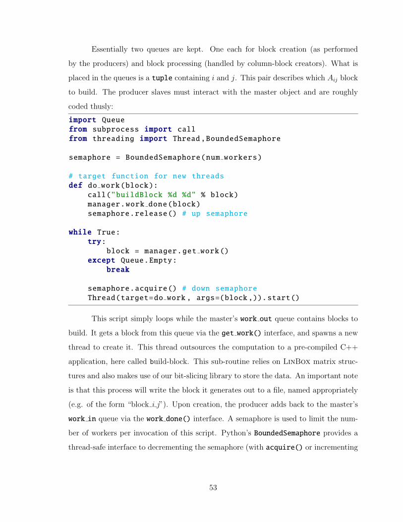
Essentially two queues are kept. One each for block creation (as performed

by the producers) and block processing (handled by column-block creators). What is

placed in the queues is a tuple containing i and j. This pair describes which Aij block

to build. The producer slaves must interact with the master object and are roughly

coded thusly:

import Queuefrom subprocess import callfrom threading import Thread,BoundedSemaphore

semaphore = BoundedSemaphore(num workers)

# target function for new threadsdef do work(block):

call("buildBlock %d %d" % block)manager.work done(block)semaphore.release() # up semaphore

while True:try:

block = manager.get work()except Queue.Empty:

break

semaphore.acquire() # down semaphoreThread(target=do work , args=(block ,)).start()

This script simply loops while the master’s work out queue contains blocks to

build. It gets a block from this queue via the get work() interface, and spawns a new

thread to create it. This thread outsources the computation to a pre-compiled C++

application, here called build-block. This sub-routine relies on LinBox matrix struc-

tures and also makes use of our bit-slicing library to store the data. An important note

is that this process will write the block it generates out to a file, named appropriately

(e.g. of the form “block i j”). Upon creation, the producer adds back to the master’s

work in queue via the work done() interface. A semaphore is used to limit the num-

ber of workers per invocation of this script. Python’s BoundedSemaphore provides a

thread-safe interface to decrementing the semaphore (with acquire() or incrementing

53

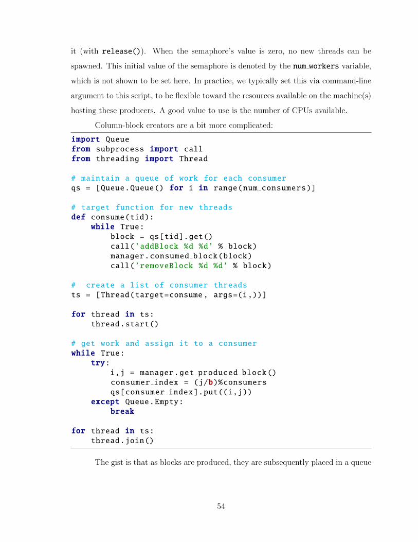
it (with release()). When the semaphore’s value is zero, no new threads can be

spawned. This initial value of the semaphore is denoted by the num workers variable,

which is not shown to be set here. In practice, we typically set this via command-line

argument to this script, to be flexible toward the resources available on the machine(s)

hosting these producers. A good value to use is the number of CPUs available.

Column-block creators are a bit more complicated:

import Queuefrom subprocess import callfrom threading import Thread

# maintain a queue of work for each consumerqs = [Queue.Queue() for i in range(num consumers)]

# target function for new threadsdef consume(tid):

while True:block = qs[tid].get()call(’addBlock %d %d’ % block)manager.consumed block(block)call(’removeBlock %d %d’ % block)

# create a list of consumer threadsts = [Thread(target=consume, args=(i,))]

for thread in ts:thread.start()

# get work and assign it to a consumerwhile True:

try:i,j = manager.get produced block()consumer index = (j/b)%consumersqs[consumer index].put((i,j))

except Queue.Empty:break

for thread in ts:thread.join()

The gist is that as blocks are produced, they are subsequently placed in a queue

54

such that get produced block() will return them. This indicates to the consumers

that a new block exists and is ready to be incorporated into a column-block. This step

is again delegated to a pre-compiled C++/LinBox program, here called addBlock.

addBlock, in short, reads in a column-block from file (representing Mj and initialized

to the zero-matrix) then reads in the new block, also from file. It adds the two blocks

together, as well as left-multiplies the new block by the appropriate Ui to obtain its

random linear contribution to the strip of rank-certifying rows along the bottom of

the column-block. After doing this, the column-block is written back to its file. This

means we do not want more than one consumer contributing to the same column block

at any one time. If there were multiple column-block creators attempting to work in

the same column, they could end up overwriting the work of one another. Therefore,

a locking mechanism would need to be designed. Code spending time waiting for a

lock on a file to open is precious concurrency wasted. In order to keep processors

saturated with work, the simplest solution is to restrict individual threads to work on

their own column-blocks. In the code, this is accomplished by creating a child-queue

per each intermediate consumer. When a signal is received of a freshly-written raw

block, the code does a division (with remainder) to determine which thread “owns” the

column-block to which the raw block belongs. Each thread checks its own child-queue,

performs any work, and informs the master process that the block has been consumed.

Most importantly, after a successful block consumption, the block is deleted to free up

disk space (by routine removeBlock). To reiterate, this step is necessary as we lack the

physical resources to store every block simultaneously. As with the producers, a special

variable is used (num consumers) to determine how many jobs will run in parallel.

So, the column-blocks (Mj) are created. The final step is to combine these to

form the final matrix M . In this first iteration of design, there is only one final-block

creator. The completion of a column-block is infrequent enough such that combinations

of the blocks can be done sequentially without much opportunity for overlapping work

(i.e. potential parallelism). Thus, there is no third queue informing the final-block

creator when column blocks are ready. Instead, it can afford to loop indefinitely,

55

checking for the existence of new column-blocks on the fly. The final structure ends up

looking like this:

from subprocess import callfrom persist import load obj , dump obj

consumed = load obj("consumed.dict")

while True:created = load obj("created.dict")

# loop over every possible column−of−blocksfor j in range(0, n, b):

if created[j]:if not consumed[j]:

call("addColBlock %d" % j)consumed[j] = Truecall("removeColBlock %d" % j)dump obj(consumed , "consumed.dict")

Here, we use our persistence module to use and maintain two Python dictionar-

ies. Both dictionaries detail the state of column-blocks: one to keep track of those that

have been created, and another to keep track of those consumed. The keys are the

column numbers, and the values are simple booleans. The dictionary of created column-

blocks is maintained by the consumed block() method of our central BlockManager

object. Under this design, this final consumer can simply loop over each column index.

If a column-block is encountered that has been created but not yet consumed, then the

consumer incorporates it into the final block with addColBlock, thus consuming it.

Then, the consumer marks the column off in the “consumed” dictionary, checkpointing

the results to disk. Again, as with the first tier of consumer, we delete the data which

we have just read and processed to free up room for further blocks to be created.

These four simple scripts unify the three stages of work by a central man-

ager. Any machine where we can compile the basic C++ components, buildBlock,

addBlock, and addColBlock, we can use in the framework of the algorithm (provided

also that they also have access to the networked file system where we store the blocks

(Aij), column-blocks (Mj), and master-block (M). In addition to ease-of-deployment,

56

we created some additional design goals. Communication both asynchronous and mod-

ular is desirable — we want to be able to pause our computation and add or remove

contributing slave processes as shared resource availability fluctuates. Asynchronous

communication also makes fault tolerance an easier proposition. Given how large and

long-running this task is, a design goal is to be able to checkpoint algorithm progress

so that recovery from error is feasible, be it a single failed job or a more widespread

ill (such as a system failure or power outage). This is doubly true when considering

how much data is necessarily generated and discarded for this job. In addition to CPU

time, disk and network bandwidth are shared, finite resources. Designing a framework

to minimize duplication of effort is crucial.

Already briefly discussed was a dictionary-pickling mechanic, which kept track

of which column-blocks had been produced, and also finally incorporated into the

master-block. In addition to providing enough communication to the final-block creator

process, this also serves as a fingerprint of the current algorithm’s progress. If a column

block has been marked as produced, the basic blocks from which it is composed would

not need to be computed were some condition encountered that required restarting

computation. This feature has been extended to keeping track of which Aij have been

combined into the column-blocks themselves, to eliminate the need for their potential

regeneration. Another concern is a potential loss of power during a file-write operation.

Remember, we are dealing with writing blocks stored in files that exceed 5 gigabytes,

even when writing raw bit-sliced data. It does not matter what modifications are made

to the code, disks have a physical write-speed limit. These files will take plenty of time

to read and write. For this reason, any time a file being is written which will be read

again as input later, it will be written to a temporary file. In this algorithm, column-

block files and the master-block file qualify for this treatment. Upon completion of

the write-to-temporary, the temporary file can be safely used as the up-to-date file for

future reads, and the appropriate dictionary-checkpoint can be registered.

57

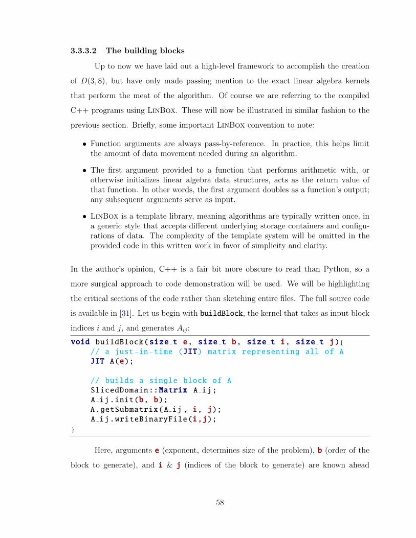
3.3.3.2 The building blocks

Up to now we have laid out a high-level framework to accomplish the creation

of D(3, 8), but have only made passing mention to the exact linear algebra kernels

that perform the meat of the algorithm. Of course we are referring to the compiled

C++ programs using LinBox. These will now be illustrated in similar fashion to the

previous section. Briefly, some important LinBox convention to note:

• Function arguments are always pass-by-reference. In practice, this helps limitthe amount of data movement needed during an algorithm.

• The first argument provided to a function that performs arithmetic with, orotherwise initializes linear algebra data structures, acts as the return value ofthat function. In other words, the first argument doubles as a function’s output;any subsequent arguments serve as input.

• LinBox is a template library, meaning algorithms are typically written once, ina generic style that accepts different underlying storage containers and configu-rations of data. The complexity of the template system will be omitted in theprovided code in this written work in favor of simplicity and clarity.

In the author’s opinion, C++ is a fair bit more obscure to read than Python, so a

more surgical approach to code demonstration will be used. We will be highlighting

the critical sections of the code rather than sketching entire files. The full source code

is available in [31]. Let us begin with buildBlock, the kernel that takes as input block

indices i and j, and generates Aij:

void buildBlock(size t e, size t b, size t i, size t j) {// a just−in−time (JIT) matrix representing all of AJIT A(e);

// builds a single block of ASlicedDomain::Matrix A ij;A ij.init(b, b);A.getSubmatrix(A ij , i, j);A ij.writeBinaryFile(i,j);

}

Here, arguments e (exponent, determines size of the problem), b (order of the

block to generate), and i & j (indices of the block to generate) are known ahead

58

of time. As mentioned, the entries comprising the parent matrix A are determined

by formula in a semifield K × K where K is F3e . Recall the formula as provided in

Section 3.2.2.

Di,j =

−1(mod p), if i = j,

1, if i 6= j and i− j is a square,

0, otherwise.

Our JIT object performs this arithmetic and can provide arbitrary windows into this

matrix. Obtaining submatrices, here called blocks, in this fashion is a common routine

for this and other codes used in this computation. Here, we create a compressed matrix

(our SlicedDomain class encapsulates working with matrices that are bit-sliced) and

initialize it to its proper size with init(). Then we simply fill our matrix with the

data and write it to disk. A helper function writeBinaryFile() is used to write out

the data to the file name that a consuming process expects. In practice, we opt to

write to disk directly within the call to getSubmatrix() through a mechanism that

can write bit-sliced data just as soon as a sliced unit has been filled. See Appendix B

for a brief outline of said mechanism, which we call a “file-stepper”.

It is the addBlock routine that uses these raw block files:

void addBlock(size t b, size t c, size t i, size t j) {typedef SlicedDomain::Matrix Matrix;SlicedDomain MD; // provides GF(3) matrix arithmetic

// M j is the column−block under construction.Matrix M j;M j.init(b + c, b);

// Read in current stateM j.readBinaryFile(j);

// A ij is the raw−block to processMatrix A ij;A ij.init(b, b);A ij.readBinaryFile(i, j);

59

// U i is our random strip matrixMatrix U i;U i.init(c, b);MD.random(U i);

// Divide B j into its two partsMatrix M j Sum , M j Cert;M j Sum.submatrix(M j , 0, 0, b, b);M j Cert.submatrix(M j , b, 0, c, b);// incorporate A ijMD.addin(M j Sum , A ij);MD.axpyin(M j Cert , U i , A ij);

// Write new state backM j.writeBinaryFile(j);

}

We have some familiar arguments in this snippet joined by a new one, c, which

represents the number of certification rows we wish to use. This ends up serving

as the row height of our random Ui matrices and consequently the product of our

certification rows, UiAij, which pad the bottom of the Mj block we are building. The

calls to readBinaryFile() will read the appropriate block into program memory from

file, given a consistent underlying file-naming scheme. Notice the signature for our

extensively used Matrix.submatrix() function. The first argument is the matrix

that the calling object wishes to refer to (i.e. the parent matrix). The next two

arguments are the indices within the parent matrix containing the top-leftmost element

of the submatrix. In other words, these integers represent the starting corner of the

submatrix in the parent. The final pair of integer arguments represent the height and

width of the submatrix, respectively.

The matrix arithmetic is all performed via the calls to addin() and axpyin().

The axpyin() call made within this phase is fast. This mul-add operation needs to

uncompress the left matrix (i.e. extract singleton elements from a bit-sliced compressed

block). We discussed in Chapter 2 that while bit-sliced arithmetic is fast, retrieving

raw elements from bit-sliced data is computationally costly. Here, the Ui on the left are

60

comparatively small matrices, therefore so is the penalty for extracting the bit-sliced

elements.

The core, compiled application at the heart of the final-block consumer reads

very similarly:

void addColBlock(size t b, size t c, size t j) {size t m = b + c;

// M is the final−block we are buildingMatrix M;M.init(m,m);

// Read in current stateM.readBinaryFile();

// M j is the j−th column blockMatrix M j;M j.init(m,b);M j.readBinaryFile(j);

// V j is the random wide vector stripMatrix V j;V j.init(b,c);MD.random(V j);

// Divide M into its two parts, then incorporate M jMatrix M Sum k , M CertCols;M Sum k.submatrix(M, 0, 0, m, b);M CertCols.submatrix(M, 0, b, m, c);MD.addin(M Sum k , M j);MD.axpyin(M CertCols , M j , V j);

// Write new state backM.writeBinaryFile();

}

Here we introduce a variable, m, which is simply b + c. This shorthand makes

it easy to reference the final block size, which is m × m. A key difference is that

our call to axpyin() in this stage takes much longer than the previous phase. As

before, both multiplicands are compressed with bit-slicing. However in this case the

61

left multiplicand– that which is to be extracted entry-by-entry– is m× b. Fortunately,

this kernel need only be performed once per column block (nb

times in total).

3.3.3.3 A failure

The framework outlined above was tested and found to work for generating

compressed blocks which maintained original rank for D(3, e), e < 8. In theory it

could also be used to eventually generate D(3, 8). In practice, it was not successful

given our usage of the framework. To analyze why, let’s begin by loosely crunching

some numbers. Our test machine is the Chimera supercomputer at the University of

Delaware. This energy-efficient machine contains compute nodes containing 4 AMD

Opteron 6164HE 12-core 1.7GHz CPUs, for a total of 48 cores-per-node total. On this

machine, a single Aij block could be generated in about two minutes and added into its

Mj column-block in about five minutes. Remember, these tasks are being performed

independently and thus can be performed simultaneously. Therefore the total time we

can expect the algorithm to take is roughly the number of blocks multiplied by five

minutes, divided by the number of mid-level consumer processes we devote to the run.

The number of blocks is known, it is (nb

)2. Sequentially (number of block creators

= 1), this would take nearly 300 days. Fortunately, or so it would seem, parallelism

would work in our favor: devote enough processes to this task and, so long as you can

keep the work queue occupied, have your block built after a couple of weeks.

Therein lied the faulty assumption. Recall from the code outlines in the previous

section the calls to readBinaryFile() and writeBinaryFile(). Communication

between the groups of processes is entirely file-based. A central file-server is used to

share files to processes running on separate hardware. As it turned out, the amount

of parallelism desired out of the mid-level column-block producers was too large a

burden on the combination of network and disk. Preventing the supply of Aij blocks

from running out meant producing at least one such block per consumer every five

minutes. This is not even accounting for the top-tier of consumers, which of course use

the file space as well to read and write their own data, albeit less frequently. Having

62

Figure 3.3: Filesystem activity during parallel build of D(3, 8). Green line is readbandwidth and blue line is write bandwidth. Bandwidth is measured inMB/sec and plotted every 5 seconds.

multiple processes constantly reading and writing files on the order of gigabytes to the

same networked file-system was simply not scalable. Such over-activity would prove

too much for our file server, which would on occasion even drop network link in the

middle of our operations, rendering our code unable to continue at all. Scaling back

the amount of parallelism was an option that would eventually lead to success, but

with only a few processes working, we would still be waiting months on end to simply

build our compressed block M , to say nothing of computing its rank.

Figure 3.3 demonstrates the utter chaos endured by the networked file system

during our attempted runs. Witness the disk frantically trying to keep up with the

sheer volume of simultaneous write requests. Under these conditions, column-block

creator processes would take tens of minutes, even over an hour, to complete their task

which under ideal conditions would only take five minutes. Blocks were being built in

memory quickly but written to disk slowly.

Practical failings aside, another limitation of the first decomposition of labor

63

is that there can only exist a single group of each type of process (producer and

consumers). Without intensive micromanagement (which would break a previously

stated design goal) multiple groups of column-block creators could trample each other’s

work. It is clear that a different approach is necessary, one that learns from the failures

of our first attempt.

3.3.4 Producer/consumer: cut out the middle-man

Writing each Aij block to a file to be consumed by another process turned out

to be a needless endeavor. One of the side goals in initially deciding on that model

had to do with testing the installation of a new 10-Gigabit Ethernet backbone at the

University of Delaware. Our ability to quickly generate useful, non-synthetic data

was only limited by the amount of processing power we had available. Therefore our

algorithm, as originally written, was an excellent candidate to test the operation of

the new link between buildings on campus, in cooperation with Central IT services.

The idea was to employ machines from various buildings each generating Aij blocks

and write them to files accessed remotely over the new link. The network handled the

data with aplomb, but the single point of failure was the workhorse file-server that

simply could not keep up with such load. Network properly tested, but algorithmic

goals unmet, the following simplified decomposition was devised.

Producers (column-block creators)

The bottom two tiers of parallelism from the failed labor-decomposition have been

merged together. Producer processes are now tasked with generating column-

blocks of A, called Mj. The JIT procedure for generating raw Aij blocks is the

same as before. Instead of being the end goal, the JIT procedure is used as a

kernel of this new process, which no longer bothers to write intermediate blocks

to memory. This means producers will now be (significantly) longer running,

but keeping the Aij in memory as opposed to writing them to disk, is much less

burdensome on the hardware. Unlike before, these producers will now have some

64

memory demand, approximately 10 GB worth: 5 for the raw-block being calcu-

lated at any given time, and another 5 for the column block ultimately being

produced. Such demand is not unreasonable on modern hardware. These pro-

ducers will avoid saturating the disk controller with writes while the consumers

are reading data.

Final-block creators

This class of processes is identical to the highest-tier of parallelism from the pre-

vious iteration (see p. 48). Briefly, again, these processes perform the summation

and multiplication of Equation 3.2.

3.3.4.1 Revised big-picture layout

As before, a central communication hub is used to coordinate efforts of the slave

processes. The low level details (PyRO RPC model) are all the same, but the high-level

operations have changed slightly. Of course, only dealing with two categories of slaves

makes things simpler:

from Queue import Queuefrom persist import load obj , dump obj

class ColBlockManager():def init (self):

self.created = load obj("created.dict")self.work out = Queue()# queue each column−bloc for productionfor j in range(0, n, b):

self.work out.put(j)

# methods for remote invocation:def get work(self):

return self.work out.get()

def work done(self, col):self.created[j] = Truedump obj(self.created, "created.dict")

65

Only one queue is now kept. This time, it is for column-block creation (as

performed by the producers). Instead of an (i, j) tuple, integers are passed via the

queue denoting which column was produced/consumed.

The producers have changed, but not much:

import Queuefrom subprocess import callfrom threading import Thread,BoundedSemaphore

semaphore = BoundedSemaphore(num workers)

# target function for new threadsdef do work(col):

call("buildCol %d" % col)manager.work done(col)semaphore.release() # up semaphore

while True:try:

col = manager.get work()except Queue.Empty:

break

semaphore.acquire() # down semaphoreThread(target=do work , args=(col,)).start()

Rather than accepting which block to build, it accepts the aforementioned in-

teger as signal for which Mj column-block to generate. Queue input/output works

exactly as described before. This time, our thread’s pre-compiled C++ heavy-lifter is

called buildCol. Once again, this application relies on bit-slicing and LinBox. We

will again write column-block output to a conventionally-named file (containing the

column number), but less frequently. There are now exactly nb

producers required to

fully build our block M , whereas the prior method called for (nb)2 writes.

With no intermediary consumer, this leaves discussion of the column-block con-

sumers (which are the final-block producers). Their purpose mirrors the final-block

creator (2nd consumption stage) of the prior parallel layout. Rather than a single pro-

cess, however, these consumers are implemented with more parallelism in mind. In this

66

second iteration of design, there can be multiple consumers or final-block creators, each

writing output to their own matrix. At algorithm’s end, these independent matrices

can be added together to form the final block M . More on this point shortly. Once

again, the consumption phase can afford to loop indefinitely, checking for the existence

of new column-blocks. When a new column-block has been generated, it is queued for

consumption by one of the worker threads. Here is the full listing:

from subprocess import callfrom Queue import Queuefrom threading import Threadfrom persist import load obj , dump obj

ready queue = Queue()consumed = load dict("consumed.dict")

# target function for new threadsdef consume(tid):

# continuously check for new column blocks to combinewhile True:

j = ready queue.get()if j is None:

breakcall("addColBlock %d %d" % (j, tid))consumed[j] = Truecall("rmColBlock %d" % j)dump obj(consumed , "consumed.dict")

while True:created = load dict("created.dict")queued = consumed.copy()

# create the parallel workersthreads = [Thread(target=combine, args=(i,))

for i in range(num workers)]# spawn themfor t in threads:

t.start()

# loop over every possible column−of−blocksfor j in range(0, n, b):

if created[j]:if not queued[j]:

67

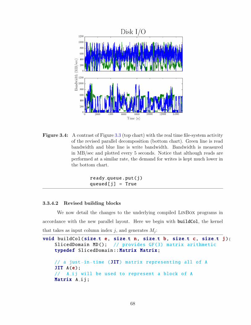
Figure 3.4: A contrast of Figure 3.3 (top chart) with the real time file-system activityof the revised parallel decomposition (bottom chart). Green line is readbandwidth and blue line is write bandwidth. Bandwidth is measuredin MB/sec and plotted every 5 seconds. Notice that although reads areperformed at a similar rate, the demand for writes is kept much lower inthe bottom chart.

ready queue.put(j)queued[j] = True

3.3.4.2 Revised building blocks

We now detail the changes to the underlying compiled LinBox programs in

accordance with the new parallel layout. Here we begin with buildCol, the kernel

that takes as input column index j, and generates Mj:

void buildCol(size t e, size t n, size t b, size t c, size t j) {SlicedDomain MD(); // provides GF(3) matrix arithmetictypedef SlicedDomain::Matrix Matrix;

// a just−in−time (JIT) matrix representing all of AJIT A(e);// A ij will be used to represent a block of AMatrix A ij;

68

A ij.init(b, b);

// M j is the column−block under construction.Matrix M j;M j.init(b + c, b);// Divide it into two partsMatrix M j Sum , M j Cert;M j Sum.submatrix(M j , 0, 0, b, b);M j Cert.submatrix(M j , b, 0, c, b);

// U i is our random strip matrixMatrix U i;U i.init(c, b);

// For each block in this column, row−wisefor(size t i = 0; i < n: i += b) {

// Retrieve the blockA.getSubmatrix(A ij , i, j);

// incorporate blockMD.addin(M j Sum , A ij);kMD.random(U i);MD.axpyin(M j Cert , U i , A ij);

}

// Write block to fileM j.writeBinaryFile(j);

}

Naturally this is just an amalgamation of the producer and the first consumer

from before. Once again, the important point is that there are no intermediate file

writes.

The addColBlock routine is unchanged from the listing given in 3.3.3.2, save one

detail. In this computational layout the consumer is written to take advantage of mul-

tiple worker threads, each of which could be consuming a column block simultaneously.

Of course, this means the threads would be adding to a master block simultaneously.

Such a mechanism is thread-unsafe. Workers could overwrite each other’s partial work,

leaving the master block in an unknown (but almost certainly meaningless) state. So

69

in practice, each thread has its own master block to write to, and this is subtly dis-

tinguished by having the call to addColBlock take as input the thread identification

number. As long as each thread used in this stage of the parallelism has a unique

identification number, no thread-collisions can occur at the file level.

Thus we are left with the following construction. If there are w workers devoted

to column-block consumption, there will be w sums of column-blocks, call them the

Mw. Let the set J be the set of all columns-of-blocks needed by the algorithm, denoted

by that column’s leftmost column index of A. Let the set Jw be the set of all columns

incorporated into Mw by a worker w, denoted the same way. The Jw are mutually

disjoint partitions of the set J . For any pair Jx and Jy, Jx∩Jy = {}. In other words,

no two workers will combine the same column-block into their private sum-block Mw.

Then,

J = {ib : 0 ≤ i <n

b}

J =⋃Jw

Therefore,

Mw =∑Jw

MJw |MJwVJw

M =∑

Mw

So, our final block M can be created by a basic summing of the intermediary

column-block sums produced by each worker. This is a quite fast operation with bit-

sliced matrices, and has negligible effect on overall running time.

3.3.4.3 Shared-memory parallelism

As mentioned, our main compute nodes had four 12-core CPUs, so taking ad-

vantage of the available shared-memory parallelism is paramount. For this feature we

turned to the ready-made OpenMP [32] framework. OpenMP is a portable, flexible

70

API for using shared memory parallelism from within C++ (among other languages)

via simple directives. For example, a revamped buildCol routine to take advantage

of OpenMP parallelism:

#include <omp.h>

void buildCol(size t e, size t n, size t b, size t c, size t j) {... // set up matrices as before

// Submatrices employed per−threadDomain::Matrix sub, msub;

// For each block in this column, row−wisefor(size t i = 0; i < n: i += b) {

#pragma omp parallel private(tid, rpt, sub, msub) shared(nthreads){

tid = omp get thread num();nthreads = omp get num threads();

rpt = b / nthreads; // rpt = Rows Per Thread

// Retrieve the sub−block for this threadsub.submatrix(A ij , rpt ∗ tid, 0, rpt, b);A.getSubmatrix(sub, i+rpt ∗ tid, j);

// add in sub−block to correct slab of M jmsub.submatrix(M j Sum , rpt ∗ tid, 0, rpt, b);MD.addin(msub, sub);

}

MD.random(U i);MD.axpyin(M j Cert , U i , A ij);

}

... // write file as before}

Set-up and tear-down have been omitted as they are unchanged from the listing

on page 68. The internal loop has been re-written to take advantage of multi-core

71

processing. The #pragma omp parallel directive will automatically separate its con-

taining “for” loop into equal chunks for separate threads to tackle. The private()

and shared() clauses indicate which variables are to be shared among all threads, and

which variables should be copied to thread-local memory for individual usage. Once

again our oft-used submatrix archetype is used. In this modification it is doubly use-

ful: a sub-matrix called sub is created by each thread which can be used to generate

entries from Aij, and another submatrix called msub is used to reference the appropri-

ate slice of the column-block, Mj to which the thread can simply add sub. The Aij

generation can be done entirely independently, meaning each thread can proceed as if

it were its own process, entirely ignorant of the work of the other threads. Of course,

the step that cannot be parallelized so simply is the call to axpyin(), which is left

outside of the OpenMP code block.

3.3.5 Obtaining rank(M)

Computing the rank of the compressed adjacency matrix of the strongly-regular

graph that we have built is the final step in our rank algorithm. Last, but not least:

calculating rank even on this vastly compressed form can still take on the order of

days with current computing resources. The algorithm we use is essentially canonical

Gaussian Elimination [17], one of the same methods that was not viable to use on the

uncompressed adjacency matrix. However, a few key improvements make this com-

putation faster. We perform a special bit-sliced and multithreaded implementation of

Gaussian elimination. Performing Gaussian elimination means converting the matrix

to row-echelon form. In this form, the nonzero rows precede the zero rows and the

number of nonzero rows is the rank of the matrix. The leading entries in the nonzero

rows are called the pivots; the columns of the pivots are in increasing order. The

exact details are not so important, but the algorithm relies on two subroutines: swap-

ping rows and vector-axpy. Swapping memory is easy enough, but bit-slicing makes

it significantly faster as every word-swap exchanges many values instead of just one.

Vector-axpy is of course also improved by virtue of the data being bit-sliced, but even

72

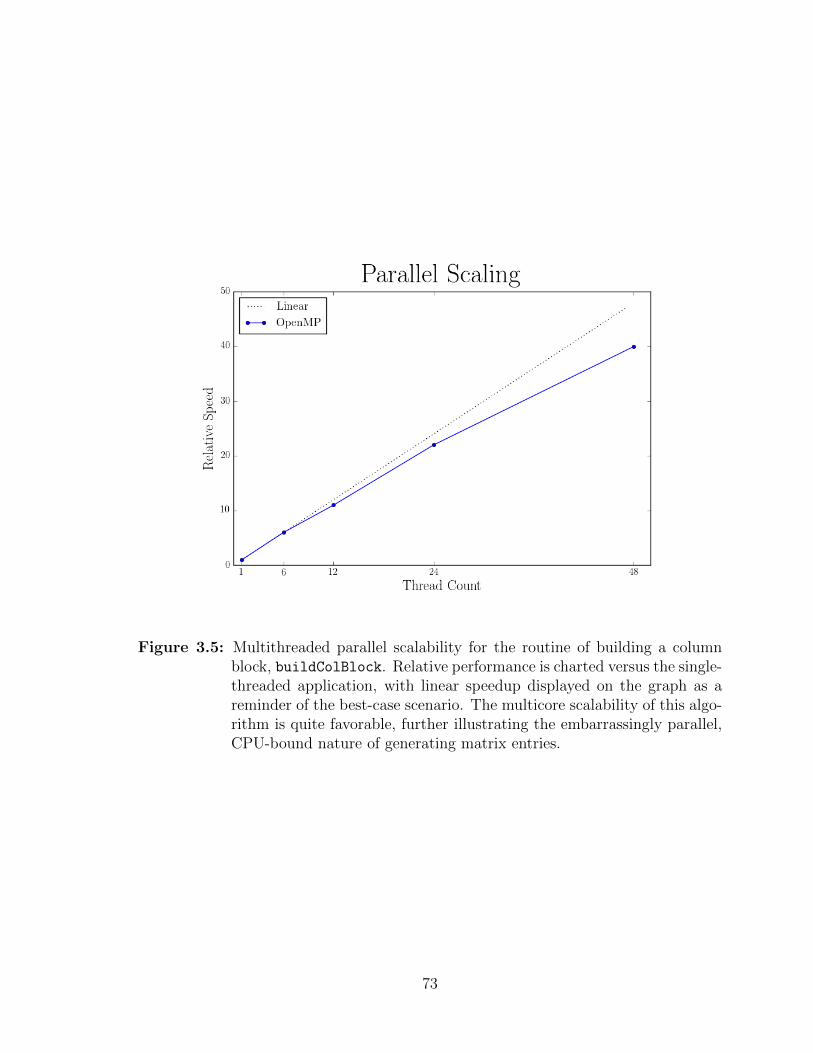
Figure 3.5: Multithreaded parallel scalability for the routine of building a columnblock, buildColBlock. Relative performance is charted versus the single-threaded application, with linear speedup displayed on the graph as areminder of the best-case scenario. The multicore scalability of this algo-rithm is quite favorable, further illustrating the embarrassingly parallel,CPU-bound nature of generating matrix entries.

73

more time is saved by again resorting to shared-memory parallelism. Each time a pivot

is found, elimination (by way of axpy) must be performed on all subsequent rows. This

step can be performed entirely independently on each row, yet another embarrassingly

parallel routine. Therefore these rows can be evenly pooled into t groups, where t is

the number of OpenMP threads available. Each thread then eliminates the rows for

which it is responsible. Table 3.2 repeats Table 3.1 with new data showing the marked

improvement bit-slicing and OpenMP have made on our simple Gaussian elimination

kernel, in the “2014r” column. Specifically, contrasting this with the “2009r” col-

umn shows an order of magnitude difference in computing the rank of the compressed

D(3, 7).

Full disclosure: the comparison over the years is not apples to apples. The times

reported in the 2014 columns were run on the Chimera supercomputer. The consid-

erable improvement seen in Table 3.2 between the “2009t” and “2014t” column in

computing rank(D(3, 7)), and indeed the very ability to compute rank(D(3, 8)) owes

largely to taking advantage of the parallelism afforded by the new machinery. The

“2014t” column, which describes time taken for the matrix compression, employed

eighteen Chimera compute nodes, whereas the rank calculation (“2014r” column) en-

joyed the contribution of 48 cores of a single node. Despite not being a fair comparison,

the new data still serves as a remarkable high level view on just how much runtime

savings bit-slicing and massive parallelism have earned us. With a time complexity

cubic and the matrix quadrupling in size with each successive entry, we expect an 81-

times increase in running time between levels on the table. The fact we have actually

cut running time between levels by a factor of three (96.4 hours in 2009 to 27.9 hours

in 2014) is a great success, and promising for the future of this line of computation.

3.3.6 A final barrier

With the new decomposition of work, we were able to compute final blocks M

that should have captured the rank of D(3, 8). However, our rank code performing

Gaussian elimination was “dipping” into the certification rows and columns we built

74

Table 3.2: Repetition of Table 3.1 with data added from the parallelimplementation— Running time for computing the ranks of Dickson ad-jacency matrices. The time units are ’s’ for seconds, and ’h’ for hours.

Dickson SRGe dimension Rank 2007t 2009r 2009t 2014r 2014t

2 81 20 0.021s 0.0003 0.0012s - -3 729 85 0.35s 0.003s 0.022s - -4 6,561 376 33.3s 0.046s 0.95s - -5 59,049 1654 0.5h 1.4s 0.017h - -6 531,441 7283 46.7h 80s 1.2h - -7 4,782,969 32064 - 1.2h 96.4h .13h 1.3h8 43,046,721 141168 - - - 8.71h 27.9h

into our block. In fact, the elimination was using up the entirety of this buffer, indi-

cating M was of full rank or M did not capture rank(D(3, 8)), or both. Something was

decidedly going wrong. The algorithm would have to be run, re-run, and thoroughly

examined in order to figure out the problem. In this light, the performance of the

distributed- and shared-memory parallel implementation proved vital. We could also

be thankful for the many-core architectures on which the code ran. The job could be

re-tried in days, not months.

3.3.6.1 The panacea

Where we stand here is that we have generated a compressed block that has not

captured the desired rank. We generated this block without the benefit of the butterfly

preconditioners detailed in Section 3.2.1. Butterfly preconditioners would ensure that

the true rank would be contained in the compressed block. However, re-engineering the

butterflies back into the code would be time-consuming, to say nothing of the massive

increase in algorithmic complexity and computational running time this would cause.

Remember, the butterfly matrices serve to “scramble” the matrix data, so much of the

effectiveness of the shared-memory parallelism detailed in the previous section would

be diminished due to inter-thread data dependence. Another factor to consider is that

75

the butterfly concept of permuting at the individual column-level is incongruent with

bit-slicing, our chosen matrix representation, which of course packs multiple matrix

columns together.

Instead the heuristic we rely upon, crudely adding the blocks together, has

proven ineffective on this iteration of the problem where it had hitherto succeeded.

It is likely in this instance that independent rows and columns of A are cancelling

each other out. Thus the preconditioning step, whilst clearly not necessary for the

computation of the prior ranks in the sequence, would greatly increase the likelihood

of capturing rank(D(3, 8)) within our built-block M . So the question now is how can

we approximate the scrambling effect of the butterfly preconditioners without losing

many of our current advantages? The answer to coarsely permute column-wise the Mj

column-blocks before combining them into M with our consumers. This is a desirable

solution as the coarse permutation is performed only nb

times per run. The permutation

is coarse because the Mj is not permuted by individual columns. Again, such an action

would be quite costly given that Mj is bit-sliced; each element to permute would have

to be masked and shifted out of its original sliced-unit before being shifted and masked

back into its final sliced-unit. Rather, the permutation occurs on sliced-unit boundaries.

If bit-sliced data is packed into 64-bit words, then the permutation is of 64 columns

at a time. This is one of the least invasive and intensive ways to radically change the

construction of the matrix. Yet it was entirely reasonable to attempt first, because

after all we have the certification rows and columns. As long as at least some of those

remain intact throughout the rank calculation, we can be reasonably sure that M ’s

rank is D(3, 8)’s rank. So of course the plan was to try the simplest things first to get

the rank to certify.

In practice, a random permutation generated by a Knuth shuffle [33] is per-

formed on the level of sliced-units. A Knuth shuffle is a method of randomly permut-

ing a sequence, which generates permutations uniformly random across the set of all

possible permutations, i.e. every permutation is equally likely. This turned out to

provide exactly the shifting around needed to avoid independent column cancellation.

76

After performing this step, the rank algorithm no longer “dipped” into the row or col-

umn certifiers containing random linear combinations of D(3, 8). We could once again

probabilistically trust that rank(M) = rank(A).

The result: 141168. How does that stack up with what was expected? Once

again we check by plugging the ranks of D(3, 5..7) into the conjectured recurrence

relation for comparison.

> 4 * 32064 + 2 * 7283 - 1654;

141168

At long last, we have successfully confirmed that the rank of D(3, 8) is equivalent

to the rank predicted by our formula!

3.3.7 Further applications

Accomplishing the rank computation ofD(3, 8), and thus giving further evidence

for a linear recurrence for the ranks, engendered a certain interest in exploring similarly

defined adjacency matrices of other families of strongly-regular graphs. Some graph

families of interest that were also described by Xiang et al. in [14] include the Paley

and the Cohen-Ganley series. A graph sequence of more recent interest is known as

the Ding-Yuan sequence [? ].

The convenient thing about attempting to calculate the ranks of these sequences

is the ability for code re-use from the Dickson sequence. In fact, nearly everything

about the framework for computing the Dickson ranks remains the same, from the JIT

generation step, to the parallel master-slave hierarchy and components, to the final-

block compression. There are two main differences between obtaining ranks of the

different families of matrices. Most simply is the fact that differently sized ranks are

expected in each case. This fact requires a minor tweak in determining the block size

b of the compressed block M . Remember, this block must of course be large enough

to entirely encompass the rank of the uncompressed JIT A.

The second difference is in pre-calculating a table of squares in the semifield

which defines the particular matrix class (e.g. Dickson, Cohen-Ganley, etc.). Recall

77

that the entry in the (i, j) position of the matrix is 1 if the difference i− j is a square

in this semifield. For efficiency we pre-compute a binary listing of every possible value

within the semifield. A one in the place of a semifield element denotes it is a square,

and a zero denotes that element is not a square. This way, upon computing i− j, all

that is necessary is a table-lookup to determine the matrix entry at these indices.

Given our success in pinning down a formula for the Dickson sequence, we have

been asked by these mathematicians to explore the unknown ranks on the larger end

of the scale for the other sequences. The hope here is that similar formulae can be

found, or at least upper bounds on the ranks can be proven. Furthermore, no simple

linear recurrence has emerged for the Cohen-Ganley and Ding-Yuan ranks as have been

computed thus far. Pushing on to even larger sizes is ultimately desirable– this means

computing the rank of matrices far larger than D(3, 8). For instance, DY (3, 8) (DY

for Ding-Yuan) is actually a matrix order 317.

The basic heuristic we rely on has proven unreliable in computing the larger

matrices in the Cohen-Ganley and Ding-Yuan families. Additional permutation steps

are likely needed to tackle these examples.

3.4 Summary

Chapter 2 detailed technologies that greatly benefited this rank problem, among

other small finite field applications. Chapter 3 motivated the rank problem, then at-

tacked it with a new theoretical approach. This approach parallelizes easily, and a new

parallel framework has been necessarily developed to compute rank of the larger matri-

ces of interest. The framework has been applied successfully to solve for rank(D(3, 8))

using about nine hundred cores over the course of days. Work is ongoing to adjust the

algorithm for the non-Dickson families, meaning ever-larger computations will follow.

As the asymptotic complexity indicates cubic growth, we can expect these runs to take

on the order of months with the same hardware. The end of this chapter concludes dis-

cussion on this problem. Chapter 4 turns to a completely different application falling

under the umbrella of exact linear algebra: rational linear system solving.

78

Table 3.3: Known ranks for adjacency matrices of certain strongly regular graphfamilies. The powers for the Ding-Yuan family are all one less than thepower listed, e.g. the Ding-Yuan matrix in 32 row is 3× 3, and the matrixin the 316 row is 315 × 315.

Order Paley Dickson Cohen-Ganely Ding-Yuan

32 4 4 4 234 16 20 20 836 64 85 94 4238 256 376 448 226310 1024 1654 2084 1232312 4096 7283 9652 6646314 16384 32064 44651 35862316 - 141168 - 185868

Known Formula X X ? ?

79

Chapter 4

EXACT RATIONAL LINEAR SYSTEM SOLVER

4.1 Introduction

We address the problem of solving Ax = b for a vector x ∈ Qn, given A ∈ Zm×n

and b ∈ Zm. Also, in this chapter we are concerned with dense matrices, which is to say,

matrices that do not have so many zero entries that more specialized sparse matrix

techniques should be applied. We do anticipate that the refined numeric-symbolic

iterative approach presented here will also apply effectively to sparse systems.

4.1.1 Relation to prior work

We present a method which is a refinement of the numeric-symbolic method of

Wan [34, 35]. Earlier work of Geddes and Zheng [36] showed the effectiveness of the

numeric-symbolic iteration, but used higher precision (thus higher cost) steps in the

residue computation. However, Wan’s method has had only sporadic success as de-

ployed in the field in LinBox. Here we present a new confirmed continuation method

which is quite robust and effective. In general, numerical iteration methods are in-

tended to extend the number of correct digits in the partial solution x′. The confirmed

continuation method verifies that these new digits overlap the previous iteration’s par-

tial solution. The concept of “overlap” here will be explained in detail in Section 4.3.

This is our assurance of progress, rather than the less reliable matrix condition num-

ber small norm of residual, |b − Ax′|, which is used in prior methods [34, 35, 37, 38].

Evidence from data suggests that the new version solves a larger class of problems, is

more robust, and provides the fastest solutions for many dense linear systems.

Standard non-iterative methods, such as Gaussian elimination, suffer from ex-

treme expression swell when working in exact integer or rational number arithmetic.

80

In fact, the solution vector x itself is typically a larger object than the inputs. When

elimination is used, typically O(n2) large intermediate values are typically created,

with concomitant large time and memory cost.

In view of such expression swell, it is remarkable that iterative methods provide

for solution in n3+o(1) time and n2+o(1) space when input entry lengths are constant.

(The factor no(1) absorbs any factors logarithmic in n.) There are two contending

approaches.

A classical approach for finding rational number solutions to linear systems is

Dixon’s modular method [39]. This method begins by solving the system modulo a

prime, p, and proceeds to a p-adic approximation of the solution by Hensel lifting,

and finishes with reconstruction of the rational solution from p-adic approximants of

sufficient length. The second approach is a numeric-symbolic combination introduced

by Wan in his thesis [34, 35]. Our focus is on extending Wan’s method to to a larger

class of problems where the size of residuals is too pessimistic.

The more usual iterative refinement of solutions within working floating point

precision has excellent exposition in [40]. Historically, the idea of solving exact linear

systems to arbitrarily high accuracy by numerical iterative refinement (earlier referred

to as binary-cascade iterative-refinement process, BCIR) is attributed to H. Wozni-

akowski by Wilkinson [41]. Wozniakowski is also acknowledged in a 1981 paper by

Kielbasinski [38]. This 1981 paper emphasized “using the lowest sufficient precision in

the computation of residual vectors.” The required precision was allowed to vary at

each iterative step. The case when doubling the working precision suffices to compute

sufficiently accurate residuals was also treated soon after in [37]. An important limita-

tion of these early papers was the assumption that the condition number of the matrix

A is known. In practice, the system’s condition number is rarely known and estimators

can fail drastically.

Wan introduced two innovations into iterative refinement. The first innovation

is that knowledge of condition numbers is not required. Instead, the accuracy of inter-

mediate approximation vectors is estimated by the computed residuals, |b−Ax′|. Wan’s

81

second innovation was to compute these residuals exactly, rather than in variable pre-

cision or double precision as in the two earlier papers. Accurate residuals are essential,

of course, for the correctness of subsequent iterative steps. However, residuals, even if

exact, do not always correctly assess the accuracy of approximate solutions.

Thus, Wan’s approach is basically to iterate with a series of approximate nu-

merical solutions, each contributing a possibly differing number of correct bits, and to

do exact computation of the current residual (via truncation and scaling) at each iter-

ation in preparation for the next. The exactly computed residual is used to estimate

the number of reliable bits in the current numeric approximation, and to provide the

required accuracy of the residual that is to be input into the next iterative step. The

final step in Wan’s method, just as in Dixon’s method, is that rational construction of

the exact solution is undertaken only after a sufficiently accurate (dyadic, in this case)

rational approximation is obtained.

One may say that, as input to the rational reconstruction, Dixon’s method

produces terms of a Laurent series in powers of the prime p and numeric-symbolic

iteration produces terms of a Laurent series in powers of 1/2. A bound is computed for

the maximum length of the series necessary to assure rational reconstruction. These

methods have the same asymptotic complexity.

Reconstruction earlier in the process can be tried and will succeed if the rational

numbers in the solution have smaller representations than the a priori bound. This

is not done in the current implementation of Wan’s method. Steffy studies this case

in [42]. We offer a variant of rational reconstruction which recognizes potential early

termination. But we distinguish these speculative results from the results that are

guaranteed from known properties of the output and length of the Laurent series.

Speculative results should be checked to see if they satisfy the original linear system.

One advantage of numeric-symbolic iteration is that the most significant digits

are obtained first. One can stop short of the full rational reconstruction and instead

take as output the floating point values at any desired precision. A disadvantage of

numeric-symbolic iteration is that it does require the numeric solver to obtain at least

82

a few bits of accuracy at each iteration to be able to continue. Thus it is subject to

failure due to ill-conditioning.

Wan’s method has been implemented in LinBox [43, 1]. Some uses of linear

system solving, for instance in Smith Normal Form computation, proceed by trying

Wan’s method and, if it fails, resorting to Dixon’s. Unfortunately, past experience is

that the numeric-symbolic iteration fails more often than not in this context. The con-

firmed continuation algorithm variant reported here significantly increases the success

rate.

In section 4.2, we explore Dixon’s and Wan’s iterations in more detail. Then in

section 4.3 we describe our confirmed continuation method. In section 4.4 the rational

reconstruction phase is discussed in detail. Finally our experiments are reported in

section 4.5.

4.2 Background

Here is a unified skeleton of Dixon’s p-adic method and the numeric, dyadic

iteration for rational linear system solution. To unify the notation note that a rational

number x may be written as a Laurent series: x =∑∞

i=k xipi, where either p is a prime

(p-adic expansion) or p = 1/2 (dyadic expansion). It will be convenient to think of the

dyadic expansion in e bit chunks, in other words, use p = 2−e. We specify that each

xi is integer and 0 ≤ xi < p in the p-adic case, 0 ≤ xi < 1/p in the dyadic case. In

either case let x mod pl denote∑l−1

i=k xipi. This will allow us to use the same modular

language when discussing p-adic or dyadic expansions.

The skeleton of iterative refinement schemes to compute a solution x to Ax = b

is then the following.

1. Compute B such that B = A−1 mod p. That is, A ∗ B = I mod p. The neededfunctionality of B is that for various vectors r, it can be used to accuratelycompute A−1r mod p in n2 arithmetic steps. For instance, B could be representedby an LU decomposition of A.

2. By Cramer’s rule the solution vector can be represented by quotients of n × nminors of (A, b). Compute a bound H (for instance the Hadamard bound) for

83

these determinants. Let k = dlogq(H)e, where q = p if doing p-adic expansionand q = 1/p if doing dyadic expansion. 2k terms of expansion are needed, in theworst case, to reconstruct the rational numbers in the solution vector.

3. Let r0 = b, y0 = 0. For i in 0..2k do the following:

(a) yi = A−1ri mod p.

(b) ri+1 = (ri−Ayi)/p. Do this computation modulo p2 at least. Since ri−Ayi =0 mod p, after the division, ri+1 is the correct residual modulo p.

(c) y = y + yipi.

Each of these steps corrects for the preceding residual by computing y to onemore p-adic digit of accuracy. In other words y = A−1b mod p2k.

4. Apply rational reconstruction to the pair of (y, p2k) to obtain x, the solutionvector of rational numbers.

When p is a prime, this is Dixon’s method. When p = (1/2)30 this is essentially

Wan’s numeric-symbolic iterative scheme. Wan’s method succeeds so long as step (3a)

yields at least some bits of accurate data at each iteration. Thus there is the possibility

of failure due to insufficient numeric accuracy in the iteration, a problem not present

in Dixon’s method. On the other hand, it is possible to exploit whatever amount of

accuracy is achieved at each step, which could be more or fewer than 30 bits. In other

words, there is no need to use the same power of 1/2 at each iteration. Wan’s iteration

(and others) adjust the number of bits used at each iteration to the accuracy of the

solver.

The trick to this on-line adjustment is to know the accuracy of the solver. The

condition number and/or the norm of the residual have been used as guidance here.

The residual norm idea is basically that in step (3b) if ri+1 = ri − Ayi is smaller by e

bits than ri, then also the first e bits of yi are likely to be accurate. However, this is

not always the case.

The first contribution of our approach is to replace the use of the residual norm

with an overlap confirmed continuation principle. Suppose it is believed that e bits of an

intermediate numeric solution are accurate. The residual norm based iteration would

84

define yi as w mod 2−e. Thus w = yi + 2−eq, (q ≤ 1) and q is discarded1. Instead,

we choose the exponent e′ of 1/2 used at each iteration slightly conservatively. Let

e′ = e− 1 and use the decomposition w = yi + 2−e′q. We take a little less in yi so as to

be able to make use of q. Since we believe the numeric solver gave us e bits of accuracy,

the first bit in each entry of q is presumably accurate. Thus yi+1 should agree with q in

the leading bits. When this happens we say we have a confirmed continuation. When

it fails, we recognize that w was not accurate to e bits, and make an adjustment as

described in the next section.

Confirmed continuation is a heuristic, since when it succeeds we do not know

with certainty that the solution is accurate. It will succeed very well when the numeric

solver is unbiased and the intuition is that it will still do very well when bias is present.

Let A ∈ Zn×n and let B be a representation of A−1. Suppose B is unbiased, which

means that, for any b ∈ Zn, s ∈ Z, if y = Bb mod 2s and y 6= A−1b mod s then

the direction of B(b − Ay) is uniformly random. Observe that if B is unbiased then

the probability is 1/2n of a false one bit continuation confirmation. This is just the

observation that there are 2n patterns of n bits. This is a rather weak justification for

our confirmed continuation heuristic since solvers are rarely if ever unbiased. However,

in practice the heuristic is proving to be effective, allowing continuation in some cases

in which the residual norm is discouragingly large.

In the next section our confirmed continuation method is described in more

detail including the exploitation of techniques to discover the solution sooner when

the actual numerators and denominator are smaller than the a priori bounds. This

is variously called output sensitivity or early termination [44, 45]. Output sensitivity

has been used primarily with Dixon’s algorithm. The only study of it we know for

numeric-symbolic iteration is [42].

1 It is a central idea of Wan’s approach to do this truncation so that the next residual may becomputed exactly.

85

4.3 Confirmed continuation and output sensitivity

Our variant on iterative refinement, sketched in Algorithm 15, uses the same

basic structure as previous implementations. That is, the system is solved numerically

in a loop, with the solution at each iteration contributing some bits to the dyadic nu-

merators and common denominator. Specifically, we call the solution in a step of the

iteration x, and divide it into two parts, called xint and xfrac. xint contains the higher

order bits and is incorporated into the dyadic estimate. xfrac contains the lower order

bits and is unused in Wan’s algorithm. The residual vector obtained by applying A to

xint provides the right-hand side to solve against for the next iteration. The loop ends

when it is determined the dyadic approximants contain enough information to recon-

struct the true rational solution. As mentioned in Section 4.1.1, this determination is

made by checking against a pre-computed bound on the size of the rationals.

To ensure the accuracy of the numeric solver’s solution at each iteration, we

verify that there is overlap between the current iteration’s numeric solution, x and

the discarded fractional portion of the previous solution xfrac. The two vectors are

subtracted and the maximal absolute value in the difference set is checked against a

threshold, 12k, to ensure k overlapping bits. In practice, we find one bit of overlap (i.e.

k = 1) suffices to confirm continuation except for very small n.

4.3.1 An adaptive approach

Once this verification step is successful, we are able to explore seeking more bits

of accuracy from the numeric solver. We treat the value s as an adjustable bit-shift

length. Each numeric solution x is multiplied by 2s in order to split into xint and xfrac.

That is, it is bit-shifted left by s. Likewise when we update the dyadic numerators N ,

we shift them left by s, then add the new information to the now zeroed lower s bits.

The value of s is at our disposal and allows the algorithm to adapt to changing

accuracy from the numeric solver. Ideally it will hug the true number of accurate bits

in the intermediate results as closely as possible. As long as some bits of accuracy

are provided by each numeric solve, the iteration can continue. Within the bounds

86

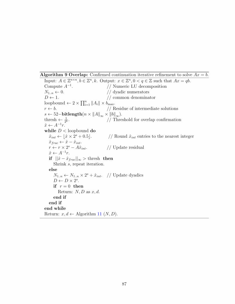
Algorithm 9 Overlap: Confirmed continuation iterative refinement to solve Ax = b.

Input: A ∈ Zn×n, b ∈ Zn, k. Output: x ∈ Zn, 0 < q ∈ Z such that Ax = qb.Compute A−1. // Numeric LU decompositionN1..n ← 0. // dyadic numeratorsD ← 1. // common denominatorloopbound ← 2×

∏ni=1 ‖Ai‖ × bmax.

r ← b. // Residue of intermediate solutionss← 52−bitlength(n× ‖A‖∞ × ‖b‖∞).thresh ← 1

2k. // Threshold for overlap confirmation

x← A−1r.while D < loopbound doxint ← bx× 2s + 0.5c. // Round xint entries to the nearest integerxfrac ← x− xint.r ← r × 2s − Axint. // Update residualx← A−1r.if ||x− xfrac||∞ > thresh then

Shrink s, repeat iteration.elseN1..n ← N1..n × 2s + xint. // Update dyadicsD ← D × 2s.if r = 0 then

Return: N,D as x, d.end if

end ifend whileReturn: x, d← Algorithm 11 (N,D).

87

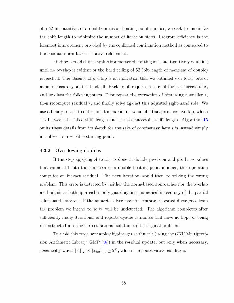
of a 52-bit mantissa of a double-precision floating point number, we seek to maximize

the shift length to minimize the number of iteration steps. Program efficiency is the

foremost improvement provided by the confirmed continuation method as compared to

the residual-norm based iterative refinement.

Finding a good shift length s is a matter of starting at 1 and iteratively doubling

until no overlap is evident or the hard ceiling of 52 (bit-length of mantissa of double)

is reached. The absence of overlap is an indication that we obtained s or fewer bits of

numeric accuracy, and to back off. Backing off requires a copy of the last successful x,

and involves the following steps. First repeat the extraction of bits using a smaller s,

then recompute residual r, and finally solve against this adjusted right-hand side. We

use a binary search to determine the maximum value of s that produces overlap, which

sits between the failed shift length and the last successful shift length. Algorithm 15

omits these details from its sketch for the sake of conciseness; here s is instead simply

initialized to a sensible starting point.

4.3.2 Overflowing doubles

If the step applying A to xint is done in double precision and produces values

that cannot fit into the mantissa of a double floating point number, this operation

computes an inexact residual. The next iteration would then be solving the wrong

problem. This error is detected by neither the norm-based approaches nor the overlap

method, since both approaches only guard against numerical inaccuracy of the partial

solutions themselves. If the numeric solver itself is accurate, repeated divergence from

the problem we intend to solve will be undetected. The algorithm completes after

sufficiently many iterations, and reports dyadic estimates that have no hope of being

reconstructed into the correct rational solution to the original problem.

To avoid this error, we employ big-integer arithmetic (using the GNU Multipreci-

sion Arithmetic Library, GMP [46]) in the residual update, but only when necessary,

specifically when ‖A‖∞ × ‖xint‖∞ ≥ 252, which is a conservative condition.

88

The matrix norm is computed beforehand, so it costs only O(n) work per iter-

ation to compute the vector norm. The flexibility of this approach both prevents the

aforementioned divergent behavior and allows for the use of quicker, double precision

computation of the exact residual in many cases. Our experience is that for borderline

problems that require some bignum residual computation, the need is rare amongst

iterations.

4.3.3 Early termination

Sometimes the numerators and denominator of the final rational solution are

significantly smaller than the worst case bound computed a priori. When this is the

case, it is possible to obtain dyadic approximants of sufficient length to reconstruct the

solution before the iterative refinement would normally end. Our early termination

strategy is designed to improve algorithmic running time in these cases. It is sketched

in Algorithm 10.

Algorithm 10 Ov-ET: Confirmed continuation iterative refinement with Early Ter-mination to solve Ax = b.

This is Algorithm 15, replacing the while loop (iterative refinement) with:bound ←

∏ni=1 ‖Ai‖2. // Hadamard bound

while bound < loopbound dowhile D < bound do

while loop body of Algorithm 15.end whilebound ←

√bound× loopbound.

i← random(1..n). // Select random elementif Algorithm 11 (Ni, D) is success then

if x, d← Algorithm 11 (N,D) is success thenReturn: x, d.

end ifend if

end whileReturn: x, d← Algorithm 11 (N,D).

The core iterative refinement loop is still in place, but every so often it is stopped

to attempt a rational reconstruction from the current dyadic approximation. Specifi-

cally it is initially stopped at the halfway point to the worst case bound, that is, as soon

89

as D is larger than the Hadamard bound for the determinant of A, which is the initial

value of the name bound in Algorithm 10. A single-element rational reconstruction is

attempted using a random element from the numerator vector N , here called Ni, and

denominator D. Success on the scalar reconstruction encourages attempting a full re-

construction on the entire vector N . See Section 4.4 for details of these reconstructions.

Success on the full vector reconstruction provides a speculative or guaranteed solution,

depending on the reconstructed denominator and length of the dyadic approximation.

Here we verify the solution by checking Ax = b. Upon successful verification we may

terminate, saving potentially many iterations of refinement.

Upon failure to rationally reconstruct the solution on an early attempt the bound

is set to the bitwise half-way point between itself and loopbound, the point at which

iterative refinement would end without early termination. The new value of bound

serves as the next checkpoint for an early termination attempt. This is a binary search

that keeps reporting “go higher” after failed guesses. The strategy ensures the number

of attempts is logarithmic in the number of iterations required. Also reconstruction

attempts are of increasing density as the full iteration bound is approached, which

address the expectation that successful early termination becomes increasingly likely.

We remark that van Hoeij and Monagan [47] and Steffy [42] also use a logarithmic

number of iterations but with increasing density of trials at the low numbered iterations

rather than at the end, as we do. Either approach ensures good asymptotic behaviour.

Which is better in practice is an open question. For good performance in practice, One

might use a more uniform spacing of reconstruction trials with frequency such that

reconstruction cost does not exceed a specified fraction of overall cost.

4.4 Dyadic rational to rational reconstruction

Section 4.2 highlights the similarity between numeric approximation and p-adic

approximation. When it comes to the rational reconstruction, both may be expressed

in terms of extended Euclidean algorithm remainder sequences. However there is a

difference. In rational reconstruction from a residue and modulus, the remainder serves

90

as numerator and the coefficient of the residue as denominator of the approximated

rational. The coefficient of the modulus is ignored. In contrast, for dyadic to rational

reconstruction we use the two coefficients for the rational and the remainder serves to

measure the error of approximation, as is explained next.

First consider a single entry of the solution vector. The input to the reconstruc-

tion problem is a dyadic n/d (with d a power of 2) together with a known bound B for

the denominator of the approximated rational a/b. Let us say that a/b is well approxi-

mated by n/d if |a/b−n/d| < 1/2d. By this definition, n/d can never well approximate

the midpoint between (n± 1)/d and n/d. But this midpoint has larger denominator,

and the rational reconstruction process described below never finds a/b when b > d in

any case. In the system solving application, the rational reconstruction would fail but

the next iteration would compute a/b exactly and terminate with residual 0.

Proposition 1. If two distinct fractions a/b and p/q are well approximated by n/d

then d < bq.

The proposition follows from the fact that 1 ≤ |pb−aq| (nonzero integer) and the

triangle inequality: 1/qb ≤ |p/q−a/b| ≤ |p/q−n/d|+ |n/d−a/b| < 1/2d+1/2d = 1/d,

Proposition 2. If a/b is well approximated by n/d and d ≥ bB, then no other fraction

with denominator bounded by B is well approximated. Also n/d well approximates at

most one rational with denominator bound B when d ≥ B2.

Proposition 4 follows from the previous proposition since bq ≤ bB, when p/q is

a second well approximated fraction with denominator bounded by B.

This allows for a guaranteed early termination (output sensitive) strategy in the

numeric-symbolic iteration. In the Dixon method, early termination is a probabilistic

matter (the prime used is chosen at random). It cannot be so in numeric-symbolic

iteration, because there is no randomness used.

Reconstruction of the sought fraction a/b is done with the extended Euclidean

algorithm remainder sequence of n, d. Define this to be (ri, qi, pi) such that ri =

91

qin − pid, with q0 = p1 = 1 and qi = p0 = 0. We have altered the usual treatment

slightly so that pi and qi are positive (and strictly increasing) for i > 1, while the

remainders alternate in sign and decrease in absolute value. Let Q be defined by

Euclidean division on the remainders: |ri−1| = Q|ri| + r, with 0 ≤ r < |ri|. Then the

recursion is ri+1 = Qri + ri−1, pi+1 = Qpi + pi−1, and qi+1 = Qqi + qi−1. Also the

determinants piqi+1 − pi+1qi are alternately 1 and -1. See e.g. [48] for properties of

remainder sequences and continued fractions.

Proposition 3. The coefficients p, q in a term (r, q, p) of the remainder sequence define

a rational p/q well approximated by n/d and denominator bounded by B if and only if

2|r| < q ≤ B.

This follows from r = qn− pd so that |r|/qd = |p/q − n/d| < 1/2d (and q ≤ B

by hypothesis).

Proposition 4. Given n, d,B, let (r, q, p) be the last term such that q < B in the

remainder sequence of n, d. This term defines the best approximated B bounded fraction

p/q of any term in the remainder sequence.

When n/d well approximates a rational a/b and d < bB then a/b = p/q, i.e. is

defined by this term of the remainder sequence.

This follows because |r| is decreasing and q increasing in the remainder sequence.

The claim that the rational will be found in the remainder sequence follows from

Theorem 4.4 in [35]. Half extended gcd computation computation ((r, q) rather than

(r, q, p)) lowers the cost, with p computed post hoc only for the term of interest.

When this last term below the bound defines a well approximated rational p/q,

i.e. 2|r| < q, we say we have a “guaranteed” reconstruction. When that is not the

case, it is still possible that we have found the correct rational. As mentioned in the

previous section, sometimes by good luck this leads to successful solutions even when

the iteration has not proceeded far enough to have a guaranteed well approximated

answer.

92

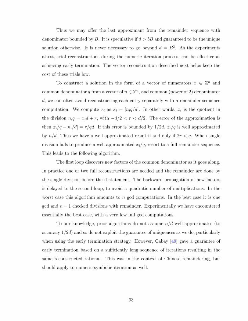
Thus we may offer the last approximant from the remainder sequence with

denominator bounded by B. It is speculative if d > bB and guaranteed to be the unique

solution otherwise. It is never necessary to go beyond d = B2. As the experiments

attest, trial reconstructions during the numeric iteration process, can be effective at

achieving early termination. The vector reconstruction described next helps keep the

cost of these trials low.

To construct a solution in the form of a vector of numerators x ∈ Zn and

common denominator q from a vector of n ∈ Zn, and common (power of 2) denominator

d, we can often avoid reconstructing each entry separately with a remainder sequence

computation. We compute xi as xi = [niq/d]. In other words, xi is the quotient in

the division niq = xid + r, with −d/2 < r < d/2. The error of the approximation is

then xi/q − ni/d| = r/qd. If this error is bounded by 1/2d, xi/q is well approximated

by n/d. Thus we have a well approximated result if and only if 2r < q. When single

division fails to produce a well approximated xi/q, resort to a full remainder sequence.

This leads to the following algorithm.

The first loop discovers new factors of the common denominator as it goes along.

In practice one or two full reconstructions are needed and the remainder are done by

the single division before the if statement. The backward propagation of new factors

is delayed to the second loop, to avoid a quadratic number of multiplications. In the

worst case this algorithm amounts to n gcd computations. In the best case it is one

gcd and n− 1 checked divisions with remainder. Experimentally we have encountered

essentially the best case, with a very few full gcd computations.

To our knowledge, prior algorithms do not assume n/d well approximates (to

accuracy 1/2d) and so do not exploit the guarantee of uniqueness as we do, particularly

when using the early termination strategy. However, Cabay [49] gave a guarantee of

early termination based on a sufficiently long sequence of iterations resulting in the

same reconstructed rational. This was in the context of Chinese remaindering, but

should apply to numeric-symbolic iteration as well.

93

Algorithm 11 Vector DyadicToRational

Input: N ∈ Zn, D ∈ Z. Output: x ∈ Zn, 0 < d ∈ Z, flag, such that flag is “fail” orN/D well approximates x/d and flag is “speculative” or “guaranteed”.d← 1.for i from 1 to n doxi ← [Niq/d].if xi fails the well approximation test thenxi, di, flag = ScalarDyadicToRational(Ni, D).if flag = “fail”, return “fail”.Compute the factorizations d = aig, di = big, where g = gcd(d, di). The newcommon denominator is d ← aidi, so set xi ← xi × ai. Prior numerators mustbe multiplied by bi. Enqueue bi for that later.

end ifend forB ← 1.for i from n down to 1 doxi ← xi ×B;if bi 6= 1 thenB ← B × bi.

end ifend forreturn x, d, flag. [ If any scalar reconstruction was speculative, flag = “speculative”,otherwise flag = “guaranteed”.]

94

4.5 Experiments

For test matrices, we use the following 8 matrix familiesHn, Jn, Qn, Sn,mn,Mn, Rn, Zn

described next.

Hn: The inverse of the n× n Hilbert matrix. This is a famously ill-conditioned

matrix. The condition number of Hn

κ(Hn) = ‖Hn‖2∥∥H−1n ∥∥2 ≈ c 33.97n/

√n

where c is a constant, is quoted in[50]. We find that our numeric solvers – both the

residual norm based and the overlap confirmed continuation approach – can handle

this matrix only up to n = 11. On the other hand, Dixon’s p-adic iteration can handle

any size, provided p is chosen large enough to insure the nonsingularity of Hn mod p.

For instance, Dixon does the n = 100 case in 12 seconds. This class is introduced only

to illustrate the potential for numeric solver failure due to ill-condition.

Jn: This matrix is twice the n × n Jordan block for the eigenvalue 1/2. We

multiply by 2 to get an integer matrix. It is a square matrix with 1’s on the diagonal,

and 2’s on the first subdiagonal. Numerical computations for matrices with repeated

eigenvalues are notoriously difficult. The inverse matrix contains (−2)j on the j-th

subdiagonal. For n > 1023, the matrix J−1n is not representable in double precision

(infinity entries), and for smaller n it poses numerical challenges.

Table 4.1 shows that the numeric-symbolic solvers are faster than the p-adic

lifting when they work, but they have difficulties with Jn.

For n larger than 1023, infinities (numbers not representable in double preci-

sion) defeat all numeric solving. The bottom left entry of J−1n is 2n−1 which is not

representable when n ≥ 1024. However, the overlap solver fails at n = 1023. Although

the inverse matrix itself is just barely representable, some numbers which occur in the

matrix-vector products are not representable in this case.

Qn: Let Qn = DLD, where L is the n×n Lehmer matrix [51, 52], with elements

Li,j = min(i, j)/max(i, j), and D is the diagonal matrix with Di,i = i. Thus Q is an

95

Table 4.1: Dixon is p-adic iteration, Wan is numeric-symbolic iteration using residualnorm based continuation, Overlap is the confirmed continuation methodwe present here.. Times are in seconds.

Examples of numeric failure to convergematrix Dixon Wan OverlapJ994 2.27 1.77 0.0850J995 2.23 fail 0.0920J1022 2.40 fail 0.100J1023 2.38 fail failJ2000 13.3 fail failQ500 2.07 fail 0.81Q1000 15.0 fail 7.29Q2000 121 fail 70.3Q4000 1460 fail 633

integral Brownian matrix [53] with Qi,j = min(i, j)2 (“Q” is for quadratic). A closed

form expression, det(Qn) = 2−n(2n)!/n! follows from [54].

Note that Lx = b iff x = Dy and Qy = Db (also De1 = e1). Being an integer

matrix, Q fits in our experimental framework while rational L does not.

Table 4.1 includes Qn measurements concerning numeric difficulties. In his

recent experiments, Steffy [42] used the Lehmer matrix as an example where Dixon’s

method works but numeric-symbolic iteration does not. We include it here because

it shows a striking difference between residual norm based continuation and overlap

confirmed continuation in numeric-symbolic iteration. In fact, Wan’s code in LinBox

fails on Qn for n > 26.

The examples of Qn along with the remaining five classes of examples are used

for our performance study shown in Table 4.2. These test cases are in many collections

of matrices used for testing. A notable such collection was used by Steffy [42].

Three of our test matrices (Qn,mn, and Mn) are Brownian matrices [53] in that

they have have an “echelon” structure: that is, the elements obey bi,j+1 = bi,j, j > i,

and bi+1,j = bi,j, i > j, for all i, j. Many Brownian matrices have known closed form

96

results for inverses, determinants, factorization, etc. One source of special results is the

following observation [53]. If the matrix P is taken to be a Jordan block corresponding

to a repeated eigenvalue of −1, then PBP T is tridiagonal if and only if B is Brownian.

Sn: The n × n Hadamard matrix using Sylvester’s definition. S1 = (1), S2n = Sn Sn

Sn −Sn

. This definition results in n being a power of two. The determinant

of Sn equals nn/2, which is sharp for the Hadamard bound. Thus, for any integral

right hand side, the solution is a dyadic rational vector. This provides a test of early

termination due to a zero residual.

mn: The n×n matrix with mi,j = min(i, j). Because this a Brownian matrix[53],

PBP T is tridiagonal, and in this case, the tridiagonal matrix is the identity matrix.

Thus, determinant of mn is 1, so the solution is integral for any integral right hand

side. This is another case where early termination due to zero residual is expected.

But the entries in the inverse are larger than in the Hadamard matrix case, so more

iterations may be needed for this example.

Mn: The n × n matrix with Mi,j = max(i, j). The determinant of this matrix

is (−1)n+1n, so the solution vector has denominator much smaller than the Hadamard

bound predicts. The determinant of Mn is found by reversing its rows and columns,

which does not change its determinant. The result is a Brownian matrix. Its tridiagonal

form using the matrix P is the identity matrix — except for the value (−1)nn in the

upper left corner.

The previous three test cases can benefit from early termination. Qn and the

following 2 are expected to benefit less from output sensitivity.

Rn: An n× n matrix with random entries in (−100, 100).

Zn: An n×n {0, 1}-matrix with probability 1/2 of a 1 in a given position. This

is meant to represent some commonly occurring applications. The LinBox library

is often used to compute Smith forms of incidence matrices, where invariant factor

computation involves solving linear systems with random right hand sides.

Reported are run times on a 3.0 GHz Intel Pentium D processor in a Linux

97

2.6.32 environment. All codes used are in LinBox as of svn revision 3639, and have

since been included in the official LinBox release. The experiments were run with

right hand sides being e1, the first column of the identity matrix. This provides a

direct comparison to Steffy’s examples [42] and in some cases allows checking a known

solution formula. But for Qn,Mn, and Zn, the right hand sides used are random with

entries in (−100, 100). This is to create an interesting early termination situation in

the case of Qn and Mn (where the solution for rhs e1 is obtained in the first iteration).

For Zn it is in view of the expected application.

S2k and mn are examples where the determinant is a power of two and con-

siderably less than the Hadamard bound. Thus an early termination due to a perfect

dyadic expansion with residual zero can occur and no rational reconstruction is needed.

Both forms of the Overlap algorithm verify this. The current implementation of Wan’s

method does not check for an exactly zero residual, though there no reason it could

not. The determinant (thus the denominator of solution vector) of Sn is n = 2k and

the Hadamard bound is considerably larger, nn/2. Output sensitive termination due

to zero residual accounts for the factor of 10 or more speedups. The determinant of

mn is 1 and the Hadamard bound is larger than that of Sn. For right hand side e1 the

solution vector is 2e2 − e1 so that essentially no iteration is required if early termina-

tion (Dixon) or zero residual detection (Overlap) is used. In these cases all the time

is in matrix factorization which is about 4 times more costly modulo a prime (Dixon)

than numerically using LAPACK (Overlap). Wan’s implementation lacks the early

termination, thus performs a full iteration. That more than offsets the faster matrix

factorization than in Dixon, making Wan’s implementation slowest for solving with the

mn family.

Mn and Qn results show early termination saving a factor of about 2, the most

available with sufficient dyadic approximation for a guaranteed rational reconstruction.

Further speedup is possible from very early speculative reconstructions. We have not

explored this.

In the data for the random entry matrix, Rn, and random {0, 1}-matrix, Zn, we

98

see variable speedups up to a factor of 1.8 over Dixon’s p-adic lifting, sometimes slightly

aided by early termination. Significant early termination is not generally expected for

these matrix families.

The overlap method works well with sparse numeric solvers (both direct and

iterative), those designed to solve systems where A is sparse. We have begun incor-

porating popular sparse numeric system solvers from packages such as SuperLU [55]

and MATLAB. With these solvers, performance asymptotically better than Dixon’s

method can be expected. Figure 4.1 charts running time of an example computation

comparing the competing dense and sparse exact solvers. The systems used in this

example range from very sparse to barely sparse, increasing density along the x-axis

of the chart. One may notice the crossover points between dotted and solid lines in-

dicating the threshold for switching away from sparse specializations. The significant

symbolic competition to sparse numeric-symbolic will be the method of Eberly, et al.

[56].

99

Figure 4.1: Dense and sparse system performance comparison between the Overlapmethod and Dixon’s method. The measurements are of time taken tosolve systems order 2000, with randomly generated entries in {-100,100}filling each row at the densities listed on the x-axis. There are twopairs of measurements, Dixon’s method (upper pair) and Overlap method(lower). The dotted lines in each case denote runtime of the standarddense approach, while the solid lines measure a specialization for sparsematrices. In the case of the numeric-symbolic solver, this specializationis specifically the use of SuperLU as the numeric solver.

100

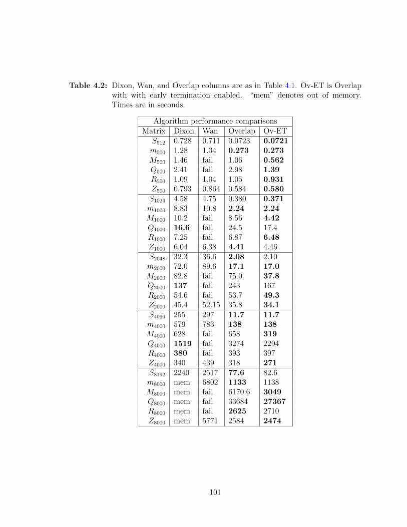
Table 4.2: Dixon, Wan, and Overlap columns are as in Table 4.1. Ov-ET is Overlapwith with early termination enabled. “mem” denotes out of memory.Times are in seconds.

Algorithm performance comparisonsMatrix Dixon Wan Overlap Ov-ETS512 0.728 0.711 0.0723 0.0721m500 1.28 1.34 0.273 0.273M500 1.46 fail 1.06 0.562Q500 2.41 fail 2.98 1.39R500 1.09 1.04 1.05 0.931Z500 0.793 0.864 0.584 0.580S1024 4.58 4.75 0.380 0.371m1000 8.83 10.8 2.24 2.24M1000 10.2 fail 8.56 4.42Q1000 16.6 fail 24.5 17.4R1000 7.25 fail 6.87 6.48Z1000 6.04 6.38 4.41 4.46S2048 32.3 36.6 2.08 2.10m2000 72.0 89.6 17.1 17.0M2000 82.8 fail 75.0 37.8Q2000 137 fail 243 167R2000 54.6 fail 53.7 49.3Z2000 45.4 52.15 35.8 34.1S4096 255 297 11.7 11.7m4000 579 783 138 138M4000 628 fail 658 319Q4000 1519 fail 3274 2294R4000 380 fail 393 397Z4000 340 439 318 271S8192 2240 2517 77.6 82.6m8000 mem 6802 1133 1138M8000 mem fail 6170.6 3049Q8000 mem fail 33684 27367R8000 mem fail 2625 2710Z8000 mem 5771 2584 2474

101

4.6 Summary

In this chapter we detailed a history of leading approaches to the problem of solv-

ing a rational linear system exactly. Specifically we compared and contrasted Dixon’s

p-adic lifting algorithm with Wan’s numeric-symbolic iteration. The two schemes are

asymptotically equivalent, with the numeric-symbolic approach likely to be faster on

most problems due to the advantages of floating point arithmetic versus intermediate

exact computations. However, the (only well-known) implementation of Wan’s idea

in LinBox was hardly reliable for a wide class of input problems. We addressed this

shortcoming, simultaneously improving runtime performance, with our overlap method

to provide confirmed-continuation of the algorithm. The key reason this improvement

was successful is that it is adaptive to the level of accuracy provided by the numeric

solver, and is much less pessimistic regarding intermediate results. Additionally, the

improved rational reconstruction component allows for output-sensitive, speculative or

guaranteed early termination, which has also been shown beneficial to certain exam-

ples. Having a robust rational system solver is not only an important routine to be used

directly, but also an important kernel used by many solutions that LinBox provides,

for example computing null space basis, the last invariant factor, or the Smith normal

form. Many applications stand to benefit from our improvement to the performance

and stability of the numeric-symbolic solver.

102

Chapter 5

SUMMARY

In this thesis we have used LinBox as a vehicle for developing solutions to

select exact linear algebra problems. These solutions have in some cases improved on

the performance of preexisting approaches, and in other cases enabled computation of

previously unexplored problems. As computing hardware is advancing, so too must

exact computational linear algebra’s algorithms and computational methods.

In Chapter 2 we have markedly improved arithmetic over small prime finite

fields in LinBox. Performing faster arithmetic over these fields lends performance to

the many algorithms in exact linear algebra of which field arithmetic is a building

block.. These improvements have not only improved wall-clock performance on the

bare hardware, but also lowered the memory requirements for storing the finite field

data. Both benefits stand to help future LinBox developers push the boundaries on the

scope of computable problems. First, we outlined the more widely-known compression,

bit-packing, which is quite flexible and even extendible. Our primary extension, that

of semi-normalization has proven significantly more efficient for certain small-prime

fields. Next, we detailed the lesser-known strategy of bit-slicing for F3 in LinBox and

demonstrated that it is without a doubt the state of the art in representing matrices

consisting of this particular field’s elements. We provide an implementation of these

compression methods in LinBox. We have demonstrated the efficacy of these compres-

sion schemes with repeatable experiments containing dependably regular performance

improvements.

An immediate application of these advancements in finite field arithmetic ap-

peared in Chapter 3. Here we calculated the 3-rank of a 316×316 matrix, which involved

computing with over 1.85 peta-entries. This project relied every bit on the efficient

103

compression schemes, but also required the development of a novel Monte Carlo algo-

rithm when preexisting solutions proved to run too long or ballooned memory usage

too large. Additionally, various flavors of parallelism were needed to solve this problem,

especially considering the number of times the computation needed to be restarted due

to bugs, oversights, heuristic adjustments, and the like. These failures that happened

along the way taught valuable lessons about distributed computing algorithm design,

especially when storing large amounts of data is an algorithmic requirement.

Specifically three types of parallelism were triumphantly melded together in or-

der to solve this large problem. First, the word-level parallelism of bit-slicing ensured

that each CPU cycle devoted to finite-field arithmetic was computing on sixty-four

values at a time. Second, as the subject matrix of our rank calculation was not stored

a priori but generated on-demand by a position-independent formula, shared-memory

parallelism was employed. This was an ideal solution to quickly generating the needed

matrix entries, especially considering our access to a super computer with highly effi-

cient, 48-core nodes. Finally, speaking in terms of managing both long running time

and large memory demands, a distributed decomposition or “chunking” of the problem

into units of work manageable by these compute nodes was an absolute necessity. The

goal was to spread computation, and by extension storage responsibility, to as many

compute nodes as possible. To accomplish this delegation of tasks, an RPC-based,

master-slave, work-queueing framework was developed and successfully employed.

In Chapter 4 I describe and evaluate the new, state of the art, numeric-symbolic

rational linear system solver that we created. For many cases of wanting an exact

solution to a linear system, our solver performs better than the previously leading

exact algorithm, Dixon’s method. In all cases, the new solver outperforms and is

less sensitive to troublesome input problems than its immediate predecessor, Wan’s

numeric-symbolic method. The difference of the new method is what we call confirmed-

continuation, which is a method of detecting optimistic overlap between iterations of

the solver. In any case, the modularization of the highly-tuned numeric linear algebra

kernel we choose to use ensures we can always integrate with the bleeding-edge of

104

scientific research in floating-point linear algebra. Many of these kernels have been

specialized for specifically structured input, providing a great degree of flexibility in

efficiently solving different systems exactly. Solving rational linear systems is a key

solution offered by LinBox to its users.

5.1 Future Work

With the foundations in place that have been vetted to solve known large prob-

lems, the final goal for bit-packing and bit-slicing implementations is to provide a clean,

usable interface so that many LinBox kernels and developers can take advantage of

these new data representations. Hand-vectorizing the arithmetic loops employed by

these compression schemes will certainly pay off, especially as chip manufacturers con-

tinue to push wider and wider registers and vectorization instruction sets. Regarding

the large 3-rank problem, the new theoretical algorithm and implemented parallel

framework are general enough to apply to graph families similar to Dickson, where

the sequence of ranks is also sought. Each of these cases may require tweaking of the

heuristic approach used to compress the rank of the large matrix into a manageable

block size. Ever-larger computations will follow, in lock-step with the improvements

to hardware and abundance of memory and disk storage space. Having arrived at the

rank of D(3, 8) in a few days, the asymptotic complexity suggests we can expect on-

going computations to take on the order of months to complete. It is truly exciting to

push ever forward with this framework.

105

BIBLIOGRAPHY

[1] J-G. Dumas, T. Gautier, M. Giesbrecht, P. Giorgi, B. Hovinen, E. Kaltofen, B. D.Saunders, W. Turner, and G. Villard. Linbox: A generic library for exact linearalgebra. In ICMS’02, pages 40–50, 2002.

[2] M. Flynn. Some computer organizations and their effectiveness. Computers, IEEETransactions on, C-21(9):948–960, Sept 1972.

[3] Brian W. Kernighan and Dennis M. Ritchie. The C Programming Language.Prentice Hall Professional Technical Reference, 2nd edition, 1988.

[4] P.J. Plauger, Meng Lee, David Musser, and Alexander A. Stepanov. C++ Stan-dard Template Library. Prentice Hall PTR, Upper Saddle River, NJ, USA, 1stedition, 2000.

[5] T. J. Boothby and R. W. Bradshaw. Bitslicing and the Method of Four RussiansOver Larger Finite Fields. ArXiv e-prints, January 2009.

[6] Martin Albrecht, Gregory Bard, and William Hart. Efficient multiplication ofdense matrices over gf(2). CoRR, abs/0811.1714, 2008.

[7] Martin Albrecht and Gregory Bard. The M4RI Library – Version 20100817. TheM4RI Team, 2010.

[8] Jeffrey Sheldon, Walter Lee, Ben Greenwald, and Saman Amarasinghe. Strengthreduction of integer division and modulo operations. In HenryG. Dietz, editor,Languages and Compilers for Parallel Computing, volume 2624 of Lecture Notesin Computer Science, pages 254–273. Springer Berlin Heidelberg, 2003.

[9] B. David Saunders and Bryan S. Youse. Large matrix, small rank. In Proceedingsof the 2009 international symposium on Symbolic and algebraic computation, InProc. of ISSAC 2009, pages 317–324, New York, NY, USA, 2009. ACM.

[10] J G Dumas and G Villard. Computing the rank of large sparse matrices overfinite fields. In CASC’2002 Computer Algebra in Scientific Computing, pages 22–27. Springer-Verlag, 2002.

[11] B. A. LaMacchia and A.M. Odlyzko. Solving large sparse linear systems over finitefields. Lecture Notes in Computer Science, 537:109–133, 1991.

106

[12] J-G. Dumas, B. D. Saunders, and G. Villard. Smith form via the valence: Expe-rience with matrices from homology. In Proc. of ISSAC’00, pages 95–105. ACMPress, 2000.

[13] J.-C. Faugere. Parallelization of Grobner basis. In H. Hong, editor, PASCO’94,volume 5 of Lecture notes series in computing, pages 109–133, 1994.

[14] Guobiao Weng, Weisheng Qiu, Zeying Wang, and Qing Xiang. Pseudo-paleygraphs and skew hadamard difference sets from presemifields. Designs, Codes andCryptography, 44(1-3):49–62, 2007.

[15] J.P May, B.D. Saunders, and Z. Wan. Efficient matrix rank computation withapplication to the study of strongly regular graphs. In In Proc. of ISSAC 2007,pages 277–284. ACM Press, 2007.

[16] Q. Xiang. Recent progress in algebraic design theory. Finite Fields and TheirApplications, 11:622–653, 2005.

[17] T. Cormen, C. Leiserson, R. Rivest, and C. Stein. Introduction to Algorithms,Second edition. MIT Press, 2001.

[18] D. Wiedemann. Solving sparse linear equations over finite fields. IEEE Trans.Inform. Theory, 32:54–62, 1986.

[19] E. Kaltofen and B. D. Saunders. On Wiedemann’s method of solving sparse linearsystems. In Applied Algebra, Algebraic Algorithms and Error-Correcting Codes,volume 539 of LNCS, pages 29–38, 1991.

[20] E. Kaltofen. On probabilistic analysis of randomization in hybrid symbolic-numeric algorithms, http://www4.ncsu.edu/~kaltofen/bibliography/07/

K07_owr_abs.pdf. In Oberwolfach Reports, volume 4, 2007.

[21] G. Cooperman and G. Havas. Elementary algebra revisited: Randomized algo-rithms. In P. Pardalos, S. Rajasekaran, and J. Rolim, editors, Proc. of DIMACSWorkshop on Randomization Methods in Algorithm Design, number 43 in DI-MACS Series in Discrete Mathematics and Theoretical Computer Science, pages37–44. AMS, Providence, RI, 1998.

[22] L. Chen, W. Eberly, E. Kaltofen, W. Turner, B. D. Saunders, and G. Villard.Efficient matrix preconditioners for black box linear algebra. LAA 343-344, 2002,pages 119–146, 2002.

[23] W. Turner. Preconditioners for singular black box matrices. In Proc. of ISSAC’05,pages 332–339, New York, NY, USA, 2005. ACM Press.

[24] E. Kaltofen and B. D. Saunders. On Wiedemann’s method of solving sparse linearsystems. In Proc. AAECC-9, volume 539 of Lect. Notes Comput. Sci., pages 29–38.Springer Verlag, 1991.

107

[25] J.T. Schwartz. Fast probabilistic algorithms for verification of polynomial identi-ties. J. ACM, pages 27:701–717, 1980.

[26] R. Zippel. Interpolating polynomials from their values. J. Symb. Comp., 9(3):375–403, 1990.

[27] S. L. Ma. A survey of partial difference sets. Designs, Codes and Cryptography,4:221–261, 1994.

[28] Thierry Gautier, Jean-Louis Roch, and Gilles Villard. Givaro, a C++ for algebraiccomputations. http://givaro.forge.imag.fr.

[29] Edsger W. Dijkstra. The origin of concurrent programming. chapter Cooperatingsequential processes, pages 65–138. Springer-Verlag New York, Inc., New York,NY, USA, 2002.

[30] William Gropp, Ewing Lusk, and Anthony Skjellum. Using MPI (2Nd Ed.):Portable Parallel Programming with the Message-passing Interface. MIT Press,Cambridge, MA, USA, 1999.

[31] Bryan Youse. Finite field/rank code suite. https://bitbucket.org/bryouse/

finite-field-rank-suite.

[32] OpenMP Architecture Review Board. OpenMP application program interfaceversion 3.0, May 2008.

[33] Donald E. Knuth. The Art of Computer Programming, Volume 2 (3rd Ed.):Seminumerical Algorithms. Addison-Wesley Longman Publishing Co., Inc.,Boston, MA, USA, 1997.

[34] Zhengdong Wan. An algorithm to solve integer linear systems exactly using nu-merical methods. Journal of Symbolic Computation, 41:621–632, 2006.

[35] Zhengdong Wan. Computing the Smith Forms of Integer Matrices and SolvingRelated Problems. PhD thesis, University of Delaware, Newark, DE, 2005.

[36] Keith O. Geddes and Wei Wei Zheng. Exploiting fast hardware floating point inhigh precision computation. In J. Rafael Sendra, editor, ISSAC, pages 111–118.ACM, 2003.

[37] Alicja Smoktunowicz and Jolanta Sokolnicka. Binary cascades iterative refinementin doubled-mantissa arithmetics. BIT, 24(1):123–127, 1984.

[38] Andrzej Kie lbasinski. Iterative refinement for linear systems in variable-precisionarithmetic. BIT, 21(1):97–103, 1981.

[39] J. D. Dixon. Exact solution of linear equations using p-adic expansion. Numer.Math., pages 137–141, 1982.

108

[40] Nicholas J. Higham. Accuracy and Stability of Numerical Algorithms. Society forIndustrial and Applied Mathematics, Philadelphia, PA, USA, 2nd edition, 2002.

[41] James H. Wilkinson. Rounding Errors in Algebraic Processes. Dover Publications,Incorporated, 1994.

[42] Daniel Steffy. Exact solutions to linear systems of equations using output sensitivelifting. ACM Communications in Computer Algebra, 44(4):160–182, 2010.

[43] The LinBox Team. LinBox, a C++ library for exact linear algebra. http://www.linalg.org/.

[44] Z. Chen and A. Storjohann. A BLAS based C library for exact linear algebra oninteger matrices. In Proc. of ISSAC’05, pages 92–99. ACM Press, 2005.

[45] T. Mulders and A. Storjohann. Certified dense linear system solving. Jounal ofsymbolic computation, 37(4), 2004.

[46] Torbjorn Granlund and the GMP development team. GNU MP: The GNU Mul-tiple Precision Arithmetic Library, 5.0.5 edition, 2012. http://gmplib.org/.

[47] Mark van Hoeij and Michael B. Monagan. A modular gcd algorithm over numberfields presented with multiple extensions. In Teo Mora, editor, ISSAC, pages109–116. ACM, 2002.

[48] Joachim Von Zur Gathen and Jurgen Gerhard. Modern Computer Algebra. Cam-bridge University Press, New York, NY, USA, 2 edition, 2003.

[49] Stanley Cabay. Exact solution of linear equations. In Proceedings of the secondACM symposium on Symbolic and algebraic manipulation, SYMSAC ’71, pages392–398, New York, NY, USA, 1971. ACM.

[50] Bernhard Beckermann. The condition number of real Vandermonde, Krylov andpositive definite Hankel matrices. Numerische Mathematik, 85:553–577, 1997.

[51] John Todd. Basic Numerical Mathematics, Vol. 2: Numerical Algebra. Birkhauser,Basel, and Academic Press, New York, 1977.

[52] D. H. Lehmer. Solutions to problem E710, proposed by D. H. Lehmer: The inverseof a matrix, November 1946.

[53] M. J. C. Gover and S. Barnett. Brownian matrices: properties and extensions.International Journal of Systems Science, 17(2):381–386, 1986.

[54] E. Kilic and P. Stanica. The Lehmer matrix and its recursive analogue. Journal ofCombinatorial Mathematics and Combinatorial Computing, 74(2):195–205, 2010.

[55] SuperLU User’s Guide: http: // www. nersc. gov/ ~ xiaoye/ SuperLU/ , 2003.

109

[56] W. Eberly, M. Giesbrecht, P. Giorgi, A. Storjohann, and G. Villard. Solving sparserational linear systems. In Proc. of ISSAC’06, pages 63–70. ACM Press, 2006.

110

Appendix A

REMOTE OBJECTS WITH PYRO

Setting up objects for remote procedure calls is made easy by the PyRO (Python

Remote Objects) package. The scenario is that the master Python script from Sec-

tion 3.3.3.1 wants to share the BlockManager object across the network to machines

that will serve as workers (be they producers or consumers). The code to set this up

is a simple snippet:

import Pyro4

... define BlockManager ...

# make a Pyro daemondaemon=Pyro4.Daemon(host="chimera.cis.udel.edu")# find the name servernameserver=Pyro4.locateNS("chimera.cis.udel.edu")

manager=BlockManager() # the central, shared manager

uri=daemon.register(manager) # register as a PyRO objectns.register("manager", uri) # register in the name server

daemon.requestLoop() # event loop server; wait for remote calls

There are two components at play here. First, creating a daemon and registering

the BlockManager object with this daemon. The daemon is then started; here PyRO

loops indefinitely, waiting for remote hosts to connect. Second, registering the object

with a PyRO name server. The name server is a separate process, started indepen-

dently, that maps the long URI PyRO allocates for our object to an easy-to-remember

name. This is the same concept behind the broadly used DNS system on the Internet,

which relates numeric IP addresses into memorable hostnames. Thus, instead of a long

111

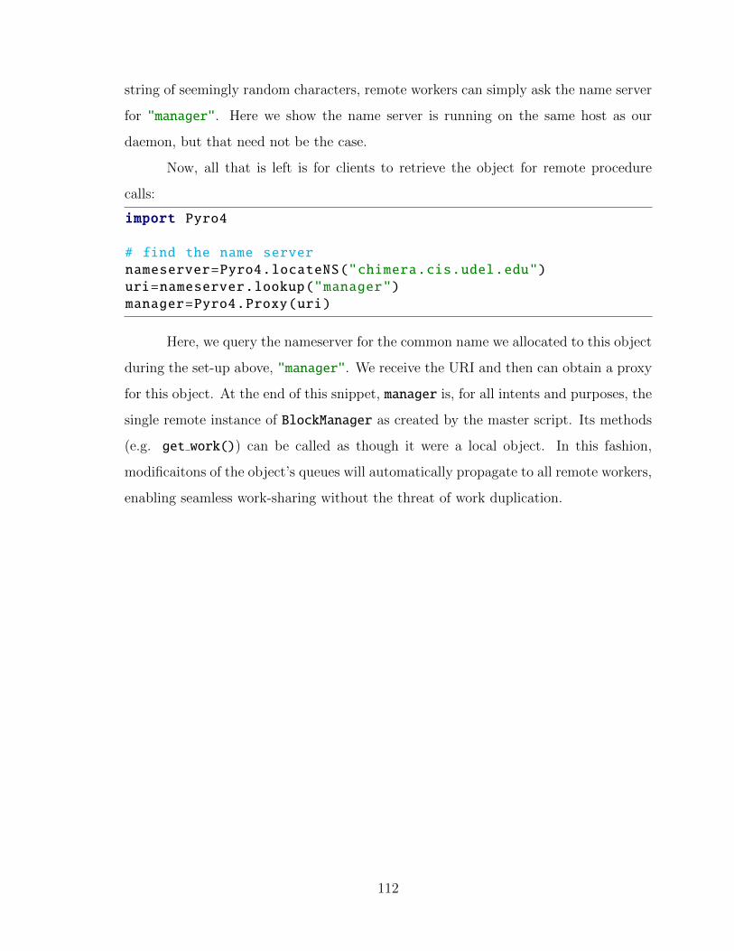
string of seemingly random characters, remote workers can simply ask the name server

for "manager". Here we show the name server is running on the same host as our

daemon, but that need not be the case.

Now, all that is left is for clients to retrieve the object for remote procedure

calls:

import Pyro4

# find the name servernameserver=Pyro4.locateNS("chimera.cis.udel.edu")uri=nameserver.lookup("manager")manager=Pyro4.Proxy(uri)

Here, we query the nameserver for the common name we allocated to this object

during the set-up above, "manager". We receive the URI and then can obtain a proxy

for this object. At the end of this snippet, manager is, for all intents and purposes, the

single remote instance of BlockManager as created by the master script. Its methods

(e.g. get work()) can be called as though it were a local object. In this fashion,

modificaitons of the object’s queues will automatically propagate to all remote workers,

enabling seamless work-sharing without the threat of work duplication.

112

Appendix B

F3 BIT-SLICING “STEPPER”

As explained in Section 2.3 and specifically demonstrated by Algorithm 5, bit-

slicing data is an involved process containing pointer arithmetic, bit-shifting and mask-

ing operations.. When initializing a bit-sliced matrix or vector, it would be no quick

and simple task, computationally speaking, to perform calls to LinBox’s setEntry()

for each F3 element to be encoded. This is where the concept of a “Stepper” comes

in. Rather than insert elements entry-by-entry, insertions can be pooled until there are

enough of them to fill up the sliced words. Again, sliced words are the machine words

comprising sliced units, which themselves are the building blocks of bit-slicing. A class

which is intended to be subclassed is used for this purpose:

class Stepper {

public:inline void step(uint8 t e) {

store[ i −−] = e;if( i > width) flush();

}

virtual inline void flush() = 0;

inline void row(){if( i != width −1) flush();

}

private:uint8 t ∗ store;size t i;size t width;

};

The Stepper interface contains three functions:

113

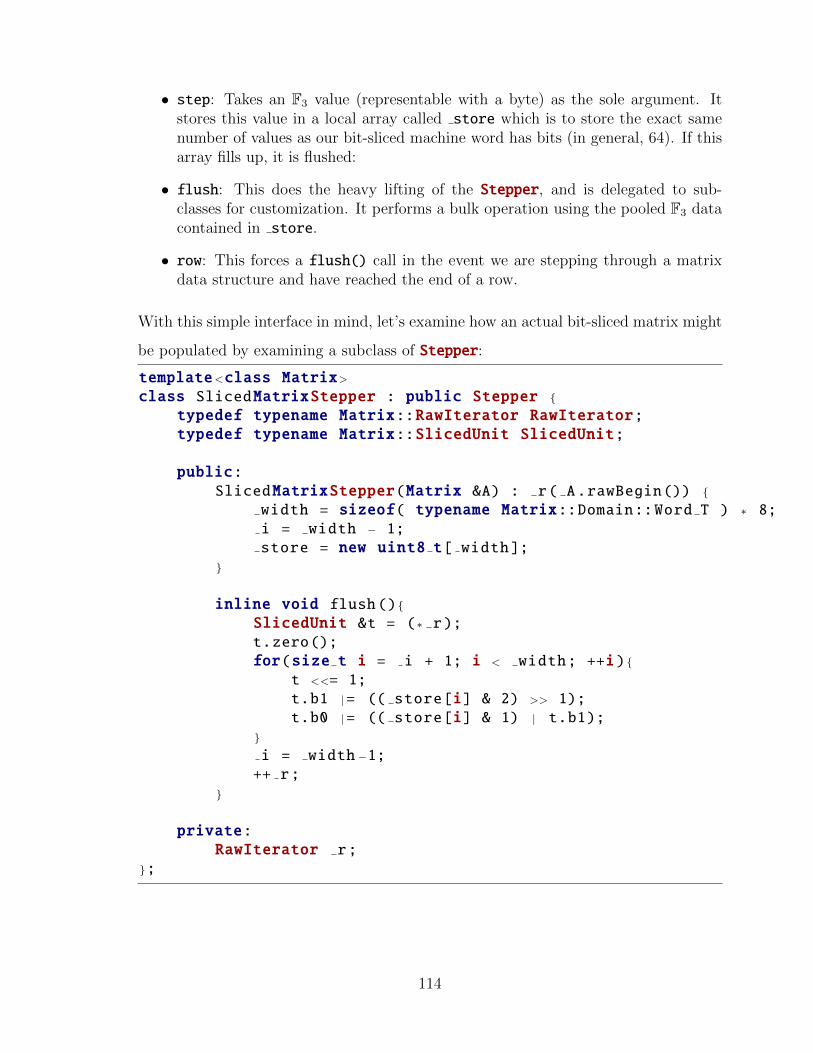
• step: Takes an F3 value (representable with a byte) as the sole argument. Itstores this value in a local array called store which is to store the exact samenumber of values as our bit-sliced machine word has bits (in general, 64). If thisarray fills up, it is flushed:

• flush: This does the heavy lifting of the Stepper, and is delegated to sub-classes for customization. It performs a bulk operation using the pooled F3 datacontained in store.

• row: This forces a flush() call in the event we are stepping through a matrixdata structure and have reached the end of a row.

With this simple interface in mind, let’s examine how an actual bit-sliced matrix might

be populated by examining a subclass of Stepper:

template<class Matrix>class SlicedMatrixStepper : public Stepper {

typedef typename Matrix::RawIterator RawIterator;typedef typename Matrix::SlicedUnit SlicedUnit;

public:SlicedMatrixStepper(Matrix &A) : r( A.rawBegin()) {

width = sizeof( typename Matrix::Domain::Word T ) ∗ 8;i = width − 1;store = new uint8 t[ width];

}

inline void flush (){SlicedUnit &t = ( ∗ r);t.zero();for(size t i = i + 1; i < width; ++i) {

t <<= 1;t.b1 | = (( store[i] & 2) >> 1);t.b0 | = (( store[i] & 1) | t.b1);

}

i = width −1;++ r;

}

private:RawIterator r;

};

114

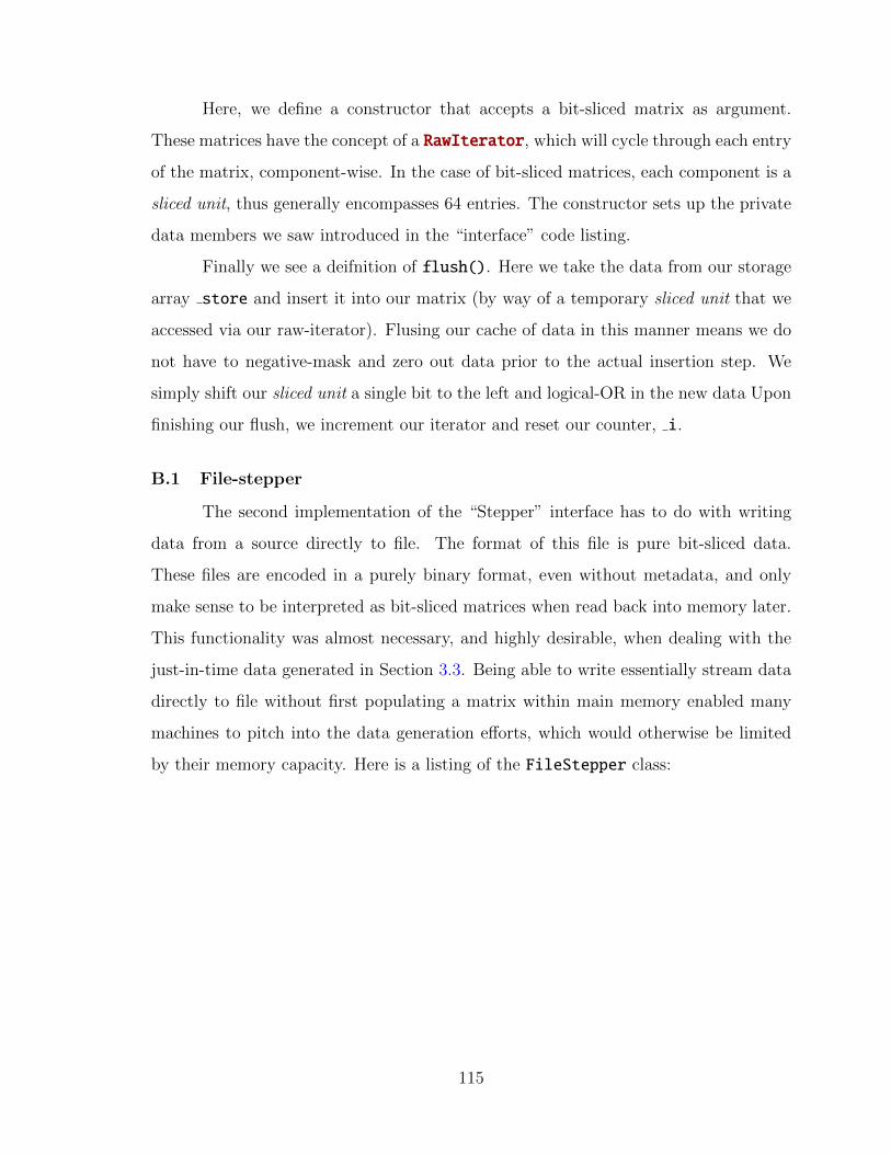
Here, we define a constructor that accepts a bit-sliced matrix as argument.

These matrices have the concept of a RawIterator, which will cycle through each entry

of the matrix, component-wise. In the case of bit-sliced matrices, each component is a

sliced unit, thus generally encompasses 64 entries. The constructor sets up the private

data members we saw introduced in the “interface” code listing.

Finally we see a deifnition of flush(). Here we take the data from our storage

array store and insert it into our matrix (by way of a temporary sliced unit that we

accessed via our raw-iterator). Flusing our cache of data in this manner means we do

not have to negative-mask and zero out data prior to the actual insertion step. We

simply shift our sliced unit a single bit to the left and logical-OR in the new data Upon

finishing our flush, we increment our iterator and reset our counter, i.

B.1 File-stepper

The second implementation of the “Stepper” interface has to do with writing

data from a source directly to file. The format of this file is pure bit-sliced data.

These files are encoded in a purely binary format, even without metadata, and only

make sense to be interpreted as bit-sliced matrices when read back into memory later.

This functionality was almost necessary, and highly desirable, when dealing with the

just-in-time data generated in Section 3.3. Being able to write essentially stream data

directly to file without first populating a matrix within main memory enabled many

machines to pitch into the data generation efforts, which would otherwise be limited

by their memory capacity. Here is a listing of the FileStepper class:

115

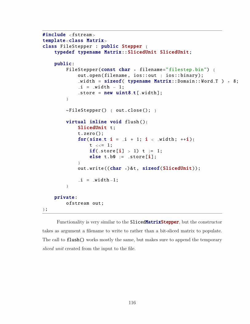
#include <fstream>template<class Matrix>class FileStepper : public Stepper {

typedef typename Matrix::SlicedUnit SlicedUnit;

public:FileStepper(const char ∗ filename="filestep.bin") {

out.open(filename, ios::out | ios::binary);width = sizeof( typename Matrix::Domain::Word T ) ∗ 8;i = width − 1;store = new uint8 t[ width];

}

~FileStepper() { out.close(); }

virtual inline void flush (){SlicedUnit t;t.zero();for(size t i = i + 1; i < width; ++i) {

t <<= 1;if( store[i] > 1) t | = 1;else t.b0 | = store[i];

}

out.write((char ∗)&t, sizeof(SlicedUnit));

i = width −1;}

private:ofstream out;

};

Functionality is very similar to the SlicedMatrixStepper, but the constructor

takes as argument a filename to write to rather than a bit-sliced matrix to populate.

The call to flush() works mostly the same, but makes sure to append the temporary

sliced unit created from the input to the file.

116