High-order Well-balanced Schemes

Sebastian Noelle, Yulong Xing, Chi-Wang Shu

Contents1. Introdu tion (3).2. Preliminaries: steady states and the residual (5).3. S hemes based on well-balan ed nite dieren e operators (8).4. S hemes based on well-balan ed quadrature (23).5. Numeri al examples for the shallow water equations (39).6. Con lusion (60).

3Abstra tIn this paper we review some re ent work on high-order well-balan eds hemes for hyperboli systems of balan e laws. A hara teristi featureof su h systems is the existen e of non-trivial steady state solutions,where the ee ts of onve tive uxes and sour e terms an el ea h other.Well-balan ed s hemes satisfy a dis rete analogue of this balan e andare therefore able to maintain a steady state. We dis uss two lassesof s hemes, one based on high-order a urate, non-os illatory nite dif-feren e operators whi h are well-balan ed for a general lass of steadystates, and the other one based on well-balan ed quadratures, whi h an- in prin iple - be applied to all steady states. Hyperboli systems ofbalan e laws have a wide appli ation, exemplied by shallow water equa-tions (SWE) whi h have steady states at rest, where the ow velo ityvanishes, and also the more hallenging moving ow steady states. Nu-meri al experiments show ex ellent resolution of unperturbed as well asslightly perturbed steady states.Keywords: shallow water equations, fundamental steady states, high-order upwind nite volume s hemes, well-balan ed s hemes1. IntroductionIn many appli ations we en ounter hyperboli balan e laws, whi h in onedimension are in the form(1.1) Ut + f(U, x)x = s(U, x)where U is the solution ve tor, f(U, x) is the ux and s(U, x) is the sour e term.The sour e term may ome from geometri al, rea tive or other onsiderations.Examples of hyperboli balan e laws in lude the shallow water equation with anon-at bottom topology, elasti wave equation [2, hemosensitive movement[16 and nozzle ow [14.Comparing with the standard hyperboli onservation laws, namely (1.1)with s(U, x) = 0, the numeri al approximation to the balan e laws (1.1) isusually not too mu h more di ult: we simply need to put the point values

4(for nite dieren e s hemes) or the ell averages (for nite volume s hemes) ofthe sour e term s(U, x) dire tly into the dis retization of the spatial operator.There is, however, one noti eable ex eption. The balan e law (1.1) often admitssteady state solutions in whi h the sour e term s(U, x) is exa tly balan edby the ux gradient f(U, x)x. Su h steady state solutions are usually non-trivial (they are usually not polynomial fun tions of the spa ial variable x)and they often arry important physi al meaning (for example, the still wateror steady moving water solution of the shallow water equation, to be studiedin more detail later in this paper). The obje tive of well-balan ed s hemes isto preserve exa tly some of these steady state solutions. The most importantadvantage of well-balan ed s hemes is hat they an a urately resolve smallperturbations to su h steady state solutions with relatively oarse meshes. In omparison, a non-well-balan ed s heme will introdu e trun ation errors to thesteady state solution, hen e it annot resolve small perturbations to su h steadystates unless the trun ation error is already smaller than su h perturbations,thus requiring a rened mesh. In Se tion 5 we will provide su h examples.However, it is quite di ult to design well-balan ed s hemes whi h are high-order a urate and non-os illatory in the presen e of dis ontinuities in thesolution.In this paper we use the shallow water equation as a prototype to survey afew re ently developed well-balan ed high-order nite dieren e, nite volumeand dis ontinuous Galerkin nite element methods. We attempt to explainthe main ingredients in these algorithms whi h allow us to a hieve the well-balan ed property without losing other ni e properties of the original s heme,su h as high-order a ura y and non-os illatory performan e in the presen e ofsolution dis ontinuities.The paper is organized as follows. In Se tion 2 we rst dis uss a numberof interesting steady states. Then we introdu e the residual whi h need to bewell-balan ed near stationary states.At this point the paper splits into two approa hes: The rst approa h, seeSe tion 3, applies to nite dieren e, nite volume and dis ontinuous Galerkins hemes. It treats steady states for whi h the sour e term an be de omposedinto sums of produ ts of the form (3.4). The hallenge is to onstru t nite

5dieren e operators whi h are high-order a urate and non-os illatory for the onservative ux dieren e and the sour e term, and whi h oin ide for bothterms in the ase of steady state solutions.The se ond approa h, designed for general steady states and nite volumes hemes, is overed in Se tion 4. The key task is to nd well-balan ed quadra-tures for the integral of the residual, see equation (4.1). Subse tion 4.2 presentsa general framework to de ompose this integral into suitable parts. Subse -tion 4.3 realizes this approa h for moving water steady states for shallow waterows.In Se tion 5 we present numeri al results showing the a ura y and well-balan ed properties of both lasses of s hemes for a number of hallenging ows.Se tion 6 ontains some on luding remarks.It is perhaps surprising that the two approa hes outlined in Se tions 3 and4 require su h dierent te hniques. Indeed, the reader might skip either se tionon a rst reading, and then pro eed to the numeri al experiments in Se tion 5.On the other hand, we hope that the presentation of both approa hes ina single paper will provide a lear understanding that well-balan ing requiresa detailed study of the trun ation error for ea h individual s heme (sin e thetrun ation error should disappear for dis rete steady states). The broad setof ideas and te hniques presented in this paper might be helpful to the readerdeveloping his/her own version of high-order well-balan ing in a new situation.2. Preliminaries: steady states and the residualIn this se tion we introdu e equilibrium variableswhi h hara terize smoothsteady states, and dis uss the residual whi h monitors the deviation of thesystem from stationary states. In parti ular, two forms of the residual aresingled out whi h are the bases of the nite dieren e algorithms in Se tion 3on one hand and the nite volume algorithm in Se tion 4 on the other hand.We will generally refer to a time-independent solution of the hyperboli balan e law as a steady state. When we refer to pointwise or ell-wise lo altransformations, we may use the terms equilibrium-transvormation, -variable,-re onstru tion, -limiting and so forth.

62.1. Steady statesLet us again onsider the system of balan e laws (1.1). For example, forthe shallow water equationsU = (h, m)T , f(U) = (m, m2/h + gh2/2)T , s(U, x) = (0,−ghbx(x))T ,(2.1)where h is the water height, m is the momentum (dis harge in hydrauli s), b(x)is the pres ribed bottom topography above a given referen e height, and g isthe gravitational a eleration.Many su h systems an be rewritten in the form

Vt + c(V, x)Vx = 0(2.2)for some variableV = V (U, x),(2.3)whi h we would like to all the equilibrium variables, sin e onstant V impliesa stationary state.Note that onstant V does not imply that U is onstant, sin e V dependsalso on x through the variable fun tion b. Therefore, one should expe t non-trivial steady states.For shallow water, the equilibrium variables are V (U, x) = (m, E), wherethe equilibrium energy E is given by

E(U, b) =m2

2h2+ g(h + b).(2.4)In the following we des ribe various lasses E of stationary states.Example 2.1 - (1) The lass of all steady states, Etot.(2) Smooth steady states Esmooth.(3) Conservation laws: Here s(U, b) ≡ 0 and f(U) ≡ const. Stationary statesin lude

• E0 = onstant states.• E1 = two onstant states separated by a stationary sho k or onta t.

7• E2 = gas dynami s with zero velo ity, onstant pressure, and any boundedmeasurable fun tion for the density.(4) Steady states for 1D s alar balan e laws.(5) 1D shallow water equations:• The lake at rest ELaR, where m ≡ 0 and hen e E = g(h + b) ≡ const.• Smooth river ows Eriver, where m is nonzero.• Waterfalls Ewaterfall (dis ontinuous river ows)(6) Separable sour e terms studied in [36.(7) Geostrophi jets Ejet for 2D shallow water, where (u, v) ≡ (u(y), 0), g(h +

b)y = fu and f is the oriolis for e in the upper hemisphere.(8) Multi-layer shallow water: O eans at rest and moving o eans.Remark 2.1 - (1) There are many more lasses of steady states, espe ially in2D.(2) It is important to note that most well-balan ed s hemes are designed topreserve only a ertain sub lass of steady states exa tly. Other steady statesmay be preserved approximately within a ertain order of a ura y.Se tion 3 treats steady states for whi h the sour e terms are separable inthe sense of (3.4). This in ludes the lake at rest as a prototype. The maintool is the onstru tion of a well-balan ed lass of nite dieren e operators.In Se tion 4 we outline a well-balan ed nite volume approa h. While theframework in Subse tion 4.1 overs in prin iple all steady states, we arry outthe spe i steps for moving water ows in Subse tion 4.3.2.2. The residualLet us again onsider the system of balan e laws (1.1). We are parti ularlyinterested in solutions lose to steady states, where Ut = 0. Therefore, weintrodu e the residualR := −f(U)x + s(U, x).(2.5)

8Note thatUt = R,(2.6)and the solution U deviates from steady state if and only if R 6= 0.In Se tion 3 we will study a lass of separable steady states satisfying (3.4).This assumption implies that

R = (−f(U) + t(U, x))x(2.7)for stationary solutions, where t(U, x) is determined by s(U, x). Using thisstru ture, we onstru t high-order a urate well-balan ed nite dieren e op-erators.In Se tion 4 we fo us on nite volume s hemes and hen e onsider ellaverages Ri of the residual. Well-balan ed quadratures are onstru ted for theregular and singular parts of these integrals.3. Schemes based on well-balanced finite difference operatorsIn this se tion, we fo us on a lass of steady states for whi h the sour eterm is separable in the sense of Assumption 3.2. We develop well-balan edhigh-order a urate nite dieren e operators for the residual. Based on thesedieren e operators, we derive well-balan ed nite dieren e, nite volume anddis ontinuous Galerkin s hemes. The steady states under onsideration in ludethe lake at rest for the shallow water equations.The one-dimensional hyperboli system of onservation laws with sour eterms under onsideration is given by (1.1). We start the dis ussion by present-ing the well balan ed nite dieren e s heme. The extension to nite volumeand DG s hemes is shown in the following subse tions. Only one-dimensionalbalan e law (1.1) is investigated in this se tion, although the generalization tothe multi-dimensional ase(3.1) Ut + f(U, x, y)x + g(U, x, y)y = s(U, x, y) an be done in some situations. For example, we an easily generalize theproposed te hnique to the two-dimensional shallow water equations with lakeat rest steady state.

93.1. Finite dieren e s hemeWe rst onsider the ase that (1.1) is a s alar balan e law. The ase ofsystems will be explored later. We are interested in preserving exa tly ertainsteady state solutions U of (1.1):(3.2) f(U)x = s(U, x).We make two assumptions on the equation (1.1) and the steady state solutionU of (3.2) that we are interested to preserve exa tly.Assumption 3.1. The steady state solution U of (3.2) that we are interestedto preserve satises(3.3) V (U, x) = constantfor a known fun tion V (U, x).Note that in [34, 35, 36 the equilibrium variables have been denoted bya(U, x) instead of V (U, x).Assumption 3.2. The sour e term s(U, x) in (1.1) an be de omposed as(3.4) s(U, x) =

∑

i

si(V (U, x)) t′i(x)for some fun tions si and ti.We will design a numeri al s heme whi h an preserve exa tly the steadystate solutions U whi h satisfy Assumption 3.1, for a balan e law (1.1) witha sour e term satisfying Assumption 3.2. We remark here that the shallowwater system with a lake at rest steady state satises these assumptions, andwill omment on this later in this subse tion. The key idea to a hieve a well-balan ed s heme, is to de ompose the sour e term as in Assumption 3.2 and torst design a linear s heme with an identi al numeri al approximation operatorfor the ux derivative and the derivatives in the de omposed sour e terms, whenapplied to the steady state solution that we would like to balan e.We dene a linear nite dieren e operator D to be one satisfying D(af1 +

bf2) = aD(f1) + bD(f2) for onstants a, b and arbitrary grid fun tions f1 and

10f2. A s heme for (1.1) with a sour e term given by (3.4) is said to be a linears heme if all the spatial derivatives are approximated by linear nite dieren eoperators. Su h a linear s heme would have a trun ation error

D0(f(U)) −∑

i

si(V (U, x))Di(ti(x)),where Di are linear nite dieren e operators used to approximate the spatialderivatives. We further restri t our attention to linear s hemes whi h satisfy(3.5) D0 = D1 = · · · = Dfor the steady state solution. Noti e that we only require that the nite dif-feren e operators be ome identi al for the steady state solution that we areinterested to preserve, for general solutions these nite dieren e operators anbe dierent. For su h linear s hemes we haveProposition 3.1. For the balan e law (1.1) with its sour e term given by(3.4), linear s hemes with (3.5) for the steady state solutions satisfying (3.3) an preserve these steady state solutions exa tly.The proof of this result is rather straightforward and an be found in [35.We now already have high-order well-balan ed s hemes for the balan e lawsunder onsideration. However, these s hemes are linear, hen e they will be os- illatory when the solution ontains dis ontinuities. We would need to onsidernonlinear s hemes, namely s hemes whi h are nonlinear even if the ux f(U)and the sour e s(U, x) in (1.1) are both linear fun tions of U , for example,high-order nite dieren e WENO s hemes [3, 17, 21. Next, we will use thefth order nite dieren e WENO s heme as an example to demonstrate thebasi ideas. We will not give the details of the base WENO s hemes, and referto [17, 30 for su h details.To present the basi ideas, we rst onsider the situation when the WENOs heme is used without a ux splitting (e.g. the WENO-Roe s heme as de-s ribed in [17). We noti e that the WENO approximation to dx where d =

f(U) an be eventually written out as(3.6) dx|x=xj≈

r∑

k=−r

akdk+j ≡ Dd(d)j

11where r = 3 for the fth order WENO approximation and the oe ients akdepend nonlinearly on the smoothness indi ators involving the grid fun tiond. The key idea now is to use the nite dieren e operator Dd with d = f(U)xed, namely to use the same oe ients ak obtained through the smoothnessindi ator of d, and apply it to approximate t′i(x) in the sour e terms (3.4).Thus

t′i(xj) ≈r∑

k=−r

ak ti(xk+j) = Dd (ti(x))j .Clearly, the nite dieren e operator Dd, obtained from the high-order WENOpro edure and when d = f(U) is xed, is a high order a urate linear approx-imation to the rst derivative for any grid fun tion. Therefore the result ofProposition 3.1 is still valid and we on lude that the high-order nite dier-en e WENO s heme as stated above, without the ux splitting, and with thespe ial handling of the sour e terms des ribed above, maintains exa tly thesteady state.Now, we onsider WENO s hemes with a Lax-Friedri hs ux splitting, su has the WENO-LF and WENO-LLF s hemes des ribed in [17. Here the uxf(U) is written as a sum of f+(U) and f−(U), dened by(3.7) f±(U) =

1

2[f(U) ± αU ]where α = maxU

∣

∣

∣

∂f(U)∂U

∣

∣

∣ with the maximum being taken over either a lo al re-gion (WENO-LLF) or a global region (WENO-LF), see [17, 30 for more details.We now make a modi ation to this ux splitting, by repla ing ±αU in (3.7)with ±α sign(

∂V (U,x)∂U

)

V (U, x). We would need to assume here that ∂V (U,x)∂Udoes not hange sign. The onstant α should be suitably adjusted by the sizeof ∂V (U,x)

∂U in order to maintain enough arti ial vis osity. The term V (U, x) an also be repla ed by p(V (U, x)) for any fun tion p, whose hoi e should besu h that p(V (U, x)) is as lose to U as possible in order to emulate the orig-inal LF ux splitting with ±αU . This modi ation does not ae t a ura y,whi h relies only on the fa t f(U) = f+(U) + f−(U). For the steady statesolution satisfying (3.3), the arti ial vis osity term ±α sign(

∂V (U,x)∂U

)

V (U, x)(or ±α sign(

∂p(V (U,x))∂U

)

p(V (U, x))) in the Lax-Friedri hs ux splitting be- omes a onstant, and by the onsisten y of the WENO approximation, the

12ee t of these vis osity terms towards the approximation of f(U)x is zero.The ux splitting WENO approximation in this situation be omes simplyf±(U) = 1

2f(U), hen e the steady state solution is preserved as before, ifwe simply split the derivatives in the sour e term as:(3.8) t′i(x) =1

2t′i(x) +

1

2t′i(x),and apply the same ux splitting WENO pro edure to approximate them withthe nonlinear oe ients ak oming from the WENO approximations to f±(U)respe tively. This will guarantee (3.5). We thus obtainProposition 3.2. The WENO-Roe, WENO-LF and WENO-LLF s hemes asimplemented above are exa t for steady state solutions satisfying (3.3) and anmaintain the original high-order a ura y.We now dis uss the system ase. The framework des ribed for the s alar ase an be applied to systems provided that we have ertain knowledge aboutthe steady state solutions to be preserved in the form of (3.3). Typi ally, for asystem with m equations, V is a ve tor, and we would have m relationships inthe form of (3.3):(3.9) V1(U, x) = constant, · · · Vm(U, x) = constantfor the steady state solutions that we would like to preserve exa tly. We wouldthen still aim for de omposing ea h omponent of the sour e term in the formof (3.4), where si ould be arbitrary fun tions of V1(U, x), · · · , Vm(U, x), andthe fun tions si and ti ould be dierent for dierent omponents of the sour eve tor. The remaining pro edure is then the same as that for the s alar aseand we again obtain well balan ed high-order WENO s hemes. We shouldalso mention that lo al hara teristi de omposition is typi ally used in high-order WENO s hemes in order to obtain better non-os illatory property forstrong dis ontinuities. When omputing the numeri al ux at xi+ 1

2, the lo al hara teristi matrix R, onsisting of the right eigenve tors of the Ja obian at

Ui+ 12, is a onstant matrix for xed i. Hen e this hara teristi de ompositionpro edure does not alter the argument presented above for the s alar ase. Werefer to [34 for more details.

13The shallow water equations (1.1)(2.1) take the form(3.10)

ht + (hu)x = 0

(hu)t +

(

hu2 +1

2gh2

)

x

= −ghbx,The lake at rest solution satises (3.9) in the form(3.11) V1 ≡ hu = 0, V2 ≡ h + b = constant, .The rst omponent of the sour e term is 0. A de omposition of the se ond omponent of the sour e term in the form of (3.4) is(3.12) −ghbx = −g (h + b) bx +1

2g(

b2)

xi.e. s1 = s1(V2) = −g (h + b), s2 = 12g, t1(x) = b(x), and t2(x) = b2(x), whi hsatises Assumption 3.2. Hen e, the te hnique designed above an be used toobtain high-order well-balan ed nite dieren e s heme for the shallow waterequations with lake at rest solution (3.11). Two dimensional version of theshallow water equations an also be handled by the same te hnique [34, 36,and are not shown here. Some numeri al results will be shown in Se tion5 to demonstrate the good properties of these well-balan ed high-order nitedieren e s hemes.3.2. Finite volume s hemeFollowing the idea of obtaining well-balan ed s hemes by de omposing thesour e terms, as shown in Se tion 3.1, we generalize nite volume WENOs hemes to obtain high-order well-balan ed s hemes. The ru ial dieren ebetween the nite volume and the nite dieren e WENO s hemes is thatthe WENO re onstru tion pro edure for a nite volume s heme applies tothe solution and not to the ux fun tion values. As a onsequen e, nitevolume s hemes are more suitable for omputations in omplex geometry andfor using adaptive meshes. The details of the nite volume WENO s hemes an be found in [17, 27, 30. However, be ause of a dierent omputationalframework, the maintenan e of the well-balan ed property requires dierentte hni al approa hes.

14 The main idea in the previous subse tion to design a well-balan ed high-order nite dieren e WENO s heme is to de ompose the sour e term into asum of several terms, ea h of whi h is dis retized independently using a nitedieren e formula onsistent with that of approximating the ux derivativeterms in the onservation law. We follow a similar idea here and de omposethe integral of the sour e term into a sum of several terms, then ompute ea hof them in a way onsistent with that of omputing the orresponding uxterms. We rst onsider the ase that (1.1) is a s alar balan e law. The aseof systems will be explored later.Similarly, we make some assumptions on the equation (1.1) and the steadystate solution U of (3.2) that we are interested to preserve exa tly:Assumption 3.3. The steady state solution U of (3.2) that we are interestedto preserve satises(3.13) V (U, x) ≡ U + p(x)

q(x)= constantfor some known fun tions p(x) and q(x).Assumption 3.4. The sour e term s(U, x) in (1.1) an be de omposed as(3.14) s(U, x) =

∑

j

sj(V (U, x)) t′j(x)for some known fun tions sj and tj .Note that Assumption 3.3 given here is more restri tive than that in Se tion3.1, due to the additional di ulties related to the nite volume formulation.We onsider the semi-dis rete formulation of the balan e law(3.15) d

dtUi(t) = − 1

xi(f(U(xi+ 1

2), t) − f(U(xi− 1

2), t)) +

1

xi

∫

Ii

s(U, x)dx.The time dis retization is usually performed by the lassi al high order Runge-Kutta method. Before stating our numeri al s heme, we rst present the pro- edure to re onstru t the pointwise values by the WENO re onstru tion pro- edure, and then de ompose the integral of the sour e term into several terms,with the obje tive of keeping the exa t balan e property without redu ing the

15high-order a ura y of the s heme. The s heme is then nally introdu ed witha minor hange on the ux term, ompared with the original WENO s heme.The rst step in building the algorithm is to re onstru t U±

i+ 12

from thegiven ell averages Ui by the WENO re onstru tion pro edure, whi h are highorder a urate approximations to the exa t value U(xi+ 12). It an be eventuallywritten out as(3.16) U+

i+ 12

=

r∑

k=−r+1

wkUi+k ≡ S+U

(U)i, U−

i+ 12

=

r−1∑

k=−r

wkUi+k ≡ S−

U(U)i.where r = 3 for the fth order WENO approximation and the oe ients

wk and wk depend nonlinearly on the smoothness indi ators involving the ellaverage U . Here we obtain a linear operator S±

U(v) (linear in v) whi h isobtained from a WENO re onstru tion with xed oe ients wk al ulatedfrom the ell averages U . A key idea here is to use the linear operators S±

U(v)and apply them to re onstru t the fun tions pi and qi. Thus

p+i+ 1

2

= S+U

(p)i =r∑

k=−r+1

wkpi+k, p−i+ 1

2

= S−

U(p)i =

r−1∑

k=−r

wkpi+k

q+i+ 1

2

= S+U

(q)i =r∑

k=−r+1

wk qi+k, q−i+ 1

2

= S−

U(q)i =

r−1∑

k=−r

wk qi+k.(3.17)With the re onstru ted values p±i+ 1

2

and q±i+ 1

2

, we obtain the pointwise valueof V (U, x) by V (U, x)±i+ 1

2

=U±

i+ 12

+p±

i+ 12

q±

i+ 12

. Clearly, p±i+ 1

2

and q±i+ 1

2

are high-order a urate pointwise approximation to the fun tion of p(x) and q(x) atthe ell boundary xi+ 12. Hen e, V (U, x)±

i+ 12

is a high-order approximation toV (U(xi+ 1

2), xi+ 1

2).Now assume that U is the steady state solution satisfying (3.3), namelyV (U, x) = c ⇔ U + p(x) = c q(x)for some onstant c. If the ell averages Ui, pi and qi are omputed in the samefashion (e.g. all omputed exa tly, or all omputed with the same numeri alquadrature) from U , p(x) and q(x), then we learly also have

Ui + pi = c qi

16for the same onstant c. Sin e the re onstru ted values U±

i+ 12

, p±i+ 1

2

and q±i+ 1

2

are omputed from the ell averages Uj , pj and qj with the same linear operatorsS±

u (v), we learly haveU±

i+ 12

+ p±i+ 1

2

= c q±i+ 1

2for the same onstant c, that is,(3.18) V (U, x)±i+ 1

2

= cfor the same onstant c. This is an important fa t to design the well-balan eds hemes.Clearly, for a steady state solution U satisfying Assumptions 3.3 and 3.4,d

dx

f(U) −∑

j

sj(V (U, x)) tj(x)

= f(U)x −∑

j

sj(V (U, x)) t′j(x)

= f(U)x − s(U, x) = 0.Therefore, f(U)−∑j sj(V (U, x)) tj(x) is a onstant. We would need to hoosesuitably (tj)±

i+ 12

, whi h should be high-order approximations to tj(xi+ 12) su hthat(3.19) f(U±

i+ 12

) −∑

j

sj(V (U, x)±i+ 1

2

) (tj)±

i+ 12

= constantfor a steady state solution U satisfying Assumptions 3.3 and 3.4. We willspe ify the hoi es of (tj)±

i+ 12

for the shallow water equations at the end of thissubse tion.Finally, we need to de ompose the integral of the sour e term in the follow-

17ing way in order to obtain a well-balan ed s heme∫

Ii

s(U, x)dx =∑

j

∫

Ii

sj(V (U, x))t′j(x)dx

=∑

j

(

1

2

(

sj(V (U, x)+i− 1

2

) + sj(V (U, x)−i+ 1

2

))

∫

Ii

t′j(x)dx

+

∫

Ii

(

sj(V (U, x)) − 1

2

(

sj(V (U, x)+i− 1

2

) + sj(V (U, x)−i+ 1

2

))

)

t′j(x)dx

)

=∑

j

(

1

2

(

sj(V (U, x)+i− 1

2

) + sj(V (U, x)−i+ 1

2

))

(tj(xi+ 12) − tj(xi− 1

2))

+

∫

Ii

(

sj(V (U, x)) − 1

2

(

sj(V (U, x)+i− 1

2

) + sj(V (U, x)−i+ 1

2

))

)

t′j(x)dx

)

.(3.20)The purpose of this de omposition is to ensure that the integral of the sour eterm equals the rst term at the right hand side of (3.20) when V (U, x) = const,as the last term disappears in this ase.Now we are ready to des ribe the nal form of the algorithm(3.21) d

dtUi(t) = − 1

xi(fi+ 1

2− fi− 1

2) +

1

xisi,with(3.22)

si =∑

j

(

1

2

(

sj(V (U, x)+i− 1

2

) + sj(V (U, x)−i+ 1

2

)) (

(tj)i+ 12− (tj)i− 1

2

)

+ si,j

)where (tj)i+ 12is a high-order approximation to tj(xi+ 1

2), whose denition willbe des ribed below, and si,j is any high-order approximation to the integral(3.23) ∫

Ii

(

sj(V (U, x)) − 1

2

(

sj(V (U, x)+i− 1

2

) + sj(V (U, x)−i+ 1

2

))

)

t′j(x) dx.The numeri al ux fi+ 12is dened by a monotone ux su h as the Lax-Friedri hs ux(3.24) F (U−

i+ 12

, U+i+ 1

2

) =1

2

[

f(U−

i+ 12

) + f(U+i+ 1

2

) − α(U+i+ 1

2

− U−

i+ 12

)]

.

18We need to make a modi ation to this ux, by repla ing α(U+i+ 1

2

− U−

i+ 12

)in (3.24) with α sign(q(x))(V (U, x)+i+ 1

2

− V (U, x)−i+ 1

2

). The numeri al ux nowbe omes(3.25)fi+ 1

2=

1

2

[

f(U−

i+ 12

) + f(U+i+ 1

2

) − α sign(q(x))(V (U, x)+i+ 1

2

− V (U, x)−i+ 1

2

)]

.We would need to assume here that q(x) in (3.3) does not hange sign. The onstant α should be suitably adjusted by the size of 1q(x) in order to maintainenough arti ial vis osity. This modi ation does not ae t a ura y. For thesteady state solution (3.13),

α sign(q(x))(V (U, x)+i+ 1

2

− V (U, x)−i+ 1

2

) = 0be ause of (3.18). Hen e, the ee t of these vis osity terms be omes zero andthe numeri al ux turns out to be in a simple form(3.26) fi+ 12

=1

2

[

f(U−

i+ 12

) + f(U+i+ 1

2

)]

.Following this, we treat the approximation (tj)i+ 12in (3.22) in a similar way:(3.27) (tj)i+ 1

2=

1

2

[

(tj)−

i+ 12

+ (tj)+i+ 1

2

]where, as mentioned before, (tj)±

i+ 12

are high order approximations to tj(xi+ 12)satisfying (3.19). Note that we implement (3.27) for the general ase, not onlyfor the steady solution. There is no vis osity term in the sour e term, omparedwith the numeri al ux (3.25).For the remaining sour e term si,j , we simply use a suitable high-orderGauss quadrature to evaluate the integral. The approximation of the valuesat those Gauss points are obtained by the WENO re onstru tion pro edure.It is easy to observe that high order a ura y is guaranteed for our s heme,and even if dis ontinuities exist in the solution, the non-os illatory property ismaintained.Proposition 3.3. The WENO-LF s hemes as implemented above with (3.21),(3.22), (3.25) and (3.27) are exa t for steady state solutions satisfying (3.13)and an maintain the original high-order a ura y for general solutions.

19The proof of this result is rather straightforward and an be found in [36.The extension to the system ase follows the same idea as that for the well-balan ed nite dieren e s hemes.For the shallow water equations (3.10) with a lake at rest steady statesolution (3.11), we take the same de omposition of the se ond omponent of thesour e term as in (3.12). We apply the WENO re onstru tion to the fun tion(b(x), 0)T , with oe ients omputed from (h, hu)T , to obtain b±

i+ 12

, and dene(t1)

±

i+ 12

= b±i+ 1

2

, (t2)±

i+ 12

=(

b±i+ 1

2

)2

.Under these denitions and if the steady state h + b = c, u = 0 for some onstant c is rea hed, we havef(U−

i+ 12

) −∑

j

sj

(

V (U, x)−i+ 1

2

)

(tj)−

i+ 12

=1

2g(

h−

i+ 12

)2

− 1

2g(

b−i+ 1

2

)2

+ g1

2

(

h−

i+ 12

+ b−i+ 1

2

+ h+i− 1

2

+ b+i− 1

2

)

b−i+ 1

2

=1

2g(

h−

i+ 12

+ b−i+ 1

2

)(

h−

i+ 12

− b−i+ 1

2

)

+ g c b−i+ 1

2

=1

2g c(

h−

i+ 12

− b−i+ 1

2

+ 2b−i+ 1

2

)

=1

2g c2,whi h is a onstant. A similar manipulation leads to

f(U+i+ 1

2

) −∑

j

sj

(

V (U, x)+i+ 1

2

)

(tj)+i+ 1

2

=1

2g c2.Hen e the high-order nite volume WENO s hemes an be designed followingthe above idea for the shallow water equations.3.3. Extension to dis ontinuous Galerkin s hemeWe have su essfully designed high-order well-balan ed nite dieren e andnite volume WENO well-balan ed s heme for a lass of hyperboli balan elaws. In this subse tion, we onsider the generalization of these ideas to theRunge-Kutta dis ontinuous Galerkin (RKDG) methods. Well-balan ed high-order RKDG s hemes will be designed for a lass of onservation laws satisfyingAssumptions 3.3 and 3.4. The basi idea is the same as that for the nite volume

20s hemes, su h as the te hnique of de omposing the sour e term and repla ingthe vis osity term in the numeri al uxes, be ause the RKDG methods an be onsidered as a generalization of nite volume s hemes, even though they donot require a re onstru tion and evolve the omplete polynomial in ea h ellforward in time. The RKDG methods are therefore easier to use for multi-dimensional problems in omplex geometry, than the nite volume s hemes, asthe ompli ated re onstru tion pro edure an be avoided. We refer to [8, 9, 10,11, 12 for more details of RKDG methods.The semi-dis rete DG s hemes for (1.1) take the form∫

Ij∂tUh(x, t)vh(x)dx −

∫

Ijf(Uh(x, t))∂xvh(x)dx + fj+ 1

2vh(x−

j+ 12

)

−fj− 12vh(x+

j− 12

) =∫

Ijs(Uh(x, t), t)vh(x)dx(3.28)(3.29) ∫

Ij

Uh(x, 0)vh(x)dx =

∫

Ij

U0(x)vh(x)dx.First, we dene a high-order approximation Vh(Uh, x) = Uh+ph

qhto V (Uh, x),where ph and qh are L2 proje tions of p and q into Vh, see (3.29) for su h aproje tion. Now assume that U is the steady state solution satisfying (3.3),namely

U(x) + p(x) = c q(x)for some onstant c, and Uh is the L2 proje tion of this steady state solution.Clearly, sin e the L2 proje tion is a linear operator,Uh(x) + ph(x) = c qh(x)for the same onstant c at every point x. This implies

Vh(Uh, x) =Uh(x) + ph(x)

qh(x)= c.For su h steady state solution U satisfying Assumptions 3.3 and 3.4, wehave

d

dx

f(U) −∑

j

sj(V (U, x)) tj(x)

= 0.

21We would need to suitably hoose a fun tion (tj)h, whi h should be a high-orderapproximation to tj and should satisfy the ondition(3.30) f(Uh(x)) −∑

j

sj(Vh(Uh(x), x))(tj)h(x) = constantfor all x. The onstru tion of (tj)h will be shown for the shallow water equationsin the end of this subse tion.Similar to the de omposition of the sour e term in the well balan ed nitevolume s hemes (3.20), we de ompose the integral of the sour e term on theright hand side of (3.28) as:∫

Ii

s(Uh, x)vhdx

=∑

j

(

1

2

(

sj(V (Uh, x)+i− 1

2

) + sj(V (Uh, x)−i+ 1

2

))

∫

Ii

t′j(x)vhdx

+

∫

Ii

(

sj(V (Uh, x)) − 1

2

(

sj(V (Uh, x)+i− 1

2

) + sj(V (Uh, x)−i+ 1

2

))

)

t′j(x)vhdx

)

=∑

j

(

1

2

(

sj(V (Uh, x)+i− 1

2

) + sj(V (Uh, x)−i+ 1

2

))

·(

tj(xi+ 12)vh(x−

i+ 12

) − tj(xi− 12)vh(x+

i− 12

) −∫

Ii

tj(x)v′h(x)dx

)

+

∫

Ii

(

sj(V (Uh, x)) − 1

2

(

sj(V (Uh, x)+i− 1

2

) + sj(V (Uh, x)−i+ 1

2

))

)

t′j(x)vhdx

)

.We then repla e this sour e term with a high-order approximation of it givenby∑

j

(

1

2

(

sj(Vh(Uh, x)+i− 1

2

) + sj(Vh(Uh, x)−i+ 1

2

))

·(

(tj)h,i+ 12vh(x−

i+ 12

) − (tj)h,i− 12vh(x+

i− 12

) −∫

Ii

(tj)h(x)v′h(x)dx

)

+

∫

Ii

(

sj(Vh(Uh, x)) − 1

2

(

sj(Vh(Uh, x)+i− 1

2

) + sj(Vh(Uh, x)−i+ 1

2

))

)

t′j(x)vhdx

)where (tj)h,i+ 12is a high-order approximation to tj(xi+ 1

2), whose denition

22follows (3.25) and (3.27) from Se tion 3.2fi+ 1

2=

1

2

[

f((Uh)−i+ 1

2

) + f((Uh)+i+ 1

2

) − α sign(q(x))(Vh(Uh, x)+i+ 1

2

− Vh(Uh, x)−i+ 1

2

)]

,

(tj)h,i+ 12

=1

2

[

(tj)h(x−

i+ 12

) + (tj)h(x+i+ 1

2

)]

.Usually, we perform the limiter on the fun tion Uh after ea h Runge-Kuttastage. Now, our purpose is to maintain the steady state solution U whi h satis-es V (U, x) = constant. The above limiter pro edure ould destroy the preser-vation of su h steady state, sin e if the limiter is ena ted, the resulting modiedsolution Uh may no longer satisfy Vh(Uh, x) = constant. We therefore proposeto rst he k whether any limiting is needed based on the fun tion Vh(Uh, x)in ea h Runge-Kutta stage, where the ell averages of Vh(Uh, x) (needed toimplement the TVB limiter) are omputed by a suitable Gauss quadrature.If a ertain ell is agged by this pro edure needing limiting, then the a tuallimiter is implemented on Uh, not on Vh(Uh, x). When the limiting pro edureis implemented this way, if the steady state U satisfying V (U, x) = constant isrea hed, no ell will be agged as requiring limiting sin e Vh(Uh, x) is equal tothe same onstant, hen e Uh will not be limited and therefore the steady stateis preserved.This nishes the des ription of the RKDG s hemes. We an learly observethat the a ura y is maintained (see Table 7 in Se tion 5). We also state belowthe proposition laiming the exa t preservation of the steady state solution(3.3). The proof is straightforward and is therefore omitted.Proposition 3.4. The RKDG s hemes as stated above are exa t for steadystate solutions satisfying (3.13) and an maintain the original high-order a u-ra y for general solutions.The extension of the well-balan ed high-order RKDG s hemes to the system ase follows the same idea as that for the well-balan ed nite volume s hemes.For the shallow water equations (3.10) with a lake at rest steady statesolution (3.11), we an easily verify that the denitions of (ti)h,(t1)h(x) = bh(x), (t2)h(x) = (bh(x))2

23where bh(x) is the L2 proje tion of b(x) to the nite element spa e Vh, lead tof(Uh) −

∑

j

sj(Vh(Uh, x))(tj)h =1

2g c2when the steady state h + b = c, u = 0 is rea hed, satisfying our requirement.A new approa h to obtain well balan ed methods, by al ulating the sour eterm exa tly at the steady state, was introdu ed for RKDG methods to save omputational ost in [37. The traditional RKDG methods are shown to be apable of maintaining ertain steady states exa tly, if a small modi ationon either the initial ondition or the ux is provided. We refer the interestingreader to [37

4. Schemes based on well-balanced quadratureIn this se tion, we follow [24 and develop an alternative approa h to well-balan ing. It is based on well-balan ed quadrature rules for ell averages ofthe residual dened in (4.1) and leads to a high-order a urate nite volumes heme whi h is well-balan ed for moving water steady states.The se tion is organized as follows: Based on the residual of the balan elaw introdu ed in Subse tion 2.2, we dene (in Subse tion 4.1) a general lassof semidis rete nite volume s hemes and give a denition for su h s hemesto be well-balan ed for a steady state V . For ea h building blo k of theses hemes - the pie ewise smooth re onstru tion of the data, the quadrature ofthe regular part of the residual in the interior of the ells, and the re onstru tionof the singular part of the residual at the ell interfa es - we dene a notionof well-balan ing (Subse tion 4.2). Theorem 4.1 states that these onditionsguarantee that the overall s heme is well-balan ed. In Subse tion 4.3 we realizethis general program using equilibrium re onstru tions. In parti ular, we treatthe 1D shallow water equations as a prototype and onsider the lake at rest,river ows and waterfalls aligned with the grid. Ex ept for dis ontinuities whi hare not aligned with the grid, we an therefore balan e general 1D steady statesolutions for the shallow water equations. Many of the te hniques presentedhere an be adapted to other lasses of balan e laws. In Subse tions 4.4 4.5we dis uss some interesting aspe ts of related s hemes.

244.1. Framework of the nite volume dis retizationHere we onsider a general balan e law in the form (2.6). LetU(xi, t) ≈

1

xi

∫

Ii

U(x, t) dx

Ri(t) ≈1

xi

∫

Ii

R(x, t) dx(4.1)be approximate ell averages of the solution and the residual. Then we onsidersemidis rete s hemes of the formd

dtU i(t) = Ri for i = 1, . . . , N.(4.2)Denition 4.1. The s heme (4.2) is well-balan ed for a steady state V ifRi = 0 for i = 1, . . . , N(4.3)whenever the original data are in steady state, i.e.V (U, x) ≡ V = constant.(4.4)Remark 4.1 - (1) Su h s hemes have also been alled exa tly well-balan ed inthe literature, in order to distinguish them from approximately well-balan eds hemes, for whi h

Ri = O(xp)(4.5)for steady state data (4.4), where p should be higher than the order of onsis-ten y of the overall s heme.(2) Sin e the solution U and also the topography b may be dis ontinuous, we onsider R to be a bounded Borel measure over Ω, i.e. R ∈ M(Ω). In general,R has both regular and singular parts with respe t to Lebesgues' measure, andtherefore it is not straightforward to give meaning to the integral in (4.1), or todene a onsistent quadrature for this integral. However, these di ulties an-not and should not be avoided, and we believe that dis ussing them dire tly interms of measures makes the presentation of several re ent well-balan ed nitevolume s hemes most transparent. This point of view is losely related to the

25work on non- onservative produ ts of measures in [13, 26(3) We begin with s hemes whi h are semidis rete in time. Later, we willuse Runge-Kutta time dis retizations as in [15, 29, 31 to derive fully dis retes hemes.As is well known from onservation laws, the di ulty in dis retizing (4.2)arises from dis ontinuities in the solution. If the ux fun tion f is nonlinear,the solution U will develop sho ks in nite time. For stationary sho ks f(U) is ontinuous due to the Rankine-Hugoniot ondition, so Ut = 0 at the sho k. Ifthe sho k is unsteady, then f(U)x and hen e Ut be ome a Dira measure, andU(x, t) jumps as the sho k passes by.For balan e laws, it is desirable to treat also dis ontinuities in the data b,whi h may be given either by the problem itself or by the dis retization.In general, dis ontinuities in the ux f(U) or the data b will lead to singularparts in the measure R. The term f(U)x an be treated lassi ally via thetheory of weak solutions of onservation laws. Singularities in the sour e termare less well understood.4.2. Regular and singular parts of the residualIn order to evaluate the integral on the RHS of (4.1), we split R into itsregular and singular parts with respe t to Lebesgue measure dx,

R = Rreg + Rsing.(4.6)Analogously, we split the ell averages of the residual viaRi = R

i

reg + Ri

sing .(4.7)We assume that the singular parts of the residual are on entrated at the ellinterfa es, and de ompose Ri

sing intoR

i

sing = Ri−1/2+

sing + Ri+1/2−

sing ,(4.8)soRi = R

i

reg + Ri−1/2+

sing + Ri+1/2−

sing(4.9)

26andd

dtU i(t) = R

i

reg + Ri−1/2+

sing + Ri+1/2−

sing .(4.10)For the rest of Se tion 4, we give an overview how to treat the regular and thesingular omponents of the residual on the RHS of (4.10). In Theorem 4.1,we give general su ient onditions whi h guarantee that the s heme (4.10) iswell-balan ed for a steady state V . In Subse tion 4.3, we dis uss a number ofs hemes and steady states for whi h these onditions are satised.4.2.1. The regular part of the residualSuppose thatU(x) ≈ U(x)(4.11)b(x) ≈ b(x)(4.12)are pie ewise smooth re onstru tions of the ell averages Ui, bi over the ells

Ii. Let x(1)i . . . x

(p)i be quadrature points within ell Ii, to be used in thequadrature (4.15) below. In Subse tion 4.3 we will develop re onstru tionswith the following property:Denition 4.2. Suppose that the original data (U, b) are in steady state, i.e.(4.4) holds for some steady state V . Suppose furthermore that (Ui, bi) are the ell averages of the data (U, b). Then the re onstru tion (U , b) of (U, b) is well-balan ed for the steady state V and the quadrature points x

(1)i . . . x

(p)i ∈ Iiif

V (x(j)i ) := V (U(x

(j)i ), b(x

(j)i )) ≡ V for j = 1 . . . p.(4.13)In analogy to (2.5), let

R := R(U , b) = −f(U)x + s(U , b)(4.14)be the approximate residual. LetK(R; Ii) :=

p∑

j=1

ωjR(x(j)i ) ≈ 1

xi

xi+1/2∫

xi−1/2

R(x)dx(4.15)

27be a quadrature of the approximate residual R over the interior of ell Ii andletR

i

reg := K(R; Ii).(4.16)We will study quadratures with the following property:Denition 4.3. The quadrature (4.16) is well-balan ed for the steady stateV if

Ri

reg = 0(4.17)for all (U , b) whi h satisfy (4.13).4.2.2. The singular part of the residualWe now turn to the singular part of the residual. Let us fo us upon an interfa exi+1/2. For innitesimal small ε, we introdu e a boundary layer (xi+1/2 −ε, xi+1/2 + ε). Within this layer, we onstru t bounded ontinuous fun tionsUε(y) and bε(y), where y = x − xi+1/2. The boundary values are

Uε(±ε) = U(xi+1/2±) = U±

i+1/2(4.18)bε(±ε) = b(xi+1/2±) = b±i+1/2,(4.19)where U and b are the pie ewise smooth re onstru tions from (4.11), (4.12).Now we dene the singular parts of the residual on the RHS of (4.10) viaR

i+1/2−

sing := limε→0

1

ε

0∫

−ε

Rε(y)dy(4.20)R

i+1/2+

sing := limε→0

1

ε

ε∫

0

Rε(y)dy,(4.21)whereRε(y) := R(Uε(y), bε(y)).(4.22)

28Denition 4.4. The approximation (4.20)(4.21) of the singular parts of theresidual is well-balan ed for the steady state V ifVi+1/2− = Vi+1/2+ = V(4.23)impliesR

i+1/2−

sing = Ri+1/2+

sing = 0.(4.24)4.2.3. The general well-balan ing theoremSo far we have introdu ed a notion of well-balan ing for ea h building-blo k ofthe semi-dis rete nite volume s heme. Combining them we an immediatelyestablished the following theorem:Theorem 4.1. Consider the s hemed

dtU i(t) = R

i

reg + Ri−1/2+

sing + Ri+1/2−

sing ,(4.25)where Ri

reg is given by (4.16), Ri+1/2−

sing by (4.20) and Ri−1/2+

sing by (4.21) withi repla ed by (i − 1). Suppose that for a onstant steady state V , the re on-stru tion (U , b) in (4.11), (4.12), the quadrature (4.16) and the approximatesingular residua are well-balan ed a ording to Denitions 4.2, 4.3, and 4.4.Then the s heme (4.25) is well-balan ed for the steady state V in the sense ofDenition 4.1, i.e.

d

dtU i(t) ≡ 0.(4.26)This nishes our general dis ussion of well-balan ed s hemes. In the nextsubse tion, we will onstru t several s hemes whi h fall into the framework out-lined in Theorem 4.1, among them the re ent se ond order s heme of Audusseet al. [1 and the high-order s hemes of Castro, Pares et al. and the authors[5, 23, 24.4.3. Realization via equilibrium re onstru tionsIn this se tion we will show that some re ent s hemes fall into the frameworkoutlined in the previous se tion. In Subse tions 4.3.14.3.3, we will therefore

29verify the well-balan ing properties for the re onstru tion, the quadrature, andthe singular layer as introdu ed in Denitions 4.2, 4.3 and 4.4. On e this hasbeen done, Theorem 4.1 implies that the overall s hemes are well-balan eda ording to Denition 4.1.4.3.1. Smooth re onstru tion in the ell interiorHydrostati re onstru tions in the ell interiorWe begin with a so- alled hydrostati re onstru tion that preserves the dis- harge m and the waterlevel η = h+b. Here we follow Audusse et al. [1. Theybegin the re onstru tion pro ess by re onstru ting the dis harge m, the waterlevel η and the bottom b. Then in [1, (2.8), they dene the re onstru tedheight ash(x) := η(x) − b(x).(4.27)Therefore, if the dis harge and the water level are onstant to begin with, theywill remain onstant during the re onstru tion. In parti ular, the lake at rest(m = 0, η = const) is preserved throughout the re onstru tion. Let us mentionin passing that h as dened in (4.27) is later on trun ated by Audusse et al.in order to guarantee positivity of the water height. This is done in su h away that the well-balan ing relation (4.27) is preserved (see [1, (2.9), (2.13)).Therefore, the hydrostati re onstru tion is well-balan ed for the lake at resta ording to Denition 4.2.Equilibrium re onstru tion in the ell interiorIn [24, Se t.3.2 the authors devised a re onstru tion whi h preserves all one-dimensional steady states for the shallow water equation. While we refer tothat paper for the details, we would like to give the key idea in a nutshell.Given ell averages (U i) and a bottom fun tion b(x), we hoose lo al referen evalues V i of the equilibrium variables. These are dened impli itly by therequirement that

1

xi

∫

Ii

U(V i, x)dx = U i.(4.28)Let us pause for a moment and dis uss this relation arefully: U(V, x) is theinverse of V (U, x), i.e. U(V (U, x), x) = U . Relation (4.28) hooses V i as the

30unique (see the paragraphs pre eding [24, Def.3.2) lo al equilibrium su h thatthe orresponding onserved variables U(V i, b(x)) have the same ell averageU i as the numeri al data. It is proven in [24, Def.3.2 that, if the data U(x)and b(x) are in lo al equilibrium ( V (U(x), x) ≡ V for all ells Ii ), then thereferen e equilibrium states V i omputed via (4.28) oin ide with the true lo alsteady state V .The re onstru tion is ompleted by limiting the re onstru tion V (x) withrespe t to the referen e values V i (see [24, (3.18)). The argument that ourre onstru tion is well-balan ed for all steady states is now straightforward: ifthe data are globally in equilibrium (i.e. (4.4) holds for a global steady stateV ), then V i = V for all ells, and the equilibrium-limiter [24, (3.18) enfor esthat V (x) ≡ V .A well-balan ed re onstru tion due to Castro, Pares et al.In [5 Castro, Gallardo, Lopez and Pares start by omputing V i as in (4.28).This gives the low order a urate equilibrium re onstru tion

U∗(x) := U(V i, b(x))whi h is only based upon the values within the ith ell. Let us keep i andhen e U∗ xed. To nd the high-order orre tion Castro et al. ompute are onstru tion polynomialQi(x) = p(x|(Ij , U j − ¯U∗

j ), j = i − k, . . . , i + k)whi h interpolates the dieren es of the ell averages U j and the ell averagesof the low order re onstru tion U∗. Note that U j only oin ides with ¯U∗j if

j = i. Finally Castro et al. re onstru t U byUi(x) := U∗

i (x) + Qi(x).It is proven in [5 that this re onstru tion is high-order a urate, and well-balan ed if V i = V for any i.4.3.2. Well-balan ed quadrature in the ell interiorIn this se tion we start from the smooth, well-balan ed re onstru tions U , bwhi h we onstru ted in the previous se tion and derive well-balan ed interior

31quadratures K(R, Ii) ( f. (4.15)). In all of this se tion, we restri t ourselves tothe shallow water equations.For on iseness, we use the following notation: suppose thata, b : Ω → Rare real-valued fun tions dened on our spatial domain. For a xed ell Ii, leta, b : Ii → Rbe smooth re onstru tions over the interior of the ell. Then we denote thedieren e and mean operators by

Da := a−

i+1/2 − a+i−1/2, a := (a−

i+1/2 + a+i−1/2)/2(4.29)For later use, we observe the dis rete produ t rule of dieren ing

D(ab) = a Db + Da b.(4.30)Quadrature for the lake at restWe begin with a widely used quadrature whi h is well-balan ed for the lake atrest (m ≡ 0, h + b ≡ η). For any smooth U , b

xi+1/2∫

xi−1/2

R(x)dx =

xi+1/2∫

xi−1/2

(−f2(U)x − ghbx)(x)dx

= − Df2(U) − g

xi+1/2∫

xi−1/2

(hbx)(x)dx.(4.31)Therefore we need to dene a quadrature for the integral of the sour e term.We will use the two nodes x(1)i = xi−1/2, x

(2)i = xi+1/2 and approximate both

b and h by linear fun tions. This givesxi+1/2∫

xi−1/2

(hbx)(x)dx =hi−1/2 + hi+1/2

2(bi+1/2 − bi−1/2) = h Db(4.32)

32Inserting (4.31) and (4.32) into (4.15) we obtain the quadratureK(R, Ii) :=

1

xi

(

−Df2(U) − ghDb)

.(4.33)A simple al ulation shows that this is well-balan ed for the lake at rest: Ifmi−1/2 = mi+1/2 = 0, bi−1/2 + hi−1/2 = bi+1/2 + hi+1/2 = η,(4.34)then f2(Ui±1/2) = g

2 (hi±1/2)2, so

−Df2(U) = −g

2D(

h2)

= −g hDh = −g hD(η − b) = g hDb.(4.35)Plugging (4.35) into (4.33) we immediately obtain thatK(R, Ii) = 0(4.36)for the lake at rest.Quadrature for moving water steady statesIn [24 we rened the quadrature (4.33) to in lude moving steady states. Thekey observation is that

Df2(U) = D(mu + gh2/2)

= mDu + uDm + ghDh

= mDu + uDm + hD(E − gb − u2/2)

= uDm + hDE − ghDb + (m − hu)Du.(4.37)Noting that m − hu = DhDu/4, we obtain thatDf2(U) = uDm + hDE − ghDb +

1

4Dh(Du)2.(4.38)Therefore, for a non-stationary steady state, where Dm = DE = 0,

−Df2(U) − ghDb +1

4Dh(Du)2 = 0.(4.39)As a onsequen e, the quadrature

K(R, Ii) :=1

xi

(

−Df2(U) − ghDb +1

4Dh(Du)2

)(4.40)is well-balan ed for general steady states in 1D. For smooth ows, the ubi orre tion term 14Dh(Du)2 is so small that it does not ae t the order of thequadrature rule. In [24 we showed how to limit this term when the jumps Dhand Du are no longer of the order of the gridsize.

334.3.3. Singular layers at the ell boundariesIn Subse tion 4.2.2 we introdu ed a general framework of well-balan ed singularlayers. It would be onvenient if the equilibrium values are onstant throughoutthe singular layer. But this an be done only if Vi+1/2− = Vi+1/2+ = V . Inthis ase we setUε(y) = U(V , bε(y)),(4.41)where bε(·) is any smooth re onstru tion of the bottom topography. From(4.22) we immediately obtain that

Rε(y) = R(Uε(y), bε(y)) = 0.(4.42)In the general ase, there is no straightforward onstru tion of the residual inthe singular layer. However, we will mimi the onstru tion (4.41)(4.42) asmu h as possible in suitable parts of the interval [−ε, ε].For this we turn to the s hemes proposed in [1, 6, 24, whi h are all relatedas follows: The ontinuous pie ewise linear topography is dened by the fourvalues y = −ε,−ε/2, ε/2, ε, orresponding to the points xi+1/2 − ε, xi+1/2 −ε/2, xi+1/2 + ε/2, xi+1/2 + ε. At these points our pie ewise linear bε takes thevalues

bε(y) :=

b±i+1/2 for y = ± ε

bi+1/2 for y = ± ε/2,(4.43)where the intermediate value near the interfa e bi+1/2 still needs to be deter-mined. Certainly, it should be a suitable onvex ombinations of the valuesb±i+1/2 at the endpoints. This intermediate value of the topography was denedslightly dierently in ea h of [1, 24, 6, and we will dis uss this in the followingsubse tion.Adja ent to the interiors of the left and right neighboring ells, i.e. in theintervals [−ε,−ε/2] and [ε/2, ε], we keep the equilibrium values onstant, anddene Uε and Rε via (4.41)(4.42). In [24 we have alled the set [−ε,−ε/2]∪[ε/2, ε], for whi h the residual vanishes, the equilibrium layer. By onstru tion,

34the values Uε(±ε/2) areUε(−

ε

2) = U(V (xi+1/2−), bi+1/2) =: Ui+1/2−(4.44)

Uε(ε

2) = U(V (xi+1/2+), bi+1/2) =: Ui+1/2+ .(4.45)Note that the fun tion U(V, b) used in (4.44)(4.45) depends strongly on theparti ular steady state under onsideration. For example it diers for the lakeat rest onsidered in [1 and the moving water treated in [24.In the remaining interval [− ε

2 , ε2 ], whi h we alled onve tive layer in [24,the topography is onstant, bε(y) ≡ bi+1/2. Therefore, as for the exa t solution,where

R(x) = −∂xf(U(x)),the approximate residual should redu e to a onservative ux dieren e. Forthis, we dene an approximate ux fε(y) as follows. In the enter y = 0, theux will be an approximate Riemann solver f(Ui+1/2−, Ui+1/2+), and at theendpoints y = ±ε/2, it takes the values f(Ui+1/2±). In between, fε may beany ontinuous fun tion, e.g. pie ewise linear. Then we setRε(y) := −∂y fε(y).(4.46)From here, we an easily evaluate the singular parts of the residual in (4.20)(4.21) and obtain

Ri+1/2−

sing = −f(Ui+1/2−, Ui+1/2+) + f(Ui+1/2−)(4.47)R

i+1/2+

sing = −f(Ui+1/2+) + f(Ui+1/2−, Ui+1/2+).(4.48)Lemma 4.1. The approximation (4.47)(4.48) of the singular parts of theresidual is well-balan ed in the sense of Denition 4.4.Proof Sin e the residual vanishes in the equilibrium layer, it is su ientto show thatUi+1/2− = Ui+1/2+,(4.49)sin e then

f(Ui+1/2−) = f(Ui+1/2−, Ui+1/2+) = f(Ui+1/2+)(4.50)

35and, from (4.47)(4.48),R

i+1/2−

sing = Ri+1/2+

sing = 0.(4.51)So suppose that we are in lo al equilibrium in the sense of Denition 4.4, i.e.Vi+1/2− = Vi+1/2+ = V for some steady state V . Then

Ui+1/2− = Ui+1/2+ = U(V , bi+1/2),(4.52)whi h is (4.49). 4.4. On the hoi e of the intermediate bottom bi+1/2Now we fo us upon an interfa e xi+1/2 and the two values b±i+1/2, whi hrepresent the jump of the bottom at the ell interfa e. We require that theintermediate value bi+1/2 satisesminb−i+1/2, b

+i+1/2 ≤ bi+1/2 ≤ maxb−i+1/2, b

+i+1/2.(4.53)In [1, (2.9), Audusse et al. hoose

bi+1/2 := maxb−i+1/2, b+i+1/2.(4.54)Together with an appropriate CFL restri tion and a suitable ux fun tion,(4.54) guarantees positivity of the waterheight. It has been used by variousauthors, in luding the present authors, and we onsider it to be the standard hoi e.However, there is an important ase whi h suggests that the standard hoi eshould sometimes be repla ed. While the hoi e of Audusse et al. is parti ularlyuseful at the shore of a lake with sub riti al velo ity, we onsider the ratherdierent situation of a waterfall in steep, fast mountainous rivers (see [24 fordetails). In Figure 1 we show this stationary moving water ow. The waterows in super riti ally from the left until it hits a steep (or even dis ontinuous)des ent. Flowing down, the water a elerates. Due to onservation of mass thewater height de reases until the ow be omes riti al. It is then stopped by astationary sho k, or bore. Behind the sho k, the water moves on slowly withsub riti al velo ity.

36

−0.02 −0.015 −0.01 −0.005 0 0.005 0.01 0.015 0.02

0

0.2

0.4

0.6

0.8

1

1.2

Figure 1 Waterfall: a (nitely or innitely) steep slide followed by a stationary sho k.Dashed line: bottom topography. Cir les: Water surfa e.We obtain the same solution for the Riemann problem with dis ontinuousbottom. The interesting observation is that the hydrodynami problem (thestationary sho k) is resolved at the bottom of the topography, so we shouldrepla e (4.54) bybi+1/2 := minb−i+1/2, b

+i+1/2.(4.55)In [6, Castro, Pardo, and Parés formulate well-balan ed s hemes with a general hoi e of bi+1/2 satisfying only (4.53). The optimal hoi e of bi+1/2 remains anopen problem, whi h seems to be losely related to the non-uniqueness of theRiemann problem, see [7, 18. Meanwhile we re ommend to use (4.54) sin e itis positivity preserving.

374.5. A note on the onservative hara ter of the uxes.In dis ussions of re ent well-balan ed s hemes, it was argued that the nu-meri al uxes in [1, (2.15) were not onservative (see [20 for the denitionof onservative numeri al uxes). We would like to larify this point: In ournotation (see (4.2)), the rst order s heme of Audusse et al. reads∆xi

d

dtU i(t) = Fl(U i, U i+1, bi, bi+1) −Fr(U i−1, U i, bi−1, bi) = ∆xi Ri(4.56)with uxes [1, (2.16)

Fr(U i−1, U i, bi−1, bi) = f(U i−1, U i) +

(

0g2h2

i − g2h2

i−1/2+

)(4.57)Fl(U i, U i+1, bi, bi+1) = f(U i, U i+1) +

(

0g2h2

i − g2h2

i+1/2−

)(4.58)Indeed,Fr(U i−1, U i, bi−1, bi) 6= Fl(U i−1, U i, bi−1, bi),so these uxes are not onservative in the sense of the Lax-Wendro theorem.Let us ompare this to the s heme (4.10) derived in this se tion:

d

dtU i(t) = R

i

reg + Ri−1/2+

sing + Ri+1/2−

sing .(4.59)From (4.16), (4.47) and (4.48)xi R

i

reg = −f(Ui+1/2−) + f(Ui−1/2+) + xi Sireg(4.60)

xi Ri+1/2−

sing = −f(Ui+1/2−, Ui+1/2+) + f(Ui+1/2−)(4.61)xi R

i−1/2+

sing = −f(Ui−1/2+) + f(Ui−1/2−, Ui−1/2+),(4.62)where the regular part of the sour e term is given byxi Si

reg = −(

0

ghiDbi

)

.(4.63)SettingDfi := f(Ui+1/2−, Ui+1/2+) − f(Ui−1/2−, Ui−1/2+),

38the s heme (4.59) readsxi

d

dtU i(t) = −Dfi + [f(Ui−1/2+) − f(Ui−1/2+)](4.64)

+ [f(Ui+1/2−) − f(Ui+1/2−)] + xi Sireg.Following the arguments in [1, 24 or the present paper, one an he k that thes hemes dened by (4.64) and (4.56) oin ide. However, the urious non on-servative ux dieren es appear also in the form (4.64). We will now show thatthe two ux dieren es in the square bra kets are pre isely the singular sour eterms in the left and right equilibrium layers, where the sour e term jumps.From (4.22) and (4.42) we know that the residual vanishes in the equilibriumlayer. More pre isely, it onsists of a non-zero ux dieren e and a non-zerosour e term whi h balan e ea h other:

xi Ri−1/2+equil = −f(Ui−1/2+) + f(Ui−1/2+) + xi S

i−1/2+sing = 0(4.65)

xi Ri+1/2−equil = −f(Ui+1/2−) + f(Ui+1/2−) + xi S

i+1/2−sing = 0.(4.66)Therefore,

xi Si−1/2+sing = f(Ui−1/2+) − f(Ui−1/2+)(4.67)

xi Si+1/2−sing = f(Ui+1/2−) − f(Ui+1/2−)(4.68)and the s heme (4.64) an be rewritten in the natural form

d

dtU i(t) = −Dfi + xi

(

Si−1/2+sing + Si

reg + Si+1/2−sing

)(4.69)whi h learly distinguishes onservative ux dieren es, regular and singularsour e terms.

395. Numerical examples for the shallow water equationsWe have su essfully designed high-order well-balan ed s hemes by dier-ent approa hes. In Se tion 3, high-order well-balan ed nite dieren e, nitevolume and RKDG s hemes are designed for a lass of hyperboli balan e laws,whi h in lude the shallow water equations with the lake at rest steady state.The key idea towards the well-balan ed property is a spe ial de omposition ofthe sour e term. Fifth order nite dieren e, nite volume WENO s hemesand third order nite element RKDG s heme are implemented, and we denotethem by FD5, FV5-D (D for well-balan ed nite dieren ing) and RKDG3 re-spe tively. In Subse tion 4.3, high order nite volume s hemes whi h are well-balan ed for the steady river ow of the shallow water equations have beenpresented. The well-balan ed property relies on a spe ial equilibrium re on-stru tion and non-trivial quadrature of the sour e term, while the high-ordera ura y omes from the high-order WENO re onstru tion and extrapolationof the sour e term. Fourth order a ura y an be obtained. We denote thesenite volume s hemes as FV4-Q (Q for well-balan ed quadrature). Note thatwe have two well-balan ed nite volume s hemes, FV5-D and FV4-Q, obtainedthrough dierent approa hes.In this se tion we provide numeri al results to demonstrate the good prop-erties of these well-balan ed s hemes, when applied to the shallow water equa-tions. The examples in Se tions 5.15.3 show well-balan ing steady states toma hine a ura y, high order of a ura y for unsteady solutions, and smallperturbations of steady states. The last two examples (dis ontinuous bottom,Se tion 5.4 and 2D pertubation, Se tion 5.5) go somewhat beyond the s opeof the numeri al analysis of Se tions 3 and 4. They provide some preliminaryinsight for whi h appli ations the methods might still work, even though thismay not yet be proven.In all numeri al tests, time dis retization is by the lassi al third orderTVD Runge-Kutta method [31. For nite volume, nite dieren e WENOs hemes, the CFL number is taken as 0.6, ex ept for the a ura y tests wheresmaller time steps are taken to ensure that spatial errors dominate. For thethird order RKDG s heme, the CFL number is 0.18. For the TVB limiterimplemented in the RKDG s heme, the TVB onstant M (see [10, 28 for its

40denition) is taken as 0 in most numeri al examples, unless otherwise stated.The gravitation onstant g is taken as 9.812m/s2 during the omputation.5.1. Well-balan ed testsThe purpose of the rst test problems is to verify the well balan ed propertyof our algorithms. Note that FV4-Q is apable of apturing steady river ows,and FV5-D, FD5, RKDG3 are designed for apturing the lake at rest. Hen e,two dierent test problems are proposed here. A fth-order Gauss quadrature isemployed to ompute the initial value in the nite volume and DG approa hes.5.1.1. Lake at restThis test is shown to verify that FV5-D, FD5 and RKDG3 indeed maintainthe well-balan ed property over a non-at bottom. We hoose two dierentfun tions for the bottom topography given by (0 ≤ x ≤ 10):(5.1) b(x) = 5 e−25(x−5)2 ,whi h is smooth, and(5.2) b(x) =

4 if 4 ≤ x ≤ 8,

0 otherwise,whi h is dis ontinuous. The initial data is the stationary solution:h + b = 10, hu = 0.This steady state should be exa tly preserved. We ompute the solutionuntil t = 0.5 using N = 200 uniform ells. In order to demonstrate that thewell-balan ed property is indeed maintained up to round-o error, we use singlepre ision, double pre ision and quadruple pre ision to perform the omputa-tion, and show the L1 and L∞ errors for the water height h (note: h in this ase is not a onstant fun tion!) and the dis harge hu in Tables 1 and 2 for thetwo bottom fun tions (5.1) and (5.2) and dierent pre isions. For the RKDG

41Table 1 L1 and L∞ errors for dierent pre isions for the steady solution with a smoothbottom (5.1).L1 error L∞ errorpre ision h hu h husingle 3.13E-07 1.05E-05 9.54E-07 4.85E-05FD5 double 1.24E-15 2.34E-14 7.11E-15 8.65E-14quadruple 1.62E-33 2.11E-32 6.16E-33 8.74E-32single 4.07E-06 3.75E-05 1.33E-05 1.33E-04FV5-D double 2.50E-14 2.23E-13 7.64E-14 7.97E-13quadruple 3.49E-33 2.90E-32 1.39E-32 9.62E-32single 6.44E-06 2.44E-05 2.57E-05 1.75E-04RKDG3 double 6.82E-15 2.90E-14 2.84E-14 2.14E-13quadruple 9.06E-31 3.92E-33 8.05E-29 1.12E-31method, the errors are omputed based on the numeri al solutions at ell en-ters. We an learly see that the L1 and L∞ errors are at the level of round-oerrors for dierent pre isions, verifying the well-balan ed property.We have also omputed stationary solutions using initial onditions whi hare not the steady state solutions and letting time evolve into a steady state,obtaining similar results with the well-balan ed property.5.1.2. Steady river owWe pi k dierent test problems for FV4-Q, to verify the well balan ed propertytowards the moving steady state solution. These steady state problems are lassi al test ases for trans riti al and sub riti al ows, and they are widelyused to test numeri al s hemes for shallow water equations. For example, theyhave been used as a test ase in [32. Here, our purpose is to maintain thesesteady state solutions exa tly.The bottom fun tion is given by:(5.3) b(x) =

0.2 − 0.05(x − 10)2 if 8 ≤ x ≤ 12,

0 otherwise,

42Table 2 L1 and L∞ errors for dierent pre isions for the steady solution with a nonsmoothbottom (5.2).L1 error L∞ errorpre ision h hu h husingle 2.28E-07 3.61E-06 1.91E-06 2.37E-05FD5 double 9.05E-15 5.88E-14 3.55E-15 4.46E-14quadruple 1.30E-33 1.40E-32 4.62E-33 5.64E-32single 6.50E-06 2.61E-05 1.91E-05 1.53E-04FV5-D double 1.73E-14 5.88E-14 4.62E-14 2.43E-13quadruple 2.69E-32 9.30E-32 5.85E-32 3.04E-31single 5.76E-07 3.54E-07 9.54E-07 1.18E-06RKDG3 double 1.41E-15 8.90E-16 3.55E-15 2.83E-15quadruple 2.69E-31 1.62E-35 8.06E-29 8.18E-34for a hannel of length 25m. Three steady states, sub riti al or trans riti alow with or without a steady sho k will be investigated.a): Trans riti al ow without a sho k. The initial ondition is given by:(5.4) E =

1.532

2 × 0.662+ 9.812 × 0.66, m = 1.53,together with the boundary ondition

• upstream: The dis harge hu=1.53 m2/s is imposed.• downstream: The water height h=0.66 m is imposed when the ow issub riti al.This steady state should be exa tly preserved. We ompute the solution until

t = 20 using N = 200 uniform mesh points. The omputed surfa e level h + band the bottom b are plotted in Figure 2. In order to demonstrate that thesteady state is indeed maintained up to round-o error, we use single pre isionand double pre ision to perform the omputation, and show the L1 and L∞errors for the water height h and the dis harge hu (note: neither h nor hu

43in this ase is a onstant or polynomial fun tion!) in Tables 3 for dierentpre isions. We an learly see that the L1 and L∞ errors are at the level ofround-o errors for dierent pre isions, verifying the well-balan ed property.

x

surf

ace

leve

lh+

b

0 5 10 15 20 250

0.1

0.2

0.3

0.4

0.5

0.6

0.7

0.8

0.9

1

1.1

1.2

surface level h+bbottom b

Figure 2 The surfa e level h+ b and the bottom b for the trans riti al ow without a sho k.Table 3 L1 and L∞ errors for dierent pre isions for the trans riti al ow without a sho k.

L1 error L∞ errorpre ision h hu h husingle 2.19E-08 4.74E-09 1.61E-06 1.19E-07FV4-Q double 1.15E-16 3.21E-16 5.55E-16 1.33E-15b): Trans riti al ow with a sho k. The initial ondition is given by:

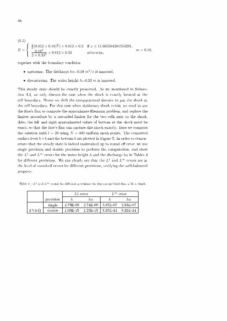
44(5.5)E =

32 (9.812 × 0.18)

23 ) + 9.812 × 0.2 if x ≤ 11.665504281554291,

0.182

2 × 0.332 + 9.812× 0.33 otherwise, m = 0.18,together with the boundary ondition• upstream: The dis harge hu=0.18 m2/s is imposed.• downstream: The water height h=0.33 m is imposed.This steady state should be exa tly preserved. As we mentioned in Subse -tion 4.3, we only dis uss the ase when the sho k is exa tly lo ated at the ell boundary. Hen e we shift the omputational domain to put the sho k atthe ell boundary. For this ase when stationary sho k exists, we need to usethe Roe's ux to ompute the approximate Riemann problem, and repla e thelimiter pro edure by a one-sided limiter for the two ells next to the sho k.Also, the left and right approximated values of bottom at the sho k must beexa t, so that the Roe's ux an apture this sho k exa tly. Here we omputethe solution until t = 20 using N = 400 uniform mesh points. The omputedsurfa e level h+b and the bottom b are plotted in Figure 3. In order to demon-strate that the steady state is indeed maintained up to round-o error, we usesingle pre ision and double pre ision to perform the omputation, and showthe L1 and L∞ errors for the water height h and the dis harge hu in Tables 4for dierent pre isions. We an learly see that the L1 and L∞ errors are atthe level of round-o errors for dierent pre isions, verifying the well-balan edproperty.Table 4 L1 and L∞ errors for dierent pre isions for the trans riti al ow with a sho k.

L1 error L∞ errorpre ision h hu h husingle 2.78E-09 2.74E-09 3.87E-07 2.53E-07FV4-Q double 1.06E-15 1.23E-15 8.37E-14 8.32E-14

45

x

surf

ace

leve

lh+

b

0 5 10 15 20 250

0.05

0.1

0.15

0.2

0.25

0.3

0.35

0.4

0.45surface level h+bbottom b

Figure 3 The surfa e level h + b and the bottom b for the trans riti al ow with a sho k. ): Sub riti al ow. The initial ondition is given by:(5.6) E = 22.06605, m = 4.42,together with the boundary ondition• upstream: The dis harge hu=4.42 m2/s is imposed.• downstream: The water height h=2 m is imposed.This steady state should be exa tly preserved. We ompute the solution until

t = 20 using N = 200 uniform mesh points. The omputed surfa e level h + band the bottom b are plotted in Figure 4. In order to demonstrate that thesteady state is indeed maintained up to round-o error, we use single pre isionand double pre ision to perform the omputation, and show the L1 and L∞errors for the water height h and the dis harge hu in Tables 5 for dierentpre isions. We an learly see that the L1 and L∞ errors are at the level ofround-o errors for dierent pre isions, verifying the well-balan ed property.

46

x

surf

ace

leve

lh+

b

0 5 10 15 20 250

0.5

1

1.5

2

2.5

surface level h+bbottom b

Figure 4 The surfa e level h + b and the bottom b for the sub riti al ow.5.2. Testing the orders of a ura yIn this example we will test the high-order a ura y of our s hemes for asmooth solution. There are some known exa t solutions to the shallow waterequation with non-at bottom in the literature, su h as some stationary so-lutions, but they are not generi test ases for a ura y. We have therefore hosen to use the following bottom fun tion and initial onditionsb(x) = sin2(πx), h(x, 0) = 5 + ecos(2πx), (hu)(x, 0) = sin(cos(2πx)), x ∈ [0, 1]Table 5 L

1 and L∞ errors for dierent pre isions for the sub riti al ow.

L1 error L∞ errorpre ision h hu h husingle 4.62E-07 3.23E-07 6.81E-06 7.23E-06double 1.44E-17 8.84E-17 6.66E-16 1.77E-15

47with periodi boundary onditions, see [34. Sin e the exa t solution isnot known expli itly for this ase, we use the fth order nite volume WENOs heme with N = 12, 800 ells to ompute a referen e solution, and treat thisreferen e solution as the exa t solution in omputing the numeri al errors.We ompute up to t = 0.1 when the solution is still smooth (sho ks developlater in time for this problem). Tables 6 and 7 ontain the L1 errors for the ell averages for FV4-Q, FV5-D and RKDG3, and for the point values forFD5, and numeri al orders of a ura y. We an learly see that the designedorder of a ura y is a hieved. For the RKDG s heme, the TVB onstant M istaken as 32. Noti e that the CFL number we have used for the nite volumes heme de reases with the mesh size and is re orded in Tables 6 and 7. Forthe RKDG method, the CFL number is xed at 0.18. We note that fth-ordera ura y is observed for FV4-Q. The fth-order WENO re onstru tion has beenused in spa e, but the sour e term is approximated by a fourth order a urateextrapolation. Hen e the approximation of the sour e term in the algorithm ontributes less to the overall error. This phenomena has been investigated in[23.5.3. A small perturbation of a steady-state waterThe following test ases are hosen to demonstrate the apability of the pro-posed s hemes for omputations on the perturbation of a steady state solution,whi h annot be aptured well by a non well-balan ed s heme. For the samereason as in Se tion 5.1, two test ases are proposed for dierent algorithms.5.3.1. Perturbation of a lake at restThe following quasi-stationary test ase was proposed by LeVeque [19. It was hosen to demonstrate the apability of the proposed s heme for omputationson a rapidly varying ow over a smooth bed, and the perturbation of a sta-tionary state. We test it on FV5-D, FD5 and RKDG3 methods.The bottom topography onsists of one hump:(5.7) b(x) =

0.25(cos(10π(x − 1.5)) + 1) if 1.4 ≤ x ≤ 1.6,

0 otherwise,

48 Table 6 L1 errors and numeri al orders of a ura y for the example in Se tion 5.2.FV4-QNo. of CFL h hu ells L1 error order L1 error order25 0.6 1.48E-02 9.78E-0250 0.6 2.41E-03 2.68 1.97E-02 2.31100 0.4 2.97E-04 3.02 2.58E-03 2.93200 0.3 2.44E-05 3.61 2.13E-04 3.60400 0.2 1.03E-06 4.56 8.97E-06 4.57800 0.1 3.49E-08 4.89 2.95E-07 4.93FV5-DCFL h hu

L1 error order L1 error order25 0.6 1.48E-02 9.45E-0250 0.6 2.40E-03 2.63 1.98E-02 2.26100 0.4 2.97E-04 3.01 2.58E-03 2.93200 0.3 2.43E-05 3.61 2.13E-04 3.60400 0.2 1.02E-06 4.57 8.96E-06 4.57800 0.1 3.26E-08 4.97 2.85E-07 4.97The initial onditions are given with(5.8) (hu)(x, 0) = 0 and h(x, 0) =

1 − b(x) + ǫ if 1.1 ≤ x ≤ 1.2,

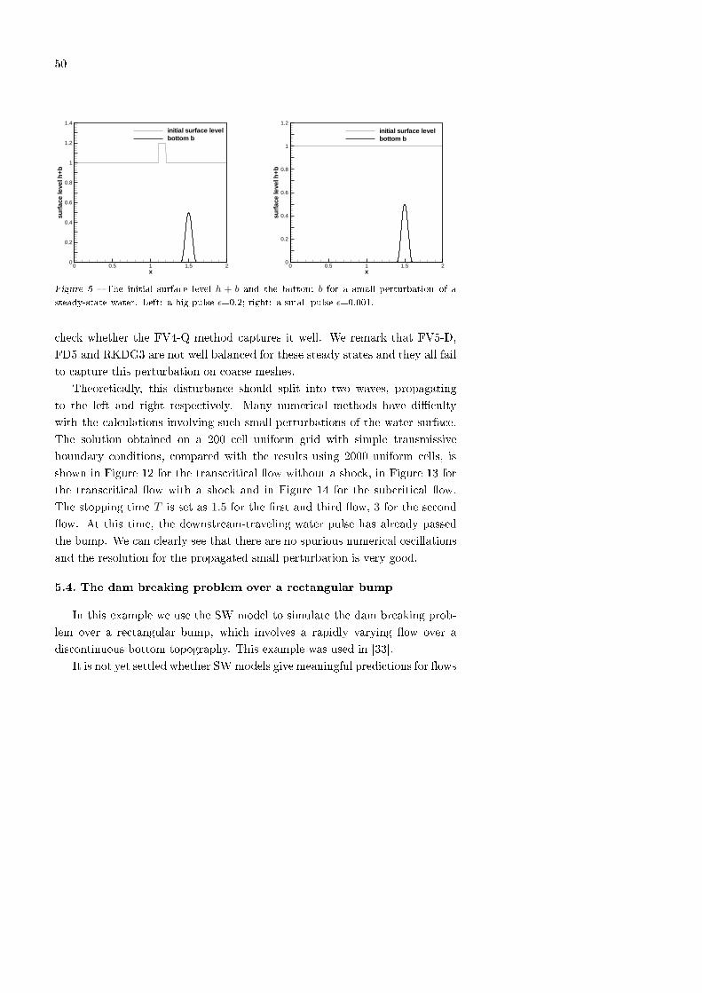
1 − b(x) otherwise,where ǫ is a non-zero perturbation onstant. Two ases have been run: ǫ =0.2 (big pulse) and ǫ = 0.001 (small pulse). Theoreti ally, for small ǫ, thisdisturban e should split into two waves, propagating left and right at the har-a teristi speeds ±√gh. Many numeri al methods have di ulty with the al ulations involving su h small perturbations of the water surfa e. Both setsof initial onditions are shown in Figure 5. The solution at time t=0.2s for thebig pulse ǫ = 0.2, obtained on a 200 ell uniform grid with simple transmissive

49Table 7 L1 errors and numeri al orders of a ura y for the example in Se tion 5.2.FD5No. of CFL h hu

L1 error order L1 error order25 0.6 1.70E-02 1.06E-0150 0.6 2.17E-03 2.97 1.95E-02 2.45100 0.6 3.33E-04 2.71 2.83E-03 2.78200 0.6 2.36E-05 3.82 2.04E-04 3.80400 0.6 9.67E-07 4.61 8.38E-06 4.61800 0.6 3.38E-08 4.84 2.94E-07 4.83RKDG3CFL h hu

L1 error order L1 error order25 0.6 2.35E-03 2.12E-0250 0.6 1.15E-04 4.36 1.01E-03 4.39100 0.4 1.24E-05 3.20 1.09E-04 3.21200 0.3 1.02E-06 3.59 8.97E-06 3.60400 0.2 1.11E-07 3.19 9.79E-07 3.19800 0.1 1.30E-08 3.09 1.14E-07 3.08boundary onditions, and ompared with a 3000 ell solution, is shown in Fig-ure 6 for the FD5, in Figure 7 for the FV5-D and in Figure 8 for the RKDG3.The results for the small pulse ǫ = 0.001 are shown in Figures 9, 10 and 11. Atthis time, the downstream-traveling water pulse has already passed the bump.We an learly see that there are no spurious numeri al os illations.5.3.2. Perturbation of steady river owIn subse tion 5.1.2, we presented three steady state solutions and showed thatour numeri al s hemes did maintain them exa tly. In this test ase, we imposeto them a small perturbation 0.01 on the height in the interval [5.75,6.25, and

50

x

surf

ace

leve

lh+

b

0 0.5 1 1.5 20

0.2

0.4

0.6

0.8

1

1.2

1.4initial surface levelbottom b

xsu

rfac

ele

velh

+b

0 0.5 1 1.5 20

0.2

0.4

0.6

0.8

1

1.2

initial surface levelbottom b

Figure 5 The initial surfa e level h + b and the bottom b for a small perturbation of asteady-state water. Left: a big pulse ǫ=0.2; right: a small pulse ǫ=0.001. he k whether the FV4-Q method aptures it well. We remark that FV5-D,FD5 and RKDG3 are not well balan ed for these steady states and they all failto apture this perturbation on oarse meshes.Theoreti ally, this disturban e should split into two waves, propagatingto the left and right respe tively. Many numeri al methods have di ultywith the al ulations involving su h small perturbations of the water surfa e.The solution obtained on a 200 ell uniform grid with simple transmissiveboundary onditions, ompared with the results using 2000 uniform ells, isshown in Figure 12 for the trans riti al ow without a sho k, in Figure 13 forthe trans riti al ow with a sho k and in Figure 14 for the sub riti al ow.The stopping time T is set as 1.5 for the rst and third ow, 3 for the se ondow. At this time, the downstream-traveling water pulse has already passedthe bump. We an learly see that there are no spurious numeri al os illationsand the resolution for the propagated small perturbation is very good.5.4. The dam breaking problem over a re tangular bumpIn this example we use the SW model to simulate the dam breaking prob-lem over a re tangular bump, whi h involves a rapidly varying ow over adis ontinuous bottom topography. This example was used in [33.It is not yet settled whether SW models give meaningful predi tions for ows

51

x

surf

ace

leve

lh+

b

0 0.5 1 1.5 20.8

0.85

0.9

0.95

1

1.05

1.1

1.15

1.2nx=3000nx=200

x

hu

0 0.5 1 1.5 2

-0.4

-0.2

0

0.2

0.4nx=3000nx=200

Figure 6 FD5: Small perturbation of a steady-state water with a big pulse. t=0.2s. Left:surfa e level h + b; right: the dis harge hu.

x

surf

ace

leve

lh+

b

0 0.5 1 1.5 20.8

0.85

0.9

0.95

1

1.05

1.1

1.15

1.2nx=3000nx=200

x

hu

0 0.5 1 1.5 2

-0.4

-0.2

0

0.2

0.4nx=3000nx=200

Figure 7 FV5-D: Small perturbation of a steady-state water with a big pulse. t=0.2s. Left:surfa e level h + b; right: the dis harge hu.

52

x

surf

ace

leve

lh+

b

0 0.5 1 1.5 20.8

0.9

1

1.1

1.2nx=3000nx=200

x

surf

ace

leve

lh+

b

0 0.5 1 1.5 2

-0.4

-0.2

0

0.2

0.4nx=3000nx=200

Figure 8 RKDG3: Small perturbation of a steady-state water with a big pulse. t=0.2s.Left: surfa e level h + b; right: the dis harge hu.

x

surf

ace

leve

lh+

b

0 0.5 1 1.5 20.999

0.9994

0.9998

1.0002

1.0006

1.001nx=3000nx=200

x

hu

0 0.5 1 1.5 2-0.002

-0.001

0

0.001

0.002nx=3000nx=200

Figure 9 FD5: Small perturbation of a steady-state water with a small pulse. t=0.2s. Left:surfa e level h + b; right: the dis harge hu.

53

x

surf

ace

leve

lh+

b

0 0.5 1 1.5 20.999

0.9994

0.9998

1.0002

1.0006

1.001nx=3000nx=200

x

hu

0 0.5 1 1.5 2-0.002

-0.001

0

0.001

0.002nx=3000nx=200

Figure 10 FV5-D: Small perturbation of a steady-state water with a small pulse. t=0.2s.Left: surfa e level h + b; right: the dis harge hu.

x

surf

ace

leve

lh+

b

0 0.5 1 1.5 20.999

0.9994

0.9998

1.0002

1.0006

1.001nx=3000nx=200

x

hu

0 0.5 1 1.5 2-0.002

-0.001

0

0.001

0.002nx=3000nx=200

Figure 11 RKDG3: Small perturbation of a steady-state water with a small pulse. t=0.2s.Left: surfa e level h + b; right: the dis harge hu.

54

x

surf

ace

leve

l,b

otto

m

0 5 10 15 20 250

0.1

0.2

0.3

0.4

0.5

0.6

0.7

0.8

0.9

1

1.1

1.2

nx=2000nx=200bottom

V1

V2

1 2 3 4 5 61.01

1.015

1.02

1.025

V1

V2

12 13 14 150.404

0.405

0.406

0.407

0.408

0.409

Figure 12 FV4-Q: Small perturbation of the trans riti al ow without a sho k.over dis ontinuous bottoms, where key modelling assumptions are violated.Should a user have to swit h to the full Euler or Navier-Stokes equations, assoon as there is a step in the bottom? The present example shows that theSW model, and our algorithms, may provide stable and sharp omputationalresults for dis ontinuous topography.The bottom topography takes the form:(5.9) b(x) =

8 if |x − 750| ≤ 1500/8,

0 otherwise,for x ∈ [0, 1500]. The initial onditions are(5.10) (hu)(x, 0) = 0 and h(x, 0) =

20 − b(x) if x ≤ 750,

15 − b(x) otherwise.

55

x

surf

ace

leve

l,b

otto

m

0 5 10 15 20 250

0.1

0.2

0.3

0.4

0.5

nx=2000nx=200bottom

V1

V2

0 0.5 1 1.5 2 2.5 30.41

0.415

0.42

0.425

V1

V2

12 12.5 13 13.5 14 14.5 15

0.326

0.328

0.33

0.332

0.334

0.336

0.338

Figure 13 FV4-Q: Small perturbation of the trans riti al ow with a sho k.Figure 15 shows numeri al results obtained by FD5 500 uniform ells (and a omparison with the results using 5000 uniform ells) with ending time t=60s.In this example, the water height h(x) is dis ontinuous at the points x=562.5and x=937.5, while the surfa e level h(x) + b(x) is smooth there. All s hemesFV4-Q, FD5, FV5-D, RKDG3 work well for this example, giving well resolved,non-os illatory solutions using 400 ells whi h agree with the onverged resultsusing 4000 ells.

56

x

surf

ace

leve

l,b

otto

m

0 5 10 15 20 250

0.5

1

1.5

2

2.5

3

nx=2000nx=200bottom

V1

V2

14 14.5 15 15.5 16 16.5 17 17.5 181.998

1.999

2

2.001

2.002

2.003

2.004

V1

V2

0 1 2 3 4 51.995

2

2.005

2.01

Figure 14 FV4-Q: Small perturbation of the sub riti al ow.5.5. A two-dimensional exampleThe shallow water system in two spa e dimensions takes the form:(5.11)

ht + (hu)x + (hv)y = 0

(hu)t +

(

hu2 +1

2gh2

)

x

+ (huv)y = −ghbx

(hv)t + (huv)x +

(

hv2 +1

2gh2

)

y

= −ghbywhere again h is the water height, (u, v) is the velo ity of the uid, b representsthe bottom topography and g is the gravitational onstant. It is straightfor-ward to generalize 1D s hemes dimension by dimension to this 2D system, andusually one will maintain the 2D well-balan ing of the lake at rest. It is also

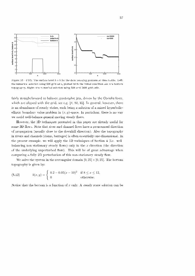
57

x

surf

ace

leve

lh+

b,bo

tto

mb

0 500 1000 15000

2

4

6

8

10

12

14

16

18

20

22h+binitial h+bbottom b

x

surf

ace

leve

lh+

b0 500 1000 1500

15

16

17

18

19

20nx=5000nx=500

Figure 15 FD5: The surfa e level h + b for the dam breaking problem at time t=60s. Left:the numeri al solution using 500 grid ells, plotted with the initial ondition and the bottomtopography; Right: the numeri al solution using 500 and 5000 grid ells.fairly straightforward to balan e geostrophi jets, driven by the Coriolis for e,whi h are aligned with the grid, see e.g. [4, 22, 25. In general, however, thereis an abundan e of steady states, ea h being a solution of a mixed hyperboli -ellipti boundary value problem in (x, y)-spa e. In parti luar, there is no waywe ould well-balan e general moving steady ows.However, the 1D te hniques presented in this paper are already useful forsome 2D ows. Note that river and hannel ows have a pronoun ed dire tionof propagation (usually lose to the downhill dire tion). Also the topographyin rivers and hannels (dams, barrages) is often essentially one-dimensional. Inthe present example, we will apply the 1D te hniques of Se tion 4 (i.e. well-balan ing non-stationary steady ows) only in the x-dire tion (the dire tionof the underlying unperturbed ow). This will be of great advantage when omputing a fully 2D perturbation of this non-stationary steady ow.We solve the system in the re tangular domain [0, 25]× [0, 25]. The bottomtopography is given by:(5.12) b(x, y) =

0.2 − 0.05(x − 10)2 if 8 ≤ x ≤ 12,

0 otherwise.Noti e that the bottom is a fun tion of x only. A steady state solution an be

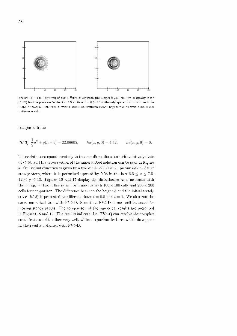
58

5 10 15 20 25

5

10

15

20

5 10 15 20 25

5

10

15

20

Figure 16 The ontours of the dieren e between the height h and the initial steady state(5.12) for the problem in Se tion 5.5 at time t = 0.5. 30 uniformly spa ed ontour lines from-0.009 to 0.012. Left: results with a 100× 100 uniform mesh. Right: results with a 200× 200uniform mesh. omputed from:(5.13) 1

2u2 + g(h + b) = 22.06605, hu(x, y, 0) = 4.42, hv(x, y, 0) = 0.These data orrespond pre isely to the one-dimensional sub riti al steady stateof (5.6), and the ross se tion of the unperturbed solution an be seen in Figure4. Our initial ondition is given by a two dimensional small perturbation of thatsteady state, where h is perturbed upward by 0.05 in the box 6.5 ≤ x ≤ 7.5,

12 ≤ y ≤ 13. Figures 16 and 17 display the disturban e as it intera ts withthe hump, on two dierent uniform meshes with 100× 100 ells and 200× 200 ells for omparison. The dieren e between the height h and the initial steadystate (5.12) is presented at dierent times t = 0.5 and t = 1. We also run thesame numeri al test with FV5-D. Note that FV5-D is not well-balan ed formoving steady states. The omparison of the numeri al results are presentedin Figures 18 and 19. The results indi ate that FV4-Q an resolve the omplexsmall features of the ow very well, without spurious features whi h do appearin the results obtained with FV5-D.

59

5 10 15 20 25

5

10

15

20

5 10 15 20 25

5

10

15

20

Figure 17 The ontours of the dieren e between the height h and the initial steady state(5.12) for the problem in Se tion 5.5 at time t = 1. 30 uniformly spa ed ontour lines from-0.005 to 0.008. Left: results with a 100× 100 uniform mesh. Right: results with a 200× 200uniform mesh.

X

0

5

10

15

20

25

Y

0

5

10

15

20

25

Heig

hth

-0.01

0

0.01

0.02

Y

X

Z

X

0

5

10

15

20

25

Y

0

5

10

15

20

25

Heig

hth

-0.01

0

0.01

0.02

Y

X

Z

Figure 18 The 3D gure of the dieren e between the height h and the initial steady state(5.12) for the problem in Se tion 5.5 at time t = 0.5 with a 200 × 200 uniform mesh. Left:results based on FV4-Q. Right: results based on FV5-D.

60X

0

5

10

15

20

25

Y

0

5

10

15

20

25

Heig

hth

-0.01

0

0.01

0.02

Y

X

Z

X

0

5

10

15

20

25

Y

0

5

10

15

20

25

Heig

hth

-0.01

0

0.01

0.02

Y

X

Z

Figure 19 The 3D gure of the dieren e between the height h and the initial steady state(5.12) for the problem in Se tion 5.5 at time t = 1 with a 200 × 200 uniform mesh. Left:results based on FV4-Q. Right: results based on FV5-D.6. ConclusionIn this paper we gave an overview of some re ently developed high-orderwell-balan ed s hemes, in luding fourth and fth order s hemes. The ex ellentresolution of the s hemes is demonstrated by a number of hallenging exper-iments for the shallow water equations. The presentation and dis ussion ofthe onstru tion prin iples should enable the reader to implement them anddevelop them further for an appli ation at hand. The onstru tions were eitherbased on well-balan ed, high-order a urate, non-os illatory nite dieren eoperators, or an well-balan ed and a urate quadrature for the regular andsingular parts of the ell-averaged residuals. The nite dieren e onstru tionmay be somewhat simpler and faster, whi h would play an even greater rolein several spa e dimensions. But the quadrature approa h an already handlemoving water steady states and is in this sense more general.References[1 E. Audusse, F. Bou hut, M.-O. Bristeau, R. Klein and B.Perthame: A fast and stable well-balan ed s heme with hydrostati re-

61 onstru tion for shallow water ows, SIAM J. S i. Comput. 25 (2004),2050-2065.[2 D.S. Bale, R.J. LeVeque, S. Mitran, and J.A. Rossmanith: Awave-propagation method for onservation laws with spatially varying uxfun tions, SIAM J. S i. Comput. 24 (2002), 955-978.[3 D.S. Balsara and C.-W. Shu: Monotoni ity preserving weighted es-sentially non-os illatory s hemes with in reasingly high order of a ura y,J. Comput. Phys. 160 (2000), 405-452.[4 F. Bou hut, J. Le Sommer and V. Zeitlin: Frontal geostrophi nonlinearwave phenomena in one dimensional rotating shallow water. Numeri alsimulations. J. Fluid Me h. 514 (2004),35-63.[5 M. Castro, J.M. Gallardo, J.A. Lopez, C. Parés: Well-balan edhigh order extensions of Godunov's method for semi-linear balan e laws,SIAM J. Num. Anal. 46 (2008), 1012-1039.[6 M. Castro, A. Pardo, C. Parés: Well-balan ed numeri al s hemesbased on a generalized hydrostati re onstru tion te hnique, Math. Mod.Meth. App. S i. (M3AS) 17 (2007), 2055-2113.[7 A. Chinnayya, A.Y. LeRoux and N. Seguin: A well-balan ed nu-meri al s heme for the approximation of the shallow-water equations withtopography: the resonan e phenomenon, Int. J. Fin. Vol. 1 (2004), ele -troni .[8 B. Co kburn: Dis ontinuous Galerkin methods for onve tion-dominated problems, in High-Order Methods for Computational Physi s,T.J. Barth and H. De onin k, editors, Le ture Notes in ComputationalS ien e and Engineering, volume 9, Springer, 1999, 69-224.[9 B. Co kburn, S.-Y. Lin and C.-W. Shu: TVB Runge-Kutta lo alproje tion dis ontinuous Galerkin nite element method for onservationlaws III: one dimensional systems, J. Comput. Phys. 84 (1989), 90-113.[10 B. Co kburn and C.-W. Shu: TVB Runge-Kutta lo al proje tion dis- ontinuous Galerkin nite element method for onservation laws II: generalframework, Math. Comp. 52 (1989), 411-435.

62[11 B. Co kburn, C.-W. Shu: The Runge-Kutta dis ontinuous Galerkinmethod for onservation laws V: Multidimensional systems, J. Comput.Phys. 141 (1998), 199-224.[12 B. Co kburn and C.-W. Shu: Runge-Kutta Dis ontinuous Galerkinmethods for onve tion-dominated problems, J. S i. Comput. 16 (2001),173-261.[13 G. Dal Maso, P. Leflo h, F. Murat: Denition and weak stabilityof non onservative produ ts, J. Math. Pures Appl. 74 (1995), 483-548.[14 L1. Gas ón and J.M. Corberán: Constru tion of se ond-order TVDs hemes for nonhomogeneous hyperboli onservation laws, J. Comput.Phys. 172 (2001), 261-297.[15 S. Gottlieb, C.-W. Shu, E. Tadmor: Strong stability-preserving high-order time dis retization methods, SIAM Rev. 43 (2001), 89-112.[16 T. Hillen: Hyperboli models for hemosensitive movement, Math. Mod.Meth. App. S i. (M3AS) 12 (2002), 1007-1034.[17 G. Jiang and C.-W. Shu: E ient implementation of weighted ENOs hemes, J. Comput. Phys. 126 (1996), 202-228.[18 A.Y. Leroux: Dis rétisation des termes sour es raides dans les problèmeshyperboliques, In Systèmes hyperboliques: noveau s hemas et nouvellesappli ations, E oles CEA-EDF-INRIA problèmes non linéaires appliqués,INRIA Ro quen ourt (Fran e), Mar h 1998. Available on http://www-gm3.univ-mrs.fr/ leroux/publi ations/ay.le_roux.html (in Fren h).[19 R.J. LeVeque: Balan ing sour e terms and ux gradients on high-resolution Godunov methods: the quasi-steady wave-propagation algo-rithm, J. Comput. Phys. 146 (1998), 346-365.[20 R. LeVeque: Finite volume methods for hyperboli problems, CambridgeTexts in Applied Mathemati s. Cambridge University Press, Cambridge,2002.[21 X.-D. Liu, S. Osher and T. Chan: Weighted essentially nonos illatorys hemes, J. Comput. Phys. 115 (1994), 200-212.

63[22 M. Luká£ová-Medvid'ová, S. Noelle and M. Kraft: Well-balan ednite volume evolution Galerkin methods for the shallow water equations,J. Comput. Phys. Vol. 221 (2007), 122-147.[23 S. Noelle, N. Pankratz, G. Puppo and J.R. Natvig: Well-balan ednite volume s hemes of arbitrary order of a ura y for shallow waterows, J. Comput. Phys. 213 (2006), 474-499.[24 S. Noelle, Y. Xing and C.-W. Shu: High order well-balan ed FiniteVolume WENO s hemes for shallow water equation with moving water, J.Comput. Phys. 226 (2007), 29-58.[25 N. Pankratz, J. Natvig, B. Gjevik and S. Noelle: High-order well-balan ed nite-volume s hemes for barotropi ows. Development and nu-meri al omparisons, O ean Mod. 18 (2007), 53-79.[26 C. Parés: Numeri al methods for non onservative hyperboli systems. Atheoreti al framework, SIAM J. Num. Anal. 44 (2006), 300-321.[27 J. Shi, C. Hu and C.-W. Shu: A te hnique of treating negative weightsin WENO s hemes, J. Comput. Phys. 175 (2002), 108-127.[28 C.-W. Shu: TVB uniformly high-order s hemes for onservation laws,Math. Comp. 49 (1987), 105-121.[29 C.-W. Shu: Total-variation-diminishing time dis retizations, SIAM J.S i. Statist. Comput. 9 (1988), 10731084.[30 C.-W. Shu: Essentially non-os illatory and weighted essentially non-os illatory s hemes for hyperboli onservation laws, in Advan ed Numer-i al Approximation of Nonlinear Hyperboli Equations, B. Co kburn, C.Johnson, C.-W. Shu and E. Tadmor (Editor: A. Quarteroni), Le tureNotes in Mathemati s, volume 1697, Springer, 1998, 325-432.[31 C.-W. Shu and S. Osher: E ient implementation of essentially non-os illatory sho k- apturing s hemes, J. Comput. Phys. 77 (1988), 439-471.[32 M.E. Vazquez-Cendon: Improved treatment of sour e terms in upwinds hemes for the shallow water equations in hannels with irregular geom-etry, J. Comput. Phys. 148 (1999), 497-526.

64[33 S. Vukovi and L. Sopta: ENO and WENO s hemes with the ex-a t onservation property for one-dimensional shallow water equations, J.Comput. Phys. 179 (2002), 593-621.[34 Y. Xing and C.-W. Shu: High order nite dieren e WENO s hemeswith the exa t onservation property for the shallow water equations, J.Comput. Phys. 208 (2005), 206-227.[35 Y. Xing and C.-W. Shu: High order well-balan ed nite dieren eWENO s hemes for a lass of hyperboli systems with sour e terms, J.S i. Comput. 27 (2006), 477-494.[36 Y. Xing and C.-W. Shu: High order well-balan ed nite volume WENOs hemes and dis ontinuous Galerkin methods for a lass of hyperboli sys-tems with sour e terms, J. Comput. Phys. 214 (2006), 567-598.[37 Y. Xing and C.-W. Shu: A new approa h of high order well-balan ednite volume WENO s hemes and dis ontinuous Galerkin methods for a lass of hyperboli systems with sour e terms, Comm. Comput. Phys. 1(2006), 100-134.