high ice water concentrations in the 19 august 2015 ... · high ice water concentrations in the 19...
TRANSCRIPT
American Institute of Aeronautics and Astronautics
1
High Ice Water Concentrations in the 19 August 2015
Coastal Mesoconvective System
Fred H Proctordagger and Steven HarrahDagger
NASA Langley Research Center Hampton VA 23681-2199
George F Switzersect Justin K Strickland and Patricia J Hunt
Analytical Mechanics Associates Inc Hampton VA 23681-2199
During August 2015 NASArsquos DC-8 research aircraft was flown into High Ice Water
Content (HIWC) events as part of a three-week campaign to collect airborne radar data and
to obtain measurements from microphysical probes Goals for this flight campaign included
improved characterization of HIWC events especially from an airborne radar perspective
This paper focuses on one of the flight days in which a coastal mesoscale convective system
(MCS) was investigated for HIWC conditions The system appears to have been maintained
by bands of convection flowing in from the Gulf of Mexico These convective bands were
capped by a large cloud canopy which masks the underlying structure if viewed from an
infrared sensing satellite The DC-8 was equipped with an IsoKinetic Probe that measured
ice concentrations of up to 23 g m-3 within the cloud canopy of this system Sustained
measurements of ice crystals with concentrations exceeding 1 g m-3 were encountered for up
to ten minutes of flight time Airborne Radar reflectivity factors were found to be weak within
these regions of high ice water concentrations suggesting that Radar detection of HIWC
would be a challenging endeavor This case is then investigated using a three-dimensional
numerical cloud model Profiles of ice water concentrations and radar reflectivity factor
demonstrate similar magnitudes and scales between the flight measurements and model
simulation Also discussed are recent modifications to the numerical modelrsquos ice-microphysics
that are based on measurements during the flight campaign The numerical model and its
updated ice-microphysics are further validated with a simulation of a well-known case of a
supercell hailstorm measured during the Cooperative Convective Precipitation Experiment
Differences in HIWC between the continental supercell and the coastal MCS are discussed
Nomenclature
AGL = Above Ground Level
BWER = Bounded Weak Echo Return
CAPE = Convective Available Potential Energy
CCOPE = Cooperative Convective Precipitation Experiment
dBZ = decibels of radar reflectivity factor Z (decibels of mm6 m-3)
Dic = ice crystal diameter (m)
DR = raindrop diameter
DS = snow particle diameter
g = acceleration due to earthrsquos gravity
|KI|2 = dielectric factor for ice (=021)
|KW|2 = dielectric factor for water (=093)
HAIC = High Altitude Ice Crystals
HIWC = High Ice Water Content
IMC = Instrumented Meteorological Conditions
dagger Senior Research Scientist Electromagnetics amp Sensors Branch MS 490 AIAA Senior Member Dagger Radar Technical Lead Electromagnetics amp Sensors Branch MS 490 sect NASA Contractor Electromagnetics amp Sensors Branch MS 490 AIAA Senior Member NASA Contractor Electromagnetics amp Sensors Branch MS 490
httpsntrsnasagovsearchjspR=20170006487 2018-07-12T164810+0000Z
American Institute of Aeronautics and Astronautics
2
IWC = ice water concentration (gm3)
MCS = Mesoscale Convection System (same as Mesoconvective Systems)
MR = mass water content for rain water (gm3)
MS = mass water content for snow water (gm3)
MSL = Mean Sea Level
N(DR) = number of raindrops per unit diameter DR per unit volume
N(DS) = number of snow particles per unit diameter DS per unit volume
NOH = intercept value in hailgraupel particle size distribution (m-4)
NOR = intercept value in raindrop size distribution (m-4)
NOS = intercept value in snow particle size distribution (m-4)
RRF = Radar Reflectivity Factor
t = time coordinate
TASS = Terminal Area Simulation System
TC = temperature (Centigrade)
xy = orthogonal space coordinates in lateral plane
V = horizontal component of velocity in y direction
z = vertical coordinate elevation
ZR = radar reflectivity factor from rain
ZS = radar reflectivity factor from snow
S = snow particle density (kg m-3)
W = specific density of water (kg m-3)
I Introduction
HE occurrence of high-concentrations of ice crystals within the upper-regions of large convective systems can
threaten the safety of commuter and large-transport jet aircraft The ingestion of ice crystals into jet engines at
large concentrations has caused uncommanded power loss including engine flameout rollback vibration and engine
damage12 Over one hundred and sixty of these engine icing incidents have been reported since the mid-1990s3 and
roughly ten incidents continue to occur internationally per year In most cases pilots have been able to restart their
engines and regain sufficient power once they have escaped the area of threat although sometimes with a significant
loss in altitude So far no known casualties or losses of aircraft have been attributed to engine icing events Another
threat from ice-crystal encounters is the obstruction of the aircraftrsquos Pitot tube which can cause erroneous
measurements of airspeed Incorrect sensing of airspeed could lead to dangerous actions from either the pilot or the
aircraftrsquos automated flight systems Similarly anomalous readings also have been reported by the aircraftrsquos total air
temperature (TAT) probes which provides temperature data for aircraft functions such as de-icing systems Typical
weather conditions during engine icing events and ice-crystal induced Pitot anomalies are subfreezing temperatures
low visibility low to moderate turbulence absence of significant airframe icing TAT anomalies static charging and
weak or no detectable radar reflectivity at flight level
Due to the international concern for air safety the detection and characterization of regions with dense ice-crystal
concentrations have been under investigation by international consortiums of airframe manufactures radar and engine
manufactures government rule making and flight operations organizations weather and aeronautical research
organizations and academia These consortiums have termed the threat of high ice-water concentrations as either
High Ice Water Content4 (HIWC) or High Altitude Ice Crystals567 (HAIC) The European-led consortiums prefer to
use HAIC to identify the aviation-hazard due to ice crystals but both acronyms are synonymous for identifying the
threat
Weather systems often associated with HIWC encounters that lead to engine icing events are large long-lasting
convective systems known as Mesoscale Convective Systems8 (MCS) (eg Fig 1) Engine icing incidents also have
occurred in the upper-levels of tropical storms as well1 Both types of systems are usually routed in oceanic or deep
moist environments that have moderate convective instability Because of the characteristic size and duration of these
weather systems9 they can inject large concentrations of ice crystals into regions near cruise altitudes10 Aircraft
incidents due to HIWC are most likely to occur with prolonged flight paths through the cloud canopies of these
systems3 Radar reflectivity factor sensed from the airborne radar usually appears innocuous due to the absence of
larger-sized ice particles Incidents due to engine icing seem less reported for flights through the anvil canopies of
supercells11 and other strong continental storms possibly due to the routine avoidance of these systems by air traffic2
These stronger continental storms will possess higher radar reflectivity even at cruise level due to hail graupel and
larger ice particles that are carried upward within strong updrafts
T
American Institute of Aeronautics and Astronautics
3
The threat of ice crystals on engine performance is dependent upon the ice crystal concentration and the duration
of exposure The actual threshold and duration necessary to induce engine power loss also may vary by engine design
and use1 Brief encounters with heavy concentrations may have little impact on engine performance compared to
prolonged exposure to moderate concentrations The certification standard for engine exposure to supercooled liquid
water is 2 g m-3 for an exposure time of 10 min12 However ice crystals may be more efficient than supercooled water
in reducing the temperature of the enginersquos internal surfaces since extra heat is absorbed by the melting of the crystals
Engine experts have suggested that an exposure to concentrations greater than about 1 g m-3 for an extended period of
time (or distance) may be sufficient to induce engine icing and power loss
Since ice water concentration is not routinely measured and is difficult to diagnose accurately from other variables
flight data is almost nonexistent for understanding relationships between ice water concentration and engine power
loss However in one incident reported by Mason et al1 an engine rollback occurred during a microphysical research
flight and therefore the power loss could be compared to the actual ice water measurement This flight was within
the low-reflectivity region downwind of a continental cumulonimbus and was exposed to ice crystals for a prolonged
period The measured ice water content peaked at 11 g m-3 and the 47 min average proceeding engine rollback was
reported as 07 g m-3 Further research is needed to define the appropriate thresholds and duration of exposure that
represent the hazard due to engine icing
II August 2015 HIWC Radar Flight Campaign
NASA along with partners including the Federal Aviation Administration (FAA) Boeing Aircraft National
Center for Atmospheric Research (NCAR) Met Analytics and Science Engineering Associates conducted a flight
campaign in August 2015 to investigate the ability of airborne weather radar to detect high concentrations of ice
crystals and to discern potentially hazardous conditions from the more benign low concentration that often exist The
flight campaign was conducted out of Fort Lauderdale Florida using NASA-Armstrongrsquos DC-8 Airborne Science
Laboratory The research aircraft was equipped with NASA-Glenn meteorological probes and NASA-Langleyrsquos
research radar The radar a modified Honeywell RDR-4000 X-band Doppler with an antenna of 4-degree beam
width was installed within the nose of the DC-8 for the flight campaign The aircraft also included equipment to
measure airspeed (Pitot tube) and total air temperature (TAT probe) as well as cloud characterization instrumentation
that included second-generation IsoKinetic Probe1314 (IKP-2) and a Robust Ice Crystal Detector (ICD)15 for
measuring ice water content Other equipment included hot-wire probes to measure water content and multiple sensors
to measure cloud and precipitation particle size distributions (precipitation imaging probe ndash PIP optical imaging -
2D-S and a cloud droplet probe ndash CDP) (Fig 2) The primary intent of this flight campaign was to further characterize
Figure 1 Mesoscale Convective System viewed from International Space Station (NASA) Overshooting tops
identify the presences of updraft plumes that feed ice crystals into the spreading cloud canopy
American Institute of Aeronautics and Astronautics
4
HIWC conditions and to investigating relationships between radar reflectivity factor ice water content and particle
size distributions
Weather information for supporting the missions was obtained from visible and infrared satellites weather station
observations ground-based weather radar and predictions from numerical weather forecast models Analysis of this
data was used to recommend time of take-off and to guide the DC-8 into potential regions with high-concentrations
of ice crystals
Ten research flights over a 20-day period were launched from Ft Lauderdale into MCS and tropical systems
Locations of these weather systems were over the Atlantic Ocean the Caribbean Sea and the Gulf of Mexico (Fig
3) Measurements during the flights were mostly over water but sometimes over inland coastal regions The DC-8
flights traversed the cloud canopies of the MCS and tropical storm convection at various elevations where ice crystals
were likely to be present Most of the data were collected at altitudes where the temperatures were colder than -25oC
For safety the most convectively-active regions of the storms were circumvented including regions with active
lightning and with flight-level radar reflectivity greater than 40 dBZ These criteria likely precluded measurements in
areas with the highest ice concentrations but these areas are usually avoided by commercial air traffic The DC-8 used
engine throttling techniques to suppress any onset of engine icing during ice crystal encounters No engine power-loss
was recorded during any of the flights
The flight campaign collected over 27 flight-hours (19600 km) of in-cloud data including long-duration exposures
to ice water concentrations greater than 1 g m-3 For each of the flight days the peak measured ice water concentration
(IWC) was greater than 2 g m-3 and the peak radar reflectivity factor (RRF) measured directly in front of the aircraftdaggerdagger
was 32 dBZ or less (Table 1) The flights through the tropical storms measured greater concentrations of ice crystal
water and at longer duration than with the flights through the oceanic and coastal MCS storms Otherwise the ice
particle distributions and the correlation between ice water content and radar reflectivity factor appeared to be similar
between each day The peak measured IWC was 32 g m-3 during a flight through tropical storm Ericka
Figure 2 NASAs DC-8 and flight campaign instrumentation including wingpods for IKP-2 and cloud particle
spectra probes fuselage-mounted instruments for background humidity water content and temperature and
a modified Honeywell RDR-4000 as primary weather radar
daggerdagger Based on criteria for RRF described above
American Institute of Aeronautics and Astronautics
5
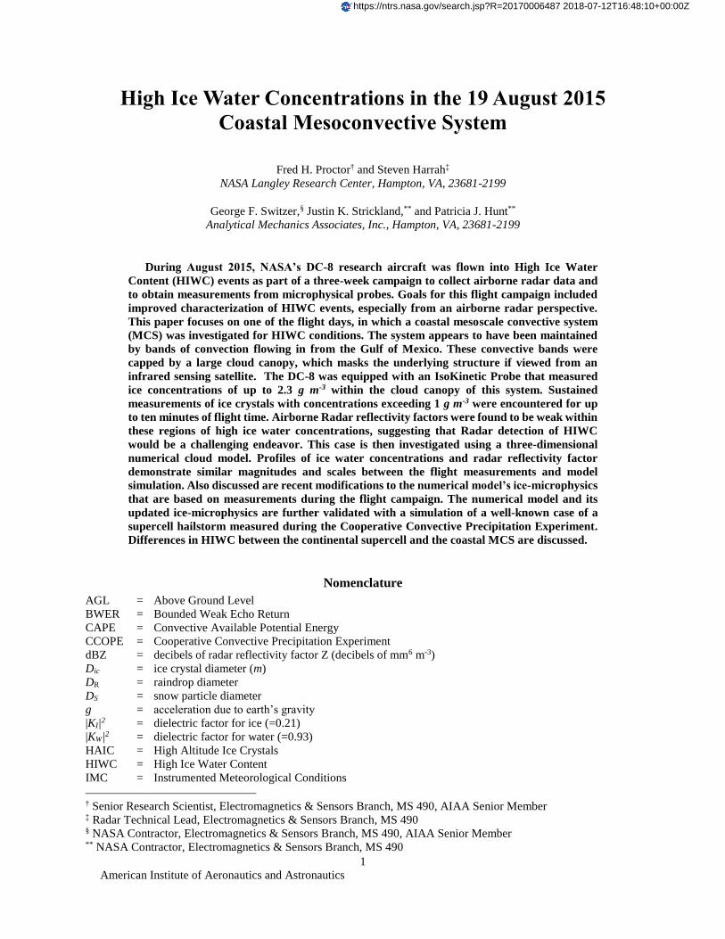
Figure 3 Depiction of the DC-8 Flight Tracks 12-28 August 2015 for NASA HIWC Radar Campaign
Table 1 Summary of flights for NASArsquos 2015 HIWC Radar Campaign
Date Max IWC
g m-3
Max Length of Path
with IWC gt
1 g m-3
Max RRF
along Trackdaggerdagger
Type of System
General Location
12 Aug 23 31 km 27 dBZ Oceanic MCS Atlantic Ocean near Southeastern US
13 Aug 23 59 km 32 dBZ Oceanic MCS Atlantic Ocean near Florida
14 Aug 27 64 km 36 dBZ Oceanic MCS Atlantic Ocean and Gulf of Mexico near Florida
16 Aug 28 186 km 30 dBZ Oceanic MCS Gulf of Mexico
19 Aug 23 114 km 28 dBZ Coastal MCS Louisiana Coast
21 Aug 27 86 km 29 dBZ Coastal MCS Louisiana Coast
23 Aug 23 139 km 27 dBZ Tropical Storm Danny
Atlantic Ocean east of Lesser Antilles
26 Aug 28 179 km 30 dBZ Tropical Storm Erika
Atlantic Ocean east of Lesser Antilles
27 Aug 32 125 km 31 dBZ Tropical Storm Erika
Caribbean Sea SE of Puerto Rico
28 Aug 29 220 km 32 dBZ Tropical Storm Erika
Caribbean Sea SW of Puerto Rico
American Institute of Aeronautics and Astronautics
6
As mentioned above no power-loss due to engine icing was noted during any of the flights however one TAT
anomaly and several Pitot tube anomalies did occur during prolonged encounters with high concentrations of ice
crystals
In section three we will summarize the observed characteristics of one of the flight days from the 2015 flight
campaign then in section five this event from this day will be examined via a numerical cloud model The numerical
cloud model the Terminal Area Simulation System (TASS) is summarized in section four In section six the same
numerical model and formulations also are applied to a benchmark case of a continental supercell hailstorm Findings
from both simulations are summarized in section seven The Appendix discusses an improved algorithm for
determining the size particle intercept for snow The relationship is derived from the August 2015 flight data and it
is applied in the numerical simulations for the coastal MCS as well as the continental supercell hailstorm
III 19 August 2015 Flight
Around 0730 UTC on 19 August a region of convection began to grow offshore of Galveston Bay Texas This
convection expanded to become a long-lasting coastal MCS that moved slowly east-northeastward along the Louisiana
coast (Figs 4 and 5) The MCS appeared to be sustained by bands of convection flowing into the system from the
Gulf and a large cloud canopy that capped the system covered much of Louisiana Developing cumulus towers
appeared to supply the southern end of these convective bands (Fig 6) Further upstream and underneath the cloud
canopy a region of steady rain fell over a wide area near the center and northern portion of the MCS
The most intense convection and the highestcoldest cloud tops were associated with the inflowing convective
bands located near the coast of Louisiana extending underneath the southern edge of the MCS cloud shield These
convective cells contained high radar reflectivity especially at low levels They also were very active with lightning
Movement of the convective cells were from the south-southwest toward the center of the MCS and new cells formed
at the southern edge to maintain the bands The lateral separation between the inflowing bans was roughly about 45
km This banded convection is evident from visible satellite but less so from infrared imagery due to partial
obscuration from the overhanging cloud canopy The MCS began to weaken after 1800 UTC as it moved through
southeastern Louisiana and into Mississippi
Figure 4 GOES Infrared Imagery for 1600 UTC 19 August 2015 Coldest cloud tops (purple ~205K) are along
the Louisiana Coast (Courtesy NASA Langley Satellite Group)
Eleven passes by the DC-8 were made through the MCS over a 4frac12-hour period (Fig 7) at elevations ranging from
29000 -37000 ft standard mean sea level (MSL) Ice crystals were encountered on these passes with sustained levels
American Institute of Aeronautics and Astronautics
7
at high concentrations measured on at least two of the passes The peak ice water content measured by IKP-2 was 23
g m-3 with the longest duration having 1 g m-3 or greater persisting over a 114 km path or during about 10 min of flight
Figure 5 Low-level radar reflectivity from NEXRAD Radar (left column) compared with visible satellite
imagery (right column) at 1600 UTC (top row) and 1645 UTC (bottom row) All four plots are of the same
spatial scale Banded convective lines are feeding into the MCS from the Gulf of Mexico
Figure 6 Lines of towering cumulus feeding into southern end of the Louisiana MCS and growing upward
through the overhanging cloud canopy Photographs from window of DC-8 courtesy of Stephanie DiVito (FAA)
American Institute of Aeronautics and Astronautics
8
Highest ice water concentrations seem to be located in the southern portion of the MCS where the convective
lines were feeding into the system The DC-8 encountered persistent regions of significant ice water concentration in
the two flight-legs along the Louisiana Coast but less so in other regions (Fig 7) Only weak concentrations were
measured in the northern regions and near the center of the cloud system where steady rain occurred
Although no engine irregularities were detected other events did happen Anomalies in airspeed due to icing of
both Pitot tube systems occurred during penetration of HIWC conditions Also during these ice crystal encounters
the DC-8 experienced 1) view of snow specks or ice particles hitting windows and being sucked into the engines 2)
IFR conditions 3) rime ice developing on both the Pitot tube and TAT probe outside the cockpit window 4) light
turbulence and 5) benign values of RRF appearing on the ship radar
This flight-day is of interest because of the storm systems structure which is unlike the MCS from the Darwin
Australia campaign that we have recently simulated10 In addition National Weather Service NEXRAD radar
(ground-based WSR-88D)16 data is available to supplement our analysis During many of the flights that were on other
days the DC-8 was not in range of ground-based radars
A scatter plot of the short-range (1micros pulse) airborne radar reflectivity factor vs measured ice water content for 19
August is shown in Fig 8 Values for IWC are measured by the IKP-2 and averaged over five seconds The criteria
for determining the RRF is that it must be detected within 1-km of the DC-8 Additionally it must be detected within
an altitude range of plusmn 150m (500 ft) of the flight path and laterally within the antenna azimuth angle of a beam width
(plusmn2 degrees) These criteria were put into place to best represent the RRF of the air that is actually encountered by the
aircraft Note that median values for RRF asymptote to near 20 dBZ when IWC increases to greater than 1 g m-3
Additionally there is a large range of scatter exists between RRF and IWC Although not shown plots from each of
the other days appear very similar having low values of RRF and a weak relationship to ice water content This would
suggest that RRF alone may be an unsuitable measurement parameter for detecting HIWC
An example from the display of the airborne research radar is shown in Fig 9 as the aircraft heads northeastward
across the Louisiana Coast This plot is sampled at a time when high ice water concentrations were being encountered
and the aircraft was passing over convective bands within the southern region of the MCS With level tilt the radar
displays mostly green (less than 30 dBZ) over a wide area Areas of higher reflectivity are evident with the downward
tilted scan and are associated with the convective bands crossing obliquely to the flight path Distinguishable radar
signatures for HIWC encounters do not seem to stand out
Figure 7 Flight path of DC-8 and measured ice water concentration from Ice Kinetic Probe for 19 August
2015
American Institute of Aeronautics and Astronautics
9
Figure 8 Peak short-range radar reflectivity factor (within 1-km of aircraft) vs ice water content measured by
IKP-2 for 19 August The median ice water concentration is represented by the red curve
Figure 9 One-hundred kilometer scan of radar reflectivity factor from the NASA Airborne Radar at 1634
UTC during HIWC encounter on 19 August for level tilt (left) and -4o tilt (right) Range rings every 5 km The
aircraft is at 885 km (29kft) MSL on an ENE baring just north of the Louisiana Coast
IV Numerical Model
A three-dimensional time-dependent numerical cloud model is used to investigate and shed further light on the
characteristic of this HIWC producing storm system Numerical simulations are performed with NASArsquos Terminal
Area Simulation System (TASS)171819 which has a history of being used to study microburst windshear 20212223
convection induced turbulence2425 aircraft wake vortices26272829 atmospheric boundary layer turbulence303132
tornadoes33 and severe convection34 Recently it has been applied to the study of HIWC such as a MCS convective
line observed during a HAIC-HIWC flight campaign at Darwin Australia10 The numerical model has prognostic
equations for velocity potential temperature pressure and water substances (water vapor cloud droplet water rain
water cloud ice crystal water snow and hailgraupel) TASS also has over 60 cloud microphysical submodels for
cloud and precipitation development The TASS formulation includes all three-phases of latent heat exchanges for
water and has a subgrid-turbulence closure formulation based on Vreman35 Boundary conditions can be periodic
American Institute of Aeronautics and Astronautics
10
open or closed and in combination The surface boundary is assumed flat and can represent either ocean or a flat
ground The impermeable surface boundary is nonslip with a parameterization for surface stress based on Monin-
Obukhov similarity theory36 Initiation packages are available for triggering cumulus convective systems turbulence
microbursts and aircraft wake vortices A summary of the salient characteristics of TASS are in Table 2 The TASS
model has over a 30-year history of supporting NASA programs37
Table 2 Salient Features in TASS
Ambient conditions initialized with atmospheric sounding
Arakawa C-grid staggered numerical mesh
Bulk parametrizations for cloud microphysics (over 60 sub-models)
Compressible time-split formulation
Efficient and accurate conservative numerical schemes with little or no numerical diffusion
Ground-stress based on Monin Obukhov Similarity Theory
History of application to aviation weather and safety problems
Initialization packages for convective storms microbursts turbulence planetary boundary layer and aircraft wake vortices
Large Eddy Simulation with subgrid scale turbulence closure
Liquid vapor and ice phase microphysics
Massively parallel interface scales efficiently with multiple processors as used on high-performance supercomputer clusters
Meteorological framework
Model simulations validated with field data and theoretical solutions
Monotone upstream-centered schemes for water substance
NonBousssinesq equation set
Nonreflective boundary conditions for open boundaries
Option of either open or periodic lateral boundaries
Option for either periodic or impermeable top and bottom boundaries
Prognostic equations for velocity pressure potential temperature dustinsects and water substance
Storm-tracking movable grid domain
Variable time step to ensure CFL criteria for numerical stability
Vreman subgrid turbulence closure model with modification for stratification and flow rotation
Water substance represented by water vapor liquid cloud water rain cloud ice snow and hailgraupel
Wet and dry growth for hail and snow
A Numerical Approximations
The TASS model equations are discretized using quadratic-conservative fourth-order finite-differences in space
for the calculation of momentum and pressure fields38 and the third-order upstream-biased Leonard scheme39 is used
to calculate the transport of potential temperature and water vapor A Monotone Upstream-centered Scheme for
Conservation Laws (MUSCL)-type scheme after van Leer4041 is used for the transport of water substance variables
Such a scheme is mostly free of negative water production from numerical error The Klemp-Wilhelmson time-
splitting scheme42 is used for computational efficiency in which the higher-frequency terms are integrated by
enforcing the CFL criteria to take into account sound wave propagation due to compressibility effects The remaining
terms are integrated using a larger time step that would be appropriate for anelastic and incompressible flows The
Adams-Bashforth scheme is assumed for time differencing of momentum and pressure for both large and small time
American Institute of Aeronautics and Astronautics
11
step approximations The TASS model is programmed in FORTRAN and operates efficiently on massively-parallel
computer architectures using Message Passing Interface (MPI) library calls
The numerics in TASS are very accurate highly efficient and nondissipative The integrity and accuracy of the
numerical and core dynamics is evaluated by performing a number of validation tests These include validation of
numerical simulations with special cases for analytical and existing high-order numerical solutions such as Beltrami
flow4344 compressible Taylor-Green Vortex454647 solutions and other test cases48 TASS has been found to achieve
high accuracy and efficient timing in these comparison tests Furthermore to ensure continued accuracy and fidelity
simulations from TASS are performed and evaluated against several baseline cases following any modification to
either the software or operating system These tests are designed to test most components and maintain efficiency
robustness and accuracy of the model
B Cloud Microphysics
TASS has over 60 bulk cloud microphysical submodels similar to those used by Lin et al49 and Rutledge and
Hobbs50 The autoconversion of cloud droplets into rain is based on drop growth studies by Berry and Reinhardt5152
and allows for differences in cloud droplet sizes usually found between continental and maritime locations17 Rain is
assumed to have an inverse-exponential drop distribution with an intercept that increases with rainwater
concentration53 in accordance with data measured by Sekhon and Srivastava54
The prediction of ice particles are divided into three different categories 1) ice crystal water mdash which represents
small hexagonal ice crystals 2) Snow mdash which represents larger precipitating ice particles and 3) hail (or graupel)
mdash which represents even larger more dense particles that are produced from freezing rain drops and riming snow
particles The ice crystal water is assumed to have a monodispersed particle size that is limited to diameters no greater
than about 200 microm These particles are represented by hexagonal plates have little fall velocity and grow primarily
by diffusion of vapor The snow category assumes spherical particles that have an inverse exponential size distribution
The size distribution intercept for snow Nos increases with decreasing temperature and snow water content The
relationship for Nos is developed from particle size distribution (PSD) data collected during the 2015 Florida flight
campaign and is described with more detail in the Appendix A category for hail and graupel particles also assume
an inverse exponential size distribution but with a smaller intercept and a larger particle density than for snow Wet
and dry growth for hail follows the formulation in Musil55 Several of the key parameters assumed for the particle
distributions are summarized in Table 3
Radar reflectivity factor is diagnosed in TASS based on the predicted water content and the assumed particle
distributions These relationships for RRF use the same particle distributions that are assumed in the microphysical
submodels The approach assumes Rayleigh scattering and is based on Smith et al56 For example the radar reflectivity
factor for rain is
119937119929 = int 119925(119915119929)infin
120782119915119929120788119941119915119929
The particle size distribution can be effectively represented by an inverse exponential distribution as
119925(119915119929) = 119925120782119929119942minus120640119915119929
where NOR is the intercept of the drop size distribution and λ is the slope The contribution of radar reflectivity factor
from rainwater can be determined with the relationship for NoR as assumed in deriving the microphysics used in TASS
(Table 3)
ZR [ mm6m3] = 94 x 103 Mr1468
where spherical drops are assumed and Mr is the rainwater content in g m-3 The radar reflectivity factor for ice particles consider the dielectric factors for ice and water and depend upon
whether the particle is undergoing either wet or dry growth For example the contribution to radar reflectivity factor
for ldquodryrdquo snow adjust for the melted diameters is
119937119930 =|119922119920|
120784
|119922119934|120784 120633119930120784
120633119960120784 int 119925(119915119930)
infin
120782119915119930120788119941119915119930 (1)
American Institute of Aeronautics and Astronautics
12
The values assumed for the dielectric factors are for wavelengths employed in weather Radars57 The contribution to
RRF from hailgraupel ice crystals and cloud droplets are computed similarly For ldquowetrdquo hail the contribution is
adjusted for Mie scattering as in Smith et al56
Table 3 Key relationships and assumptions in TASS Microphysics
Category Size Distribution and
Intercept (m-4)
Particle Density ( )
Comment
Liquid Cloud Water
Monodispersed
1000 kg m-3
NCD number of droplets per volume is an input
Rain Inverse exponential
NOR = 225 x 107 M
R
0375
1000 kg m-3
Intercept increases with rainwater content
MR (g m
-3)
Cloud Ice Crystal Water
Monodispersed
Particle mass (kg) =
01758 Dic
22
Hexagonal plates Diameter mostly lt 200 microm
Snow Inverse exponential
NOS = 10(744 ndash 00217 Tc+ X)
where
X = Ms [1053-M
s (015-
0004Ms )]
for 4oC gt Tc gt -55
oC
100 kg m-3
if
Tc lt -12 oC
Ramping to 150 kg m-3
at
Tc gt 0 oC
Intercept increases with decreasing temperature
and increasing snow
concentration Ms (g m
-3)
HailGraupel Inverse exponential Intercept is an input
parameter
Either 450 kg m-3
if graupel or
900 kg m-3
if hail
Intercept decreases with temperature when Tcgt 0oC
V Numerical Simulation of 19 August Case
In this section the numerical simulation from the 19 August case is presented to help better understand the
characteristics of this system Comparisons with measured data are presented to substantiate the credibility of the
numerical simulation
A Configuration
In modeling the HIWC conditions associated with this convective system an approach similar to that used in the
Darwin HIWC simulation10 is used The domain of the model simulation is defined to represent a section of the MCS
rather than the full volume surrounding the weather system Specifically the modelrsquos computational domain is
specified about one of the inflowing lines of convection (Fig 10) Periodic lateral boundary conditions are assumed
on the domain boundaries parallel to the convective line and open lateral boundary conditions assumed on the ends
This configuration allows the simulated line to interact as if identical parallel lines exist on either side This includes
the interaction of the canopy outflow with the adjacent convective lines via the periodic boundaries The domain also
is rotated 21o to align the model y-axis with the direction of the low-level shear vector This results in the model
domain being oriented along the convective line since observed convection often orients itself in a line along the low-
level shear vector
The domain size and resolution (Table 4) is chosen to simulate the physics adequately and to resolve the essential
three-dimensional scales of motion The domain width of 45 km is based on the typical distance separating the
inflowing convective lines The grid size is chosen to concentrate the model grid points into a 45km x 150km area
American Institute of Aeronautics and Astronautics
13
The assumed grid size is the same in all three
directions (150m) and is small enough to allow the
resolution of important thermally-driven scales of
motion
The atmospheric sounding used as input is
extrapolated from an operational weather forecast
model at a location just upstream from the system
This sounding (Fig 11) possess strong convective
instability and deep levels of moisture This sounding
also indicates a tropopause at 14km MSL with a
temperature of about -62oC or 211K Convective
indices58 computed from the sounding indicate strong
convective instability with a lifted index of about -6oC
and CAPE = 3400 J kg-1 The melting level is at
4900m MSL
The initial state of the numerical simulation is
horizontally homogeneous and varies vertically
according to the input sounding shown in Fig 11
Convection is initiated by an artificial thermal
impulse A cool pool of air that resides near the
surface over much of Louisiana and underneath the
MCS is ignored for the initial and boundary
conditions The boundary conditions for the ground
are representative of a smooth ocean surface with
constant temperature Other input parameters for the
simulation are representative of a tropical oceanic
environment (Table 5) The simulation is integrated
over a 4-hour period with convection occurring
through the full period In our simulations time (t) is in reference to time of initiation and values for the x and y
coordinates are in reference to the initial triggering impulse
B Results
The numerical simulation generates a long-lasting system with a convective line oriented in the direction of the
low-level shear vector of the environmental winds The cyclic (ie periodic) boundary conditions on the left and right
sides of the domain account for the effect of multiple lines including the interaction between the lines The type of
convection is multicellular11 with overshooting tops penetrating through the tropopause by about 600 m The system
produces persistent HIWC conditions at storm upper levels within an expanding cirrus shield fed from the multi-
Figure 11 Skew-T diagram representing initial
environmental profiles for 19 August 2015 case
Modified from sounding extracted from an operational
weather model forecast at 1400 UTC at location
upstream from the MCS (29N 912W)
Figure 10 Model Domain size relative to MCS
Table 4 Domain Size and Resolution
Domain Parameter Physical Dimension
Lateral dimensions (X Y) 45 km x 150 km
Vertical dimension (Z) 186 km
Lateral grid spacing 150 m
Vertical grid spacing 150 m
Computational grid ~39 x 10
6
grid points
Table 5 Initial Parameters
Cloud base height 625 m (942 mb)
Cloud droplet number density Ncd 75 droplets cm-3
HailGraupel particle size distribution intercept Noh
4 x 10⁵ m-4
American Institute of Aeronautics and Astronautics
14
cellular convection A comparison of the low-level radar reflectivity factor from the model simulation with the
observed NEXRAD reflectivity is shown in Fig 12
Figure 12 Comparison of low-level RRF between NEXRAD (left) and TASS (right) Observed NEXRAD
for Louisiana coast at 1645 UTC Simulated RRF at 4km altitude and 3hr 45min Outline of TASS domain
shown (90 km x 150 km)
Updrafts within the convective line generate precipitation and carry snow particles and ice crystals to the upper-
regions of the troposphere At upper levels the expanding outflow coalesces with the upper-level anvil outflow from
adjacent lines to form a large overhanging canopy (Fig 13) The general comparison between observations and
numerical simulation are summarized in
Table 6
Horizontal cross-sections at two
altitudes for RRF and IWC are shown in
Figs 14 and 15 The chosen altitudes
represent the two flight altitudes for the
DC-8 during each of two passes when
persistent IWC was measured The timing
of the slices are at a model time of
3hr45min (from the start of initialization)
and represent a time when the simulated
system has reached a mature state Profiles
are extracted along the dashed line shown
in the figures and are compared to that
measured by the DC-8 (Fig 16)
In Fig 14 the numerically simulated
ice water concentration (ice crystal snow
and graupel water combined) as well as the
RRF are shown at flight level 29 kft (8850 m) Peak ice water concentrations exceeding 3 g m-3 can be found within
small areas associated with the convective updraft turrets Larger areas with a width of about 40km exceeded 1 g m-3
Radar reflectivity factor values are generally less than 30dBZ and would appear green on the weather radar display of
most aircraft Locally higher values of RRF were found within the strong updraft cores that carry graupel and other
ice particles The RRF in Fig 14 does show large areas of low RRF but not as uniform as from the flight radar (cf
Fig 9) A more appropriate comparison would be between the RRF observed by the DC-8 with a simulation of its X-
band radar using the TASS fields as input
Figure 13 Simulated three-dimensional cloud surface viewed
from above and from south-southwest
American Institute of Aeronautics and Astronautics
15
Table 6 Comparison of general features between observed and numerically simulated for 19 August 2015 case
Feature Observed Simulated with TASS
Orientation of convective lines SSW-NNE with 45 km separation between lines
SSW-NNE with 45 km separation between lines
Cloud top elevation ~14-15 km 146 km
Coldest cloud top temperature ~200 K 203 K
Cell movement from 210o at 10 ms 221o at 11 ms
Direction of anvil canopy expansion from Southwest Southwest
Convective line movement from 290o at 6 ms 291o at 45 ms
System lifetime gt 10 hrs gt 4 hrs
Width of area with RRFgt20 dBZ at cruise altitudes
gt 50 km 40 km
At a slightly higher altitude (Fig 15) regions with HIWC cover smaller areas and have lower values of RRF This
is consistent with the measurements from the DC-8 which encountered shorter durations of IWC greater than 1
g m-3 and detected lower values of RRF after changing to a 5kft higher altitude on a subsequent pass through the
active regions near the Louisiana coast
Figure 16 shows a comparison of measured and model-extracted profiles for RRF and IWC The DC-8 flight
profiles relative to the MCS are shown in Fig 17 The TASS profiles are extrapolated at the two different altitudes
and headings flown by the DC-8 and are compared with values measured by the DC-8 At the lower elevation both
the TASS and DC-8 profiles indicate a nearly steady RRF of about 20-25 dBZ and IWC mostly between 1- 25 g m-3
At the higher elevations both TASS and DC-8 show consistent magnitudes of variation with the RRF varying between
0 to 20 dBZ and the IWC mostly remaining below 05 g m-3 Both profiles at the higher elevation do show a small
region where IWC approached 2 g m-3 Although peak values and duration of encounters seemed similar in magnitude
the variability of RRF and IWC appears greater in the modeled profiles
In Fig 18 vertical cross-sections of the simulated RRF and IWC fields are taken along the assumed flight path in
Fig 14 Note that large regions of IWC greater than 15 g m-3 (orange) extend over a large region along and below the
lower-altitude flight path Peak values occur between altitude ranges of 75-95 km AGL and drop off significantly
above 10 km AGL The corresponding RRF shows larger values below the melting level (around 5 km AGL) and very
weak values above 10 km MSL Also note that regions with significant IWC can extend above regions with low or no
detectable RRF near the ground
In summary a persistent coastal MCS system with HIWC is numerically simulated and its results compared with
data from the 2015 Florida Radar flight campaign The system is sustained by bands of convection inflowing from the
Gulf of Mexico and is capped by a large canopy cloud consisting of mostly ice crystals The simulation showed that
the coalescence of the expanding anvils from the convective cells resulted in a cloud canopy that may obscure the
banded structure and other low-level features from detection with satellite The model simulated cloud top elevations
and movement of cells appear similar to observations Largest concentrations of ice water were found in the simulation
between 75 and 95 km (25kft-31kft) MSL where environmental temperatures were between -19oC to -33oC The
range of elevations with the largest RRF were between the surface and 6km (20 kft) MSL The TASS-extracted profiles
compare reasonably with the measurements from DC-8 although some differences in variability were noted
American Institute of Aeronautics and Astronautics
16
Figure 14 Simulated RRF (left) and IWC (right) from TASS simulation at an altitude of 8850m (flight level
29kft) and 3hr and 45 min The TASS IWC field is the sum of all ice water (ice crystal water + snow + graupel)
Figure 15 Same as Fig 14 but at 10335m (flight level 34 kft)
American Institute of Aeronautics and Astronautics
17
Figure 16 Comparison of RRF and IWC extracted along flight profiles shown in Figs 14 and 15 (dashed
lines) with those measured by the DC-8 (solid lines) Top row at an altitude of 8850m bottom row at 10350m
Figure 17 Two of the DC-8 legs with longest duration of IWC
Track of DC-8 superimposed on 1645 UTC GOES-13 Infrared
satellite imagery (Courtesy NASA Langley Satellite Group)
American Institute of Aeronautics and Astronautics
18
Figure 18 Vertical cross sections of RRF (top) and IWC (bottom) extrapolated from the numerical
simulation along the flight profile shown in Fig 14 Vertical position of both flight paths shown by dashed line
Altitudes are AGL
The numerical simulation does not capture the region of stratified precipitation that lies downstream from the
inflowing convective lines However the DC-8 flights did not encounter regions of HIWC when they overflew this
region It appears likely that the rain in this area was produced by moisture from the dissipation of the convective cells
and the overrunning of the cool surface dome by the moist southerly air currents A next-generation simulation would
need to include the horizontal variation of temperature and wind into the simulation in order to capture these effects
VI Numerical Simulation of Continental Supercell Hailstorm
In this section the numerical simulation of a continental supercell hailstorm is presented The purpose of this
simulation is to validate the robustness of the microphysics used in TASS and better understand differences in HIWC
production between continental supercell storms and subtropical MCS convection Validation parameters include 1)
production of large hail 2) size of hail swath 3) radar bounded weak echo region 4) supercell features 5) storm
motion 6) size and intensity of quasi-steady updraft 7) size and maximum value of radar echo and 8) duration In
this simulation we will verify the validity of the simulation by comparing our solutions with observed data In
addition this case will be analyzed for its potential in producing HIWC and compared with the previous case of
summertime coastal convection
This case has been simulated in the past with one of the first versions of TASS using a relatively coarse mesh
Even at this earlier stage of TASS development the simulation was able to capture many of the stormrsquos observed
features5934
A Description of Observed Case
On 2 August 1981 a very large and severe hailstorm moved across Southeastern Montana The storm was observed
during its mature phase with ground-based Doppler radars and with research aircraft as it moved through a network
of field instruments during the Cooperative Convective Precipitation Experiment60 (CCOPE) The storm quickly
developed many classical features of a supercell hailstorm It veered to the right of the environmental winds and
persisted for over 5 hours while leaving a wide swath of hail The storm was reported to have an intense quasi-steady
updraft with cyclonic rotation a low-level radar hook echo signature a mid-level bounded weak echo region (BWER)
signature (same as radar echo vault) damaging winds a broad swath of 1-3 cm diameter hail with some sizes as large
American Institute of Aeronautics and Astronautics
19
as 10 cm a mesolow or mesocyclone with a peak pressure drop of at least 6mb and a peak RRF between 65-75
dBZ61626364 The primary updraft of the storm was reported to be over 14 km wide and was located within the BWER
A research aircraft flew within the updraft at an altitude between 6 km and 75 km MSL they found nearly adiabatic
conditions with updraft speeds greater than 50 m s-1 liquid water droplet concentrations of up to 6 g m-3 and the
absence of precipitation-sized particles65 The lack of larger particles explained the very low magnitudes of RRF within
the BWER Hail was penetrated by the research aircraft on the western edges of the updraft in association with the
high reflectivity regions Weisman et al66 reported that the storm produced at least one funnel cloud and that some
damage reports were ldquosuggestiverdquo of tornadic activity Surface wind speeds were estimated between 50 to 100 mph
(20 to 45 m s-1)63
A special rawinsonde sounding was launched near the storm (Fig 19) and indicated an environment very favorable
for intense convection Convective indices
calculated from the sounding exhibited a CAPE of
almost 3500 J kg-1 and a lifted Index of -10oC
The sounding also indicated a tropopause height
of 109 km MSL (~99 km AGL) with a
temperature of -475oC and an equilibrium level
at 198 mb (123 km MSL) with a temperature of -
517oC According to the both the sounding and
aircraft observations the cloud base temperature
and height were about 136oC and 26 km MSL
respectively63 The ground was slightly less than
1km above sea level and varied somewhat with
location The wind profile for the sounding
exhibited a strong magnitude of helicity6768 and
vertical shearing of the environmental wind High
values of both helicity and CAPE are indicative of
supercell and tornadic storm environments The
presence of dry environmental air at storm mid-
levels likely inhibited any strong tornado
formation (eg Proctor et al33)
B Configuration
In numerical modeling of this system we apply the
same version of the TASS model as in the Coastal-MCS
case Differences are only due to grid and domain
configuration boundary conditions input sounding and
several input parameters that define the continental
aspects of the cloud droplets and the hail size
distribution All are discussed below
The domain is size is defined to be 150 km x 150 km
in the horizontal and 20 km in the vertical (Table 7) An
evenly spaced grid size of 200 m is assumed Open
lateral boundaries conditions are applied at all lateral
boundaries The ground surface is assumed flat and no
terrain features are included The domain uses the
TASS modelrsquos internal tracking algorithms17 in
order to move the grid with the lateral translation of
the storm
The initial state profiles for temperature
pressure wind and humidity are horizontally
uniform but vary vertically according to the input
sounding shown in Fig 19 Values representative of
contental Great-Plains systems are assumed to for
the cloud droplet concentration and for the hail size
distribution intercept parameter (Table 8)
Figure 19 Skew-T diagram representing environment for
2 August 1981 Special sounding observed near Knowlton
MT at 2356 UTC Environmental wind hodograph
inserted at bottom left
Table 7 Domain Size and Resolution
Domain Parameter Physical Dimension
Lateral dimensions (X Y) 150 km x 150 km
Vertical dimension (Z) 20 km
Lateral grid spacing 200 m
Vertical grid spacing 200 m
Computational grid ~56 x 10
6
grid points
Table 8 Initial Parameters
Cloud base height (AGL) 1700 m (740 mb)
Cloud droplet number density Ncd 800 droplets cm-3
HailGraupel particle size distribution intercept Noh
2 x 10⁴ m-4
American Institute of Aeronautics and Astronautics
20
The major diffences between the initial conditions of this case and the coastal MCS case are that this case
represents a more continental environment with stronger vertical wind shear less moisture but greater instability
C Comparison of Simulation with Observations
The numerical simulation is initiated at time zero by introducing a thermal impulse and integrating over 4 hours
of time The simulation produces a supercell hailstorm and captures many of the features observed in the real storm
These include large hail wide hail swath funnel cloud with damaging surface wind 15 km wide quasi-steady updraft
surrounded at storm-mid-level by a radar echo vault or BWER a radar hook echo signature right-rear quadrant gust
front massive overshooting tops and a large spreading anvil As can be see in Table 9 scales and intenisties match
very well between the observed and simulated event The simulated updraft velocity at 65 km MSL of 55 m s-1 matches
the peak value measured by a research aircraft that penetrated the storm at the same level As found from the aircraft
measurments the updraft core was nearly adiabatic with little or no precipitation The model simulation as in the
observational studies found most of the hail to be on the western and nortwestern edges of the primary storm updraft
Table 9 Comparison of observations with TASS for 2 August 1981 Supercell Hailstorm
Features Observed TASS Simulated Anvil Extent Downstream from Updraft
(based on Radar Echo) gt200 km gt150 km
Anvil Extent Upstream from Updraft gt20 km gt60 km
BWER Diameter ~75 km ~8 km
BWER Vertical Extent 10 75 km MSL 12-14 km MSL
Gust Front Location SW Flank SW Flank
Peak Gust Front Wind Speed gt20 ms 25 ms
Typical Hail Diameter at Surface 1-3 cm peak median diameter 2 cm
Hail Shaft Location Relative to Center of BWER 3-4 km West 4-6 km WNW
Width of Hail Swath 20-30 km 225 km
Supercell Lifetime gt 5 hrs gt 4 hrs
Persistent Low-Level Radar Hook Echo yes Yes
Maximum Liquid Cloud Water Content 65 g m-3 55 g m-3
Surface Pressure Drop 6 mb Mesocyclone 4 mb tornado 21 mb
Peak Rainfall Accumulation 30-35 mm 25 mm
Peak Radar Reflectivity Factor 75 dBZ 726 dBZ
Storm Movement (development stage) 260 at 10 ms 250 at 12 ms
Storm Movement (supercell stage) 282 at 18 ms 280 at 16 ms
Storm Top Overshoot above EL 3-4 km 5 km
Updraft Diameter 14-17 km 15 km
Max Updraft Velocity at 65 km MSL 53 ms 55 ms
Diameter of 20 dBZ Echo at 12 km MSL 45 km 45 km
Peak Surface-Level Gusts East of Updraft gt25 ms 30 ms
Radar Echo Top 16 km MSL 18 km MSL
Tornadoes Funnel cloud sighted Yes western side of mesocyclone
Peak Surface Wind Damage F1- wind damage (estimated 33-50 ms)
56 ms
Maximum Altitude of 10 dbZ Contour in BWER 6-8 km MSL 65 km MSL
American Institute of Aeronautics and Astronautics
21
Supercell environments often produce tornadoes or familes of tornadoes and a funnel cloud with surface wind
damage was reported with this system The funnel cloud that was produced in the numerical simulation was
intermittent and dissiapted when it moved into the cooler dryer air underneath the hail and rain shafts Tornado
formation in this simulation showed similar characteristics to those studied in an earlier paper where the presence of
dry mid-level air acts to weaken or suppress tornado formaition in supercell environments33
The time evolution of the area with RRF greater than 55 dBZ at an elevation of 5 km MSL (blue) and the peak
RRF anywhere in the storm (red) is shown in Fig 20 The peak RRF from the simulation matches the observations
very well For the area with RRF greater than 55 dBZ both observation and TASS show a ramp up in the first two
hours of the stormrsquos lifetime but the
simulation shows this area to be smaller
than detected by ground-based radar
A comparison of the supercell structure
from TASS with measurements from
ground-based radar are shown in Figs 21
and 22 Two horizontal levels of RRF are
shown one at 10 km MSL and the other at 4
km MSL The TASS simulation reproduces
many of the observed features and supercell
signatures including the BWER (ie radar
echo Vault (V)) the radar hook echo and
the radar echo streamer The scale of the
area covered by each intensity of RRF are
similar between TASS and observed as
well One contrast however is that the high-
reflectivity area within the hook echo region
appears larger in the observation than in the
simulation The area of highest reflectivity
which is west and northwest of the BWER
is associated with large hail in both
observation and simulation
In Fig 23 a vertical cross-section along
x-z coordinates is taken through the middle
of the BWER Again both the simulation and observation show similar features similar intensities and similar spatial
scales The BWER or radar Vault is clearly present in the simulation and extends deep into the storm The BWER
is located within the intense storm updraft and is produced by a lack of significant precipitation-sized particles
D HIWC Characteristics in Simulated Storm
The Montana supercell with its quasi-steady large diameter and intense updraft generates large volumes of ice
crystals that are transported into the upper regions of the troposphere Increasing wind speeds with height which is a
characteristic of supercell environments quickly transports many of the ice particles downstream within a large
expanding anvil cloud Hail and larger ice particles are also carried up to high altitudes by the strong updrafts but fall
out relatively close-by due to their significant fall velocities Therefore large values of RRF can be found at storm
upper-levels within proximity to the supercell updraft The RRF drops-off with distance from the updraft as the larger
particles fall out and the remaining smaller particles are carried downstream
A graphical representation of the cloud and precipitation fields from TASS is show in Fig 24 Overshooting tops
which are above the predominant supercell updraft can penetrate several kilometers into the stratosphere A large
anvil cloud spreads mostly downstream from the overshooting tops due to the strong westerly winds beneath the
tropopause (cf Fig 9) This anvil cloud covers many square kilometers and forms a large overhang of cloud material
downstream from the storm updraft Due to the intensity of the updraft some the anvil material is transported counter
to upper-level winds and produces a forward overhang upstream from the storm updraft
The coldest cloud tops (Fig 25) are associated with the overshooting tops above the intense storm updraft Cloud
tops at temperaturesheights near the equilibrium level expand over a large area downstream from the overshooting
tops Obviously in Fig25 the anvil expands northeastward beyond the boundaries of the model domain
Figure 20 Time evolution of the maximum RRF anywhere
in the storm (red) and the cross-sectional area of reflectivity
exceeding 55 dBZ at 5km MSL (blue) Observed values from
Miller et al63(solid) compared with TASS (dashed)
American Institute of Aeronautics and Astronautics
22
Figure 22 Same as Fig 21 but RRF at an elevation of 4 km MSL Left adapted
from Millerrsquos analysis of ground based Doppler radar right from TASS at
t=3hr07min
RRF (dBZ)
Figure 21 Horizontal cross-section of Radar reflectivity factor at an altitude of
10 km MSL Left adapted from Millerrsquos analysis of ground based Doppler radar62
right from TASS at t=3hr07min Both plots windowed to 50km x 50km area with
major tick every 10 km The Radar echo Vault or BWER identified with V
Figure 23 Same as Fig 21 but RRF along vertical west-east cross-section through
BWER Left adapted from Millerrsquos analysis of ground based Doppler radar right from
TASS at t=3hr07min Altitude in km AGL with major ticks every 1km along abscissa
American Institute of Aeronautics and Astronautics
23
Very similar features for the simulated Montana supercell storm can be seen in the observed visible satellite
imagery of the actual system (Fig 26) The overshooting tops are positioned near the southern end and the anvil
expands toward the north-northeast The horizontal dimension of the observed cloud anvil compared with the cloud
top depicted in Fig 25 are nearly identical
Figure 27 shows the simulated IWC and RRF along a horizontal cross-section taken at 10km MSL (9km AGL)
The size and shape of the system represented in the cross-section is consistent with the satellite imagery in Fig 26 In
Fig 27 most of the RRF greater than 20 dBZ is confined to area within a 50 km diameter centered about the primary
updraft and BWER Values of RRF between 15-20 dBZ cover large areas downstream for the overshooting tops
Figure 27 also shows vast areas with IWC greater than 1 g m-3 In fact areas with 1 g m-3 or greater can be found at
distances of up to 50 to 100 km away from the regions with the greatest storm RRF Our simulation seems to imply
that by avoiding the high reflectivity areas by 20 nautical miles (37 km) may not be sufficient for avoiding prolonged
HIWC exposures
Figure 24 Simulated cloud and precipitation surfaces within the full TASS domain Viewed from south
Figure 25 Cloud top temperatures from TASS at 3hr75 min (left) and 3hr45min (right) simulation
time Coldest temperatures associated with overshooting tops in southwestern quadrant of figure
American Institute of Aeronautics and Astronautics
24
To further explore the structure of the simulated storm
vertical cross-sections are extracted alone lines A-B and C-D
that that appear in Fig27 These cross sections are shown in
Figs 28 and 29 They also help illustrate where HIWC
conditions may be found relative to the storm
The cross-sections through A-B (Fig 28) are taken
northeastward through the storm updraft It shows strong
reflectivity surrounding the BWER and extending to the upper
levels of the storm High levels of IWC largely composed of
hail are brought to the ground on the southwestern side of the
storm updraft and at upper-levels surrounding the updraft
Aircraft routinely avoid these areas due to their high values of
RRF More of a factor to air traffic is that significant levels of
IWC that can be found over large areas within the cloud
canopy at great distances downstream from the stormrsquos high
reflectivity regions Furthermore the RRF within the canopy
are very low and could be undetectable with many airborne
weather radars
In Fig 29 a cross section is taken orthogonal to the
direction of the shearing anvil It is taken northwestward
between C and D along the edge of the areas with significant
IWC (Fig 27) This cross-section resides at least 70 km or
more from areas with high RRF Along this cross section IWC
greater 1 g m-3 can be seen to extend for over a 100 km length
The layer has a thickness that is several kilometers thick This
layer also consist of very weak RRF (lt 20 dBZ) and
underneath has no detectable radar reflectivity or precipitation
Both cross-sections show that a layer with HIWC can extend over large distances and with very weak RRF
Beneath this layer containing HIWC precipitation was rarely apparent and radar reflectivity not detectable One visual
queue sometimes recommended to pilots for helping to identify potential HIWC conditions is the presence of strong
to moderate RRF from rain beneath regions of HIWC This queue would not apply to a supercell storm such as this
This case of a continental supercell also demonstrates that HIWC risks may not be confined to just oceanic and
coastal MCS since regions of significant IWC may extend for large distances with little RRF
VII Discussion and Conclusion
Flight data and results from numerical simulations are analyzed to better characterize the HIWC threat for aircraft
and to improve our understanding of the relationship between HIWC radar and satellite signatures Flight
measurements with airborne radar and microphysical probes suggest that RRF alone may not be adequate for the
detection of HIWC conditions This fact also is reinforced from the numerical model simulations
The numerical simulations confirm that HIWC can be produced in contrasting environments In warm moist
coastal and oceanic environments large volumes of ice crystals can be pumped into the upper-troposphere by
regenerating convective plumes associated with a long-lasting system Cloud material carried in the upper-level
outflow from these plumes coalesces to form a large overhanging canopy and contain significant concentrations of
ice crystals Perhaps due to the weaker wind shear of these environments and the duration of the systems large
concentrations may accumulate over time
Our simulation of a large continental supercell shows it to have a large persistent and nearly adiabatic updraft
that also can pump large volumes of ice crystals in to the upper troposphere Vertical windshear with strong winds
aloft (which are an ingredient in producing supercells) can act to transport ice crystals over large areas We speculate
that the increase ventilation due to environmental wind shear may dilute the peak concentrations of IWC in supercells
Figure 26 Observed visible satellite imagery
from GOES-7 Northeastern Montana 2315
UTC 2 August 1981
American Institute of Aeronautics and Astronautics
25
Figure 27 Ice water content (left) and RRF (right) from TASS at an elevation of 10km MSL and 3hr45
min) simulation time Ice water content (g m-3) is sum of ice crystal snow and hail water content Units
for RRF are (dBZ)
Figure 28 Vertical cross section along A-B in Fig 27 Top is ice water content (g m-3) and bottom is RRF
(dBZ) Altitudes are above ground level
American Institute of Aeronautics and Astronautics
26
In our study the microphysics for snow is improved by using analyzed PSD data measured during the flight
campaign A new relationship is developed that relates the exponential size-distribution intercept for ice particles with
their water content In the past the value for the intercept has been assumed constant or a function of temperature
only The new relationship is a function of snow or ice water content as well as temperature and was used to improve
the microphysical submodels in TASS
The TASS model was then applied to contrasting types of convection and compared to available observations
This comparison seemed very good and demonstrated the model could be applied robustly to convection in different
types of environments Excellent results were achieved using only simple bulk parametrizations for microphysics
suggesting that models that are more complex may not be needed depending upon application The profiles of ice
water content and RRF extracted from the simulation compared reasonably well with the measurements by the DC-8
during penetrations of the coastal MCS although some differences in variability were noted The TASS model was
also used to simulate a specific supercell hailstorm with excellent comparison to measurements in terms structure
features scales and magnitudes
The numerical studies for both cases found that regions of significant IWC could extend above regions with little
or no RRF This would imply that moderate to high radar reflectivity might not always be underneath HIWC events
Yet to be investigated is the potential for HIWC detection using a combination of sensors and sources for
information (ie satellite and other weather data) Also unexplored is the ability to detect HIWC with advanced
airborne radar tools
Appendix Ice Crystal Size Distributions
Relationships between the ice crystal size distributions temperature and ice water content are needed for the
parameterization of microphysical submodels used in TASS These relationships could be useful in other applications
such as the understanding the radar reflectivity factor (RRF) due to ice crystals Dr Alexei Korolev processed the
particle size distribution (PSD) data69 from data collected at one-Hertz intervals during the DC-8 flights from a 2D-S
probe and a particle-imaging probe (PIP) The measured data was discretized into appropriate size bins and normalized
by the width of the corresponding bin This allowed for the direct comparison of the PSD data with different size
resolutions and common theoretical drop-size distributions (eg Marshall-Palmer70) The size resolution for the 2D-S
probe was10 μm and 100 μm for the PIP The range of particle measurements extends from 15 μm to 12845 mm The
Figure 29 Same as in Fig 28 but for position C-D in Fig 27
American Institute of Aeronautics and Astronautics
27
size of irregularly shaped ice particles as estimated from particle images may be defined in several different ways
The composite PSD data used the length of the particle parallel to the photodiode array commonly called Ly
An intercept (N0) and slope (λ) parameter were found from the data by using a least-squares method to fit an
exponential distribution through the measured PSD This was repeated for all times in a flight Relationships can then
be established for N0S vs ice water content (IWC) and atmospheric temperature
Our numerical modeling effort previously employed a relationship for Nos that is a function of temperature
only1017 Recall that our snow category represents the larger ice particles (excluding graupel and hail) and assumes
an inverse exponential size distribution whereas our cloud ice category only represents the smaller ice particles with
diameters less than about 200 um Using combined data measured from each day of the NASA deployment (Table 1)
and binning according to temperature a new relationship was determined for Nos that is a function of both temperature
and snow water content Ms
Log10 (Nos) = 744 ndash 00217 Tc +10526 Ms ndash 015 Ms2 +0004 Ms3 (A-1)
for Tcgt -55OC and Ms lt 4 g m-3
where Nos has units of m-4 Ms has units of g m-3 and Tc is temperature of the environment in centigrade The
relationship was fitted from the flight data as shown in Fig A1 and produces a larger intercept value for either colder
temperatures or increasing snow water content A higher intercept value translates into a distribution with overall
smaller particles lower radar reflectivity factor and slightly slower fall velocity Other parameterized microphysical
processes are affected by the assumption for Nos these include sublimation or deposition of snow particles and other
growth processes
Note that when Ms 0 the above relationship asymptotes to a relationship suggested by Woods et al71 who
derived their relationship from analyzing ice particles in wintertime precipitation occurring in the Pacific Northwest
Based on all ice particles they found the following relationship for No
Log10 (No ) = 753 ndash 00207 Tc (A-2)
Since their measured ice water contents ranged between 003 and 030 g m-3 it would have been difficult for them to
detect any dependency of No on ice water content
As a further check to the validity Eq (A-1) we compare the observed short-range RRF with the value estimated
from the measured IWC using the assumption of an inverse exponential size distribution with Eq (1) as
ZS [mm6m3] = 390 x 108 Ms175 Nos
-075 (A-3)
where the above assumes melted spherical particles and accounts for the differences in radar dielectric constants for
ice and water
The comparisons are shown in Fig A1 and illustrates the lack of correlation of radar reflectivity with snow water
concentration for values of snow water greater than about 1 g m-3
American Institute of Aeronautics and Astronautics
28
Figure A1 Ice particle distribution intercept NoS
vs ice water content for three temperature ranges
Data points derived from PSD distributions
measured during all 2015 DC-8 Flight Campaign
flights (ie Table 1) Blue curve represents medium
value Red curve is fit using Eq (A-1)
Figure A2 Radar reflectivity factor vs ice
water content for three temperature ranges
Data points of close-range RRF measured during
all 2015 DC-8 Flight Campaign flights (ie Table
1) Blue curve represents medium value Red
curve using Eqs (A-3) and (A-1)
American Institute of Aeronautics and Astronautics
29
Acknowledgments
This research is sponsored by the Advanced Air Transport Technology Project of NASArsquos Advanced Air Vehicles
Program The authors would like to acknowledge the contributing organizations that enabled the Florida HIWC Radar
Flight Campaign the FAA Aviation Research Division and Aviation Weather Division the NASA Aviation Safety
Program the Boeing Company Met Analytics Science Engineering Associates Environment Canada the National
Center for Atmospheric Research Honeywell and Rockwell Collins The authors also would like to thank Tom
Ratvasky (NASA Glenn Research Center) and Walter Strapp (Met Analytics) for their programmatic technical and
operational support and the NASA Langley Satellite Group for providing satellite images In addition thanks to
Alexei Korolev (Environment and Climate Change Canada) for processing the PSD data from raw data collected
during the flight test The numerical simulations were conducted using the Pleiades high-performance supercomputer
cluster of the NASA Advanced Supercomputing Division
References
1Mason JG Strapp JW and Chow P ldquoThe Ice Particle Threat to Engines in Flightrdquo AIAA 2006-206 doi10251462006-
206 2Mason JG and Grzych M ldquoThe Challenges Identifying Weather Associated with Jet Engine Ice Crystal Icingrdquo SAE
International 2011-38-0094 doi1042712011-38-0094 3Bravin M Strapp JW and Mason J ldquoAn Investigation into Location and Convective Lifecycle Trends in an Ice Crystal
Icing Engine Event Databaserdquo SAE International 2015-01-2130 doi1042712015-01-2130 4Addy HE Jr and Veres JP ldquoAn Overview of NASA Engine Ice-Crystal Icingrdquo SAE International 2011-38-0017
doi1042712011-38-0017 5Grandin A Merle J-M Weber M Strapp JW Protat A and King P ldquoAIRBUS Flight Tests in High Ice Water Content
Regionsrdquo AIAA 2014-2753 doi10251462014-2753 6Protat A and Rauniyar S Kumar VV and Strapp JW ldquoOptimizing the Probability of Flying in High Ice Water Content
Conditions in the Tropics Using a Regional-Scale Climatology of Convective Cell Propertiesrdquo Journal of Applied Meteorology
and Climatology Vol 53 November 2014 pp 2438-2456 doi101175jamc-d-14-00021 7Dezitter F Grandin A Brenguier JL Hervy F Schlager H Villedieu P and Zalamansky G ldquoHAIC (High Altitude
Ice Crystals)rdquo AIAA 2013-2674 doi10251462013-2674 8Houze RA Jr ldquoMesoscale Convective Systemsrdquo Review of Geophysics Vol 42 RG4003 2004 pp 1-43
doi1010292004RG000150 9Grzych M Tritz T Mason J Bravin M and Sharpsten A ldquoStudies of Cloud Characteristics Related to Jet Engine Ice
Crystal Icing Utilizing Infrared Satellite Imagerrdquo SAE International 2015-01-2086 doi1042712015-01-2086 10Proctor FH and Switzer GF ldquoNumerical Simulation of HIWC Conditions with the Terminal Area Simulation Systemrdquo
AIAA-2016-4203 doi10251462016-4203 11Houze RA Jr Cloud Dynamics Ed Academic Press 1993 573 pp doi101002qj49712051918 12FAA ldquoTurbojet Turboprop and Turbofan Engine Induction System Icing and Ice Ingestionrdquo February 2004 Advisory
Circular 20-147 doi104271510198 13Davison CR Strapp JW Lilie L Ratvasky TP Dumont C ldquoIsokinetic TWC Evaporator Probe Calculations and
Systemic Uncertainty Analysisrdquo AIAA 2016-4060 doi10251462016-4060 14Strapp JW Lilie LE Ratvasky TP Davison C and Dumont C ldquoIsokinetic TWC Evaporator Probe Development of
the IKP2 and Performance Testing for the HAIC-HIWC Darwin 2014 and Cayenne-2015 Field Campaignsrdquo AIAA 2016-4059
doi10251462016-4059 15Lilie LE Sivo CP and Bouley DB ldquoDescription and Results for a Simple Ice Crystal Detection System for Airborne
Applicationsrdquo AIAA 2016-4058 doi10251462016-4058 16Crum TD and Alberty RL ldquoThe WSR-88D and the WSR-88D Operational Support Facilityrdquo Bulletin of the American
Meteorological Society Vol 74 No 9 1993 pp 1669-1688 doi1011751520-0477
doi1011751520-0477(1993)074lt1669TWATWOgt20CO2 17Proctor FH ldquoThe Terminal Area Simulation System Volume I Theoretical Formulationrdquo April 1987 NASA CR-4046 18Proctor FH ldquoNumerical Simulation of Wake Vortices Measured During the Idaho Falls and Memphis Field Programsrdquo
14th AIAA Applied Aerodynamic Conference Proceedings Part II June 1996 AIAA 96-2496-CP pp 943-960
doi10251461996-2496 19Proctor FH ldquoInteraction of Aircraft Wakes from Laterally Spaced Aircraftrdquo AIAA 2009-0343 doi10251462009-343 20Proctor FH ldquoNumerical Simulations of an Isolated Microburst Part I Dynamics and Structurerdquo Journal of the
Atmospheric Sciences Vol 45 pp 3137-3160 doi1011751520-0469(1988)045lt3137nsoaimgt20co2 21Proctor FH and Bowles RL ldquoThree-Dimensional Simulation of the Denver 11 July 1988 Microburst-Producing Stormrdquo
Meteorology and Atmospheric Physics Vol 49 1992 pp 107-124 doi101007bf01025403 22Proctor FH 1989 ldquoNumerical Simulations of an Isolated Microburst Part II Sensitivity Experimentsrdquo Journal of the
Atmospheric Sciences Vol 46 15 July 1989 pp 2143-2165 doi1011751520-0469(1989)046lt2143nsoaimgt20co2
American Institute of Aeronautics and Astronautics
30
23Proctor FH Bracalente EM Harrah SD Switzer GF and Britt CL ldquoSimulation of the 1994 Charlotte Microburst
with Look-Ahead Windshear Radarrdquo Preprints 27th Conference on Radar Meteorology American Meteorological Society October
1995 pp 530-532 Paper-10B-7 24Proctor FH Hamilton DW and Bowles RL ldquoNumerical Study of a Convective Turbulence Encounterrdquo AIAA 2002-
0944 doi10251462002-944 25Ahmad NN and Proctor FH ldquoLarge Eddy Simulations of Severe Convection Induced Turbulencerdquo AIAA 2011-3201
doi10251462011-3201 26Han J Lin Y-L Schowalter DG Arya SP and Proctor FH ldquoLarge Eddy Simulation of Aircraft Wake Vortices within
Homogeneous Turbulence Crow Instabilityrdquo AIAA Journal Vol 38 February 2000 pp 292-300 doi1025142956 27Proctor F 2004 report H Hamilton DW and Han J ldquoWake Vortex Transport and Decay in Ground Effect Vortex
Linking with the Groundrdquo AIAA 2000-0757 doi10251462000-757 28Proctor FH Hamilton DW Rutishauser DK and Switzer GF ldquoMeteorology and Wake Vortex Influence on American
Airlines FL-587 Accidentrdquo April 2004 NASA TM-2004-213018 29Proctor FH ldquoNumerical Study of a Long-Lived Isolated Wake Vortex in Ground Effectrdquo AIAA 2014-2469
doi10251462014-2469 30Schowalter DG DeCroix DS Lin Y-L Arya SP and Kaplan ML ldquoPlanetary Boundary Layer Simulation using
TASSrdquo April 1996 NASA CR-198325 31DeCroix DS Lin Y-L and Schowalter DG ldquoCellular Convection Embedded in the Convective Planetary Boundary
Layerrdquo Journal of Wind Engineering and Industrial Aerodynamics Vol 67 pp 387-401 doi101016s0167-6105(97)00088-3 32Ding F Arya SP Lin Y-L ldquoLarge-Eddy Simulation of the Atmospheric Boundary Layer Using a New Subgrid-Scale
Model II Weakly and Moderately Stable Casesrdquo Environmental Fluid Mechanics Vol 1 2001 pp 49-69
doi101023a1011543715591 33Proctor FH Ahmad NN and Limon Duparcmeur FM ldquoNumerical Simulation of a Tornado Generating Supercellrdquo
AIAA 3012-0557 doi10251462012-557 34Proctor FH ldquoThe Terminal Area Simulation System Volume II Verification Experimentsrdquo April 1987 NASA CR- 4047 35Vreman AW ldquoAn Eddy-Viscosity Subgrid-Scale Model for Turbulent Shear Flow Algebraic Theory and Applicationsrdquo
Physics of Fluids Vol 16 October 2004 pp 3670-3681 doi10106311785131 36Proctor FH and Han J ldquoNumerical Study of Wake Vortex Interaction with Ground Using the Terminal Area Simulation
Systemrdquo AIAA 99-0754 doi10251461999-754 37Switzer G and Proctor F ldquoTerminal Area Simulation System Userrsquos Guide ndash Version 100rdquo January 2014 NASA TM-
2014-218150 38Proctor FH ldquoNumerical Simulation of Wake Vortices Measured During the Idaho Falls and Memphis Field Programsrdquo
14th AIAA Applied Aerodynamic Conference Proceedings Part II June 1996 AIAA 96-2496-CP pp 943-960
doi10251461996-2496 39Leonard BP MacVean MK and Lock AP ldquoThe Flux-Integral Method for Multidimensional Convection and Diffusionrdquo
Applied Mathematical Modeling Vol 19 1995 pp 333-342 doi1010160307-904x(95)00017-e 40van Leer B ldquoTowards the Ultimate Conservative Difference Scheme V A Second-Order Sequel to Godunovrsquos Methodrdquo
Journal of Computational Physics Vol 32 1979 pp 101-136 doi1010160021-9991(79)90145-1 41Ahmad NN and Proctor FH ldquoAdvection of Microphysical Scalars in Terminal Area Simulation System (TASS)rdquo AIAA
2011-1004 doi10251462011-1004 42Klemp JB and Wilhelmson R ldquoThe Simulation of Three-Dimensional Convective Storm Dynamicsrdquo Journal of the
Atmospheric Sciences Vol 35 June 1978 pp 1070-1096 doi1011751520-0469(1978)035lt1070tsotdcgt20co2 43Wang CY ldquoExact Solutions of the Navier-Stokes Equations ndash The Generalized Beltrami Flows Review and Extensionrdquo
Acta Mechanica Vol 81 1990 pp 69-74 doi101007bf01174556 44Switzer GF ldquoValidation Tests of TASS for Application to 3-D Vortex Simulationsrdquo October 1996 NASA CR-4756 45Bull JR and Jameson A ldquoSimulation of the Compressible Taylor Green Vortex using High-Order Flux Reconstruction
Schemesrdquo AIAA 2014-3210 doi10251462014-3210 46Chapelier J-B Plata MDLL and Renac F ldquoInviscid and Viscous Simulations of the Taylor-Green Vortex Using a Modal
Discontinuous Galerkin Approachrdquo AIAA 2012-3073 doi10251462012-3073 47DeBonis JR ldquoSolutions of the Taylor-Green Vortex Problem Using High-Resolution Explicit Finite Difference Methodsrdquo
AIAA 2013-0382 doi10251462013-382 48Ahmad N and Proctor FH ldquoSimulation of Benchmark Cases with the Terminal Area Simulation Systemrdquo AIAA 2011-
1005 doi10251462011-1005 49Lin Y-L Farley RD and Orville HD ldquoBulk Parameterizations of the Snow Field in a Cloud Modelrdquo Journal of Climate
and Applied Meteorology Vol 32 1983 pp 1065-1092 doi1011751520-0450(1983)022lt1065bpotsfgt20co2 50Rutledge SA and Hobbs PV ldquoThe Mesoscale and Microscale Structure and Organization of Clouds and Precipitation
VIII A Model for the ldquoSeeder-Feederrdquo Process in Frontal Rainbandsrdquo Journal of the Atmospheric Sciences Vol 40 May 1983
pp 1185-1206 doi1011751520-0469(1983)040lt1185tmamsagt20co2
American Institute of Aeronautics and Astronautics
31
51Berry EX and Reinhardt RE ldquoAn Analysis of Cloud Drop Growth by Collection Part I Double Distributionsrdquo Journal
of the Atmospheric Sciences Vol 31 October 1974 pp 1814-1824 doi1011751520-0469(1974)031lt1814aaocdggt20co2 52Berry EX and Reinhardt RE ldquoAn Analysis of Cloud Drop Growth by Collection Part II Single Initial Distributionsrdquo
Journal of the Atmospheric Sciences Vol 31 October 1974 pp 1825-1831
doi1011751520-0469(1974)031lt1825aaocdggt20co2 53Proctor FH 1989 ldquoNumerical Simulations of an Isolated Microburst Part II Sensitivity Experimentsrdquo Journal of the
Atmospheric Sciences Vol 46 15 July 1989 pp 2143-2165 doi1011751520-0469(1989)046lt2143nsoaimgt20co2 54Sekhon RS and Srivastava RC ldquoDoppler Radar Observations of Drop-Size Distributions in a Thunderstormrdquo Journal of
the Atmospheric Sciences Vol 28 September 1971 pp 983-994 doi1011751520-0469(1971)028lt0983droodsgt20co2 55Musil DJ ldquoComputer Modeling of Hailstone Growth in Feeder Cloudsrdquo Journal of the Atmospheric Sciences Vol 27
1970 pp474-482 doi1011751520-0469(1970)027lt0474cmohgigt20co2 56Smith PL Jr Myers CG and Orville HD ldquoRadar Reflectivity Factor Calculations in Numerical Cloud Models using
Bulk Parameterizations of Precipitationrdquo Journal of Applied Meteorology Vol 14 September 1975 pp 1156-1165
doi1011751520-0450(1975)0143C1156rrfcin3E20co2 57Rogers RR A Short Course in Cloud Physics Pergamon Press 1976 227 pp doi101007bf00876948 58Blanchard DO ldquoAssessing the Vertical Distribution of Convective Available Potential Energyrdquo Weather and Forecasting
Vol 13 No 3 September 1998 pp 870-877 doi1011751520-0434(1998)013lt0870atvdocgt20co2 59Proctor FH 1985 ldquoThree Dimensional Simulation of the 2 August CCOPE Hailstorm with the Terminal Areas Simulation
Systemrdquo Report of the International Cloud Modelling WorkshopConference World Meteorological Organization WMP Report
No8 Technical Document WMOTD-139 September 1986 pp 227-240 60Knight CA ldquoThe Cooperative Convective Precipitation Experiment (CCOPE) 18 May -7 August 1981rdquo Bulletin of the
American Meteorological Society Vol 63 No 4 April 1982 pp 386-398
doi1011751520-0477(1982)063lt0386tccpemgt20co2 61Wade CG ldquoA Preliminary Study of an Intense Thunderstorm Which Moved Across the CCCOPE Research Network in
Southeastern Montanardquo Preprints 9th Conference on Forecasting and Analysisrdquo American Meteorological Society 1982 pp 388-
395 62Miller LJ ldquoThe CCOPE Hailstorm of 2 August 1981rdquo Report of the International Cloud Modelling WorkshopConference
World Meteorological Organization WMP Report No8 Technical Document WMOTD-139 September 1986 pp193-198 63Miller LJ Tuttle JD and Knight CA ldquoAirflow and Hail Growth in a Severe Northern High Plains Supercell ldquo Journal
of the Atmospheric Sciences Vol 45 No 4 1988 pp 736 doi1011751520-0469(1988)045lt0736aahgiagt20co2 64Wang PK ldquoMoisture Plumes Above Thunderstorm Anvils and their Contributions to Cross-Tropopause Transport of Water
Vapor in Midlatitudesrsquo Journal of Geophysical Research Vol 108 No D6 4194 2003 doi1010292002jd002581 65Musil DJ Heymsfield AJ and Smith PL ldquoMicrophysical Characteristics of a Well-Developed Weak Echo Region in a
High Plains Supercell Thunderstormrdquo Journal of Climate and Applied Meteorology Vol 25 July 1986 pp 1037-1051
doi1011751520-0450(1986)025lt1037mcoawdgt20co2 66Weisman ML Klemp J Miller LJ ldquoModeling and Doppler Analysis of the CCOPE August 2 Supercell Storm Preprints
13th Conference on Severe Local Storms American Meteorology Society 1983 pp 223226 67Davies-Jones RP Burgess D and Foster M ldquoTest of Helicity as a Tornado Forecast Parameterrdquo Preprints 16th Conf
on Severe Local Storms American Meteorological Society 1990 pp 588ndash592 68Brooks HE Doswell CA III and Cooper J ldquoOn the Environments of Tornadic and Nontornadic Mesocyclonesrdquo
Weather Forecasting Vol 9 December 1994 pp 606-618 doi1011751520-0434(1994)009lt0606oteotagt20co2 69Korolev A and Sussman B ldquoA Technique for Habit Classification of Cloud Particlesrdquo Journal of Atmospheric and
Oceanic Technology Vol 17 August 2000 pp 1048-1057 doi1011751520-0426(2000)017lt1048atfhcogt20co2 70Marshall JS and Palmer WM ldquoThe Distribution of Rain-Drops with Sizerdquo Journal of the Atmospheric Sciences Vol 5
1948 pp 179-207 doi1011751520-0469(1948)005lt0165tdorwsgt20co2 71Woods CP Stoelinga MT and Locatelli JD ldquoSize Spectra of Snow Particles Measured in Wintertime Precipitation in
the Pacific Northwestrdquo Journal of the Atmospheric Sciences Vol 65 January 2008 pp 189- 205 doi1011752007jas22431

American Institute of Aeronautics and Astronautics
2
IWC = ice water concentration (gm3)
MCS = Mesoscale Convection System (same as Mesoconvective Systems)
MR = mass water content for rain water (gm3)
MS = mass water content for snow water (gm3)
MSL = Mean Sea Level
N(DR) = number of raindrops per unit diameter DR per unit volume
N(DS) = number of snow particles per unit diameter DS per unit volume
NOH = intercept value in hailgraupel particle size distribution (m-4)
NOR = intercept value in raindrop size distribution (m-4)
NOS = intercept value in snow particle size distribution (m-4)
RRF = Radar Reflectivity Factor
t = time coordinate
TASS = Terminal Area Simulation System
TC = temperature (Centigrade)
xy = orthogonal space coordinates in lateral plane
V = horizontal component of velocity in y direction
z = vertical coordinate elevation
ZR = radar reflectivity factor from rain
ZS = radar reflectivity factor from snow
S = snow particle density (kg m-3)
W = specific density of water (kg m-3)
I Introduction
HE occurrence of high-concentrations of ice crystals within the upper-regions of large convective systems can
threaten the safety of commuter and large-transport jet aircraft The ingestion of ice crystals into jet engines at
large concentrations has caused uncommanded power loss including engine flameout rollback vibration and engine
damage12 Over one hundred and sixty of these engine icing incidents have been reported since the mid-1990s3 and
roughly ten incidents continue to occur internationally per year In most cases pilots have been able to restart their
engines and regain sufficient power once they have escaped the area of threat although sometimes with a significant
loss in altitude So far no known casualties or losses of aircraft have been attributed to engine icing events Another
threat from ice-crystal encounters is the obstruction of the aircraftrsquos Pitot tube which can cause erroneous
measurements of airspeed Incorrect sensing of airspeed could lead to dangerous actions from either the pilot or the
aircraftrsquos automated flight systems Similarly anomalous readings also have been reported by the aircraftrsquos total air
temperature (TAT) probes which provides temperature data for aircraft functions such as de-icing systems Typical
weather conditions during engine icing events and ice-crystal induced Pitot anomalies are subfreezing temperatures
low visibility low to moderate turbulence absence of significant airframe icing TAT anomalies static charging and
weak or no detectable radar reflectivity at flight level
Due to the international concern for air safety the detection and characterization of regions with dense ice-crystal
concentrations have been under investigation by international consortiums of airframe manufactures radar and engine
manufactures government rule making and flight operations organizations weather and aeronautical research
organizations and academia These consortiums have termed the threat of high ice-water concentrations as either
High Ice Water Content4 (HIWC) or High Altitude Ice Crystals567 (HAIC) The European-led consortiums prefer to
use HAIC to identify the aviation-hazard due to ice crystals but both acronyms are synonymous for identifying the
threat
Weather systems often associated with HIWC encounters that lead to engine icing events are large long-lasting
convective systems known as Mesoscale Convective Systems8 (MCS) (eg Fig 1) Engine icing incidents also have
occurred in the upper-levels of tropical storms as well1 Both types of systems are usually routed in oceanic or deep
moist environments that have moderate convective instability Because of the characteristic size and duration of these
weather systems9 they can inject large concentrations of ice crystals into regions near cruise altitudes10 Aircraft
incidents due to HIWC are most likely to occur with prolonged flight paths through the cloud canopies of these
systems3 Radar reflectivity factor sensed from the airborne radar usually appears innocuous due to the absence of
larger-sized ice particles Incidents due to engine icing seem less reported for flights through the anvil canopies of
supercells11 and other strong continental storms possibly due to the routine avoidance of these systems by air traffic2
These stronger continental storms will possess higher radar reflectivity even at cruise level due to hail graupel and
larger ice particles that are carried upward within strong updrafts
T
American Institute of Aeronautics and Astronautics
3
The threat of ice crystals on engine performance is dependent upon the ice crystal concentration and the duration
of exposure The actual threshold and duration necessary to induce engine power loss also may vary by engine design
and use1 Brief encounters with heavy concentrations may have little impact on engine performance compared to
prolonged exposure to moderate concentrations The certification standard for engine exposure to supercooled liquid
water is 2 g m-3 for an exposure time of 10 min12 However ice crystals may be more efficient than supercooled water
in reducing the temperature of the enginersquos internal surfaces since extra heat is absorbed by the melting of the crystals
Engine experts have suggested that an exposure to concentrations greater than about 1 g m-3 for an extended period of
time (or distance) may be sufficient to induce engine icing and power loss
Since ice water concentration is not routinely measured and is difficult to diagnose accurately from other variables
flight data is almost nonexistent for understanding relationships between ice water concentration and engine power
loss However in one incident reported by Mason et al1 an engine rollback occurred during a microphysical research
flight and therefore the power loss could be compared to the actual ice water measurement This flight was within
the low-reflectivity region downwind of a continental cumulonimbus and was exposed to ice crystals for a prolonged
period The measured ice water content peaked at 11 g m-3 and the 47 min average proceeding engine rollback was
reported as 07 g m-3 Further research is needed to define the appropriate thresholds and duration of exposure that
represent the hazard due to engine icing
II August 2015 HIWC Radar Flight Campaign
NASA along with partners including the Federal Aviation Administration (FAA) Boeing Aircraft National
Center for Atmospheric Research (NCAR) Met Analytics and Science Engineering Associates conducted a flight
campaign in August 2015 to investigate the ability of airborne weather radar to detect high concentrations of ice
crystals and to discern potentially hazardous conditions from the more benign low concentration that often exist The
flight campaign was conducted out of Fort Lauderdale Florida using NASA-Armstrongrsquos DC-8 Airborne Science
Laboratory The research aircraft was equipped with NASA-Glenn meteorological probes and NASA-Langleyrsquos
research radar The radar a modified Honeywell RDR-4000 X-band Doppler with an antenna of 4-degree beam
width was installed within the nose of the DC-8 for the flight campaign The aircraft also included equipment to
measure airspeed (Pitot tube) and total air temperature (TAT probe) as well as cloud characterization instrumentation
that included second-generation IsoKinetic Probe1314 (IKP-2) and a Robust Ice Crystal Detector (ICD)15 for
measuring ice water content Other equipment included hot-wire probes to measure water content and multiple sensors
to measure cloud and precipitation particle size distributions (precipitation imaging probe ndash PIP optical imaging -
2D-S and a cloud droplet probe ndash CDP) (Fig 2) The primary intent of this flight campaign was to further characterize
Figure 1 Mesoscale Convective System viewed from International Space Station (NASA) Overshooting tops
identify the presences of updraft plumes that feed ice crystals into the spreading cloud canopy
American Institute of Aeronautics and Astronautics
4
HIWC conditions and to investigating relationships between radar reflectivity factor ice water content and particle
size distributions
Weather information for supporting the missions was obtained from visible and infrared satellites weather station
observations ground-based weather radar and predictions from numerical weather forecast models Analysis of this
data was used to recommend time of take-off and to guide the DC-8 into potential regions with high-concentrations
of ice crystals
Ten research flights over a 20-day period were launched from Ft Lauderdale into MCS and tropical systems
Locations of these weather systems were over the Atlantic Ocean the Caribbean Sea and the Gulf of Mexico (Fig
3) Measurements during the flights were mostly over water but sometimes over inland coastal regions The DC-8
flights traversed the cloud canopies of the MCS and tropical storm convection at various elevations where ice crystals
were likely to be present Most of the data were collected at altitudes where the temperatures were colder than -25oC
For safety the most convectively-active regions of the storms were circumvented including regions with active
lightning and with flight-level radar reflectivity greater than 40 dBZ These criteria likely precluded measurements in
areas with the highest ice concentrations but these areas are usually avoided by commercial air traffic The DC-8 used
engine throttling techniques to suppress any onset of engine icing during ice crystal encounters No engine power-loss
was recorded during any of the flights
The flight campaign collected over 27 flight-hours (19600 km) of in-cloud data including long-duration exposures
to ice water concentrations greater than 1 g m-3 For each of the flight days the peak measured ice water concentration
(IWC) was greater than 2 g m-3 and the peak radar reflectivity factor (RRF) measured directly in front of the aircraftdaggerdagger
was 32 dBZ or less (Table 1) The flights through the tropical storms measured greater concentrations of ice crystal
water and at longer duration than with the flights through the oceanic and coastal MCS storms Otherwise the ice
particle distributions and the correlation between ice water content and radar reflectivity factor appeared to be similar
between each day The peak measured IWC was 32 g m-3 during a flight through tropical storm Ericka
Figure 2 NASAs DC-8 and flight campaign instrumentation including wingpods for IKP-2 and cloud particle
spectra probes fuselage-mounted instruments for background humidity water content and temperature and
a modified Honeywell RDR-4000 as primary weather radar
daggerdagger Based on criteria for RRF described above
American Institute of Aeronautics and Astronautics
5
Figure 3 Depiction of the DC-8 Flight Tracks 12-28 August 2015 for NASA HIWC Radar Campaign
Table 1 Summary of flights for NASArsquos 2015 HIWC Radar Campaign
Date Max IWC
g m-3
Max Length of Path
with IWC gt
1 g m-3
Max RRF
along Trackdaggerdagger
Type of System
General Location
12 Aug 23 31 km 27 dBZ Oceanic MCS Atlantic Ocean near Southeastern US
13 Aug 23 59 km 32 dBZ Oceanic MCS Atlantic Ocean near Florida
14 Aug 27 64 km 36 dBZ Oceanic MCS Atlantic Ocean and Gulf of Mexico near Florida
16 Aug 28 186 km 30 dBZ Oceanic MCS Gulf of Mexico
19 Aug 23 114 km 28 dBZ Coastal MCS Louisiana Coast
21 Aug 27 86 km 29 dBZ Coastal MCS Louisiana Coast
23 Aug 23 139 km 27 dBZ Tropical Storm Danny
Atlantic Ocean east of Lesser Antilles
26 Aug 28 179 km 30 dBZ Tropical Storm Erika
Atlantic Ocean east of Lesser Antilles
27 Aug 32 125 km 31 dBZ Tropical Storm Erika
Caribbean Sea SE of Puerto Rico
28 Aug 29 220 km 32 dBZ Tropical Storm Erika
Caribbean Sea SW of Puerto Rico
American Institute of Aeronautics and Astronautics
6
As mentioned above no power-loss due to engine icing was noted during any of the flights however one TAT
anomaly and several Pitot tube anomalies did occur during prolonged encounters with high concentrations of ice
crystals
In section three we will summarize the observed characteristics of one of the flight days from the 2015 flight
campaign then in section five this event from this day will be examined via a numerical cloud model The numerical
cloud model the Terminal Area Simulation System (TASS) is summarized in section four In section six the same
numerical model and formulations also are applied to a benchmark case of a continental supercell hailstorm Findings
from both simulations are summarized in section seven The Appendix discusses an improved algorithm for
determining the size particle intercept for snow The relationship is derived from the August 2015 flight data and it
is applied in the numerical simulations for the coastal MCS as well as the continental supercell hailstorm
III 19 August 2015 Flight
Around 0730 UTC on 19 August a region of convection began to grow offshore of Galveston Bay Texas This
convection expanded to become a long-lasting coastal MCS that moved slowly east-northeastward along the Louisiana
coast (Figs 4 and 5) The MCS appeared to be sustained by bands of convection flowing into the system from the
Gulf and a large cloud canopy that capped the system covered much of Louisiana Developing cumulus towers
appeared to supply the southern end of these convective bands (Fig 6) Further upstream and underneath the cloud
canopy a region of steady rain fell over a wide area near the center and northern portion of the MCS
The most intense convection and the highestcoldest cloud tops were associated with the inflowing convective
bands located near the coast of Louisiana extending underneath the southern edge of the MCS cloud shield These
convective cells contained high radar reflectivity especially at low levels They also were very active with lightning
Movement of the convective cells were from the south-southwest toward the center of the MCS and new cells formed
at the southern edge to maintain the bands The lateral separation between the inflowing bans was roughly about 45
km This banded convection is evident from visible satellite but less so from infrared imagery due to partial
obscuration from the overhanging cloud canopy The MCS began to weaken after 1800 UTC as it moved through
southeastern Louisiana and into Mississippi
Figure 4 GOES Infrared Imagery for 1600 UTC 19 August 2015 Coldest cloud tops (purple ~205K) are along
the Louisiana Coast (Courtesy NASA Langley Satellite Group)
Eleven passes by the DC-8 were made through the MCS over a 4frac12-hour period (Fig 7) at elevations ranging from
29000 -37000 ft standard mean sea level (MSL) Ice crystals were encountered on these passes with sustained levels
American Institute of Aeronautics and Astronautics
7
at high concentrations measured on at least two of the passes The peak ice water content measured by IKP-2 was 23
g m-3 with the longest duration having 1 g m-3 or greater persisting over a 114 km path or during about 10 min of flight
Figure 5 Low-level radar reflectivity from NEXRAD Radar (left column) compared with visible satellite
imagery (right column) at 1600 UTC (top row) and 1645 UTC (bottom row) All four plots are of the same
spatial scale Banded convective lines are feeding into the MCS from the Gulf of Mexico
Figure 6 Lines of towering cumulus feeding into southern end of the Louisiana MCS and growing upward
through the overhanging cloud canopy Photographs from window of DC-8 courtesy of Stephanie DiVito (FAA)
American Institute of Aeronautics and Astronautics
8
Highest ice water concentrations seem to be located in the southern portion of the MCS where the convective
lines were feeding into the system The DC-8 encountered persistent regions of significant ice water concentration in
the two flight-legs along the Louisiana Coast but less so in other regions (Fig 7) Only weak concentrations were
measured in the northern regions and near the center of the cloud system where steady rain occurred
Although no engine irregularities were detected other events did happen Anomalies in airspeed due to icing of
both Pitot tube systems occurred during penetration of HIWC conditions Also during these ice crystal encounters
the DC-8 experienced 1) view of snow specks or ice particles hitting windows and being sucked into the engines 2)
IFR conditions 3) rime ice developing on both the Pitot tube and TAT probe outside the cockpit window 4) light
turbulence and 5) benign values of RRF appearing on the ship radar
This flight-day is of interest because of the storm systems structure which is unlike the MCS from the Darwin
Australia campaign that we have recently simulated10 In addition National Weather Service NEXRAD radar
(ground-based WSR-88D)16 data is available to supplement our analysis During many of the flights that were on other
days the DC-8 was not in range of ground-based radars
A scatter plot of the short-range (1micros pulse) airborne radar reflectivity factor vs measured ice water content for 19
August is shown in Fig 8 Values for IWC are measured by the IKP-2 and averaged over five seconds The criteria
for determining the RRF is that it must be detected within 1-km of the DC-8 Additionally it must be detected within
an altitude range of plusmn 150m (500 ft) of the flight path and laterally within the antenna azimuth angle of a beam width
(plusmn2 degrees) These criteria were put into place to best represent the RRF of the air that is actually encountered by the
aircraft Note that median values for RRF asymptote to near 20 dBZ when IWC increases to greater than 1 g m-3
Additionally there is a large range of scatter exists between RRF and IWC Although not shown plots from each of
the other days appear very similar having low values of RRF and a weak relationship to ice water content This would
suggest that RRF alone may be an unsuitable measurement parameter for detecting HIWC
An example from the display of the airborne research radar is shown in Fig 9 as the aircraft heads northeastward
across the Louisiana Coast This plot is sampled at a time when high ice water concentrations were being encountered
and the aircraft was passing over convective bands within the southern region of the MCS With level tilt the radar
displays mostly green (less than 30 dBZ) over a wide area Areas of higher reflectivity are evident with the downward
tilted scan and are associated with the convective bands crossing obliquely to the flight path Distinguishable radar
signatures for HIWC encounters do not seem to stand out
Figure 7 Flight path of DC-8 and measured ice water concentration from Ice Kinetic Probe for 19 August
2015
American Institute of Aeronautics and Astronautics
9
Figure 8 Peak short-range radar reflectivity factor (within 1-km of aircraft) vs ice water content measured by
IKP-2 for 19 August The median ice water concentration is represented by the red curve
Figure 9 One-hundred kilometer scan of radar reflectivity factor from the NASA Airborne Radar at 1634
UTC during HIWC encounter on 19 August for level tilt (left) and -4o tilt (right) Range rings every 5 km The
aircraft is at 885 km (29kft) MSL on an ENE baring just north of the Louisiana Coast
IV Numerical Model
A three-dimensional time-dependent numerical cloud model is used to investigate and shed further light on the
characteristic of this HIWC producing storm system Numerical simulations are performed with NASArsquos Terminal
Area Simulation System (TASS)171819 which has a history of being used to study microburst windshear 20212223
convection induced turbulence2425 aircraft wake vortices26272829 atmospheric boundary layer turbulence303132
tornadoes33 and severe convection34 Recently it has been applied to the study of HIWC such as a MCS convective
line observed during a HAIC-HIWC flight campaign at Darwin Australia10 The numerical model has prognostic
equations for velocity potential temperature pressure and water substances (water vapor cloud droplet water rain
water cloud ice crystal water snow and hailgraupel) TASS also has over 60 cloud microphysical submodels for
cloud and precipitation development The TASS formulation includes all three-phases of latent heat exchanges for
water and has a subgrid-turbulence closure formulation based on Vreman35 Boundary conditions can be periodic
American Institute of Aeronautics and Astronautics
10
open or closed and in combination The surface boundary is assumed flat and can represent either ocean or a flat
ground The impermeable surface boundary is nonslip with a parameterization for surface stress based on Monin-
Obukhov similarity theory36 Initiation packages are available for triggering cumulus convective systems turbulence
microbursts and aircraft wake vortices A summary of the salient characteristics of TASS are in Table 2 The TASS
model has over a 30-year history of supporting NASA programs37
Table 2 Salient Features in TASS
Ambient conditions initialized with atmospheric sounding
Arakawa C-grid staggered numerical mesh
Bulk parametrizations for cloud microphysics (over 60 sub-models)
Compressible time-split formulation
Efficient and accurate conservative numerical schemes with little or no numerical diffusion
Ground-stress based on Monin Obukhov Similarity Theory
History of application to aviation weather and safety problems
Initialization packages for convective storms microbursts turbulence planetary boundary layer and aircraft wake vortices
Large Eddy Simulation with subgrid scale turbulence closure
Liquid vapor and ice phase microphysics
Massively parallel interface scales efficiently with multiple processors as used on high-performance supercomputer clusters
Meteorological framework
Model simulations validated with field data and theoretical solutions
Monotone upstream-centered schemes for water substance
NonBousssinesq equation set
Nonreflective boundary conditions for open boundaries
Option of either open or periodic lateral boundaries
Option for either periodic or impermeable top and bottom boundaries
Prognostic equations for velocity pressure potential temperature dustinsects and water substance
Storm-tracking movable grid domain
Variable time step to ensure CFL criteria for numerical stability
Vreman subgrid turbulence closure model with modification for stratification and flow rotation
Water substance represented by water vapor liquid cloud water rain cloud ice snow and hailgraupel
Wet and dry growth for hail and snow
A Numerical Approximations
The TASS model equations are discretized using quadratic-conservative fourth-order finite-differences in space
for the calculation of momentum and pressure fields38 and the third-order upstream-biased Leonard scheme39 is used
to calculate the transport of potential temperature and water vapor A Monotone Upstream-centered Scheme for
Conservation Laws (MUSCL)-type scheme after van Leer4041 is used for the transport of water substance variables
Such a scheme is mostly free of negative water production from numerical error The Klemp-Wilhelmson time-
splitting scheme42 is used for computational efficiency in which the higher-frequency terms are integrated by
enforcing the CFL criteria to take into account sound wave propagation due to compressibility effects The remaining
terms are integrated using a larger time step that would be appropriate for anelastic and incompressible flows The
Adams-Bashforth scheme is assumed for time differencing of momentum and pressure for both large and small time
American Institute of Aeronautics and Astronautics
11
step approximations The TASS model is programmed in FORTRAN and operates efficiently on massively-parallel
computer architectures using Message Passing Interface (MPI) library calls
The numerics in TASS are very accurate highly efficient and nondissipative The integrity and accuracy of the
numerical and core dynamics is evaluated by performing a number of validation tests These include validation of
numerical simulations with special cases for analytical and existing high-order numerical solutions such as Beltrami
flow4344 compressible Taylor-Green Vortex454647 solutions and other test cases48 TASS has been found to achieve
high accuracy and efficient timing in these comparison tests Furthermore to ensure continued accuracy and fidelity
simulations from TASS are performed and evaluated against several baseline cases following any modification to
either the software or operating system These tests are designed to test most components and maintain efficiency
robustness and accuracy of the model
B Cloud Microphysics
TASS has over 60 bulk cloud microphysical submodels similar to those used by Lin et al49 and Rutledge and
Hobbs50 The autoconversion of cloud droplets into rain is based on drop growth studies by Berry and Reinhardt5152
and allows for differences in cloud droplet sizes usually found between continental and maritime locations17 Rain is
assumed to have an inverse-exponential drop distribution with an intercept that increases with rainwater
concentration53 in accordance with data measured by Sekhon and Srivastava54
The prediction of ice particles are divided into three different categories 1) ice crystal water mdash which represents
small hexagonal ice crystals 2) Snow mdash which represents larger precipitating ice particles and 3) hail (or graupel)
mdash which represents even larger more dense particles that are produced from freezing rain drops and riming snow
particles The ice crystal water is assumed to have a monodispersed particle size that is limited to diameters no greater
than about 200 microm These particles are represented by hexagonal plates have little fall velocity and grow primarily
by diffusion of vapor The snow category assumes spherical particles that have an inverse exponential size distribution
The size distribution intercept for snow Nos increases with decreasing temperature and snow water content The
relationship for Nos is developed from particle size distribution (PSD) data collected during the 2015 Florida flight
campaign and is described with more detail in the Appendix A category for hail and graupel particles also assume
an inverse exponential size distribution but with a smaller intercept and a larger particle density than for snow Wet
and dry growth for hail follows the formulation in Musil55 Several of the key parameters assumed for the particle
distributions are summarized in Table 3
Radar reflectivity factor is diagnosed in TASS based on the predicted water content and the assumed particle
distributions These relationships for RRF use the same particle distributions that are assumed in the microphysical
submodels The approach assumes Rayleigh scattering and is based on Smith et al56 For example the radar reflectivity
factor for rain is
119937119929 = int 119925(119915119929)infin
120782119915119929120788119941119915119929
The particle size distribution can be effectively represented by an inverse exponential distribution as
119925(119915119929) = 119925120782119929119942minus120640119915119929
where NOR is the intercept of the drop size distribution and λ is the slope The contribution of radar reflectivity factor
from rainwater can be determined with the relationship for NoR as assumed in deriving the microphysics used in TASS
(Table 3)
ZR [ mm6m3] = 94 x 103 Mr1468
where spherical drops are assumed and Mr is the rainwater content in g m-3 The radar reflectivity factor for ice particles consider the dielectric factors for ice and water and depend upon
whether the particle is undergoing either wet or dry growth For example the contribution to radar reflectivity factor
for ldquodryrdquo snow adjust for the melted diameters is
119937119930 =|119922119920|
120784
|119922119934|120784 120633119930120784
120633119960120784 int 119925(119915119930)
infin
120782119915119930120788119941119915119930 (1)
American Institute of Aeronautics and Astronautics
12
The values assumed for the dielectric factors are for wavelengths employed in weather Radars57 The contribution to
RRF from hailgraupel ice crystals and cloud droplets are computed similarly For ldquowetrdquo hail the contribution is
adjusted for Mie scattering as in Smith et al56
Table 3 Key relationships and assumptions in TASS Microphysics
Category Size Distribution and
Intercept (m-4)
Particle Density ( )
Comment
Liquid Cloud Water
Monodispersed
1000 kg m-3
NCD number of droplets per volume is an input
Rain Inverse exponential
NOR = 225 x 107 M
R
0375
1000 kg m-3
Intercept increases with rainwater content
MR (g m
-3)
Cloud Ice Crystal Water
Monodispersed
Particle mass (kg) =
01758 Dic
22
Hexagonal plates Diameter mostly lt 200 microm
Snow Inverse exponential
NOS = 10(744 ndash 00217 Tc+ X)
where
X = Ms [1053-M
s (015-
0004Ms )]
for 4oC gt Tc gt -55
oC
100 kg m-3
if
Tc lt -12 oC
Ramping to 150 kg m-3
at
Tc gt 0 oC
Intercept increases with decreasing temperature
and increasing snow
concentration Ms (g m
-3)
HailGraupel Inverse exponential Intercept is an input
parameter
Either 450 kg m-3
if graupel or
900 kg m-3
if hail
Intercept decreases with temperature when Tcgt 0oC
V Numerical Simulation of 19 August Case
In this section the numerical simulation from the 19 August case is presented to help better understand the
characteristics of this system Comparisons with measured data are presented to substantiate the credibility of the
numerical simulation
A Configuration
In modeling the HIWC conditions associated with this convective system an approach similar to that used in the
Darwin HIWC simulation10 is used The domain of the model simulation is defined to represent a section of the MCS
rather than the full volume surrounding the weather system Specifically the modelrsquos computational domain is
specified about one of the inflowing lines of convection (Fig 10) Periodic lateral boundary conditions are assumed
on the domain boundaries parallel to the convective line and open lateral boundary conditions assumed on the ends
This configuration allows the simulated line to interact as if identical parallel lines exist on either side This includes
the interaction of the canopy outflow with the adjacent convective lines via the periodic boundaries The domain also
is rotated 21o to align the model y-axis with the direction of the low-level shear vector This results in the model
domain being oriented along the convective line since observed convection often orients itself in a line along the low-
level shear vector
The domain size and resolution (Table 4) is chosen to simulate the physics adequately and to resolve the essential
three-dimensional scales of motion The domain width of 45 km is based on the typical distance separating the
inflowing convective lines The grid size is chosen to concentrate the model grid points into a 45km x 150km area
American Institute of Aeronautics and Astronautics
13
The assumed grid size is the same in all three
directions (150m) and is small enough to allow the
resolution of important thermally-driven scales of
motion
The atmospheric sounding used as input is
extrapolated from an operational weather forecast
model at a location just upstream from the system
This sounding (Fig 11) possess strong convective
instability and deep levels of moisture This sounding
also indicates a tropopause at 14km MSL with a
temperature of about -62oC or 211K Convective
indices58 computed from the sounding indicate strong
convective instability with a lifted index of about -6oC
and CAPE = 3400 J kg-1 The melting level is at
4900m MSL
The initial state of the numerical simulation is
horizontally homogeneous and varies vertically
according to the input sounding shown in Fig 11
Convection is initiated by an artificial thermal
impulse A cool pool of air that resides near the
surface over much of Louisiana and underneath the
MCS is ignored for the initial and boundary
conditions The boundary conditions for the ground
are representative of a smooth ocean surface with
constant temperature Other input parameters for the
simulation are representative of a tropical oceanic
environment (Table 5) The simulation is integrated
over a 4-hour period with convection occurring
through the full period In our simulations time (t) is in reference to time of initiation and values for the x and y
coordinates are in reference to the initial triggering impulse
B Results
The numerical simulation generates a long-lasting system with a convective line oriented in the direction of the
low-level shear vector of the environmental winds The cyclic (ie periodic) boundary conditions on the left and right
sides of the domain account for the effect of multiple lines including the interaction between the lines The type of
convection is multicellular11 with overshooting tops penetrating through the tropopause by about 600 m The system
produces persistent HIWC conditions at storm upper levels within an expanding cirrus shield fed from the multi-
Figure 11 Skew-T diagram representing initial
environmental profiles for 19 August 2015 case
Modified from sounding extracted from an operational
weather model forecast at 1400 UTC at location
upstream from the MCS (29N 912W)
Figure 10 Model Domain size relative to MCS
Table 4 Domain Size and Resolution
Domain Parameter Physical Dimension
Lateral dimensions (X Y) 45 km x 150 km
Vertical dimension (Z) 186 km
Lateral grid spacing 150 m
Vertical grid spacing 150 m
Computational grid ~39 x 10
6
grid points
Table 5 Initial Parameters
Cloud base height 625 m (942 mb)
Cloud droplet number density Ncd 75 droplets cm-3
HailGraupel particle size distribution intercept Noh
4 x 10⁵ m-4
American Institute of Aeronautics and Astronautics
14
cellular convection A comparison of the low-level radar reflectivity factor from the model simulation with the
observed NEXRAD reflectivity is shown in Fig 12
Figure 12 Comparison of low-level RRF between NEXRAD (left) and TASS (right) Observed NEXRAD
for Louisiana coast at 1645 UTC Simulated RRF at 4km altitude and 3hr 45min Outline of TASS domain
shown (90 km x 150 km)
Updrafts within the convective line generate precipitation and carry snow particles and ice crystals to the upper-
regions of the troposphere At upper levels the expanding outflow coalesces with the upper-level anvil outflow from
adjacent lines to form a large overhanging canopy (Fig 13) The general comparison between observations and
numerical simulation are summarized in
Table 6
Horizontal cross-sections at two
altitudes for RRF and IWC are shown in
Figs 14 and 15 The chosen altitudes
represent the two flight altitudes for the
DC-8 during each of two passes when
persistent IWC was measured The timing
of the slices are at a model time of
3hr45min (from the start of initialization)
and represent a time when the simulated
system has reached a mature state Profiles
are extracted along the dashed line shown
in the figures and are compared to that
measured by the DC-8 (Fig 16)
In Fig 14 the numerically simulated
ice water concentration (ice crystal snow
and graupel water combined) as well as the
RRF are shown at flight level 29 kft (8850 m) Peak ice water concentrations exceeding 3 g m-3 can be found within
small areas associated with the convective updraft turrets Larger areas with a width of about 40km exceeded 1 g m-3
Radar reflectivity factor values are generally less than 30dBZ and would appear green on the weather radar display of
most aircraft Locally higher values of RRF were found within the strong updraft cores that carry graupel and other
ice particles The RRF in Fig 14 does show large areas of low RRF but not as uniform as from the flight radar (cf
Fig 9) A more appropriate comparison would be between the RRF observed by the DC-8 with a simulation of its X-
band radar using the TASS fields as input
Figure 13 Simulated three-dimensional cloud surface viewed
from above and from south-southwest
American Institute of Aeronautics and Astronautics
15
Table 6 Comparison of general features between observed and numerically simulated for 19 August 2015 case
Feature Observed Simulated with TASS
Orientation of convective lines SSW-NNE with 45 km separation between lines
SSW-NNE with 45 km separation between lines
Cloud top elevation ~14-15 km 146 km
Coldest cloud top temperature ~200 K 203 K
Cell movement from 210o at 10 ms 221o at 11 ms
Direction of anvil canopy expansion from Southwest Southwest
Convective line movement from 290o at 6 ms 291o at 45 ms
System lifetime gt 10 hrs gt 4 hrs
Width of area with RRFgt20 dBZ at cruise altitudes
gt 50 km 40 km
At a slightly higher altitude (Fig 15) regions with HIWC cover smaller areas and have lower values of RRF This
is consistent with the measurements from the DC-8 which encountered shorter durations of IWC greater than 1
g m-3 and detected lower values of RRF after changing to a 5kft higher altitude on a subsequent pass through the
active regions near the Louisiana coast
Figure 16 shows a comparison of measured and model-extracted profiles for RRF and IWC The DC-8 flight
profiles relative to the MCS are shown in Fig 17 The TASS profiles are extrapolated at the two different altitudes
and headings flown by the DC-8 and are compared with values measured by the DC-8 At the lower elevation both
the TASS and DC-8 profiles indicate a nearly steady RRF of about 20-25 dBZ and IWC mostly between 1- 25 g m-3
At the higher elevations both TASS and DC-8 show consistent magnitudes of variation with the RRF varying between
0 to 20 dBZ and the IWC mostly remaining below 05 g m-3 Both profiles at the higher elevation do show a small
region where IWC approached 2 g m-3 Although peak values and duration of encounters seemed similar in magnitude
the variability of RRF and IWC appears greater in the modeled profiles
In Fig 18 vertical cross-sections of the simulated RRF and IWC fields are taken along the assumed flight path in
Fig 14 Note that large regions of IWC greater than 15 g m-3 (orange) extend over a large region along and below the
lower-altitude flight path Peak values occur between altitude ranges of 75-95 km AGL and drop off significantly
above 10 km AGL The corresponding RRF shows larger values below the melting level (around 5 km AGL) and very
weak values above 10 km MSL Also note that regions with significant IWC can extend above regions with low or no
detectable RRF near the ground
In summary a persistent coastal MCS system with HIWC is numerically simulated and its results compared with
data from the 2015 Florida Radar flight campaign The system is sustained by bands of convection inflowing from the
Gulf of Mexico and is capped by a large canopy cloud consisting of mostly ice crystals The simulation showed that
the coalescence of the expanding anvils from the convective cells resulted in a cloud canopy that may obscure the
banded structure and other low-level features from detection with satellite The model simulated cloud top elevations
and movement of cells appear similar to observations Largest concentrations of ice water were found in the simulation
between 75 and 95 km (25kft-31kft) MSL where environmental temperatures were between -19oC to -33oC The
range of elevations with the largest RRF were between the surface and 6km (20 kft) MSL The TASS-extracted profiles
compare reasonably with the measurements from DC-8 although some differences in variability were noted
American Institute of Aeronautics and Astronautics
16
Figure 14 Simulated RRF (left) and IWC (right) from TASS simulation at an altitude of 8850m (flight level
29kft) and 3hr and 45 min The TASS IWC field is the sum of all ice water (ice crystal water + snow + graupel)
Figure 15 Same as Fig 14 but at 10335m (flight level 34 kft)
American Institute of Aeronautics and Astronautics
17
Figure 16 Comparison of RRF and IWC extracted along flight profiles shown in Figs 14 and 15 (dashed
lines) with those measured by the DC-8 (solid lines) Top row at an altitude of 8850m bottom row at 10350m
Figure 17 Two of the DC-8 legs with longest duration of IWC
Track of DC-8 superimposed on 1645 UTC GOES-13 Infrared
satellite imagery (Courtesy NASA Langley Satellite Group)
American Institute of Aeronautics and Astronautics
18
Figure 18 Vertical cross sections of RRF (top) and IWC (bottom) extrapolated from the numerical
simulation along the flight profile shown in Fig 14 Vertical position of both flight paths shown by dashed line
Altitudes are AGL
The numerical simulation does not capture the region of stratified precipitation that lies downstream from the
inflowing convective lines However the DC-8 flights did not encounter regions of HIWC when they overflew this
region It appears likely that the rain in this area was produced by moisture from the dissipation of the convective cells
and the overrunning of the cool surface dome by the moist southerly air currents A next-generation simulation would
need to include the horizontal variation of temperature and wind into the simulation in order to capture these effects
VI Numerical Simulation of Continental Supercell Hailstorm
In this section the numerical simulation of a continental supercell hailstorm is presented The purpose of this
simulation is to validate the robustness of the microphysics used in TASS and better understand differences in HIWC
production between continental supercell storms and subtropical MCS convection Validation parameters include 1)
production of large hail 2) size of hail swath 3) radar bounded weak echo region 4) supercell features 5) storm
motion 6) size and intensity of quasi-steady updraft 7) size and maximum value of radar echo and 8) duration In
this simulation we will verify the validity of the simulation by comparing our solutions with observed data In
addition this case will be analyzed for its potential in producing HIWC and compared with the previous case of
summertime coastal convection
This case has been simulated in the past with one of the first versions of TASS using a relatively coarse mesh
Even at this earlier stage of TASS development the simulation was able to capture many of the stormrsquos observed
features5934
A Description of Observed Case
On 2 August 1981 a very large and severe hailstorm moved across Southeastern Montana The storm was observed
during its mature phase with ground-based Doppler radars and with research aircraft as it moved through a network
of field instruments during the Cooperative Convective Precipitation Experiment60 (CCOPE) The storm quickly
developed many classical features of a supercell hailstorm It veered to the right of the environmental winds and
persisted for over 5 hours while leaving a wide swath of hail The storm was reported to have an intense quasi-steady
updraft with cyclonic rotation a low-level radar hook echo signature a mid-level bounded weak echo region (BWER)
signature (same as radar echo vault) damaging winds a broad swath of 1-3 cm diameter hail with some sizes as large
American Institute of Aeronautics and Astronautics
19
as 10 cm a mesolow or mesocyclone with a peak pressure drop of at least 6mb and a peak RRF between 65-75
dBZ61626364 The primary updraft of the storm was reported to be over 14 km wide and was located within the BWER
A research aircraft flew within the updraft at an altitude between 6 km and 75 km MSL they found nearly adiabatic
conditions with updraft speeds greater than 50 m s-1 liquid water droplet concentrations of up to 6 g m-3 and the
absence of precipitation-sized particles65 The lack of larger particles explained the very low magnitudes of RRF within
the BWER Hail was penetrated by the research aircraft on the western edges of the updraft in association with the
high reflectivity regions Weisman et al66 reported that the storm produced at least one funnel cloud and that some
damage reports were ldquosuggestiverdquo of tornadic activity Surface wind speeds were estimated between 50 to 100 mph
(20 to 45 m s-1)63
A special rawinsonde sounding was launched near the storm (Fig 19) and indicated an environment very favorable
for intense convection Convective indices
calculated from the sounding exhibited a CAPE of
almost 3500 J kg-1 and a lifted Index of -10oC
The sounding also indicated a tropopause height
of 109 km MSL (~99 km AGL) with a
temperature of -475oC and an equilibrium level
at 198 mb (123 km MSL) with a temperature of -
517oC According to the both the sounding and
aircraft observations the cloud base temperature
and height were about 136oC and 26 km MSL
respectively63 The ground was slightly less than
1km above sea level and varied somewhat with
location The wind profile for the sounding
exhibited a strong magnitude of helicity6768 and
vertical shearing of the environmental wind High
values of both helicity and CAPE are indicative of
supercell and tornadic storm environments The
presence of dry environmental air at storm mid-
levels likely inhibited any strong tornado
formation (eg Proctor et al33)
B Configuration
In numerical modeling of this system we apply the
same version of the TASS model as in the Coastal-MCS
case Differences are only due to grid and domain
configuration boundary conditions input sounding and
several input parameters that define the continental
aspects of the cloud droplets and the hail size
distribution All are discussed below
The domain is size is defined to be 150 km x 150 km
in the horizontal and 20 km in the vertical (Table 7) An
evenly spaced grid size of 200 m is assumed Open
lateral boundaries conditions are applied at all lateral
boundaries The ground surface is assumed flat and no
terrain features are included The domain uses the
TASS modelrsquos internal tracking algorithms17 in
order to move the grid with the lateral translation of
the storm
The initial state profiles for temperature
pressure wind and humidity are horizontally
uniform but vary vertically according to the input
sounding shown in Fig 19 Values representative of
contental Great-Plains systems are assumed to for
the cloud droplet concentration and for the hail size
distribution intercept parameter (Table 8)
Figure 19 Skew-T diagram representing environment for
2 August 1981 Special sounding observed near Knowlton
MT at 2356 UTC Environmental wind hodograph
inserted at bottom left
Table 7 Domain Size and Resolution
Domain Parameter Physical Dimension
Lateral dimensions (X Y) 150 km x 150 km
Vertical dimension (Z) 20 km
Lateral grid spacing 200 m
Vertical grid spacing 200 m
Computational grid ~56 x 10
6
grid points
Table 8 Initial Parameters
Cloud base height (AGL) 1700 m (740 mb)
Cloud droplet number density Ncd 800 droplets cm-3
HailGraupel particle size distribution intercept Noh
2 x 10⁴ m-4
American Institute of Aeronautics and Astronautics
20
The major diffences between the initial conditions of this case and the coastal MCS case are that this case
represents a more continental environment with stronger vertical wind shear less moisture but greater instability
C Comparison of Simulation with Observations
The numerical simulation is initiated at time zero by introducing a thermal impulse and integrating over 4 hours
of time The simulation produces a supercell hailstorm and captures many of the features observed in the real storm
These include large hail wide hail swath funnel cloud with damaging surface wind 15 km wide quasi-steady updraft
surrounded at storm-mid-level by a radar echo vault or BWER a radar hook echo signature right-rear quadrant gust
front massive overshooting tops and a large spreading anvil As can be see in Table 9 scales and intenisties match
very well between the observed and simulated event The simulated updraft velocity at 65 km MSL of 55 m s-1 matches
the peak value measured by a research aircraft that penetrated the storm at the same level As found from the aircraft
measurments the updraft core was nearly adiabatic with little or no precipitation The model simulation as in the
observational studies found most of the hail to be on the western and nortwestern edges of the primary storm updraft
Table 9 Comparison of observations with TASS for 2 August 1981 Supercell Hailstorm
Features Observed TASS Simulated Anvil Extent Downstream from Updraft
(based on Radar Echo) gt200 km gt150 km
Anvil Extent Upstream from Updraft gt20 km gt60 km
BWER Diameter ~75 km ~8 km
BWER Vertical Extent 10 75 km MSL 12-14 km MSL
Gust Front Location SW Flank SW Flank
Peak Gust Front Wind Speed gt20 ms 25 ms
Typical Hail Diameter at Surface 1-3 cm peak median diameter 2 cm
Hail Shaft Location Relative to Center of BWER 3-4 km West 4-6 km WNW
Width of Hail Swath 20-30 km 225 km
Supercell Lifetime gt 5 hrs gt 4 hrs
Persistent Low-Level Radar Hook Echo yes Yes
Maximum Liquid Cloud Water Content 65 g m-3 55 g m-3
Surface Pressure Drop 6 mb Mesocyclone 4 mb tornado 21 mb
Peak Rainfall Accumulation 30-35 mm 25 mm
Peak Radar Reflectivity Factor 75 dBZ 726 dBZ
Storm Movement (development stage) 260 at 10 ms 250 at 12 ms
Storm Movement (supercell stage) 282 at 18 ms 280 at 16 ms
Storm Top Overshoot above EL 3-4 km 5 km
Updraft Diameter 14-17 km 15 km
Max Updraft Velocity at 65 km MSL 53 ms 55 ms
Diameter of 20 dBZ Echo at 12 km MSL 45 km 45 km
Peak Surface-Level Gusts East of Updraft gt25 ms 30 ms
Radar Echo Top 16 km MSL 18 km MSL
Tornadoes Funnel cloud sighted Yes western side of mesocyclone
Peak Surface Wind Damage F1- wind damage (estimated 33-50 ms)
56 ms
Maximum Altitude of 10 dbZ Contour in BWER 6-8 km MSL 65 km MSL
American Institute of Aeronautics and Astronautics
21
Supercell environments often produce tornadoes or familes of tornadoes and a funnel cloud with surface wind
damage was reported with this system The funnel cloud that was produced in the numerical simulation was
intermittent and dissiapted when it moved into the cooler dryer air underneath the hail and rain shafts Tornado
formation in this simulation showed similar characteristics to those studied in an earlier paper where the presence of
dry mid-level air acts to weaken or suppress tornado formaition in supercell environments33
The time evolution of the area with RRF greater than 55 dBZ at an elevation of 5 km MSL (blue) and the peak
RRF anywhere in the storm (red) is shown in Fig 20 The peak RRF from the simulation matches the observations
very well For the area with RRF greater than 55 dBZ both observation and TASS show a ramp up in the first two
hours of the stormrsquos lifetime but the
simulation shows this area to be smaller
than detected by ground-based radar
A comparison of the supercell structure
from TASS with measurements from
ground-based radar are shown in Figs 21
and 22 Two horizontal levels of RRF are
shown one at 10 km MSL and the other at 4
km MSL The TASS simulation reproduces
many of the observed features and supercell
signatures including the BWER (ie radar
echo Vault (V)) the radar hook echo and
the radar echo streamer The scale of the
area covered by each intensity of RRF are
similar between TASS and observed as
well One contrast however is that the high-
reflectivity area within the hook echo region
appears larger in the observation than in the
simulation The area of highest reflectivity
which is west and northwest of the BWER
is associated with large hail in both
observation and simulation
In Fig 23 a vertical cross-section along
x-z coordinates is taken through the middle
of the BWER Again both the simulation and observation show similar features similar intensities and similar spatial
scales The BWER or radar Vault is clearly present in the simulation and extends deep into the storm The BWER
is located within the intense storm updraft and is produced by a lack of significant precipitation-sized particles
D HIWC Characteristics in Simulated Storm
The Montana supercell with its quasi-steady large diameter and intense updraft generates large volumes of ice
crystals that are transported into the upper regions of the troposphere Increasing wind speeds with height which is a
characteristic of supercell environments quickly transports many of the ice particles downstream within a large
expanding anvil cloud Hail and larger ice particles are also carried up to high altitudes by the strong updrafts but fall
out relatively close-by due to their significant fall velocities Therefore large values of RRF can be found at storm
upper-levels within proximity to the supercell updraft The RRF drops-off with distance from the updraft as the larger
particles fall out and the remaining smaller particles are carried downstream
A graphical representation of the cloud and precipitation fields from TASS is show in Fig 24 Overshooting tops
which are above the predominant supercell updraft can penetrate several kilometers into the stratosphere A large
anvil cloud spreads mostly downstream from the overshooting tops due to the strong westerly winds beneath the
tropopause (cf Fig 9) This anvil cloud covers many square kilometers and forms a large overhang of cloud material
downstream from the storm updraft Due to the intensity of the updraft some the anvil material is transported counter
to upper-level winds and produces a forward overhang upstream from the storm updraft
The coldest cloud tops (Fig 25) are associated with the overshooting tops above the intense storm updraft Cloud
tops at temperaturesheights near the equilibrium level expand over a large area downstream from the overshooting
tops Obviously in Fig25 the anvil expands northeastward beyond the boundaries of the model domain
Figure 20 Time evolution of the maximum RRF anywhere
in the storm (red) and the cross-sectional area of reflectivity
exceeding 55 dBZ at 5km MSL (blue) Observed values from
Miller et al63(solid) compared with TASS (dashed)
American Institute of Aeronautics and Astronautics
22
Figure 22 Same as Fig 21 but RRF at an elevation of 4 km MSL Left adapted
from Millerrsquos analysis of ground based Doppler radar right from TASS at
t=3hr07min
RRF (dBZ)
Figure 21 Horizontal cross-section of Radar reflectivity factor at an altitude of
10 km MSL Left adapted from Millerrsquos analysis of ground based Doppler radar62
right from TASS at t=3hr07min Both plots windowed to 50km x 50km area with
major tick every 10 km The Radar echo Vault or BWER identified with V
Figure 23 Same as Fig 21 but RRF along vertical west-east cross-section through
BWER Left adapted from Millerrsquos analysis of ground based Doppler radar right from
TASS at t=3hr07min Altitude in km AGL with major ticks every 1km along abscissa
American Institute of Aeronautics and Astronautics
23
Very similar features for the simulated Montana supercell storm can be seen in the observed visible satellite
imagery of the actual system (Fig 26) The overshooting tops are positioned near the southern end and the anvil
expands toward the north-northeast The horizontal dimension of the observed cloud anvil compared with the cloud
top depicted in Fig 25 are nearly identical
Figure 27 shows the simulated IWC and RRF along a horizontal cross-section taken at 10km MSL (9km AGL)
The size and shape of the system represented in the cross-section is consistent with the satellite imagery in Fig 26 In
Fig 27 most of the RRF greater than 20 dBZ is confined to area within a 50 km diameter centered about the primary
updraft and BWER Values of RRF between 15-20 dBZ cover large areas downstream for the overshooting tops
Figure 27 also shows vast areas with IWC greater than 1 g m-3 In fact areas with 1 g m-3 or greater can be found at
distances of up to 50 to 100 km away from the regions with the greatest storm RRF Our simulation seems to imply
that by avoiding the high reflectivity areas by 20 nautical miles (37 km) may not be sufficient for avoiding prolonged
HIWC exposures
Figure 24 Simulated cloud and precipitation surfaces within the full TASS domain Viewed from south
Figure 25 Cloud top temperatures from TASS at 3hr75 min (left) and 3hr45min (right) simulation
time Coldest temperatures associated with overshooting tops in southwestern quadrant of figure
American Institute of Aeronautics and Astronautics
24
To further explore the structure of the simulated storm
vertical cross-sections are extracted alone lines A-B and C-D
that that appear in Fig27 These cross sections are shown in
Figs 28 and 29 They also help illustrate where HIWC
conditions may be found relative to the storm
The cross-sections through A-B (Fig 28) are taken
northeastward through the storm updraft It shows strong
reflectivity surrounding the BWER and extending to the upper
levels of the storm High levels of IWC largely composed of
hail are brought to the ground on the southwestern side of the
storm updraft and at upper-levels surrounding the updraft
Aircraft routinely avoid these areas due to their high values of
RRF More of a factor to air traffic is that significant levels of
IWC that can be found over large areas within the cloud
canopy at great distances downstream from the stormrsquos high
reflectivity regions Furthermore the RRF within the canopy
are very low and could be undetectable with many airborne
weather radars
In Fig 29 a cross section is taken orthogonal to the
direction of the shearing anvil It is taken northwestward
between C and D along the edge of the areas with significant
IWC (Fig 27) This cross-section resides at least 70 km or
more from areas with high RRF Along this cross section IWC
greater 1 g m-3 can be seen to extend for over a 100 km length
The layer has a thickness that is several kilometers thick This
layer also consist of very weak RRF (lt 20 dBZ) and
underneath has no detectable radar reflectivity or precipitation
Both cross-sections show that a layer with HIWC can extend over large distances and with very weak RRF
Beneath this layer containing HIWC precipitation was rarely apparent and radar reflectivity not detectable One visual
queue sometimes recommended to pilots for helping to identify potential HIWC conditions is the presence of strong
to moderate RRF from rain beneath regions of HIWC This queue would not apply to a supercell storm such as this
This case of a continental supercell also demonstrates that HIWC risks may not be confined to just oceanic and
coastal MCS since regions of significant IWC may extend for large distances with little RRF
VII Discussion and Conclusion
Flight data and results from numerical simulations are analyzed to better characterize the HIWC threat for aircraft
and to improve our understanding of the relationship between HIWC radar and satellite signatures Flight
measurements with airborne radar and microphysical probes suggest that RRF alone may not be adequate for the
detection of HIWC conditions This fact also is reinforced from the numerical model simulations
The numerical simulations confirm that HIWC can be produced in contrasting environments In warm moist
coastal and oceanic environments large volumes of ice crystals can be pumped into the upper-troposphere by
regenerating convective plumes associated with a long-lasting system Cloud material carried in the upper-level
outflow from these plumes coalesces to form a large overhanging canopy and contain significant concentrations of
ice crystals Perhaps due to the weaker wind shear of these environments and the duration of the systems large
concentrations may accumulate over time
Our simulation of a large continental supercell shows it to have a large persistent and nearly adiabatic updraft
that also can pump large volumes of ice crystals in to the upper troposphere Vertical windshear with strong winds
aloft (which are an ingredient in producing supercells) can act to transport ice crystals over large areas We speculate
that the increase ventilation due to environmental wind shear may dilute the peak concentrations of IWC in supercells
Figure 26 Observed visible satellite imagery
from GOES-7 Northeastern Montana 2315
UTC 2 August 1981
American Institute of Aeronautics and Astronautics
25
Figure 27 Ice water content (left) and RRF (right) from TASS at an elevation of 10km MSL and 3hr45
min) simulation time Ice water content (g m-3) is sum of ice crystal snow and hail water content Units
for RRF are (dBZ)
Figure 28 Vertical cross section along A-B in Fig 27 Top is ice water content (g m-3) and bottom is RRF
(dBZ) Altitudes are above ground level
American Institute of Aeronautics and Astronautics
26
In our study the microphysics for snow is improved by using analyzed PSD data measured during the flight
campaign A new relationship is developed that relates the exponential size-distribution intercept for ice particles with
their water content In the past the value for the intercept has been assumed constant or a function of temperature
only The new relationship is a function of snow or ice water content as well as temperature and was used to improve
the microphysical submodels in TASS
The TASS model was then applied to contrasting types of convection and compared to available observations
This comparison seemed very good and demonstrated the model could be applied robustly to convection in different
types of environments Excellent results were achieved using only simple bulk parametrizations for microphysics
suggesting that models that are more complex may not be needed depending upon application The profiles of ice
water content and RRF extracted from the simulation compared reasonably well with the measurements by the DC-8
during penetrations of the coastal MCS although some differences in variability were noted The TASS model was
also used to simulate a specific supercell hailstorm with excellent comparison to measurements in terms structure
features scales and magnitudes
The numerical studies for both cases found that regions of significant IWC could extend above regions with little
or no RRF This would imply that moderate to high radar reflectivity might not always be underneath HIWC events
Yet to be investigated is the potential for HIWC detection using a combination of sensors and sources for
information (ie satellite and other weather data) Also unexplored is the ability to detect HIWC with advanced
airborne radar tools
Appendix Ice Crystal Size Distributions
Relationships between the ice crystal size distributions temperature and ice water content are needed for the
parameterization of microphysical submodels used in TASS These relationships could be useful in other applications
such as the understanding the radar reflectivity factor (RRF) due to ice crystals Dr Alexei Korolev processed the
particle size distribution (PSD) data69 from data collected at one-Hertz intervals during the DC-8 flights from a 2D-S
probe and a particle-imaging probe (PIP) The measured data was discretized into appropriate size bins and normalized
by the width of the corresponding bin This allowed for the direct comparison of the PSD data with different size
resolutions and common theoretical drop-size distributions (eg Marshall-Palmer70) The size resolution for the 2D-S
probe was10 μm and 100 μm for the PIP The range of particle measurements extends from 15 μm to 12845 mm The
Figure 29 Same as in Fig 28 but for position C-D in Fig 27
American Institute of Aeronautics and Astronautics
27
size of irregularly shaped ice particles as estimated from particle images may be defined in several different ways
The composite PSD data used the length of the particle parallel to the photodiode array commonly called Ly
An intercept (N0) and slope (λ) parameter were found from the data by using a least-squares method to fit an
exponential distribution through the measured PSD This was repeated for all times in a flight Relationships can then
be established for N0S vs ice water content (IWC) and atmospheric temperature
Our numerical modeling effort previously employed a relationship for Nos that is a function of temperature
only1017 Recall that our snow category represents the larger ice particles (excluding graupel and hail) and assumes
an inverse exponential size distribution whereas our cloud ice category only represents the smaller ice particles with
diameters less than about 200 um Using combined data measured from each day of the NASA deployment (Table 1)
and binning according to temperature a new relationship was determined for Nos that is a function of both temperature
and snow water content Ms
Log10 (Nos) = 744 ndash 00217 Tc +10526 Ms ndash 015 Ms2 +0004 Ms3 (A-1)
for Tcgt -55OC and Ms lt 4 g m-3
where Nos has units of m-4 Ms has units of g m-3 and Tc is temperature of the environment in centigrade The
relationship was fitted from the flight data as shown in Fig A1 and produces a larger intercept value for either colder
temperatures or increasing snow water content A higher intercept value translates into a distribution with overall
smaller particles lower radar reflectivity factor and slightly slower fall velocity Other parameterized microphysical
processes are affected by the assumption for Nos these include sublimation or deposition of snow particles and other
growth processes
Note that when Ms 0 the above relationship asymptotes to a relationship suggested by Woods et al71 who
derived their relationship from analyzing ice particles in wintertime precipitation occurring in the Pacific Northwest
Based on all ice particles they found the following relationship for No
Log10 (No ) = 753 ndash 00207 Tc (A-2)
Since their measured ice water contents ranged between 003 and 030 g m-3 it would have been difficult for them to
detect any dependency of No on ice water content
As a further check to the validity Eq (A-1) we compare the observed short-range RRF with the value estimated
from the measured IWC using the assumption of an inverse exponential size distribution with Eq (1) as
ZS [mm6m3] = 390 x 108 Ms175 Nos
-075 (A-3)
where the above assumes melted spherical particles and accounts for the differences in radar dielectric constants for
ice and water
The comparisons are shown in Fig A1 and illustrates the lack of correlation of radar reflectivity with snow water
concentration for values of snow water greater than about 1 g m-3
American Institute of Aeronautics and Astronautics
28
Figure A1 Ice particle distribution intercept NoS
vs ice water content for three temperature ranges
Data points derived from PSD distributions
measured during all 2015 DC-8 Flight Campaign
flights (ie Table 1) Blue curve represents medium
value Red curve is fit using Eq (A-1)
Figure A2 Radar reflectivity factor vs ice
water content for three temperature ranges
Data points of close-range RRF measured during
all 2015 DC-8 Flight Campaign flights (ie Table
1) Blue curve represents medium value Red
curve using Eqs (A-3) and (A-1)
American Institute of Aeronautics and Astronautics
29
Acknowledgments
This research is sponsored by the Advanced Air Transport Technology Project of NASArsquos Advanced Air Vehicles
Program The authors would like to acknowledge the contributing organizations that enabled the Florida HIWC Radar
Flight Campaign the FAA Aviation Research Division and Aviation Weather Division the NASA Aviation Safety
Program the Boeing Company Met Analytics Science Engineering Associates Environment Canada the National
Center for Atmospheric Research Honeywell and Rockwell Collins The authors also would like to thank Tom
Ratvasky (NASA Glenn Research Center) and Walter Strapp (Met Analytics) for their programmatic technical and
operational support and the NASA Langley Satellite Group for providing satellite images In addition thanks to
Alexei Korolev (Environment and Climate Change Canada) for processing the PSD data from raw data collected
during the flight test The numerical simulations were conducted using the Pleiades high-performance supercomputer
cluster of the NASA Advanced Supercomputing Division
References
1Mason JG Strapp JW and Chow P ldquoThe Ice Particle Threat to Engines in Flightrdquo AIAA 2006-206 doi10251462006-
206 2Mason JG and Grzych M ldquoThe Challenges Identifying Weather Associated with Jet Engine Ice Crystal Icingrdquo SAE
International 2011-38-0094 doi1042712011-38-0094 3Bravin M Strapp JW and Mason J ldquoAn Investigation into Location and Convective Lifecycle Trends in an Ice Crystal
Icing Engine Event Databaserdquo SAE International 2015-01-2130 doi1042712015-01-2130 4Addy HE Jr and Veres JP ldquoAn Overview of NASA Engine Ice-Crystal Icingrdquo SAE International 2011-38-0017
doi1042712011-38-0017 5Grandin A Merle J-M Weber M Strapp JW Protat A and King P ldquoAIRBUS Flight Tests in High Ice Water Content
Regionsrdquo AIAA 2014-2753 doi10251462014-2753 6Protat A and Rauniyar S Kumar VV and Strapp JW ldquoOptimizing the Probability of Flying in High Ice Water Content
Conditions in the Tropics Using a Regional-Scale Climatology of Convective Cell Propertiesrdquo Journal of Applied Meteorology
and Climatology Vol 53 November 2014 pp 2438-2456 doi101175jamc-d-14-00021 7Dezitter F Grandin A Brenguier JL Hervy F Schlager H Villedieu P and Zalamansky G ldquoHAIC (High Altitude
Ice Crystals)rdquo AIAA 2013-2674 doi10251462013-2674 8Houze RA Jr ldquoMesoscale Convective Systemsrdquo Review of Geophysics Vol 42 RG4003 2004 pp 1-43
doi1010292004RG000150 9Grzych M Tritz T Mason J Bravin M and Sharpsten A ldquoStudies of Cloud Characteristics Related to Jet Engine Ice
Crystal Icing Utilizing Infrared Satellite Imagerrdquo SAE International 2015-01-2086 doi1042712015-01-2086 10Proctor FH and Switzer GF ldquoNumerical Simulation of HIWC Conditions with the Terminal Area Simulation Systemrdquo
AIAA-2016-4203 doi10251462016-4203 11Houze RA Jr Cloud Dynamics Ed Academic Press 1993 573 pp doi101002qj49712051918 12FAA ldquoTurbojet Turboprop and Turbofan Engine Induction System Icing and Ice Ingestionrdquo February 2004 Advisory
Circular 20-147 doi104271510198 13Davison CR Strapp JW Lilie L Ratvasky TP Dumont C ldquoIsokinetic TWC Evaporator Probe Calculations and
Systemic Uncertainty Analysisrdquo AIAA 2016-4060 doi10251462016-4060 14Strapp JW Lilie LE Ratvasky TP Davison C and Dumont C ldquoIsokinetic TWC Evaporator Probe Development of
the IKP2 and Performance Testing for the HAIC-HIWC Darwin 2014 and Cayenne-2015 Field Campaignsrdquo AIAA 2016-4059
doi10251462016-4059 15Lilie LE Sivo CP and Bouley DB ldquoDescription and Results for a Simple Ice Crystal Detection System for Airborne
Applicationsrdquo AIAA 2016-4058 doi10251462016-4058 16Crum TD and Alberty RL ldquoThe WSR-88D and the WSR-88D Operational Support Facilityrdquo Bulletin of the American
Meteorological Society Vol 74 No 9 1993 pp 1669-1688 doi1011751520-0477
doi1011751520-0477(1993)074lt1669TWATWOgt20CO2 17Proctor FH ldquoThe Terminal Area Simulation System Volume I Theoretical Formulationrdquo April 1987 NASA CR-4046 18Proctor FH ldquoNumerical Simulation of Wake Vortices Measured During the Idaho Falls and Memphis Field Programsrdquo
14th AIAA Applied Aerodynamic Conference Proceedings Part II June 1996 AIAA 96-2496-CP pp 943-960
doi10251461996-2496 19Proctor FH ldquoInteraction of Aircraft Wakes from Laterally Spaced Aircraftrdquo AIAA 2009-0343 doi10251462009-343 20Proctor FH ldquoNumerical Simulations of an Isolated Microburst Part I Dynamics and Structurerdquo Journal of the
Atmospheric Sciences Vol 45 pp 3137-3160 doi1011751520-0469(1988)045lt3137nsoaimgt20co2 21Proctor FH and Bowles RL ldquoThree-Dimensional Simulation of the Denver 11 July 1988 Microburst-Producing Stormrdquo
Meteorology and Atmospheric Physics Vol 49 1992 pp 107-124 doi101007bf01025403 22Proctor FH 1989 ldquoNumerical Simulations of an Isolated Microburst Part II Sensitivity Experimentsrdquo Journal of the
Atmospheric Sciences Vol 46 15 July 1989 pp 2143-2165 doi1011751520-0469(1989)046lt2143nsoaimgt20co2
American Institute of Aeronautics and Astronautics
30
23Proctor FH Bracalente EM Harrah SD Switzer GF and Britt CL ldquoSimulation of the 1994 Charlotte Microburst
with Look-Ahead Windshear Radarrdquo Preprints 27th Conference on Radar Meteorology American Meteorological Society October
1995 pp 530-532 Paper-10B-7 24Proctor FH Hamilton DW and Bowles RL ldquoNumerical Study of a Convective Turbulence Encounterrdquo AIAA 2002-
0944 doi10251462002-944 25Ahmad NN and Proctor FH ldquoLarge Eddy Simulations of Severe Convection Induced Turbulencerdquo AIAA 2011-3201
doi10251462011-3201 26Han J Lin Y-L Schowalter DG Arya SP and Proctor FH ldquoLarge Eddy Simulation of Aircraft Wake Vortices within
Homogeneous Turbulence Crow Instabilityrdquo AIAA Journal Vol 38 February 2000 pp 292-300 doi1025142956 27Proctor F 2004 report H Hamilton DW and Han J ldquoWake Vortex Transport and Decay in Ground Effect Vortex
Linking with the Groundrdquo AIAA 2000-0757 doi10251462000-757 28Proctor FH Hamilton DW Rutishauser DK and Switzer GF ldquoMeteorology and Wake Vortex Influence on American
Airlines FL-587 Accidentrdquo April 2004 NASA TM-2004-213018 29Proctor FH ldquoNumerical Study of a Long-Lived Isolated Wake Vortex in Ground Effectrdquo AIAA 2014-2469
doi10251462014-2469 30Schowalter DG DeCroix DS Lin Y-L Arya SP and Kaplan ML ldquoPlanetary Boundary Layer Simulation using
TASSrdquo April 1996 NASA CR-198325 31DeCroix DS Lin Y-L and Schowalter DG ldquoCellular Convection Embedded in the Convective Planetary Boundary
Layerrdquo Journal of Wind Engineering and Industrial Aerodynamics Vol 67 pp 387-401 doi101016s0167-6105(97)00088-3 32Ding F Arya SP Lin Y-L ldquoLarge-Eddy Simulation of the Atmospheric Boundary Layer Using a New Subgrid-Scale
Model II Weakly and Moderately Stable Casesrdquo Environmental Fluid Mechanics Vol 1 2001 pp 49-69
doi101023a1011543715591 33Proctor FH Ahmad NN and Limon Duparcmeur FM ldquoNumerical Simulation of a Tornado Generating Supercellrdquo
AIAA 3012-0557 doi10251462012-557 34Proctor FH ldquoThe Terminal Area Simulation System Volume II Verification Experimentsrdquo April 1987 NASA CR- 4047 35Vreman AW ldquoAn Eddy-Viscosity Subgrid-Scale Model for Turbulent Shear Flow Algebraic Theory and Applicationsrdquo
Physics of Fluids Vol 16 October 2004 pp 3670-3681 doi10106311785131 36Proctor FH and Han J ldquoNumerical Study of Wake Vortex Interaction with Ground Using the Terminal Area Simulation
Systemrdquo AIAA 99-0754 doi10251461999-754 37Switzer G and Proctor F ldquoTerminal Area Simulation System Userrsquos Guide ndash Version 100rdquo January 2014 NASA TM-
2014-218150 38Proctor FH ldquoNumerical Simulation of Wake Vortices Measured During the Idaho Falls and Memphis Field Programsrdquo
14th AIAA Applied Aerodynamic Conference Proceedings Part II June 1996 AIAA 96-2496-CP pp 943-960
doi10251461996-2496 39Leonard BP MacVean MK and Lock AP ldquoThe Flux-Integral Method for Multidimensional Convection and Diffusionrdquo
Applied Mathematical Modeling Vol 19 1995 pp 333-342 doi1010160307-904x(95)00017-e 40van Leer B ldquoTowards the Ultimate Conservative Difference Scheme V A Second-Order Sequel to Godunovrsquos Methodrdquo
Journal of Computational Physics Vol 32 1979 pp 101-136 doi1010160021-9991(79)90145-1 41Ahmad NN and Proctor FH ldquoAdvection of Microphysical Scalars in Terminal Area Simulation System (TASS)rdquo AIAA
2011-1004 doi10251462011-1004 42Klemp JB and Wilhelmson R ldquoThe Simulation of Three-Dimensional Convective Storm Dynamicsrdquo Journal of the
Atmospheric Sciences Vol 35 June 1978 pp 1070-1096 doi1011751520-0469(1978)035lt1070tsotdcgt20co2 43Wang CY ldquoExact Solutions of the Navier-Stokes Equations ndash The Generalized Beltrami Flows Review and Extensionrdquo
Acta Mechanica Vol 81 1990 pp 69-74 doi101007bf01174556 44Switzer GF ldquoValidation Tests of TASS for Application to 3-D Vortex Simulationsrdquo October 1996 NASA CR-4756 45Bull JR and Jameson A ldquoSimulation of the Compressible Taylor Green Vortex using High-Order Flux Reconstruction
Schemesrdquo AIAA 2014-3210 doi10251462014-3210 46Chapelier J-B Plata MDLL and Renac F ldquoInviscid and Viscous Simulations of the Taylor-Green Vortex Using a Modal
Discontinuous Galerkin Approachrdquo AIAA 2012-3073 doi10251462012-3073 47DeBonis JR ldquoSolutions of the Taylor-Green Vortex Problem Using High-Resolution Explicit Finite Difference Methodsrdquo
AIAA 2013-0382 doi10251462013-382 48Ahmad N and Proctor FH ldquoSimulation of Benchmark Cases with the Terminal Area Simulation Systemrdquo AIAA 2011-
1005 doi10251462011-1005 49Lin Y-L Farley RD and Orville HD ldquoBulk Parameterizations of the Snow Field in a Cloud Modelrdquo Journal of Climate
and Applied Meteorology Vol 32 1983 pp 1065-1092 doi1011751520-0450(1983)022lt1065bpotsfgt20co2 50Rutledge SA and Hobbs PV ldquoThe Mesoscale and Microscale Structure and Organization of Clouds and Precipitation
VIII A Model for the ldquoSeeder-Feederrdquo Process in Frontal Rainbandsrdquo Journal of the Atmospheric Sciences Vol 40 May 1983
pp 1185-1206 doi1011751520-0469(1983)040lt1185tmamsagt20co2
American Institute of Aeronautics and Astronautics
31
51Berry EX and Reinhardt RE ldquoAn Analysis of Cloud Drop Growth by Collection Part I Double Distributionsrdquo Journal
of the Atmospheric Sciences Vol 31 October 1974 pp 1814-1824 doi1011751520-0469(1974)031lt1814aaocdggt20co2 52Berry EX and Reinhardt RE ldquoAn Analysis of Cloud Drop Growth by Collection Part II Single Initial Distributionsrdquo
Journal of the Atmospheric Sciences Vol 31 October 1974 pp 1825-1831
doi1011751520-0469(1974)031lt1825aaocdggt20co2 53Proctor FH 1989 ldquoNumerical Simulations of an Isolated Microburst Part II Sensitivity Experimentsrdquo Journal of the
Atmospheric Sciences Vol 46 15 July 1989 pp 2143-2165 doi1011751520-0469(1989)046lt2143nsoaimgt20co2 54Sekhon RS and Srivastava RC ldquoDoppler Radar Observations of Drop-Size Distributions in a Thunderstormrdquo Journal of
the Atmospheric Sciences Vol 28 September 1971 pp 983-994 doi1011751520-0469(1971)028lt0983droodsgt20co2 55Musil DJ ldquoComputer Modeling of Hailstone Growth in Feeder Cloudsrdquo Journal of the Atmospheric Sciences Vol 27
1970 pp474-482 doi1011751520-0469(1970)027lt0474cmohgigt20co2 56Smith PL Jr Myers CG and Orville HD ldquoRadar Reflectivity Factor Calculations in Numerical Cloud Models using
Bulk Parameterizations of Precipitationrdquo Journal of Applied Meteorology Vol 14 September 1975 pp 1156-1165
doi1011751520-0450(1975)0143C1156rrfcin3E20co2 57Rogers RR A Short Course in Cloud Physics Pergamon Press 1976 227 pp doi101007bf00876948 58Blanchard DO ldquoAssessing the Vertical Distribution of Convective Available Potential Energyrdquo Weather and Forecasting
Vol 13 No 3 September 1998 pp 870-877 doi1011751520-0434(1998)013lt0870atvdocgt20co2 59Proctor FH 1985 ldquoThree Dimensional Simulation of the 2 August CCOPE Hailstorm with the Terminal Areas Simulation
Systemrdquo Report of the International Cloud Modelling WorkshopConference World Meteorological Organization WMP Report
No8 Technical Document WMOTD-139 September 1986 pp 227-240 60Knight CA ldquoThe Cooperative Convective Precipitation Experiment (CCOPE) 18 May -7 August 1981rdquo Bulletin of the
American Meteorological Society Vol 63 No 4 April 1982 pp 386-398
doi1011751520-0477(1982)063lt0386tccpemgt20co2 61Wade CG ldquoA Preliminary Study of an Intense Thunderstorm Which Moved Across the CCCOPE Research Network in
Southeastern Montanardquo Preprints 9th Conference on Forecasting and Analysisrdquo American Meteorological Society 1982 pp 388-
395 62Miller LJ ldquoThe CCOPE Hailstorm of 2 August 1981rdquo Report of the International Cloud Modelling WorkshopConference
World Meteorological Organization WMP Report No8 Technical Document WMOTD-139 September 1986 pp193-198 63Miller LJ Tuttle JD and Knight CA ldquoAirflow and Hail Growth in a Severe Northern High Plains Supercell ldquo Journal
of the Atmospheric Sciences Vol 45 No 4 1988 pp 736 doi1011751520-0469(1988)045lt0736aahgiagt20co2 64Wang PK ldquoMoisture Plumes Above Thunderstorm Anvils and their Contributions to Cross-Tropopause Transport of Water
Vapor in Midlatitudesrsquo Journal of Geophysical Research Vol 108 No D6 4194 2003 doi1010292002jd002581 65Musil DJ Heymsfield AJ and Smith PL ldquoMicrophysical Characteristics of a Well-Developed Weak Echo Region in a
High Plains Supercell Thunderstormrdquo Journal of Climate and Applied Meteorology Vol 25 July 1986 pp 1037-1051
doi1011751520-0450(1986)025lt1037mcoawdgt20co2 66Weisman ML Klemp J Miller LJ ldquoModeling and Doppler Analysis of the CCOPE August 2 Supercell Storm Preprints
13th Conference on Severe Local Storms American Meteorology Society 1983 pp 223226 67Davies-Jones RP Burgess D and Foster M ldquoTest of Helicity as a Tornado Forecast Parameterrdquo Preprints 16th Conf
on Severe Local Storms American Meteorological Society 1990 pp 588ndash592 68Brooks HE Doswell CA III and Cooper J ldquoOn the Environments of Tornadic and Nontornadic Mesocyclonesrdquo
Weather Forecasting Vol 9 December 1994 pp 606-618 doi1011751520-0434(1994)009lt0606oteotagt20co2 69Korolev A and Sussman B ldquoA Technique for Habit Classification of Cloud Particlesrdquo Journal of Atmospheric and
Oceanic Technology Vol 17 August 2000 pp 1048-1057 doi1011751520-0426(2000)017lt1048atfhcogt20co2 70Marshall JS and Palmer WM ldquoThe Distribution of Rain-Drops with Sizerdquo Journal of the Atmospheric Sciences Vol 5
1948 pp 179-207 doi1011751520-0469(1948)005lt0165tdorwsgt20co2 71Woods CP Stoelinga MT and Locatelli JD ldquoSize Spectra of Snow Particles Measured in Wintertime Precipitation in
the Pacific Northwestrdquo Journal of the Atmospheric Sciences Vol 65 January 2008 pp 189- 205 doi1011752007jas22431

American Institute of Aeronautics and Astronautics
4
HIWC conditions and to investigating relationships between radar reflectivity factor ice water content and particle
size distributions
Weather information for supporting the missions was obtained from visible and infrared satellites weather station
observations ground-based weather radar and predictions from numerical weather forecast models Analysis of this
data was used to recommend time of take-off and to guide the DC-8 into potential regions with high-concentrations
of ice crystals
Ten research flights over a 20-day period were launched from Ft Lauderdale into MCS and tropical systems
Locations of these weather systems were over the Atlantic Ocean the Caribbean Sea and the Gulf of Mexico (Fig
3) Measurements during the flights were mostly over water but sometimes over inland coastal regions The DC-8
flights traversed the cloud canopies of the MCS and tropical storm convection at various elevations where ice crystals
were likely to be present Most of the data were collected at altitudes where the temperatures were colder than -25oC
For safety the most convectively-active regions of the storms were circumvented including regions with active
lightning and with flight-level radar reflectivity greater than 40 dBZ These criteria likely precluded measurements in
areas with the highest ice concentrations but these areas are usually avoided by commercial air traffic The DC-8 used
engine throttling techniques to suppress any onset of engine icing during ice crystal encounters No engine power-loss
was recorded during any of the flights
The flight campaign collected over 27 flight-hours (19600 km) of in-cloud data including long-duration exposures
to ice water concentrations greater than 1 g m-3 For each of the flight days the peak measured ice water concentration
(IWC) was greater than 2 g m-3 and the peak radar reflectivity factor (RRF) measured directly in front of the aircraftdaggerdagger
was 32 dBZ or less (Table 1) The flights through the tropical storms measured greater concentrations of ice crystal
water and at longer duration than with the flights through the oceanic and coastal MCS storms Otherwise the ice
particle distributions and the correlation between ice water content and radar reflectivity factor appeared to be similar
between each day The peak measured IWC was 32 g m-3 during a flight through tropical storm Ericka
Figure 2 NASAs DC-8 and flight campaign instrumentation including wingpods for IKP-2 and cloud particle
spectra probes fuselage-mounted instruments for background humidity water content and temperature and
a modified Honeywell RDR-4000 as primary weather radar
daggerdagger Based on criteria for RRF described above
American Institute of Aeronautics and Astronautics
5
Figure 3 Depiction of the DC-8 Flight Tracks 12-28 August 2015 for NASA HIWC Radar Campaign
Table 1 Summary of flights for NASArsquos 2015 HIWC Radar Campaign
Date Max IWC
g m-3
Max Length of Path
with IWC gt
1 g m-3
Max RRF
along Trackdaggerdagger
Type of System
General Location
12 Aug 23 31 km 27 dBZ Oceanic MCS Atlantic Ocean near Southeastern US
13 Aug 23 59 km 32 dBZ Oceanic MCS Atlantic Ocean near Florida
14 Aug 27 64 km 36 dBZ Oceanic MCS Atlantic Ocean and Gulf of Mexico near Florida
16 Aug 28 186 km 30 dBZ Oceanic MCS Gulf of Mexico
19 Aug 23 114 km 28 dBZ Coastal MCS Louisiana Coast
21 Aug 27 86 km 29 dBZ Coastal MCS Louisiana Coast
23 Aug 23 139 km 27 dBZ Tropical Storm Danny
Atlantic Ocean east of Lesser Antilles
26 Aug 28 179 km 30 dBZ Tropical Storm Erika
Atlantic Ocean east of Lesser Antilles
27 Aug 32 125 km 31 dBZ Tropical Storm Erika
Caribbean Sea SE of Puerto Rico
28 Aug 29 220 km 32 dBZ Tropical Storm Erika
Caribbean Sea SW of Puerto Rico
American Institute of Aeronautics and Astronautics
6
As mentioned above no power-loss due to engine icing was noted during any of the flights however one TAT
anomaly and several Pitot tube anomalies did occur during prolonged encounters with high concentrations of ice
crystals
In section three we will summarize the observed characteristics of one of the flight days from the 2015 flight
campaign then in section five this event from this day will be examined via a numerical cloud model The numerical
cloud model the Terminal Area Simulation System (TASS) is summarized in section four In section six the same
numerical model and formulations also are applied to a benchmark case of a continental supercell hailstorm Findings
from both simulations are summarized in section seven The Appendix discusses an improved algorithm for
determining the size particle intercept for snow The relationship is derived from the August 2015 flight data and it
is applied in the numerical simulations for the coastal MCS as well as the continental supercell hailstorm
III 19 August 2015 Flight
Around 0730 UTC on 19 August a region of convection began to grow offshore of Galveston Bay Texas This
convection expanded to become a long-lasting coastal MCS that moved slowly east-northeastward along the Louisiana
coast (Figs 4 and 5) The MCS appeared to be sustained by bands of convection flowing into the system from the
Gulf and a large cloud canopy that capped the system covered much of Louisiana Developing cumulus towers
appeared to supply the southern end of these convective bands (Fig 6) Further upstream and underneath the cloud
canopy a region of steady rain fell over a wide area near the center and northern portion of the MCS
The most intense convection and the highestcoldest cloud tops were associated with the inflowing convective
bands located near the coast of Louisiana extending underneath the southern edge of the MCS cloud shield These
convective cells contained high radar reflectivity especially at low levels They also were very active with lightning
Movement of the convective cells were from the south-southwest toward the center of the MCS and new cells formed
at the southern edge to maintain the bands The lateral separation between the inflowing bans was roughly about 45
km This banded convection is evident from visible satellite but less so from infrared imagery due to partial
obscuration from the overhanging cloud canopy The MCS began to weaken after 1800 UTC as it moved through
southeastern Louisiana and into Mississippi
Figure 4 GOES Infrared Imagery for 1600 UTC 19 August 2015 Coldest cloud tops (purple ~205K) are along
the Louisiana Coast (Courtesy NASA Langley Satellite Group)
Eleven passes by the DC-8 were made through the MCS over a 4frac12-hour period (Fig 7) at elevations ranging from
29000 -37000 ft standard mean sea level (MSL) Ice crystals were encountered on these passes with sustained levels
American Institute of Aeronautics and Astronautics
7
at high concentrations measured on at least two of the passes The peak ice water content measured by IKP-2 was 23
g m-3 with the longest duration having 1 g m-3 or greater persisting over a 114 km path or during about 10 min of flight
Figure 5 Low-level radar reflectivity from NEXRAD Radar (left column) compared with visible satellite
imagery (right column) at 1600 UTC (top row) and 1645 UTC (bottom row) All four plots are of the same
spatial scale Banded convective lines are feeding into the MCS from the Gulf of Mexico
Figure 6 Lines of towering cumulus feeding into southern end of the Louisiana MCS and growing upward
through the overhanging cloud canopy Photographs from window of DC-8 courtesy of Stephanie DiVito (FAA)
American Institute of Aeronautics and Astronautics
8
Highest ice water concentrations seem to be located in the southern portion of the MCS where the convective
lines were feeding into the system The DC-8 encountered persistent regions of significant ice water concentration in
the two flight-legs along the Louisiana Coast but less so in other regions (Fig 7) Only weak concentrations were
measured in the northern regions and near the center of the cloud system where steady rain occurred
Although no engine irregularities were detected other events did happen Anomalies in airspeed due to icing of
both Pitot tube systems occurred during penetration of HIWC conditions Also during these ice crystal encounters
the DC-8 experienced 1) view of snow specks or ice particles hitting windows and being sucked into the engines 2)
IFR conditions 3) rime ice developing on both the Pitot tube and TAT probe outside the cockpit window 4) light
turbulence and 5) benign values of RRF appearing on the ship radar
This flight-day is of interest because of the storm systems structure which is unlike the MCS from the Darwin
Australia campaign that we have recently simulated10 In addition National Weather Service NEXRAD radar
(ground-based WSR-88D)16 data is available to supplement our analysis During many of the flights that were on other
days the DC-8 was not in range of ground-based radars
A scatter plot of the short-range (1micros pulse) airborne radar reflectivity factor vs measured ice water content for 19
August is shown in Fig 8 Values for IWC are measured by the IKP-2 and averaged over five seconds The criteria
for determining the RRF is that it must be detected within 1-km of the DC-8 Additionally it must be detected within
an altitude range of plusmn 150m (500 ft) of the flight path and laterally within the antenna azimuth angle of a beam width
(plusmn2 degrees) These criteria were put into place to best represent the RRF of the air that is actually encountered by the
aircraft Note that median values for RRF asymptote to near 20 dBZ when IWC increases to greater than 1 g m-3
Additionally there is a large range of scatter exists between RRF and IWC Although not shown plots from each of
the other days appear very similar having low values of RRF and a weak relationship to ice water content This would
suggest that RRF alone may be an unsuitable measurement parameter for detecting HIWC
An example from the display of the airborne research radar is shown in Fig 9 as the aircraft heads northeastward
across the Louisiana Coast This plot is sampled at a time when high ice water concentrations were being encountered
and the aircraft was passing over convective bands within the southern region of the MCS With level tilt the radar
displays mostly green (less than 30 dBZ) over a wide area Areas of higher reflectivity are evident with the downward
tilted scan and are associated with the convective bands crossing obliquely to the flight path Distinguishable radar
signatures for HIWC encounters do not seem to stand out
Figure 7 Flight path of DC-8 and measured ice water concentration from Ice Kinetic Probe for 19 August
2015
American Institute of Aeronautics and Astronautics
9
Figure 8 Peak short-range radar reflectivity factor (within 1-km of aircraft) vs ice water content measured by
IKP-2 for 19 August The median ice water concentration is represented by the red curve
Figure 9 One-hundred kilometer scan of radar reflectivity factor from the NASA Airborne Radar at 1634
UTC during HIWC encounter on 19 August for level tilt (left) and -4o tilt (right) Range rings every 5 km The
aircraft is at 885 km (29kft) MSL on an ENE baring just north of the Louisiana Coast
IV Numerical Model
A three-dimensional time-dependent numerical cloud model is used to investigate and shed further light on the
characteristic of this HIWC producing storm system Numerical simulations are performed with NASArsquos Terminal
Area Simulation System (TASS)171819 which has a history of being used to study microburst windshear 20212223
convection induced turbulence2425 aircraft wake vortices26272829 atmospheric boundary layer turbulence303132
tornadoes33 and severe convection34 Recently it has been applied to the study of HIWC such as a MCS convective
line observed during a HAIC-HIWC flight campaign at Darwin Australia10 The numerical model has prognostic
equations for velocity potential temperature pressure and water substances (water vapor cloud droplet water rain
water cloud ice crystal water snow and hailgraupel) TASS also has over 60 cloud microphysical submodels for
cloud and precipitation development The TASS formulation includes all three-phases of latent heat exchanges for
water and has a subgrid-turbulence closure formulation based on Vreman35 Boundary conditions can be periodic
American Institute of Aeronautics and Astronautics
10
open or closed and in combination The surface boundary is assumed flat and can represent either ocean or a flat
ground The impermeable surface boundary is nonslip with a parameterization for surface stress based on Monin-
Obukhov similarity theory36 Initiation packages are available for triggering cumulus convective systems turbulence
microbursts and aircraft wake vortices A summary of the salient characteristics of TASS are in Table 2 The TASS
model has over a 30-year history of supporting NASA programs37
Table 2 Salient Features in TASS
Ambient conditions initialized with atmospheric sounding
Arakawa C-grid staggered numerical mesh
Bulk parametrizations for cloud microphysics (over 60 sub-models)
Compressible time-split formulation
Efficient and accurate conservative numerical schemes with little or no numerical diffusion
Ground-stress based on Monin Obukhov Similarity Theory
History of application to aviation weather and safety problems
Initialization packages for convective storms microbursts turbulence planetary boundary layer and aircraft wake vortices
Large Eddy Simulation with subgrid scale turbulence closure
Liquid vapor and ice phase microphysics
Massively parallel interface scales efficiently with multiple processors as used on high-performance supercomputer clusters
Meteorological framework
Model simulations validated with field data and theoretical solutions
Monotone upstream-centered schemes for water substance
NonBousssinesq equation set
Nonreflective boundary conditions for open boundaries
Option of either open or periodic lateral boundaries
Option for either periodic or impermeable top and bottom boundaries
Prognostic equations for velocity pressure potential temperature dustinsects and water substance
Storm-tracking movable grid domain
Variable time step to ensure CFL criteria for numerical stability
Vreman subgrid turbulence closure model with modification for stratification and flow rotation
Water substance represented by water vapor liquid cloud water rain cloud ice snow and hailgraupel
Wet and dry growth for hail and snow
A Numerical Approximations
The TASS model equations are discretized using quadratic-conservative fourth-order finite-differences in space
for the calculation of momentum and pressure fields38 and the third-order upstream-biased Leonard scheme39 is used
to calculate the transport of potential temperature and water vapor A Monotone Upstream-centered Scheme for
Conservation Laws (MUSCL)-type scheme after van Leer4041 is used for the transport of water substance variables
Such a scheme is mostly free of negative water production from numerical error The Klemp-Wilhelmson time-
splitting scheme42 is used for computational efficiency in which the higher-frequency terms are integrated by
enforcing the CFL criteria to take into account sound wave propagation due to compressibility effects The remaining
terms are integrated using a larger time step that would be appropriate for anelastic and incompressible flows The
Adams-Bashforth scheme is assumed for time differencing of momentum and pressure for both large and small time
American Institute of Aeronautics and Astronautics
11
step approximations The TASS model is programmed in FORTRAN and operates efficiently on massively-parallel
computer architectures using Message Passing Interface (MPI) library calls
The numerics in TASS are very accurate highly efficient and nondissipative The integrity and accuracy of the
numerical and core dynamics is evaluated by performing a number of validation tests These include validation of
numerical simulations with special cases for analytical and existing high-order numerical solutions such as Beltrami
flow4344 compressible Taylor-Green Vortex454647 solutions and other test cases48 TASS has been found to achieve
high accuracy and efficient timing in these comparison tests Furthermore to ensure continued accuracy and fidelity
simulations from TASS are performed and evaluated against several baseline cases following any modification to
either the software or operating system These tests are designed to test most components and maintain efficiency
robustness and accuracy of the model
B Cloud Microphysics
TASS has over 60 bulk cloud microphysical submodels similar to those used by Lin et al49 and Rutledge and
Hobbs50 The autoconversion of cloud droplets into rain is based on drop growth studies by Berry and Reinhardt5152
and allows for differences in cloud droplet sizes usually found between continental and maritime locations17 Rain is
assumed to have an inverse-exponential drop distribution with an intercept that increases with rainwater
concentration53 in accordance with data measured by Sekhon and Srivastava54
The prediction of ice particles are divided into three different categories 1) ice crystal water mdash which represents
small hexagonal ice crystals 2) Snow mdash which represents larger precipitating ice particles and 3) hail (or graupel)
mdash which represents even larger more dense particles that are produced from freezing rain drops and riming snow
particles The ice crystal water is assumed to have a monodispersed particle size that is limited to diameters no greater
than about 200 microm These particles are represented by hexagonal plates have little fall velocity and grow primarily
by diffusion of vapor The snow category assumes spherical particles that have an inverse exponential size distribution
The size distribution intercept for snow Nos increases with decreasing temperature and snow water content The
relationship for Nos is developed from particle size distribution (PSD) data collected during the 2015 Florida flight
campaign and is described with more detail in the Appendix A category for hail and graupel particles also assume
an inverse exponential size distribution but with a smaller intercept and a larger particle density than for snow Wet
and dry growth for hail follows the formulation in Musil55 Several of the key parameters assumed for the particle
distributions are summarized in Table 3
Radar reflectivity factor is diagnosed in TASS based on the predicted water content and the assumed particle
distributions These relationships for RRF use the same particle distributions that are assumed in the microphysical
submodels The approach assumes Rayleigh scattering and is based on Smith et al56 For example the radar reflectivity
factor for rain is
119937119929 = int 119925(119915119929)infin
120782119915119929120788119941119915119929
The particle size distribution can be effectively represented by an inverse exponential distribution as
119925(119915119929) = 119925120782119929119942minus120640119915119929
where NOR is the intercept of the drop size distribution and λ is the slope The contribution of radar reflectivity factor
from rainwater can be determined with the relationship for NoR as assumed in deriving the microphysics used in TASS
(Table 3)
ZR [ mm6m3] = 94 x 103 Mr1468
where spherical drops are assumed and Mr is the rainwater content in g m-3 The radar reflectivity factor for ice particles consider the dielectric factors for ice and water and depend upon
whether the particle is undergoing either wet or dry growth For example the contribution to radar reflectivity factor
for ldquodryrdquo snow adjust for the melted diameters is
119937119930 =|119922119920|
120784
|119922119934|120784 120633119930120784
120633119960120784 int 119925(119915119930)
infin
120782119915119930120788119941119915119930 (1)
American Institute of Aeronautics and Astronautics
12
The values assumed for the dielectric factors are for wavelengths employed in weather Radars57 The contribution to
RRF from hailgraupel ice crystals and cloud droplets are computed similarly For ldquowetrdquo hail the contribution is
adjusted for Mie scattering as in Smith et al56
Table 3 Key relationships and assumptions in TASS Microphysics
Category Size Distribution and
Intercept (m-4)
Particle Density ( )
Comment
Liquid Cloud Water
Monodispersed
1000 kg m-3
NCD number of droplets per volume is an input
Rain Inverse exponential
NOR = 225 x 107 M
R
0375
1000 kg m-3
Intercept increases with rainwater content
MR (g m
-3)
Cloud Ice Crystal Water
Monodispersed
Particle mass (kg) =
01758 Dic
22
Hexagonal plates Diameter mostly lt 200 microm
Snow Inverse exponential
NOS = 10(744 ndash 00217 Tc+ X)
where
X = Ms [1053-M
s (015-
0004Ms )]
for 4oC gt Tc gt -55
oC
100 kg m-3
if
Tc lt -12 oC
Ramping to 150 kg m-3
at
Tc gt 0 oC
Intercept increases with decreasing temperature
and increasing snow
concentration Ms (g m
-3)
HailGraupel Inverse exponential Intercept is an input
parameter
Either 450 kg m-3
if graupel or
900 kg m-3
if hail
Intercept decreases with temperature when Tcgt 0oC
V Numerical Simulation of 19 August Case
In this section the numerical simulation from the 19 August case is presented to help better understand the
characteristics of this system Comparisons with measured data are presented to substantiate the credibility of the
numerical simulation
A Configuration
In modeling the HIWC conditions associated with this convective system an approach similar to that used in the
Darwin HIWC simulation10 is used The domain of the model simulation is defined to represent a section of the MCS
rather than the full volume surrounding the weather system Specifically the modelrsquos computational domain is
specified about one of the inflowing lines of convection (Fig 10) Periodic lateral boundary conditions are assumed
on the domain boundaries parallel to the convective line and open lateral boundary conditions assumed on the ends
This configuration allows the simulated line to interact as if identical parallel lines exist on either side This includes
the interaction of the canopy outflow with the adjacent convective lines via the periodic boundaries The domain also
is rotated 21o to align the model y-axis with the direction of the low-level shear vector This results in the model
domain being oriented along the convective line since observed convection often orients itself in a line along the low-
level shear vector
The domain size and resolution (Table 4) is chosen to simulate the physics adequately and to resolve the essential
three-dimensional scales of motion The domain width of 45 km is based on the typical distance separating the
inflowing convective lines The grid size is chosen to concentrate the model grid points into a 45km x 150km area
American Institute of Aeronautics and Astronautics
13
The assumed grid size is the same in all three
directions (150m) and is small enough to allow the
resolution of important thermally-driven scales of
motion
The atmospheric sounding used as input is
extrapolated from an operational weather forecast
model at a location just upstream from the system
This sounding (Fig 11) possess strong convective
instability and deep levels of moisture This sounding
also indicates a tropopause at 14km MSL with a
temperature of about -62oC or 211K Convective
indices58 computed from the sounding indicate strong
convective instability with a lifted index of about -6oC
and CAPE = 3400 J kg-1 The melting level is at
4900m MSL
The initial state of the numerical simulation is
horizontally homogeneous and varies vertically
according to the input sounding shown in Fig 11
Convection is initiated by an artificial thermal
impulse A cool pool of air that resides near the
surface over much of Louisiana and underneath the
MCS is ignored for the initial and boundary
conditions The boundary conditions for the ground
are representative of a smooth ocean surface with
constant temperature Other input parameters for the
simulation are representative of a tropical oceanic
environment (Table 5) The simulation is integrated
over a 4-hour period with convection occurring
through the full period In our simulations time (t) is in reference to time of initiation and values for the x and y
coordinates are in reference to the initial triggering impulse
B Results
The numerical simulation generates a long-lasting system with a convective line oriented in the direction of the
low-level shear vector of the environmental winds The cyclic (ie periodic) boundary conditions on the left and right
sides of the domain account for the effect of multiple lines including the interaction between the lines The type of
convection is multicellular11 with overshooting tops penetrating through the tropopause by about 600 m The system
produces persistent HIWC conditions at storm upper levels within an expanding cirrus shield fed from the multi-
Figure 11 Skew-T diagram representing initial
environmental profiles for 19 August 2015 case
Modified from sounding extracted from an operational
weather model forecast at 1400 UTC at location
upstream from the MCS (29N 912W)
Figure 10 Model Domain size relative to MCS
Table 4 Domain Size and Resolution
Domain Parameter Physical Dimension
Lateral dimensions (X Y) 45 km x 150 km
Vertical dimension (Z) 186 km
Lateral grid spacing 150 m
Vertical grid spacing 150 m
Computational grid ~39 x 10
6
grid points
Table 5 Initial Parameters
Cloud base height 625 m (942 mb)
Cloud droplet number density Ncd 75 droplets cm-3
HailGraupel particle size distribution intercept Noh
4 x 10⁵ m-4
American Institute of Aeronautics and Astronautics
14
cellular convection A comparison of the low-level radar reflectivity factor from the model simulation with the
observed NEXRAD reflectivity is shown in Fig 12
Figure 12 Comparison of low-level RRF between NEXRAD (left) and TASS (right) Observed NEXRAD
for Louisiana coast at 1645 UTC Simulated RRF at 4km altitude and 3hr 45min Outline of TASS domain
shown (90 km x 150 km)
Updrafts within the convective line generate precipitation and carry snow particles and ice crystals to the upper-
regions of the troposphere At upper levels the expanding outflow coalesces with the upper-level anvil outflow from
adjacent lines to form a large overhanging canopy (Fig 13) The general comparison between observations and
numerical simulation are summarized in
Table 6
Horizontal cross-sections at two
altitudes for RRF and IWC are shown in
Figs 14 and 15 The chosen altitudes
represent the two flight altitudes for the
DC-8 during each of two passes when
persistent IWC was measured The timing
of the slices are at a model time of
3hr45min (from the start of initialization)
and represent a time when the simulated
system has reached a mature state Profiles
are extracted along the dashed line shown
in the figures and are compared to that
measured by the DC-8 (Fig 16)
In Fig 14 the numerically simulated
ice water concentration (ice crystal snow
and graupel water combined) as well as the
RRF are shown at flight level 29 kft (8850 m) Peak ice water concentrations exceeding 3 g m-3 can be found within
small areas associated with the convective updraft turrets Larger areas with a width of about 40km exceeded 1 g m-3
Radar reflectivity factor values are generally less than 30dBZ and would appear green on the weather radar display of
most aircraft Locally higher values of RRF were found within the strong updraft cores that carry graupel and other
ice particles The RRF in Fig 14 does show large areas of low RRF but not as uniform as from the flight radar (cf
Fig 9) A more appropriate comparison would be between the RRF observed by the DC-8 with a simulation of its X-
band radar using the TASS fields as input
Figure 13 Simulated three-dimensional cloud surface viewed
from above and from south-southwest
American Institute of Aeronautics and Astronautics
15
Table 6 Comparison of general features between observed and numerically simulated for 19 August 2015 case
Feature Observed Simulated with TASS
Orientation of convective lines SSW-NNE with 45 km separation between lines
SSW-NNE with 45 km separation between lines
Cloud top elevation ~14-15 km 146 km
Coldest cloud top temperature ~200 K 203 K
Cell movement from 210o at 10 ms 221o at 11 ms
Direction of anvil canopy expansion from Southwest Southwest
Convective line movement from 290o at 6 ms 291o at 45 ms
System lifetime gt 10 hrs gt 4 hrs
Width of area with RRFgt20 dBZ at cruise altitudes
gt 50 km 40 km
At a slightly higher altitude (Fig 15) regions with HIWC cover smaller areas and have lower values of RRF This
is consistent with the measurements from the DC-8 which encountered shorter durations of IWC greater than 1
g m-3 and detected lower values of RRF after changing to a 5kft higher altitude on a subsequent pass through the
active regions near the Louisiana coast
Figure 16 shows a comparison of measured and model-extracted profiles for RRF and IWC The DC-8 flight
profiles relative to the MCS are shown in Fig 17 The TASS profiles are extrapolated at the two different altitudes
and headings flown by the DC-8 and are compared with values measured by the DC-8 At the lower elevation both
the TASS and DC-8 profiles indicate a nearly steady RRF of about 20-25 dBZ and IWC mostly between 1- 25 g m-3
At the higher elevations both TASS and DC-8 show consistent magnitudes of variation with the RRF varying between
0 to 20 dBZ and the IWC mostly remaining below 05 g m-3 Both profiles at the higher elevation do show a small
region where IWC approached 2 g m-3 Although peak values and duration of encounters seemed similar in magnitude
the variability of RRF and IWC appears greater in the modeled profiles
In Fig 18 vertical cross-sections of the simulated RRF and IWC fields are taken along the assumed flight path in
Fig 14 Note that large regions of IWC greater than 15 g m-3 (orange) extend over a large region along and below the
lower-altitude flight path Peak values occur between altitude ranges of 75-95 km AGL and drop off significantly
above 10 km AGL The corresponding RRF shows larger values below the melting level (around 5 km AGL) and very
weak values above 10 km MSL Also note that regions with significant IWC can extend above regions with low or no
detectable RRF near the ground
In summary a persistent coastal MCS system with HIWC is numerically simulated and its results compared with
data from the 2015 Florida Radar flight campaign The system is sustained by bands of convection inflowing from the
Gulf of Mexico and is capped by a large canopy cloud consisting of mostly ice crystals The simulation showed that
the coalescence of the expanding anvils from the convective cells resulted in a cloud canopy that may obscure the
banded structure and other low-level features from detection with satellite The model simulated cloud top elevations
and movement of cells appear similar to observations Largest concentrations of ice water were found in the simulation
between 75 and 95 km (25kft-31kft) MSL where environmental temperatures were between -19oC to -33oC The
range of elevations with the largest RRF were between the surface and 6km (20 kft) MSL The TASS-extracted profiles
compare reasonably with the measurements from DC-8 although some differences in variability were noted
American Institute of Aeronautics and Astronautics
16
Figure 14 Simulated RRF (left) and IWC (right) from TASS simulation at an altitude of 8850m (flight level
29kft) and 3hr and 45 min The TASS IWC field is the sum of all ice water (ice crystal water + snow + graupel)
Figure 15 Same as Fig 14 but at 10335m (flight level 34 kft)
American Institute of Aeronautics and Astronautics
17
Figure 16 Comparison of RRF and IWC extracted along flight profiles shown in Figs 14 and 15 (dashed
lines) with those measured by the DC-8 (solid lines) Top row at an altitude of 8850m bottom row at 10350m
Figure 17 Two of the DC-8 legs with longest duration of IWC
Track of DC-8 superimposed on 1645 UTC GOES-13 Infrared
satellite imagery (Courtesy NASA Langley Satellite Group)
American Institute of Aeronautics and Astronautics
18
Figure 18 Vertical cross sections of RRF (top) and IWC (bottom) extrapolated from the numerical
simulation along the flight profile shown in Fig 14 Vertical position of both flight paths shown by dashed line
Altitudes are AGL
The numerical simulation does not capture the region of stratified precipitation that lies downstream from the
inflowing convective lines However the DC-8 flights did not encounter regions of HIWC when they overflew this
region It appears likely that the rain in this area was produced by moisture from the dissipation of the convective cells
and the overrunning of the cool surface dome by the moist southerly air currents A next-generation simulation would
need to include the horizontal variation of temperature and wind into the simulation in order to capture these effects
VI Numerical Simulation of Continental Supercell Hailstorm
In this section the numerical simulation of a continental supercell hailstorm is presented The purpose of this
simulation is to validate the robustness of the microphysics used in TASS and better understand differences in HIWC
production between continental supercell storms and subtropical MCS convection Validation parameters include 1)
production of large hail 2) size of hail swath 3) radar bounded weak echo region 4) supercell features 5) storm
motion 6) size and intensity of quasi-steady updraft 7) size and maximum value of radar echo and 8) duration In
this simulation we will verify the validity of the simulation by comparing our solutions with observed data In
addition this case will be analyzed for its potential in producing HIWC and compared with the previous case of
summertime coastal convection
This case has been simulated in the past with one of the first versions of TASS using a relatively coarse mesh
Even at this earlier stage of TASS development the simulation was able to capture many of the stormrsquos observed
features5934
A Description of Observed Case
On 2 August 1981 a very large and severe hailstorm moved across Southeastern Montana The storm was observed
during its mature phase with ground-based Doppler radars and with research aircraft as it moved through a network
of field instruments during the Cooperative Convective Precipitation Experiment60 (CCOPE) The storm quickly
developed many classical features of a supercell hailstorm It veered to the right of the environmental winds and
persisted for over 5 hours while leaving a wide swath of hail The storm was reported to have an intense quasi-steady
updraft with cyclonic rotation a low-level radar hook echo signature a mid-level bounded weak echo region (BWER)
signature (same as radar echo vault) damaging winds a broad swath of 1-3 cm diameter hail with some sizes as large
American Institute of Aeronautics and Astronautics
19
as 10 cm a mesolow or mesocyclone with a peak pressure drop of at least 6mb and a peak RRF between 65-75
dBZ61626364 The primary updraft of the storm was reported to be over 14 km wide and was located within the BWER
A research aircraft flew within the updraft at an altitude between 6 km and 75 km MSL they found nearly adiabatic
conditions with updraft speeds greater than 50 m s-1 liquid water droplet concentrations of up to 6 g m-3 and the
absence of precipitation-sized particles65 The lack of larger particles explained the very low magnitudes of RRF within
the BWER Hail was penetrated by the research aircraft on the western edges of the updraft in association with the
high reflectivity regions Weisman et al66 reported that the storm produced at least one funnel cloud and that some
damage reports were ldquosuggestiverdquo of tornadic activity Surface wind speeds were estimated between 50 to 100 mph
(20 to 45 m s-1)63
A special rawinsonde sounding was launched near the storm (Fig 19) and indicated an environment very favorable
for intense convection Convective indices
calculated from the sounding exhibited a CAPE of
almost 3500 J kg-1 and a lifted Index of -10oC
The sounding also indicated a tropopause height
of 109 km MSL (~99 km AGL) with a
temperature of -475oC and an equilibrium level
at 198 mb (123 km MSL) with a temperature of -
517oC According to the both the sounding and
aircraft observations the cloud base temperature
and height were about 136oC and 26 km MSL
respectively63 The ground was slightly less than
1km above sea level and varied somewhat with
location The wind profile for the sounding
exhibited a strong magnitude of helicity6768 and
vertical shearing of the environmental wind High
values of both helicity and CAPE are indicative of
supercell and tornadic storm environments The
presence of dry environmental air at storm mid-
levels likely inhibited any strong tornado
formation (eg Proctor et al33)
B Configuration
In numerical modeling of this system we apply the
same version of the TASS model as in the Coastal-MCS
case Differences are only due to grid and domain
configuration boundary conditions input sounding and
several input parameters that define the continental
aspects of the cloud droplets and the hail size
distribution All are discussed below
The domain is size is defined to be 150 km x 150 km
in the horizontal and 20 km in the vertical (Table 7) An
evenly spaced grid size of 200 m is assumed Open
lateral boundaries conditions are applied at all lateral
boundaries The ground surface is assumed flat and no
terrain features are included The domain uses the
TASS modelrsquos internal tracking algorithms17 in
order to move the grid with the lateral translation of
the storm
The initial state profiles for temperature
pressure wind and humidity are horizontally
uniform but vary vertically according to the input
sounding shown in Fig 19 Values representative of
contental Great-Plains systems are assumed to for
the cloud droplet concentration and for the hail size
distribution intercept parameter (Table 8)
Figure 19 Skew-T diagram representing environment for
2 August 1981 Special sounding observed near Knowlton
MT at 2356 UTC Environmental wind hodograph
inserted at bottom left
Table 7 Domain Size and Resolution
Domain Parameter Physical Dimension
Lateral dimensions (X Y) 150 km x 150 km
Vertical dimension (Z) 20 km
Lateral grid spacing 200 m
Vertical grid spacing 200 m
Computational grid ~56 x 10
6
grid points
Table 8 Initial Parameters
Cloud base height (AGL) 1700 m (740 mb)
Cloud droplet number density Ncd 800 droplets cm-3
HailGraupel particle size distribution intercept Noh
2 x 10⁴ m-4
American Institute of Aeronautics and Astronautics
20
The major diffences between the initial conditions of this case and the coastal MCS case are that this case
represents a more continental environment with stronger vertical wind shear less moisture but greater instability
C Comparison of Simulation with Observations
The numerical simulation is initiated at time zero by introducing a thermal impulse and integrating over 4 hours
of time The simulation produces a supercell hailstorm and captures many of the features observed in the real storm
These include large hail wide hail swath funnel cloud with damaging surface wind 15 km wide quasi-steady updraft
surrounded at storm-mid-level by a radar echo vault or BWER a radar hook echo signature right-rear quadrant gust
front massive overshooting tops and a large spreading anvil As can be see in Table 9 scales and intenisties match
very well between the observed and simulated event The simulated updraft velocity at 65 km MSL of 55 m s-1 matches
the peak value measured by a research aircraft that penetrated the storm at the same level As found from the aircraft
measurments the updraft core was nearly adiabatic with little or no precipitation The model simulation as in the
observational studies found most of the hail to be on the western and nortwestern edges of the primary storm updraft
Table 9 Comparison of observations with TASS for 2 August 1981 Supercell Hailstorm
Features Observed TASS Simulated Anvil Extent Downstream from Updraft
(based on Radar Echo) gt200 km gt150 km
Anvil Extent Upstream from Updraft gt20 km gt60 km
BWER Diameter ~75 km ~8 km
BWER Vertical Extent 10 75 km MSL 12-14 km MSL
Gust Front Location SW Flank SW Flank
Peak Gust Front Wind Speed gt20 ms 25 ms
Typical Hail Diameter at Surface 1-3 cm peak median diameter 2 cm
Hail Shaft Location Relative to Center of BWER 3-4 km West 4-6 km WNW
Width of Hail Swath 20-30 km 225 km
Supercell Lifetime gt 5 hrs gt 4 hrs
Persistent Low-Level Radar Hook Echo yes Yes
Maximum Liquid Cloud Water Content 65 g m-3 55 g m-3
Surface Pressure Drop 6 mb Mesocyclone 4 mb tornado 21 mb
Peak Rainfall Accumulation 30-35 mm 25 mm
Peak Radar Reflectivity Factor 75 dBZ 726 dBZ
Storm Movement (development stage) 260 at 10 ms 250 at 12 ms
Storm Movement (supercell stage) 282 at 18 ms 280 at 16 ms
Storm Top Overshoot above EL 3-4 km 5 km
Updraft Diameter 14-17 km 15 km
Max Updraft Velocity at 65 km MSL 53 ms 55 ms
Diameter of 20 dBZ Echo at 12 km MSL 45 km 45 km
Peak Surface-Level Gusts East of Updraft gt25 ms 30 ms
Radar Echo Top 16 km MSL 18 km MSL
Tornadoes Funnel cloud sighted Yes western side of mesocyclone
Peak Surface Wind Damage F1- wind damage (estimated 33-50 ms)
56 ms
Maximum Altitude of 10 dbZ Contour in BWER 6-8 km MSL 65 km MSL
American Institute of Aeronautics and Astronautics
21
Supercell environments often produce tornadoes or familes of tornadoes and a funnel cloud with surface wind
damage was reported with this system The funnel cloud that was produced in the numerical simulation was
intermittent and dissiapted when it moved into the cooler dryer air underneath the hail and rain shafts Tornado
formation in this simulation showed similar characteristics to those studied in an earlier paper where the presence of
dry mid-level air acts to weaken or suppress tornado formaition in supercell environments33
The time evolution of the area with RRF greater than 55 dBZ at an elevation of 5 km MSL (blue) and the peak
RRF anywhere in the storm (red) is shown in Fig 20 The peak RRF from the simulation matches the observations
very well For the area with RRF greater than 55 dBZ both observation and TASS show a ramp up in the first two
hours of the stormrsquos lifetime but the
simulation shows this area to be smaller
than detected by ground-based radar
A comparison of the supercell structure
from TASS with measurements from
ground-based radar are shown in Figs 21
and 22 Two horizontal levels of RRF are
shown one at 10 km MSL and the other at 4
km MSL The TASS simulation reproduces
many of the observed features and supercell
signatures including the BWER (ie radar
echo Vault (V)) the radar hook echo and
the radar echo streamer The scale of the
area covered by each intensity of RRF are
similar between TASS and observed as
well One contrast however is that the high-
reflectivity area within the hook echo region
appears larger in the observation than in the
simulation The area of highest reflectivity
which is west and northwest of the BWER
is associated with large hail in both
observation and simulation
In Fig 23 a vertical cross-section along
x-z coordinates is taken through the middle
of the BWER Again both the simulation and observation show similar features similar intensities and similar spatial
scales The BWER or radar Vault is clearly present in the simulation and extends deep into the storm The BWER
is located within the intense storm updraft and is produced by a lack of significant precipitation-sized particles
D HIWC Characteristics in Simulated Storm
The Montana supercell with its quasi-steady large diameter and intense updraft generates large volumes of ice
crystals that are transported into the upper regions of the troposphere Increasing wind speeds with height which is a
characteristic of supercell environments quickly transports many of the ice particles downstream within a large
expanding anvil cloud Hail and larger ice particles are also carried up to high altitudes by the strong updrafts but fall
out relatively close-by due to their significant fall velocities Therefore large values of RRF can be found at storm
upper-levels within proximity to the supercell updraft The RRF drops-off with distance from the updraft as the larger
particles fall out and the remaining smaller particles are carried downstream
A graphical representation of the cloud and precipitation fields from TASS is show in Fig 24 Overshooting tops
which are above the predominant supercell updraft can penetrate several kilometers into the stratosphere A large
anvil cloud spreads mostly downstream from the overshooting tops due to the strong westerly winds beneath the
tropopause (cf Fig 9) This anvil cloud covers many square kilometers and forms a large overhang of cloud material
downstream from the storm updraft Due to the intensity of the updraft some the anvil material is transported counter
to upper-level winds and produces a forward overhang upstream from the storm updraft
The coldest cloud tops (Fig 25) are associated with the overshooting tops above the intense storm updraft Cloud
tops at temperaturesheights near the equilibrium level expand over a large area downstream from the overshooting
tops Obviously in Fig25 the anvil expands northeastward beyond the boundaries of the model domain
Figure 20 Time evolution of the maximum RRF anywhere
in the storm (red) and the cross-sectional area of reflectivity
exceeding 55 dBZ at 5km MSL (blue) Observed values from
Miller et al63(solid) compared with TASS (dashed)
American Institute of Aeronautics and Astronautics
22
Figure 22 Same as Fig 21 but RRF at an elevation of 4 km MSL Left adapted
from Millerrsquos analysis of ground based Doppler radar right from TASS at
t=3hr07min
RRF (dBZ)
Figure 21 Horizontal cross-section of Radar reflectivity factor at an altitude of
10 km MSL Left adapted from Millerrsquos analysis of ground based Doppler radar62
right from TASS at t=3hr07min Both plots windowed to 50km x 50km area with
major tick every 10 km The Radar echo Vault or BWER identified with V
Figure 23 Same as Fig 21 but RRF along vertical west-east cross-section through
BWER Left adapted from Millerrsquos analysis of ground based Doppler radar right from
TASS at t=3hr07min Altitude in km AGL with major ticks every 1km along abscissa
American Institute of Aeronautics and Astronautics
23
Very similar features for the simulated Montana supercell storm can be seen in the observed visible satellite
imagery of the actual system (Fig 26) The overshooting tops are positioned near the southern end and the anvil
expands toward the north-northeast The horizontal dimension of the observed cloud anvil compared with the cloud
top depicted in Fig 25 are nearly identical
Figure 27 shows the simulated IWC and RRF along a horizontal cross-section taken at 10km MSL (9km AGL)
The size and shape of the system represented in the cross-section is consistent with the satellite imagery in Fig 26 In
Fig 27 most of the RRF greater than 20 dBZ is confined to area within a 50 km diameter centered about the primary
updraft and BWER Values of RRF between 15-20 dBZ cover large areas downstream for the overshooting tops
Figure 27 also shows vast areas with IWC greater than 1 g m-3 In fact areas with 1 g m-3 or greater can be found at
distances of up to 50 to 100 km away from the regions with the greatest storm RRF Our simulation seems to imply
that by avoiding the high reflectivity areas by 20 nautical miles (37 km) may not be sufficient for avoiding prolonged
HIWC exposures
Figure 24 Simulated cloud and precipitation surfaces within the full TASS domain Viewed from south
Figure 25 Cloud top temperatures from TASS at 3hr75 min (left) and 3hr45min (right) simulation
time Coldest temperatures associated with overshooting tops in southwestern quadrant of figure
American Institute of Aeronautics and Astronautics
24
To further explore the structure of the simulated storm
vertical cross-sections are extracted alone lines A-B and C-D
that that appear in Fig27 These cross sections are shown in
Figs 28 and 29 They also help illustrate where HIWC
conditions may be found relative to the storm
The cross-sections through A-B (Fig 28) are taken
northeastward through the storm updraft It shows strong
reflectivity surrounding the BWER and extending to the upper
levels of the storm High levels of IWC largely composed of
hail are brought to the ground on the southwestern side of the
storm updraft and at upper-levels surrounding the updraft
Aircraft routinely avoid these areas due to their high values of
RRF More of a factor to air traffic is that significant levels of
IWC that can be found over large areas within the cloud
canopy at great distances downstream from the stormrsquos high
reflectivity regions Furthermore the RRF within the canopy
are very low and could be undetectable with many airborne
weather radars
In Fig 29 a cross section is taken orthogonal to the
direction of the shearing anvil It is taken northwestward
between C and D along the edge of the areas with significant
IWC (Fig 27) This cross-section resides at least 70 km or
more from areas with high RRF Along this cross section IWC
greater 1 g m-3 can be seen to extend for over a 100 km length
The layer has a thickness that is several kilometers thick This
layer also consist of very weak RRF (lt 20 dBZ) and
underneath has no detectable radar reflectivity or precipitation
Both cross-sections show that a layer with HIWC can extend over large distances and with very weak RRF
Beneath this layer containing HIWC precipitation was rarely apparent and radar reflectivity not detectable One visual
queue sometimes recommended to pilots for helping to identify potential HIWC conditions is the presence of strong
to moderate RRF from rain beneath regions of HIWC This queue would not apply to a supercell storm such as this
This case of a continental supercell also demonstrates that HIWC risks may not be confined to just oceanic and
coastal MCS since regions of significant IWC may extend for large distances with little RRF
VII Discussion and Conclusion
Flight data and results from numerical simulations are analyzed to better characterize the HIWC threat for aircraft
and to improve our understanding of the relationship between HIWC radar and satellite signatures Flight
measurements with airborne radar and microphysical probes suggest that RRF alone may not be adequate for the
detection of HIWC conditions This fact also is reinforced from the numerical model simulations
The numerical simulations confirm that HIWC can be produced in contrasting environments In warm moist
coastal and oceanic environments large volumes of ice crystals can be pumped into the upper-troposphere by
regenerating convective plumes associated with a long-lasting system Cloud material carried in the upper-level
outflow from these plumes coalesces to form a large overhanging canopy and contain significant concentrations of
ice crystals Perhaps due to the weaker wind shear of these environments and the duration of the systems large
concentrations may accumulate over time
Our simulation of a large continental supercell shows it to have a large persistent and nearly adiabatic updraft
that also can pump large volumes of ice crystals in to the upper troposphere Vertical windshear with strong winds
aloft (which are an ingredient in producing supercells) can act to transport ice crystals over large areas We speculate
that the increase ventilation due to environmental wind shear may dilute the peak concentrations of IWC in supercells
Figure 26 Observed visible satellite imagery
from GOES-7 Northeastern Montana 2315
UTC 2 August 1981
American Institute of Aeronautics and Astronautics
25
Figure 27 Ice water content (left) and RRF (right) from TASS at an elevation of 10km MSL and 3hr45
min) simulation time Ice water content (g m-3) is sum of ice crystal snow and hail water content Units
for RRF are (dBZ)
Figure 28 Vertical cross section along A-B in Fig 27 Top is ice water content (g m-3) and bottom is RRF
(dBZ) Altitudes are above ground level
American Institute of Aeronautics and Astronautics
26
In our study the microphysics for snow is improved by using analyzed PSD data measured during the flight
campaign A new relationship is developed that relates the exponential size-distribution intercept for ice particles with
their water content In the past the value for the intercept has been assumed constant or a function of temperature
only The new relationship is a function of snow or ice water content as well as temperature and was used to improve
the microphysical submodels in TASS
The TASS model was then applied to contrasting types of convection and compared to available observations
This comparison seemed very good and demonstrated the model could be applied robustly to convection in different
types of environments Excellent results were achieved using only simple bulk parametrizations for microphysics
suggesting that models that are more complex may not be needed depending upon application The profiles of ice
water content and RRF extracted from the simulation compared reasonably well with the measurements by the DC-8
during penetrations of the coastal MCS although some differences in variability were noted The TASS model was
also used to simulate a specific supercell hailstorm with excellent comparison to measurements in terms structure
features scales and magnitudes
The numerical studies for both cases found that regions of significant IWC could extend above regions with little
or no RRF This would imply that moderate to high radar reflectivity might not always be underneath HIWC events
Yet to be investigated is the potential for HIWC detection using a combination of sensors and sources for
information (ie satellite and other weather data) Also unexplored is the ability to detect HIWC with advanced
airborne radar tools
Appendix Ice Crystal Size Distributions
Relationships between the ice crystal size distributions temperature and ice water content are needed for the
parameterization of microphysical submodels used in TASS These relationships could be useful in other applications
such as the understanding the radar reflectivity factor (RRF) due to ice crystals Dr Alexei Korolev processed the
particle size distribution (PSD) data69 from data collected at one-Hertz intervals during the DC-8 flights from a 2D-S
probe and a particle-imaging probe (PIP) The measured data was discretized into appropriate size bins and normalized
by the width of the corresponding bin This allowed for the direct comparison of the PSD data with different size
resolutions and common theoretical drop-size distributions (eg Marshall-Palmer70) The size resolution for the 2D-S
probe was10 μm and 100 μm for the PIP The range of particle measurements extends from 15 μm to 12845 mm The
Figure 29 Same as in Fig 28 but for position C-D in Fig 27
American Institute of Aeronautics and Astronautics
27
size of irregularly shaped ice particles as estimated from particle images may be defined in several different ways
The composite PSD data used the length of the particle parallel to the photodiode array commonly called Ly
An intercept (N0) and slope (λ) parameter were found from the data by using a least-squares method to fit an
exponential distribution through the measured PSD This was repeated for all times in a flight Relationships can then
be established for N0S vs ice water content (IWC) and atmospheric temperature
Our numerical modeling effort previously employed a relationship for Nos that is a function of temperature
only1017 Recall that our snow category represents the larger ice particles (excluding graupel and hail) and assumes
an inverse exponential size distribution whereas our cloud ice category only represents the smaller ice particles with
diameters less than about 200 um Using combined data measured from each day of the NASA deployment (Table 1)
and binning according to temperature a new relationship was determined for Nos that is a function of both temperature
and snow water content Ms
Log10 (Nos) = 744 ndash 00217 Tc +10526 Ms ndash 015 Ms2 +0004 Ms3 (A-1)
for Tcgt -55OC and Ms lt 4 g m-3
where Nos has units of m-4 Ms has units of g m-3 and Tc is temperature of the environment in centigrade The
relationship was fitted from the flight data as shown in Fig A1 and produces a larger intercept value for either colder
temperatures or increasing snow water content A higher intercept value translates into a distribution with overall
smaller particles lower radar reflectivity factor and slightly slower fall velocity Other parameterized microphysical
processes are affected by the assumption for Nos these include sublimation or deposition of snow particles and other
growth processes
Note that when Ms 0 the above relationship asymptotes to a relationship suggested by Woods et al71 who
derived their relationship from analyzing ice particles in wintertime precipitation occurring in the Pacific Northwest
Based on all ice particles they found the following relationship for No
Log10 (No ) = 753 ndash 00207 Tc (A-2)
Since their measured ice water contents ranged between 003 and 030 g m-3 it would have been difficult for them to
detect any dependency of No on ice water content
As a further check to the validity Eq (A-1) we compare the observed short-range RRF with the value estimated
from the measured IWC using the assumption of an inverse exponential size distribution with Eq (1) as
ZS [mm6m3] = 390 x 108 Ms175 Nos
-075 (A-3)
where the above assumes melted spherical particles and accounts for the differences in radar dielectric constants for
ice and water
The comparisons are shown in Fig A1 and illustrates the lack of correlation of radar reflectivity with snow water
concentration for values of snow water greater than about 1 g m-3
American Institute of Aeronautics and Astronautics
28
Figure A1 Ice particle distribution intercept NoS
vs ice water content for three temperature ranges
Data points derived from PSD distributions
measured during all 2015 DC-8 Flight Campaign
flights (ie Table 1) Blue curve represents medium
value Red curve is fit using Eq (A-1)
Figure A2 Radar reflectivity factor vs ice
water content for three temperature ranges
Data points of close-range RRF measured during
all 2015 DC-8 Flight Campaign flights (ie Table
1) Blue curve represents medium value Red
curve using Eqs (A-3) and (A-1)
American Institute of Aeronautics and Astronautics
29
Acknowledgments
This research is sponsored by the Advanced Air Transport Technology Project of NASArsquos Advanced Air Vehicles
Program The authors would like to acknowledge the contributing organizations that enabled the Florida HIWC Radar
Flight Campaign the FAA Aviation Research Division and Aviation Weather Division the NASA Aviation Safety
Program the Boeing Company Met Analytics Science Engineering Associates Environment Canada the National
Center for Atmospheric Research Honeywell and Rockwell Collins The authors also would like to thank Tom
Ratvasky (NASA Glenn Research Center) and Walter Strapp (Met Analytics) for their programmatic technical and
operational support and the NASA Langley Satellite Group for providing satellite images In addition thanks to
Alexei Korolev (Environment and Climate Change Canada) for processing the PSD data from raw data collected
during the flight test The numerical simulations were conducted using the Pleiades high-performance supercomputer
cluster of the NASA Advanced Supercomputing Division
References
1Mason JG Strapp JW and Chow P ldquoThe Ice Particle Threat to Engines in Flightrdquo AIAA 2006-206 doi10251462006-
206 2Mason JG and Grzych M ldquoThe Challenges Identifying Weather Associated with Jet Engine Ice Crystal Icingrdquo SAE
International 2011-38-0094 doi1042712011-38-0094 3Bravin M Strapp JW and Mason J ldquoAn Investigation into Location and Convective Lifecycle Trends in an Ice Crystal
Icing Engine Event Databaserdquo SAE International 2015-01-2130 doi1042712015-01-2130 4Addy HE Jr and Veres JP ldquoAn Overview of NASA Engine Ice-Crystal Icingrdquo SAE International 2011-38-0017
doi1042712011-38-0017 5Grandin A Merle J-M Weber M Strapp JW Protat A and King P ldquoAIRBUS Flight Tests in High Ice Water Content
Regionsrdquo AIAA 2014-2753 doi10251462014-2753 6Protat A and Rauniyar S Kumar VV and Strapp JW ldquoOptimizing the Probability of Flying in High Ice Water Content
Conditions in the Tropics Using a Regional-Scale Climatology of Convective Cell Propertiesrdquo Journal of Applied Meteorology
and Climatology Vol 53 November 2014 pp 2438-2456 doi101175jamc-d-14-00021 7Dezitter F Grandin A Brenguier JL Hervy F Schlager H Villedieu P and Zalamansky G ldquoHAIC (High Altitude
Ice Crystals)rdquo AIAA 2013-2674 doi10251462013-2674 8Houze RA Jr ldquoMesoscale Convective Systemsrdquo Review of Geophysics Vol 42 RG4003 2004 pp 1-43
doi1010292004RG000150 9Grzych M Tritz T Mason J Bravin M and Sharpsten A ldquoStudies of Cloud Characteristics Related to Jet Engine Ice
Crystal Icing Utilizing Infrared Satellite Imagerrdquo SAE International 2015-01-2086 doi1042712015-01-2086 10Proctor FH and Switzer GF ldquoNumerical Simulation of HIWC Conditions with the Terminal Area Simulation Systemrdquo
AIAA-2016-4203 doi10251462016-4203 11Houze RA Jr Cloud Dynamics Ed Academic Press 1993 573 pp doi101002qj49712051918 12FAA ldquoTurbojet Turboprop and Turbofan Engine Induction System Icing and Ice Ingestionrdquo February 2004 Advisory
Circular 20-147 doi104271510198 13Davison CR Strapp JW Lilie L Ratvasky TP Dumont C ldquoIsokinetic TWC Evaporator Probe Calculations and
Systemic Uncertainty Analysisrdquo AIAA 2016-4060 doi10251462016-4060 14Strapp JW Lilie LE Ratvasky TP Davison C and Dumont C ldquoIsokinetic TWC Evaporator Probe Development of
the IKP2 and Performance Testing for the HAIC-HIWC Darwin 2014 and Cayenne-2015 Field Campaignsrdquo AIAA 2016-4059
doi10251462016-4059 15Lilie LE Sivo CP and Bouley DB ldquoDescription and Results for a Simple Ice Crystal Detection System for Airborne
Applicationsrdquo AIAA 2016-4058 doi10251462016-4058 16Crum TD and Alberty RL ldquoThe WSR-88D and the WSR-88D Operational Support Facilityrdquo Bulletin of the American
Meteorological Society Vol 74 No 9 1993 pp 1669-1688 doi1011751520-0477
doi1011751520-0477(1993)074lt1669TWATWOgt20CO2 17Proctor FH ldquoThe Terminal Area Simulation System Volume I Theoretical Formulationrdquo April 1987 NASA CR-4046 18Proctor FH ldquoNumerical Simulation of Wake Vortices Measured During the Idaho Falls and Memphis Field Programsrdquo
14th AIAA Applied Aerodynamic Conference Proceedings Part II June 1996 AIAA 96-2496-CP pp 943-960
doi10251461996-2496 19Proctor FH ldquoInteraction of Aircraft Wakes from Laterally Spaced Aircraftrdquo AIAA 2009-0343 doi10251462009-343 20Proctor FH ldquoNumerical Simulations of an Isolated Microburst Part I Dynamics and Structurerdquo Journal of the
Atmospheric Sciences Vol 45 pp 3137-3160 doi1011751520-0469(1988)045lt3137nsoaimgt20co2 21Proctor FH and Bowles RL ldquoThree-Dimensional Simulation of the Denver 11 July 1988 Microburst-Producing Stormrdquo
Meteorology and Atmospheric Physics Vol 49 1992 pp 107-124 doi101007bf01025403 22Proctor FH 1989 ldquoNumerical Simulations of an Isolated Microburst Part II Sensitivity Experimentsrdquo Journal of the
Atmospheric Sciences Vol 46 15 July 1989 pp 2143-2165 doi1011751520-0469(1989)046lt2143nsoaimgt20co2
American Institute of Aeronautics and Astronautics
30
23Proctor FH Bracalente EM Harrah SD Switzer GF and Britt CL ldquoSimulation of the 1994 Charlotte Microburst
with Look-Ahead Windshear Radarrdquo Preprints 27th Conference on Radar Meteorology American Meteorological Society October
1995 pp 530-532 Paper-10B-7 24Proctor FH Hamilton DW and Bowles RL ldquoNumerical Study of a Convective Turbulence Encounterrdquo AIAA 2002-
0944 doi10251462002-944 25Ahmad NN and Proctor FH ldquoLarge Eddy Simulations of Severe Convection Induced Turbulencerdquo AIAA 2011-3201
doi10251462011-3201 26Han J Lin Y-L Schowalter DG Arya SP and Proctor FH ldquoLarge Eddy Simulation of Aircraft Wake Vortices within
Homogeneous Turbulence Crow Instabilityrdquo AIAA Journal Vol 38 February 2000 pp 292-300 doi1025142956 27Proctor F 2004 report H Hamilton DW and Han J ldquoWake Vortex Transport and Decay in Ground Effect Vortex
Linking with the Groundrdquo AIAA 2000-0757 doi10251462000-757 28Proctor FH Hamilton DW Rutishauser DK and Switzer GF ldquoMeteorology and Wake Vortex Influence on American
Airlines FL-587 Accidentrdquo April 2004 NASA TM-2004-213018 29Proctor FH ldquoNumerical Study of a Long-Lived Isolated Wake Vortex in Ground Effectrdquo AIAA 2014-2469
doi10251462014-2469 30Schowalter DG DeCroix DS Lin Y-L Arya SP and Kaplan ML ldquoPlanetary Boundary Layer Simulation using
TASSrdquo April 1996 NASA CR-198325 31DeCroix DS Lin Y-L and Schowalter DG ldquoCellular Convection Embedded in the Convective Planetary Boundary
Layerrdquo Journal of Wind Engineering and Industrial Aerodynamics Vol 67 pp 387-401 doi101016s0167-6105(97)00088-3 32Ding F Arya SP Lin Y-L ldquoLarge-Eddy Simulation of the Atmospheric Boundary Layer Using a New Subgrid-Scale
Model II Weakly and Moderately Stable Casesrdquo Environmental Fluid Mechanics Vol 1 2001 pp 49-69
doi101023a1011543715591 33Proctor FH Ahmad NN and Limon Duparcmeur FM ldquoNumerical Simulation of a Tornado Generating Supercellrdquo
AIAA 3012-0557 doi10251462012-557 34Proctor FH ldquoThe Terminal Area Simulation System Volume II Verification Experimentsrdquo April 1987 NASA CR- 4047 35Vreman AW ldquoAn Eddy-Viscosity Subgrid-Scale Model for Turbulent Shear Flow Algebraic Theory and Applicationsrdquo
Physics of Fluids Vol 16 October 2004 pp 3670-3681 doi10106311785131 36Proctor FH and Han J ldquoNumerical Study of Wake Vortex Interaction with Ground Using the Terminal Area Simulation
Systemrdquo AIAA 99-0754 doi10251461999-754 37Switzer G and Proctor F ldquoTerminal Area Simulation System Userrsquos Guide ndash Version 100rdquo January 2014 NASA TM-
2014-218150 38Proctor FH ldquoNumerical Simulation of Wake Vortices Measured During the Idaho Falls and Memphis Field Programsrdquo
14th AIAA Applied Aerodynamic Conference Proceedings Part II June 1996 AIAA 96-2496-CP pp 943-960
doi10251461996-2496 39Leonard BP MacVean MK and Lock AP ldquoThe Flux-Integral Method for Multidimensional Convection and Diffusionrdquo
Applied Mathematical Modeling Vol 19 1995 pp 333-342 doi1010160307-904x(95)00017-e 40van Leer B ldquoTowards the Ultimate Conservative Difference Scheme V A Second-Order Sequel to Godunovrsquos Methodrdquo
Journal of Computational Physics Vol 32 1979 pp 101-136 doi1010160021-9991(79)90145-1 41Ahmad NN and Proctor FH ldquoAdvection of Microphysical Scalars in Terminal Area Simulation System (TASS)rdquo AIAA
2011-1004 doi10251462011-1004 42Klemp JB and Wilhelmson R ldquoThe Simulation of Three-Dimensional Convective Storm Dynamicsrdquo Journal of the
Atmospheric Sciences Vol 35 June 1978 pp 1070-1096 doi1011751520-0469(1978)035lt1070tsotdcgt20co2 43Wang CY ldquoExact Solutions of the Navier-Stokes Equations ndash The Generalized Beltrami Flows Review and Extensionrdquo
Acta Mechanica Vol 81 1990 pp 69-74 doi101007bf01174556 44Switzer GF ldquoValidation Tests of TASS for Application to 3-D Vortex Simulationsrdquo October 1996 NASA CR-4756 45Bull JR and Jameson A ldquoSimulation of the Compressible Taylor Green Vortex using High-Order Flux Reconstruction
Schemesrdquo AIAA 2014-3210 doi10251462014-3210 46Chapelier J-B Plata MDLL and Renac F ldquoInviscid and Viscous Simulations of the Taylor-Green Vortex Using a Modal
Discontinuous Galerkin Approachrdquo AIAA 2012-3073 doi10251462012-3073 47DeBonis JR ldquoSolutions of the Taylor-Green Vortex Problem Using High-Resolution Explicit Finite Difference Methodsrdquo
AIAA 2013-0382 doi10251462013-382 48Ahmad N and Proctor FH ldquoSimulation of Benchmark Cases with the Terminal Area Simulation Systemrdquo AIAA 2011-
1005 doi10251462011-1005 49Lin Y-L Farley RD and Orville HD ldquoBulk Parameterizations of the Snow Field in a Cloud Modelrdquo Journal of Climate
and Applied Meteorology Vol 32 1983 pp 1065-1092 doi1011751520-0450(1983)022lt1065bpotsfgt20co2 50Rutledge SA and Hobbs PV ldquoThe Mesoscale and Microscale Structure and Organization of Clouds and Precipitation
VIII A Model for the ldquoSeeder-Feederrdquo Process in Frontal Rainbandsrdquo Journal of the Atmospheric Sciences Vol 40 May 1983
pp 1185-1206 doi1011751520-0469(1983)040lt1185tmamsagt20co2
American Institute of Aeronautics and Astronautics
31
51Berry EX and Reinhardt RE ldquoAn Analysis of Cloud Drop Growth by Collection Part I Double Distributionsrdquo Journal
of the Atmospheric Sciences Vol 31 October 1974 pp 1814-1824 doi1011751520-0469(1974)031lt1814aaocdggt20co2 52Berry EX and Reinhardt RE ldquoAn Analysis of Cloud Drop Growth by Collection Part II Single Initial Distributionsrdquo
Journal of the Atmospheric Sciences Vol 31 October 1974 pp 1825-1831
doi1011751520-0469(1974)031lt1825aaocdggt20co2 53Proctor FH 1989 ldquoNumerical Simulations of an Isolated Microburst Part II Sensitivity Experimentsrdquo Journal of the
Atmospheric Sciences Vol 46 15 July 1989 pp 2143-2165 doi1011751520-0469(1989)046lt2143nsoaimgt20co2 54Sekhon RS and Srivastava RC ldquoDoppler Radar Observations of Drop-Size Distributions in a Thunderstormrdquo Journal of
the Atmospheric Sciences Vol 28 September 1971 pp 983-994 doi1011751520-0469(1971)028lt0983droodsgt20co2 55Musil DJ ldquoComputer Modeling of Hailstone Growth in Feeder Cloudsrdquo Journal of the Atmospheric Sciences Vol 27
1970 pp474-482 doi1011751520-0469(1970)027lt0474cmohgigt20co2 56Smith PL Jr Myers CG and Orville HD ldquoRadar Reflectivity Factor Calculations in Numerical Cloud Models using
Bulk Parameterizations of Precipitationrdquo Journal of Applied Meteorology Vol 14 September 1975 pp 1156-1165
doi1011751520-0450(1975)0143C1156rrfcin3E20co2 57Rogers RR A Short Course in Cloud Physics Pergamon Press 1976 227 pp doi101007bf00876948 58Blanchard DO ldquoAssessing the Vertical Distribution of Convective Available Potential Energyrdquo Weather and Forecasting
Vol 13 No 3 September 1998 pp 870-877 doi1011751520-0434(1998)013lt0870atvdocgt20co2 59Proctor FH 1985 ldquoThree Dimensional Simulation of the 2 August CCOPE Hailstorm with the Terminal Areas Simulation
Systemrdquo Report of the International Cloud Modelling WorkshopConference World Meteorological Organization WMP Report
No8 Technical Document WMOTD-139 September 1986 pp 227-240 60Knight CA ldquoThe Cooperative Convective Precipitation Experiment (CCOPE) 18 May -7 August 1981rdquo Bulletin of the
American Meteorological Society Vol 63 No 4 April 1982 pp 386-398
doi1011751520-0477(1982)063lt0386tccpemgt20co2 61Wade CG ldquoA Preliminary Study of an Intense Thunderstorm Which Moved Across the CCCOPE Research Network in
Southeastern Montanardquo Preprints 9th Conference on Forecasting and Analysisrdquo American Meteorological Society 1982 pp 388-
395 62Miller LJ ldquoThe CCOPE Hailstorm of 2 August 1981rdquo Report of the International Cloud Modelling WorkshopConference
World Meteorological Organization WMP Report No8 Technical Document WMOTD-139 September 1986 pp193-198 63Miller LJ Tuttle JD and Knight CA ldquoAirflow and Hail Growth in a Severe Northern High Plains Supercell ldquo Journal
of the Atmospheric Sciences Vol 45 No 4 1988 pp 736 doi1011751520-0469(1988)045lt0736aahgiagt20co2 64Wang PK ldquoMoisture Plumes Above Thunderstorm Anvils and their Contributions to Cross-Tropopause Transport of Water
Vapor in Midlatitudesrsquo Journal of Geophysical Research Vol 108 No D6 4194 2003 doi1010292002jd002581 65Musil DJ Heymsfield AJ and Smith PL ldquoMicrophysical Characteristics of a Well-Developed Weak Echo Region in a
High Plains Supercell Thunderstormrdquo Journal of Climate and Applied Meteorology Vol 25 July 1986 pp 1037-1051
doi1011751520-0450(1986)025lt1037mcoawdgt20co2 66Weisman ML Klemp J Miller LJ ldquoModeling and Doppler Analysis of the CCOPE August 2 Supercell Storm Preprints
13th Conference on Severe Local Storms American Meteorology Society 1983 pp 223226 67Davies-Jones RP Burgess D and Foster M ldquoTest of Helicity as a Tornado Forecast Parameterrdquo Preprints 16th Conf
on Severe Local Storms American Meteorological Society 1990 pp 588ndash592 68Brooks HE Doswell CA III and Cooper J ldquoOn the Environments of Tornadic and Nontornadic Mesocyclonesrdquo
Weather Forecasting Vol 9 December 1994 pp 606-618 doi1011751520-0434(1994)009lt0606oteotagt20co2 69Korolev A and Sussman B ldquoA Technique for Habit Classification of Cloud Particlesrdquo Journal of Atmospheric and
Oceanic Technology Vol 17 August 2000 pp 1048-1057 doi1011751520-0426(2000)017lt1048atfhcogt20co2 70Marshall JS and Palmer WM ldquoThe Distribution of Rain-Drops with Sizerdquo Journal of the Atmospheric Sciences Vol 5
1948 pp 179-207 doi1011751520-0469(1948)005lt0165tdorwsgt20co2 71Woods CP Stoelinga MT and Locatelli JD ldquoSize Spectra of Snow Particles Measured in Wintertime Precipitation in
the Pacific Northwestrdquo Journal of the Atmospheric Sciences Vol 65 January 2008 pp 189- 205 doi1011752007jas22431
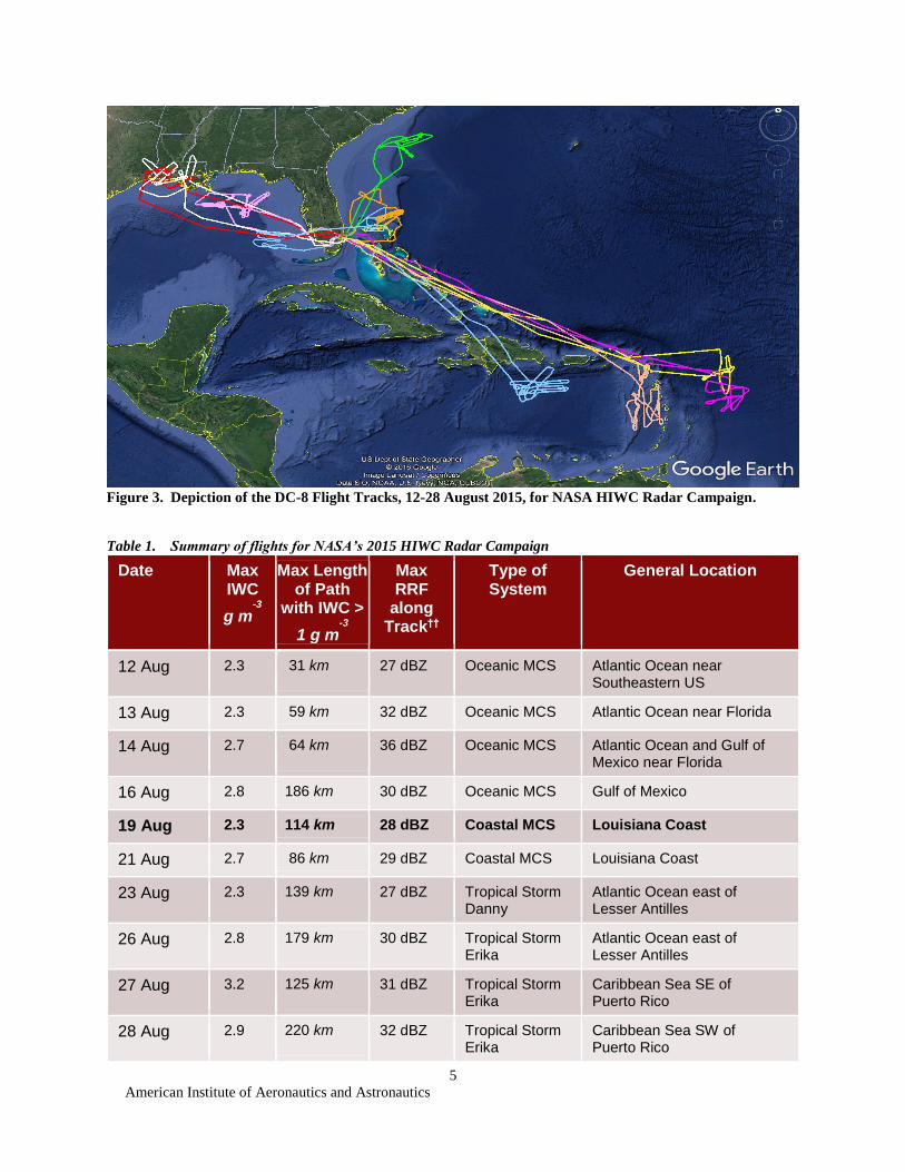
American Institute of Aeronautics and Astronautics
5
Figure 3 Depiction of the DC-8 Flight Tracks 12-28 August 2015 for NASA HIWC Radar Campaign
Table 1 Summary of flights for NASArsquos 2015 HIWC Radar Campaign
Date Max IWC
g m-3
Max Length of Path
with IWC gt
1 g m-3
Max RRF
along Trackdaggerdagger
Type of System
General Location
12 Aug 23 31 km 27 dBZ Oceanic MCS Atlantic Ocean near Southeastern US
13 Aug 23 59 km 32 dBZ Oceanic MCS Atlantic Ocean near Florida
14 Aug 27 64 km 36 dBZ Oceanic MCS Atlantic Ocean and Gulf of Mexico near Florida
16 Aug 28 186 km 30 dBZ Oceanic MCS Gulf of Mexico
19 Aug 23 114 km 28 dBZ Coastal MCS Louisiana Coast
21 Aug 27 86 km 29 dBZ Coastal MCS Louisiana Coast
23 Aug 23 139 km 27 dBZ Tropical Storm Danny
Atlantic Ocean east of Lesser Antilles
26 Aug 28 179 km 30 dBZ Tropical Storm Erika
Atlantic Ocean east of Lesser Antilles
27 Aug 32 125 km 31 dBZ Tropical Storm Erika
Caribbean Sea SE of Puerto Rico
28 Aug 29 220 km 32 dBZ Tropical Storm Erika
Caribbean Sea SW of Puerto Rico
American Institute of Aeronautics and Astronautics
6
As mentioned above no power-loss due to engine icing was noted during any of the flights however one TAT
anomaly and several Pitot tube anomalies did occur during prolonged encounters with high concentrations of ice
crystals
In section three we will summarize the observed characteristics of one of the flight days from the 2015 flight
campaign then in section five this event from this day will be examined via a numerical cloud model The numerical
cloud model the Terminal Area Simulation System (TASS) is summarized in section four In section six the same
numerical model and formulations also are applied to a benchmark case of a continental supercell hailstorm Findings
from both simulations are summarized in section seven The Appendix discusses an improved algorithm for
determining the size particle intercept for snow The relationship is derived from the August 2015 flight data and it
is applied in the numerical simulations for the coastal MCS as well as the continental supercell hailstorm
III 19 August 2015 Flight
Around 0730 UTC on 19 August a region of convection began to grow offshore of Galveston Bay Texas This
convection expanded to become a long-lasting coastal MCS that moved slowly east-northeastward along the Louisiana
coast (Figs 4 and 5) The MCS appeared to be sustained by bands of convection flowing into the system from the
Gulf and a large cloud canopy that capped the system covered much of Louisiana Developing cumulus towers
appeared to supply the southern end of these convective bands (Fig 6) Further upstream and underneath the cloud
canopy a region of steady rain fell over a wide area near the center and northern portion of the MCS
The most intense convection and the highestcoldest cloud tops were associated with the inflowing convective
bands located near the coast of Louisiana extending underneath the southern edge of the MCS cloud shield These
convective cells contained high radar reflectivity especially at low levels They also were very active with lightning
Movement of the convective cells were from the south-southwest toward the center of the MCS and new cells formed
at the southern edge to maintain the bands The lateral separation between the inflowing bans was roughly about 45
km This banded convection is evident from visible satellite but less so from infrared imagery due to partial
obscuration from the overhanging cloud canopy The MCS began to weaken after 1800 UTC as it moved through
southeastern Louisiana and into Mississippi
Figure 4 GOES Infrared Imagery for 1600 UTC 19 August 2015 Coldest cloud tops (purple ~205K) are along
the Louisiana Coast (Courtesy NASA Langley Satellite Group)
Eleven passes by the DC-8 were made through the MCS over a 4frac12-hour period (Fig 7) at elevations ranging from
29000 -37000 ft standard mean sea level (MSL) Ice crystals were encountered on these passes with sustained levels
American Institute of Aeronautics and Astronautics
7
at high concentrations measured on at least two of the passes The peak ice water content measured by IKP-2 was 23
g m-3 with the longest duration having 1 g m-3 or greater persisting over a 114 km path or during about 10 min of flight
Figure 5 Low-level radar reflectivity from NEXRAD Radar (left column) compared with visible satellite
imagery (right column) at 1600 UTC (top row) and 1645 UTC (bottom row) All four plots are of the same
spatial scale Banded convective lines are feeding into the MCS from the Gulf of Mexico
Figure 6 Lines of towering cumulus feeding into southern end of the Louisiana MCS and growing upward
through the overhanging cloud canopy Photographs from window of DC-8 courtesy of Stephanie DiVito (FAA)
American Institute of Aeronautics and Astronautics
8
Highest ice water concentrations seem to be located in the southern portion of the MCS where the convective
lines were feeding into the system The DC-8 encountered persistent regions of significant ice water concentration in
the two flight-legs along the Louisiana Coast but less so in other regions (Fig 7) Only weak concentrations were
measured in the northern regions and near the center of the cloud system where steady rain occurred
Although no engine irregularities were detected other events did happen Anomalies in airspeed due to icing of
both Pitot tube systems occurred during penetration of HIWC conditions Also during these ice crystal encounters
the DC-8 experienced 1) view of snow specks or ice particles hitting windows and being sucked into the engines 2)
IFR conditions 3) rime ice developing on both the Pitot tube and TAT probe outside the cockpit window 4) light
turbulence and 5) benign values of RRF appearing on the ship radar
This flight-day is of interest because of the storm systems structure which is unlike the MCS from the Darwin
Australia campaign that we have recently simulated10 In addition National Weather Service NEXRAD radar
(ground-based WSR-88D)16 data is available to supplement our analysis During many of the flights that were on other
days the DC-8 was not in range of ground-based radars
A scatter plot of the short-range (1micros pulse) airborne radar reflectivity factor vs measured ice water content for 19
August is shown in Fig 8 Values for IWC are measured by the IKP-2 and averaged over five seconds The criteria
for determining the RRF is that it must be detected within 1-km of the DC-8 Additionally it must be detected within
an altitude range of plusmn 150m (500 ft) of the flight path and laterally within the antenna azimuth angle of a beam width
(plusmn2 degrees) These criteria were put into place to best represent the RRF of the air that is actually encountered by the
aircraft Note that median values for RRF asymptote to near 20 dBZ when IWC increases to greater than 1 g m-3
Additionally there is a large range of scatter exists between RRF and IWC Although not shown plots from each of
the other days appear very similar having low values of RRF and a weak relationship to ice water content This would
suggest that RRF alone may be an unsuitable measurement parameter for detecting HIWC
An example from the display of the airborne research radar is shown in Fig 9 as the aircraft heads northeastward
across the Louisiana Coast This plot is sampled at a time when high ice water concentrations were being encountered
and the aircraft was passing over convective bands within the southern region of the MCS With level tilt the radar
displays mostly green (less than 30 dBZ) over a wide area Areas of higher reflectivity are evident with the downward
tilted scan and are associated with the convective bands crossing obliquely to the flight path Distinguishable radar
signatures for HIWC encounters do not seem to stand out
Figure 7 Flight path of DC-8 and measured ice water concentration from Ice Kinetic Probe for 19 August
2015
American Institute of Aeronautics and Astronautics
9
Figure 8 Peak short-range radar reflectivity factor (within 1-km of aircraft) vs ice water content measured by
IKP-2 for 19 August The median ice water concentration is represented by the red curve
Figure 9 One-hundred kilometer scan of radar reflectivity factor from the NASA Airborne Radar at 1634
UTC during HIWC encounter on 19 August for level tilt (left) and -4o tilt (right) Range rings every 5 km The
aircraft is at 885 km (29kft) MSL on an ENE baring just north of the Louisiana Coast
IV Numerical Model
A three-dimensional time-dependent numerical cloud model is used to investigate and shed further light on the
characteristic of this HIWC producing storm system Numerical simulations are performed with NASArsquos Terminal
Area Simulation System (TASS)171819 which has a history of being used to study microburst windshear 20212223
convection induced turbulence2425 aircraft wake vortices26272829 atmospheric boundary layer turbulence303132
tornadoes33 and severe convection34 Recently it has been applied to the study of HIWC such as a MCS convective
line observed during a HAIC-HIWC flight campaign at Darwin Australia10 The numerical model has prognostic
equations for velocity potential temperature pressure and water substances (water vapor cloud droplet water rain
water cloud ice crystal water snow and hailgraupel) TASS also has over 60 cloud microphysical submodels for
cloud and precipitation development The TASS formulation includes all three-phases of latent heat exchanges for
water and has a subgrid-turbulence closure formulation based on Vreman35 Boundary conditions can be periodic
American Institute of Aeronautics and Astronautics
10
open or closed and in combination The surface boundary is assumed flat and can represent either ocean or a flat
ground The impermeable surface boundary is nonslip with a parameterization for surface stress based on Monin-
Obukhov similarity theory36 Initiation packages are available for triggering cumulus convective systems turbulence
microbursts and aircraft wake vortices A summary of the salient characteristics of TASS are in Table 2 The TASS
model has over a 30-year history of supporting NASA programs37
Table 2 Salient Features in TASS
Ambient conditions initialized with atmospheric sounding
Arakawa C-grid staggered numerical mesh
Bulk parametrizations for cloud microphysics (over 60 sub-models)
Compressible time-split formulation
Efficient and accurate conservative numerical schemes with little or no numerical diffusion
Ground-stress based on Monin Obukhov Similarity Theory
History of application to aviation weather and safety problems
Initialization packages for convective storms microbursts turbulence planetary boundary layer and aircraft wake vortices
Large Eddy Simulation with subgrid scale turbulence closure
Liquid vapor and ice phase microphysics
Massively parallel interface scales efficiently with multiple processors as used on high-performance supercomputer clusters
Meteorological framework
Model simulations validated with field data and theoretical solutions
Monotone upstream-centered schemes for water substance
NonBousssinesq equation set
Nonreflective boundary conditions for open boundaries
Option of either open or periodic lateral boundaries
Option for either periodic or impermeable top and bottom boundaries
Prognostic equations for velocity pressure potential temperature dustinsects and water substance
Storm-tracking movable grid domain
Variable time step to ensure CFL criteria for numerical stability
Vreman subgrid turbulence closure model with modification for stratification and flow rotation
Water substance represented by water vapor liquid cloud water rain cloud ice snow and hailgraupel
Wet and dry growth for hail and snow
A Numerical Approximations
The TASS model equations are discretized using quadratic-conservative fourth-order finite-differences in space
for the calculation of momentum and pressure fields38 and the third-order upstream-biased Leonard scheme39 is used
to calculate the transport of potential temperature and water vapor A Monotone Upstream-centered Scheme for
Conservation Laws (MUSCL)-type scheme after van Leer4041 is used for the transport of water substance variables
Such a scheme is mostly free of negative water production from numerical error The Klemp-Wilhelmson time-
splitting scheme42 is used for computational efficiency in which the higher-frequency terms are integrated by
enforcing the CFL criteria to take into account sound wave propagation due to compressibility effects The remaining
terms are integrated using a larger time step that would be appropriate for anelastic and incompressible flows The
Adams-Bashforth scheme is assumed for time differencing of momentum and pressure for both large and small time
American Institute of Aeronautics and Astronautics
11
step approximations The TASS model is programmed in FORTRAN and operates efficiently on massively-parallel
computer architectures using Message Passing Interface (MPI) library calls
The numerics in TASS are very accurate highly efficient and nondissipative The integrity and accuracy of the
numerical and core dynamics is evaluated by performing a number of validation tests These include validation of
numerical simulations with special cases for analytical and existing high-order numerical solutions such as Beltrami
flow4344 compressible Taylor-Green Vortex454647 solutions and other test cases48 TASS has been found to achieve
high accuracy and efficient timing in these comparison tests Furthermore to ensure continued accuracy and fidelity
simulations from TASS are performed and evaluated against several baseline cases following any modification to
either the software or operating system These tests are designed to test most components and maintain efficiency
robustness and accuracy of the model
B Cloud Microphysics
TASS has over 60 bulk cloud microphysical submodels similar to those used by Lin et al49 and Rutledge and
Hobbs50 The autoconversion of cloud droplets into rain is based on drop growth studies by Berry and Reinhardt5152
and allows for differences in cloud droplet sizes usually found between continental and maritime locations17 Rain is
assumed to have an inverse-exponential drop distribution with an intercept that increases with rainwater
concentration53 in accordance with data measured by Sekhon and Srivastava54
The prediction of ice particles are divided into three different categories 1) ice crystal water mdash which represents
small hexagonal ice crystals 2) Snow mdash which represents larger precipitating ice particles and 3) hail (or graupel)
mdash which represents even larger more dense particles that are produced from freezing rain drops and riming snow
particles The ice crystal water is assumed to have a monodispersed particle size that is limited to diameters no greater
than about 200 microm These particles are represented by hexagonal plates have little fall velocity and grow primarily
by diffusion of vapor The snow category assumes spherical particles that have an inverse exponential size distribution
The size distribution intercept for snow Nos increases with decreasing temperature and snow water content The
relationship for Nos is developed from particle size distribution (PSD) data collected during the 2015 Florida flight
campaign and is described with more detail in the Appendix A category for hail and graupel particles also assume
an inverse exponential size distribution but with a smaller intercept and a larger particle density than for snow Wet
and dry growth for hail follows the formulation in Musil55 Several of the key parameters assumed for the particle
distributions are summarized in Table 3
Radar reflectivity factor is diagnosed in TASS based on the predicted water content and the assumed particle
distributions These relationships for RRF use the same particle distributions that are assumed in the microphysical
submodels The approach assumes Rayleigh scattering and is based on Smith et al56 For example the radar reflectivity
factor for rain is
119937119929 = int 119925(119915119929)infin
120782119915119929120788119941119915119929
The particle size distribution can be effectively represented by an inverse exponential distribution as
119925(119915119929) = 119925120782119929119942minus120640119915119929
where NOR is the intercept of the drop size distribution and λ is the slope The contribution of radar reflectivity factor
from rainwater can be determined with the relationship for NoR as assumed in deriving the microphysics used in TASS
(Table 3)
ZR [ mm6m3] = 94 x 103 Mr1468
where spherical drops are assumed and Mr is the rainwater content in g m-3 The radar reflectivity factor for ice particles consider the dielectric factors for ice and water and depend upon
whether the particle is undergoing either wet or dry growth For example the contribution to radar reflectivity factor
for ldquodryrdquo snow adjust for the melted diameters is
119937119930 =|119922119920|
120784
|119922119934|120784 120633119930120784
120633119960120784 int 119925(119915119930)
infin
120782119915119930120788119941119915119930 (1)
American Institute of Aeronautics and Astronautics
12
The values assumed for the dielectric factors are for wavelengths employed in weather Radars57 The contribution to
RRF from hailgraupel ice crystals and cloud droplets are computed similarly For ldquowetrdquo hail the contribution is
adjusted for Mie scattering as in Smith et al56
Table 3 Key relationships and assumptions in TASS Microphysics
Category Size Distribution and
Intercept (m-4)
Particle Density ( )
Comment
Liquid Cloud Water
Monodispersed
1000 kg m-3
NCD number of droplets per volume is an input
Rain Inverse exponential
NOR = 225 x 107 M
R
0375
1000 kg m-3
Intercept increases with rainwater content
MR (g m
-3)
Cloud Ice Crystal Water
Monodispersed
Particle mass (kg) =
01758 Dic
22
Hexagonal plates Diameter mostly lt 200 microm
Snow Inverse exponential
NOS = 10(744 ndash 00217 Tc+ X)
where
X = Ms [1053-M
s (015-
0004Ms )]
for 4oC gt Tc gt -55
oC
100 kg m-3
if
Tc lt -12 oC
Ramping to 150 kg m-3
at
Tc gt 0 oC
Intercept increases with decreasing temperature
and increasing snow
concentration Ms (g m
-3)
HailGraupel Inverse exponential Intercept is an input
parameter
Either 450 kg m-3
if graupel or
900 kg m-3
if hail
Intercept decreases with temperature when Tcgt 0oC
V Numerical Simulation of 19 August Case
In this section the numerical simulation from the 19 August case is presented to help better understand the
characteristics of this system Comparisons with measured data are presented to substantiate the credibility of the
numerical simulation
A Configuration
In modeling the HIWC conditions associated with this convective system an approach similar to that used in the
Darwin HIWC simulation10 is used The domain of the model simulation is defined to represent a section of the MCS
rather than the full volume surrounding the weather system Specifically the modelrsquos computational domain is
specified about one of the inflowing lines of convection (Fig 10) Periodic lateral boundary conditions are assumed
on the domain boundaries parallel to the convective line and open lateral boundary conditions assumed on the ends
This configuration allows the simulated line to interact as if identical parallel lines exist on either side This includes
the interaction of the canopy outflow with the adjacent convective lines via the periodic boundaries The domain also
is rotated 21o to align the model y-axis with the direction of the low-level shear vector This results in the model
domain being oriented along the convective line since observed convection often orients itself in a line along the low-
level shear vector
The domain size and resolution (Table 4) is chosen to simulate the physics adequately and to resolve the essential
three-dimensional scales of motion The domain width of 45 km is based on the typical distance separating the
inflowing convective lines The grid size is chosen to concentrate the model grid points into a 45km x 150km area
American Institute of Aeronautics and Astronautics
13
The assumed grid size is the same in all three
directions (150m) and is small enough to allow the
resolution of important thermally-driven scales of
motion
The atmospheric sounding used as input is
extrapolated from an operational weather forecast
model at a location just upstream from the system
This sounding (Fig 11) possess strong convective
instability and deep levels of moisture This sounding
also indicates a tropopause at 14km MSL with a
temperature of about -62oC or 211K Convective
indices58 computed from the sounding indicate strong
convective instability with a lifted index of about -6oC
and CAPE = 3400 J kg-1 The melting level is at
4900m MSL
The initial state of the numerical simulation is
horizontally homogeneous and varies vertically
according to the input sounding shown in Fig 11
Convection is initiated by an artificial thermal
impulse A cool pool of air that resides near the
surface over much of Louisiana and underneath the
MCS is ignored for the initial and boundary
conditions The boundary conditions for the ground
are representative of a smooth ocean surface with
constant temperature Other input parameters for the
simulation are representative of a tropical oceanic
environment (Table 5) The simulation is integrated
over a 4-hour period with convection occurring
through the full period In our simulations time (t) is in reference to time of initiation and values for the x and y
coordinates are in reference to the initial triggering impulse
B Results
The numerical simulation generates a long-lasting system with a convective line oriented in the direction of the
low-level shear vector of the environmental winds The cyclic (ie periodic) boundary conditions on the left and right
sides of the domain account for the effect of multiple lines including the interaction between the lines The type of
convection is multicellular11 with overshooting tops penetrating through the tropopause by about 600 m The system
produces persistent HIWC conditions at storm upper levels within an expanding cirrus shield fed from the multi-
Figure 11 Skew-T diagram representing initial
environmental profiles for 19 August 2015 case
Modified from sounding extracted from an operational
weather model forecast at 1400 UTC at location
upstream from the MCS (29N 912W)
Figure 10 Model Domain size relative to MCS
Table 4 Domain Size and Resolution
Domain Parameter Physical Dimension
Lateral dimensions (X Y) 45 km x 150 km
Vertical dimension (Z) 186 km
Lateral grid spacing 150 m
Vertical grid spacing 150 m
Computational grid ~39 x 10
6
grid points
Table 5 Initial Parameters
Cloud base height 625 m (942 mb)
Cloud droplet number density Ncd 75 droplets cm-3
HailGraupel particle size distribution intercept Noh
4 x 10⁵ m-4
American Institute of Aeronautics and Astronautics
14
cellular convection A comparison of the low-level radar reflectivity factor from the model simulation with the
observed NEXRAD reflectivity is shown in Fig 12
Figure 12 Comparison of low-level RRF between NEXRAD (left) and TASS (right) Observed NEXRAD
for Louisiana coast at 1645 UTC Simulated RRF at 4km altitude and 3hr 45min Outline of TASS domain
shown (90 km x 150 km)
Updrafts within the convective line generate precipitation and carry snow particles and ice crystals to the upper-
regions of the troposphere At upper levels the expanding outflow coalesces with the upper-level anvil outflow from
adjacent lines to form a large overhanging canopy (Fig 13) The general comparison between observations and
numerical simulation are summarized in
Table 6
Horizontal cross-sections at two
altitudes for RRF and IWC are shown in
Figs 14 and 15 The chosen altitudes
represent the two flight altitudes for the
DC-8 during each of two passes when
persistent IWC was measured The timing
of the slices are at a model time of
3hr45min (from the start of initialization)
and represent a time when the simulated
system has reached a mature state Profiles
are extracted along the dashed line shown
in the figures and are compared to that
measured by the DC-8 (Fig 16)
In Fig 14 the numerically simulated
ice water concentration (ice crystal snow
and graupel water combined) as well as the
RRF are shown at flight level 29 kft (8850 m) Peak ice water concentrations exceeding 3 g m-3 can be found within
small areas associated with the convective updraft turrets Larger areas with a width of about 40km exceeded 1 g m-3
Radar reflectivity factor values are generally less than 30dBZ and would appear green on the weather radar display of
most aircraft Locally higher values of RRF were found within the strong updraft cores that carry graupel and other
ice particles The RRF in Fig 14 does show large areas of low RRF but not as uniform as from the flight radar (cf
Fig 9) A more appropriate comparison would be between the RRF observed by the DC-8 with a simulation of its X-
band radar using the TASS fields as input
Figure 13 Simulated three-dimensional cloud surface viewed
from above and from south-southwest
American Institute of Aeronautics and Astronautics
15
Table 6 Comparison of general features between observed and numerically simulated for 19 August 2015 case
Feature Observed Simulated with TASS
Orientation of convective lines SSW-NNE with 45 km separation between lines
SSW-NNE with 45 km separation between lines
Cloud top elevation ~14-15 km 146 km
Coldest cloud top temperature ~200 K 203 K
Cell movement from 210o at 10 ms 221o at 11 ms
Direction of anvil canopy expansion from Southwest Southwest
Convective line movement from 290o at 6 ms 291o at 45 ms
System lifetime gt 10 hrs gt 4 hrs
Width of area with RRFgt20 dBZ at cruise altitudes
gt 50 km 40 km
At a slightly higher altitude (Fig 15) regions with HIWC cover smaller areas and have lower values of RRF This
is consistent with the measurements from the DC-8 which encountered shorter durations of IWC greater than 1
g m-3 and detected lower values of RRF after changing to a 5kft higher altitude on a subsequent pass through the
active regions near the Louisiana coast
Figure 16 shows a comparison of measured and model-extracted profiles for RRF and IWC The DC-8 flight
profiles relative to the MCS are shown in Fig 17 The TASS profiles are extrapolated at the two different altitudes
and headings flown by the DC-8 and are compared with values measured by the DC-8 At the lower elevation both
the TASS and DC-8 profiles indicate a nearly steady RRF of about 20-25 dBZ and IWC mostly between 1- 25 g m-3
At the higher elevations both TASS and DC-8 show consistent magnitudes of variation with the RRF varying between
0 to 20 dBZ and the IWC mostly remaining below 05 g m-3 Both profiles at the higher elevation do show a small
region where IWC approached 2 g m-3 Although peak values and duration of encounters seemed similar in magnitude
the variability of RRF and IWC appears greater in the modeled profiles
In Fig 18 vertical cross-sections of the simulated RRF and IWC fields are taken along the assumed flight path in
Fig 14 Note that large regions of IWC greater than 15 g m-3 (orange) extend over a large region along and below the
lower-altitude flight path Peak values occur between altitude ranges of 75-95 km AGL and drop off significantly
above 10 km AGL The corresponding RRF shows larger values below the melting level (around 5 km AGL) and very
weak values above 10 km MSL Also note that regions with significant IWC can extend above regions with low or no
detectable RRF near the ground
In summary a persistent coastal MCS system with HIWC is numerically simulated and its results compared with
data from the 2015 Florida Radar flight campaign The system is sustained by bands of convection inflowing from the
Gulf of Mexico and is capped by a large canopy cloud consisting of mostly ice crystals The simulation showed that
the coalescence of the expanding anvils from the convective cells resulted in a cloud canopy that may obscure the
banded structure and other low-level features from detection with satellite The model simulated cloud top elevations
and movement of cells appear similar to observations Largest concentrations of ice water were found in the simulation
between 75 and 95 km (25kft-31kft) MSL where environmental temperatures were between -19oC to -33oC The
range of elevations with the largest RRF were between the surface and 6km (20 kft) MSL The TASS-extracted profiles
compare reasonably with the measurements from DC-8 although some differences in variability were noted
American Institute of Aeronautics and Astronautics
16
Figure 14 Simulated RRF (left) and IWC (right) from TASS simulation at an altitude of 8850m (flight level
29kft) and 3hr and 45 min The TASS IWC field is the sum of all ice water (ice crystal water + snow + graupel)
Figure 15 Same as Fig 14 but at 10335m (flight level 34 kft)
American Institute of Aeronautics and Astronautics
17
Figure 16 Comparison of RRF and IWC extracted along flight profiles shown in Figs 14 and 15 (dashed
lines) with those measured by the DC-8 (solid lines) Top row at an altitude of 8850m bottom row at 10350m
Figure 17 Two of the DC-8 legs with longest duration of IWC
Track of DC-8 superimposed on 1645 UTC GOES-13 Infrared
satellite imagery (Courtesy NASA Langley Satellite Group)
American Institute of Aeronautics and Astronautics
18
Figure 18 Vertical cross sections of RRF (top) and IWC (bottom) extrapolated from the numerical
simulation along the flight profile shown in Fig 14 Vertical position of both flight paths shown by dashed line
Altitudes are AGL
The numerical simulation does not capture the region of stratified precipitation that lies downstream from the
inflowing convective lines However the DC-8 flights did not encounter regions of HIWC when they overflew this
region It appears likely that the rain in this area was produced by moisture from the dissipation of the convective cells
and the overrunning of the cool surface dome by the moist southerly air currents A next-generation simulation would
need to include the horizontal variation of temperature and wind into the simulation in order to capture these effects
VI Numerical Simulation of Continental Supercell Hailstorm
In this section the numerical simulation of a continental supercell hailstorm is presented The purpose of this
simulation is to validate the robustness of the microphysics used in TASS and better understand differences in HIWC
production between continental supercell storms and subtropical MCS convection Validation parameters include 1)
production of large hail 2) size of hail swath 3) radar bounded weak echo region 4) supercell features 5) storm
motion 6) size and intensity of quasi-steady updraft 7) size and maximum value of radar echo and 8) duration In
this simulation we will verify the validity of the simulation by comparing our solutions with observed data In
addition this case will be analyzed for its potential in producing HIWC and compared with the previous case of
summertime coastal convection
This case has been simulated in the past with one of the first versions of TASS using a relatively coarse mesh
Even at this earlier stage of TASS development the simulation was able to capture many of the stormrsquos observed
features5934
A Description of Observed Case
On 2 August 1981 a very large and severe hailstorm moved across Southeastern Montana The storm was observed
during its mature phase with ground-based Doppler radars and with research aircraft as it moved through a network
of field instruments during the Cooperative Convective Precipitation Experiment60 (CCOPE) The storm quickly
developed many classical features of a supercell hailstorm It veered to the right of the environmental winds and
persisted for over 5 hours while leaving a wide swath of hail The storm was reported to have an intense quasi-steady
updraft with cyclonic rotation a low-level radar hook echo signature a mid-level bounded weak echo region (BWER)
signature (same as radar echo vault) damaging winds a broad swath of 1-3 cm diameter hail with some sizes as large
American Institute of Aeronautics and Astronautics
19
as 10 cm a mesolow or mesocyclone with a peak pressure drop of at least 6mb and a peak RRF between 65-75
dBZ61626364 The primary updraft of the storm was reported to be over 14 km wide and was located within the BWER
A research aircraft flew within the updraft at an altitude between 6 km and 75 km MSL they found nearly adiabatic
conditions with updraft speeds greater than 50 m s-1 liquid water droplet concentrations of up to 6 g m-3 and the
absence of precipitation-sized particles65 The lack of larger particles explained the very low magnitudes of RRF within
the BWER Hail was penetrated by the research aircraft on the western edges of the updraft in association with the
high reflectivity regions Weisman et al66 reported that the storm produced at least one funnel cloud and that some
damage reports were ldquosuggestiverdquo of tornadic activity Surface wind speeds were estimated between 50 to 100 mph
(20 to 45 m s-1)63
A special rawinsonde sounding was launched near the storm (Fig 19) and indicated an environment very favorable
for intense convection Convective indices
calculated from the sounding exhibited a CAPE of
almost 3500 J kg-1 and a lifted Index of -10oC
The sounding also indicated a tropopause height
of 109 km MSL (~99 km AGL) with a
temperature of -475oC and an equilibrium level
at 198 mb (123 km MSL) with a temperature of -
517oC According to the both the sounding and
aircraft observations the cloud base temperature
and height were about 136oC and 26 km MSL
respectively63 The ground was slightly less than
1km above sea level and varied somewhat with
location The wind profile for the sounding
exhibited a strong magnitude of helicity6768 and
vertical shearing of the environmental wind High
values of both helicity and CAPE are indicative of
supercell and tornadic storm environments The
presence of dry environmental air at storm mid-
levels likely inhibited any strong tornado
formation (eg Proctor et al33)
B Configuration
In numerical modeling of this system we apply the
same version of the TASS model as in the Coastal-MCS
case Differences are only due to grid and domain
configuration boundary conditions input sounding and
several input parameters that define the continental
aspects of the cloud droplets and the hail size
distribution All are discussed below
The domain is size is defined to be 150 km x 150 km
in the horizontal and 20 km in the vertical (Table 7) An
evenly spaced grid size of 200 m is assumed Open
lateral boundaries conditions are applied at all lateral
boundaries The ground surface is assumed flat and no
terrain features are included The domain uses the
TASS modelrsquos internal tracking algorithms17 in
order to move the grid with the lateral translation of
the storm
The initial state profiles for temperature
pressure wind and humidity are horizontally
uniform but vary vertically according to the input
sounding shown in Fig 19 Values representative of
contental Great-Plains systems are assumed to for
the cloud droplet concentration and for the hail size
distribution intercept parameter (Table 8)
Figure 19 Skew-T diagram representing environment for
2 August 1981 Special sounding observed near Knowlton
MT at 2356 UTC Environmental wind hodograph
inserted at bottom left
Table 7 Domain Size and Resolution
Domain Parameter Physical Dimension
Lateral dimensions (X Y) 150 km x 150 km
Vertical dimension (Z) 20 km
Lateral grid spacing 200 m
Vertical grid spacing 200 m
Computational grid ~56 x 10
6
grid points
Table 8 Initial Parameters
Cloud base height (AGL) 1700 m (740 mb)
Cloud droplet number density Ncd 800 droplets cm-3
HailGraupel particle size distribution intercept Noh
2 x 10⁴ m-4
American Institute of Aeronautics and Astronautics
20
The major diffences between the initial conditions of this case and the coastal MCS case are that this case
represents a more continental environment with stronger vertical wind shear less moisture but greater instability
C Comparison of Simulation with Observations
The numerical simulation is initiated at time zero by introducing a thermal impulse and integrating over 4 hours
of time The simulation produces a supercell hailstorm and captures many of the features observed in the real storm
These include large hail wide hail swath funnel cloud with damaging surface wind 15 km wide quasi-steady updraft
surrounded at storm-mid-level by a radar echo vault or BWER a radar hook echo signature right-rear quadrant gust
front massive overshooting tops and a large spreading anvil As can be see in Table 9 scales and intenisties match
very well between the observed and simulated event The simulated updraft velocity at 65 km MSL of 55 m s-1 matches
the peak value measured by a research aircraft that penetrated the storm at the same level As found from the aircraft
measurments the updraft core was nearly adiabatic with little or no precipitation The model simulation as in the
observational studies found most of the hail to be on the western and nortwestern edges of the primary storm updraft
Table 9 Comparison of observations with TASS for 2 August 1981 Supercell Hailstorm
Features Observed TASS Simulated Anvil Extent Downstream from Updraft
(based on Radar Echo) gt200 km gt150 km
Anvil Extent Upstream from Updraft gt20 km gt60 km
BWER Diameter ~75 km ~8 km
BWER Vertical Extent 10 75 km MSL 12-14 km MSL
Gust Front Location SW Flank SW Flank
Peak Gust Front Wind Speed gt20 ms 25 ms
Typical Hail Diameter at Surface 1-3 cm peak median diameter 2 cm
Hail Shaft Location Relative to Center of BWER 3-4 km West 4-6 km WNW
Width of Hail Swath 20-30 km 225 km
Supercell Lifetime gt 5 hrs gt 4 hrs
Persistent Low-Level Radar Hook Echo yes Yes
Maximum Liquid Cloud Water Content 65 g m-3 55 g m-3
Surface Pressure Drop 6 mb Mesocyclone 4 mb tornado 21 mb
Peak Rainfall Accumulation 30-35 mm 25 mm
Peak Radar Reflectivity Factor 75 dBZ 726 dBZ
Storm Movement (development stage) 260 at 10 ms 250 at 12 ms
Storm Movement (supercell stage) 282 at 18 ms 280 at 16 ms
Storm Top Overshoot above EL 3-4 km 5 km
Updraft Diameter 14-17 km 15 km
Max Updraft Velocity at 65 km MSL 53 ms 55 ms
Diameter of 20 dBZ Echo at 12 km MSL 45 km 45 km
Peak Surface-Level Gusts East of Updraft gt25 ms 30 ms
Radar Echo Top 16 km MSL 18 km MSL
Tornadoes Funnel cloud sighted Yes western side of mesocyclone
Peak Surface Wind Damage F1- wind damage (estimated 33-50 ms)
56 ms
Maximum Altitude of 10 dbZ Contour in BWER 6-8 km MSL 65 km MSL
American Institute of Aeronautics and Astronautics
21
Supercell environments often produce tornadoes or familes of tornadoes and a funnel cloud with surface wind
damage was reported with this system The funnel cloud that was produced in the numerical simulation was
intermittent and dissiapted when it moved into the cooler dryer air underneath the hail and rain shafts Tornado
formation in this simulation showed similar characteristics to those studied in an earlier paper where the presence of
dry mid-level air acts to weaken or suppress tornado formaition in supercell environments33
The time evolution of the area with RRF greater than 55 dBZ at an elevation of 5 km MSL (blue) and the peak
RRF anywhere in the storm (red) is shown in Fig 20 The peak RRF from the simulation matches the observations
very well For the area with RRF greater than 55 dBZ both observation and TASS show a ramp up in the first two
hours of the stormrsquos lifetime but the
simulation shows this area to be smaller
than detected by ground-based radar
A comparison of the supercell structure
from TASS with measurements from
ground-based radar are shown in Figs 21
and 22 Two horizontal levels of RRF are
shown one at 10 km MSL and the other at 4
km MSL The TASS simulation reproduces
many of the observed features and supercell
signatures including the BWER (ie radar
echo Vault (V)) the radar hook echo and
the radar echo streamer The scale of the
area covered by each intensity of RRF are
similar between TASS and observed as
well One contrast however is that the high-
reflectivity area within the hook echo region
appears larger in the observation than in the
simulation The area of highest reflectivity
which is west and northwest of the BWER
is associated with large hail in both
observation and simulation
In Fig 23 a vertical cross-section along
x-z coordinates is taken through the middle
of the BWER Again both the simulation and observation show similar features similar intensities and similar spatial
scales The BWER or radar Vault is clearly present in the simulation and extends deep into the storm The BWER
is located within the intense storm updraft and is produced by a lack of significant precipitation-sized particles
D HIWC Characteristics in Simulated Storm
The Montana supercell with its quasi-steady large diameter and intense updraft generates large volumes of ice
crystals that are transported into the upper regions of the troposphere Increasing wind speeds with height which is a
characteristic of supercell environments quickly transports many of the ice particles downstream within a large
expanding anvil cloud Hail and larger ice particles are also carried up to high altitudes by the strong updrafts but fall
out relatively close-by due to their significant fall velocities Therefore large values of RRF can be found at storm
upper-levels within proximity to the supercell updraft The RRF drops-off with distance from the updraft as the larger
particles fall out and the remaining smaller particles are carried downstream
A graphical representation of the cloud and precipitation fields from TASS is show in Fig 24 Overshooting tops
which are above the predominant supercell updraft can penetrate several kilometers into the stratosphere A large
anvil cloud spreads mostly downstream from the overshooting tops due to the strong westerly winds beneath the
tropopause (cf Fig 9) This anvil cloud covers many square kilometers and forms a large overhang of cloud material
downstream from the storm updraft Due to the intensity of the updraft some the anvil material is transported counter
to upper-level winds and produces a forward overhang upstream from the storm updraft
The coldest cloud tops (Fig 25) are associated with the overshooting tops above the intense storm updraft Cloud
tops at temperaturesheights near the equilibrium level expand over a large area downstream from the overshooting
tops Obviously in Fig25 the anvil expands northeastward beyond the boundaries of the model domain
Figure 20 Time evolution of the maximum RRF anywhere
in the storm (red) and the cross-sectional area of reflectivity
exceeding 55 dBZ at 5km MSL (blue) Observed values from
Miller et al63(solid) compared with TASS (dashed)
American Institute of Aeronautics and Astronautics
22
Figure 22 Same as Fig 21 but RRF at an elevation of 4 km MSL Left adapted
from Millerrsquos analysis of ground based Doppler radar right from TASS at
t=3hr07min
RRF (dBZ)
Figure 21 Horizontal cross-section of Radar reflectivity factor at an altitude of
10 km MSL Left adapted from Millerrsquos analysis of ground based Doppler radar62
right from TASS at t=3hr07min Both plots windowed to 50km x 50km area with
major tick every 10 km The Radar echo Vault or BWER identified with V
Figure 23 Same as Fig 21 but RRF along vertical west-east cross-section through
BWER Left adapted from Millerrsquos analysis of ground based Doppler radar right from
TASS at t=3hr07min Altitude in km AGL with major ticks every 1km along abscissa
American Institute of Aeronautics and Astronautics
23
Very similar features for the simulated Montana supercell storm can be seen in the observed visible satellite
imagery of the actual system (Fig 26) The overshooting tops are positioned near the southern end and the anvil
expands toward the north-northeast The horizontal dimension of the observed cloud anvil compared with the cloud
top depicted in Fig 25 are nearly identical
Figure 27 shows the simulated IWC and RRF along a horizontal cross-section taken at 10km MSL (9km AGL)
The size and shape of the system represented in the cross-section is consistent with the satellite imagery in Fig 26 In
Fig 27 most of the RRF greater than 20 dBZ is confined to area within a 50 km diameter centered about the primary
updraft and BWER Values of RRF between 15-20 dBZ cover large areas downstream for the overshooting tops
Figure 27 also shows vast areas with IWC greater than 1 g m-3 In fact areas with 1 g m-3 or greater can be found at
distances of up to 50 to 100 km away from the regions with the greatest storm RRF Our simulation seems to imply
that by avoiding the high reflectivity areas by 20 nautical miles (37 km) may not be sufficient for avoiding prolonged
HIWC exposures
Figure 24 Simulated cloud and precipitation surfaces within the full TASS domain Viewed from south
Figure 25 Cloud top temperatures from TASS at 3hr75 min (left) and 3hr45min (right) simulation
time Coldest temperatures associated with overshooting tops in southwestern quadrant of figure
American Institute of Aeronautics and Astronautics
24
To further explore the structure of the simulated storm
vertical cross-sections are extracted alone lines A-B and C-D
that that appear in Fig27 These cross sections are shown in
Figs 28 and 29 They also help illustrate where HIWC
conditions may be found relative to the storm
The cross-sections through A-B (Fig 28) are taken
northeastward through the storm updraft It shows strong
reflectivity surrounding the BWER and extending to the upper
levels of the storm High levels of IWC largely composed of
hail are brought to the ground on the southwestern side of the
storm updraft and at upper-levels surrounding the updraft
Aircraft routinely avoid these areas due to their high values of
RRF More of a factor to air traffic is that significant levels of
IWC that can be found over large areas within the cloud
canopy at great distances downstream from the stormrsquos high
reflectivity regions Furthermore the RRF within the canopy
are very low and could be undetectable with many airborne
weather radars
In Fig 29 a cross section is taken orthogonal to the
direction of the shearing anvil It is taken northwestward
between C and D along the edge of the areas with significant
IWC (Fig 27) This cross-section resides at least 70 km or
more from areas with high RRF Along this cross section IWC
greater 1 g m-3 can be seen to extend for over a 100 km length
The layer has a thickness that is several kilometers thick This
layer also consist of very weak RRF (lt 20 dBZ) and
underneath has no detectable radar reflectivity or precipitation
Both cross-sections show that a layer with HIWC can extend over large distances and with very weak RRF
Beneath this layer containing HIWC precipitation was rarely apparent and radar reflectivity not detectable One visual
queue sometimes recommended to pilots for helping to identify potential HIWC conditions is the presence of strong
to moderate RRF from rain beneath regions of HIWC This queue would not apply to a supercell storm such as this
This case of a continental supercell also demonstrates that HIWC risks may not be confined to just oceanic and
coastal MCS since regions of significant IWC may extend for large distances with little RRF
VII Discussion and Conclusion
Flight data and results from numerical simulations are analyzed to better characterize the HIWC threat for aircraft
and to improve our understanding of the relationship between HIWC radar and satellite signatures Flight
measurements with airborne radar and microphysical probes suggest that RRF alone may not be adequate for the
detection of HIWC conditions This fact also is reinforced from the numerical model simulations
The numerical simulations confirm that HIWC can be produced in contrasting environments In warm moist
coastal and oceanic environments large volumes of ice crystals can be pumped into the upper-troposphere by
regenerating convective plumes associated with a long-lasting system Cloud material carried in the upper-level
outflow from these plumes coalesces to form a large overhanging canopy and contain significant concentrations of
ice crystals Perhaps due to the weaker wind shear of these environments and the duration of the systems large
concentrations may accumulate over time
Our simulation of a large continental supercell shows it to have a large persistent and nearly adiabatic updraft
that also can pump large volumes of ice crystals in to the upper troposphere Vertical windshear with strong winds
aloft (which are an ingredient in producing supercells) can act to transport ice crystals over large areas We speculate
that the increase ventilation due to environmental wind shear may dilute the peak concentrations of IWC in supercells
Figure 26 Observed visible satellite imagery
from GOES-7 Northeastern Montana 2315
UTC 2 August 1981
American Institute of Aeronautics and Astronautics
25
Figure 27 Ice water content (left) and RRF (right) from TASS at an elevation of 10km MSL and 3hr45
min) simulation time Ice water content (g m-3) is sum of ice crystal snow and hail water content Units
for RRF are (dBZ)
Figure 28 Vertical cross section along A-B in Fig 27 Top is ice water content (g m-3) and bottom is RRF
(dBZ) Altitudes are above ground level
American Institute of Aeronautics and Astronautics
26
In our study the microphysics for snow is improved by using analyzed PSD data measured during the flight
campaign A new relationship is developed that relates the exponential size-distribution intercept for ice particles with
their water content In the past the value for the intercept has been assumed constant or a function of temperature
only The new relationship is a function of snow or ice water content as well as temperature and was used to improve
the microphysical submodels in TASS
The TASS model was then applied to contrasting types of convection and compared to available observations
This comparison seemed very good and demonstrated the model could be applied robustly to convection in different
types of environments Excellent results were achieved using only simple bulk parametrizations for microphysics
suggesting that models that are more complex may not be needed depending upon application The profiles of ice
water content and RRF extracted from the simulation compared reasonably well with the measurements by the DC-8
during penetrations of the coastal MCS although some differences in variability were noted The TASS model was
also used to simulate a specific supercell hailstorm with excellent comparison to measurements in terms structure
features scales and magnitudes
The numerical studies for both cases found that regions of significant IWC could extend above regions with little
or no RRF This would imply that moderate to high radar reflectivity might not always be underneath HIWC events
Yet to be investigated is the potential for HIWC detection using a combination of sensors and sources for
information (ie satellite and other weather data) Also unexplored is the ability to detect HIWC with advanced
airborne radar tools
Appendix Ice Crystal Size Distributions
Relationships between the ice crystal size distributions temperature and ice water content are needed for the
parameterization of microphysical submodels used in TASS These relationships could be useful in other applications
such as the understanding the radar reflectivity factor (RRF) due to ice crystals Dr Alexei Korolev processed the
particle size distribution (PSD) data69 from data collected at one-Hertz intervals during the DC-8 flights from a 2D-S
probe and a particle-imaging probe (PIP) The measured data was discretized into appropriate size bins and normalized
by the width of the corresponding bin This allowed for the direct comparison of the PSD data with different size
resolutions and common theoretical drop-size distributions (eg Marshall-Palmer70) The size resolution for the 2D-S
probe was10 μm and 100 μm for the PIP The range of particle measurements extends from 15 μm to 12845 mm The
Figure 29 Same as in Fig 28 but for position C-D in Fig 27
American Institute of Aeronautics and Astronautics
27
size of irregularly shaped ice particles as estimated from particle images may be defined in several different ways
The composite PSD data used the length of the particle parallel to the photodiode array commonly called Ly
An intercept (N0) and slope (λ) parameter were found from the data by using a least-squares method to fit an
exponential distribution through the measured PSD This was repeated for all times in a flight Relationships can then
be established for N0S vs ice water content (IWC) and atmospheric temperature
Our numerical modeling effort previously employed a relationship for Nos that is a function of temperature
only1017 Recall that our snow category represents the larger ice particles (excluding graupel and hail) and assumes
an inverse exponential size distribution whereas our cloud ice category only represents the smaller ice particles with
diameters less than about 200 um Using combined data measured from each day of the NASA deployment (Table 1)
and binning according to temperature a new relationship was determined for Nos that is a function of both temperature
and snow water content Ms
Log10 (Nos) = 744 ndash 00217 Tc +10526 Ms ndash 015 Ms2 +0004 Ms3 (A-1)
for Tcgt -55OC and Ms lt 4 g m-3
where Nos has units of m-4 Ms has units of g m-3 and Tc is temperature of the environment in centigrade The
relationship was fitted from the flight data as shown in Fig A1 and produces a larger intercept value for either colder
temperatures or increasing snow water content A higher intercept value translates into a distribution with overall
smaller particles lower radar reflectivity factor and slightly slower fall velocity Other parameterized microphysical
processes are affected by the assumption for Nos these include sublimation or deposition of snow particles and other
growth processes
Note that when Ms 0 the above relationship asymptotes to a relationship suggested by Woods et al71 who
derived their relationship from analyzing ice particles in wintertime precipitation occurring in the Pacific Northwest
Based on all ice particles they found the following relationship for No
Log10 (No ) = 753 ndash 00207 Tc (A-2)
Since their measured ice water contents ranged between 003 and 030 g m-3 it would have been difficult for them to
detect any dependency of No on ice water content
As a further check to the validity Eq (A-1) we compare the observed short-range RRF with the value estimated
from the measured IWC using the assumption of an inverse exponential size distribution with Eq (1) as
ZS [mm6m3] = 390 x 108 Ms175 Nos
-075 (A-3)
where the above assumes melted spherical particles and accounts for the differences in radar dielectric constants for
ice and water
The comparisons are shown in Fig A1 and illustrates the lack of correlation of radar reflectivity with snow water
concentration for values of snow water greater than about 1 g m-3
American Institute of Aeronautics and Astronautics
28
Figure A1 Ice particle distribution intercept NoS
vs ice water content for three temperature ranges
Data points derived from PSD distributions
measured during all 2015 DC-8 Flight Campaign
flights (ie Table 1) Blue curve represents medium
value Red curve is fit using Eq (A-1)
Figure A2 Radar reflectivity factor vs ice
water content for three temperature ranges
Data points of close-range RRF measured during
all 2015 DC-8 Flight Campaign flights (ie Table
1) Blue curve represents medium value Red
curve using Eqs (A-3) and (A-1)
American Institute of Aeronautics and Astronautics
29
Acknowledgments
This research is sponsored by the Advanced Air Transport Technology Project of NASArsquos Advanced Air Vehicles
Program The authors would like to acknowledge the contributing organizations that enabled the Florida HIWC Radar
Flight Campaign the FAA Aviation Research Division and Aviation Weather Division the NASA Aviation Safety
Program the Boeing Company Met Analytics Science Engineering Associates Environment Canada the National
Center for Atmospheric Research Honeywell and Rockwell Collins The authors also would like to thank Tom
Ratvasky (NASA Glenn Research Center) and Walter Strapp (Met Analytics) for their programmatic technical and
operational support and the NASA Langley Satellite Group for providing satellite images In addition thanks to
Alexei Korolev (Environment and Climate Change Canada) for processing the PSD data from raw data collected
during the flight test The numerical simulations were conducted using the Pleiades high-performance supercomputer
cluster of the NASA Advanced Supercomputing Division
References
1Mason JG Strapp JW and Chow P ldquoThe Ice Particle Threat to Engines in Flightrdquo AIAA 2006-206 doi10251462006-
206 2Mason JG and Grzych M ldquoThe Challenges Identifying Weather Associated with Jet Engine Ice Crystal Icingrdquo SAE
International 2011-38-0094 doi1042712011-38-0094 3Bravin M Strapp JW and Mason J ldquoAn Investigation into Location and Convective Lifecycle Trends in an Ice Crystal
Icing Engine Event Databaserdquo SAE International 2015-01-2130 doi1042712015-01-2130 4Addy HE Jr and Veres JP ldquoAn Overview of NASA Engine Ice-Crystal Icingrdquo SAE International 2011-38-0017
doi1042712011-38-0017 5Grandin A Merle J-M Weber M Strapp JW Protat A and King P ldquoAIRBUS Flight Tests in High Ice Water Content
Regionsrdquo AIAA 2014-2753 doi10251462014-2753 6Protat A and Rauniyar S Kumar VV and Strapp JW ldquoOptimizing the Probability of Flying in High Ice Water Content
Conditions in the Tropics Using a Regional-Scale Climatology of Convective Cell Propertiesrdquo Journal of Applied Meteorology
and Climatology Vol 53 November 2014 pp 2438-2456 doi101175jamc-d-14-00021 7Dezitter F Grandin A Brenguier JL Hervy F Schlager H Villedieu P and Zalamansky G ldquoHAIC (High Altitude
Ice Crystals)rdquo AIAA 2013-2674 doi10251462013-2674 8Houze RA Jr ldquoMesoscale Convective Systemsrdquo Review of Geophysics Vol 42 RG4003 2004 pp 1-43
doi1010292004RG000150 9Grzych M Tritz T Mason J Bravin M and Sharpsten A ldquoStudies of Cloud Characteristics Related to Jet Engine Ice
Crystal Icing Utilizing Infrared Satellite Imagerrdquo SAE International 2015-01-2086 doi1042712015-01-2086 10Proctor FH and Switzer GF ldquoNumerical Simulation of HIWC Conditions with the Terminal Area Simulation Systemrdquo
AIAA-2016-4203 doi10251462016-4203 11Houze RA Jr Cloud Dynamics Ed Academic Press 1993 573 pp doi101002qj49712051918 12FAA ldquoTurbojet Turboprop and Turbofan Engine Induction System Icing and Ice Ingestionrdquo February 2004 Advisory
Circular 20-147 doi104271510198 13Davison CR Strapp JW Lilie L Ratvasky TP Dumont C ldquoIsokinetic TWC Evaporator Probe Calculations and
Systemic Uncertainty Analysisrdquo AIAA 2016-4060 doi10251462016-4060 14Strapp JW Lilie LE Ratvasky TP Davison C and Dumont C ldquoIsokinetic TWC Evaporator Probe Development of
the IKP2 and Performance Testing for the HAIC-HIWC Darwin 2014 and Cayenne-2015 Field Campaignsrdquo AIAA 2016-4059
doi10251462016-4059 15Lilie LE Sivo CP and Bouley DB ldquoDescription and Results for a Simple Ice Crystal Detection System for Airborne
Applicationsrdquo AIAA 2016-4058 doi10251462016-4058 16Crum TD and Alberty RL ldquoThe WSR-88D and the WSR-88D Operational Support Facilityrdquo Bulletin of the American
Meteorological Society Vol 74 No 9 1993 pp 1669-1688 doi1011751520-0477
doi1011751520-0477(1993)074lt1669TWATWOgt20CO2 17Proctor FH ldquoThe Terminal Area Simulation System Volume I Theoretical Formulationrdquo April 1987 NASA CR-4046 18Proctor FH ldquoNumerical Simulation of Wake Vortices Measured During the Idaho Falls and Memphis Field Programsrdquo
14th AIAA Applied Aerodynamic Conference Proceedings Part II June 1996 AIAA 96-2496-CP pp 943-960
doi10251461996-2496 19Proctor FH ldquoInteraction of Aircraft Wakes from Laterally Spaced Aircraftrdquo AIAA 2009-0343 doi10251462009-343 20Proctor FH ldquoNumerical Simulations of an Isolated Microburst Part I Dynamics and Structurerdquo Journal of the
Atmospheric Sciences Vol 45 pp 3137-3160 doi1011751520-0469(1988)045lt3137nsoaimgt20co2 21Proctor FH and Bowles RL ldquoThree-Dimensional Simulation of the Denver 11 July 1988 Microburst-Producing Stormrdquo
Meteorology and Atmospheric Physics Vol 49 1992 pp 107-124 doi101007bf01025403 22Proctor FH 1989 ldquoNumerical Simulations of an Isolated Microburst Part II Sensitivity Experimentsrdquo Journal of the
Atmospheric Sciences Vol 46 15 July 1989 pp 2143-2165 doi1011751520-0469(1989)046lt2143nsoaimgt20co2
American Institute of Aeronautics and Astronautics
30
23Proctor FH Bracalente EM Harrah SD Switzer GF and Britt CL ldquoSimulation of the 1994 Charlotte Microburst
with Look-Ahead Windshear Radarrdquo Preprints 27th Conference on Radar Meteorology American Meteorological Society October
1995 pp 530-532 Paper-10B-7 24Proctor FH Hamilton DW and Bowles RL ldquoNumerical Study of a Convective Turbulence Encounterrdquo AIAA 2002-
0944 doi10251462002-944 25Ahmad NN and Proctor FH ldquoLarge Eddy Simulations of Severe Convection Induced Turbulencerdquo AIAA 2011-3201
doi10251462011-3201 26Han J Lin Y-L Schowalter DG Arya SP and Proctor FH ldquoLarge Eddy Simulation of Aircraft Wake Vortices within
Homogeneous Turbulence Crow Instabilityrdquo AIAA Journal Vol 38 February 2000 pp 292-300 doi1025142956 27Proctor F 2004 report H Hamilton DW and Han J ldquoWake Vortex Transport and Decay in Ground Effect Vortex
Linking with the Groundrdquo AIAA 2000-0757 doi10251462000-757 28Proctor FH Hamilton DW Rutishauser DK and Switzer GF ldquoMeteorology and Wake Vortex Influence on American
Airlines FL-587 Accidentrdquo April 2004 NASA TM-2004-213018 29Proctor FH ldquoNumerical Study of a Long-Lived Isolated Wake Vortex in Ground Effectrdquo AIAA 2014-2469
doi10251462014-2469 30Schowalter DG DeCroix DS Lin Y-L Arya SP and Kaplan ML ldquoPlanetary Boundary Layer Simulation using
TASSrdquo April 1996 NASA CR-198325 31DeCroix DS Lin Y-L and Schowalter DG ldquoCellular Convection Embedded in the Convective Planetary Boundary
Layerrdquo Journal of Wind Engineering and Industrial Aerodynamics Vol 67 pp 387-401 doi101016s0167-6105(97)00088-3 32Ding F Arya SP Lin Y-L ldquoLarge-Eddy Simulation of the Atmospheric Boundary Layer Using a New Subgrid-Scale
Model II Weakly and Moderately Stable Casesrdquo Environmental Fluid Mechanics Vol 1 2001 pp 49-69
doi101023a1011543715591 33Proctor FH Ahmad NN and Limon Duparcmeur FM ldquoNumerical Simulation of a Tornado Generating Supercellrdquo
AIAA 3012-0557 doi10251462012-557 34Proctor FH ldquoThe Terminal Area Simulation System Volume II Verification Experimentsrdquo April 1987 NASA CR- 4047 35Vreman AW ldquoAn Eddy-Viscosity Subgrid-Scale Model for Turbulent Shear Flow Algebraic Theory and Applicationsrdquo
Physics of Fluids Vol 16 October 2004 pp 3670-3681 doi10106311785131 36Proctor FH and Han J ldquoNumerical Study of Wake Vortex Interaction with Ground Using the Terminal Area Simulation
Systemrdquo AIAA 99-0754 doi10251461999-754 37Switzer G and Proctor F ldquoTerminal Area Simulation System Userrsquos Guide ndash Version 100rdquo January 2014 NASA TM-
2014-218150 38Proctor FH ldquoNumerical Simulation of Wake Vortices Measured During the Idaho Falls and Memphis Field Programsrdquo
14th AIAA Applied Aerodynamic Conference Proceedings Part II June 1996 AIAA 96-2496-CP pp 943-960
doi10251461996-2496 39Leonard BP MacVean MK and Lock AP ldquoThe Flux-Integral Method for Multidimensional Convection and Diffusionrdquo
Applied Mathematical Modeling Vol 19 1995 pp 333-342 doi1010160307-904x(95)00017-e 40van Leer B ldquoTowards the Ultimate Conservative Difference Scheme V A Second-Order Sequel to Godunovrsquos Methodrdquo
Journal of Computational Physics Vol 32 1979 pp 101-136 doi1010160021-9991(79)90145-1 41Ahmad NN and Proctor FH ldquoAdvection of Microphysical Scalars in Terminal Area Simulation System (TASS)rdquo AIAA
2011-1004 doi10251462011-1004 42Klemp JB and Wilhelmson R ldquoThe Simulation of Three-Dimensional Convective Storm Dynamicsrdquo Journal of the
Atmospheric Sciences Vol 35 June 1978 pp 1070-1096 doi1011751520-0469(1978)035lt1070tsotdcgt20co2 43Wang CY ldquoExact Solutions of the Navier-Stokes Equations ndash The Generalized Beltrami Flows Review and Extensionrdquo
Acta Mechanica Vol 81 1990 pp 69-74 doi101007bf01174556 44Switzer GF ldquoValidation Tests of TASS for Application to 3-D Vortex Simulationsrdquo October 1996 NASA CR-4756 45Bull JR and Jameson A ldquoSimulation of the Compressible Taylor Green Vortex using High-Order Flux Reconstruction
Schemesrdquo AIAA 2014-3210 doi10251462014-3210 46Chapelier J-B Plata MDLL and Renac F ldquoInviscid and Viscous Simulations of the Taylor-Green Vortex Using a Modal
Discontinuous Galerkin Approachrdquo AIAA 2012-3073 doi10251462012-3073 47DeBonis JR ldquoSolutions of the Taylor-Green Vortex Problem Using High-Resolution Explicit Finite Difference Methodsrdquo
AIAA 2013-0382 doi10251462013-382 48Ahmad N and Proctor FH ldquoSimulation of Benchmark Cases with the Terminal Area Simulation Systemrdquo AIAA 2011-
1005 doi10251462011-1005 49Lin Y-L Farley RD and Orville HD ldquoBulk Parameterizations of the Snow Field in a Cloud Modelrdquo Journal of Climate
and Applied Meteorology Vol 32 1983 pp 1065-1092 doi1011751520-0450(1983)022lt1065bpotsfgt20co2 50Rutledge SA and Hobbs PV ldquoThe Mesoscale and Microscale Structure and Organization of Clouds and Precipitation
VIII A Model for the ldquoSeeder-Feederrdquo Process in Frontal Rainbandsrdquo Journal of the Atmospheric Sciences Vol 40 May 1983
pp 1185-1206 doi1011751520-0469(1983)040lt1185tmamsagt20co2
American Institute of Aeronautics and Astronautics
31
51Berry EX and Reinhardt RE ldquoAn Analysis of Cloud Drop Growth by Collection Part I Double Distributionsrdquo Journal
of the Atmospheric Sciences Vol 31 October 1974 pp 1814-1824 doi1011751520-0469(1974)031lt1814aaocdggt20co2 52Berry EX and Reinhardt RE ldquoAn Analysis of Cloud Drop Growth by Collection Part II Single Initial Distributionsrdquo
Journal of the Atmospheric Sciences Vol 31 October 1974 pp 1825-1831
doi1011751520-0469(1974)031lt1825aaocdggt20co2 53Proctor FH 1989 ldquoNumerical Simulations of an Isolated Microburst Part II Sensitivity Experimentsrdquo Journal of the
Atmospheric Sciences Vol 46 15 July 1989 pp 2143-2165 doi1011751520-0469(1989)046lt2143nsoaimgt20co2 54Sekhon RS and Srivastava RC ldquoDoppler Radar Observations of Drop-Size Distributions in a Thunderstormrdquo Journal of
the Atmospheric Sciences Vol 28 September 1971 pp 983-994 doi1011751520-0469(1971)028lt0983droodsgt20co2 55Musil DJ ldquoComputer Modeling of Hailstone Growth in Feeder Cloudsrdquo Journal of the Atmospheric Sciences Vol 27
1970 pp474-482 doi1011751520-0469(1970)027lt0474cmohgigt20co2 56Smith PL Jr Myers CG and Orville HD ldquoRadar Reflectivity Factor Calculations in Numerical Cloud Models using
Bulk Parameterizations of Precipitationrdquo Journal of Applied Meteorology Vol 14 September 1975 pp 1156-1165
doi1011751520-0450(1975)0143C1156rrfcin3E20co2 57Rogers RR A Short Course in Cloud Physics Pergamon Press 1976 227 pp doi101007bf00876948 58Blanchard DO ldquoAssessing the Vertical Distribution of Convective Available Potential Energyrdquo Weather and Forecasting
Vol 13 No 3 September 1998 pp 870-877 doi1011751520-0434(1998)013lt0870atvdocgt20co2 59Proctor FH 1985 ldquoThree Dimensional Simulation of the 2 August CCOPE Hailstorm with the Terminal Areas Simulation
Systemrdquo Report of the International Cloud Modelling WorkshopConference World Meteorological Organization WMP Report
No8 Technical Document WMOTD-139 September 1986 pp 227-240 60Knight CA ldquoThe Cooperative Convective Precipitation Experiment (CCOPE) 18 May -7 August 1981rdquo Bulletin of the
American Meteorological Society Vol 63 No 4 April 1982 pp 386-398
doi1011751520-0477(1982)063lt0386tccpemgt20co2 61Wade CG ldquoA Preliminary Study of an Intense Thunderstorm Which Moved Across the CCCOPE Research Network in
Southeastern Montanardquo Preprints 9th Conference on Forecasting and Analysisrdquo American Meteorological Society 1982 pp 388-
395 62Miller LJ ldquoThe CCOPE Hailstorm of 2 August 1981rdquo Report of the International Cloud Modelling WorkshopConference
World Meteorological Organization WMP Report No8 Technical Document WMOTD-139 September 1986 pp193-198 63Miller LJ Tuttle JD and Knight CA ldquoAirflow and Hail Growth in a Severe Northern High Plains Supercell ldquo Journal
of the Atmospheric Sciences Vol 45 No 4 1988 pp 736 doi1011751520-0469(1988)045lt0736aahgiagt20co2 64Wang PK ldquoMoisture Plumes Above Thunderstorm Anvils and their Contributions to Cross-Tropopause Transport of Water
Vapor in Midlatitudesrsquo Journal of Geophysical Research Vol 108 No D6 4194 2003 doi1010292002jd002581 65Musil DJ Heymsfield AJ and Smith PL ldquoMicrophysical Characteristics of a Well-Developed Weak Echo Region in a
High Plains Supercell Thunderstormrdquo Journal of Climate and Applied Meteorology Vol 25 July 1986 pp 1037-1051
doi1011751520-0450(1986)025lt1037mcoawdgt20co2 66Weisman ML Klemp J Miller LJ ldquoModeling and Doppler Analysis of the CCOPE August 2 Supercell Storm Preprints
13th Conference on Severe Local Storms American Meteorology Society 1983 pp 223226 67Davies-Jones RP Burgess D and Foster M ldquoTest of Helicity as a Tornado Forecast Parameterrdquo Preprints 16th Conf
on Severe Local Storms American Meteorological Society 1990 pp 588ndash592 68Brooks HE Doswell CA III and Cooper J ldquoOn the Environments of Tornadic and Nontornadic Mesocyclonesrdquo
Weather Forecasting Vol 9 December 1994 pp 606-618 doi1011751520-0434(1994)009lt0606oteotagt20co2 69Korolev A and Sussman B ldquoA Technique for Habit Classification of Cloud Particlesrdquo Journal of Atmospheric and
Oceanic Technology Vol 17 August 2000 pp 1048-1057 doi1011751520-0426(2000)017lt1048atfhcogt20co2 70Marshall JS and Palmer WM ldquoThe Distribution of Rain-Drops with Sizerdquo Journal of the Atmospheric Sciences Vol 5
1948 pp 179-207 doi1011751520-0469(1948)005lt0165tdorwsgt20co2 71Woods CP Stoelinga MT and Locatelli JD ldquoSize Spectra of Snow Particles Measured in Wintertime Precipitation in
the Pacific Northwestrdquo Journal of the Atmospheric Sciences Vol 65 January 2008 pp 189- 205 doi1011752007jas22431
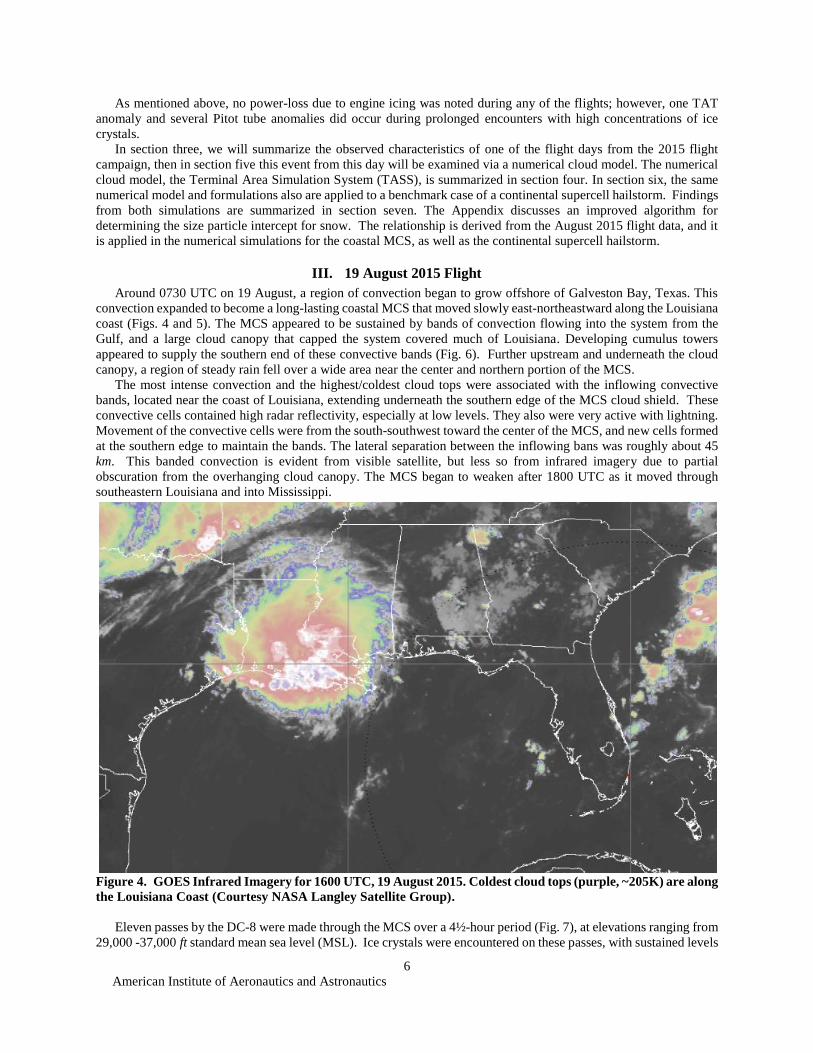
American Institute of Aeronautics and Astronautics
6
As mentioned above no power-loss due to engine icing was noted during any of the flights however one TAT
anomaly and several Pitot tube anomalies did occur during prolonged encounters with high concentrations of ice
crystals
In section three we will summarize the observed characteristics of one of the flight days from the 2015 flight
campaign then in section five this event from this day will be examined via a numerical cloud model The numerical
cloud model the Terminal Area Simulation System (TASS) is summarized in section four In section six the same
numerical model and formulations also are applied to a benchmark case of a continental supercell hailstorm Findings
from both simulations are summarized in section seven The Appendix discusses an improved algorithm for
determining the size particle intercept for snow The relationship is derived from the August 2015 flight data and it
is applied in the numerical simulations for the coastal MCS as well as the continental supercell hailstorm
III 19 August 2015 Flight
Around 0730 UTC on 19 August a region of convection began to grow offshore of Galveston Bay Texas This
convection expanded to become a long-lasting coastal MCS that moved slowly east-northeastward along the Louisiana
coast (Figs 4 and 5) The MCS appeared to be sustained by bands of convection flowing into the system from the
Gulf and a large cloud canopy that capped the system covered much of Louisiana Developing cumulus towers
appeared to supply the southern end of these convective bands (Fig 6) Further upstream and underneath the cloud
canopy a region of steady rain fell over a wide area near the center and northern portion of the MCS
The most intense convection and the highestcoldest cloud tops were associated with the inflowing convective
bands located near the coast of Louisiana extending underneath the southern edge of the MCS cloud shield These
convective cells contained high radar reflectivity especially at low levels They also were very active with lightning
Movement of the convective cells were from the south-southwest toward the center of the MCS and new cells formed
at the southern edge to maintain the bands The lateral separation between the inflowing bans was roughly about 45
km This banded convection is evident from visible satellite but less so from infrared imagery due to partial
obscuration from the overhanging cloud canopy The MCS began to weaken after 1800 UTC as it moved through
southeastern Louisiana and into Mississippi
Figure 4 GOES Infrared Imagery for 1600 UTC 19 August 2015 Coldest cloud tops (purple ~205K) are along
the Louisiana Coast (Courtesy NASA Langley Satellite Group)
Eleven passes by the DC-8 were made through the MCS over a 4frac12-hour period (Fig 7) at elevations ranging from
29000 -37000 ft standard mean sea level (MSL) Ice crystals were encountered on these passes with sustained levels
American Institute of Aeronautics and Astronautics
7
at high concentrations measured on at least two of the passes The peak ice water content measured by IKP-2 was 23
g m-3 with the longest duration having 1 g m-3 or greater persisting over a 114 km path or during about 10 min of flight
Figure 5 Low-level radar reflectivity from NEXRAD Radar (left column) compared with visible satellite
imagery (right column) at 1600 UTC (top row) and 1645 UTC (bottom row) All four plots are of the same
spatial scale Banded convective lines are feeding into the MCS from the Gulf of Mexico
Figure 6 Lines of towering cumulus feeding into southern end of the Louisiana MCS and growing upward
through the overhanging cloud canopy Photographs from window of DC-8 courtesy of Stephanie DiVito (FAA)
American Institute of Aeronautics and Astronautics
8
Highest ice water concentrations seem to be located in the southern portion of the MCS where the convective
lines were feeding into the system The DC-8 encountered persistent regions of significant ice water concentration in
the two flight-legs along the Louisiana Coast but less so in other regions (Fig 7) Only weak concentrations were
measured in the northern regions and near the center of the cloud system where steady rain occurred
Although no engine irregularities were detected other events did happen Anomalies in airspeed due to icing of
both Pitot tube systems occurred during penetration of HIWC conditions Also during these ice crystal encounters
the DC-8 experienced 1) view of snow specks or ice particles hitting windows and being sucked into the engines 2)
IFR conditions 3) rime ice developing on both the Pitot tube and TAT probe outside the cockpit window 4) light
turbulence and 5) benign values of RRF appearing on the ship radar
This flight-day is of interest because of the storm systems structure which is unlike the MCS from the Darwin
Australia campaign that we have recently simulated10 In addition National Weather Service NEXRAD radar
(ground-based WSR-88D)16 data is available to supplement our analysis During many of the flights that were on other
days the DC-8 was not in range of ground-based radars
A scatter plot of the short-range (1micros pulse) airborne radar reflectivity factor vs measured ice water content for 19
August is shown in Fig 8 Values for IWC are measured by the IKP-2 and averaged over five seconds The criteria
for determining the RRF is that it must be detected within 1-km of the DC-8 Additionally it must be detected within
an altitude range of plusmn 150m (500 ft) of the flight path and laterally within the antenna azimuth angle of a beam width
(plusmn2 degrees) These criteria were put into place to best represent the RRF of the air that is actually encountered by the
aircraft Note that median values for RRF asymptote to near 20 dBZ when IWC increases to greater than 1 g m-3
Additionally there is a large range of scatter exists between RRF and IWC Although not shown plots from each of
the other days appear very similar having low values of RRF and a weak relationship to ice water content This would
suggest that RRF alone may be an unsuitable measurement parameter for detecting HIWC
An example from the display of the airborne research radar is shown in Fig 9 as the aircraft heads northeastward
across the Louisiana Coast This plot is sampled at a time when high ice water concentrations were being encountered
and the aircraft was passing over convective bands within the southern region of the MCS With level tilt the radar
displays mostly green (less than 30 dBZ) over a wide area Areas of higher reflectivity are evident with the downward
tilted scan and are associated with the convective bands crossing obliquely to the flight path Distinguishable radar
signatures for HIWC encounters do not seem to stand out
Figure 7 Flight path of DC-8 and measured ice water concentration from Ice Kinetic Probe for 19 August
2015
American Institute of Aeronautics and Astronautics
9
Figure 8 Peak short-range radar reflectivity factor (within 1-km of aircraft) vs ice water content measured by
IKP-2 for 19 August The median ice water concentration is represented by the red curve
Figure 9 One-hundred kilometer scan of radar reflectivity factor from the NASA Airborne Radar at 1634
UTC during HIWC encounter on 19 August for level tilt (left) and -4o tilt (right) Range rings every 5 km The
aircraft is at 885 km (29kft) MSL on an ENE baring just north of the Louisiana Coast
IV Numerical Model
A three-dimensional time-dependent numerical cloud model is used to investigate and shed further light on the
characteristic of this HIWC producing storm system Numerical simulations are performed with NASArsquos Terminal
Area Simulation System (TASS)171819 which has a history of being used to study microburst windshear 20212223
convection induced turbulence2425 aircraft wake vortices26272829 atmospheric boundary layer turbulence303132
tornadoes33 and severe convection34 Recently it has been applied to the study of HIWC such as a MCS convective
line observed during a HAIC-HIWC flight campaign at Darwin Australia10 The numerical model has prognostic
equations for velocity potential temperature pressure and water substances (water vapor cloud droplet water rain
water cloud ice crystal water snow and hailgraupel) TASS also has over 60 cloud microphysical submodels for
cloud and precipitation development The TASS formulation includes all three-phases of latent heat exchanges for
water and has a subgrid-turbulence closure formulation based on Vreman35 Boundary conditions can be periodic
American Institute of Aeronautics and Astronautics
10
open or closed and in combination The surface boundary is assumed flat and can represent either ocean or a flat
ground The impermeable surface boundary is nonslip with a parameterization for surface stress based on Monin-
Obukhov similarity theory36 Initiation packages are available for triggering cumulus convective systems turbulence
microbursts and aircraft wake vortices A summary of the salient characteristics of TASS are in Table 2 The TASS
model has over a 30-year history of supporting NASA programs37
Table 2 Salient Features in TASS
Ambient conditions initialized with atmospheric sounding
Arakawa C-grid staggered numerical mesh
Bulk parametrizations for cloud microphysics (over 60 sub-models)
Compressible time-split formulation
Efficient and accurate conservative numerical schemes with little or no numerical diffusion
Ground-stress based on Monin Obukhov Similarity Theory
History of application to aviation weather and safety problems
Initialization packages for convective storms microbursts turbulence planetary boundary layer and aircraft wake vortices
Large Eddy Simulation with subgrid scale turbulence closure
Liquid vapor and ice phase microphysics
Massively parallel interface scales efficiently with multiple processors as used on high-performance supercomputer clusters
Meteorological framework
Model simulations validated with field data and theoretical solutions
Monotone upstream-centered schemes for water substance
NonBousssinesq equation set
Nonreflective boundary conditions for open boundaries
Option of either open or periodic lateral boundaries
Option for either periodic or impermeable top and bottom boundaries
Prognostic equations for velocity pressure potential temperature dustinsects and water substance
Storm-tracking movable grid domain
Variable time step to ensure CFL criteria for numerical stability
Vreman subgrid turbulence closure model with modification for stratification and flow rotation
Water substance represented by water vapor liquid cloud water rain cloud ice snow and hailgraupel
Wet and dry growth for hail and snow
A Numerical Approximations
The TASS model equations are discretized using quadratic-conservative fourth-order finite-differences in space
for the calculation of momentum and pressure fields38 and the third-order upstream-biased Leonard scheme39 is used
to calculate the transport of potential temperature and water vapor A Monotone Upstream-centered Scheme for
Conservation Laws (MUSCL)-type scheme after van Leer4041 is used for the transport of water substance variables
Such a scheme is mostly free of negative water production from numerical error The Klemp-Wilhelmson time-
splitting scheme42 is used for computational efficiency in which the higher-frequency terms are integrated by
enforcing the CFL criteria to take into account sound wave propagation due to compressibility effects The remaining
terms are integrated using a larger time step that would be appropriate for anelastic and incompressible flows The
Adams-Bashforth scheme is assumed for time differencing of momentum and pressure for both large and small time
American Institute of Aeronautics and Astronautics
11
step approximations The TASS model is programmed in FORTRAN and operates efficiently on massively-parallel
computer architectures using Message Passing Interface (MPI) library calls
The numerics in TASS are very accurate highly efficient and nondissipative The integrity and accuracy of the
numerical and core dynamics is evaluated by performing a number of validation tests These include validation of
numerical simulations with special cases for analytical and existing high-order numerical solutions such as Beltrami
flow4344 compressible Taylor-Green Vortex454647 solutions and other test cases48 TASS has been found to achieve
high accuracy and efficient timing in these comparison tests Furthermore to ensure continued accuracy and fidelity
simulations from TASS are performed and evaluated against several baseline cases following any modification to
either the software or operating system These tests are designed to test most components and maintain efficiency
robustness and accuracy of the model
B Cloud Microphysics
TASS has over 60 bulk cloud microphysical submodels similar to those used by Lin et al49 and Rutledge and
Hobbs50 The autoconversion of cloud droplets into rain is based on drop growth studies by Berry and Reinhardt5152
and allows for differences in cloud droplet sizes usually found between continental and maritime locations17 Rain is
assumed to have an inverse-exponential drop distribution with an intercept that increases with rainwater
concentration53 in accordance with data measured by Sekhon and Srivastava54
The prediction of ice particles are divided into three different categories 1) ice crystal water mdash which represents
small hexagonal ice crystals 2) Snow mdash which represents larger precipitating ice particles and 3) hail (or graupel)
mdash which represents even larger more dense particles that are produced from freezing rain drops and riming snow
particles The ice crystal water is assumed to have a monodispersed particle size that is limited to diameters no greater
than about 200 microm These particles are represented by hexagonal plates have little fall velocity and grow primarily
by diffusion of vapor The snow category assumes spherical particles that have an inverse exponential size distribution
The size distribution intercept for snow Nos increases with decreasing temperature and snow water content The
relationship for Nos is developed from particle size distribution (PSD) data collected during the 2015 Florida flight
campaign and is described with more detail in the Appendix A category for hail and graupel particles also assume
an inverse exponential size distribution but with a smaller intercept and a larger particle density than for snow Wet
and dry growth for hail follows the formulation in Musil55 Several of the key parameters assumed for the particle
distributions are summarized in Table 3
Radar reflectivity factor is diagnosed in TASS based on the predicted water content and the assumed particle
distributions These relationships for RRF use the same particle distributions that are assumed in the microphysical
submodels The approach assumes Rayleigh scattering and is based on Smith et al56 For example the radar reflectivity
factor for rain is
119937119929 = int 119925(119915119929)infin
120782119915119929120788119941119915119929
The particle size distribution can be effectively represented by an inverse exponential distribution as
119925(119915119929) = 119925120782119929119942minus120640119915119929
where NOR is the intercept of the drop size distribution and λ is the slope The contribution of radar reflectivity factor
from rainwater can be determined with the relationship for NoR as assumed in deriving the microphysics used in TASS
(Table 3)
ZR [ mm6m3] = 94 x 103 Mr1468
where spherical drops are assumed and Mr is the rainwater content in g m-3 The radar reflectivity factor for ice particles consider the dielectric factors for ice and water and depend upon
whether the particle is undergoing either wet or dry growth For example the contribution to radar reflectivity factor
for ldquodryrdquo snow adjust for the melted diameters is
119937119930 =|119922119920|
120784
|119922119934|120784 120633119930120784
120633119960120784 int 119925(119915119930)
infin
120782119915119930120788119941119915119930 (1)
American Institute of Aeronautics and Astronautics
12
The values assumed for the dielectric factors are for wavelengths employed in weather Radars57 The contribution to
RRF from hailgraupel ice crystals and cloud droplets are computed similarly For ldquowetrdquo hail the contribution is
adjusted for Mie scattering as in Smith et al56
Table 3 Key relationships and assumptions in TASS Microphysics
Category Size Distribution and
Intercept (m-4)
Particle Density ( )
Comment
Liquid Cloud Water
Monodispersed
1000 kg m-3
NCD number of droplets per volume is an input
Rain Inverse exponential
NOR = 225 x 107 M
R
0375
1000 kg m-3
Intercept increases with rainwater content
MR (g m
-3)
Cloud Ice Crystal Water
Monodispersed
Particle mass (kg) =
01758 Dic
22
Hexagonal plates Diameter mostly lt 200 microm
Snow Inverse exponential
NOS = 10(744 ndash 00217 Tc+ X)
where
X = Ms [1053-M
s (015-
0004Ms )]
for 4oC gt Tc gt -55
oC
100 kg m-3
if
Tc lt -12 oC
Ramping to 150 kg m-3
at
Tc gt 0 oC
Intercept increases with decreasing temperature
and increasing snow
concentration Ms (g m
-3)
HailGraupel Inverse exponential Intercept is an input
parameter
Either 450 kg m-3
if graupel or
900 kg m-3
if hail
Intercept decreases with temperature when Tcgt 0oC
V Numerical Simulation of 19 August Case
In this section the numerical simulation from the 19 August case is presented to help better understand the
characteristics of this system Comparisons with measured data are presented to substantiate the credibility of the
numerical simulation
A Configuration
In modeling the HIWC conditions associated with this convective system an approach similar to that used in the
Darwin HIWC simulation10 is used The domain of the model simulation is defined to represent a section of the MCS
rather than the full volume surrounding the weather system Specifically the modelrsquos computational domain is
specified about one of the inflowing lines of convection (Fig 10) Periodic lateral boundary conditions are assumed
on the domain boundaries parallel to the convective line and open lateral boundary conditions assumed on the ends
This configuration allows the simulated line to interact as if identical parallel lines exist on either side This includes
the interaction of the canopy outflow with the adjacent convective lines via the periodic boundaries The domain also
is rotated 21o to align the model y-axis with the direction of the low-level shear vector This results in the model
domain being oriented along the convective line since observed convection often orients itself in a line along the low-
level shear vector
The domain size and resolution (Table 4) is chosen to simulate the physics adequately and to resolve the essential
three-dimensional scales of motion The domain width of 45 km is based on the typical distance separating the
inflowing convective lines The grid size is chosen to concentrate the model grid points into a 45km x 150km area
American Institute of Aeronautics and Astronautics
13
The assumed grid size is the same in all three
directions (150m) and is small enough to allow the
resolution of important thermally-driven scales of
motion
The atmospheric sounding used as input is
extrapolated from an operational weather forecast
model at a location just upstream from the system
This sounding (Fig 11) possess strong convective
instability and deep levels of moisture This sounding
also indicates a tropopause at 14km MSL with a
temperature of about -62oC or 211K Convective
indices58 computed from the sounding indicate strong
convective instability with a lifted index of about -6oC
and CAPE = 3400 J kg-1 The melting level is at
4900m MSL
The initial state of the numerical simulation is
horizontally homogeneous and varies vertically
according to the input sounding shown in Fig 11
Convection is initiated by an artificial thermal
impulse A cool pool of air that resides near the
surface over much of Louisiana and underneath the
MCS is ignored for the initial and boundary
conditions The boundary conditions for the ground
are representative of a smooth ocean surface with
constant temperature Other input parameters for the
simulation are representative of a tropical oceanic
environment (Table 5) The simulation is integrated
over a 4-hour period with convection occurring
through the full period In our simulations time (t) is in reference to time of initiation and values for the x and y
coordinates are in reference to the initial triggering impulse
B Results
The numerical simulation generates a long-lasting system with a convective line oriented in the direction of the
low-level shear vector of the environmental winds The cyclic (ie periodic) boundary conditions on the left and right
sides of the domain account for the effect of multiple lines including the interaction between the lines The type of
convection is multicellular11 with overshooting tops penetrating through the tropopause by about 600 m The system
produces persistent HIWC conditions at storm upper levels within an expanding cirrus shield fed from the multi-
Figure 11 Skew-T diagram representing initial
environmental profiles for 19 August 2015 case
Modified from sounding extracted from an operational
weather model forecast at 1400 UTC at location
upstream from the MCS (29N 912W)
Figure 10 Model Domain size relative to MCS
Table 4 Domain Size and Resolution
Domain Parameter Physical Dimension
Lateral dimensions (X Y) 45 km x 150 km
Vertical dimension (Z) 186 km
Lateral grid spacing 150 m
Vertical grid spacing 150 m
Computational grid ~39 x 10
6
grid points
Table 5 Initial Parameters
Cloud base height 625 m (942 mb)
Cloud droplet number density Ncd 75 droplets cm-3
HailGraupel particle size distribution intercept Noh
4 x 10⁵ m-4
American Institute of Aeronautics and Astronautics
14
cellular convection A comparison of the low-level radar reflectivity factor from the model simulation with the
observed NEXRAD reflectivity is shown in Fig 12
Figure 12 Comparison of low-level RRF between NEXRAD (left) and TASS (right) Observed NEXRAD
for Louisiana coast at 1645 UTC Simulated RRF at 4km altitude and 3hr 45min Outline of TASS domain
shown (90 km x 150 km)
Updrafts within the convective line generate precipitation and carry snow particles and ice crystals to the upper-
regions of the troposphere At upper levels the expanding outflow coalesces with the upper-level anvil outflow from
adjacent lines to form a large overhanging canopy (Fig 13) The general comparison between observations and
numerical simulation are summarized in
Table 6
Horizontal cross-sections at two
altitudes for RRF and IWC are shown in
Figs 14 and 15 The chosen altitudes
represent the two flight altitudes for the
DC-8 during each of two passes when
persistent IWC was measured The timing
of the slices are at a model time of
3hr45min (from the start of initialization)
and represent a time when the simulated
system has reached a mature state Profiles
are extracted along the dashed line shown
in the figures and are compared to that
measured by the DC-8 (Fig 16)
In Fig 14 the numerically simulated
ice water concentration (ice crystal snow
and graupel water combined) as well as the
RRF are shown at flight level 29 kft (8850 m) Peak ice water concentrations exceeding 3 g m-3 can be found within
small areas associated with the convective updraft turrets Larger areas with a width of about 40km exceeded 1 g m-3
Radar reflectivity factor values are generally less than 30dBZ and would appear green on the weather radar display of
most aircraft Locally higher values of RRF were found within the strong updraft cores that carry graupel and other
ice particles The RRF in Fig 14 does show large areas of low RRF but not as uniform as from the flight radar (cf
Fig 9) A more appropriate comparison would be between the RRF observed by the DC-8 with a simulation of its X-
band radar using the TASS fields as input
Figure 13 Simulated three-dimensional cloud surface viewed
from above and from south-southwest
American Institute of Aeronautics and Astronautics
15
Table 6 Comparison of general features between observed and numerically simulated for 19 August 2015 case
Feature Observed Simulated with TASS
Orientation of convective lines SSW-NNE with 45 km separation between lines
SSW-NNE with 45 km separation between lines
Cloud top elevation ~14-15 km 146 km
Coldest cloud top temperature ~200 K 203 K
Cell movement from 210o at 10 ms 221o at 11 ms
Direction of anvil canopy expansion from Southwest Southwest
Convective line movement from 290o at 6 ms 291o at 45 ms
System lifetime gt 10 hrs gt 4 hrs
Width of area with RRFgt20 dBZ at cruise altitudes
gt 50 km 40 km
At a slightly higher altitude (Fig 15) regions with HIWC cover smaller areas and have lower values of RRF This
is consistent with the measurements from the DC-8 which encountered shorter durations of IWC greater than 1
g m-3 and detected lower values of RRF after changing to a 5kft higher altitude on a subsequent pass through the
active regions near the Louisiana coast
Figure 16 shows a comparison of measured and model-extracted profiles for RRF and IWC The DC-8 flight
profiles relative to the MCS are shown in Fig 17 The TASS profiles are extrapolated at the two different altitudes
and headings flown by the DC-8 and are compared with values measured by the DC-8 At the lower elevation both
the TASS and DC-8 profiles indicate a nearly steady RRF of about 20-25 dBZ and IWC mostly between 1- 25 g m-3
At the higher elevations both TASS and DC-8 show consistent magnitudes of variation with the RRF varying between
0 to 20 dBZ and the IWC mostly remaining below 05 g m-3 Both profiles at the higher elevation do show a small
region where IWC approached 2 g m-3 Although peak values and duration of encounters seemed similar in magnitude
the variability of RRF and IWC appears greater in the modeled profiles
In Fig 18 vertical cross-sections of the simulated RRF and IWC fields are taken along the assumed flight path in
Fig 14 Note that large regions of IWC greater than 15 g m-3 (orange) extend over a large region along and below the
lower-altitude flight path Peak values occur between altitude ranges of 75-95 km AGL and drop off significantly
above 10 km AGL The corresponding RRF shows larger values below the melting level (around 5 km AGL) and very
weak values above 10 km MSL Also note that regions with significant IWC can extend above regions with low or no
detectable RRF near the ground
In summary a persistent coastal MCS system with HIWC is numerically simulated and its results compared with
data from the 2015 Florida Radar flight campaign The system is sustained by bands of convection inflowing from the
Gulf of Mexico and is capped by a large canopy cloud consisting of mostly ice crystals The simulation showed that
the coalescence of the expanding anvils from the convective cells resulted in a cloud canopy that may obscure the
banded structure and other low-level features from detection with satellite The model simulated cloud top elevations
and movement of cells appear similar to observations Largest concentrations of ice water were found in the simulation
between 75 and 95 km (25kft-31kft) MSL where environmental temperatures were between -19oC to -33oC The
range of elevations with the largest RRF were between the surface and 6km (20 kft) MSL The TASS-extracted profiles
compare reasonably with the measurements from DC-8 although some differences in variability were noted
American Institute of Aeronautics and Astronautics
16
Figure 14 Simulated RRF (left) and IWC (right) from TASS simulation at an altitude of 8850m (flight level
29kft) and 3hr and 45 min The TASS IWC field is the sum of all ice water (ice crystal water + snow + graupel)
Figure 15 Same as Fig 14 but at 10335m (flight level 34 kft)
American Institute of Aeronautics and Astronautics
17
Figure 16 Comparison of RRF and IWC extracted along flight profiles shown in Figs 14 and 15 (dashed
lines) with those measured by the DC-8 (solid lines) Top row at an altitude of 8850m bottom row at 10350m
Figure 17 Two of the DC-8 legs with longest duration of IWC
Track of DC-8 superimposed on 1645 UTC GOES-13 Infrared
satellite imagery (Courtesy NASA Langley Satellite Group)
American Institute of Aeronautics and Astronautics
18
Figure 18 Vertical cross sections of RRF (top) and IWC (bottom) extrapolated from the numerical
simulation along the flight profile shown in Fig 14 Vertical position of both flight paths shown by dashed line
Altitudes are AGL
The numerical simulation does not capture the region of stratified precipitation that lies downstream from the
inflowing convective lines However the DC-8 flights did not encounter regions of HIWC when they overflew this
region It appears likely that the rain in this area was produced by moisture from the dissipation of the convective cells
and the overrunning of the cool surface dome by the moist southerly air currents A next-generation simulation would
need to include the horizontal variation of temperature and wind into the simulation in order to capture these effects
VI Numerical Simulation of Continental Supercell Hailstorm
In this section the numerical simulation of a continental supercell hailstorm is presented The purpose of this
simulation is to validate the robustness of the microphysics used in TASS and better understand differences in HIWC
production between continental supercell storms and subtropical MCS convection Validation parameters include 1)
production of large hail 2) size of hail swath 3) radar bounded weak echo region 4) supercell features 5) storm
motion 6) size and intensity of quasi-steady updraft 7) size and maximum value of radar echo and 8) duration In
this simulation we will verify the validity of the simulation by comparing our solutions with observed data In
addition this case will be analyzed for its potential in producing HIWC and compared with the previous case of
summertime coastal convection
This case has been simulated in the past with one of the first versions of TASS using a relatively coarse mesh
Even at this earlier stage of TASS development the simulation was able to capture many of the stormrsquos observed
features5934
A Description of Observed Case
On 2 August 1981 a very large and severe hailstorm moved across Southeastern Montana The storm was observed
during its mature phase with ground-based Doppler radars and with research aircraft as it moved through a network
of field instruments during the Cooperative Convective Precipitation Experiment60 (CCOPE) The storm quickly
developed many classical features of a supercell hailstorm It veered to the right of the environmental winds and
persisted for over 5 hours while leaving a wide swath of hail The storm was reported to have an intense quasi-steady
updraft with cyclonic rotation a low-level radar hook echo signature a mid-level bounded weak echo region (BWER)
signature (same as radar echo vault) damaging winds a broad swath of 1-3 cm diameter hail with some sizes as large
American Institute of Aeronautics and Astronautics
19
as 10 cm a mesolow or mesocyclone with a peak pressure drop of at least 6mb and a peak RRF between 65-75
dBZ61626364 The primary updraft of the storm was reported to be over 14 km wide and was located within the BWER
A research aircraft flew within the updraft at an altitude between 6 km and 75 km MSL they found nearly adiabatic
conditions with updraft speeds greater than 50 m s-1 liquid water droplet concentrations of up to 6 g m-3 and the
absence of precipitation-sized particles65 The lack of larger particles explained the very low magnitudes of RRF within
the BWER Hail was penetrated by the research aircraft on the western edges of the updraft in association with the
high reflectivity regions Weisman et al66 reported that the storm produced at least one funnel cloud and that some
damage reports were ldquosuggestiverdquo of tornadic activity Surface wind speeds were estimated between 50 to 100 mph
(20 to 45 m s-1)63
A special rawinsonde sounding was launched near the storm (Fig 19) and indicated an environment very favorable
for intense convection Convective indices
calculated from the sounding exhibited a CAPE of
almost 3500 J kg-1 and a lifted Index of -10oC
The sounding also indicated a tropopause height
of 109 km MSL (~99 km AGL) with a
temperature of -475oC and an equilibrium level
at 198 mb (123 km MSL) with a temperature of -
517oC According to the both the sounding and
aircraft observations the cloud base temperature
and height were about 136oC and 26 km MSL
respectively63 The ground was slightly less than
1km above sea level and varied somewhat with
location The wind profile for the sounding
exhibited a strong magnitude of helicity6768 and
vertical shearing of the environmental wind High
values of both helicity and CAPE are indicative of
supercell and tornadic storm environments The
presence of dry environmental air at storm mid-
levels likely inhibited any strong tornado
formation (eg Proctor et al33)
B Configuration
In numerical modeling of this system we apply the
same version of the TASS model as in the Coastal-MCS
case Differences are only due to grid and domain
configuration boundary conditions input sounding and
several input parameters that define the continental
aspects of the cloud droplets and the hail size
distribution All are discussed below
The domain is size is defined to be 150 km x 150 km
in the horizontal and 20 km in the vertical (Table 7) An
evenly spaced grid size of 200 m is assumed Open
lateral boundaries conditions are applied at all lateral
boundaries The ground surface is assumed flat and no
terrain features are included The domain uses the
TASS modelrsquos internal tracking algorithms17 in
order to move the grid with the lateral translation of
the storm
The initial state profiles for temperature
pressure wind and humidity are horizontally
uniform but vary vertically according to the input
sounding shown in Fig 19 Values representative of
contental Great-Plains systems are assumed to for
the cloud droplet concentration and for the hail size
distribution intercept parameter (Table 8)
Figure 19 Skew-T diagram representing environment for
2 August 1981 Special sounding observed near Knowlton
MT at 2356 UTC Environmental wind hodograph
inserted at bottom left
Table 7 Domain Size and Resolution
Domain Parameter Physical Dimension
Lateral dimensions (X Y) 150 km x 150 km
Vertical dimension (Z) 20 km
Lateral grid spacing 200 m
Vertical grid spacing 200 m
Computational grid ~56 x 10
6
grid points
Table 8 Initial Parameters
Cloud base height (AGL) 1700 m (740 mb)
Cloud droplet number density Ncd 800 droplets cm-3
HailGraupel particle size distribution intercept Noh
2 x 10⁴ m-4
American Institute of Aeronautics and Astronautics
20
The major diffences between the initial conditions of this case and the coastal MCS case are that this case
represents a more continental environment with stronger vertical wind shear less moisture but greater instability
C Comparison of Simulation with Observations
The numerical simulation is initiated at time zero by introducing a thermal impulse and integrating over 4 hours
of time The simulation produces a supercell hailstorm and captures many of the features observed in the real storm
These include large hail wide hail swath funnel cloud with damaging surface wind 15 km wide quasi-steady updraft
surrounded at storm-mid-level by a radar echo vault or BWER a radar hook echo signature right-rear quadrant gust
front massive overshooting tops and a large spreading anvil As can be see in Table 9 scales and intenisties match
very well between the observed and simulated event The simulated updraft velocity at 65 km MSL of 55 m s-1 matches
the peak value measured by a research aircraft that penetrated the storm at the same level As found from the aircraft
measurments the updraft core was nearly adiabatic with little or no precipitation The model simulation as in the
observational studies found most of the hail to be on the western and nortwestern edges of the primary storm updraft
Table 9 Comparison of observations with TASS for 2 August 1981 Supercell Hailstorm
Features Observed TASS Simulated Anvil Extent Downstream from Updraft
(based on Radar Echo) gt200 km gt150 km
Anvil Extent Upstream from Updraft gt20 km gt60 km
BWER Diameter ~75 km ~8 km
BWER Vertical Extent 10 75 km MSL 12-14 km MSL
Gust Front Location SW Flank SW Flank
Peak Gust Front Wind Speed gt20 ms 25 ms
Typical Hail Diameter at Surface 1-3 cm peak median diameter 2 cm
Hail Shaft Location Relative to Center of BWER 3-4 km West 4-6 km WNW
Width of Hail Swath 20-30 km 225 km
Supercell Lifetime gt 5 hrs gt 4 hrs
Persistent Low-Level Radar Hook Echo yes Yes
Maximum Liquid Cloud Water Content 65 g m-3 55 g m-3
Surface Pressure Drop 6 mb Mesocyclone 4 mb tornado 21 mb
Peak Rainfall Accumulation 30-35 mm 25 mm
Peak Radar Reflectivity Factor 75 dBZ 726 dBZ
Storm Movement (development stage) 260 at 10 ms 250 at 12 ms
Storm Movement (supercell stage) 282 at 18 ms 280 at 16 ms
Storm Top Overshoot above EL 3-4 km 5 km
Updraft Diameter 14-17 km 15 km
Max Updraft Velocity at 65 km MSL 53 ms 55 ms
Diameter of 20 dBZ Echo at 12 km MSL 45 km 45 km
Peak Surface-Level Gusts East of Updraft gt25 ms 30 ms
Radar Echo Top 16 km MSL 18 km MSL
Tornadoes Funnel cloud sighted Yes western side of mesocyclone
Peak Surface Wind Damage F1- wind damage (estimated 33-50 ms)
56 ms
Maximum Altitude of 10 dbZ Contour in BWER 6-8 km MSL 65 km MSL
American Institute of Aeronautics and Astronautics
21
Supercell environments often produce tornadoes or familes of tornadoes and a funnel cloud with surface wind
damage was reported with this system The funnel cloud that was produced in the numerical simulation was
intermittent and dissiapted when it moved into the cooler dryer air underneath the hail and rain shafts Tornado
formation in this simulation showed similar characteristics to those studied in an earlier paper where the presence of
dry mid-level air acts to weaken or suppress tornado formaition in supercell environments33
The time evolution of the area with RRF greater than 55 dBZ at an elevation of 5 km MSL (blue) and the peak
RRF anywhere in the storm (red) is shown in Fig 20 The peak RRF from the simulation matches the observations
very well For the area with RRF greater than 55 dBZ both observation and TASS show a ramp up in the first two
hours of the stormrsquos lifetime but the
simulation shows this area to be smaller
than detected by ground-based radar
A comparison of the supercell structure
from TASS with measurements from
ground-based radar are shown in Figs 21
and 22 Two horizontal levels of RRF are
shown one at 10 km MSL and the other at 4
km MSL The TASS simulation reproduces
many of the observed features and supercell
signatures including the BWER (ie radar
echo Vault (V)) the radar hook echo and
the radar echo streamer The scale of the
area covered by each intensity of RRF are
similar between TASS and observed as
well One contrast however is that the high-
reflectivity area within the hook echo region
appears larger in the observation than in the
simulation The area of highest reflectivity
which is west and northwest of the BWER
is associated with large hail in both
observation and simulation
In Fig 23 a vertical cross-section along
x-z coordinates is taken through the middle
of the BWER Again both the simulation and observation show similar features similar intensities and similar spatial
scales The BWER or radar Vault is clearly present in the simulation and extends deep into the storm The BWER
is located within the intense storm updraft and is produced by a lack of significant precipitation-sized particles
D HIWC Characteristics in Simulated Storm
The Montana supercell with its quasi-steady large diameter and intense updraft generates large volumes of ice
crystals that are transported into the upper regions of the troposphere Increasing wind speeds with height which is a
characteristic of supercell environments quickly transports many of the ice particles downstream within a large
expanding anvil cloud Hail and larger ice particles are also carried up to high altitudes by the strong updrafts but fall
out relatively close-by due to their significant fall velocities Therefore large values of RRF can be found at storm
upper-levels within proximity to the supercell updraft The RRF drops-off with distance from the updraft as the larger
particles fall out and the remaining smaller particles are carried downstream
A graphical representation of the cloud and precipitation fields from TASS is show in Fig 24 Overshooting tops
which are above the predominant supercell updraft can penetrate several kilometers into the stratosphere A large
anvil cloud spreads mostly downstream from the overshooting tops due to the strong westerly winds beneath the
tropopause (cf Fig 9) This anvil cloud covers many square kilometers and forms a large overhang of cloud material
downstream from the storm updraft Due to the intensity of the updraft some the anvil material is transported counter
to upper-level winds and produces a forward overhang upstream from the storm updraft
The coldest cloud tops (Fig 25) are associated with the overshooting tops above the intense storm updraft Cloud
tops at temperaturesheights near the equilibrium level expand over a large area downstream from the overshooting
tops Obviously in Fig25 the anvil expands northeastward beyond the boundaries of the model domain
Figure 20 Time evolution of the maximum RRF anywhere
in the storm (red) and the cross-sectional area of reflectivity
exceeding 55 dBZ at 5km MSL (blue) Observed values from
Miller et al63(solid) compared with TASS (dashed)
American Institute of Aeronautics and Astronautics
22
Figure 22 Same as Fig 21 but RRF at an elevation of 4 km MSL Left adapted
from Millerrsquos analysis of ground based Doppler radar right from TASS at
t=3hr07min
RRF (dBZ)
Figure 21 Horizontal cross-section of Radar reflectivity factor at an altitude of
10 km MSL Left adapted from Millerrsquos analysis of ground based Doppler radar62
right from TASS at t=3hr07min Both plots windowed to 50km x 50km area with
major tick every 10 km The Radar echo Vault or BWER identified with V
Figure 23 Same as Fig 21 but RRF along vertical west-east cross-section through
BWER Left adapted from Millerrsquos analysis of ground based Doppler radar right from
TASS at t=3hr07min Altitude in km AGL with major ticks every 1km along abscissa
American Institute of Aeronautics and Astronautics
23
Very similar features for the simulated Montana supercell storm can be seen in the observed visible satellite
imagery of the actual system (Fig 26) The overshooting tops are positioned near the southern end and the anvil
expands toward the north-northeast The horizontal dimension of the observed cloud anvil compared with the cloud
top depicted in Fig 25 are nearly identical
Figure 27 shows the simulated IWC and RRF along a horizontal cross-section taken at 10km MSL (9km AGL)
The size and shape of the system represented in the cross-section is consistent with the satellite imagery in Fig 26 In
Fig 27 most of the RRF greater than 20 dBZ is confined to area within a 50 km diameter centered about the primary
updraft and BWER Values of RRF between 15-20 dBZ cover large areas downstream for the overshooting tops
Figure 27 also shows vast areas with IWC greater than 1 g m-3 In fact areas with 1 g m-3 or greater can be found at
distances of up to 50 to 100 km away from the regions with the greatest storm RRF Our simulation seems to imply
that by avoiding the high reflectivity areas by 20 nautical miles (37 km) may not be sufficient for avoiding prolonged
HIWC exposures
Figure 24 Simulated cloud and precipitation surfaces within the full TASS domain Viewed from south
Figure 25 Cloud top temperatures from TASS at 3hr75 min (left) and 3hr45min (right) simulation
time Coldest temperatures associated with overshooting tops in southwestern quadrant of figure
American Institute of Aeronautics and Astronautics
24
To further explore the structure of the simulated storm
vertical cross-sections are extracted alone lines A-B and C-D
that that appear in Fig27 These cross sections are shown in
Figs 28 and 29 They also help illustrate where HIWC
conditions may be found relative to the storm
The cross-sections through A-B (Fig 28) are taken
northeastward through the storm updraft It shows strong
reflectivity surrounding the BWER and extending to the upper
levels of the storm High levels of IWC largely composed of
hail are brought to the ground on the southwestern side of the
storm updraft and at upper-levels surrounding the updraft
Aircraft routinely avoid these areas due to their high values of
RRF More of a factor to air traffic is that significant levels of
IWC that can be found over large areas within the cloud
canopy at great distances downstream from the stormrsquos high
reflectivity regions Furthermore the RRF within the canopy
are very low and could be undetectable with many airborne
weather radars
In Fig 29 a cross section is taken orthogonal to the
direction of the shearing anvil It is taken northwestward
between C and D along the edge of the areas with significant
IWC (Fig 27) This cross-section resides at least 70 km or
more from areas with high RRF Along this cross section IWC
greater 1 g m-3 can be seen to extend for over a 100 km length
The layer has a thickness that is several kilometers thick This
layer also consist of very weak RRF (lt 20 dBZ) and
underneath has no detectable radar reflectivity or precipitation
Both cross-sections show that a layer with HIWC can extend over large distances and with very weak RRF
Beneath this layer containing HIWC precipitation was rarely apparent and radar reflectivity not detectable One visual
queue sometimes recommended to pilots for helping to identify potential HIWC conditions is the presence of strong
to moderate RRF from rain beneath regions of HIWC This queue would not apply to a supercell storm such as this
This case of a continental supercell also demonstrates that HIWC risks may not be confined to just oceanic and
coastal MCS since regions of significant IWC may extend for large distances with little RRF
VII Discussion and Conclusion
Flight data and results from numerical simulations are analyzed to better characterize the HIWC threat for aircraft
and to improve our understanding of the relationship between HIWC radar and satellite signatures Flight
measurements with airborne radar and microphysical probes suggest that RRF alone may not be adequate for the
detection of HIWC conditions This fact also is reinforced from the numerical model simulations
The numerical simulations confirm that HIWC can be produced in contrasting environments In warm moist
coastal and oceanic environments large volumes of ice crystals can be pumped into the upper-troposphere by
regenerating convective plumes associated with a long-lasting system Cloud material carried in the upper-level
outflow from these plumes coalesces to form a large overhanging canopy and contain significant concentrations of
ice crystals Perhaps due to the weaker wind shear of these environments and the duration of the systems large
concentrations may accumulate over time
Our simulation of a large continental supercell shows it to have a large persistent and nearly adiabatic updraft
that also can pump large volumes of ice crystals in to the upper troposphere Vertical windshear with strong winds
aloft (which are an ingredient in producing supercells) can act to transport ice crystals over large areas We speculate
that the increase ventilation due to environmental wind shear may dilute the peak concentrations of IWC in supercells
Figure 26 Observed visible satellite imagery
from GOES-7 Northeastern Montana 2315
UTC 2 August 1981
American Institute of Aeronautics and Astronautics
25
Figure 27 Ice water content (left) and RRF (right) from TASS at an elevation of 10km MSL and 3hr45
min) simulation time Ice water content (g m-3) is sum of ice crystal snow and hail water content Units
for RRF are (dBZ)
Figure 28 Vertical cross section along A-B in Fig 27 Top is ice water content (g m-3) and bottom is RRF
(dBZ) Altitudes are above ground level
American Institute of Aeronautics and Astronautics
26
In our study the microphysics for snow is improved by using analyzed PSD data measured during the flight
campaign A new relationship is developed that relates the exponential size-distribution intercept for ice particles with
their water content In the past the value for the intercept has been assumed constant or a function of temperature
only The new relationship is a function of snow or ice water content as well as temperature and was used to improve
the microphysical submodels in TASS
The TASS model was then applied to contrasting types of convection and compared to available observations
This comparison seemed very good and demonstrated the model could be applied robustly to convection in different
types of environments Excellent results were achieved using only simple bulk parametrizations for microphysics
suggesting that models that are more complex may not be needed depending upon application The profiles of ice
water content and RRF extracted from the simulation compared reasonably well with the measurements by the DC-8
during penetrations of the coastal MCS although some differences in variability were noted The TASS model was
also used to simulate a specific supercell hailstorm with excellent comparison to measurements in terms structure
features scales and magnitudes
The numerical studies for both cases found that regions of significant IWC could extend above regions with little
or no RRF This would imply that moderate to high radar reflectivity might not always be underneath HIWC events
Yet to be investigated is the potential for HIWC detection using a combination of sensors and sources for
information (ie satellite and other weather data) Also unexplored is the ability to detect HIWC with advanced
airborne radar tools
Appendix Ice Crystal Size Distributions
Relationships between the ice crystal size distributions temperature and ice water content are needed for the
parameterization of microphysical submodels used in TASS These relationships could be useful in other applications
such as the understanding the radar reflectivity factor (RRF) due to ice crystals Dr Alexei Korolev processed the
particle size distribution (PSD) data69 from data collected at one-Hertz intervals during the DC-8 flights from a 2D-S
probe and a particle-imaging probe (PIP) The measured data was discretized into appropriate size bins and normalized
by the width of the corresponding bin This allowed for the direct comparison of the PSD data with different size
resolutions and common theoretical drop-size distributions (eg Marshall-Palmer70) The size resolution for the 2D-S
probe was10 μm and 100 μm for the PIP The range of particle measurements extends from 15 μm to 12845 mm The
Figure 29 Same as in Fig 28 but for position C-D in Fig 27
American Institute of Aeronautics and Astronautics
27
size of irregularly shaped ice particles as estimated from particle images may be defined in several different ways
The composite PSD data used the length of the particle parallel to the photodiode array commonly called Ly
An intercept (N0) and slope (λ) parameter were found from the data by using a least-squares method to fit an
exponential distribution through the measured PSD This was repeated for all times in a flight Relationships can then
be established for N0S vs ice water content (IWC) and atmospheric temperature
Our numerical modeling effort previously employed a relationship for Nos that is a function of temperature
only1017 Recall that our snow category represents the larger ice particles (excluding graupel and hail) and assumes
an inverse exponential size distribution whereas our cloud ice category only represents the smaller ice particles with
diameters less than about 200 um Using combined data measured from each day of the NASA deployment (Table 1)
and binning according to temperature a new relationship was determined for Nos that is a function of both temperature
and snow water content Ms
Log10 (Nos) = 744 ndash 00217 Tc +10526 Ms ndash 015 Ms2 +0004 Ms3 (A-1)
for Tcgt -55OC and Ms lt 4 g m-3
where Nos has units of m-4 Ms has units of g m-3 and Tc is temperature of the environment in centigrade The
relationship was fitted from the flight data as shown in Fig A1 and produces a larger intercept value for either colder
temperatures or increasing snow water content A higher intercept value translates into a distribution with overall
smaller particles lower radar reflectivity factor and slightly slower fall velocity Other parameterized microphysical
processes are affected by the assumption for Nos these include sublimation or deposition of snow particles and other
growth processes
Note that when Ms 0 the above relationship asymptotes to a relationship suggested by Woods et al71 who
derived their relationship from analyzing ice particles in wintertime precipitation occurring in the Pacific Northwest
Based on all ice particles they found the following relationship for No
Log10 (No ) = 753 ndash 00207 Tc (A-2)
Since their measured ice water contents ranged between 003 and 030 g m-3 it would have been difficult for them to
detect any dependency of No on ice water content
As a further check to the validity Eq (A-1) we compare the observed short-range RRF with the value estimated
from the measured IWC using the assumption of an inverse exponential size distribution with Eq (1) as
ZS [mm6m3] = 390 x 108 Ms175 Nos
-075 (A-3)
where the above assumes melted spherical particles and accounts for the differences in radar dielectric constants for
ice and water
The comparisons are shown in Fig A1 and illustrates the lack of correlation of radar reflectivity with snow water
concentration for values of snow water greater than about 1 g m-3
American Institute of Aeronautics and Astronautics
28
Figure A1 Ice particle distribution intercept NoS
vs ice water content for three temperature ranges
Data points derived from PSD distributions
measured during all 2015 DC-8 Flight Campaign
flights (ie Table 1) Blue curve represents medium
value Red curve is fit using Eq (A-1)
Figure A2 Radar reflectivity factor vs ice
water content for three temperature ranges
Data points of close-range RRF measured during
all 2015 DC-8 Flight Campaign flights (ie Table
1) Blue curve represents medium value Red
curve using Eqs (A-3) and (A-1)
American Institute of Aeronautics and Astronautics
29
Acknowledgments
This research is sponsored by the Advanced Air Transport Technology Project of NASArsquos Advanced Air Vehicles
Program The authors would like to acknowledge the contributing organizations that enabled the Florida HIWC Radar
Flight Campaign the FAA Aviation Research Division and Aviation Weather Division the NASA Aviation Safety
Program the Boeing Company Met Analytics Science Engineering Associates Environment Canada the National
Center for Atmospheric Research Honeywell and Rockwell Collins The authors also would like to thank Tom
Ratvasky (NASA Glenn Research Center) and Walter Strapp (Met Analytics) for their programmatic technical and
operational support and the NASA Langley Satellite Group for providing satellite images In addition thanks to
Alexei Korolev (Environment and Climate Change Canada) for processing the PSD data from raw data collected
during the flight test The numerical simulations were conducted using the Pleiades high-performance supercomputer
cluster of the NASA Advanced Supercomputing Division
References
1Mason JG Strapp JW and Chow P ldquoThe Ice Particle Threat to Engines in Flightrdquo AIAA 2006-206 doi10251462006-
206 2Mason JG and Grzych M ldquoThe Challenges Identifying Weather Associated with Jet Engine Ice Crystal Icingrdquo SAE
International 2011-38-0094 doi1042712011-38-0094 3Bravin M Strapp JW and Mason J ldquoAn Investigation into Location and Convective Lifecycle Trends in an Ice Crystal
Icing Engine Event Databaserdquo SAE International 2015-01-2130 doi1042712015-01-2130 4Addy HE Jr and Veres JP ldquoAn Overview of NASA Engine Ice-Crystal Icingrdquo SAE International 2011-38-0017
doi1042712011-38-0017 5Grandin A Merle J-M Weber M Strapp JW Protat A and King P ldquoAIRBUS Flight Tests in High Ice Water Content
Regionsrdquo AIAA 2014-2753 doi10251462014-2753 6Protat A and Rauniyar S Kumar VV and Strapp JW ldquoOptimizing the Probability of Flying in High Ice Water Content
Conditions in the Tropics Using a Regional-Scale Climatology of Convective Cell Propertiesrdquo Journal of Applied Meteorology
and Climatology Vol 53 November 2014 pp 2438-2456 doi101175jamc-d-14-00021 7Dezitter F Grandin A Brenguier JL Hervy F Schlager H Villedieu P and Zalamansky G ldquoHAIC (High Altitude
Ice Crystals)rdquo AIAA 2013-2674 doi10251462013-2674 8Houze RA Jr ldquoMesoscale Convective Systemsrdquo Review of Geophysics Vol 42 RG4003 2004 pp 1-43
doi1010292004RG000150 9Grzych M Tritz T Mason J Bravin M and Sharpsten A ldquoStudies of Cloud Characteristics Related to Jet Engine Ice
Crystal Icing Utilizing Infrared Satellite Imagerrdquo SAE International 2015-01-2086 doi1042712015-01-2086 10Proctor FH and Switzer GF ldquoNumerical Simulation of HIWC Conditions with the Terminal Area Simulation Systemrdquo
AIAA-2016-4203 doi10251462016-4203 11Houze RA Jr Cloud Dynamics Ed Academic Press 1993 573 pp doi101002qj49712051918 12FAA ldquoTurbojet Turboprop and Turbofan Engine Induction System Icing and Ice Ingestionrdquo February 2004 Advisory
Circular 20-147 doi104271510198 13Davison CR Strapp JW Lilie L Ratvasky TP Dumont C ldquoIsokinetic TWC Evaporator Probe Calculations and
Systemic Uncertainty Analysisrdquo AIAA 2016-4060 doi10251462016-4060 14Strapp JW Lilie LE Ratvasky TP Davison C and Dumont C ldquoIsokinetic TWC Evaporator Probe Development of
the IKP2 and Performance Testing for the HAIC-HIWC Darwin 2014 and Cayenne-2015 Field Campaignsrdquo AIAA 2016-4059
doi10251462016-4059 15Lilie LE Sivo CP and Bouley DB ldquoDescription and Results for a Simple Ice Crystal Detection System for Airborne
Applicationsrdquo AIAA 2016-4058 doi10251462016-4058 16Crum TD and Alberty RL ldquoThe WSR-88D and the WSR-88D Operational Support Facilityrdquo Bulletin of the American
Meteorological Society Vol 74 No 9 1993 pp 1669-1688 doi1011751520-0477
doi1011751520-0477(1993)074lt1669TWATWOgt20CO2 17Proctor FH ldquoThe Terminal Area Simulation System Volume I Theoretical Formulationrdquo April 1987 NASA CR-4046 18Proctor FH ldquoNumerical Simulation of Wake Vortices Measured During the Idaho Falls and Memphis Field Programsrdquo
14th AIAA Applied Aerodynamic Conference Proceedings Part II June 1996 AIAA 96-2496-CP pp 943-960
doi10251461996-2496 19Proctor FH ldquoInteraction of Aircraft Wakes from Laterally Spaced Aircraftrdquo AIAA 2009-0343 doi10251462009-343 20Proctor FH ldquoNumerical Simulations of an Isolated Microburst Part I Dynamics and Structurerdquo Journal of the
Atmospheric Sciences Vol 45 pp 3137-3160 doi1011751520-0469(1988)045lt3137nsoaimgt20co2 21Proctor FH and Bowles RL ldquoThree-Dimensional Simulation of the Denver 11 July 1988 Microburst-Producing Stormrdquo
Meteorology and Atmospheric Physics Vol 49 1992 pp 107-124 doi101007bf01025403 22Proctor FH 1989 ldquoNumerical Simulations of an Isolated Microburst Part II Sensitivity Experimentsrdquo Journal of the
Atmospheric Sciences Vol 46 15 July 1989 pp 2143-2165 doi1011751520-0469(1989)046lt2143nsoaimgt20co2
American Institute of Aeronautics and Astronautics
30
23Proctor FH Bracalente EM Harrah SD Switzer GF and Britt CL ldquoSimulation of the 1994 Charlotte Microburst
with Look-Ahead Windshear Radarrdquo Preprints 27th Conference on Radar Meteorology American Meteorological Society October
1995 pp 530-532 Paper-10B-7 24Proctor FH Hamilton DW and Bowles RL ldquoNumerical Study of a Convective Turbulence Encounterrdquo AIAA 2002-
0944 doi10251462002-944 25Ahmad NN and Proctor FH ldquoLarge Eddy Simulations of Severe Convection Induced Turbulencerdquo AIAA 2011-3201
doi10251462011-3201 26Han J Lin Y-L Schowalter DG Arya SP and Proctor FH ldquoLarge Eddy Simulation of Aircraft Wake Vortices within
Homogeneous Turbulence Crow Instabilityrdquo AIAA Journal Vol 38 February 2000 pp 292-300 doi1025142956 27Proctor F 2004 report H Hamilton DW and Han J ldquoWake Vortex Transport and Decay in Ground Effect Vortex
Linking with the Groundrdquo AIAA 2000-0757 doi10251462000-757 28Proctor FH Hamilton DW Rutishauser DK and Switzer GF ldquoMeteorology and Wake Vortex Influence on American
Airlines FL-587 Accidentrdquo April 2004 NASA TM-2004-213018 29Proctor FH ldquoNumerical Study of a Long-Lived Isolated Wake Vortex in Ground Effectrdquo AIAA 2014-2469
doi10251462014-2469 30Schowalter DG DeCroix DS Lin Y-L Arya SP and Kaplan ML ldquoPlanetary Boundary Layer Simulation using
TASSrdquo April 1996 NASA CR-198325 31DeCroix DS Lin Y-L and Schowalter DG ldquoCellular Convection Embedded in the Convective Planetary Boundary
Layerrdquo Journal of Wind Engineering and Industrial Aerodynamics Vol 67 pp 387-401 doi101016s0167-6105(97)00088-3 32Ding F Arya SP Lin Y-L ldquoLarge-Eddy Simulation of the Atmospheric Boundary Layer Using a New Subgrid-Scale
Model II Weakly and Moderately Stable Casesrdquo Environmental Fluid Mechanics Vol 1 2001 pp 49-69
doi101023a1011543715591 33Proctor FH Ahmad NN and Limon Duparcmeur FM ldquoNumerical Simulation of a Tornado Generating Supercellrdquo
AIAA 3012-0557 doi10251462012-557 34Proctor FH ldquoThe Terminal Area Simulation System Volume II Verification Experimentsrdquo April 1987 NASA CR- 4047 35Vreman AW ldquoAn Eddy-Viscosity Subgrid-Scale Model for Turbulent Shear Flow Algebraic Theory and Applicationsrdquo
Physics of Fluids Vol 16 October 2004 pp 3670-3681 doi10106311785131 36Proctor FH and Han J ldquoNumerical Study of Wake Vortex Interaction with Ground Using the Terminal Area Simulation
Systemrdquo AIAA 99-0754 doi10251461999-754 37Switzer G and Proctor F ldquoTerminal Area Simulation System Userrsquos Guide ndash Version 100rdquo January 2014 NASA TM-
2014-218150 38Proctor FH ldquoNumerical Simulation of Wake Vortices Measured During the Idaho Falls and Memphis Field Programsrdquo
14th AIAA Applied Aerodynamic Conference Proceedings Part II June 1996 AIAA 96-2496-CP pp 943-960
doi10251461996-2496 39Leonard BP MacVean MK and Lock AP ldquoThe Flux-Integral Method for Multidimensional Convection and Diffusionrdquo
Applied Mathematical Modeling Vol 19 1995 pp 333-342 doi1010160307-904x(95)00017-e 40van Leer B ldquoTowards the Ultimate Conservative Difference Scheme V A Second-Order Sequel to Godunovrsquos Methodrdquo
Journal of Computational Physics Vol 32 1979 pp 101-136 doi1010160021-9991(79)90145-1 41Ahmad NN and Proctor FH ldquoAdvection of Microphysical Scalars in Terminal Area Simulation System (TASS)rdquo AIAA
2011-1004 doi10251462011-1004 42Klemp JB and Wilhelmson R ldquoThe Simulation of Three-Dimensional Convective Storm Dynamicsrdquo Journal of the
Atmospheric Sciences Vol 35 June 1978 pp 1070-1096 doi1011751520-0469(1978)035lt1070tsotdcgt20co2 43Wang CY ldquoExact Solutions of the Navier-Stokes Equations ndash The Generalized Beltrami Flows Review and Extensionrdquo
Acta Mechanica Vol 81 1990 pp 69-74 doi101007bf01174556 44Switzer GF ldquoValidation Tests of TASS for Application to 3-D Vortex Simulationsrdquo October 1996 NASA CR-4756 45Bull JR and Jameson A ldquoSimulation of the Compressible Taylor Green Vortex using High-Order Flux Reconstruction
Schemesrdquo AIAA 2014-3210 doi10251462014-3210 46Chapelier J-B Plata MDLL and Renac F ldquoInviscid and Viscous Simulations of the Taylor-Green Vortex Using a Modal
Discontinuous Galerkin Approachrdquo AIAA 2012-3073 doi10251462012-3073 47DeBonis JR ldquoSolutions of the Taylor-Green Vortex Problem Using High-Resolution Explicit Finite Difference Methodsrdquo
AIAA 2013-0382 doi10251462013-382 48Ahmad N and Proctor FH ldquoSimulation of Benchmark Cases with the Terminal Area Simulation Systemrdquo AIAA 2011-
1005 doi10251462011-1005 49Lin Y-L Farley RD and Orville HD ldquoBulk Parameterizations of the Snow Field in a Cloud Modelrdquo Journal of Climate
and Applied Meteorology Vol 32 1983 pp 1065-1092 doi1011751520-0450(1983)022lt1065bpotsfgt20co2 50Rutledge SA and Hobbs PV ldquoThe Mesoscale and Microscale Structure and Organization of Clouds and Precipitation
VIII A Model for the ldquoSeeder-Feederrdquo Process in Frontal Rainbandsrdquo Journal of the Atmospheric Sciences Vol 40 May 1983
pp 1185-1206 doi1011751520-0469(1983)040lt1185tmamsagt20co2
American Institute of Aeronautics and Astronautics
31
51Berry EX and Reinhardt RE ldquoAn Analysis of Cloud Drop Growth by Collection Part I Double Distributionsrdquo Journal
of the Atmospheric Sciences Vol 31 October 1974 pp 1814-1824 doi1011751520-0469(1974)031lt1814aaocdggt20co2 52Berry EX and Reinhardt RE ldquoAn Analysis of Cloud Drop Growth by Collection Part II Single Initial Distributionsrdquo
Journal of the Atmospheric Sciences Vol 31 October 1974 pp 1825-1831
doi1011751520-0469(1974)031lt1825aaocdggt20co2 53Proctor FH 1989 ldquoNumerical Simulations of an Isolated Microburst Part II Sensitivity Experimentsrdquo Journal of the
Atmospheric Sciences Vol 46 15 July 1989 pp 2143-2165 doi1011751520-0469(1989)046lt2143nsoaimgt20co2 54Sekhon RS and Srivastava RC ldquoDoppler Radar Observations of Drop-Size Distributions in a Thunderstormrdquo Journal of
the Atmospheric Sciences Vol 28 September 1971 pp 983-994 doi1011751520-0469(1971)028lt0983droodsgt20co2 55Musil DJ ldquoComputer Modeling of Hailstone Growth in Feeder Cloudsrdquo Journal of the Atmospheric Sciences Vol 27
1970 pp474-482 doi1011751520-0469(1970)027lt0474cmohgigt20co2 56Smith PL Jr Myers CG and Orville HD ldquoRadar Reflectivity Factor Calculations in Numerical Cloud Models using
Bulk Parameterizations of Precipitationrdquo Journal of Applied Meteorology Vol 14 September 1975 pp 1156-1165
doi1011751520-0450(1975)0143C1156rrfcin3E20co2 57Rogers RR A Short Course in Cloud Physics Pergamon Press 1976 227 pp doi101007bf00876948 58Blanchard DO ldquoAssessing the Vertical Distribution of Convective Available Potential Energyrdquo Weather and Forecasting
Vol 13 No 3 September 1998 pp 870-877 doi1011751520-0434(1998)013lt0870atvdocgt20co2 59Proctor FH 1985 ldquoThree Dimensional Simulation of the 2 August CCOPE Hailstorm with the Terminal Areas Simulation
Systemrdquo Report of the International Cloud Modelling WorkshopConference World Meteorological Organization WMP Report
No8 Technical Document WMOTD-139 September 1986 pp 227-240 60Knight CA ldquoThe Cooperative Convective Precipitation Experiment (CCOPE) 18 May -7 August 1981rdquo Bulletin of the
American Meteorological Society Vol 63 No 4 April 1982 pp 386-398
doi1011751520-0477(1982)063lt0386tccpemgt20co2 61Wade CG ldquoA Preliminary Study of an Intense Thunderstorm Which Moved Across the CCCOPE Research Network in
Southeastern Montanardquo Preprints 9th Conference on Forecasting and Analysisrdquo American Meteorological Society 1982 pp 388-
395 62Miller LJ ldquoThe CCOPE Hailstorm of 2 August 1981rdquo Report of the International Cloud Modelling WorkshopConference
World Meteorological Organization WMP Report No8 Technical Document WMOTD-139 September 1986 pp193-198 63Miller LJ Tuttle JD and Knight CA ldquoAirflow and Hail Growth in a Severe Northern High Plains Supercell ldquo Journal
of the Atmospheric Sciences Vol 45 No 4 1988 pp 736 doi1011751520-0469(1988)045lt0736aahgiagt20co2 64Wang PK ldquoMoisture Plumes Above Thunderstorm Anvils and their Contributions to Cross-Tropopause Transport of Water
Vapor in Midlatitudesrsquo Journal of Geophysical Research Vol 108 No D6 4194 2003 doi1010292002jd002581 65Musil DJ Heymsfield AJ and Smith PL ldquoMicrophysical Characteristics of a Well-Developed Weak Echo Region in a
High Plains Supercell Thunderstormrdquo Journal of Climate and Applied Meteorology Vol 25 July 1986 pp 1037-1051
doi1011751520-0450(1986)025lt1037mcoawdgt20co2 66Weisman ML Klemp J Miller LJ ldquoModeling and Doppler Analysis of the CCOPE August 2 Supercell Storm Preprints
13th Conference on Severe Local Storms American Meteorology Society 1983 pp 223226 67Davies-Jones RP Burgess D and Foster M ldquoTest of Helicity as a Tornado Forecast Parameterrdquo Preprints 16th Conf
on Severe Local Storms American Meteorological Society 1990 pp 588ndash592 68Brooks HE Doswell CA III and Cooper J ldquoOn the Environments of Tornadic and Nontornadic Mesocyclonesrdquo
Weather Forecasting Vol 9 December 1994 pp 606-618 doi1011751520-0434(1994)009lt0606oteotagt20co2 69Korolev A and Sussman B ldquoA Technique for Habit Classification of Cloud Particlesrdquo Journal of Atmospheric and
Oceanic Technology Vol 17 August 2000 pp 1048-1057 doi1011751520-0426(2000)017lt1048atfhcogt20co2 70Marshall JS and Palmer WM ldquoThe Distribution of Rain-Drops with Sizerdquo Journal of the Atmospheric Sciences Vol 5
1948 pp 179-207 doi1011751520-0469(1948)005lt0165tdorwsgt20co2 71Woods CP Stoelinga MT and Locatelli JD ldquoSize Spectra of Snow Particles Measured in Wintertime Precipitation in
the Pacific Northwestrdquo Journal of the Atmospheric Sciences Vol 65 January 2008 pp 189- 205 doi1011752007jas22431

American Institute of Aeronautics and Astronautics
8
Highest ice water concentrations seem to be located in the southern portion of the MCS where the convective
lines were feeding into the system The DC-8 encountered persistent regions of significant ice water concentration in
the two flight-legs along the Louisiana Coast but less so in other regions (Fig 7) Only weak concentrations were
measured in the northern regions and near the center of the cloud system where steady rain occurred
Although no engine irregularities were detected other events did happen Anomalies in airspeed due to icing of
both Pitot tube systems occurred during penetration of HIWC conditions Also during these ice crystal encounters
the DC-8 experienced 1) view of snow specks or ice particles hitting windows and being sucked into the engines 2)
IFR conditions 3) rime ice developing on both the Pitot tube and TAT probe outside the cockpit window 4) light
turbulence and 5) benign values of RRF appearing on the ship radar
This flight-day is of interest because of the storm systems structure which is unlike the MCS from the Darwin
Australia campaign that we have recently simulated10 In addition National Weather Service NEXRAD radar
(ground-based WSR-88D)16 data is available to supplement our analysis During many of the flights that were on other
days the DC-8 was not in range of ground-based radars
A scatter plot of the short-range (1micros pulse) airborne radar reflectivity factor vs measured ice water content for 19
August is shown in Fig 8 Values for IWC are measured by the IKP-2 and averaged over five seconds The criteria
for determining the RRF is that it must be detected within 1-km of the DC-8 Additionally it must be detected within
an altitude range of plusmn 150m (500 ft) of the flight path and laterally within the antenna azimuth angle of a beam width
(plusmn2 degrees) These criteria were put into place to best represent the RRF of the air that is actually encountered by the
aircraft Note that median values for RRF asymptote to near 20 dBZ when IWC increases to greater than 1 g m-3
Additionally there is a large range of scatter exists between RRF and IWC Although not shown plots from each of
the other days appear very similar having low values of RRF and a weak relationship to ice water content This would
suggest that RRF alone may be an unsuitable measurement parameter for detecting HIWC
An example from the display of the airborne research radar is shown in Fig 9 as the aircraft heads northeastward
across the Louisiana Coast This plot is sampled at a time when high ice water concentrations were being encountered
and the aircraft was passing over convective bands within the southern region of the MCS With level tilt the radar
displays mostly green (less than 30 dBZ) over a wide area Areas of higher reflectivity are evident with the downward
tilted scan and are associated with the convective bands crossing obliquely to the flight path Distinguishable radar
signatures for HIWC encounters do not seem to stand out
Figure 7 Flight path of DC-8 and measured ice water concentration from Ice Kinetic Probe for 19 August
2015
American Institute of Aeronautics and Astronautics
9
Figure 8 Peak short-range radar reflectivity factor (within 1-km of aircraft) vs ice water content measured by
IKP-2 for 19 August The median ice water concentration is represented by the red curve
Figure 9 One-hundred kilometer scan of radar reflectivity factor from the NASA Airborne Radar at 1634
UTC during HIWC encounter on 19 August for level tilt (left) and -4o tilt (right) Range rings every 5 km The
aircraft is at 885 km (29kft) MSL on an ENE baring just north of the Louisiana Coast
IV Numerical Model
A three-dimensional time-dependent numerical cloud model is used to investigate and shed further light on the
characteristic of this HIWC producing storm system Numerical simulations are performed with NASArsquos Terminal
Area Simulation System (TASS)171819 which has a history of being used to study microburst windshear 20212223
convection induced turbulence2425 aircraft wake vortices26272829 atmospheric boundary layer turbulence303132
tornadoes33 and severe convection34 Recently it has been applied to the study of HIWC such as a MCS convective
line observed during a HAIC-HIWC flight campaign at Darwin Australia10 The numerical model has prognostic
equations for velocity potential temperature pressure and water substances (water vapor cloud droplet water rain
water cloud ice crystal water snow and hailgraupel) TASS also has over 60 cloud microphysical submodels for
cloud and precipitation development The TASS formulation includes all three-phases of latent heat exchanges for
water and has a subgrid-turbulence closure formulation based on Vreman35 Boundary conditions can be periodic
American Institute of Aeronautics and Astronautics
10
open or closed and in combination The surface boundary is assumed flat and can represent either ocean or a flat
ground The impermeable surface boundary is nonslip with a parameterization for surface stress based on Monin-
Obukhov similarity theory36 Initiation packages are available for triggering cumulus convective systems turbulence
microbursts and aircraft wake vortices A summary of the salient characteristics of TASS are in Table 2 The TASS
model has over a 30-year history of supporting NASA programs37
Table 2 Salient Features in TASS
Ambient conditions initialized with atmospheric sounding
Arakawa C-grid staggered numerical mesh
Bulk parametrizations for cloud microphysics (over 60 sub-models)
Compressible time-split formulation
Efficient and accurate conservative numerical schemes with little or no numerical diffusion
Ground-stress based on Monin Obukhov Similarity Theory
History of application to aviation weather and safety problems
Initialization packages for convective storms microbursts turbulence planetary boundary layer and aircraft wake vortices
Large Eddy Simulation with subgrid scale turbulence closure
Liquid vapor and ice phase microphysics
Massively parallel interface scales efficiently with multiple processors as used on high-performance supercomputer clusters
Meteorological framework
Model simulations validated with field data and theoretical solutions
Monotone upstream-centered schemes for water substance
NonBousssinesq equation set
Nonreflective boundary conditions for open boundaries
Option of either open or periodic lateral boundaries
Option for either periodic or impermeable top and bottom boundaries
Prognostic equations for velocity pressure potential temperature dustinsects and water substance
Storm-tracking movable grid domain
Variable time step to ensure CFL criteria for numerical stability
Vreman subgrid turbulence closure model with modification for stratification and flow rotation
Water substance represented by water vapor liquid cloud water rain cloud ice snow and hailgraupel
Wet and dry growth for hail and snow
A Numerical Approximations
The TASS model equations are discretized using quadratic-conservative fourth-order finite-differences in space
for the calculation of momentum and pressure fields38 and the third-order upstream-biased Leonard scheme39 is used
to calculate the transport of potential temperature and water vapor A Monotone Upstream-centered Scheme for
Conservation Laws (MUSCL)-type scheme after van Leer4041 is used for the transport of water substance variables
Such a scheme is mostly free of negative water production from numerical error The Klemp-Wilhelmson time-
splitting scheme42 is used for computational efficiency in which the higher-frequency terms are integrated by
enforcing the CFL criteria to take into account sound wave propagation due to compressibility effects The remaining
terms are integrated using a larger time step that would be appropriate for anelastic and incompressible flows The
Adams-Bashforth scheme is assumed for time differencing of momentum and pressure for both large and small time
American Institute of Aeronautics and Astronautics
11
step approximations The TASS model is programmed in FORTRAN and operates efficiently on massively-parallel
computer architectures using Message Passing Interface (MPI) library calls
The numerics in TASS are very accurate highly efficient and nondissipative The integrity and accuracy of the
numerical and core dynamics is evaluated by performing a number of validation tests These include validation of
numerical simulations with special cases for analytical and existing high-order numerical solutions such as Beltrami
flow4344 compressible Taylor-Green Vortex454647 solutions and other test cases48 TASS has been found to achieve
high accuracy and efficient timing in these comparison tests Furthermore to ensure continued accuracy and fidelity
simulations from TASS are performed and evaluated against several baseline cases following any modification to
either the software or operating system These tests are designed to test most components and maintain efficiency
robustness and accuracy of the model
B Cloud Microphysics
TASS has over 60 bulk cloud microphysical submodels similar to those used by Lin et al49 and Rutledge and
Hobbs50 The autoconversion of cloud droplets into rain is based on drop growth studies by Berry and Reinhardt5152
and allows for differences in cloud droplet sizes usually found between continental and maritime locations17 Rain is
assumed to have an inverse-exponential drop distribution with an intercept that increases with rainwater
concentration53 in accordance with data measured by Sekhon and Srivastava54
The prediction of ice particles are divided into three different categories 1) ice crystal water mdash which represents
small hexagonal ice crystals 2) Snow mdash which represents larger precipitating ice particles and 3) hail (or graupel)
mdash which represents even larger more dense particles that are produced from freezing rain drops and riming snow
particles The ice crystal water is assumed to have a monodispersed particle size that is limited to diameters no greater
than about 200 microm These particles are represented by hexagonal plates have little fall velocity and grow primarily
by diffusion of vapor The snow category assumes spherical particles that have an inverse exponential size distribution
The size distribution intercept for snow Nos increases with decreasing temperature and snow water content The
relationship for Nos is developed from particle size distribution (PSD) data collected during the 2015 Florida flight
campaign and is described with more detail in the Appendix A category for hail and graupel particles also assume
an inverse exponential size distribution but with a smaller intercept and a larger particle density than for snow Wet
and dry growth for hail follows the formulation in Musil55 Several of the key parameters assumed for the particle
distributions are summarized in Table 3
Radar reflectivity factor is diagnosed in TASS based on the predicted water content and the assumed particle
distributions These relationships for RRF use the same particle distributions that are assumed in the microphysical
submodels The approach assumes Rayleigh scattering and is based on Smith et al56 For example the radar reflectivity
factor for rain is
119937119929 = int 119925(119915119929)infin
120782119915119929120788119941119915119929
The particle size distribution can be effectively represented by an inverse exponential distribution as
119925(119915119929) = 119925120782119929119942minus120640119915119929
where NOR is the intercept of the drop size distribution and λ is the slope The contribution of radar reflectivity factor
from rainwater can be determined with the relationship for NoR as assumed in deriving the microphysics used in TASS
(Table 3)
ZR [ mm6m3] = 94 x 103 Mr1468
where spherical drops are assumed and Mr is the rainwater content in g m-3 The radar reflectivity factor for ice particles consider the dielectric factors for ice and water and depend upon
whether the particle is undergoing either wet or dry growth For example the contribution to radar reflectivity factor
for ldquodryrdquo snow adjust for the melted diameters is
119937119930 =|119922119920|
120784
|119922119934|120784 120633119930120784
120633119960120784 int 119925(119915119930)
infin
120782119915119930120788119941119915119930 (1)
American Institute of Aeronautics and Astronautics
12
The values assumed for the dielectric factors are for wavelengths employed in weather Radars57 The contribution to
RRF from hailgraupel ice crystals and cloud droplets are computed similarly For ldquowetrdquo hail the contribution is
adjusted for Mie scattering as in Smith et al56
Table 3 Key relationships and assumptions in TASS Microphysics
Category Size Distribution and
Intercept (m-4)
Particle Density ( )
Comment
Liquid Cloud Water
Monodispersed
1000 kg m-3
NCD number of droplets per volume is an input
Rain Inverse exponential
NOR = 225 x 107 M
R
0375
1000 kg m-3
Intercept increases with rainwater content
MR (g m
-3)
Cloud Ice Crystal Water
Monodispersed
Particle mass (kg) =
01758 Dic
22
Hexagonal plates Diameter mostly lt 200 microm
Snow Inverse exponential
NOS = 10(744 ndash 00217 Tc+ X)
where
X = Ms [1053-M
s (015-
0004Ms )]
for 4oC gt Tc gt -55
oC
100 kg m-3
if
Tc lt -12 oC
Ramping to 150 kg m-3
at
Tc gt 0 oC
Intercept increases with decreasing temperature
and increasing snow
concentration Ms (g m
-3)
HailGraupel Inverse exponential Intercept is an input
parameter
Either 450 kg m-3
if graupel or
900 kg m-3
if hail
Intercept decreases with temperature when Tcgt 0oC
V Numerical Simulation of 19 August Case
In this section the numerical simulation from the 19 August case is presented to help better understand the
characteristics of this system Comparisons with measured data are presented to substantiate the credibility of the
numerical simulation
A Configuration
In modeling the HIWC conditions associated with this convective system an approach similar to that used in the
Darwin HIWC simulation10 is used The domain of the model simulation is defined to represent a section of the MCS
rather than the full volume surrounding the weather system Specifically the modelrsquos computational domain is
specified about one of the inflowing lines of convection (Fig 10) Periodic lateral boundary conditions are assumed
on the domain boundaries parallel to the convective line and open lateral boundary conditions assumed on the ends
This configuration allows the simulated line to interact as if identical parallel lines exist on either side This includes
the interaction of the canopy outflow with the adjacent convective lines via the periodic boundaries The domain also
is rotated 21o to align the model y-axis with the direction of the low-level shear vector This results in the model
domain being oriented along the convective line since observed convection often orients itself in a line along the low-
level shear vector
The domain size and resolution (Table 4) is chosen to simulate the physics adequately and to resolve the essential
three-dimensional scales of motion The domain width of 45 km is based on the typical distance separating the
inflowing convective lines The grid size is chosen to concentrate the model grid points into a 45km x 150km area
American Institute of Aeronautics and Astronautics
13
The assumed grid size is the same in all three
directions (150m) and is small enough to allow the
resolution of important thermally-driven scales of
motion
The atmospheric sounding used as input is
extrapolated from an operational weather forecast
model at a location just upstream from the system
This sounding (Fig 11) possess strong convective
instability and deep levels of moisture This sounding
also indicates a tropopause at 14km MSL with a
temperature of about -62oC or 211K Convective
indices58 computed from the sounding indicate strong
convective instability with a lifted index of about -6oC
and CAPE = 3400 J kg-1 The melting level is at
4900m MSL
The initial state of the numerical simulation is
horizontally homogeneous and varies vertically
according to the input sounding shown in Fig 11
Convection is initiated by an artificial thermal
impulse A cool pool of air that resides near the
surface over much of Louisiana and underneath the
MCS is ignored for the initial and boundary
conditions The boundary conditions for the ground
are representative of a smooth ocean surface with
constant temperature Other input parameters for the
simulation are representative of a tropical oceanic
environment (Table 5) The simulation is integrated
over a 4-hour period with convection occurring
through the full period In our simulations time (t) is in reference to time of initiation and values for the x and y
coordinates are in reference to the initial triggering impulse
B Results
The numerical simulation generates a long-lasting system with a convective line oriented in the direction of the
low-level shear vector of the environmental winds The cyclic (ie periodic) boundary conditions on the left and right
sides of the domain account for the effect of multiple lines including the interaction between the lines The type of
convection is multicellular11 with overshooting tops penetrating through the tropopause by about 600 m The system
produces persistent HIWC conditions at storm upper levels within an expanding cirrus shield fed from the multi-
Figure 11 Skew-T diagram representing initial
environmental profiles for 19 August 2015 case
Modified from sounding extracted from an operational
weather model forecast at 1400 UTC at location
upstream from the MCS (29N 912W)
Figure 10 Model Domain size relative to MCS
Table 4 Domain Size and Resolution
Domain Parameter Physical Dimension
Lateral dimensions (X Y) 45 km x 150 km
Vertical dimension (Z) 186 km
Lateral grid spacing 150 m
Vertical grid spacing 150 m
Computational grid ~39 x 10
6
grid points
Table 5 Initial Parameters
Cloud base height 625 m (942 mb)
Cloud droplet number density Ncd 75 droplets cm-3
HailGraupel particle size distribution intercept Noh
4 x 10⁵ m-4
American Institute of Aeronautics and Astronautics
14
cellular convection A comparison of the low-level radar reflectivity factor from the model simulation with the
observed NEXRAD reflectivity is shown in Fig 12
Figure 12 Comparison of low-level RRF between NEXRAD (left) and TASS (right) Observed NEXRAD
for Louisiana coast at 1645 UTC Simulated RRF at 4km altitude and 3hr 45min Outline of TASS domain
shown (90 km x 150 km)
Updrafts within the convective line generate precipitation and carry snow particles and ice crystals to the upper-
regions of the troposphere At upper levels the expanding outflow coalesces with the upper-level anvil outflow from
adjacent lines to form a large overhanging canopy (Fig 13) The general comparison between observations and
numerical simulation are summarized in
Table 6
Horizontal cross-sections at two
altitudes for RRF and IWC are shown in
Figs 14 and 15 The chosen altitudes
represent the two flight altitudes for the
DC-8 during each of two passes when
persistent IWC was measured The timing
of the slices are at a model time of
3hr45min (from the start of initialization)
and represent a time when the simulated
system has reached a mature state Profiles
are extracted along the dashed line shown
in the figures and are compared to that
measured by the DC-8 (Fig 16)
In Fig 14 the numerically simulated
ice water concentration (ice crystal snow
and graupel water combined) as well as the
RRF are shown at flight level 29 kft (8850 m) Peak ice water concentrations exceeding 3 g m-3 can be found within
small areas associated with the convective updraft turrets Larger areas with a width of about 40km exceeded 1 g m-3
Radar reflectivity factor values are generally less than 30dBZ and would appear green on the weather radar display of
most aircraft Locally higher values of RRF were found within the strong updraft cores that carry graupel and other
ice particles The RRF in Fig 14 does show large areas of low RRF but not as uniform as from the flight radar (cf
Fig 9) A more appropriate comparison would be between the RRF observed by the DC-8 with a simulation of its X-
band radar using the TASS fields as input
Figure 13 Simulated three-dimensional cloud surface viewed
from above and from south-southwest
American Institute of Aeronautics and Astronautics
15
Table 6 Comparison of general features between observed and numerically simulated for 19 August 2015 case
Feature Observed Simulated with TASS
Orientation of convective lines SSW-NNE with 45 km separation between lines
SSW-NNE with 45 km separation between lines
Cloud top elevation ~14-15 km 146 km
Coldest cloud top temperature ~200 K 203 K
Cell movement from 210o at 10 ms 221o at 11 ms
Direction of anvil canopy expansion from Southwest Southwest
Convective line movement from 290o at 6 ms 291o at 45 ms
System lifetime gt 10 hrs gt 4 hrs
Width of area with RRFgt20 dBZ at cruise altitudes
gt 50 km 40 km
At a slightly higher altitude (Fig 15) regions with HIWC cover smaller areas and have lower values of RRF This
is consistent with the measurements from the DC-8 which encountered shorter durations of IWC greater than 1
g m-3 and detected lower values of RRF after changing to a 5kft higher altitude on a subsequent pass through the
active regions near the Louisiana coast
Figure 16 shows a comparison of measured and model-extracted profiles for RRF and IWC The DC-8 flight
profiles relative to the MCS are shown in Fig 17 The TASS profiles are extrapolated at the two different altitudes
and headings flown by the DC-8 and are compared with values measured by the DC-8 At the lower elevation both
the TASS and DC-8 profiles indicate a nearly steady RRF of about 20-25 dBZ and IWC mostly between 1- 25 g m-3
At the higher elevations both TASS and DC-8 show consistent magnitudes of variation with the RRF varying between
0 to 20 dBZ and the IWC mostly remaining below 05 g m-3 Both profiles at the higher elevation do show a small
region where IWC approached 2 g m-3 Although peak values and duration of encounters seemed similar in magnitude
the variability of RRF and IWC appears greater in the modeled profiles
In Fig 18 vertical cross-sections of the simulated RRF and IWC fields are taken along the assumed flight path in
Fig 14 Note that large regions of IWC greater than 15 g m-3 (orange) extend over a large region along and below the
lower-altitude flight path Peak values occur between altitude ranges of 75-95 km AGL and drop off significantly
above 10 km AGL The corresponding RRF shows larger values below the melting level (around 5 km AGL) and very
weak values above 10 km MSL Also note that regions with significant IWC can extend above regions with low or no
detectable RRF near the ground
In summary a persistent coastal MCS system with HIWC is numerically simulated and its results compared with
data from the 2015 Florida Radar flight campaign The system is sustained by bands of convection inflowing from the
Gulf of Mexico and is capped by a large canopy cloud consisting of mostly ice crystals The simulation showed that
the coalescence of the expanding anvils from the convective cells resulted in a cloud canopy that may obscure the
banded structure and other low-level features from detection with satellite The model simulated cloud top elevations
and movement of cells appear similar to observations Largest concentrations of ice water were found in the simulation
between 75 and 95 km (25kft-31kft) MSL where environmental temperatures were between -19oC to -33oC The
range of elevations with the largest RRF were between the surface and 6km (20 kft) MSL The TASS-extracted profiles
compare reasonably with the measurements from DC-8 although some differences in variability were noted
American Institute of Aeronautics and Astronautics
16
Figure 14 Simulated RRF (left) and IWC (right) from TASS simulation at an altitude of 8850m (flight level
29kft) and 3hr and 45 min The TASS IWC field is the sum of all ice water (ice crystal water + snow + graupel)
Figure 15 Same as Fig 14 but at 10335m (flight level 34 kft)
American Institute of Aeronautics and Astronautics
17
Figure 16 Comparison of RRF and IWC extracted along flight profiles shown in Figs 14 and 15 (dashed
lines) with those measured by the DC-8 (solid lines) Top row at an altitude of 8850m bottom row at 10350m
Figure 17 Two of the DC-8 legs with longest duration of IWC
Track of DC-8 superimposed on 1645 UTC GOES-13 Infrared
satellite imagery (Courtesy NASA Langley Satellite Group)
American Institute of Aeronautics and Astronautics
18
Figure 18 Vertical cross sections of RRF (top) and IWC (bottom) extrapolated from the numerical
simulation along the flight profile shown in Fig 14 Vertical position of both flight paths shown by dashed line
Altitudes are AGL
The numerical simulation does not capture the region of stratified precipitation that lies downstream from the
inflowing convective lines However the DC-8 flights did not encounter regions of HIWC when they overflew this
region It appears likely that the rain in this area was produced by moisture from the dissipation of the convective cells
and the overrunning of the cool surface dome by the moist southerly air currents A next-generation simulation would
need to include the horizontal variation of temperature and wind into the simulation in order to capture these effects
VI Numerical Simulation of Continental Supercell Hailstorm
In this section the numerical simulation of a continental supercell hailstorm is presented The purpose of this
simulation is to validate the robustness of the microphysics used in TASS and better understand differences in HIWC
production between continental supercell storms and subtropical MCS convection Validation parameters include 1)
production of large hail 2) size of hail swath 3) radar bounded weak echo region 4) supercell features 5) storm
motion 6) size and intensity of quasi-steady updraft 7) size and maximum value of radar echo and 8) duration In
this simulation we will verify the validity of the simulation by comparing our solutions with observed data In
addition this case will be analyzed for its potential in producing HIWC and compared with the previous case of
summertime coastal convection
This case has been simulated in the past with one of the first versions of TASS using a relatively coarse mesh
Even at this earlier stage of TASS development the simulation was able to capture many of the stormrsquos observed
features5934
A Description of Observed Case
On 2 August 1981 a very large and severe hailstorm moved across Southeastern Montana The storm was observed
during its mature phase with ground-based Doppler radars and with research aircraft as it moved through a network
of field instruments during the Cooperative Convective Precipitation Experiment60 (CCOPE) The storm quickly
developed many classical features of a supercell hailstorm It veered to the right of the environmental winds and
persisted for over 5 hours while leaving a wide swath of hail The storm was reported to have an intense quasi-steady
updraft with cyclonic rotation a low-level radar hook echo signature a mid-level bounded weak echo region (BWER)
signature (same as radar echo vault) damaging winds a broad swath of 1-3 cm diameter hail with some sizes as large
American Institute of Aeronautics and Astronautics
19
as 10 cm a mesolow or mesocyclone with a peak pressure drop of at least 6mb and a peak RRF between 65-75
dBZ61626364 The primary updraft of the storm was reported to be over 14 km wide and was located within the BWER
A research aircraft flew within the updraft at an altitude between 6 km and 75 km MSL they found nearly adiabatic
conditions with updraft speeds greater than 50 m s-1 liquid water droplet concentrations of up to 6 g m-3 and the
absence of precipitation-sized particles65 The lack of larger particles explained the very low magnitudes of RRF within
the BWER Hail was penetrated by the research aircraft on the western edges of the updraft in association with the
high reflectivity regions Weisman et al66 reported that the storm produced at least one funnel cloud and that some
damage reports were ldquosuggestiverdquo of tornadic activity Surface wind speeds were estimated between 50 to 100 mph
(20 to 45 m s-1)63
A special rawinsonde sounding was launched near the storm (Fig 19) and indicated an environment very favorable
for intense convection Convective indices
calculated from the sounding exhibited a CAPE of
almost 3500 J kg-1 and a lifted Index of -10oC
The sounding also indicated a tropopause height
of 109 km MSL (~99 km AGL) with a
temperature of -475oC and an equilibrium level
at 198 mb (123 km MSL) with a temperature of -
517oC According to the both the sounding and
aircraft observations the cloud base temperature
and height were about 136oC and 26 km MSL
respectively63 The ground was slightly less than
1km above sea level and varied somewhat with
location The wind profile for the sounding
exhibited a strong magnitude of helicity6768 and
vertical shearing of the environmental wind High
values of both helicity and CAPE are indicative of
supercell and tornadic storm environments The
presence of dry environmental air at storm mid-
levels likely inhibited any strong tornado
formation (eg Proctor et al33)
B Configuration
In numerical modeling of this system we apply the
same version of the TASS model as in the Coastal-MCS
case Differences are only due to grid and domain
configuration boundary conditions input sounding and
several input parameters that define the continental
aspects of the cloud droplets and the hail size
distribution All are discussed below
The domain is size is defined to be 150 km x 150 km
in the horizontal and 20 km in the vertical (Table 7) An
evenly spaced grid size of 200 m is assumed Open
lateral boundaries conditions are applied at all lateral
boundaries The ground surface is assumed flat and no
terrain features are included The domain uses the
TASS modelrsquos internal tracking algorithms17 in
order to move the grid with the lateral translation of
the storm
The initial state profiles for temperature
pressure wind and humidity are horizontally
uniform but vary vertically according to the input
sounding shown in Fig 19 Values representative of
contental Great-Plains systems are assumed to for
the cloud droplet concentration and for the hail size
distribution intercept parameter (Table 8)
Figure 19 Skew-T diagram representing environment for
2 August 1981 Special sounding observed near Knowlton
MT at 2356 UTC Environmental wind hodograph
inserted at bottom left
Table 7 Domain Size and Resolution
Domain Parameter Physical Dimension
Lateral dimensions (X Y) 150 km x 150 km
Vertical dimension (Z) 20 km
Lateral grid spacing 200 m
Vertical grid spacing 200 m
Computational grid ~56 x 10
6
grid points
Table 8 Initial Parameters
Cloud base height (AGL) 1700 m (740 mb)
Cloud droplet number density Ncd 800 droplets cm-3
HailGraupel particle size distribution intercept Noh
2 x 10⁴ m-4
American Institute of Aeronautics and Astronautics
20
The major diffences between the initial conditions of this case and the coastal MCS case are that this case
represents a more continental environment with stronger vertical wind shear less moisture but greater instability
C Comparison of Simulation with Observations
The numerical simulation is initiated at time zero by introducing a thermal impulse and integrating over 4 hours
of time The simulation produces a supercell hailstorm and captures many of the features observed in the real storm
These include large hail wide hail swath funnel cloud with damaging surface wind 15 km wide quasi-steady updraft
surrounded at storm-mid-level by a radar echo vault or BWER a radar hook echo signature right-rear quadrant gust
front massive overshooting tops and a large spreading anvil As can be see in Table 9 scales and intenisties match
very well between the observed and simulated event The simulated updraft velocity at 65 km MSL of 55 m s-1 matches
the peak value measured by a research aircraft that penetrated the storm at the same level As found from the aircraft
measurments the updraft core was nearly adiabatic with little or no precipitation The model simulation as in the
observational studies found most of the hail to be on the western and nortwestern edges of the primary storm updraft
Table 9 Comparison of observations with TASS for 2 August 1981 Supercell Hailstorm
Features Observed TASS Simulated Anvil Extent Downstream from Updraft
(based on Radar Echo) gt200 km gt150 km
Anvil Extent Upstream from Updraft gt20 km gt60 km
BWER Diameter ~75 km ~8 km
BWER Vertical Extent 10 75 km MSL 12-14 km MSL
Gust Front Location SW Flank SW Flank
Peak Gust Front Wind Speed gt20 ms 25 ms
Typical Hail Diameter at Surface 1-3 cm peak median diameter 2 cm
Hail Shaft Location Relative to Center of BWER 3-4 km West 4-6 km WNW
Width of Hail Swath 20-30 km 225 km
Supercell Lifetime gt 5 hrs gt 4 hrs
Persistent Low-Level Radar Hook Echo yes Yes
Maximum Liquid Cloud Water Content 65 g m-3 55 g m-3
Surface Pressure Drop 6 mb Mesocyclone 4 mb tornado 21 mb
Peak Rainfall Accumulation 30-35 mm 25 mm
Peak Radar Reflectivity Factor 75 dBZ 726 dBZ
Storm Movement (development stage) 260 at 10 ms 250 at 12 ms
Storm Movement (supercell stage) 282 at 18 ms 280 at 16 ms
Storm Top Overshoot above EL 3-4 km 5 km
Updraft Diameter 14-17 km 15 km
Max Updraft Velocity at 65 km MSL 53 ms 55 ms
Diameter of 20 dBZ Echo at 12 km MSL 45 km 45 km
Peak Surface-Level Gusts East of Updraft gt25 ms 30 ms
Radar Echo Top 16 km MSL 18 km MSL
Tornadoes Funnel cloud sighted Yes western side of mesocyclone
Peak Surface Wind Damage F1- wind damage (estimated 33-50 ms)
56 ms
Maximum Altitude of 10 dbZ Contour in BWER 6-8 km MSL 65 km MSL
American Institute of Aeronautics and Astronautics
21
Supercell environments often produce tornadoes or familes of tornadoes and a funnel cloud with surface wind
damage was reported with this system The funnel cloud that was produced in the numerical simulation was
intermittent and dissiapted when it moved into the cooler dryer air underneath the hail and rain shafts Tornado
formation in this simulation showed similar characteristics to those studied in an earlier paper where the presence of
dry mid-level air acts to weaken or suppress tornado formaition in supercell environments33
The time evolution of the area with RRF greater than 55 dBZ at an elevation of 5 km MSL (blue) and the peak
RRF anywhere in the storm (red) is shown in Fig 20 The peak RRF from the simulation matches the observations
very well For the area with RRF greater than 55 dBZ both observation and TASS show a ramp up in the first two
hours of the stormrsquos lifetime but the
simulation shows this area to be smaller
than detected by ground-based radar
A comparison of the supercell structure
from TASS with measurements from
ground-based radar are shown in Figs 21
and 22 Two horizontal levels of RRF are
shown one at 10 km MSL and the other at 4
km MSL The TASS simulation reproduces
many of the observed features and supercell
signatures including the BWER (ie radar
echo Vault (V)) the radar hook echo and
the radar echo streamer The scale of the
area covered by each intensity of RRF are
similar between TASS and observed as
well One contrast however is that the high-
reflectivity area within the hook echo region
appears larger in the observation than in the
simulation The area of highest reflectivity
which is west and northwest of the BWER
is associated with large hail in both
observation and simulation
In Fig 23 a vertical cross-section along
x-z coordinates is taken through the middle
of the BWER Again both the simulation and observation show similar features similar intensities and similar spatial
scales The BWER or radar Vault is clearly present in the simulation and extends deep into the storm The BWER
is located within the intense storm updraft and is produced by a lack of significant precipitation-sized particles
D HIWC Characteristics in Simulated Storm
The Montana supercell with its quasi-steady large diameter and intense updraft generates large volumes of ice
crystals that are transported into the upper regions of the troposphere Increasing wind speeds with height which is a
characteristic of supercell environments quickly transports many of the ice particles downstream within a large
expanding anvil cloud Hail and larger ice particles are also carried up to high altitudes by the strong updrafts but fall
out relatively close-by due to their significant fall velocities Therefore large values of RRF can be found at storm
upper-levels within proximity to the supercell updraft The RRF drops-off with distance from the updraft as the larger
particles fall out and the remaining smaller particles are carried downstream
A graphical representation of the cloud and precipitation fields from TASS is show in Fig 24 Overshooting tops
which are above the predominant supercell updraft can penetrate several kilometers into the stratosphere A large
anvil cloud spreads mostly downstream from the overshooting tops due to the strong westerly winds beneath the
tropopause (cf Fig 9) This anvil cloud covers many square kilometers and forms a large overhang of cloud material
downstream from the storm updraft Due to the intensity of the updraft some the anvil material is transported counter
to upper-level winds and produces a forward overhang upstream from the storm updraft
The coldest cloud tops (Fig 25) are associated with the overshooting tops above the intense storm updraft Cloud
tops at temperaturesheights near the equilibrium level expand over a large area downstream from the overshooting
tops Obviously in Fig25 the anvil expands northeastward beyond the boundaries of the model domain
Figure 20 Time evolution of the maximum RRF anywhere
in the storm (red) and the cross-sectional area of reflectivity
exceeding 55 dBZ at 5km MSL (blue) Observed values from
Miller et al63(solid) compared with TASS (dashed)
American Institute of Aeronautics and Astronautics
22
Figure 22 Same as Fig 21 but RRF at an elevation of 4 km MSL Left adapted
from Millerrsquos analysis of ground based Doppler radar right from TASS at
t=3hr07min
RRF (dBZ)
Figure 21 Horizontal cross-section of Radar reflectivity factor at an altitude of
10 km MSL Left adapted from Millerrsquos analysis of ground based Doppler radar62
right from TASS at t=3hr07min Both plots windowed to 50km x 50km area with
major tick every 10 km The Radar echo Vault or BWER identified with V
Figure 23 Same as Fig 21 but RRF along vertical west-east cross-section through
BWER Left adapted from Millerrsquos analysis of ground based Doppler radar right from
TASS at t=3hr07min Altitude in km AGL with major ticks every 1km along abscissa
American Institute of Aeronautics and Astronautics
23
Very similar features for the simulated Montana supercell storm can be seen in the observed visible satellite
imagery of the actual system (Fig 26) The overshooting tops are positioned near the southern end and the anvil
expands toward the north-northeast The horizontal dimension of the observed cloud anvil compared with the cloud
top depicted in Fig 25 are nearly identical
Figure 27 shows the simulated IWC and RRF along a horizontal cross-section taken at 10km MSL (9km AGL)
The size and shape of the system represented in the cross-section is consistent with the satellite imagery in Fig 26 In
Fig 27 most of the RRF greater than 20 dBZ is confined to area within a 50 km diameter centered about the primary
updraft and BWER Values of RRF between 15-20 dBZ cover large areas downstream for the overshooting tops
Figure 27 also shows vast areas with IWC greater than 1 g m-3 In fact areas with 1 g m-3 or greater can be found at
distances of up to 50 to 100 km away from the regions with the greatest storm RRF Our simulation seems to imply
that by avoiding the high reflectivity areas by 20 nautical miles (37 km) may not be sufficient for avoiding prolonged
HIWC exposures
Figure 24 Simulated cloud and precipitation surfaces within the full TASS domain Viewed from south
Figure 25 Cloud top temperatures from TASS at 3hr75 min (left) and 3hr45min (right) simulation
time Coldest temperatures associated with overshooting tops in southwestern quadrant of figure
American Institute of Aeronautics and Astronautics
24
To further explore the structure of the simulated storm
vertical cross-sections are extracted alone lines A-B and C-D
that that appear in Fig27 These cross sections are shown in
Figs 28 and 29 They also help illustrate where HIWC
conditions may be found relative to the storm
The cross-sections through A-B (Fig 28) are taken
northeastward through the storm updraft It shows strong
reflectivity surrounding the BWER and extending to the upper
levels of the storm High levels of IWC largely composed of
hail are brought to the ground on the southwestern side of the
storm updraft and at upper-levels surrounding the updraft
Aircraft routinely avoid these areas due to their high values of
RRF More of a factor to air traffic is that significant levels of
IWC that can be found over large areas within the cloud
canopy at great distances downstream from the stormrsquos high
reflectivity regions Furthermore the RRF within the canopy
are very low and could be undetectable with many airborne
weather radars
In Fig 29 a cross section is taken orthogonal to the
direction of the shearing anvil It is taken northwestward
between C and D along the edge of the areas with significant
IWC (Fig 27) This cross-section resides at least 70 km or
more from areas with high RRF Along this cross section IWC
greater 1 g m-3 can be seen to extend for over a 100 km length
The layer has a thickness that is several kilometers thick This
layer also consist of very weak RRF (lt 20 dBZ) and
underneath has no detectable radar reflectivity or precipitation
Both cross-sections show that a layer with HIWC can extend over large distances and with very weak RRF
Beneath this layer containing HIWC precipitation was rarely apparent and radar reflectivity not detectable One visual
queue sometimes recommended to pilots for helping to identify potential HIWC conditions is the presence of strong
to moderate RRF from rain beneath regions of HIWC This queue would not apply to a supercell storm such as this
This case of a continental supercell also demonstrates that HIWC risks may not be confined to just oceanic and
coastal MCS since regions of significant IWC may extend for large distances with little RRF
VII Discussion and Conclusion
Flight data and results from numerical simulations are analyzed to better characterize the HIWC threat for aircraft
and to improve our understanding of the relationship between HIWC radar and satellite signatures Flight
measurements with airborne radar and microphysical probes suggest that RRF alone may not be adequate for the
detection of HIWC conditions This fact also is reinforced from the numerical model simulations
The numerical simulations confirm that HIWC can be produced in contrasting environments In warm moist
coastal and oceanic environments large volumes of ice crystals can be pumped into the upper-troposphere by
regenerating convective plumes associated with a long-lasting system Cloud material carried in the upper-level
outflow from these plumes coalesces to form a large overhanging canopy and contain significant concentrations of
ice crystals Perhaps due to the weaker wind shear of these environments and the duration of the systems large
concentrations may accumulate over time
Our simulation of a large continental supercell shows it to have a large persistent and nearly adiabatic updraft
that also can pump large volumes of ice crystals in to the upper troposphere Vertical windshear with strong winds
aloft (which are an ingredient in producing supercells) can act to transport ice crystals over large areas We speculate
that the increase ventilation due to environmental wind shear may dilute the peak concentrations of IWC in supercells
Figure 26 Observed visible satellite imagery
from GOES-7 Northeastern Montana 2315
UTC 2 August 1981
American Institute of Aeronautics and Astronautics
25
Figure 27 Ice water content (left) and RRF (right) from TASS at an elevation of 10km MSL and 3hr45
min) simulation time Ice water content (g m-3) is sum of ice crystal snow and hail water content Units
for RRF are (dBZ)
Figure 28 Vertical cross section along A-B in Fig 27 Top is ice water content (g m-3) and bottom is RRF
(dBZ) Altitudes are above ground level
American Institute of Aeronautics and Astronautics
26
In our study the microphysics for snow is improved by using analyzed PSD data measured during the flight
campaign A new relationship is developed that relates the exponential size-distribution intercept for ice particles with
their water content In the past the value for the intercept has been assumed constant or a function of temperature
only The new relationship is a function of snow or ice water content as well as temperature and was used to improve
the microphysical submodels in TASS
The TASS model was then applied to contrasting types of convection and compared to available observations
This comparison seemed very good and demonstrated the model could be applied robustly to convection in different
types of environments Excellent results were achieved using only simple bulk parametrizations for microphysics
suggesting that models that are more complex may not be needed depending upon application The profiles of ice
water content and RRF extracted from the simulation compared reasonably well with the measurements by the DC-8
during penetrations of the coastal MCS although some differences in variability were noted The TASS model was
also used to simulate a specific supercell hailstorm with excellent comparison to measurements in terms structure
features scales and magnitudes
The numerical studies for both cases found that regions of significant IWC could extend above regions with little
or no RRF This would imply that moderate to high radar reflectivity might not always be underneath HIWC events
Yet to be investigated is the potential for HIWC detection using a combination of sensors and sources for
information (ie satellite and other weather data) Also unexplored is the ability to detect HIWC with advanced
airborne radar tools
Appendix Ice Crystal Size Distributions
Relationships between the ice crystal size distributions temperature and ice water content are needed for the
parameterization of microphysical submodels used in TASS These relationships could be useful in other applications
such as the understanding the radar reflectivity factor (RRF) due to ice crystals Dr Alexei Korolev processed the
particle size distribution (PSD) data69 from data collected at one-Hertz intervals during the DC-8 flights from a 2D-S
probe and a particle-imaging probe (PIP) The measured data was discretized into appropriate size bins and normalized
by the width of the corresponding bin This allowed for the direct comparison of the PSD data with different size
resolutions and common theoretical drop-size distributions (eg Marshall-Palmer70) The size resolution for the 2D-S
probe was10 μm and 100 μm for the PIP The range of particle measurements extends from 15 μm to 12845 mm The
Figure 29 Same as in Fig 28 but for position C-D in Fig 27
American Institute of Aeronautics and Astronautics
27
size of irregularly shaped ice particles as estimated from particle images may be defined in several different ways
The composite PSD data used the length of the particle parallel to the photodiode array commonly called Ly
An intercept (N0) and slope (λ) parameter were found from the data by using a least-squares method to fit an
exponential distribution through the measured PSD This was repeated for all times in a flight Relationships can then
be established for N0S vs ice water content (IWC) and atmospheric temperature
Our numerical modeling effort previously employed a relationship for Nos that is a function of temperature
only1017 Recall that our snow category represents the larger ice particles (excluding graupel and hail) and assumes
an inverse exponential size distribution whereas our cloud ice category only represents the smaller ice particles with
diameters less than about 200 um Using combined data measured from each day of the NASA deployment (Table 1)
and binning according to temperature a new relationship was determined for Nos that is a function of both temperature
and snow water content Ms
Log10 (Nos) = 744 ndash 00217 Tc +10526 Ms ndash 015 Ms2 +0004 Ms3 (A-1)
for Tcgt -55OC and Ms lt 4 g m-3
where Nos has units of m-4 Ms has units of g m-3 and Tc is temperature of the environment in centigrade The
relationship was fitted from the flight data as shown in Fig A1 and produces a larger intercept value for either colder
temperatures or increasing snow water content A higher intercept value translates into a distribution with overall
smaller particles lower radar reflectivity factor and slightly slower fall velocity Other parameterized microphysical
processes are affected by the assumption for Nos these include sublimation or deposition of snow particles and other
growth processes
Note that when Ms 0 the above relationship asymptotes to a relationship suggested by Woods et al71 who
derived their relationship from analyzing ice particles in wintertime precipitation occurring in the Pacific Northwest
Based on all ice particles they found the following relationship for No
Log10 (No ) = 753 ndash 00207 Tc (A-2)
Since their measured ice water contents ranged between 003 and 030 g m-3 it would have been difficult for them to
detect any dependency of No on ice water content
As a further check to the validity Eq (A-1) we compare the observed short-range RRF with the value estimated
from the measured IWC using the assumption of an inverse exponential size distribution with Eq (1) as
ZS [mm6m3] = 390 x 108 Ms175 Nos
-075 (A-3)
where the above assumes melted spherical particles and accounts for the differences in radar dielectric constants for
ice and water
The comparisons are shown in Fig A1 and illustrates the lack of correlation of radar reflectivity with snow water
concentration for values of snow water greater than about 1 g m-3
American Institute of Aeronautics and Astronautics
28
Figure A1 Ice particle distribution intercept NoS
vs ice water content for three temperature ranges
Data points derived from PSD distributions
measured during all 2015 DC-8 Flight Campaign
flights (ie Table 1) Blue curve represents medium
value Red curve is fit using Eq (A-1)
Figure A2 Radar reflectivity factor vs ice
water content for three temperature ranges
Data points of close-range RRF measured during
all 2015 DC-8 Flight Campaign flights (ie Table
1) Blue curve represents medium value Red
curve using Eqs (A-3) and (A-1)
American Institute of Aeronautics and Astronautics
29
Acknowledgments
This research is sponsored by the Advanced Air Transport Technology Project of NASArsquos Advanced Air Vehicles
Program The authors would like to acknowledge the contributing organizations that enabled the Florida HIWC Radar
Flight Campaign the FAA Aviation Research Division and Aviation Weather Division the NASA Aviation Safety
Program the Boeing Company Met Analytics Science Engineering Associates Environment Canada the National
Center for Atmospheric Research Honeywell and Rockwell Collins The authors also would like to thank Tom
Ratvasky (NASA Glenn Research Center) and Walter Strapp (Met Analytics) for their programmatic technical and
operational support and the NASA Langley Satellite Group for providing satellite images In addition thanks to
Alexei Korolev (Environment and Climate Change Canada) for processing the PSD data from raw data collected
during the flight test The numerical simulations were conducted using the Pleiades high-performance supercomputer
cluster of the NASA Advanced Supercomputing Division
References
1Mason JG Strapp JW and Chow P ldquoThe Ice Particle Threat to Engines in Flightrdquo AIAA 2006-206 doi10251462006-
206 2Mason JG and Grzych M ldquoThe Challenges Identifying Weather Associated with Jet Engine Ice Crystal Icingrdquo SAE
International 2011-38-0094 doi1042712011-38-0094 3Bravin M Strapp JW and Mason J ldquoAn Investigation into Location and Convective Lifecycle Trends in an Ice Crystal
Icing Engine Event Databaserdquo SAE International 2015-01-2130 doi1042712015-01-2130 4Addy HE Jr and Veres JP ldquoAn Overview of NASA Engine Ice-Crystal Icingrdquo SAE International 2011-38-0017
doi1042712011-38-0017 5Grandin A Merle J-M Weber M Strapp JW Protat A and King P ldquoAIRBUS Flight Tests in High Ice Water Content
Regionsrdquo AIAA 2014-2753 doi10251462014-2753 6Protat A and Rauniyar S Kumar VV and Strapp JW ldquoOptimizing the Probability of Flying in High Ice Water Content
Conditions in the Tropics Using a Regional-Scale Climatology of Convective Cell Propertiesrdquo Journal of Applied Meteorology
and Climatology Vol 53 November 2014 pp 2438-2456 doi101175jamc-d-14-00021 7Dezitter F Grandin A Brenguier JL Hervy F Schlager H Villedieu P and Zalamansky G ldquoHAIC (High Altitude
Ice Crystals)rdquo AIAA 2013-2674 doi10251462013-2674 8Houze RA Jr ldquoMesoscale Convective Systemsrdquo Review of Geophysics Vol 42 RG4003 2004 pp 1-43
doi1010292004RG000150 9Grzych M Tritz T Mason J Bravin M and Sharpsten A ldquoStudies of Cloud Characteristics Related to Jet Engine Ice
Crystal Icing Utilizing Infrared Satellite Imagerrdquo SAE International 2015-01-2086 doi1042712015-01-2086 10Proctor FH and Switzer GF ldquoNumerical Simulation of HIWC Conditions with the Terminal Area Simulation Systemrdquo
AIAA-2016-4203 doi10251462016-4203 11Houze RA Jr Cloud Dynamics Ed Academic Press 1993 573 pp doi101002qj49712051918 12FAA ldquoTurbojet Turboprop and Turbofan Engine Induction System Icing and Ice Ingestionrdquo February 2004 Advisory
Circular 20-147 doi104271510198 13Davison CR Strapp JW Lilie L Ratvasky TP Dumont C ldquoIsokinetic TWC Evaporator Probe Calculations and
Systemic Uncertainty Analysisrdquo AIAA 2016-4060 doi10251462016-4060 14Strapp JW Lilie LE Ratvasky TP Davison C and Dumont C ldquoIsokinetic TWC Evaporator Probe Development of
the IKP2 and Performance Testing for the HAIC-HIWC Darwin 2014 and Cayenne-2015 Field Campaignsrdquo AIAA 2016-4059
doi10251462016-4059 15Lilie LE Sivo CP and Bouley DB ldquoDescription and Results for a Simple Ice Crystal Detection System for Airborne
Applicationsrdquo AIAA 2016-4058 doi10251462016-4058 16Crum TD and Alberty RL ldquoThe WSR-88D and the WSR-88D Operational Support Facilityrdquo Bulletin of the American
Meteorological Society Vol 74 No 9 1993 pp 1669-1688 doi1011751520-0477
doi1011751520-0477(1993)074lt1669TWATWOgt20CO2 17Proctor FH ldquoThe Terminal Area Simulation System Volume I Theoretical Formulationrdquo April 1987 NASA CR-4046 18Proctor FH ldquoNumerical Simulation of Wake Vortices Measured During the Idaho Falls and Memphis Field Programsrdquo
14th AIAA Applied Aerodynamic Conference Proceedings Part II June 1996 AIAA 96-2496-CP pp 943-960
doi10251461996-2496 19Proctor FH ldquoInteraction of Aircraft Wakes from Laterally Spaced Aircraftrdquo AIAA 2009-0343 doi10251462009-343 20Proctor FH ldquoNumerical Simulations of an Isolated Microburst Part I Dynamics and Structurerdquo Journal of the
Atmospheric Sciences Vol 45 pp 3137-3160 doi1011751520-0469(1988)045lt3137nsoaimgt20co2 21Proctor FH and Bowles RL ldquoThree-Dimensional Simulation of the Denver 11 July 1988 Microburst-Producing Stormrdquo
Meteorology and Atmospheric Physics Vol 49 1992 pp 107-124 doi101007bf01025403 22Proctor FH 1989 ldquoNumerical Simulations of an Isolated Microburst Part II Sensitivity Experimentsrdquo Journal of the
Atmospheric Sciences Vol 46 15 July 1989 pp 2143-2165 doi1011751520-0469(1989)046lt2143nsoaimgt20co2
American Institute of Aeronautics and Astronautics
30
23Proctor FH Bracalente EM Harrah SD Switzer GF and Britt CL ldquoSimulation of the 1994 Charlotte Microburst
with Look-Ahead Windshear Radarrdquo Preprints 27th Conference on Radar Meteorology American Meteorological Society October
1995 pp 530-532 Paper-10B-7 24Proctor FH Hamilton DW and Bowles RL ldquoNumerical Study of a Convective Turbulence Encounterrdquo AIAA 2002-
0944 doi10251462002-944 25Ahmad NN and Proctor FH ldquoLarge Eddy Simulations of Severe Convection Induced Turbulencerdquo AIAA 2011-3201
doi10251462011-3201 26Han J Lin Y-L Schowalter DG Arya SP and Proctor FH ldquoLarge Eddy Simulation of Aircraft Wake Vortices within
Homogeneous Turbulence Crow Instabilityrdquo AIAA Journal Vol 38 February 2000 pp 292-300 doi1025142956 27Proctor F 2004 report H Hamilton DW and Han J ldquoWake Vortex Transport and Decay in Ground Effect Vortex
Linking with the Groundrdquo AIAA 2000-0757 doi10251462000-757 28Proctor FH Hamilton DW Rutishauser DK and Switzer GF ldquoMeteorology and Wake Vortex Influence on American
Airlines FL-587 Accidentrdquo April 2004 NASA TM-2004-213018 29Proctor FH ldquoNumerical Study of a Long-Lived Isolated Wake Vortex in Ground Effectrdquo AIAA 2014-2469
doi10251462014-2469 30Schowalter DG DeCroix DS Lin Y-L Arya SP and Kaplan ML ldquoPlanetary Boundary Layer Simulation using
TASSrdquo April 1996 NASA CR-198325 31DeCroix DS Lin Y-L and Schowalter DG ldquoCellular Convection Embedded in the Convective Planetary Boundary
Layerrdquo Journal of Wind Engineering and Industrial Aerodynamics Vol 67 pp 387-401 doi101016s0167-6105(97)00088-3 32Ding F Arya SP Lin Y-L ldquoLarge-Eddy Simulation of the Atmospheric Boundary Layer Using a New Subgrid-Scale
Model II Weakly and Moderately Stable Casesrdquo Environmental Fluid Mechanics Vol 1 2001 pp 49-69
doi101023a1011543715591 33Proctor FH Ahmad NN and Limon Duparcmeur FM ldquoNumerical Simulation of a Tornado Generating Supercellrdquo
AIAA 3012-0557 doi10251462012-557 34Proctor FH ldquoThe Terminal Area Simulation System Volume II Verification Experimentsrdquo April 1987 NASA CR- 4047 35Vreman AW ldquoAn Eddy-Viscosity Subgrid-Scale Model for Turbulent Shear Flow Algebraic Theory and Applicationsrdquo
Physics of Fluids Vol 16 October 2004 pp 3670-3681 doi10106311785131 36Proctor FH and Han J ldquoNumerical Study of Wake Vortex Interaction with Ground Using the Terminal Area Simulation
Systemrdquo AIAA 99-0754 doi10251461999-754 37Switzer G and Proctor F ldquoTerminal Area Simulation System Userrsquos Guide ndash Version 100rdquo January 2014 NASA TM-
2014-218150 38Proctor FH ldquoNumerical Simulation of Wake Vortices Measured During the Idaho Falls and Memphis Field Programsrdquo
14th AIAA Applied Aerodynamic Conference Proceedings Part II June 1996 AIAA 96-2496-CP pp 943-960
doi10251461996-2496 39Leonard BP MacVean MK and Lock AP ldquoThe Flux-Integral Method for Multidimensional Convection and Diffusionrdquo
Applied Mathematical Modeling Vol 19 1995 pp 333-342 doi1010160307-904x(95)00017-e 40van Leer B ldquoTowards the Ultimate Conservative Difference Scheme V A Second-Order Sequel to Godunovrsquos Methodrdquo
Journal of Computational Physics Vol 32 1979 pp 101-136 doi1010160021-9991(79)90145-1 41Ahmad NN and Proctor FH ldquoAdvection of Microphysical Scalars in Terminal Area Simulation System (TASS)rdquo AIAA
2011-1004 doi10251462011-1004 42Klemp JB and Wilhelmson R ldquoThe Simulation of Three-Dimensional Convective Storm Dynamicsrdquo Journal of the
Atmospheric Sciences Vol 35 June 1978 pp 1070-1096 doi1011751520-0469(1978)035lt1070tsotdcgt20co2 43Wang CY ldquoExact Solutions of the Navier-Stokes Equations ndash The Generalized Beltrami Flows Review and Extensionrdquo
Acta Mechanica Vol 81 1990 pp 69-74 doi101007bf01174556 44Switzer GF ldquoValidation Tests of TASS for Application to 3-D Vortex Simulationsrdquo October 1996 NASA CR-4756 45Bull JR and Jameson A ldquoSimulation of the Compressible Taylor Green Vortex using High-Order Flux Reconstruction
Schemesrdquo AIAA 2014-3210 doi10251462014-3210 46Chapelier J-B Plata MDLL and Renac F ldquoInviscid and Viscous Simulations of the Taylor-Green Vortex Using a Modal
Discontinuous Galerkin Approachrdquo AIAA 2012-3073 doi10251462012-3073 47DeBonis JR ldquoSolutions of the Taylor-Green Vortex Problem Using High-Resolution Explicit Finite Difference Methodsrdquo
AIAA 2013-0382 doi10251462013-382 48Ahmad N and Proctor FH ldquoSimulation of Benchmark Cases with the Terminal Area Simulation Systemrdquo AIAA 2011-
1005 doi10251462011-1005 49Lin Y-L Farley RD and Orville HD ldquoBulk Parameterizations of the Snow Field in a Cloud Modelrdquo Journal of Climate
and Applied Meteorology Vol 32 1983 pp 1065-1092 doi1011751520-0450(1983)022lt1065bpotsfgt20co2 50Rutledge SA and Hobbs PV ldquoThe Mesoscale and Microscale Structure and Organization of Clouds and Precipitation
VIII A Model for the ldquoSeeder-Feederrdquo Process in Frontal Rainbandsrdquo Journal of the Atmospheric Sciences Vol 40 May 1983
pp 1185-1206 doi1011751520-0469(1983)040lt1185tmamsagt20co2
American Institute of Aeronautics and Astronautics
31
51Berry EX and Reinhardt RE ldquoAn Analysis of Cloud Drop Growth by Collection Part I Double Distributionsrdquo Journal
of the Atmospheric Sciences Vol 31 October 1974 pp 1814-1824 doi1011751520-0469(1974)031lt1814aaocdggt20co2 52Berry EX and Reinhardt RE ldquoAn Analysis of Cloud Drop Growth by Collection Part II Single Initial Distributionsrdquo
Journal of the Atmospheric Sciences Vol 31 October 1974 pp 1825-1831
doi1011751520-0469(1974)031lt1825aaocdggt20co2 53Proctor FH 1989 ldquoNumerical Simulations of an Isolated Microburst Part II Sensitivity Experimentsrdquo Journal of the
Atmospheric Sciences Vol 46 15 July 1989 pp 2143-2165 doi1011751520-0469(1989)046lt2143nsoaimgt20co2 54Sekhon RS and Srivastava RC ldquoDoppler Radar Observations of Drop-Size Distributions in a Thunderstormrdquo Journal of
the Atmospheric Sciences Vol 28 September 1971 pp 983-994 doi1011751520-0469(1971)028lt0983droodsgt20co2 55Musil DJ ldquoComputer Modeling of Hailstone Growth in Feeder Cloudsrdquo Journal of the Atmospheric Sciences Vol 27
1970 pp474-482 doi1011751520-0469(1970)027lt0474cmohgigt20co2 56Smith PL Jr Myers CG and Orville HD ldquoRadar Reflectivity Factor Calculations in Numerical Cloud Models using
Bulk Parameterizations of Precipitationrdquo Journal of Applied Meteorology Vol 14 September 1975 pp 1156-1165
doi1011751520-0450(1975)0143C1156rrfcin3E20co2 57Rogers RR A Short Course in Cloud Physics Pergamon Press 1976 227 pp doi101007bf00876948 58Blanchard DO ldquoAssessing the Vertical Distribution of Convective Available Potential Energyrdquo Weather and Forecasting
Vol 13 No 3 September 1998 pp 870-877 doi1011751520-0434(1998)013lt0870atvdocgt20co2 59Proctor FH 1985 ldquoThree Dimensional Simulation of the 2 August CCOPE Hailstorm with the Terminal Areas Simulation
Systemrdquo Report of the International Cloud Modelling WorkshopConference World Meteorological Organization WMP Report
No8 Technical Document WMOTD-139 September 1986 pp 227-240 60Knight CA ldquoThe Cooperative Convective Precipitation Experiment (CCOPE) 18 May -7 August 1981rdquo Bulletin of the
American Meteorological Society Vol 63 No 4 April 1982 pp 386-398
doi1011751520-0477(1982)063lt0386tccpemgt20co2 61Wade CG ldquoA Preliminary Study of an Intense Thunderstorm Which Moved Across the CCCOPE Research Network in
Southeastern Montanardquo Preprints 9th Conference on Forecasting and Analysisrdquo American Meteorological Society 1982 pp 388-
395 62Miller LJ ldquoThe CCOPE Hailstorm of 2 August 1981rdquo Report of the International Cloud Modelling WorkshopConference
World Meteorological Organization WMP Report No8 Technical Document WMOTD-139 September 1986 pp193-198 63Miller LJ Tuttle JD and Knight CA ldquoAirflow and Hail Growth in a Severe Northern High Plains Supercell ldquo Journal
of the Atmospheric Sciences Vol 45 No 4 1988 pp 736 doi1011751520-0469(1988)045lt0736aahgiagt20co2 64Wang PK ldquoMoisture Plumes Above Thunderstorm Anvils and their Contributions to Cross-Tropopause Transport of Water
Vapor in Midlatitudesrsquo Journal of Geophysical Research Vol 108 No D6 4194 2003 doi1010292002jd002581 65Musil DJ Heymsfield AJ and Smith PL ldquoMicrophysical Characteristics of a Well-Developed Weak Echo Region in a
High Plains Supercell Thunderstormrdquo Journal of Climate and Applied Meteorology Vol 25 July 1986 pp 1037-1051
doi1011751520-0450(1986)025lt1037mcoawdgt20co2 66Weisman ML Klemp J Miller LJ ldquoModeling and Doppler Analysis of the CCOPE August 2 Supercell Storm Preprints
13th Conference on Severe Local Storms American Meteorology Society 1983 pp 223226 67Davies-Jones RP Burgess D and Foster M ldquoTest of Helicity as a Tornado Forecast Parameterrdquo Preprints 16th Conf
on Severe Local Storms American Meteorological Society 1990 pp 588ndash592 68Brooks HE Doswell CA III and Cooper J ldquoOn the Environments of Tornadic and Nontornadic Mesocyclonesrdquo
Weather Forecasting Vol 9 December 1994 pp 606-618 doi1011751520-0434(1994)009lt0606oteotagt20co2 69Korolev A and Sussman B ldquoA Technique for Habit Classification of Cloud Particlesrdquo Journal of Atmospheric and
Oceanic Technology Vol 17 August 2000 pp 1048-1057 doi1011751520-0426(2000)017lt1048atfhcogt20co2 70Marshall JS and Palmer WM ldquoThe Distribution of Rain-Drops with Sizerdquo Journal of the Atmospheric Sciences Vol 5
1948 pp 179-207 doi1011751520-0469(1948)005lt0165tdorwsgt20co2 71Woods CP Stoelinga MT and Locatelli JD ldquoSize Spectra of Snow Particles Measured in Wintertime Precipitation in
the Pacific Northwestrdquo Journal of the Atmospheric Sciences Vol 65 January 2008 pp 189- 205 doi1011752007jas22431
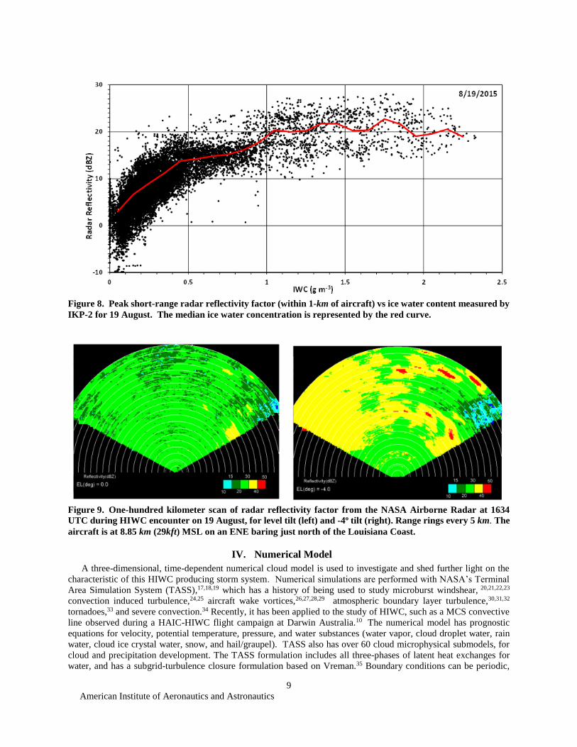
American Institute of Aeronautics and Astronautics
13
The assumed grid size is the same in all three
directions (150m) and is small enough to allow the
resolution of important thermally-driven scales of
motion
The atmospheric sounding used as input is
extrapolated from an operational weather forecast
model at a location just upstream from the system
This sounding (Fig 11) possess strong convective
instability and deep levels of moisture This sounding
also indicates a tropopause at 14km MSL with a
temperature of about -62oC or 211K Convective
indices58 computed from the sounding indicate strong
convective instability with a lifted index of about -6oC
and CAPE = 3400 J kg-1 The melting level is at
4900m MSL
The initial state of the numerical simulation is
horizontally homogeneous and varies vertically
according to the input sounding shown in Fig 11
Convection is initiated by an artificial thermal
impulse A cool pool of air that resides near the
surface over much of Louisiana and underneath the
MCS is ignored for the initial and boundary
conditions The boundary conditions for the ground
are representative of a smooth ocean surface with
constant temperature Other input parameters for the
simulation are representative of a tropical oceanic
environment (Table 5) The simulation is integrated
over a 4-hour period with convection occurring
through the full period In our simulations time (t) is in reference to time of initiation and values for the x and y
coordinates are in reference to the initial triggering impulse
B Results
The numerical simulation generates a long-lasting system with a convective line oriented in the direction of the
low-level shear vector of the environmental winds The cyclic (ie periodic) boundary conditions on the left and right
sides of the domain account for the effect of multiple lines including the interaction between the lines The type of
convection is multicellular11 with overshooting tops penetrating through the tropopause by about 600 m The system
produces persistent HIWC conditions at storm upper levels within an expanding cirrus shield fed from the multi-
Figure 11 Skew-T diagram representing initial
environmental profiles for 19 August 2015 case
Modified from sounding extracted from an operational
weather model forecast at 1400 UTC at location
upstream from the MCS (29N 912W)
Figure 10 Model Domain size relative to MCS
Table 4 Domain Size and Resolution
Domain Parameter Physical Dimension
Lateral dimensions (X Y) 45 km x 150 km
Vertical dimension (Z) 186 km
Lateral grid spacing 150 m
Vertical grid spacing 150 m
Computational grid ~39 x 10
6
grid points
Table 5 Initial Parameters
Cloud base height 625 m (942 mb)
Cloud droplet number density Ncd 75 droplets cm-3
HailGraupel particle size distribution intercept Noh
4 x 10⁵ m-4
American Institute of Aeronautics and Astronautics
14
cellular convection A comparison of the low-level radar reflectivity factor from the model simulation with the
observed NEXRAD reflectivity is shown in Fig 12
Figure 12 Comparison of low-level RRF between NEXRAD (left) and TASS (right) Observed NEXRAD
for Louisiana coast at 1645 UTC Simulated RRF at 4km altitude and 3hr 45min Outline of TASS domain
shown (90 km x 150 km)
Updrafts within the convective line generate precipitation and carry snow particles and ice crystals to the upper-
regions of the troposphere At upper levels the expanding outflow coalesces with the upper-level anvil outflow from
adjacent lines to form a large overhanging canopy (Fig 13) The general comparison between observations and
numerical simulation are summarized in
Table 6
Horizontal cross-sections at two
altitudes for RRF and IWC are shown in
Figs 14 and 15 The chosen altitudes
represent the two flight altitudes for the
DC-8 during each of two passes when
persistent IWC was measured The timing
of the slices are at a model time of
3hr45min (from the start of initialization)
and represent a time when the simulated
system has reached a mature state Profiles
are extracted along the dashed line shown
in the figures and are compared to that
measured by the DC-8 (Fig 16)
In Fig 14 the numerically simulated
ice water concentration (ice crystal snow
and graupel water combined) as well as the
RRF are shown at flight level 29 kft (8850 m) Peak ice water concentrations exceeding 3 g m-3 can be found within
small areas associated with the convective updraft turrets Larger areas with a width of about 40km exceeded 1 g m-3
Radar reflectivity factor values are generally less than 30dBZ and would appear green on the weather radar display of
most aircraft Locally higher values of RRF were found within the strong updraft cores that carry graupel and other
ice particles The RRF in Fig 14 does show large areas of low RRF but not as uniform as from the flight radar (cf
Fig 9) A more appropriate comparison would be between the RRF observed by the DC-8 with a simulation of its X-
band radar using the TASS fields as input
Figure 13 Simulated three-dimensional cloud surface viewed
from above and from south-southwest
American Institute of Aeronautics and Astronautics
15
Table 6 Comparison of general features between observed and numerically simulated for 19 August 2015 case
Feature Observed Simulated with TASS
Orientation of convective lines SSW-NNE with 45 km separation between lines
SSW-NNE with 45 km separation between lines
Cloud top elevation ~14-15 km 146 km
Coldest cloud top temperature ~200 K 203 K
Cell movement from 210o at 10 ms 221o at 11 ms
Direction of anvil canopy expansion from Southwest Southwest
Convective line movement from 290o at 6 ms 291o at 45 ms
System lifetime gt 10 hrs gt 4 hrs
Width of area with RRFgt20 dBZ at cruise altitudes
gt 50 km 40 km
At a slightly higher altitude (Fig 15) regions with HIWC cover smaller areas and have lower values of RRF This
is consistent with the measurements from the DC-8 which encountered shorter durations of IWC greater than 1
g m-3 and detected lower values of RRF after changing to a 5kft higher altitude on a subsequent pass through the
active regions near the Louisiana coast
Figure 16 shows a comparison of measured and model-extracted profiles for RRF and IWC The DC-8 flight
profiles relative to the MCS are shown in Fig 17 The TASS profiles are extrapolated at the two different altitudes
and headings flown by the DC-8 and are compared with values measured by the DC-8 At the lower elevation both
the TASS and DC-8 profiles indicate a nearly steady RRF of about 20-25 dBZ and IWC mostly between 1- 25 g m-3
At the higher elevations both TASS and DC-8 show consistent magnitudes of variation with the RRF varying between
0 to 20 dBZ and the IWC mostly remaining below 05 g m-3 Both profiles at the higher elevation do show a small
region where IWC approached 2 g m-3 Although peak values and duration of encounters seemed similar in magnitude
the variability of RRF and IWC appears greater in the modeled profiles
In Fig 18 vertical cross-sections of the simulated RRF and IWC fields are taken along the assumed flight path in
Fig 14 Note that large regions of IWC greater than 15 g m-3 (orange) extend over a large region along and below the
lower-altitude flight path Peak values occur between altitude ranges of 75-95 km AGL and drop off significantly
above 10 km AGL The corresponding RRF shows larger values below the melting level (around 5 km AGL) and very
weak values above 10 km MSL Also note that regions with significant IWC can extend above regions with low or no
detectable RRF near the ground
In summary a persistent coastal MCS system with HIWC is numerically simulated and its results compared with
data from the 2015 Florida Radar flight campaign The system is sustained by bands of convection inflowing from the
Gulf of Mexico and is capped by a large canopy cloud consisting of mostly ice crystals The simulation showed that
the coalescence of the expanding anvils from the convective cells resulted in a cloud canopy that may obscure the
banded structure and other low-level features from detection with satellite The model simulated cloud top elevations
and movement of cells appear similar to observations Largest concentrations of ice water were found in the simulation
between 75 and 95 km (25kft-31kft) MSL where environmental temperatures were between -19oC to -33oC The
range of elevations with the largest RRF were between the surface and 6km (20 kft) MSL The TASS-extracted profiles
compare reasonably with the measurements from DC-8 although some differences in variability were noted
American Institute of Aeronautics and Astronautics
16
Figure 14 Simulated RRF (left) and IWC (right) from TASS simulation at an altitude of 8850m (flight level
29kft) and 3hr and 45 min The TASS IWC field is the sum of all ice water (ice crystal water + snow + graupel)
Figure 15 Same as Fig 14 but at 10335m (flight level 34 kft)
American Institute of Aeronautics and Astronautics
17
Figure 16 Comparison of RRF and IWC extracted along flight profiles shown in Figs 14 and 15 (dashed
lines) with those measured by the DC-8 (solid lines) Top row at an altitude of 8850m bottom row at 10350m
Figure 17 Two of the DC-8 legs with longest duration of IWC
Track of DC-8 superimposed on 1645 UTC GOES-13 Infrared
satellite imagery (Courtesy NASA Langley Satellite Group)
American Institute of Aeronautics and Astronautics
18
Figure 18 Vertical cross sections of RRF (top) and IWC (bottom) extrapolated from the numerical
simulation along the flight profile shown in Fig 14 Vertical position of both flight paths shown by dashed line
Altitudes are AGL
The numerical simulation does not capture the region of stratified precipitation that lies downstream from the
inflowing convective lines However the DC-8 flights did not encounter regions of HIWC when they overflew this
region It appears likely that the rain in this area was produced by moisture from the dissipation of the convective cells
and the overrunning of the cool surface dome by the moist southerly air currents A next-generation simulation would
need to include the horizontal variation of temperature and wind into the simulation in order to capture these effects
VI Numerical Simulation of Continental Supercell Hailstorm
In this section the numerical simulation of a continental supercell hailstorm is presented The purpose of this
simulation is to validate the robustness of the microphysics used in TASS and better understand differences in HIWC
production between continental supercell storms and subtropical MCS convection Validation parameters include 1)
production of large hail 2) size of hail swath 3) radar bounded weak echo region 4) supercell features 5) storm
motion 6) size and intensity of quasi-steady updraft 7) size and maximum value of radar echo and 8) duration In
this simulation we will verify the validity of the simulation by comparing our solutions with observed data In
addition this case will be analyzed for its potential in producing HIWC and compared with the previous case of
summertime coastal convection
This case has been simulated in the past with one of the first versions of TASS using a relatively coarse mesh
Even at this earlier stage of TASS development the simulation was able to capture many of the stormrsquos observed
features5934
A Description of Observed Case
On 2 August 1981 a very large and severe hailstorm moved across Southeastern Montana The storm was observed
during its mature phase with ground-based Doppler radars and with research aircraft as it moved through a network
of field instruments during the Cooperative Convective Precipitation Experiment60 (CCOPE) The storm quickly
developed many classical features of a supercell hailstorm It veered to the right of the environmental winds and
persisted for over 5 hours while leaving a wide swath of hail The storm was reported to have an intense quasi-steady
updraft with cyclonic rotation a low-level radar hook echo signature a mid-level bounded weak echo region (BWER)
signature (same as radar echo vault) damaging winds a broad swath of 1-3 cm diameter hail with some sizes as large
American Institute of Aeronautics and Astronautics
19
as 10 cm a mesolow or mesocyclone with a peak pressure drop of at least 6mb and a peak RRF between 65-75
dBZ61626364 The primary updraft of the storm was reported to be over 14 km wide and was located within the BWER
A research aircraft flew within the updraft at an altitude between 6 km and 75 km MSL they found nearly adiabatic
conditions with updraft speeds greater than 50 m s-1 liquid water droplet concentrations of up to 6 g m-3 and the
absence of precipitation-sized particles65 The lack of larger particles explained the very low magnitudes of RRF within
the BWER Hail was penetrated by the research aircraft on the western edges of the updraft in association with the
high reflectivity regions Weisman et al66 reported that the storm produced at least one funnel cloud and that some
damage reports were ldquosuggestiverdquo of tornadic activity Surface wind speeds were estimated between 50 to 100 mph
(20 to 45 m s-1)63
A special rawinsonde sounding was launched near the storm (Fig 19) and indicated an environment very favorable
for intense convection Convective indices
calculated from the sounding exhibited a CAPE of
almost 3500 J kg-1 and a lifted Index of -10oC
The sounding also indicated a tropopause height
of 109 km MSL (~99 km AGL) with a
temperature of -475oC and an equilibrium level
at 198 mb (123 km MSL) with a temperature of -
517oC According to the both the sounding and
aircraft observations the cloud base temperature
and height were about 136oC and 26 km MSL
respectively63 The ground was slightly less than
1km above sea level and varied somewhat with
location The wind profile for the sounding
exhibited a strong magnitude of helicity6768 and
vertical shearing of the environmental wind High
values of both helicity and CAPE are indicative of
supercell and tornadic storm environments The
presence of dry environmental air at storm mid-
levels likely inhibited any strong tornado
formation (eg Proctor et al33)
B Configuration
In numerical modeling of this system we apply the
same version of the TASS model as in the Coastal-MCS
case Differences are only due to grid and domain
configuration boundary conditions input sounding and
several input parameters that define the continental
aspects of the cloud droplets and the hail size
distribution All are discussed below
The domain is size is defined to be 150 km x 150 km
in the horizontal and 20 km in the vertical (Table 7) An
evenly spaced grid size of 200 m is assumed Open
lateral boundaries conditions are applied at all lateral
boundaries The ground surface is assumed flat and no
terrain features are included The domain uses the
TASS modelrsquos internal tracking algorithms17 in
order to move the grid with the lateral translation of
the storm
The initial state profiles for temperature
pressure wind and humidity are horizontally
uniform but vary vertically according to the input
sounding shown in Fig 19 Values representative of
contental Great-Plains systems are assumed to for
the cloud droplet concentration and for the hail size
distribution intercept parameter (Table 8)
Figure 19 Skew-T diagram representing environment for
2 August 1981 Special sounding observed near Knowlton
MT at 2356 UTC Environmental wind hodograph
inserted at bottom left
Table 7 Domain Size and Resolution
Domain Parameter Physical Dimension
Lateral dimensions (X Y) 150 km x 150 km
Vertical dimension (Z) 20 km
Lateral grid spacing 200 m
Vertical grid spacing 200 m
Computational grid ~56 x 10
6
grid points
Table 8 Initial Parameters
Cloud base height (AGL) 1700 m (740 mb)
Cloud droplet number density Ncd 800 droplets cm-3
HailGraupel particle size distribution intercept Noh
2 x 10⁴ m-4
American Institute of Aeronautics and Astronautics
20
The major diffences between the initial conditions of this case and the coastal MCS case are that this case
represents a more continental environment with stronger vertical wind shear less moisture but greater instability
C Comparison of Simulation with Observations
The numerical simulation is initiated at time zero by introducing a thermal impulse and integrating over 4 hours
of time The simulation produces a supercell hailstorm and captures many of the features observed in the real storm
These include large hail wide hail swath funnel cloud with damaging surface wind 15 km wide quasi-steady updraft
surrounded at storm-mid-level by a radar echo vault or BWER a radar hook echo signature right-rear quadrant gust
front massive overshooting tops and a large spreading anvil As can be see in Table 9 scales and intenisties match
very well between the observed and simulated event The simulated updraft velocity at 65 km MSL of 55 m s-1 matches
the peak value measured by a research aircraft that penetrated the storm at the same level As found from the aircraft
measurments the updraft core was nearly adiabatic with little or no precipitation The model simulation as in the
observational studies found most of the hail to be on the western and nortwestern edges of the primary storm updraft
Table 9 Comparison of observations with TASS for 2 August 1981 Supercell Hailstorm
Features Observed TASS Simulated Anvil Extent Downstream from Updraft
(based on Radar Echo) gt200 km gt150 km
Anvil Extent Upstream from Updraft gt20 km gt60 km
BWER Diameter ~75 km ~8 km
BWER Vertical Extent 10 75 km MSL 12-14 km MSL
Gust Front Location SW Flank SW Flank
Peak Gust Front Wind Speed gt20 ms 25 ms
Typical Hail Diameter at Surface 1-3 cm peak median diameter 2 cm
Hail Shaft Location Relative to Center of BWER 3-4 km West 4-6 km WNW
Width of Hail Swath 20-30 km 225 km
Supercell Lifetime gt 5 hrs gt 4 hrs
Persistent Low-Level Radar Hook Echo yes Yes
Maximum Liquid Cloud Water Content 65 g m-3 55 g m-3
Surface Pressure Drop 6 mb Mesocyclone 4 mb tornado 21 mb
Peak Rainfall Accumulation 30-35 mm 25 mm
Peak Radar Reflectivity Factor 75 dBZ 726 dBZ
Storm Movement (development stage) 260 at 10 ms 250 at 12 ms
Storm Movement (supercell stage) 282 at 18 ms 280 at 16 ms
Storm Top Overshoot above EL 3-4 km 5 km
Updraft Diameter 14-17 km 15 km
Max Updraft Velocity at 65 km MSL 53 ms 55 ms
Diameter of 20 dBZ Echo at 12 km MSL 45 km 45 km
Peak Surface-Level Gusts East of Updraft gt25 ms 30 ms
Radar Echo Top 16 km MSL 18 km MSL
Tornadoes Funnel cloud sighted Yes western side of mesocyclone
Peak Surface Wind Damage F1- wind damage (estimated 33-50 ms)
56 ms
Maximum Altitude of 10 dbZ Contour in BWER 6-8 km MSL 65 km MSL
American Institute of Aeronautics and Astronautics
21
Supercell environments often produce tornadoes or familes of tornadoes and a funnel cloud with surface wind
damage was reported with this system The funnel cloud that was produced in the numerical simulation was
intermittent and dissiapted when it moved into the cooler dryer air underneath the hail and rain shafts Tornado
formation in this simulation showed similar characteristics to those studied in an earlier paper where the presence of
dry mid-level air acts to weaken or suppress tornado formaition in supercell environments33
The time evolution of the area with RRF greater than 55 dBZ at an elevation of 5 km MSL (blue) and the peak
RRF anywhere in the storm (red) is shown in Fig 20 The peak RRF from the simulation matches the observations
very well For the area with RRF greater than 55 dBZ both observation and TASS show a ramp up in the first two
hours of the stormrsquos lifetime but the
simulation shows this area to be smaller
than detected by ground-based radar
A comparison of the supercell structure
from TASS with measurements from
ground-based radar are shown in Figs 21
and 22 Two horizontal levels of RRF are
shown one at 10 km MSL and the other at 4
km MSL The TASS simulation reproduces
many of the observed features and supercell
signatures including the BWER (ie radar
echo Vault (V)) the radar hook echo and
the radar echo streamer The scale of the
area covered by each intensity of RRF are
similar between TASS and observed as
well One contrast however is that the high-
reflectivity area within the hook echo region
appears larger in the observation than in the
simulation The area of highest reflectivity
which is west and northwest of the BWER
is associated with large hail in both
observation and simulation
In Fig 23 a vertical cross-section along
x-z coordinates is taken through the middle
of the BWER Again both the simulation and observation show similar features similar intensities and similar spatial
scales The BWER or radar Vault is clearly present in the simulation and extends deep into the storm The BWER
is located within the intense storm updraft and is produced by a lack of significant precipitation-sized particles
D HIWC Characteristics in Simulated Storm
The Montana supercell with its quasi-steady large diameter and intense updraft generates large volumes of ice
crystals that are transported into the upper regions of the troposphere Increasing wind speeds with height which is a
characteristic of supercell environments quickly transports many of the ice particles downstream within a large
expanding anvil cloud Hail and larger ice particles are also carried up to high altitudes by the strong updrafts but fall
out relatively close-by due to their significant fall velocities Therefore large values of RRF can be found at storm
upper-levels within proximity to the supercell updraft The RRF drops-off with distance from the updraft as the larger
particles fall out and the remaining smaller particles are carried downstream
A graphical representation of the cloud and precipitation fields from TASS is show in Fig 24 Overshooting tops
which are above the predominant supercell updraft can penetrate several kilometers into the stratosphere A large
anvil cloud spreads mostly downstream from the overshooting tops due to the strong westerly winds beneath the
tropopause (cf Fig 9) This anvil cloud covers many square kilometers and forms a large overhang of cloud material
downstream from the storm updraft Due to the intensity of the updraft some the anvil material is transported counter
to upper-level winds and produces a forward overhang upstream from the storm updraft
The coldest cloud tops (Fig 25) are associated with the overshooting tops above the intense storm updraft Cloud
tops at temperaturesheights near the equilibrium level expand over a large area downstream from the overshooting
tops Obviously in Fig25 the anvil expands northeastward beyond the boundaries of the model domain
Figure 20 Time evolution of the maximum RRF anywhere
in the storm (red) and the cross-sectional area of reflectivity
exceeding 55 dBZ at 5km MSL (blue) Observed values from
Miller et al63(solid) compared with TASS (dashed)
American Institute of Aeronautics and Astronautics
22
Figure 22 Same as Fig 21 but RRF at an elevation of 4 km MSL Left adapted
from Millerrsquos analysis of ground based Doppler radar right from TASS at
t=3hr07min
RRF (dBZ)
Figure 21 Horizontal cross-section of Radar reflectivity factor at an altitude of
10 km MSL Left adapted from Millerrsquos analysis of ground based Doppler radar62
right from TASS at t=3hr07min Both plots windowed to 50km x 50km area with
major tick every 10 km The Radar echo Vault or BWER identified with V
Figure 23 Same as Fig 21 but RRF along vertical west-east cross-section through
BWER Left adapted from Millerrsquos analysis of ground based Doppler radar right from
TASS at t=3hr07min Altitude in km AGL with major ticks every 1km along abscissa
American Institute of Aeronautics and Astronautics
23
Very similar features for the simulated Montana supercell storm can be seen in the observed visible satellite
imagery of the actual system (Fig 26) The overshooting tops are positioned near the southern end and the anvil
expands toward the north-northeast The horizontal dimension of the observed cloud anvil compared with the cloud
top depicted in Fig 25 are nearly identical
Figure 27 shows the simulated IWC and RRF along a horizontal cross-section taken at 10km MSL (9km AGL)
The size and shape of the system represented in the cross-section is consistent with the satellite imagery in Fig 26 In
Fig 27 most of the RRF greater than 20 dBZ is confined to area within a 50 km diameter centered about the primary
updraft and BWER Values of RRF between 15-20 dBZ cover large areas downstream for the overshooting tops
Figure 27 also shows vast areas with IWC greater than 1 g m-3 In fact areas with 1 g m-3 or greater can be found at
distances of up to 50 to 100 km away from the regions with the greatest storm RRF Our simulation seems to imply
that by avoiding the high reflectivity areas by 20 nautical miles (37 km) may not be sufficient for avoiding prolonged
HIWC exposures
Figure 24 Simulated cloud and precipitation surfaces within the full TASS domain Viewed from south
Figure 25 Cloud top temperatures from TASS at 3hr75 min (left) and 3hr45min (right) simulation
time Coldest temperatures associated with overshooting tops in southwestern quadrant of figure
American Institute of Aeronautics and Astronautics
24
To further explore the structure of the simulated storm
vertical cross-sections are extracted alone lines A-B and C-D
that that appear in Fig27 These cross sections are shown in
Figs 28 and 29 They also help illustrate where HIWC
conditions may be found relative to the storm
The cross-sections through A-B (Fig 28) are taken
northeastward through the storm updraft It shows strong
reflectivity surrounding the BWER and extending to the upper
levels of the storm High levels of IWC largely composed of
hail are brought to the ground on the southwestern side of the
storm updraft and at upper-levels surrounding the updraft
Aircraft routinely avoid these areas due to their high values of
RRF More of a factor to air traffic is that significant levels of
IWC that can be found over large areas within the cloud
canopy at great distances downstream from the stormrsquos high
reflectivity regions Furthermore the RRF within the canopy
are very low and could be undetectable with many airborne
weather radars
In Fig 29 a cross section is taken orthogonal to the
direction of the shearing anvil It is taken northwestward
between C and D along the edge of the areas with significant
IWC (Fig 27) This cross-section resides at least 70 km or
more from areas with high RRF Along this cross section IWC
greater 1 g m-3 can be seen to extend for over a 100 km length
The layer has a thickness that is several kilometers thick This
layer also consist of very weak RRF (lt 20 dBZ) and
underneath has no detectable radar reflectivity or precipitation
Both cross-sections show that a layer with HIWC can extend over large distances and with very weak RRF
Beneath this layer containing HIWC precipitation was rarely apparent and radar reflectivity not detectable One visual
queue sometimes recommended to pilots for helping to identify potential HIWC conditions is the presence of strong
to moderate RRF from rain beneath regions of HIWC This queue would not apply to a supercell storm such as this
This case of a continental supercell also demonstrates that HIWC risks may not be confined to just oceanic and
coastal MCS since regions of significant IWC may extend for large distances with little RRF
VII Discussion and Conclusion
Flight data and results from numerical simulations are analyzed to better characterize the HIWC threat for aircraft
and to improve our understanding of the relationship between HIWC radar and satellite signatures Flight
measurements with airborne radar and microphysical probes suggest that RRF alone may not be adequate for the
detection of HIWC conditions This fact also is reinforced from the numerical model simulations
The numerical simulations confirm that HIWC can be produced in contrasting environments In warm moist
coastal and oceanic environments large volumes of ice crystals can be pumped into the upper-troposphere by
regenerating convective plumes associated with a long-lasting system Cloud material carried in the upper-level
outflow from these plumes coalesces to form a large overhanging canopy and contain significant concentrations of
ice crystals Perhaps due to the weaker wind shear of these environments and the duration of the systems large
concentrations may accumulate over time
Our simulation of a large continental supercell shows it to have a large persistent and nearly adiabatic updraft
that also can pump large volumes of ice crystals in to the upper troposphere Vertical windshear with strong winds
aloft (which are an ingredient in producing supercells) can act to transport ice crystals over large areas We speculate
that the increase ventilation due to environmental wind shear may dilute the peak concentrations of IWC in supercells
Figure 26 Observed visible satellite imagery
from GOES-7 Northeastern Montana 2315
UTC 2 August 1981
American Institute of Aeronautics and Astronautics
25
Figure 27 Ice water content (left) and RRF (right) from TASS at an elevation of 10km MSL and 3hr45
min) simulation time Ice water content (g m-3) is sum of ice crystal snow and hail water content Units
for RRF are (dBZ)
Figure 28 Vertical cross section along A-B in Fig 27 Top is ice water content (g m-3) and bottom is RRF
(dBZ) Altitudes are above ground level
American Institute of Aeronautics and Astronautics
26
In our study the microphysics for snow is improved by using analyzed PSD data measured during the flight
campaign A new relationship is developed that relates the exponential size-distribution intercept for ice particles with
their water content In the past the value for the intercept has been assumed constant or a function of temperature
only The new relationship is a function of snow or ice water content as well as temperature and was used to improve
the microphysical submodels in TASS
The TASS model was then applied to contrasting types of convection and compared to available observations
This comparison seemed very good and demonstrated the model could be applied robustly to convection in different
types of environments Excellent results were achieved using only simple bulk parametrizations for microphysics
suggesting that models that are more complex may not be needed depending upon application The profiles of ice
water content and RRF extracted from the simulation compared reasonably well with the measurements by the DC-8
during penetrations of the coastal MCS although some differences in variability were noted The TASS model was
also used to simulate a specific supercell hailstorm with excellent comparison to measurements in terms structure
features scales and magnitudes
The numerical studies for both cases found that regions of significant IWC could extend above regions with little
or no RRF This would imply that moderate to high radar reflectivity might not always be underneath HIWC events
Yet to be investigated is the potential for HIWC detection using a combination of sensors and sources for
information (ie satellite and other weather data) Also unexplored is the ability to detect HIWC with advanced
airborne radar tools
Appendix Ice Crystal Size Distributions
Relationships between the ice crystal size distributions temperature and ice water content are needed for the
parameterization of microphysical submodels used in TASS These relationships could be useful in other applications
such as the understanding the radar reflectivity factor (RRF) due to ice crystals Dr Alexei Korolev processed the
particle size distribution (PSD) data69 from data collected at one-Hertz intervals during the DC-8 flights from a 2D-S
probe and a particle-imaging probe (PIP) The measured data was discretized into appropriate size bins and normalized
by the width of the corresponding bin This allowed for the direct comparison of the PSD data with different size
resolutions and common theoretical drop-size distributions (eg Marshall-Palmer70) The size resolution for the 2D-S
probe was10 μm and 100 μm for the PIP The range of particle measurements extends from 15 μm to 12845 mm The
Figure 29 Same as in Fig 28 but for position C-D in Fig 27
American Institute of Aeronautics and Astronautics
27
size of irregularly shaped ice particles as estimated from particle images may be defined in several different ways
The composite PSD data used the length of the particle parallel to the photodiode array commonly called Ly
An intercept (N0) and slope (λ) parameter were found from the data by using a least-squares method to fit an
exponential distribution through the measured PSD This was repeated for all times in a flight Relationships can then
be established for N0S vs ice water content (IWC) and atmospheric temperature
Our numerical modeling effort previously employed a relationship for Nos that is a function of temperature
only1017 Recall that our snow category represents the larger ice particles (excluding graupel and hail) and assumes
an inverse exponential size distribution whereas our cloud ice category only represents the smaller ice particles with
diameters less than about 200 um Using combined data measured from each day of the NASA deployment (Table 1)
and binning according to temperature a new relationship was determined for Nos that is a function of both temperature
and snow water content Ms
Log10 (Nos) = 744 ndash 00217 Tc +10526 Ms ndash 015 Ms2 +0004 Ms3 (A-1)
for Tcgt -55OC and Ms lt 4 g m-3
where Nos has units of m-4 Ms has units of g m-3 and Tc is temperature of the environment in centigrade The
relationship was fitted from the flight data as shown in Fig A1 and produces a larger intercept value for either colder
temperatures or increasing snow water content A higher intercept value translates into a distribution with overall
smaller particles lower radar reflectivity factor and slightly slower fall velocity Other parameterized microphysical
processes are affected by the assumption for Nos these include sublimation or deposition of snow particles and other
growth processes
Note that when Ms 0 the above relationship asymptotes to a relationship suggested by Woods et al71 who
derived their relationship from analyzing ice particles in wintertime precipitation occurring in the Pacific Northwest
Based on all ice particles they found the following relationship for No
Log10 (No ) = 753 ndash 00207 Tc (A-2)
Since their measured ice water contents ranged between 003 and 030 g m-3 it would have been difficult for them to
detect any dependency of No on ice water content
As a further check to the validity Eq (A-1) we compare the observed short-range RRF with the value estimated
from the measured IWC using the assumption of an inverse exponential size distribution with Eq (1) as
ZS [mm6m3] = 390 x 108 Ms175 Nos
-075 (A-3)
where the above assumes melted spherical particles and accounts for the differences in radar dielectric constants for
ice and water
The comparisons are shown in Fig A1 and illustrates the lack of correlation of radar reflectivity with snow water
concentration for values of snow water greater than about 1 g m-3
American Institute of Aeronautics and Astronautics
28
Figure A1 Ice particle distribution intercept NoS
vs ice water content for three temperature ranges
Data points derived from PSD distributions
measured during all 2015 DC-8 Flight Campaign
flights (ie Table 1) Blue curve represents medium
value Red curve is fit using Eq (A-1)
Figure A2 Radar reflectivity factor vs ice
water content for three temperature ranges
Data points of close-range RRF measured during
all 2015 DC-8 Flight Campaign flights (ie Table
1) Blue curve represents medium value Red
curve using Eqs (A-3) and (A-1)
American Institute of Aeronautics and Astronautics
29
Acknowledgments
This research is sponsored by the Advanced Air Transport Technology Project of NASArsquos Advanced Air Vehicles
Program The authors would like to acknowledge the contributing organizations that enabled the Florida HIWC Radar
Flight Campaign the FAA Aviation Research Division and Aviation Weather Division the NASA Aviation Safety
Program the Boeing Company Met Analytics Science Engineering Associates Environment Canada the National
Center for Atmospheric Research Honeywell and Rockwell Collins The authors also would like to thank Tom
Ratvasky (NASA Glenn Research Center) and Walter Strapp (Met Analytics) for their programmatic technical and
operational support and the NASA Langley Satellite Group for providing satellite images In addition thanks to
Alexei Korolev (Environment and Climate Change Canada) for processing the PSD data from raw data collected
during the flight test The numerical simulations were conducted using the Pleiades high-performance supercomputer
cluster of the NASA Advanced Supercomputing Division
References
1Mason JG Strapp JW and Chow P ldquoThe Ice Particle Threat to Engines in Flightrdquo AIAA 2006-206 doi10251462006-
206 2Mason JG and Grzych M ldquoThe Challenges Identifying Weather Associated with Jet Engine Ice Crystal Icingrdquo SAE
International 2011-38-0094 doi1042712011-38-0094 3Bravin M Strapp JW and Mason J ldquoAn Investigation into Location and Convective Lifecycle Trends in an Ice Crystal
Icing Engine Event Databaserdquo SAE International 2015-01-2130 doi1042712015-01-2130 4Addy HE Jr and Veres JP ldquoAn Overview of NASA Engine Ice-Crystal Icingrdquo SAE International 2011-38-0017
doi1042712011-38-0017 5Grandin A Merle J-M Weber M Strapp JW Protat A and King P ldquoAIRBUS Flight Tests in High Ice Water Content
Regionsrdquo AIAA 2014-2753 doi10251462014-2753 6Protat A and Rauniyar S Kumar VV and Strapp JW ldquoOptimizing the Probability of Flying in High Ice Water Content
Conditions in the Tropics Using a Regional-Scale Climatology of Convective Cell Propertiesrdquo Journal of Applied Meteorology
and Climatology Vol 53 November 2014 pp 2438-2456 doi101175jamc-d-14-00021 7Dezitter F Grandin A Brenguier JL Hervy F Schlager H Villedieu P and Zalamansky G ldquoHAIC (High Altitude
Ice Crystals)rdquo AIAA 2013-2674 doi10251462013-2674 8Houze RA Jr ldquoMesoscale Convective Systemsrdquo Review of Geophysics Vol 42 RG4003 2004 pp 1-43
doi1010292004RG000150 9Grzych M Tritz T Mason J Bravin M and Sharpsten A ldquoStudies of Cloud Characteristics Related to Jet Engine Ice
Crystal Icing Utilizing Infrared Satellite Imagerrdquo SAE International 2015-01-2086 doi1042712015-01-2086 10Proctor FH and Switzer GF ldquoNumerical Simulation of HIWC Conditions with the Terminal Area Simulation Systemrdquo
AIAA-2016-4203 doi10251462016-4203 11Houze RA Jr Cloud Dynamics Ed Academic Press 1993 573 pp doi101002qj49712051918 12FAA ldquoTurbojet Turboprop and Turbofan Engine Induction System Icing and Ice Ingestionrdquo February 2004 Advisory
Circular 20-147 doi104271510198 13Davison CR Strapp JW Lilie L Ratvasky TP Dumont C ldquoIsokinetic TWC Evaporator Probe Calculations and
Systemic Uncertainty Analysisrdquo AIAA 2016-4060 doi10251462016-4060 14Strapp JW Lilie LE Ratvasky TP Davison C and Dumont C ldquoIsokinetic TWC Evaporator Probe Development of
the IKP2 and Performance Testing for the HAIC-HIWC Darwin 2014 and Cayenne-2015 Field Campaignsrdquo AIAA 2016-4059
doi10251462016-4059 15Lilie LE Sivo CP and Bouley DB ldquoDescription and Results for a Simple Ice Crystal Detection System for Airborne
Applicationsrdquo AIAA 2016-4058 doi10251462016-4058 16Crum TD and Alberty RL ldquoThe WSR-88D and the WSR-88D Operational Support Facilityrdquo Bulletin of the American
Meteorological Society Vol 74 No 9 1993 pp 1669-1688 doi1011751520-0477
doi1011751520-0477(1993)074lt1669TWATWOgt20CO2 17Proctor FH ldquoThe Terminal Area Simulation System Volume I Theoretical Formulationrdquo April 1987 NASA CR-4046 18Proctor FH ldquoNumerical Simulation of Wake Vortices Measured During the Idaho Falls and Memphis Field Programsrdquo
14th AIAA Applied Aerodynamic Conference Proceedings Part II June 1996 AIAA 96-2496-CP pp 943-960
doi10251461996-2496 19Proctor FH ldquoInteraction of Aircraft Wakes from Laterally Spaced Aircraftrdquo AIAA 2009-0343 doi10251462009-343 20Proctor FH ldquoNumerical Simulations of an Isolated Microburst Part I Dynamics and Structurerdquo Journal of the
Atmospheric Sciences Vol 45 pp 3137-3160 doi1011751520-0469(1988)045lt3137nsoaimgt20co2 21Proctor FH and Bowles RL ldquoThree-Dimensional Simulation of the Denver 11 July 1988 Microburst-Producing Stormrdquo
Meteorology and Atmospheric Physics Vol 49 1992 pp 107-124 doi101007bf01025403 22Proctor FH 1989 ldquoNumerical Simulations of an Isolated Microburst Part II Sensitivity Experimentsrdquo Journal of the
Atmospheric Sciences Vol 46 15 July 1989 pp 2143-2165 doi1011751520-0469(1989)046lt2143nsoaimgt20co2
American Institute of Aeronautics and Astronautics
30
23Proctor FH Bracalente EM Harrah SD Switzer GF and Britt CL ldquoSimulation of the 1994 Charlotte Microburst
with Look-Ahead Windshear Radarrdquo Preprints 27th Conference on Radar Meteorology American Meteorological Society October
1995 pp 530-532 Paper-10B-7 24Proctor FH Hamilton DW and Bowles RL ldquoNumerical Study of a Convective Turbulence Encounterrdquo AIAA 2002-
0944 doi10251462002-944 25Ahmad NN and Proctor FH ldquoLarge Eddy Simulations of Severe Convection Induced Turbulencerdquo AIAA 2011-3201
doi10251462011-3201 26Han J Lin Y-L Schowalter DG Arya SP and Proctor FH ldquoLarge Eddy Simulation of Aircraft Wake Vortices within
Homogeneous Turbulence Crow Instabilityrdquo AIAA Journal Vol 38 February 2000 pp 292-300 doi1025142956 27Proctor F 2004 report H Hamilton DW and Han J ldquoWake Vortex Transport and Decay in Ground Effect Vortex
Linking with the Groundrdquo AIAA 2000-0757 doi10251462000-757 28Proctor FH Hamilton DW Rutishauser DK and Switzer GF ldquoMeteorology and Wake Vortex Influence on American
Airlines FL-587 Accidentrdquo April 2004 NASA TM-2004-213018 29Proctor FH ldquoNumerical Study of a Long-Lived Isolated Wake Vortex in Ground Effectrdquo AIAA 2014-2469
doi10251462014-2469 30Schowalter DG DeCroix DS Lin Y-L Arya SP and Kaplan ML ldquoPlanetary Boundary Layer Simulation using
TASSrdquo April 1996 NASA CR-198325 31DeCroix DS Lin Y-L and Schowalter DG ldquoCellular Convection Embedded in the Convective Planetary Boundary
Layerrdquo Journal of Wind Engineering and Industrial Aerodynamics Vol 67 pp 387-401 doi101016s0167-6105(97)00088-3 32Ding F Arya SP Lin Y-L ldquoLarge-Eddy Simulation of the Atmospheric Boundary Layer Using a New Subgrid-Scale
Model II Weakly and Moderately Stable Casesrdquo Environmental Fluid Mechanics Vol 1 2001 pp 49-69
doi101023a1011543715591 33Proctor FH Ahmad NN and Limon Duparcmeur FM ldquoNumerical Simulation of a Tornado Generating Supercellrdquo
AIAA 3012-0557 doi10251462012-557 34Proctor FH ldquoThe Terminal Area Simulation System Volume II Verification Experimentsrdquo April 1987 NASA CR- 4047 35Vreman AW ldquoAn Eddy-Viscosity Subgrid-Scale Model for Turbulent Shear Flow Algebraic Theory and Applicationsrdquo
Physics of Fluids Vol 16 October 2004 pp 3670-3681 doi10106311785131 36Proctor FH and Han J ldquoNumerical Study of Wake Vortex Interaction with Ground Using the Terminal Area Simulation
Systemrdquo AIAA 99-0754 doi10251461999-754 37Switzer G and Proctor F ldquoTerminal Area Simulation System Userrsquos Guide ndash Version 100rdquo January 2014 NASA TM-
2014-218150 38Proctor FH ldquoNumerical Simulation of Wake Vortices Measured During the Idaho Falls and Memphis Field Programsrdquo
14th AIAA Applied Aerodynamic Conference Proceedings Part II June 1996 AIAA 96-2496-CP pp 943-960
doi10251461996-2496 39Leonard BP MacVean MK and Lock AP ldquoThe Flux-Integral Method for Multidimensional Convection and Diffusionrdquo
Applied Mathematical Modeling Vol 19 1995 pp 333-342 doi1010160307-904x(95)00017-e 40van Leer B ldquoTowards the Ultimate Conservative Difference Scheme V A Second-Order Sequel to Godunovrsquos Methodrdquo
Journal of Computational Physics Vol 32 1979 pp 101-136 doi1010160021-9991(79)90145-1 41Ahmad NN and Proctor FH ldquoAdvection of Microphysical Scalars in Terminal Area Simulation System (TASS)rdquo AIAA
2011-1004 doi10251462011-1004 42Klemp JB and Wilhelmson R ldquoThe Simulation of Three-Dimensional Convective Storm Dynamicsrdquo Journal of the
Atmospheric Sciences Vol 35 June 1978 pp 1070-1096 doi1011751520-0469(1978)035lt1070tsotdcgt20co2 43Wang CY ldquoExact Solutions of the Navier-Stokes Equations ndash The Generalized Beltrami Flows Review and Extensionrdquo
Acta Mechanica Vol 81 1990 pp 69-74 doi101007bf01174556 44Switzer GF ldquoValidation Tests of TASS for Application to 3-D Vortex Simulationsrdquo October 1996 NASA CR-4756 45Bull JR and Jameson A ldquoSimulation of the Compressible Taylor Green Vortex using High-Order Flux Reconstruction
Schemesrdquo AIAA 2014-3210 doi10251462014-3210 46Chapelier J-B Plata MDLL and Renac F ldquoInviscid and Viscous Simulations of the Taylor-Green Vortex Using a Modal
Discontinuous Galerkin Approachrdquo AIAA 2012-3073 doi10251462012-3073 47DeBonis JR ldquoSolutions of the Taylor-Green Vortex Problem Using High-Resolution Explicit Finite Difference Methodsrdquo
AIAA 2013-0382 doi10251462013-382 48Ahmad N and Proctor FH ldquoSimulation of Benchmark Cases with the Terminal Area Simulation Systemrdquo AIAA 2011-
1005 doi10251462011-1005 49Lin Y-L Farley RD and Orville HD ldquoBulk Parameterizations of the Snow Field in a Cloud Modelrdquo Journal of Climate
and Applied Meteorology Vol 32 1983 pp 1065-1092 doi1011751520-0450(1983)022lt1065bpotsfgt20co2 50Rutledge SA and Hobbs PV ldquoThe Mesoscale and Microscale Structure and Organization of Clouds and Precipitation
VIII A Model for the ldquoSeeder-Feederrdquo Process in Frontal Rainbandsrdquo Journal of the Atmospheric Sciences Vol 40 May 1983
pp 1185-1206 doi1011751520-0469(1983)040lt1185tmamsagt20co2
American Institute of Aeronautics and Astronautics
31
51Berry EX and Reinhardt RE ldquoAn Analysis of Cloud Drop Growth by Collection Part I Double Distributionsrdquo Journal
of the Atmospheric Sciences Vol 31 October 1974 pp 1814-1824 doi1011751520-0469(1974)031lt1814aaocdggt20co2 52Berry EX and Reinhardt RE ldquoAn Analysis of Cloud Drop Growth by Collection Part II Single Initial Distributionsrdquo
Journal of the Atmospheric Sciences Vol 31 October 1974 pp 1825-1831
doi1011751520-0469(1974)031lt1825aaocdggt20co2 53Proctor FH 1989 ldquoNumerical Simulations of an Isolated Microburst Part II Sensitivity Experimentsrdquo Journal of the
Atmospheric Sciences Vol 46 15 July 1989 pp 2143-2165 doi1011751520-0469(1989)046lt2143nsoaimgt20co2 54Sekhon RS and Srivastava RC ldquoDoppler Radar Observations of Drop-Size Distributions in a Thunderstormrdquo Journal of
the Atmospheric Sciences Vol 28 September 1971 pp 983-994 doi1011751520-0469(1971)028lt0983droodsgt20co2 55Musil DJ ldquoComputer Modeling of Hailstone Growth in Feeder Cloudsrdquo Journal of the Atmospheric Sciences Vol 27
1970 pp474-482 doi1011751520-0469(1970)027lt0474cmohgigt20co2 56Smith PL Jr Myers CG and Orville HD ldquoRadar Reflectivity Factor Calculations in Numerical Cloud Models using
Bulk Parameterizations of Precipitationrdquo Journal of Applied Meteorology Vol 14 September 1975 pp 1156-1165
doi1011751520-0450(1975)0143C1156rrfcin3E20co2 57Rogers RR A Short Course in Cloud Physics Pergamon Press 1976 227 pp doi101007bf00876948 58Blanchard DO ldquoAssessing the Vertical Distribution of Convective Available Potential Energyrdquo Weather and Forecasting
Vol 13 No 3 September 1998 pp 870-877 doi1011751520-0434(1998)013lt0870atvdocgt20co2 59Proctor FH 1985 ldquoThree Dimensional Simulation of the 2 August CCOPE Hailstorm with the Terminal Areas Simulation
Systemrdquo Report of the International Cloud Modelling WorkshopConference World Meteorological Organization WMP Report
No8 Technical Document WMOTD-139 September 1986 pp 227-240 60Knight CA ldquoThe Cooperative Convective Precipitation Experiment (CCOPE) 18 May -7 August 1981rdquo Bulletin of the
American Meteorological Society Vol 63 No 4 April 1982 pp 386-398
doi1011751520-0477(1982)063lt0386tccpemgt20co2 61Wade CG ldquoA Preliminary Study of an Intense Thunderstorm Which Moved Across the CCCOPE Research Network in
Southeastern Montanardquo Preprints 9th Conference on Forecasting and Analysisrdquo American Meteorological Society 1982 pp 388-
395 62Miller LJ ldquoThe CCOPE Hailstorm of 2 August 1981rdquo Report of the International Cloud Modelling WorkshopConference
World Meteorological Organization WMP Report No8 Technical Document WMOTD-139 September 1986 pp193-198 63Miller LJ Tuttle JD and Knight CA ldquoAirflow and Hail Growth in a Severe Northern High Plains Supercell ldquo Journal
of the Atmospheric Sciences Vol 45 No 4 1988 pp 736 doi1011751520-0469(1988)045lt0736aahgiagt20co2 64Wang PK ldquoMoisture Plumes Above Thunderstorm Anvils and their Contributions to Cross-Tropopause Transport of Water
Vapor in Midlatitudesrsquo Journal of Geophysical Research Vol 108 No D6 4194 2003 doi1010292002jd002581 65Musil DJ Heymsfield AJ and Smith PL ldquoMicrophysical Characteristics of a Well-Developed Weak Echo Region in a
High Plains Supercell Thunderstormrdquo Journal of Climate and Applied Meteorology Vol 25 July 1986 pp 1037-1051
doi1011751520-0450(1986)025lt1037mcoawdgt20co2 66Weisman ML Klemp J Miller LJ ldquoModeling and Doppler Analysis of the CCOPE August 2 Supercell Storm Preprints
13th Conference on Severe Local Storms American Meteorology Society 1983 pp 223226 67Davies-Jones RP Burgess D and Foster M ldquoTest of Helicity as a Tornado Forecast Parameterrdquo Preprints 16th Conf
on Severe Local Storms American Meteorological Society 1990 pp 588ndash592 68Brooks HE Doswell CA III and Cooper J ldquoOn the Environments of Tornadic and Nontornadic Mesocyclonesrdquo
Weather Forecasting Vol 9 December 1994 pp 606-618 doi1011751520-0434(1994)009lt0606oteotagt20co2 69Korolev A and Sussman B ldquoA Technique for Habit Classification of Cloud Particlesrdquo Journal of Atmospheric and
Oceanic Technology Vol 17 August 2000 pp 1048-1057 doi1011751520-0426(2000)017lt1048atfhcogt20co2 70Marshall JS and Palmer WM ldquoThe Distribution of Rain-Drops with Sizerdquo Journal of the Atmospheric Sciences Vol 5
1948 pp 179-207 doi1011751520-0469(1948)005lt0165tdorwsgt20co2 71Woods CP Stoelinga MT and Locatelli JD ldquoSize Spectra of Snow Particles Measured in Wintertime Precipitation in
the Pacific Northwestrdquo Journal of the Atmospheric Sciences Vol 65 January 2008 pp 189- 205 doi1011752007jas22431
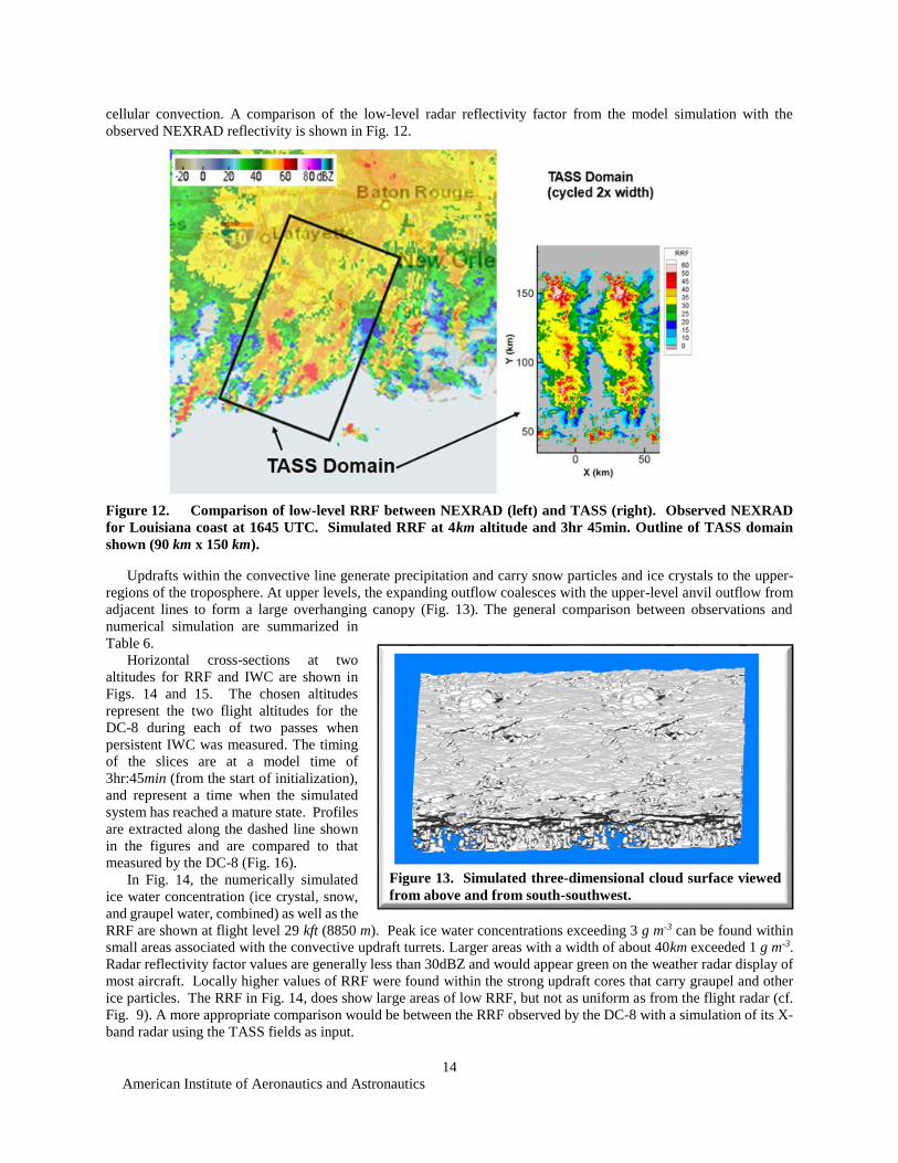
American Institute of Aeronautics and Astronautics
15
Table 6 Comparison of general features between observed and numerically simulated for 19 August 2015 case
Feature Observed Simulated with TASS
Orientation of convective lines SSW-NNE with 45 km separation between lines
SSW-NNE with 45 km separation between lines
Cloud top elevation ~14-15 km 146 km
Coldest cloud top temperature ~200 K 203 K
Cell movement from 210o at 10 ms 221o at 11 ms
Direction of anvil canopy expansion from Southwest Southwest
Convective line movement from 290o at 6 ms 291o at 45 ms
System lifetime gt 10 hrs gt 4 hrs
Width of area with RRFgt20 dBZ at cruise altitudes
gt 50 km 40 km
At a slightly higher altitude (Fig 15) regions with HIWC cover smaller areas and have lower values of RRF This
is consistent with the measurements from the DC-8 which encountered shorter durations of IWC greater than 1
g m-3 and detected lower values of RRF after changing to a 5kft higher altitude on a subsequent pass through the
active regions near the Louisiana coast
Figure 16 shows a comparison of measured and model-extracted profiles for RRF and IWC The DC-8 flight
profiles relative to the MCS are shown in Fig 17 The TASS profiles are extrapolated at the two different altitudes
and headings flown by the DC-8 and are compared with values measured by the DC-8 At the lower elevation both
the TASS and DC-8 profiles indicate a nearly steady RRF of about 20-25 dBZ and IWC mostly between 1- 25 g m-3
At the higher elevations both TASS and DC-8 show consistent magnitudes of variation with the RRF varying between
0 to 20 dBZ and the IWC mostly remaining below 05 g m-3 Both profiles at the higher elevation do show a small
region where IWC approached 2 g m-3 Although peak values and duration of encounters seemed similar in magnitude
the variability of RRF and IWC appears greater in the modeled profiles
In Fig 18 vertical cross-sections of the simulated RRF and IWC fields are taken along the assumed flight path in
Fig 14 Note that large regions of IWC greater than 15 g m-3 (orange) extend over a large region along and below the
lower-altitude flight path Peak values occur between altitude ranges of 75-95 km AGL and drop off significantly
above 10 km AGL The corresponding RRF shows larger values below the melting level (around 5 km AGL) and very
weak values above 10 km MSL Also note that regions with significant IWC can extend above regions with low or no
detectable RRF near the ground
In summary a persistent coastal MCS system with HIWC is numerically simulated and its results compared with
data from the 2015 Florida Radar flight campaign The system is sustained by bands of convection inflowing from the
Gulf of Mexico and is capped by a large canopy cloud consisting of mostly ice crystals The simulation showed that
the coalescence of the expanding anvils from the convective cells resulted in a cloud canopy that may obscure the
banded structure and other low-level features from detection with satellite The model simulated cloud top elevations
and movement of cells appear similar to observations Largest concentrations of ice water were found in the simulation
between 75 and 95 km (25kft-31kft) MSL where environmental temperatures were between -19oC to -33oC The
range of elevations with the largest RRF were between the surface and 6km (20 kft) MSL The TASS-extracted profiles
compare reasonably with the measurements from DC-8 although some differences in variability were noted
American Institute of Aeronautics and Astronautics
16
Figure 14 Simulated RRF (left) and IWC (right) from TASS simulation at an altitude of 8850m (flight level
29kft) and 3hr and 45 min The TASS IWC field is the sum of all ice water (ice crystal water + snow + graupel)
Figure 15 Same as Fig 14 but at 10335m (flight level 34 kft)
American Institute of Aeronautics and Astronautics
17
Figure 16 Comparison of RRF and IWC extracted along flight profiles shown in Figs 14 and 15 (dashed
lines) with those measured by the DC-8 (solid lines) Top row at an altitude of 8850m bottom row at 10350m
Figure 17 Two of the DC-8 legs with longest duration of IWC
Track of DC-8 superimposed on 1645 UTC GOES-13 Infrared
satellite imagery (Courtesy NASA Langley Satellite Group)
American Institute of Aeronautics and Astronautics
18
Figure 18 Vertical cross sections of RRF (top) and IWC (bottom) extrapolated from the numerical
simulation along the flight profile shown in Fig 14 Vertical position of both flight paths shown by dashed line
Altitudes are AGL
The numerical simulation does not capture the region of stratified precipitation that lies downstream from the
inflowing convective lines However the DC-8 flights did not encounter regions of HIWC when they overflew this
region It appears likely that the rain in this area was produced by moisture from the dissipation of the convective cells
and the overrunning of the cool surface dome by the moist southerly air currents A next-generation simulation would
need to include the horizontal variation of temperature and wind into the simulation in order to capture these effects
VI Numerical Simulation of Continental Supercell Hailstorm
In this section the numerical simulation of a continental supercell hailstorm is presented The purpose of this
simulation is to validate the robustness of the microphysics used in TASS and better understand differences in HIWC
production between continental supercell storms and subtropical MCS convection Validation parameters include 1)
production of large hail 2) size of hail swath 3) radar bounded weak echo region 4) supercell features 5) storm
motion 6) size and intensity of quasi-steady updraft 7) size and maximum value of radar echo and 8) duration In
this simulation we will verify the validity of the simulation by comparing our solutions with observed data In
addition this case will be analyzed for its potential in producing HIWC and compared with the previous case of
summertime coastal convection
This case has been simulated in the past with one of the first versions of TASS using a relatively coarse mesh
Even at this earlier stage of TASS development the simulation was able to capture many of the stormrsquos observed
features5934
A Description of Observed Case
On 2 August 1981 a very large and severe hailstorm moved across Southeastern Montana The storm was observed
during its mature phase with ground-based Doppler radars and with research aircraft as it moved through a network
of field instruments during the Cooperative Convective Precipitation Experiment60 (CCOPE) The storm quickly
developed many classical features of a supercell hailstorm It veered to the right of the environmental winds and
persisted for over 5 hours while leaving a wide swath of hail The storm was reported to have an intense quasi-steady
updraft with cyclonic rotation a low-level radar hook echo signature a mid-level bounded weak echo region (BWER)
signature (same as radar echo vault) damaging winds a broad swath of 1-3 cm diameter hail with some sizes as large
American Institute of Aeronautics and Astronautics
19
as 10 cm a mesolow or mesocyclone with a peak pressure drop of at least 6mb and a peak RRF between 65-75
dBZ61626364 The primary updraft of the storm was reported to be over 14 km wide and was located within the BWER
A research aircraft flew within the updraft at an altitude between 6 km and 75 km MSL they found nearly adiabatic
conditions with updraft speeds greater than 50 m s-1 liquid water droplet concentrations of up to 6 g m-3 and the
absence of precipitation-sized particles65 The lack of larger particles explained the very low magnitudes of RRF within
the BWER Hail was penetrated by the research aircraft on the western edges of the updraft in association with the
high reflectivity regions Weisman et al66 reported that the storm produced at least one funnel cloud and that some
damage reports were ldquosuggestiverdquo of tornadic activity Surface wind speeds were estimated between 50 to 100 mph
(20 to 45 m s-1)63
A special rawinsonde sounding was launched near the storm (Fig 19) and indicated an environment very favorable
for intense convection Convective indices
calculated from the sounding exhibited a CAPE of
almost 3500 J kg-1 and a lifted Index of -10oC
The sounding also indicated a tropopause height
of 109 km MSL (~99 km AGL) with a
temperature of -475oC and an equilibrium level
at 198 mb (123 km MSL) with a temperature of -
517oC According to the both the sounding and
aircraft observations the cloud base temperature
and height were about 136oC and 26 km MSL
respectively63 The ground was slightly less than
1km above sea level and varied somewhat with
location The wind profile for the sounding
exhibited a strong magnitude of helicity6768 and
vertical shearing of the environmental wind High
values of both helicity and CAPE are indicative of
supercell and tornadic storm environments The
presence of dry environmental air at storm mid-
levels likely inhibited any strong tornado
formation (eg Proctor et al33)
B Configuration
In numerical modeling of this system we apply the
same version of the TASS model as in the Coastal-MCS
case Differences are only due to grid and domain
configuration boundary conditions input sounding and
several input parameters that define the continental
aspects of the cloud droplets and the hail size
distribution All are discussed below
The domain is size is defined to be 150 km x 150 km
in the horizontal and 20 km in the vertical (Table 7) An
evenly spaced grid size of 200 m is assumed Open
lateral boundaries conditions are applied at all lateral
boundaries The ground surface is assumed flat and no
terrain features are included The domain uses the
TASS modelrsquos internal tracking algorithms17 in
order to move the grid with the lateral translation of
the storm
The initial state profiles for temperature
pressure wind and humidity are horizontally
uniform but vary vertically according to the input
sounding shown in Fig 19 Values representative of
contental Great-Plains systems are assumed to for
the cloud droplet concentration and for the hail size
distribution intercept parameter (Table 8)
Figure 19 Skew-T diagram representing environment for
2 August 1981 Special sounding observed near Knowlton
MT at 2356 UTC Environmental wind hodograph
inserted at bottom left
Table 7 Domain Size and Resolution
Domain Parameter Physical Dimension
Lateral dimensions (X Y) 150 km x 150 km
Vertical dimension (Z) 20 km
Lateral grid spacing 200 m
Vertical grid spacing 200 m
Computational grid ~56 x 10
6
grid points
Table 8 Initial Parameters
Cloud base height (AGL) 1700 m (740 mb)
Cloud droplet number density Ncd 800 droplets cm-3
HailGraupel particle size distribution intercept Noh
2 x 10⁴ m-4
American Institute of Aeronautics and Astronautics
20
The major diffences between the initial conditions of this case and the coastal MCS case are that this case
represents a more continental environment with stronger vertical wind shear less moisture but greater instability
C Comparison of Simulation with Observations
The numerical simulation is initiated at time zero by introducing a thermal impulse and integrating over 4 hours
of time The simulation produces a supercell hailstorm and captures many of the features observed in the real storm
These include large hail wide hail swath funnel cloud with damaging surface wind 15 km wide quasi-steady updraft
surrounded at storm-mid-level by a radar echo vault or BWER a radar hook echo signature right-rear quadrant gust
front massive overshooting tops and a large spreading anvil As can be see in Table 9 scales and intenisties match
very well between the observed and simulated event The simulated updraft velocity at 65 km MSL of 55 m s-1 matches
the peak value measured by a research aircraft that penetrated the storm at the same level As found from the aircraft
measurments the updraft core was nearly adiabatic with little or no precipitation The model simulation as in the
observational studies found most of the hail to be on the western and nortwestern edges of the primary storm updraft
Table 9 Comparison of observations with TASS for 2 August 1981 Supercell Hailstorm
Features Observed TASS Simulated Anvil Extent Downstream from Updraft
(based on Radar Echo) gt200 km gt150 km
Anvil Extent Upstream from Updraft gt20 km gt60 km
BWER Diameter ~75 km ~8 km
BWER Vertical Extent 10 75 km MSL 12-14 km MSL
Gust Front Location SW Flank SW Flank
Peak Gust Front Wind Speed gt20 ms 25 ms
Typical Hail Diameter at Surface 1-3 cm peak median diameter 2 cm
Hail Shaft Location Relative to Center of BWER 3-4 km West 4-6 km WNW
Width of Hail Swath 20-30 km 225 km
Supercell Lifetime gt 5 hrs gt 4 hrs
Persistent Low-Level Radar Hook Echo yes Yes
Maximum Liquid Cloud Water Content 65 g m-3 55 g m-3
Surface Pressure Drop 6 mb Mesocyclone 4 mb tornado 21 mb
Peak Rainfall Accumulation 30-35 mm 25 mm
Peak Radar Reflectivity Factor 75 dBZ 726 dBZ
Storm Movement (development stage) 260 at 10 ms 250 at 12 ms
Storm Movement (supercell stage) 282 at 18 ms 280 at 16 ms
Storm Top Overshoot above EL 3-4 km 5 km
Updraft Diameter 14-17 km 15 km
Max Updraft Velocity at 65 km MSL 53 ms 55 ms
Diameter of 20 dBZ Echo at 12 km MSL 45 km 45 km
Peak Surface-Level Gusts East of Updraft gt25 ms 30 ms
Radar Echo Top 16 km MSL 18 km MSL
Tornadoes Funnel cloud sighted Yes western side of mesocyclone
Peak Surface Wind Damage F1- wind damage (estimated 33-50 ms)
56 ms
Maximum Altitude of 10 dbZ Contour in BWER 6-8 km MSL 65 km MSL
American Institute of Aeronautics and Astronautics
21
Supercell environments often produce tornadoes or familes of tornadoes and a funnel cloud with surface wind
damage was reported with this system The funnel cloud that was produced in the numerical simulation was
intermittent and dissiapted when it moved into the cooler dryer air underneath the hail and rain shafts Tornado
formation in this simulation showed similar characteristics to those studied in an earlier paper where the presence of
dry mid-level air acts to weaken or suppress tornado formaition in supercell environments33
The time evolution of the area with RRF greater than 55 dBZ at an elevation of 5 km MSL (blue) and the peak
RRF anywhere in the storm (red) is shown in Fig 20 The peak RRF from the simulation matches the observations
very well For the area with RRF greater than 55 dBZ both observation and TASS show a ramp up in the first two
hours of the stormrsquos lifetime but the
simulation shows this area to be smaller
than detected by ground-based radar
A comparison of the supercell structure
from TASS with measurements from
ground-based radar are shown in Figs 21
and 22 Two horizontal levels of RRF are
shown one at 10 km MSL and the other at 4
km MSL The TASS simulation reproduces
many of the observed features and supercell
signatures including the BWER (ie radar
echo Vault (V)) the radar hook echo and
the radar echo streamer The scale of the
area covered by each intensity of RRF are
similar between TASS and observed as
well One contrast however is that the high-
reflectivity area within the hook echo region
appears larger in the observation than in the
simulation The area of highest reflectivity
which is west and northwest of the BWER
is associated with large hail in both
observation and simulation
In Fig 23 a vertical cross-section along
x-z coordinates is taken through the middle
of the BWER Again both the simulation and observation show similar features similar intensities and similar spatial
scales The BWER or radar Vault is clearly present in the simulation and extends deep into the storm The BWER
is located within the intense storm updraft and is produced by a lack of significant precipitation-sized particles
D HIWC Characteristics in Simulated Storm
The Montana supercell with its quasi-steady large diameter and intense updraft generates large volumes of ice
crystals that are transported into the upper regions of the troposphere Increasing wind speeds with height which is a
characteristic of supercell environments quickly transports many of the ice particles downstream within a large
expanding anvil cloud Hail and larger ice particles are also carried up to high altitudes by the strong updrafts but fall
out relatively close-by due to their significant fall velocities Therefore large values of RRF can be found at storm
upper-levels within proximity to the supercell updraft The RRF drops-off with distance from the updraft as the larger
particles fall out and the remaining smaller particles are carried downstream
A graphical representation of the cloud and precipitation fields from TASS is show in Fig 24 Overshooting tops
which are above the predominant supercell updraft can penetrate several kilometers into the stratosphere A large
anvil cloud spreads mostly downstream from the overshooting tops due to the strong westerly winds beneath the
tropopause (cf Fig 9) This anvil cloud covers many square kilometers and forms a large overhang of cloud material
downstream from the storm updraft Due to the intensity of the updraft some the anvil material is transported counter
to upper-level winds and produces a forward overhang upstream from the storm updraft
The coldest cloud tops (Fig 25) are associated with the overshooting tops above the intense storm updraft Cloud
tops at temperaturesheights near the equilibrium level expand over a large area downstream from the overshooting
tops Obviously in Fig25 the anvil expands northeastward beyond the boundaries of the model domain
Figure 20 Time evolution of the maximum RRF anywhere
in the storm (red) and the cross-sectional area of reflectivity
exceeding 55 dBZ at 5km MSL (blue) Observed values from
Miller et al63(solid) compared with TASS (dashed)
American Institute of Aeronautics and Astronautics
22
Figure 22 Same as Fig 21 but RRF at an elevation of 4 km MSL Left adapted
from Millerrsquos analysis of ground based Doppler radar right from TASS at
t=3hr07min
RRF (dBZ)
Figure 21 Horizontal cross-section of Radar reflectivity factor at an altitude of
10 km MSL Left adapted from Millerrsquos analysis of ground based Doppler radar62
right from TASS at t=3hr07min Both plots windowed to 50km x 50km area with
major tick every 10 km The Radar echo Vault or BWER identified with V
Figure 23 Same as Fig 21 but RRF along vertical west-east cross-section through
BWER Left adapted from Millerrsquos analysis of ground based Doppler radar right from
TASS at t=3hr07min Altitude in km AGL with major ticks every 1km along abscissa
American Institute of Aeronautics and Astronautics
23
Very similar features for the simulated Montana supercell storm can be seen in the observed visible satellite
imagery of the actual system (Fig 26) The overshooting tops are positioned near the southern end and the anvil
expands toward the north-northeast The horizontal dimension of the observed cloud anvil compared with the cloud
top depicted in Fig 25 are nearly identical
Figure 27 shows the simulated IWC and RRF along a horizontal cross-section taken at 10km MSL (9km AGL)
The size and shape of the system represented in the cross-section is consistent with the satellite imagery in Fig 26 In
Fig 27 most of the RRF greater than 20 dBZ is confined to area within a 50 km diameter centered about the primary
updraft and BWER Values of RRF between 15-20 dBZ cover large areas downstream for the overshooting tops
Figure 27 also shows vast areas with IWC greater than 1 g m-3 In fact areas with 1 g m-3 or greater can be found at
distances of up to 50 to 100 km away from the regions with the greatest storm RRF Our simulation seems to imply
that by avoiding the high reflectivity areas by 20 nautical miles (37 km) may not be sufficient for avoiding prolonged
HIWC exposures
Figure 24 Simulated cloud and precipitation surfaces within the full TASS domain Viewed from south
Figure 25 Cloud top temperatures from TASS at 3hr75 min (left) and 3hr45min (right) simulation
time Coldest temperatures associated with overshooting tops in southwestern quadrant of figure
American Institute of Aeronautics and Astronautics
24
To further explore the structure of the simulated storm
vertical cross-sections are extracted alone lines A-B and C-D
that that appear in Fig27 These cross sections are shown in
Figs 28 and 29 They also help illustrate where HIWC
conditions may be found relative to the storm
The cross-sections through A-B (Fig 28) are taken
northeastward through the storm updraft It shows strong
reflectivity surrounding the BWER and extending to the upper
levels of the storm High levels of IWC largely composed of
hail are brought to the ground on the southwestern side of the
storm updraft and at upper-levels surrounding the updraft
Aircraft routinely avoid these areas due to their high values of
RRF More of a factor to air traffic is that significant levels of
IWC that can be found over large areas within the cloud
canopy at great distances downstream from the stormrsquos high
reflectivity regions Furthermore the RRF within the canopy
are very low and could be undetectable with many airborne
weather radars
In Fig 29 a cross section is taken orthogonal to the
direction of the shearing anvil It is taken northwestward
between C and D along the edge of the areas with significant
IWC (Fig 27) This cross-section resides at least 70 km or
more from areas with high RRF Along this cross section IWC
greater 1 g m-3 can be seen to extend for over a 100 km length
The layer has a thickness that is several kilometers thick This
layer also consist of very weak RRF (lt 20 dBZ) and
underneath has no detectable radar reflectivity or precipitation
Both cross-sections show that a layer with HIWC can extend over large distances and with very weak RRF
Beneath this layer containing HIWC precipitation was rarely apparent and radar reflectivity not detectable One visual
queue sometimes recommended to pilots for helping to identify potential HIWC conditions is the presence of strong
to moderate RRF from rain beneath regions of HIWC This queue would not apply to a supercell storm such as this
This case of a continental supercell also demonstrates that HIWC risks may not be confined to just oceanic and
coastal MCS since regions of significant IWC may extend for large distances with little RRF
VII Discussion and Conclusion
Flight data and results from numerical simulations are analyzed to better characterize the HIWC threat for aircraft
and to improve our understanding of the relationship between HIWC radar and satellite signatures Flight
measurements with airborne radar and microphysical probes suggest that RRF alone may not be adequate for the
detection of HIWC conditions This fact also is reinforced from the numerical model simulations
The numerical simulations confirm that HIWC can be produced in contrasting environments In warm moist
coastal and oceanic environments large volumes of ice crystals can be pumped into the upper-troposphere by
regenerating convective plumes associated with a long-lasting system Cloud material carried in the upper-level
outflow from these plumes coalesces to form a large overhanging canopy and contain significant concentrations of
ice crystals Perhaps due to the weaker wind shear of these environments and the duration of the systems large
concentrations may accumulate over time
Our simulation of a large continental supercell shows it to have a large persistent and nearly adiabatic updraft
that also can pump large volumes of ice crystals in to the upper troposphere Vertical windshear with strong winds
aloft (which are an ingredient in producing supercells) can act to transport ice crystals over large areas We speculate
that the increase ventilation due to environmental wind shear may dilute the peak concentrations of IWC in supercells
Figure 26 Observed visible satellite imagery
from GOES-7 Northeastern Montana 2315
UTC 2 August 1981
American Institute of Aeronautics and Astronautics
25
Figure 27 Ice water content (left) and RRF (right) from TASS at an elevation of 10km MSL and 3hr45
min) simulation time Ice water content (g m-3) is sum of ice crystal snow and hail water content Units
for RRF are (dBZ)
Figure 28 Vertical cross section along A-B in Fig 27 Top is ice water content (g m-3) and bottom is RRF
(dBZ) Altitudes are above ground level
American Institute of Aeronautics and Astronautics
26
In our study the microphysics for snow is improved by using analyzed PSD data measured during the flight
campaign A new relationship is developed that relates the exponential size-distribution intercept for ice particles with
their water content In the past the value for the intercept has been assumed constant or a function of temperature
only The new relationship is a function of snow or ice water content as well as temperature and was used to improve
the microphysical submodels in TASS
The TASS model was then applied to contrasting types of convection and compared to available observations
This comparison seemed very good and demonstrated the model could be applied robustly to convection in different
types of environments Excellent results were achieved using only simple bulk parametrizations for microphysics
suggesting that models that are more complex may not be needed depending upon application The profiles of ice
water content and RRF extracted from the simulation compared reasonably well with the measurements by the DC-8
during penetrations of the coastal MCS although some differences in variability were noted The TASS model was
also used to simulate a specific supercell hailstorm with excellent comparison to measurements in terms structure
features scales and magnitudes
The numerical studies for both cases found that regions of significant IWC could extend above regions with little
or no RRF This would imply that moderate to high radar reflectivity might not always be underneath HIWC events
Yet to be investigated is the potential for HIWC detection using a combination of sensors and sources for
information (ie satellite and other weather data) Also unexplored is the ability to detect HIWC with advanced
airborne radar tools
Appendix Ice Crystal Size Distributions
Relationships between the ice crystal size distributions temperature and ice water content are needed for the
parameterization of microphysical submodels used in TASS These relationships could be useful in other applications
such as the understanding the radar reflectivity factor (RRF) due to ice crystals Dr Alexei Korolev processed the
particle size distribution (PSD) data69 from data collected at one-Hertz intervals during the DC-8 flights from a 2D-S
probe and a particle-imaging probe (PIP) The measured data was discretized into appropriate size bins and normalized
by the width of the corresponding bin This allowed for the direct comparison of the PSD data with different size
resolutions and common theoretical drop-size distributions (eg Marshall-Palmer70) The size resolution for the 2D-S
probe was10 μm and 100 μm for the PIP The range of particle measurements extends from 15 μm to 12845 mm The
Figure 29 Same as in Fig 28 but for position C-D in Fig 27
American Institute of Aeronautics and Astronautics
27
size of irregularly shaped ice particles as estimated from particle images may be defined in several different ways
The composite PSD data used the length of the particle parallel to the photodiode array commonly called Ly
An intercept (N0) and slope (λ) parameter were found from the data by using a least-squares method to fit an
exponential distribution through the measured PSD This was repeated for all times in a flight Relationships can then
be established for N0S vs ice water content (IWC) and atmospheric temperature
Our numerical modeling effort previously employed a relationship for Nos that is a function of temperature
only1017 Recall that our snow category represents the larger ice particles (excluding graupel and hail) and assumes
an inverse exponential size distribution whereas our cloud ice category only represents the smaller ice particles with
diameters less than about 200 um Using combined data measured from each day of the NASA deployment (Table 1)
and binning according to temperature a new relationship was determined for Nos that is a function of both temperature
and snow water content Ms
Log10 (Nos) = 744 ndash 00217 Tc +10526 Ms ndash 015 Ms2 +0004 Ms3 (A-1)
for Tcgt -55OC and Ms lt 4 g m-3
where Nos has units of m-4 Ms has units of g m-3 and Tc is temperature of the environment in centigrade The
relationship was fitted from the flight data as shown in Fig A1 and produces a larger intercept value for either colder
temperatures or increasing snow water content A higher intercept value translates into a distribution with overall
smaller particles lower radar reflectivity factor and slightly slower fall velocity Other parameterized microphysical
processes are affected by the assumption for Nos these include sublimation or deposition of snow particles and other
growth processes
Note that when Ms 0 the above relationship asymptotes to a relationship suggested by Woods et al71 who
derived their relationship from analyzing ice particles in wintertime precipitation occurring in the Pacific Northwest
Based on all ice particles they found the following relationship for No
Log10 (No ) = 753 ndash 00207 Tc (A-2)
Since their measured ice water contents ranged between 003 and 030 g m-3 it would have been difficult for them to
detect any dependency of No on ice water content
As a further check to the validity Eq (A-1) we compare the observed short-range RRF with the value estimated
from the measured IWC using the assumption of an inverse exponential size distribution with Eq (1) as
ZS [mm6m3] = 390 x 108 Ms175 Nos
-075 (A-3)
where the above assumes melted spherical particles and accounts for the differences in radar dielectric constants for
ice and water
The comparisons are shown in Fig A1 and illustrates the lack of correlation of radar reflectivity with snow water
concentration for values of snow water greater than about 1 g m-3
American Institute of Aeronautics and Astronautics
28
Figure A1 Ice particle distribution intercept NoS
vs ice water content for three temperature ranges
Data points derived from PSD distributions
measured during all 2015 DC-8 Flight Campaign
flights (ie Table 1) Blue curve represents medium
value Red curve is fit using Eq (A-1)
Figure A2 Radar reflectivity factor vs ice
water content for three temperature ranges
Data points of close-range RRF measured during
all 2015 DC-8 Flight Campaign flights (ie Table
1) Blue curve represents medium value Red
curve using Eqs (A-3) and (A-1)
American Institute of Aeronautics and Astronautics
29
Acknowledgments
This research is sponsored by the Advanced Air Transport Technology Project of NASArsquos Advanced Air Vehicles
Program The authors would like to acknowledge the contributing organizations that enabled the Florida HIWC Radar
Flight Campaign the FAA Aviation Research Division and Aviation Weather Division the NASA Aviation Safety
Program the Boeing Company Met Analytics Science Engineering Associates Environment Canada the National
Center for Atmospheric Research Honeywell and Rockwell Collins The authors also would like to thank Tom
Ratvasky (NASA Glenn Research Center) and Walter Strapp (Met Analytics) for their programmatic technical and
operational support and the NASA Langley Satellite Group for providing satellite images In addition thanks to
Alexei Korolev (Environment and Climate Change Canada) for processing the PSD data from raw data collected
during the flight test The numerical simulations were conducted using the Pleiades high-performance supercomputer
cluster of the NASA Advanced Supercomputing Division
References
1Mason JG Strapp JW and Chow P ldquoThe Ice Particle Threat to Engines in Flightrdquo AIAA 2006-206 doi10251462006-
206 2Mason JG and Grzych M ldquoThe Challenges Identifying Weather Associated with Jet Engine Ice Crystal Icingrdquo SAE
International 2011-38-0094 doi1042712011-38-0094 3Bravin M Strapp JW and Mason J ldquoAn Investigation into Location and Convective Lifecycle Trends in an Ice Crystal
Icing Engine Event Databaserdquo SAE International 2015-01-2130 doi1042712015-01-2130 4Addy HE Jr and Veres JP ldquoAn Overview of NASA Engine Ice-Crystal Icingrdquo SAE International 2011-38-0017
doi1042712011-38-0017 5Grandin A Merle J-M Weber M Strapp JW Protat A and King P ldquoAIRBUS Flight Tests in High Ice Water Content
Regionsrdquo AIAA 2014-2753 doi10251462014-2753 6Protat A and Rauniyar S Kumar VV and Strapp JW ldquoOptimizing the Probability of Flying in High Ice Water Content
Conditions in the Tropics Using a Regional-Scale Climatology of Convective Cell Propertiesrdquo Journal of Applied Meteorology
and Climatology Vol 53 November 2014 pp 2438-2456 doi101175jamc-d-14-00021 7Dezitter F Grandin A Brenguier JL Hervy F Schlager H Villedieu P and Zalamansky G ldquoHAIC (High Altitude
Ice Crystals)rdquo AIAA 2013-2674 doi10251462013-2674 8Houze RA Jr ldquoMesoscale Convective Systemsrdquo Review of Geophysics Vol 42 RG4003 2004 pp 1-43
doi1010292004RG000150 9Grzych M Tritz T Mason J Bravin M and Sharpsten A ldquoStudies of Cloud Characteristics Related to Jet Engine Ice
Crystal Icing Utilizing Infrared Satellite Imagerrdquo SAE International 2015-01-2086 doi1042712015-01-2086 10Proctor FH and Switzer GF ldquoNumerical Simulation of HIWC Conditions with the Terminal Area Simulation Systemrdquo
AIAA-2016-4203 doi10251462016-4203 11Houze RA Jr Cloud Dynamics Ed Academic Press 1993 573 pp doi101002qj49712051918 12FAA ldquoTurbojet Turboprop and Turbofan Engine Induction System Icing and Ice Ingestionrdquo February 2004 Advisory
Circular 20-147 doi104271510198 13Davison CR Strapp JW Lilie L Ratvasky TP Dumont C ldquoIsokinetic TWC Evaporator Probe Calculations and
Systemic Uncertainty Analysisrdquo AIAA 2016-4060 doi10251462016-4060 14Strapp JW Lilie LE Ratvasky TP Davison C and Dumont C ldquoIsokinetic TWC Evaporator Probe Development of
the IKP2 and Performance Testing for the HAIC-HIWC Darwin 2014 and Cayenne-2015 Field Campaignsrdquo AIAA 2016-4059
doi10251462016-4059 15Lilie LE Sivo CP and Bouley DB ldquoDescription and Results for a Simple Ice Crystal Detection System for Airborne
Applicationsrdquo AIAA 2016-4058 doi10251462016-4058 16Crum TD and Alberty RL ldquoThe WSR-88D and the WSR-88D Operational Support Facilityrdquo Bulletin of the American
Meteorological Society Vol 74 No 9 1993 pp 1669-1688 doi1011751520-0477
doi1011751520-0477(1993)074lt1669TWATWOgt20CO2 17Proctor FH ldquoThe Terminal Area Simulation System Volume I Theoretical Formulationrdquo April 1987 NASA CR-4046 18Proctor FH ldquoNumerical Simulation of Wake Vortices Measured During the Idaho Falls and Memphis Field Programsrdquo
14th AIAA Applied Aerodynamic Conference Proceedings Part II June 1996 AIAA 96-2496-CP pp 943-960
doi10251461996-2496 19Proctor FH ldquoInteraction of Aircraft Wakes from Laterally Spaced Aircraftrdquo AIAA 2009-0343 doi10251462009-343 20Proctor FH ldquoNumerical Simulations of an Isolated Microburst Part I Dynamics and Structurerdquo Journal of the
Atmospheric Sciences Vol 45 pp 3137-3160 doi1011751520-0469(1988)045lt3137nsoaimgt20co2 21Proctor FH and Bowles RL ldquoThree-Dimensional Simulation of the Denver 11 July 1988 Microburst-Producing Stormrdquo
Meteorology and Atmospheric Physics Vol 49 1992 pp 107-124 doi101007bf01025403 22Proctor FH 1989 ldquoNumerical Simulations of an Isolated Microburst Part II Sensitivity Experimentsrdquo Journal of the
Atmospheric Sciences Vol 46 15 July 1989 pp 2143-2165 doi1011751520-0469(1989)046lt2143nsoaimgt20co2
American Institute of Aeronautics and Astronautics
30
23Proctor FH Bracalente EM Harrah SD Switzer GF and Britt CL ldquoSimulation of the 1994 Charlotte Microburst
with Look-Ahead Windshear Radarrdquo Preprints 27th Conference on Radar Meteorology American Meteorological Society October
1995 pp 530-532 Paper-10B-7 24Proctor FH Hamilton DW and Bowles RL ldquoNumerical Study of a Convective Turbulence Encounterrdquo AIAA 2002-
0944 doi10251462002-944 25Ahmad NN and Proctor FH ldquoLarge Eddy Simulations of Severe Convection Induced Turbulencerdquo AIAA 2011-3201
doi10251462011-3201 26Han J Lin Y-L Schowalter DG Arya SP and Proctor FH ldquoLarge Eddy Simulation of Aircraft Wake Vortices within
Homogeneous Turbulence Crow Instabilityrdquo AIAA Journal Vol 38 February 2000 pp 292-300 doi1025142956 27Proctor F 2004 report H Hamilton DW and Han J ldquoWake Vortex Transport and Decay in Ground Effect Vortex
Linking with the Groundrdquo AIAA 2000-0757 doi10251462000-757 28Proctor FH Hamilton DW Rutishauser DK and Switzer GF ldquoMeteorology and Wake Vortex Influence on American
Airlines FL-587 Accidentrdquo April 2004 NASA TM-2004-213018 29Proctor FH ldquoNumerical Study of a Long-Lived Isolated Wake Vortex in Ground Effectrdquo AIAA 2014-2469
doi10251462014-2469 30Schowalter DG DeCroix DS Lin Y-L Arya SP and Kaplan ML ldquoPlanetary Boundary Layer Simulation using
TASSrdquo April 1996 NASA CR-198325 31DeCroix DS Lin Y-L and Schowalter DG ldquoCellular Convection Embedded in the Convective Planetary Boundary
Layerrdquo Journal of Wind Engineering and Industrial Aerodynamics Vol 67 pp 387-401 doi101016s0167-6105(97)00088-3 32Ding F Arya SP Lin Y-L ldquoLarge-Eddy Simulation of the Atmospheric Boundary Layer Using a New Subgrid-Scale
Model II Weakly and Moderately Stable Casesrdquo Environmental Fluid Mechanics Vol 1 2001 pp 49-69
doi101023a1011543715591 33Proctor FH Ahmad NN and Limon Duparcmeur FM ldquoNumerical Simulation of a Tornado Generating Supercellrdquo
AIAA 3012-0557 doi10251462012-557 34Proctor FH ldquoThe Terminal Area Simulation System Volume II Verification Experimentsrdquo April 1987 NASA CR- 4047 35Vreman AW ldquoAn Eddy-Viscosity Subgrid-Scale Model for Turbulent Shear Flow Algebraic Theory and Applicationsrdquo
Physics of Fluids Vol 16 October 2004 pp 3670-3681 doi10106311785131 36Proctor FH and Han J ldquoNumerical Study of Wake Vortex Interaction with Ground Using the Terminal Area Simulation
Systemrdquo AIAA 99-0754 doi10251461999-754 37Switzer G and Proctor F ldquoTerminal Area Simulation System Userrsquos Guide ndash Version 100rdquo January 2014 NASA TM-
2014-218150 38Proctor FH ldquoNumerical Simulation of Wake Vortices Measured During the Idaho Falls and Memphis Field Programsrdquo
14th AIAA Applied Aerodynamic Conference Proceedings Part II June 1996 AIAA 96-2496-CP pp 943-960
doi10251461996-2496 39Leonard BP MacVean MK and Lock AP ldquoThe Flux-Integral Method for Multidimensional Convection and Diffusionrdquo
Applied Mathematical Modeling Vol 19 1995 pp 333-342 doi1010160307-904x(95)00017-e 40van Leer B ldquoTowards the Ultimate Conservative Difference Scheme V A Second-Order Sequel to Godunovrsquos Methodrdquo
Journal of Computational Physics Vol 32 1979 pp 101-136 doi1010160021-9991(79)90145-1 41Ahmad NN and Proctor FH ldquoAdvection of Microphysical Scalars in Terminal Area Simulation System (TASS)rdquo AIAA
2011-1004 doi10251462011-1004 42Klemp JB and Wilhelmson R ldquoThe Simulation of Three-Dimensional Convective Storm Dynamicsrdquo Journal of the
Atmospheric Sciences Vol 35 June 1978 pp 1070-1096 doi1011751520-0469(1978)035lt1070tsotdcgt20co2 43Wang CY ldquoExact Solutions of the Navier-Stokes Equations ndash The Generalized Beltrami Flows Review and Extensionrdquo
Acta Mechanica Vol 81 1990 pp 69-74 doi101007bf01174556 44Switzer GF ldquoValidation Tests of TASS for Application to 3-D Vortex Simulationsrdquo October 1996 NASA CR-4756 45Bull JR and Jameson A ldquoSimulation of the Compressible Taylor Green Vortex using High-Order Flux Reconstruction
Schemesrdquo AIAA 2014-3210 doi10251462014-3210 46Chapelier J-B Plata MDLL and Renac F ldquoInviscid and Viscous Simulations of the Taylor-Green Vortex Using a Modal
Discontinuous Galerkin Approachrdquo AIAA 2012-3073 doi10251462012-3073 47DeBonis JR ldquoSolutions of the Taylor-Green Vortex Problem Using High-Resolution Explicit Finite Difference Methodsrdquo
AIAA 2013-0382 doi10251462013-382 48Ahmad N and Proctor FH ldquoSimulation of Benchmark Cases with the Terminal Area Simulation Systemrdquo AIAA 2011-
1005 doi10251462011-1005 49Lin Y-L Farley RD and Orville HD ldquoBulk Parameterizations of the Snow Field in a Cloud Modelrdquo Journal of Climate
and Applied Meteorology Vol 32 1983 pp 1065-1092 doi1011751520-0450(1983)022lt1065bpotsfgt20co2 50Rutledge SA and Hobbs PV ldquoThe Mesoscale and Microscale Structure and Organization of Clouds and Precipitation
VIII A Model for the ldquoSeeder-Feederrdquo Process in Frontal Rainbandsrdquo Journal of the Atmospheric Sciences Vol 40 May 1983
pp 1185-1206 doi1011751520-0469(1983)040lt1185tmamsagt20co2
American Institute of Aeronautics and Astronautics
31
51Berry EX and Reinhardt RE ldquoAn Analysis of Cloud Drop Growth by Collection Part I Double Distributionsrdquo Journal
of the Atmospheric Sciences Vol 31 October 1974 pp 1814-1824 doi1011751520-0469(1974)031lt1814aaocdggt20co2 52Berry EX and Reinhardt RE ldquoAn Analysis of Cloud Drop Growth by Collection Part II Single Initial Distributionsrdquo
Journal of the Atmospheric Sciences Vol 31 October 1974 pp 1825-1831
doi1011751520-0469(1974)031lt1825aaocdggt20co2 53Proctor FH 1989 ldquoNumerical Simulations of an Isolated Microburst Part II Sensitivity Experimentsrdquo Journal of the
Atmospheric Sciences Vol 46 15 July 1989 pp 2143-2165 doi1011751520-0469(1989)046lt2143nsoaimgt20co2 54Sekhon RS and Srivastava RC ldquoDoppler Radar Observations of Drop-Size Distributions in a Thunderstormrdquo Journal of
the Atmospheric Sciences Vol 28 September 1971 pp 983-994 doi1011751520-0469(1971)028lt0983droodsgt20co2 55Musil DJ ldquoComputer Modeling of Hailstone Growth in Feeder Cloudsrdquo Journal of the Atmospheric Sciences Vol 27
1970 pp474-482 doi1011751520-0469(1970)027lt0474cmohgigt20co2 56Smith PL Jr Myers CG and Orville HD ldquoRadar Reflectivity Factor Calculations in Numerical Cloud Models using
Bulk Parameterizations of Precipitationrdquo Journal of Applied Meteorology Vol 14 September 1975 pp 1156-1165
doi1011751520-0450(1975)0143C1156rrfcin3E20co2 57Rogers RR A Short Course in Cloud Physics Pergamon Press 1976 227 pp doi101007bf00876948 58Blanchard DO ldquoAssessing the Vertical Distribution of Convective Available Potential Energyrdquo Weather and Forecasting
Vol 13 No 3 September 1998 pp 870-877 doi1011751520-0434(1998)013lt0870atvdocgt20co2 59Proctor FH 1985 ldquoThree Dimensional Simulation of the 2 August CCOPE Hailstorm with the Terminal Areas Simulation
Systemrdquo Report of the International Cloud Modelling WorkshopConference World Meteorological Organization WMP Report
No8 Technical Document WMOTD-139 September 1986 pp 227-240 60Knight CA ldquoThe Cooperative Convective Precipitation Experiment (CCOPE) 18 May -7 August 1981rdquo Bulletin of the
American Meteorological Society Vol 63 No 4 April 1982 pp 386-398
doi1011751520-0477(1982)063lt0386tccpemgt20co2 61Wade CG ldquoA Preliminary Study of an Intense Thunderstorm Which Moved Across the CCCOPE Research Network in
Southeastern Montanardquo Preprints 9th Conference on Forecasting and Analysisrdquo American Meteorological Society 1982 pp 388-
395 62Miller LJ ldquoThe CCOPE Hailstorm of 2 August 1981rdquo Report of the International Cloud Modelling WorkshopConference
World Meteorological Organization WMP Report No8 Technical Document WMOTD-139 September 1986 pp193-198 63Miller LJ Tuttle JD and Knight CA ldquoAirflow and Hail Growth in a Severe Northern High Plains Supercell ldquo Journal
of the Atmospheric Sciences Vol 45 No 4 1988 pp 736 doi1011751520-0469(1988)045lt0736aahgiagt20co2 64Wang PK ldquoMoisture Plumes Above Thunderstorm Anvils and their Contributions to Cross-Tropopause Transport of Water
Vapor in Midlatitudesrsquo Journal of Geophysical Research Vol 108 No D6 4194 2003 doi1010292002jd002581 65Musil DJ Heymsfield AJ and Smith PL ldquoMicrophysical Characteristics of a Well-Developed Weak Echo Region in a
High Plains Supercell Thunderstormrdquo Journal of Climate and Applied Meteorology Vol 25 July 1986 pp 1037-1051
doi1011751520-0450(1986)025lt1037mcoawdgt20co2 66Weisman ML Klemp J Miller LJ ldquoModeling and Doppler Analysis of the CCOPE August 2 Supercell Storm Preprints
13th Conference on Severe Local Storms American Meteorology Society 1983 pp 223226 67Davies-Jones RP Burgess D and Foster M ldquoTest of Helicity as a Tornado Forecast Parameterrdquo Preprints 16th Conf
on Severe Local Storms American Meteorological Society 1990 pp 588ndash592 68Brooks HE Doswell CA III and Cooper J ldquoOn the Environments of Tornadic and Nontornadic Mesocyclonesrdquo
Weather Forecasting Vol 9 December 1994 pp 606-618 doi1011751520-0434(1994)009lt0606oteotagt20co2 69Korolev A and Sussman B ldquoA Technique for Habit Classification of Cloud Particlesrdquo Journal of Atmospheric and
Oceanic Technology Vol 17 August 2000 pp 1048-1057 doi1011751520-0426(2000)017lt1048atfhcogt20co2 70Marshall JS and Palmer WM ldquoThe Distribution of Rain-Drops with Sizerdquo Journal of the Atmospheric Sciences Vol 5
1948 pp 179-207 doi1011751520-0469(1948)005lt0165tdorwsgt20co2 71Woods CP Stoelinga MT and Locatelli JD ldquoSize Spectra of Snow Particles Measured in Wintertime Precipitation in
the Pacific Northwestrdquo Journal of the Atmospheric Sciences Vol 65 January 2008 pp 189- 205 doi1011752007jas22431
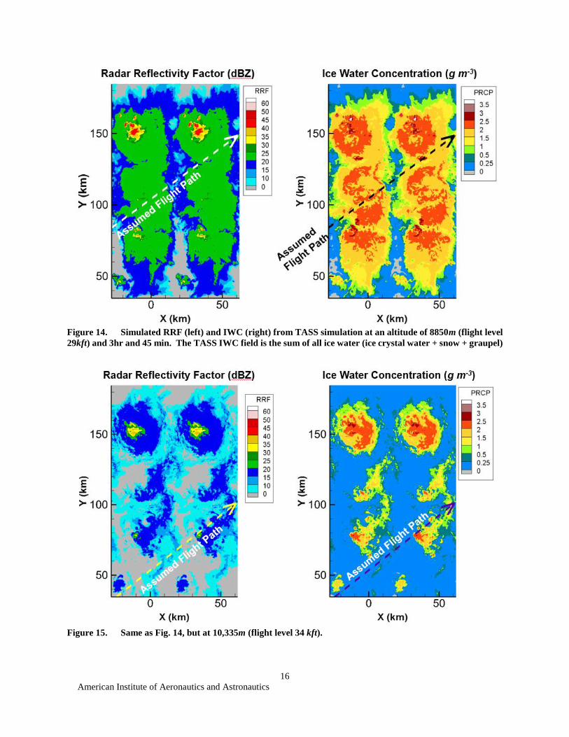
American Institute of Aeronautics and Astronautics
16
Figure 14 Simulated RRF (left) and IWC (right) from TASS simulation at an altitude of 8850m (flight level
29kft) and 3hr and 45 min The TASS IWC field is the sum of all ice water (ice crystal water + snow + graupel)
Figure 15 Same as Fig 14 but at 10335m (flight level 34 kft)
American Institute of Aeronautics and Astronautics
17
Figure 16 Comparison of RRF and IWC extracted along flight profiles shown in Figs 14 and 15 (dashed
lines) with those measured by the DC-8 (solid lines) Top row at an altitude of 8850m bottom row at 10350m
Figure 17 Two of the DC-8 legs with longest duration of IWC
Track of DC-8 superimposed on 1645 UTC GOES-13 Infrared
satellite imagery (Courtesy NASA Langley Satellite Group)
American Institute of Aeronautics and Astronautics
18
Figure 18 Vertical cross sections of RRF (top) and IWC (bottom) extrapolated from the numerical
simulation along the flight profile shown in Fig 14 Vertical position of both flight paths shown by dashed line
Altitudes are AGL
The numerical simulation does not capture the region of stratified precipitation that lies downstream from the
inflowing convective lines However the DC-8 flights did not encounter regions of HIWC when they overflew this
region It appears likely that the rain in this area was produced by moisture from the dissipation of the convective cells
and the overrunning of the cool surface dome by the moist southerly air currents A next-generation simulation would
need to include the horizontal variation of temperature and wind into the simulation in order to capture these effects
VI Numerical Simulation of Continental Supercell Hailstorm
In this section the numerical simulation of a continental supercell hailstorm is presented The purpose of this
simulation is to validate the robustness of the microphysics used in TASS and better understand differences in HIWC
production between continental supercell storms and subtropical MCS convection Validation parameters include 1)
production of large hail 2) size of hail swath 3) radar bounded weak echo region 4) supercell features 5) storm
motion 6) size and intensity of quasi-steady updraft 7) size and maximum value of radar echo and 8) duration In
this simulation we will verify the validity of the simulation by comparing our solutions with observed data In
addition this case will be analyzed for its potential in producing HIWC and compared with the previous case of
summertime coastal convection
This case has been simulated in the past with one of the first versions of TASS using a relatively coarse mesh
Even at this earlier stage of TASS development the simulation was able to capture many of the stormrsquos observed
features5934
A Description of Observed Case
On 2 August 1981 a very large and severe hailstorm moved across Southeastern Montana The storm was observed
during its mature phase with ground-based Doppler radars and with research aircraft as it moved through a network
of field instruments during the Cooperative Convective Precipitation Experiment60 (CCOPE) The storm quickly
developed many classical features of a supercell hailstorm It veered to the right of the environmental winds and
persisted for over 5 hours while leaving a wide swath of hail The storm was reported to have an intense quasi-steady
updraft with cyclonic rotation a low-level radar hook echo signature a mid-level bounded weak echo region (BWER)
signature (same as radar echo vault) damaging winds a broad swath of 1-3 cm diameter hail with some sizes as large
American Institute of Aeronautics and Astronautics
19
as 10 cm a mesolow or mesocyclone with a peak pressure drop of at least 6mb and a peak RRF between 65-75
dBZ61626364 The primary updraft of the storm was reported to be over 14 km wide and was located within the BWER
A research aircraft flew within the updraft at an altitude between 6 km and 75 km MSL they found nearly adiabatic
conditions with updraft speeds greater than 50 m s-1 liquid water droplet concentrations of up to 6 g m-3 and the
absence of precipitation-sized particles65 The lack of larger particles explained the very low magnitudes of RRF within
the BWER Hail was penetrated by the research aircraft on the western edges of the updraft in association with the
high reflectivity regions Weisman et al66 reported that the storm produced at least one funnel cloud and that some
damage reports were ldquosuggestiverdquo of tornadic activity Surface wind speeds were estimated between 50 to 100 mph
(20 to 45 m s-1)63
A special rawinsonde sounding was launched near the storm (Fig 19) and indicated an environment very favorable
for intense convection Convective indices
calculated from the sounding exhibited a CAPE of
almost 3500 J kg-1 and a lifted Index of -10oC
The sounding also indicated a tropopause height
of 109 km MSL (~99 km AGL) with a
temperature of -475oC and an equilibrium level
at 198 mb (123 km MSL) with a temperature of -
517oC According to the both the sounding and
aircraft observations the cloud base temperature
and height were about 136oC and 26 km MSL
respectively63 The ground was slightly less than
1km above sea level and varied somewhat with
location The wind profile for the sounding
exhibited a strong magnitude of helicity6768 and
vertical shearing of the environmental wind High
values of both helicity and CAPE are indicative of
supercell and tornadic storm environments The
presence of dry environmental air at storm mid-
levels likely inhibited any strong tornado
formation (eg Proctor et al33)
B Configuration
In numerical modeling of this system we apply the
same version of the TASS model as in the Coastal-MCS
case Differences are only due to grid and domain
configuration boundary conditions input sounding and
several input parameters that define the continental
aspects of the cloud droplets and the hail size
distribution All are discussed below
The domain is size is defined to be 150 km x 150 km
in the horizontal and 20 km in the vertical (Table 7) An
evenly spaced grid size of 200 m is assumed Open
lateral boundaries conditions are applied at all lateral
boundaries The ground surface is assumed flat and no
terrain features are included The domain uses the
TASS modelrsquos internal tracking algorithms17 in
order to move the grid with the lateral translation of
the storm
The initial state profiles for temperature
pressure wind and humidity are horizontally
uniform but vary vertically according to the input
sounding shown in Fig 19 Values representative of
contental Great-Plains systems are assumed to for
the cloud droplet concentration and for the hail size
distribution intercept parameter (Table 8)
Figure 19 Skew-T diagram representing environment for
2 August 1981 Special sounding observed near Knowlton
MT at 2356 UTC Environmental wind hodograph
inserted at bottom left
Table 7 Domain Size and Resolution
Domain Parameter Physical Dimension
Lateral dimensions (X Y) 150 km x 150 km
Vertical dimension (Z) 20 km
Lateral grid spacing 200 m
Vertical grid spacing 200 m
Computational grid ~56 x 10
6
grid points
Table 8 Initial Parameters
Cloud base height (AGL) 1700 m (740 mb)
Cloud droplet number density Ncd 800 droplets cm-3
HailGraupel particle size distribution intercept Noh
2 x 10⁴ m-4
American Institute of Aeronautics and Astronautics
20
The major diffences between the initial conditions of this case and the coastal MCS case are that this case
represents a more continental environment with stronger vertical wind shear less moisture but greater instability
C Comparison of Simulation with Observations
The numerical simulation is initiated at time zero by introducing a thermal impulse and integrating over 4 hours
of time The simulation produces a supercell hailstorm and captures many of the features observed in the real storm
These include large hail wide hail swath funnel cloud with damaging surface wind 15 km wide quasi-steady updraft
surrounded at storm-mid-level by a radar echo vault or BWER a radar hook echo signature right-rear quadrant gust
front massive overshooting tops and a large spreading anvil As can be see in Table 9 scales and intenisties match
very well between the observed and simulated event The simulated updraft velocity at 65 km MSL of 55 m s-1 matches
the peak value measured by a research aircraft that penetrated the storm at the same level As found from the aircraft
measurments the updraft core was nearly adiabatic with little or no precipitation The model simulation as in the
observational studies found most of the hail to be on the western and nortwestern edges of the primary storm updraft
Table 9 Comparison of observations with TASS for 2 August 1981 Supercell Hailstorm
Features Observed TASS Simulated Anvil Extent Downstream from Updraft
(based on Radar Echo) gt200 km gt150 km
Anvil Extent Upstream from Updraft gt20 km gt60 km
BWER Diameter ~75 km ~8 km
BWER Vertical Extent 10 75 km MSL 12-14 km MSL
Gust Front Location SW Flank SW Flank
Peak Gust Front Wind Speed gt20 ms 25 ms
Typical Hail Diameter at Surface 1-3 cm peak median diameter 2 cm
Hail Shaft Location Relative to Center of BWER 3-4 km West 4-6 km WNW
Width of Hail Swath 20-30 km 225 km
Supercell Lifetime gt 5 hrs gt 4 hrs
Persistent Low-Level Radar Hook Echo yes Yes
Maximum Liquid Cloud Water Content 65 g m-3 55 g m-3
Surface Pressure Drop 6 mb Mesocyclone 4 mb tornado 21 mb
Peak Rainfall Accumulation 30-35 mm 25 mm
Peak Radar Reflectivity Factor 75 dBZ 726 dBZ
Storm Movement (development stage) 260 at 10 ms 250 at 12 ms
Storm Movement (supercell stage) 282 at 18 ms 280 at 16 ms
Storm Top Overshoot above EL 3-4 km 5 km
Updraft Diameter 14-17 km 15 km
Max Updraft Velocity at 65 km MSL 53 ms 55 ms
Diameter of 20 dBZ Echo at 12 km MSL 45 km 45 km
Peak Surface-Level Gusts East of Updraft gt25 ms 30 ms
Radar Echo Top 16 km MSL 18 km MSL
Tornadoes Funnel cloud sighted Yes western side of mesocyclone
Peak Surface Wind Damage F1- wind damage (estimated 33-50 ms)
56 ms
Maximum Altitude of 10 dbZ Contour in BWER 6-8 km MSL 65 km MSL
American Institute of Aeronautics and Astronautics
21
Supercell environments often produce tornadoes or familes of tornadoes and a funnel cloud with surface wind
damage was reported with this system The funnel cloud that was produced in the numerical simulation was
intermittent and dissiapted when it moved into the cooler dryer air underneath the hail and rain shafts Tornado
formation in this simulation showed similar characteristics to those studied in an earlier paper where the presence of
dry mid-level air acts to weaken or suppress tornado formaition in supercell environments33
The time evolution of the area with RRF greater than 55 dBZ at an elevation of 5 km MSL (blue) and the peak
RRF anywhere in the storm (red) is shown in Fig 20 The peak RRF from the simulation matches the observations
very well For the area with RRF greater than 55 dBZ both observation and TASS show a ramp up in the first two
hours of the stormrsquos lifetime but the
simulation shows this area to be smaller
than detected by ground-based radar
A comparison of the supercell structure
from TASS with measurements from
ground-based radar are shown in Figs 21
and 22 Two horizontal levels of RRF are
shown one at 10 km MSL and the other at 4
km MSL The TASS simulation reproduces
many of the observed features and supercell
signatures including the BWER (ie radar
echo Vault (V)) the radar hook echo and
the radar echo streamer The scale of the
area covered by each intensity of RRF are
similar between TASS and observed as
well One contrast however is that the high-
reflectivity area within the hook echo region
appears larger in the observation than in the
simulation The area of highest reflectivity
which is west and northwest of the BWER
is associated with large hail in both
observation and simulation
In Fig 23 a vertical cross-section along
x-z coordinates is taken through the middle
of the BWER Again both the simulation and observation show similar features similar intensities and similar spatial
scales The BWER or radar Vault is clearly present in the simulation and extends deep into the storm The BWER
is located within the intense storm updraft and is produced by a lack of significant precipitation-sized particles
D HIWC Characteristics in Simulated Storm
The Montana supercell with its quasi-steady large diameter and intense updraft generates large volumes of ice
crystals that are transported into the upper regions of the troposphere Increasing wind speeds with height which is a
characteristic of supercell environments quickly transports many of the ice particles downstream within a large
expanding anvil cloud Hail and larger ice particles are also carried up to high altitudes by the strong updrafts but fall
out relatively close-by due to their significant fall velocities Therefore large values of RRF can be found at storm
upper-levels within proximity to the supercell updraft The RRF drops-off with distance from the updraft as the larger
particles fall out and the remaining smaller particles are carried downstream
A graphical representation of the cloud and precipitation fields from TASS is show in Fig 24 Overshooting tops
which are above the predominant supercell updraft can penetrate several kilometers into the stratosphere A large
anvil cloud spreads mostly downstream from the overshooting tops due to the strong westerly winds beneath the
tropopause (cf Fig 9) This anvil cloud covers many square kilometers and forms a large overhang of cloud material
downstream from the storm updraft Due to the intensity of the updraft some the anvil material is transported counter
to upper-level winds and produces a forward overhang upstream from the storm updraft
The coldest cloud tops (Fig 25) are associated with the overshooting tops above the intense storm updraft Cloud
tops at temperaturesheights near the equilibrium level expand over a large area downstream from the overshooting
tops Obviously in Fig25 the anvil expands northeastward beyond the boundaries of the model domain
Figure 20 Time evolution of the maximum RRF anywhere
in the storm (red) and the cross-sectional area of reflectivity
exceeding 55 dBZ at 5km MSL (blue) Observed values from
Miller et al63(solid) compared with TASS (dashed)
American Institute of Aeronautics and Astronautics
22
Figure 22 Same as Fig 21 but RRF at an elevation of 4 km MSL Left adapted
from Millerrsquos analysis of ground based Doppler radar right from TASS at
t=3hr07min
RRF (dBZ)
Figure 21 Horizontal cross-section of Radar reflectivity factor at an altitude of
10 km MSL Left adapted from Millerrsquos analysis of ground based Doppler radar62
right from TASS at t=3hr07min Both plots windowed to 50km x 50km area with
major tick every 10 km The Radar echo Vault or BWER identified with V
Figure 23 Same as Fig 21 but RRF along vertical west-east cross-section through
BWER Left adapted from Millerrsquos analysis of ground based Doppler radar right from
TASS at t=3hr07min Altitude in km AGL with major ticks every 1km along abscissa
American Institute of Aeronautics and Astronautics
23
Very similar features for the simulated Montana supercell storm can be seen in the observed visible satellite
imagery of the actual system (Fig 26) The overshooting tops are positioned near the southern end and the anvil
expands toward the north-northeast The horizontal dimension of the observed cloud anvil compared with the cloud
top depicted in Fig 25 are nearly identical
Figure 27 shows the simulated IWC and RRF along a horizontal cross-section taken at 10km MSL (9km AGL)
The size and shape of the system represented in the cross-section is consistent with the satellite imagery in Fig 26 In
Fig 27 most of the RRF greater than 20 dBZ is confined to area within a 50 km diameter centered about the primary
updraft and BWER Values of RRF between 15-20 dBZ cover large areas downstream for the overshooting tops
Figure 27 also shows vast areas with IWC greater than 1 g m-3 In fact areas with 1 g m-3 or greater can be found at
distances of up to 50 to 100 km away from the regions with the greatest storm RRF Our simulation seems to imply
that by avoiding the high reflectivity areas by 20 nautical miles (37 km) may not be sufficient for avoiding prolonged
HIWC exposures
Figure 24 Simulated cloud and precipitation surfaces within the full TASS domain Viewed from south
Figure 25 Cloud top temperatures from TASS at 3hr75 min (left) and 3hr45min (right) simulation
time Coldest temperatures associated with overshooting tops in southwestern quadrant of figure
American Institute of Aeronautics and Astronautics
24
To further explore the structure of the simulated storm
vertical cross-sections are extracted alone lines A-B and C-D
that that appear in Fig27 These cross sections are shown in
Figs 28 and 29 They also help illustrate where HIWC
conditions may be found relative to the storm
The cross-sections through A-B (Fig 28) are taken
northeastward through the storm updraft It shows strong
reflectivity surrounding the BWER and extending to the upper
levels of the storm High levels of IWC largely composed of
hail are brought to the ground on the southwestern side of the
storm updraft and at upper-levels surrounding the updraft
Aircraft routinely avoid these areas due to their high values of
RRF More of a factor to air traffic is that significant levels of
IWC that can be found over large areas within the cloud
canopy at great distances downstream from the stormrsquos high
reflectivity regions Furthermore the RRF within the canopy
are very low and could be undetectable with many airborne
weather radars
In Fig 29 a cross section is taken orthogonal to the
direction of the shearing anvil It is taken northwestward
between C and D along the edge of the areas with significant
IWC (Fig 27) This cross-section resides at least 70 km or
more from areas with high RRF Along this cross section IWC
greater 1 g m-3 can be seen to extend for over a 100 km length
The layer has a thickness that is several kilometers thick This
layer also consist of very weak RRF (lt 20 dBZ) and
underneath has no detectable radar reflectivity or precipitation
Both cross-sections show that a layer with HIWC can extend over large distances and with very weak RRF
Beneath this layer containing HIWC precipitation was rarely apparent and radar reflectivity not detectable One visual
queue sometimes recommended to pilots for helping to identify potential HIWC conditions is the presence of strong
to moderate RRF from rain beneath regions of HIWC This queue would not apply to a supercell storm such as this
This case of a continental supercell also demonstrates that HIWC risks may not be confined to just oceanic and
coastal MCS since regions of significant IWC may extend for large distances with little RRF
VII Discussion and Conclusion
Flight data and results from numerical simulations are analyzed to better characterize the HIWC threat for aircraft
and to improve our understanding of the relationship between HIWC radar and satellite signatures Flight
measurements with airborne radar and microphysical probes suggest that RRF alone may not be adequate for the
detection of HIWC conditions This fact also is reinforced from the numerical model simulations
The numerical simulations confirm that HIWC can be produced in contrasting environments In warm moist
coastal and oceanic environments large volumes of ice crystals can be pumped into the upper-troposphere by
regenerating convective plumes associated with a long-lasting system Cloud material carried in the upper-level
outflow from these plumes coalesces to form a large overhanging canopy and contain significant concentrations of
ice crystals Perhaps due to the weaker wind shear of these environments and the duration of the systems large
concentrations may accumulate over time
Our simulation of a large continental supercell shows it to have a large persistent and nearly adiabatic updraft
that also can pump large volumes of ice crystals in to the upper troposphere Vertical windshear with strong winds
aloft (which are an ingredient in producing supercells) can act to transport ice crystals over large areas We speculate
that the increase ventilation due to environmental wind shear may dilute the peak concentrations of IWC in supercells
Figure 26 Observed visible satellite imagery
from GOES-7 Northeastern Montana 2315
UTC 2 August 1981
American Institute of Aeronautics and Astronautics
25
Figure 27 Ice water content (left) and RRF (right) from TASS at an elevation of 10km MSL and 3hr45
min) simulation time Ice water content (g m-3) is sum of ice crystal snow and hail water content Units
for RRF are (dBZ)
Figure 28 Vertical cross section along A-B in Fig 27 Top is ice water content (g m-3) and bottom is RRF
(dBZ) Altitudes are above ground level
American Institute of Aeronautics and Astronautics
26
In our study the microphysics for snow is improved by using analyzed PSD data measured during the flight
campaign A new relationship is developed that relates the exponential size-distribution intercept for ice particles with
their water content In the past the value for the intercept has been assumed constant or a function of temperature
only The new relationship is a function of snow or ice water content as well as temperature and was used to improve
the microphysical submodels in TASS
The TASS model was then applied to contrasting types of convection and compared to available observations
This comparison seemed very good and demonstrated the model could be applied robustly to convection in different
types of environments Excellent results were achieved using only simple bulk parametrizations for microphysics
suggesting that models that are more complex may not be needed depending upon application The profiles of ice
water content and RRF extracted from the simulation compared reasonably well with the measurements by the DC-8
during penetrations of the coastal MCS although some differences in variability were noted The TASS model was
also used to simulate a specific supercell hailstorm with excellent comparison to measurements in terms structure
features scales and magnitudes
The numerical studies for both cases found that regions of significant IWC could extend above regions with little
or no RRF This would imply that moderate to high radar reflectivity might not always be underneath HIWC events
Yet to be investigated is the potential for HIWC detection using a combination of sensors and sources for
information (ie satellite and other weather data) Also unexplored is the ability to detect HIWC with advanced
airborne radar tools
Appendix Ice Crystal Size Distributions
Relationships between the ice crystal size distributions temperature and ice water content are needed for the
parameterization of microphysical submodels used in TASS These relationships could be useful in other applications
such as the understanding the radar reflectivity factor (RRF) due to ice crystals Dr Alexei Korolev processed the
particle size distribution (PSD) data69 from data collected at one-Hertz intervals during the DC-8 flights from a 2D-S
probe and a particle-imaging probe (PIP) The measured data was discretized into appropriate size bins and normalized
by the width of the corresponding bin This allowed for the direct comparison of the PSD data with different size
resolutions and common theoretical drop-size distributions (eg Marshall-Palmer70) The size resolution for the 2D-S
probe was10 μm and 100 μm for the PIP The range of particle measurements extends from 15 μm to 12845 mm The
Figure 29 Same as in Fig 28 but for position C-D in Fig 27
American Institute of Aeronautics and Astronautics
27
size of irregularly shaped ice particles as estimated from particle images may be defined in several different ways
The composite PSD data used the length of the particle parallel to the photodiode array commonly called Ly
An intercept (N0) and slope (λ) parameter were found from the data by using a least-squares method to fit an
exponential distribution through the measured PSD This was repeated for all times in a flight Relationships can then
be established for N0S vs ice water content (IWC) and atmospheric temperature
Our numerical modeling effort previously employed a relationship for Nos that is a function of temperature
only1017 Recall that our snow category represents the larger ice particles (excluding graupel and hail) and assumes
an inverse exponential size distribution whereas our cloud ice category only represents the smaller ice particles with
diameters less than about 200 um Using combined data measured from each day of the NASA deployment (Table 1)
and binning according to temperature a new relationship was determined for Nos that is a function of both temperature
and snow water content Ms
Log10 (Nos) = 744 ndash 00217 Tc +10526 Ms ndash 015 Ms2 +0004 Ms3 (A-1)
for Tcgt -55OC and Ms lt 4 g m-3
where Nos has units of m-4 Ms has units of g m-3 and Tc is temperature of the environment in centigrade The
relationship was fitted from the flight data as shown in Fig A1 and produces a larger intercept value for either colder
temperatures or increasing snow water content A higher intercept value translates into a distribution with overall
smaller particles lower radar reflectivity factor and slightly slower fall velocity Other parameterized microphysical
processes are affected by the assumption for Nos these include sublimation or deposition of snow particles and other
growth processes
Note that when Ms 0 the above relationship asymptotes to a relationship suggested by Woods et al71 who
derived their relationship from analyzing ice particles in wintertime precipitation occurring in the Pacific Northwest
Based on all ice particles they found the following relationship for No
Log10 (No ) = 753 ndash 00207 Tc (A-2)
Since their measured ice water contents ranged between 003 and 030 g m-3 it would have been difficult for them to
detect any dependency of No on ice water content
As a further check to the validity Eq (A-1) we compare the observed short-range RRF with the value estimated
from the measured IWC using the assumption of an inverse exponential size distribution with Eq (1) as
ZS [mm6m3] = 390 x 108 Ms175 Nos
-075 (A-3)
where the above assumes melted spherical particles and accounts for the differences in radar dielectric constants for
ice and water
The comparisons are shown in Fig A1 and illustrates the lack of correlation of radar reflectivity with snow water
concentration for values of snow water greater than about 1 g m-3
American Institute of Aeronautics and Astronautics
28
Figure A1 Ice particle distribution intercept NoS
vs ice water content for three temperature ranges
Data points derived from PSD distributions
measured during all 2015 DC-8 Flight Campaign
flights (ie Table 1) Blue curve represents medium
value Red curve is fit using Eq (A-1)
Figure A2 Radar reflectivity factor vs ice
water content for three temperature ranges
Data points of close-range RRF measured during
all 2015 DC-8 Flight Campaign flights (ie Table
1) Blue curve represents medium value Red
curve using Eqs (A-3) and (A-1)
American Institute of Aeronautics and Astronautics
29
Acknowledgments
This research is sponsored by the Advanced Air Transport Technology Project of NASArsquos Advanced Air Vehicles
Program The authors would like to acknowledge the contributing organizations that enabled the Florida HIWC Radar
Flight Campaign the FAA Aviation Research Division and Aviation Weather Division the NASA Aviation Safety
Program the Boeing Company Met Analytics Science Engineering Associates Environment Canada the National
Center for Atmospheric Research Honeywell and Rockwell Collins The authors also would like to thank Tom
Ratvasky (NASA Glenn Research Center) and Walter Strapp (Met Analytics) for their programmatic technical and
operational support and the NASA Langley Satellite Group for providing satellite images In addition thanks to
Alexei Korolev (Environment and Climate Change Canada) for processing the PSD data from raw data collected
during the flight test The numerical simulations were conducted using the Pleiades high-performance supercomputer
cluster of the NASA Advanced Supercomputing Division
References
1Mason JG Strapp JW and Chow P ldquoThe Ice Particle Threat to Engines in Flightrdquo AIAA 2006-206 doi10251462006-
206 2Mason JG and Grzych M ldquoThe Challenges Identifying Weather Associated with Jet Engine Ice Crystal Icingrdquo SAE
International 2011-38-0094 doi1042712011-38-0094 3Bravin M Strapp JW and Mason J ldquoAn Investigation into Location and Convective Lifecycle Trends in an Ice Crystal
Icing Engine Event Databaserdquo SAE International 2015-01-2130 doi1042712015-01-2130 4Addy HE Jr and Veres JP ldquoAn Overview of NASA Engine Ice-Crystal Icingrdquo SAE International 2011-38-0017
doi1042712011-38-0017 5Grandin A Merle J-M Weber M Strapp JW Protat A and King P ldquoAIRBUS Flight Tests in High Ice Water Content
Regionsrdquo AIAA 2014-2753 doi10251462014-2753 6Protat A and Rauniyar S Kumar VV and Strapp JW ldquoOptimizing the Probability of Flying in High Ice Water Content
Conditions in the Tropics Using a Regional-Scale Climatology of Convective Cell Propertiesrdquo Journal of Applied Meteorology
and Climatology Vol 53 November 2014 pp 2438-2456 doi101175jamc-d-14-00021 7Dezitter F Grandin A Brenguier JL Hervy F Schlager H Villedieu P and Zalamansky G ldquoHAIC (High Altitude
Ice Crystals)rdquo AIAA 2013-2674 doi10251462013-2674 8Houze RA Jr ldquoMesoscale Convective Systemsrdquo Review of Geophysics Vol 42 RG4003 2004 pp 1-43
doi1010292004RG000150 9Grzych M Tritz T Mason J Bravin M and Sharpsten A ldquoStudies of Cloud Characteristics Related to Jet Engine Ice
Crystal Icing Utilizing Infrared Satellite Imagerrdquo SAE International 2015-01-2086 doi1042712015-01-2086 10Proctor FH and Switzer GF ldquoNumerical Simulation of HIWC Conditions with the Terminal Area Simulation Systemrdquo
AIAA-2016-4203 doi10251462016-4203 11Houze RA Jr Cloud Dynamics Ed Academic Press 1993 573 pp doi101002qj49712051918 12FAA ldquoTurbojet Turboprop and Turbofan Engine Induction System Icing and Ice Ingestionrdquo February 2004 Advisory
Circular 20-147 doi104271510198 13Davison CR Strapp JW Lilie L Ratvasky TP Dumont C ldquoIsokinetic TWC Evaporator Probe Calculations and
Systemic Uncertainty Analysisrdquo AIAA 2016-4060 doi10251462016-4060 14Strapp JW Lilie LE Ratvasky TP Davison C and Dumont C ldquoIsokinetic TWC Evaporator Probe Development of
the IKP2 and Performance Testing for the HAIC-HIWC Darwin 2014 and Cayenne-2015 Field Campaignsrdquo AIAA 2016-4059
doi10251462016-4059 15Lilie LE Sivo CP and Bouley DB ldquoDescription and Results for a Simple Ice Crystal Detection System for Airborne
Applicationsrdquo AIAA 2016-4058 doi10251462016-4058 16Crum TD and Alberty RL ldquoThe WSR-88D and the WSR-88D Operational Support Facilityrdquo Bulletin of the American
Meteorological Society Vol 74 No 9 1993 pp 1669-1688 doi1011751520-0477
doi1011751520-0477(1993)074lt1669TWATWOgt20CO2 17Proctor FH ldquoThe Terminal Area Simulation System Volume I Theoretical Formulationrdquo April 1987 NASA CR-4046 18Proctor FH ldquoNumerical Simulation of Wake Vortices Measured During the Idaho Falls and Memphis Field Programsrdquo
14th AIAA Applied Aerodynamic Conference Proceedings Part II June 1996 AIAA 96-2496-CP pp 943-960
doi10251461996-2496 19Proctor FH ldquoInteraction of Aircraft Wakes from Laterally Spaced Aircraftrdquo AIAA 2009-0343 doi10251462009-343 20Proctor FH ldquoNumerical Simulations of an Isolated Microburst Part I Dynamics and Structurerdquo Journal of the
Atmospheric Sciences Vol 45 pp 3137-3160 doi1011751520-0469(1988)045lt3137nsoaimgt20co2 21Proctor FH and Bowles RL ldquoThree-Dimensional Simulation of the Denver 11 July 1988 Microburst-Producing Stormrdquo
Meteorology and Atmospheric Physics Vol 49 1992 pp 107-124 doi101007bf01025403 22Proctor FH 1989 ldquoNumerical Simulations of an Isolated Microburst Part II Sensitivity Experimentsrdquo Journal of the
Atmospheric Sciences Vol 46 15 July 1989 pp 2143-2165 doi1011751520-0469(1989)046lt2143nsoaimgt20co2
American Institute of Aeronautics and Astronautics
30
23Proctor FH Bracalente EM Harrah SD Switzer GF and Britt CL ldquoSimulation of the 1994 Charlotte Microburst
with Look-Ahead Windshear Radarrdquo Preprints 27th Conference on Radar Meteorology American Meteorological Society October
1995 pp 530-532 Paper-10B-7 24Proctor FH Hamilton DW and Bowles RL ldquoNumerical Study of a Convective Turbulence Encounterrdquo AIAA 2002-
0944 doi10251462002-944 25Ahmad NN and Proctor FH ldquoLarge Eddy Simulations of Severe Convection Induced Turbulencerdquo AIAA 2011-3201
doi10251462011-3201 26Han J Lin Y-L Schowalter DG Arya SP and Proctor FH ldquoLarge Eddy Simulation of Aircraft Wake Vortices within
Homogeneous Turbulence Crow Instabilityrdquo AIAA Journal Vol 38 February 2000 pp 292-300 doi1025142956 27Proctor F 2004 report H Hamilton DW and Han J ldquoWake Vortex Transport and Decay in Ground Effect Vortex
Linking with the Groundrdquo AIAA 2000-0757 doi10251462000-757 28Proctor FH Hamilton DW Rutishauser DK and Switzer GF ldquoMeteorology and Wake Vortex Influence on American
Airlines FL-587 Accidentrdquo April 2004 NASA TM-2004-213018 29Proctor FH ldquoNumerical Study of a Long-Lived Isolated Wake Vortex in Ground Effectrdquo AIAA 2014-2469
doi10251462014-2469 30Schowalter DG DeCroix DS Lin Y-L Arya SP and Kaplan ML ldquoPlanetary Boundary Layer Simulation using
TASSrdquo April 1996 NASA CR-198325 31DeCroix DS Lin Y-L and Schowalter DG ldquoCellular Convection Embedded in the Convective Planetary Boundary
Layerrdquo Journal of Wind Engineering and Industrial Aerodynamics Vol 67 pp 387-401 doi101016s0167-6105(97)00088-3 32Ding F Arya SP Lin Y-L ldquoLarge-Eddy Simulation of the Atmospheric Boundary Layer Using a New Subgrid-Scale
Model II Weakly and Moderately Stable Casesrdquo Environmental Fluid Mechanics Vol 1 2001 pp 49-69
doi101023a1011543715591 33Proctor FH Ahmad NN and Limon Duparcmeur FM ldquoNumerical Simulation of a Tornado Generating Supercellrdquo
AIAA 3012-0557 doi10251462012-557 34Proctor FH ldquoThe Terminal Area Simulation System Volume II Verification Experimentsrdquo April 1987 NASA CR- 4047 35Vreman AW ldquoAn Eddy-Viscosity Subgrid-Scale Model for Turbulent Shear Flow Algebraic Theory and Applicationsrdquo
Physics of Fluids Vol 16 October 2004 pp 3670-3681 doi10106311785131 36Proctor FH and Han J ldquoNumerical Study of Wake Vortex Interaction with Ground Using the Terminal Area Simulation
Systemrdquo AIAA 99-0754 doi10251461999-754 37Switzer G and Proctor F ldquoTerminal Area Simulation System Userrsquos Guide ndash Version 100rdquo January 2014 NASA TM-
2014-218150 38Proctor FH ldquoNumerical Simulation of Wake Vortices Measured During the Idaho Falls and Memphis Field Programsrdquo
14th AIAA Applied Aerodynamic Conference Proceedings Part II June 1996 AIAA 96-2496-CP pp 943-960
doi10251461996-2496 39Leonard BP MacVean MK and Lock AP ldquoThe Flux-Integral Method for Multidimensional Convection and Diffusionrdquo
Applied Mathematical Modeling Vol 19 1995 pp 333-342 doi1010160307-904x(95)00017-e 40van Leer B ldquoTowards the Ultimate Conservative Difference Scheme V A Second-Order Sequel to Godunovrsquos Methodrdquo
Journal of Computational Physics Vol 32 1979 pp 101-136 doi1010160021-9991(79)90145-1 41Ahmad NN and Proctor FH ldquoAdvection of Microphysical Scalars in Terminal Area Simulation System (TASS)rdquo AIAA
2011-1004 doi10251462011-1004 42Klemp JB and Wilhelmson R ldquoThe Simulation of Three-Dimensional Convective Storm Dynamicsrdquo Journal of the
Atmospheric Sciences Vol 35 June 1978 pp 1070-1096 doi1011751520-0469(1978)035lt1070tsotdcgt20co2 43Wang CY ldquoExact Solutions of the Navier-Stokes Equations ndash The Generalized Beltrami Flows Review and Extensionrdquo
Acta Mechanica Vol 81 1990 pp 69-74 doi101007bf01174556 44Switzer GF ldquoValidation Tests of TASS for Application to 3-D Vortex Simulationsrdquo October 1996 NASA CR-4756 45Bull JR and Jameson A ldquoSimulation of the Compressible Taylor Green Vortex using High-Order Flux Reconstruction
Schemesrdquo AIAA 2014-3210 doi10251462014-3210 46Chapelier J-B Plata MDLL and Renac F ldquoInviscid and Viscous Simulations of the Taylor-Green Vortex Using a Modal
Discontinuous Galerkin Approachrdquo AIAA 2012-3073 doi10251462012-3073 47DeBonis JR ldquoSolutions of the Taylor-Green Vortex Problem Using High-Resolution Explicit Finite Difference Methodsrdquo
AIAA 2013-0382 doi10251462013-382 48Ahmad N and Proctor FH ldquoSimulation of Benchmark Cases with the Terminal Area Simulation Systemrdquo AIAA 2011-
1005 doi10251462011-1005 49Lin Y-L Farley RD and Orville HD ldquoBulk Parameterizations of the Snow Field in a Cloud Modelrdquo Journal of Climate
and Applied Meteorology Vol 32 1983 pp 1065-1092 doi1011751520-0450(1983)022lt1065bpotsfgt20co2 50Rutledge SA and Hobbs PV ldquoThe Mesoscale and Microscale Structure and Organization of Clouds and Precipitation
VIII A Model for the ldquoSeeder-Feederrdquo Process in Frontal Rainbandsrdquo Journal of the Atmospheric Sciences Vol 40 May 1983
pp 1185-1206 doi1011751520-0469(1983)040lt1185tmamsagt20co2
American Institute of Aeronautics and Astronautics
31
51Berry EX and Reinhardt RE ldquoAn Analysis of Cloud Drop Growth by Collection Part I Double Distributionsrdquo Journal
of the Atmospheric Sciences Vol 31 October 1974 pp 1814-1824 doi1011751520-0469(1974)031lt1814aaocdggt20co2 52Berry EX and Reinhardt RE ldquoAn Analysis of Cloud Drop Growth by Collection Part II Single Initial Distributionsrdquo
Journal of the Atmospheric Sciences Vol 31 October 1974 pp 1825-1831
doi1011751520-0469(1974)031lt1825aaocdggt20co2 53Proctor FH 1989 ldquoNumerical Simulations of an Isolated Microburst Part II Sensitivity Experimentsrdquo Journal of the
Atmospheric Sciences Vol 46 15 July 1989 pp 2143-2165 doi1011751520-0469(1989)046lt2143nsoaimgt20co2 54Sekhon RS and Srivastava RC ldquoDoppler Radar Observations of Drop-Size Distributions in a Thunderstormrdquo Journal of
the Atmospheric Sciences Vol 28 September 1971 pp 983-994 doi1011751520-0469(1971)028lt0983droodsgt20co2 55Musil DJ ldquoComputer Modeling of Hailstone Growth in Feeder Cloudsrdquo Journal of the Atmospheric Sciences Vol 27
1970 pp474-482 doi1011751520-0469(1970)027lt0474cmohgigt20co2 56Smith PL Jr Myers CG and Orville HD ldquoRadar Reflectivity Factor Calculations in Numerical Cloud Models using
Bulk Parameterizations of Precipitationrdquo Journal of Applied Meteorology Vol 14 September 1975 pp 1156-1165
doi1011751520-0450(1975)0143C1156rrfcin3E20co2 57Rogers RR A Short Course in Cloud Physics Pergamon Press 1976 227 pp doi101007bf00876948 58Blanchard DO ldquoAssessing the Vertical Distribution of Convective Available Potential Energyrdquo Weather and Forecasting
Vol 13 No 3 September 1998 pp 870-877 doi1011751520-0434(1998)013lt0870atvdocgt20co2 59Proctor FH 1985 ldquoThree Dimensional Simulation of the 2 August CCOPE Hailstorm with the Terminal Areas Simulation
Systemrdquo Report of the International Cloud Modelling WorkshopConference World Meteorological Organization WMP Report
No8 Technical Document WMOTD-139 September 1986 pp 227-240 60Knight CA ldquoThe Cooperative Convective Precipitation Experiment (CCOPE) 18 May -7 August 1981rdquo Bulletin of the
American Meteorological Society Vol 63 No 4 April 1982 pp 386-398
doi1011751520-0477(1982)063lt0386tccpemgt20co2 61Wade CG ldquoA Preliminary Study of an Intense Thunderstorm Which Moved Across the CCCOPE Research Network in
Southeastern Montanardquo Preprints 9th Conference on Forecasting and Analysisrdquo American Meteorological Society 1982 pp 388-
395 62Miller LJ ldquoThe CCOPE Hailstorm of 2 August 1981rdquo Report of the International Cloud Modelling WorkshopConference
World Meteorological Organization WMP Report No8 Technical Document WMOTD-139 September 1986 pp193-198 63Miller LJ Tuttle JD and Knight CA ldquoAirflow and Hail Growth in a Severe Northern High Plains Supercell ldquo Journal
of the Atmospheric Sciences Vol 45 No 4 1988 pp 736 doi1011751520-0469(1988)045lt0736aahgiagt20co2 64Wang PK ldquoMoisture Plumes Above Thunderstorm Anvils and their Contributions to Cross-Tropopause Transport of Water
Vapor in Midlatitudesrsquo Journal of Geophysical Research Vol 108 No D6 4194 2003 doi1010292002jd002581 65Musil DJ Heymsfield AJ and Smith PL ldquoMicrophysical Characteristics of a Well-Developed Weak Echo Region in a
High Plains Supercell Thunderstormrdquo Journal of Climate and Applied Meteorology Vol 25 July 1986 pp 1037-1051
doi1011751520-0450(1986)025lt1037mcoawdgt20co2 66Weisman ML Klemp J Miller LJ ldquoModeling and Doppler Analysis of the CCOPE August 2 Supercell Storm Preprints
13th Conference on Severe Local Storms American Meteorology Society 1983 pp 223226 67Davies-Jones RP Burgess D and Foster M ldquoTest of Helicity as a Tornado Forecast Parameterrdquo Preprints 16th Conf
on Severe Local Storms American Meteorological Society 1990 pp 588ndash592 68Brooks HE Doswell CA III and Cooper J ldquoOn the Environments of Tornadic and Nontornadic Mesocyclonesrdquo
Weather Forecasting Vol 9 December 1994 pp 606-618 doi1011751520-0434(1994)009lt0606oteotagt20co2 69Korolev A and Sussman B ldquoA Technique for Habit Classification of Cloud Particlesrdquo Journal of Atmospheric and
Oceanic Technology Vol 17 August 2000 pp 1048-1057 doi1011751520-0426(2000)017lt1048atfhcogt20co2 70Marshall JS and Palmer WM ldquoThe Distribution of Rain-Drops with Sizerdquo Journal of the Atmospheric Sciences Vol 5
1948 pp 179-207 doi1011751520-0469(1948)005lt0165tdorwsgt20co2 71Woods CP Stoelinga MT and Locatelli JD ldquoSize Spectra of Snow Particles Measured in Wintertime Precipitation in
the Pacific Northwestrdquo Journal of the Atmospheric Sciences Vol 65 January 2008 pp 189- 205 doi1011752007jas22431
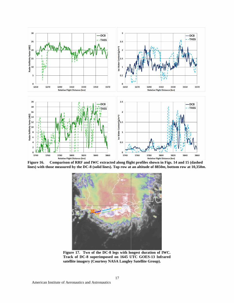
American Institute of Aeronautics and Astronautics
31
51Berry EX and Reinhardt RE ldquoAn Analysis of Cloud Drop Growth by Collection Part I Double Distributionsrdquo Journal
of the Atmospheric Sciences Vol 31 October 1974 pp 1814-1824 doi1011751520-0469(1974)031lt1814aaocdggt20co2 52Berry EX and Reinhardt RE ldquoAn Analysis of Cloud Drop Growth by Collection Part II Single Initial Distributionsrdquo
Journal of the Atmospheric Sciences Vol 31 October 1974 pp 1825-1831
doi1011751520-0469(1974)031lt1825aaocdggt20co2 53Proctor FH 1989 ldquoNumerical Simulations of an Isolated Microburst Part II Sensitivity Experimentsrdquo Journal of the
Atmospheric Sciences Vol 46 15 July 1989 pp 2143-2165 doi1011751520-0469(1989)046lt2143nsoaimgt20co2 54Sekhon RS and Srivastava RC ldquoDoppler Radar Observations of Drop-Size Distributions in a Thunderstormrdquo Journal of
the Atmospheric Sciences Vol 28 September 1971 pp 983-994 doi1011751520-0469(1971)028lt0983droodsgt20co2 55Musil DJ ldquoComputer Modeling of Hailstone Growth in Feeder Cloudsrdquo Journal of the Atmospheric Sciences Vol 27
1970 pp474-482 doi1011751520-0469(1970)027lt0474cmohgigt20co2 56Smith PL Jr Myers CG and Orville HD ldquoRadar Reflectivity Factor Calculations in Numerical Cloud Models using
Bulk Parameterizations of Precipitationrdquo Journal of Applied Meteorology Vol 14 September 1975 pp 1156-1165
doi1011751520-0450(1975)0143C1156rrfcin3E20co2 57Rogers RR A Short Course in Cloud Physics Pergamon Press 1976 227 pp doi101007bf00876948 58Blanchard DO ldquoAssessing the Vertical Distribution of Convective Available Potential Energyrdquo Weather and Forecasting
Vol 13 No 3 September 1998 pp 870-877 doi1011751520-0434(1998)013lt0870atvdocgt20co2 59Proctor FH 1985 ldquoThree Dimensional Simulation of the 2 August CCOPE Hailstorm with the Terminal Areas Simulation
Systemrdquo Report of the International Cloud Modelling WorkshopConference World Meteorological Organization WMP Report
No8 Technical Document WMOTD-139 September 1986 pp 227-240 60Knight CA ldquoThe Cooperative Convective Precipitation Experiment (CCOPE) 18 May -7 August 1981rdquo Bulletin of the
American Meteorological Society Vol 63 No 4 April 1982 pp 386-398
doi1011751520-0477(1982)063lt0386tccpemgt20co2 61Wade CG ldquoA Preliminary Study of an Intense Thunderstorm Which Moved Across the CCCOPE Research Network in
Southeastern Montanardquo Preprints 9th Conference on Forecasting and Analysisrdquo American Meteorological Society 1982 pp 388-
395 62Miller LJ ldquoThe CCOPE Hailstorm of 2 August 1981rdquo Report of the International Cloud Modelling WorkshopConference
World Meteorological Organization WMP Report No8 Technical Document WMOTD-139 September 1986 pp193-198 63Miller LJ Tuttle JD and Knight CA ldquoAirflow and Hail Growth in a Severe Northern High Plains Supercell ldquo Journal
of the Atmospheric Sciences Vol 45 No 4 1988 pp 736 doi1011751520-0469(1988)045lt0736aahgiagt20co2 64Wang PK ldquoMoisture Plumes Above Thunderstorm Anvils and their Contributions to Cross-Tropopause Transport of Water
Vapor in Midlatitudesrsquo Journal of Geophysical Research Vol 108 No D6 4194 2003 doi1010292002jd002581 65Musil DJ Heymsfield AJ and Smith PL ldquoMicrophysical Characteristics of a Well-Developed Weak Echo Region in a
High Plains Supercell Thunderstormrdquo Journal of Climate and Applied Meteorology Vol 25 July 1986 pp 1037-1051
doi1011751520-0450(1986)025lt1037mcoawdgt20co2 66Weisman ML Klemp J Miller LJ ldquoModeling and Doppler Analysis of the CCOPE August 2 Supercell Storm Preprints
13th Conference on Severe Local Storms American Meteorology Society 1983 pp 223226 67Davies-Jones RP Burgess D and Foster M ldquoTest of Helicity as a Tornado Forecast Parameterrdquo Preprints 16th Conf
on Severe Local Storms American Meteorological Society 1990 pp 588ndash592 68Brooks HE Doswell CA III and Cooper J ldquoOn the Environments of Tornadic and Nontornadic Mesocyclonesrdquo
Weather Forecasting Vol 9 December 1994 pp 606-618 doi1011751520-0434(1994)009lt0606oteotagt20co2 69Korolev A and Sussman B ldquoA Technique for Habit Classification of Cloud Particlesrdquo Journal of Atmospheric and
Oceanic Technology Vol 17 August 2000 pp 1048-1057 doi1011751520-0426(2000)017lt1048atfhcogt20co2 70Marshall JS and Palmer WM ldquoThe Distribution of Rain-Drops with Sizerdquo Journal of the Atmospheric Sciences Vol 5
1948 pp 179-207 doi1011751520-0469(1948)005lt0165tdorwsgt20co2 71Woods CP Stoelinga MT and Locatelli JD ldquoSize Spectra of Snow Particles Measured in Wintertime Precipitation in
the Pacific Northwestrdquo Journal of the Atmospheric Sciences Vol 65 January 2008 pp 189- 205 doi1011752007jas22431