high bit-rate digital communication through metal channels
TRANSCRIPT

High Bit-rate Digital Communication through Metal Channels
A Thesis
Submitted to the Faculty
of
Drexel University
by
Richard A Primerano
in partial fulfillment of the
requirements for the degree
of
Doctor of Philosophy
July 2010

c© Copyright July 2010Richard A Primerano. All Rights Reserved.

Table of Contents
List of Tables . . . . . . . . . . . . . . . . . . . . . . . . . . . . . . . . . . . . . . . . . . . . . . . . . . . . . . . . . . . . . . . . . . . . . . . . . . v
Abstract . . . . . . . . . . . . . . . . . . . . . . . . . . . . . . . . . . . . . . . . . . . . . . . . . . . . . . . . . . . . . . . . . . . . . . . . . . . . . . . . viii
1. Introduction . . . . . . . . . . . . . . . . . . . . . . . . . . . . . . . . . . . . . . . . . . . . . . . . . . . . . . . . . . . . . . . . . . . . . . . . 1
1.1 Objectives . . . . . . . . . . . . . . . . . . . . . . . . . . . . . . . . . . . . . . . . . . . . . . . . . . . . . . . . . . . . . . . . . . . . 3
1.2 Organization . . . . . . . . . . . . . . . . . . . . . . . . . . . . . . . . . . . . . . . . . . . . . . . . . . . . . . . . . . . . . . . . . 4
2. Motivating Example . . . . . . . . . . . . . . . . . . . . . . . . . . . . . . . . . . . . . . . . . . . . . . . . . . . . . . . . . . . . . . . 6
2.1 On-Ship Wireless Communication . . . . . . . . . . . . . . . . . . . . . . . . . . . . . . . . . . . . . . . . . . 6
2.2 Channel Echoes . . . . . . . . . . . . . . . . . . . . . . . . . . . . . . . . . . . . . . . . . . . . . . . . . . . . . . . . . . . . . . 9
2.3 Channel Capacity . . . . . . . . . . . . . . . . . . . . . . . . . . . . . . . . . . . . . . . . . . . . . . . . . . . . . . . . . . . . 13
2.4 Conclusion. . . . . . . . . . . . . . . . . . . . . . . . . . . . . . . . . . . . . . . . . . . . . . . . . . . . . . . . . . . . . . . . . . . . 15
3. Review of Related Technologies . . . . . . . . . . . . . . . . . . . . . . . . . . . . . . . . . . . . . . . . . . . . . . . . . . 16
3.1 Ultrasonic Communications . . . . . . . . . . . . . . . . . . . . . . . . . . . . . . . . . . . . . . . . . . . . . . . . . 16
3.2 Non-destructive Testing . . . . . . . . . . . . . . . . . . . . . . . . . . . . . . . . . . . . . . . . . . . . . . . . . . . . . 20
3.3 Communication Channel Equalization . . . . . . . . . . . . . . . . . . . . . . . . . . . . . . . . . . . . . 25
3.4 Application to the Present Work . . . . . . . . . . . . . . . . . . . . . . . . . . . . . . . . . . . . . . . . . . . 28
4. Ultrasonic System Model. . . . . . . . . . . . . . . . . . . . . . . . . . . . . . . . . . . . . . . . . . . . . . . . . . . . . . . . . . 30
4.1 Transducer-Bulkhead Decomposition. . . . . . . . . . . . . . . . . . . . . . . . . . . . . . . . . . . . . . . 30
4.2 Primary Path Model. . . . . . . . . . . . . . . . . . . . . . . . . . . . . . . . . . . . . . . . . . . . . . . . . . . . . . . . . 33
4.3 Echo Path Model . . . . . . . . . . . . . . . . . . . . . . . . . . . . . . . . . . . . . . . . . . . . . . . . . . . . . . . . . . . . 35
4.4 Channel Model Estimation. . . . . . . . . . . . . . . . . . . . . . . . . . . . . . . . . . . . . . . . . . . . . . . . . . 47
4.5 Model Validation . . . . . . . . . . . . . . . . . . . . . . . . . . . . . . . . . . . . . . . . . . . . . . . . . . . . . . . . . . . . 55
5. Basic Transceiver Designs . . . . . . . . . . . . . . . . . . . . . . . . . . . . . . . . . . . . . . . . . . . . . . . . . . . . . . . . . 64
5.1 Communication System Model . . . . . . . . . . . . . . . . . . . . . . . . . . . . . . . . . . . . . . . . . . . . . 64
5.2 Intersymbol Interference. . . . . . . . . . . . . . . . . . . . . . . . . . . . . . . . . . . . . . . . . . . . . . . . . . . . . 67
5.3 Echo Decay Envelope . . . . . . . . . . . . . . . . . . . . . . . . . . . . . . . . . . . . . . . . . . . . . . . . . . . . . . . . 69

5.4 Symbol/Echo Synchronization . . . . . . . . . . . . . . . . . . . . . . . . . . . . . . . . . . . . . . . . . . . . . . 75
5.5 Achievable Data Rate . . . . . . . . . . . . . . . . . . . . . . . . . . . . . . . . . . . . . . . . . . . . . . . . . . . . . . . 80
5.6 Summary . . . . . . . . . . . . . . . . . . . . . . . . . . . . . . . . . . . . . . . . . . . . . . . . . . . . . . . . . . . . . . . . . . . . . 92
6. Advanced Transceiver Designs . . . . . . . . . . . . . . . . . . . . . . . . . . . . . . . . . . . . . . . . . . . . . . . . . . . . 94
6.1 Channel Model Based Equalizer . . . . . . . . . . . . . . . . . . . . . . . . . . . . . . . . . . . . . . . . . . . . 94
6.2 Linear Equalizer . . . . . . . . . . . . . . . . . . . . . . . . . . . . . . . . . . . . . . . . . . . . . . . . . . . . . . . . . . . . . 104
6.3 Orthogonal Frequency Division Multiplexing . . . . . . . . . . . . . . . . . . . . . . . . . . . . . . 111
6.4 Summary . . . . . . . . . . . . . . . . . . . . . . . . . . . . . . . . . . . . . . . . . . . . . . . . . . . . . . . . . . . . . . . . . . . . . 116
7. Transceiver Hardware Implementation . . . . . . . . . . . . . . . . . . . . . . . . . . . . . . . . . . . . . . . . . . . 117
7.1 Transceiver complexity . . . . . . . . . . . . . . . . . . . . . . . . . . . . . . . . . . . . . . . . . . . . . . . . . . . . . . 118
7.2 Comparison of Techniques . . . . . . . . . . . . . . . . . . . . . . . . . . . . . . . . . . . . . . . . . . . . . . . . . . 126
Concluding Remarks . . . . . . . . . . . . . . . . . . . . . . . . . . . . . . . . . . . . . . . . . . . . . . . . . . . . . . . . . . . . . . . . . . 128
Bibliography . . . . . . . . . . . . . . . . . . . . . . . . . . . . . . . . . . . . . . . . . . . . . . . . . . . . . . . . . . . . . . . . . . . . . . . . . . . 130

i
List of Figures
1.1 Ultrasonic through-metal transceiver . . . . . . . . . . . . . . . . . . . . . . . . . . . . . . . . . . . . . . . . . . 1
2.1 Example wireless network . . . . . . . . . . . . . . . . . . . . . . . . . . . . . . . . . . . . . . . . . . . . . . . . . . . . . . . 6
2.2 Through metal data repeater . . . . . . . . . . . . . . . . . . . . . . . . . . . . . . . . . . . . . . . . . . . . . . . . . . . 7
2.3 Ultrasonic experimental setup . . . . . . . . . . . . . . . . . . . . . . . . . . . . . . . . . . . . . . . . . . . . . . . . . . 8
2.4 Channel transient response . . . . . . . . . . . . . . . . . . . . . . . . . . . . . . . . . . . . . . . . . . . . . . . . . . . . . 9
2.5 Basic echo cancelation. . . . . . . . . . . . . . . . . . . . . . . . . . . . . . . . . . . . . . . . . . . . . . . . . . . . . . . . . . . 10
2.6 Sources of echoing in the ultrasonic channel . . . . . . . . . . . . . . . . . . . . . . . . . . . . . . . . . . . 11
2.7 Basic echo cancelation. . . . . . . . . . . . . . . . . . . . . . . . . . . . . . . . . . . . . . . . . . . . . . . . . . . . . . . . . . . 12
2.8 Channel frequency response – without bulkhead . . . . . . . . . . . . . . . . . . . . . . . . . . . . . . 14
3.1 Redwood’s equivalent transducer model represented in PSpice . . . . . . . . . . . . . . 21
3.2 Gaussian pulse representing ultrasonic reflection. . . . . . . . . . . . . . . . . . . . . . . . . . . . . . 25
3.3 The Decision Feedback Equalizer. . . . . . . . . . . . . . . . . . . . . . . . . . . . . . . . . . . . . . . . . . . . . . . 27
4.1 End-to-end system block diagram . . . . . . . . . . . . . . . . . . . . . . . . . . . . . . . . . . . . . . . . . . . . . . 30
4.2 The components of the acoustic subsystem . . . . . . . . . . . . . . . . . . . . . . . . . . . . . . . . . . . . 31
4.3 Expanded and rearranged channel elements . . . . . . . . . . . . . . . . . . . . . . . . . . . . . . . . . . . 31
4.4 Channel partitioning . . . . . . . . . . . . . . . . . . . . . . . . . . . . . . . . . . . . . . . . . . . . . . . . . . . . . . . . . . . . 32
4.5 Gaussian pulses fitted to echo data . . . . . . . . . . . . . . . . . . . . . . . . . . . . . . . . . . . . . . . . . . . . 35
4.6 FDTD Analysis Mesh . . . . . . . . . . . . . . . . . . . . . . . . . . . . . . . . . . . . . . . . . . . . . . . . . . . . . . . . . . . 40
4.7 FDTD simulation, steel-aluminum .. . . . . . . . . . . . . . . . . . . . . . . . . . . . . . . . . . . . . . . . . . . . 42
4.8 FDTD results, steel-aluminum.. . . . . . . . . . . . . . . . . . . . . . . . . . . . . . . . . . . . . . . . . . . . . . . . . 43

ii
4.9 Determination of echo amplitude levels . . . . . . . . . . . . . . . . . . . . . . . . . . . . . . . . . . . . . . . . 44
4.10 FDTD simulation, steel-steel . . . . . . . . . . . . . . . . . . . . . . . . . . . . . . . . . . . . . . . . . . . . . . . . . . . 45
4.11 FDTD results, steel-aluminum.. . . . . . . . . . . . . . . . . . . . . . . . . . . . . . . . . . . . . . . . . . . . . . . . . 46
4.12 Transducer misalignment test results . . . . . . . . . . . . . . . . . . . . . . . . . . . . . . . . . . . . . . . . . . 47
4.13 FDTD simulation, steel-aluminum misaligned. . . . . . . . . . . . . . . . . . . . . . . . . . . . . . . . . 48
4.14 Input-output data generation . . . . . . . . . . . . . . . . . . . . . . . . . . . . . . . . . . . . . . . . . . . . . . . . . . . 49
4.15 Transmitted and First Received Pulses . . . . . . . . . . . . . . . . . . . . . . . . . . . . . . . . . . . . . . . . 51
4.16 First Received Pulses and First Echo . . . . . . . . . . . . . . . . . . . . . . . . . . . . . . . . . . . . . . . . . . 52
4.17 Complex envelope of received signal . . . . . . . . . . . . . . . . . . . . . . . . . . . . . . . . . . . . . . . . . . . 53
4.18 Representation of the acoustic channel in SIMULINKr . . . . . . . . . . . . . . . . . . . . . . 56
4.19 Frequency response of real and simulated channels . . . . . . . . . . . . . . . . . . . . . . . . . . . 57
4.20 Responses of physical and simulated system - single input pulse . . . . . . . . . . . . 58
4.21 Responses of simulated system - series of data pulses . . . . . . . . . . . . . . . . . . . . . . . . 59
4.22 Responses of physical and simulated systems - arbitrary pulse shape . . . . . . . 60
4.23 The two basis pulses used to test channel linearity . . . . . . . . . . . . . . . . . . . . . . . . . . . 62
4.24 The sum of the two shifted basis pulses is used to test additivity . . . . . . . . . . . 63
5.1 PAM received over an ideal ultrasonic channel . . . . . . . . . . . . . . . . . . . . . . . . . . . . . . . . 65
5.2 Components of the PAM communication system . . . . . . . . . . . . . . . . . . . . . . . . . . . . . 66
5.3 PAM received over non-ideal ultrasonic channel, contains ISI. . . . . . . . . . . . . . . . 68
5.4 ISI variation with symbol rate . . . . . . . . . . . . . . . . . . . . . . . . . . . . . . . . . . . . . . . . . . . . . . . . . . 69
5.5 Exponential echo decay . . . . . . . . . . . . . . . . . . . . . . . . . . . . . . . . . . . . . . . . . . . . . . . . . . . . . . . . . 71
5.6 Echo decay rate dependance on reflection coefficient . . . . . . . . . . . . . . . . . . . . . . . . . 72

iii
5.7 Interference bound for the exponential decay approximation . . . . . . . . . . . . . . . . 74
5.8 Interleaving symbols between echoes. tr = 6 tp, ts = 5 tp. . . . . . . . . . . . . . . . . . . . . . 77
5.9 Interleaving symbols between echoes. tr = 6 tp, ts = 3 tp. . . . . . . . . . . . . . . . . . . . . . 77
5.10 The ISI bound when considering symbol-echo synchronization . . . . . . . . . . . . . . 81
5.11 The PAM constellation . . . . . . . . . . . . . . . . . . . . . . . . . . . . . . . . . . . . . . . . . . . . . . . . . . . . . . . . . . 82
5.12 Bit error rate for unipolar PAM signaling . . . . . . . . . . . . . . . . . . . . . . . . . . . . . . . . . . . . . 84
5.13 Worst case ISI at symbol rate ts = τ . . . . . . . . . . . . . . . . . . . . . . . . . . . . . . . . . . . . . . . . . . . 85
5.14 Worst case ISI at symbol rate ts = 4τ . . . . . . . . . . . . . . . . . . . . . . . . . . . . . . . . . . . . . . . . . 86
5.15 The PAM constellation showing ISI bounds . . . . . . . . . . . . . . . . . . . . . . . . . . . . . . . . . . . 86
5.16 Bit error rate degradation with increase in ISI level . . . . . . . . . . . . . . . . . . . . . . . . . . 88
5.17 Bit rate as a function of SNR with Γ fixed at 0.48. . . . . . . . . . . . . . . . . . . . . . . . . . . . 90
5.18 Bit rate as a function of Γ with SNR fixed at 30 dB. . . . . . . . . . . . . . . . . . . . . . . . . . 91
5.19 PAM eye diagram with no equalization . . . . . . . . . . . . . . . . . . . . . . . . . . . . . . . . . . . . . . . . 92
6.1 Ultrasonic channel model . . . . . . . . . . . . . . . . . . . . . . . . . . . . . . . . . . . . . . . . . . . . . . . . . . . . . . . 95
6.2 Construction of the predistortion filter . . . . . . . . . . . . . . . . . . . . . . . . . . . . . . . . . . . . . . . . 96
6.3 Echo suppression using “basic” channel model . . . . . . . . . . . . . . . . . . . . . . . . . . . . . . . . 98
6.4 SINR improvement of 9 dB realized with simplified equalizer. . . . . . . . . . . . . . . . 99
6.5 The implementation of the simplified equalizer . . . . . . . . . . . . . . . . . . . . . . . . . . . . . . . 100
6.6 Bit rate as a function of SNR with Γ fixed at 0.48. . . . . . . . . . . . . . . . . . . . . . . . . . . . 101
6.7 PAM eye diagram when using simplified equalizer . . . . . . . . . . . . . . . . . . . . . . . . . . . . 102
6.8 The implementation of the advanced equalizer . . . . . . . . . . . . . . . . . . . . . . . . . . . . . . . . 102
6.9 Echo suppression using “advanced” channel model . . . . . . . . . . . . . . . . . . . . . . . . . . . 103

iv
6.10 PAM eye diagram when using improved equalizer . . . . . . . . . . . . . . . . . . . . . . . . . . . . 104
6.11 The Adaptive Linear Equalizer . . . . . . . . . . . . . . . . . . . . . . . . . . . . . . . . . . . . . . . . . . . . . . . . . 105
6.12 Convergence of linear adaptive PAM equalizer . . . . . . . . . . . . . . . . . . . . . . . . . . . . . . . . 107
6.13 Filter tap coefficients for PAM equalizer . . . . . . . . . . . . . . . . . . . . . . . . . . . . . . . . . . . . . . . 108
6.14 Signal constellation after convergence of QAM linear equalizer . . . . . . . . . . . . . . 110
6.15 Filter tap coefficients for QAM equalizer . . . . . . . . . . . . . . . . . . . . . . . . . . . . . . . . . . . . . . 110
6.16 Magnitude response of the ultrasonic channels . . . . . . . . . . . . . . . . . . . . . . . . . . . . . . . . 111
6.17 RMS noise measured on each OFDM subcarrier . . . . . . . . . . . . . . . . . . . . . . . . . . . . . . 114
6.18 OFDM subcarriers of differing constellation size . . . . . . . . . . . . . . . . . . . . . . . . . . . . . . 115
7.1 Hardware implementation common to all transceivers . . . . . . . . . . . . . . . . . . . . . . . . 117
7.2 Quadrature upconversion and downconversion processes . . . . . . . . . . . . . . . . . . . . . 118
7.3 Block diagram of Equalizer-free Transceiver . . . . . . . . . . . . . . . . . . . . . . . . . . . . . . . . . . 119
7.4 Envelope detector block diagram . . . . . . . . . . . . . . . . . . . . . . . . . . . . . . . . . . . . . . . . . . . . . . . 120
7.5 Block diagram of Channel Model based Transceiver . . . . . . . . . . . . . . . . . . . . . . . . . . 122
7.6 Block diagram of Linear Equalizer based Transceiver . . . . . . . . . . . . . . . . . . . . . . . . . 124
7.7 Block diagram of OFDM Transceiver . . . . . . . . . . . . . . . . . . . . . . . . . . . . . . . . . . . . . . . . . . 125

v
List of Tables
3.1 Ultrasonic comms systems found in the literature . . . . . . . . . . . . . . . . . . . . . . . . . . . . 19
4.1 Comparison of physical bulkhead and simulation model. . . . . . . . . . . . . . . . . . . . . . 56
7.1 Comparison of Transceiver Complexity . . . . . . . . . . . . . . . . . . . . . . . . . . . . . . . . . . . . . . . . 127

vi
List of Acronyms
A/D analog-to-digital converter
D/A digital-to-analog converter
DFE decision feedback equalizer
DSP digital signal processor
FIR finite impulse response
IIR infinite impulse response
ISI intersymbol interference
MAC multiply-accumulate
NDT non-destructive testing
PAM pulse amplitude modulation
RC raised-cosine
RRCF root raised-cosine filter
SNR signal-to-noise ratio
TDOA time difference of arrival
TTBR through the bulkhead repeater


viii
AbstractHigh Bit-rate Digital Communication through Metal Channels
Richard A Primerano
Advisor: Moshe Kam, Ph.D.
The need to transmit digital information across metallic barriers arises frequently
in industrial control applications. In some applications, the barrier can be penetrated
with wiring, while in others this may not be possible. For example, metal bulkheads,
pressure vessels, or pipelines may require a level of mechanical integrity that prohibits
mechanical penetration. This study investigates the use of ultrasonic signaling for
data transmission across metallic barriers, discusses the associated challenges, and
analyzes several alternative communication system implementations.
Several recent efforts have been made to develop through-metal ultrasonic commu-
nication systems, with approaches ranging widely in bitrate, complexity, and power
requirements. The transceiver designs presented here are intended to cover a range of
target applications. In systems having low data rate requirements, simple transceivers
with low hardware/software complexity can be used. At high data rates, however,
severe echoing in the ultrasonic channel leads to intersymbol interference. Reliable
high speed communication therefore requires the use of channel equalizers, and results
in a transceiver with higher hardware/software complexity.
In this thesis, issues related to the design of reliable through-metal ultrasonic com-
munication systems are discussed. These include (1) the development of mathematical
models used to characterize the channel, (2) application of equalization techniques
needed to achieve high-speed communication, and (3) analysis of hardware/software
complexity for alternative transceiver designs.
Several groups have developed through-metal ultrasonic communication systems
in the recent past, though none has produced a mathematical model that accurately

ix
describes the phenomena found within the channel. The channel model developed in
this thesis can be used at several stages of the transceiver design process, from trans-
ducer selection through channel equalizer design and ultimately system performance
simulation.
Using this channel model, we go on to develop and test several ultrasonic through-
metal transceiver designs. Ultrasonic through-metal communication systems are find-
ing use in a wide variety of applications. Some require high throughput, while others
require low power consumption. The motivation for developing several designs – rang-
ing from low complexity, low power to high complexity, high throughput – is so that
the best design can be matched to each application.
After these transceiver designs are developed, we present an analysis of their
computational requirements so that the most appropriate transceiver can be chosen
for a given application.


1
1. Introduction
The need to transmit digital information across metallic barriers arises frequently
in industrial control applications. For example, radio frequency sensing and control
networks deployed on naval vessels must maintain connectivity across multiple water-
tight bulkheads [1,2]. Since radio signals can not pass through the metal bulkhead, an
alternate method is needed to move data across it. Because the bulkhead is designed
to be watertight, penetrating it to install wires or cables is undesirable.
MetallicBarrier
Transducer
Driver
...0011101... ...0011101...
Recevier
Figure 1.1: Ultrasonic through-metal transceiver
The use of ultrasonic signaling to transmit digital information across metallic
barriers has been demonstrated by several groups [3–7]. Figure 1.1 illustrates the
concept of a through-metal ultrasonic transceiver, which is at the core of most exist-
ing efforts. Data entering a driver on the transmitting side of the system (left side
of the barrier) is encoded and used to drive a transmitting transducer transducer
that sends ultrasonic energy into the metallic barrier. The energy that reaches the

CHAPTER 1. INTRODUCTION 2
receiving transducer (right side of the barrier) is amplified by a receiver and from it,
the transmitted data sequence is recovered. In this thesis, issues related to the design
of reliable through-metal ultrasonic communication systems are discussed. These in-
clude (1) the development of mathematical models used to characterize the channel,
(2) application of equalization techniques needed to achieve high-speed communi-
cation, and (3) analysis of hardware/software complexity for alternative transceiver
designs.
This work originated as a means of providing connectivity to radio frequency
control networks on naval vessels, where ultrasonic through-metal transceivers would
ensure reliable communication across water tight (and RF shielding) bulkheads. Ad-
ditional applications of this technology include data transmission through pressure
vessels, pipe walls, and cargo containers. Recently, several efforts have been made
to transmit both data and power through metal using ultrasonic energy, allowing on
side of the transceiver to operate without battery power [8–10]. NASA has shown
interest in using this technology to monitor the contents of a sealed sample transport
container in its upcoming Mars Sample Return Mission [10]. As expected, in these
applications, low power consumption (and therefor low hardware/software complex-
ity) is important. In the remainder of this thesis, several ultrasonic transceiver designs
are presented that range in complexity and achievable data rate. In general, the de-
signs exhibiting lower complexity are best for low power, low data rate applications.
Higher complexity designs can support higher data rates at the expense of increased
power consumption. While this thesis does not address wireless power transmission,
it does develop the low complexity (low power consumption) transceiver designs that
are needed in such “batteryless” designs.

CHAPTER 1. INTRODUCTION 3
1.1 Objectives
This work provides a suite of digital communication algorithms, along with a hard-
ware testbed, that defines the tradeoffs between hardware/software complexity and
data rate in ultrasonic through-metal communication systems. The main components
are:
End-to-end Channel Model The through-metal communication system consists
of an interconnection of electrical and acoustic components. To understand the be-
havior of the system, these components have been individually modeled, and used
to form an end-to-end channel simulation. These models and simulation results are
useful in assessing the impact of transducer-barrier material mismatch and barrier
thickness variations, as well as determining the effect of different pulse shaping filters
and channel equalizers.
Application of Equalization Techniques Numerous channel equalization tech-
niques have been developed for use in telecommunications applications. These include
linear equalizers based on transversal filters [11], and nonlinear equalizers such as the
decision feedback equalizer [12]. Furthermore, these equalizers can be made adaptive
to cope with time-varying channel conditions [13]. One of the key differences between
the ultrasonic channel and most other telecommunications channels is that the inter-
ference present in the through-metal channel is well structured – a function of the
bulkhead’s material properties and dimensions. These properties of the ultrasonic
channel can be exploited to reduce equalizer complexity.
In addition to the commonly encountered equalization techniques, we present an
equalizer design method that uses a single training pulse to construct a model of
the ultrasonic channel, then uses that model to directly build an equalizing filter.
We show that in some applications this approach provides a low complexity solution

CHAPTER 1. INTRODUCTION 4
whose performance is equivalent to that of more complex, existing techniques.
Transceiver Complexity Analysis At the conclusion of this study, a summary
of relevant transceiver designs is presented, including details regarding the computa-
tional and hardware requirements of each solution. Since the through-metal commu-
nication techniques presented here may be deployed in a variety of applications with
differing throughput, cost, and power constraints, this analysis of throughput verses
transceiver complexity can help designers of through-metal communication systems.
1.2 Organization
This thesis is organized into seven chapters discussing the state-of-the-art in ultra-
sonic data communication, ultrasonic channel model development, transceiver design,
and hardware implementation issues. Chapters 2 through 7 provide the following in-
formation.
Chapter 2. Motivating Example An example application of the ultrasonic
through-metal transceiver is given, and an experimental laboratory test setup is de-
scribed. Experimental data gathered in the laboratory demonstrates the interference
issues present in the through-metal channel, and shows the origin of this interference.
Channel characteristics including signal-to-noise ratio (SNR) and bandwidth place
bounds on the channel’s achievable data rate.
Chapter 3. Review of Related Technologies Several past efforts toward the
development of through-metal ultrasonic communication systems are reviewed. Ad-
ditional topics related to ultrasonic communication system modeling and design are
reviewed as well. These include ultrasonic non-destructive testing and telecommuni-
cations channel equalizer design. This chapter summarizes the related technologies,
CHAPTER 1. INTRODUCTION 5
indicating how they apply the the present problem.
Chapter 4. Ultrasonic System Model A complete mathematical model of the
ultrasonic communication channel is developed. Variations in transducer bandwidth,
bulkhead thickness and makeup, and driving pulse shape can all be assessed through
a simulation of this model. The model is used in subsequent chapters to determine
the performance of different transceiver designs.
Chapter 5. Basic Transceiver Designs Ultrasonic transceivers designed for
low speed applications are presented. The echo characteristics of the channel are ana-
lyzed and an upper bound is placed on the intersymbol interference caused by echoes.
Using these results, a pulse-amplitude modulated (PAM) transceiver is designed and
its maximum achievable bitrate is determined.
Chapter 6. Advanced Transceiver Designs At high bitrates, equalization is
needed to combat intersymbol interference in the ultrasonic channel. In this chapter,
several equalizer structures are developed and applied. Adaptive filtering techniques
are implemented so that the equalizer can cope with time-varying channel character-
istics.
Chapter 7. Transceiver Hardware Implementation The transceiver designs
presented in prior chapters are compared in terms of hardware/software complexity
and achievable data rate. Based on throughput and power consumption requirements
of a particular application, the most appropriate transceiver design can be chosen.

6
2. Motivating Example
In recent years, the US Navy has expressed interest in deploying wireless sensing
and control networks on their vessels [14, 15]. These networks promise to decrease
the installation cost of machinery on ships while increasing survivability. The main
issue that has limited the use of wireless networks in the naval setting is their reliabil-
ity, namely, the difficulty in achieving reliable radio coverage throughout the vessel.
In this chapter, the use of ultrasonic through-metal transceivers is introduced as a
means of augmenting radio frequency wireless networks to increase their reliability.
Using a laboratory ultrasonic through-metal channel testbed, experimental results
are provided that illustrate the issues encountered in ultrasonic transceiver design.
2.1 On-Ship Wireless Communication
Figure 2.1 shows an example of a wireless temperature control system, consisting
of a controller, sensors, and actuators distributed across three RF isolated compart-
ments. In this closed-loop system, it is desired to keep the temperature of the water
exiting the heat exchanger constant. To accomplish this goal, a process controller
Compartment 1 Compartment 2 Compartment 3
Compressor
Boiler
HeatExchanger
ValveMotorDriver
ProcessController
Data Repeater
Figure 2.1: A wireless sensing network spanning multiple RF isolated compartments

CHAPTER 2. MOTIVATING EXAMPLE 7
reads the water temperature at the output of the heat exchanger and actuates the
control valve as needed. Each of these components communicates with other devices
within its compartments using radio frequency transceivers. Since the compartments
themselves are electromagnetically isolated from one another, a method of moving
data across them – to and from the process controller – is needed.
The through the bulkhead repeater (TTBR), shown in Figure 2.2, provides a bridge
between two wireless networks separated by an RF isolating bulkhead by passing data
ultrasonically across the bulkhead. This system requires no mechanical penetration
of the barrier.
Bulkhead
Ultrasonic Transducer
Wireless toUltrasonicTransceiver
Figure 2.2: Through metal data repeater
Figure 2.3 shows the experimental setup used to study the through-metal ultra-
sonic channel. It consists of two 6 MHz, 0.25 inch contact transducers1 separated by
a 0.25 inch thick steel plate. Between each of the transducers and the metal plate is a
layer of couplant gel2 designed to maximize the acoustic power transfer between the
two components. In this setup, the transmitting transducer is connected to a func-
1Panametrics NDT A112s non-destructive testing contact transducer [16,17].2Panametrics NDT D-12 gel type Couplant D.

CHAPTER 2. MOTIVATING EXAMPLE 8
tion generator and the receiving transducer is connected to an oscilloscope. Signal
generation and analysis are performed in MATLAB R©.
9
Channel Characterization
TransducersPanametrics NDT: model A112S-RM
Bulkhead¼” thick mild steel plate
Pulse Generator
Transmitter Receiver
Bulkhead
ScopeBulkhead Mockup
Transducer
Figure 2.3: Experimental setup demonstrating echoing in ultrasonic channel
The simplest method of transmitting data through the metal channel is by pulse
amplitude modulation (PAM) [18], where baseband symbols are encoded into pulses
of varying amplitude. The top plot of Figure 2.4 shows a 5 volt pulse used to excite
the transmitting transducer during testing. This pulse represents one data symbol
being sent through the channel. The bottom plot of Figure 2.4 shows the signal
at the receiving transducer. It consists of a primary received pulse (Primary RX)
followed by a series of echo pulses. The primary received pulse corresponds to the
transmitted data symbol, and the echoes may cause intersymbol interference (ISI)
with subsequent transmissions. At low symbol rates (tens of kilosymbols/second),
the echoes from successive symbols decay sufficiently fast so that ISI is not a concern.
As symbol rate increases (and pulses become more closely spaced), the echoes from
neighboring pulses cause ISI, which if uncorrected, may lead to symbol errors.
Under the assumption that the channel is linear and that the echoes in Figure 2.4

CHAPTER 2. MOTIVATING EXAMPLE 9
0 1 2 3 4 5 6 7−5
0
5
Vol
tage
(V
)Transmitted
0 1 2 3 4 5 6 7−200
−100
0
100
200
Time (µs)
Vol
tage
(m
V)
Primary RxEcho #1 Echo #2
Received
Figure 2.4: Initial investigation of channel behavior. a) Excitation of channel bysingle pulse. b) Response showing primary response and echoes
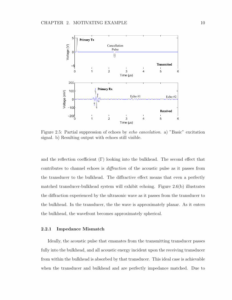
are time shifted, amplitude scaled versions of the primary received pulse, introducing
a cancelation pulse with corresponding time shift and amplitude scale should cause
complete suppression of echoes. Figure 2.5 shows the result of using this approach.
The echo amplitude is now about 4.5 dB below its original level, approximately 10 dB
below the primary. Residual echo energy remains because the amplitude response and
group delay of the channel are not flat.
2.2 Channel Echoes
We hypothesize that echoes observed in the ultrasonic channel’s transient response
are due to two effects. The first is impedance mismatch between the transducer and
bulkhead. As the impedance mismatch increases, the reflection coefficient magni-
tude at the junction between the transducer and bulkhead also increases. Figure
2.6(a) illustrates a rough contacting surface between the transducer and bulkhead,
CHAPTER 2. MOTIVATING EXAMPLE 10
CancellationPulse
Echo #1 Echo #2
Figure 2.5: Partial suppression of echoes by echo cancelation. a) ”Basic” excitationsignal. b) Resulting output with echoes still visible.
and the reflection coefficient (Γ) looking into the bulkhead. The second effect that
contributes to channel echoes is diffraction of the acoustic pulse as it passes from
the transducer to the bulkhead. The diffractive effect means that even a perfectly
matched transducer-bulkhead system will exhibit echoing. Figure 2.6(b) illustrates
the diffraction experienced by the ultrasonic wave as it passes from the transducer to
the bulkhead. In the transducer, the the wave is approximately planar. As it enters
the bulkhead, the wavefront becomes approximately spherical.
2.2.1 Impedance Mismatch
Ideally, the acoustic pulse that emanates from the transmitting transducer passes
fully into the bulkhead, and all acoustic energy incident upon the receiving transducer
from within the bulkhead is absorbed by that transducer. This ideal case is achievable
when the transducer and bulkhead and are perfectly impedance matched. Due to

CHAPTER 2. MOTIVATING EXAMPLE 11
Γ
Transducer Bulkhead
Couplant
(a) Impedance mismatch
Transducer Bulkhead
(b) Diffraction
Figure 2.6: Sources of echoing in the ultrasonic channel
material mismatch and surface roughness, an impedance mismatch (and reflection)
will always be present at the junction between transducer and bulkhead (Γ looking
into the bulkhead in Figure 2.6(a)).
While impedance mismatch can be reduced by carefully matching the transducer
to the bulkhead material and ensuring that the mating surfaces are very smooth, in
some applications neither step is practical. Matching the transducer to the material
properties of the bulkhead would require stocking a variety of transducer types (one
for steel, one for aluminum, ...), while grinding or lapping the mating surfaces to
ensure close contact would require special equipment that may not be available in
most installations.
2.2.2 Diffraction
The transmitting ultrasonic transducer is modeled as a piston source [19], since
the acoustic wave that emanates from its face is approximately planar. Figure 2.7
illustrates what happens as this wave enters the bulkhead (ignoring the impedance
mismatch between the two components). According to Huygens principle [20], the
acoustic wavefront at any time instant can be considered as a summation of point
sources, each giving rise to a spherical wavefront. The summation of these wavefronts
then describes the overall wavefront at some future time instant. For example, in

CHAPTER 2. MOTIVATING EXAMPLE 12
Figure 2.7, a plane wave emanating from the left hand transducer can be considered
an infinite series of point sources along the transducer’s face (only six are shown here).
The wavefront from each point source expands, and the overall wavefront is given by
their superposition. Diffraction causes the transmitted planar wavefront to become
approximately spherical (although the exact shape is dependant on the signal wave-
length relative to the transducer diameter) and as a result, not all of the transmitted
energy impinges on the receiving transducer’s face, even under perfect impedance
matching. The shape of the wavefront is determined by the ratio of transducer diam-
eter to bulkhead thickness. For d/t � 1 (thin bulkhead/wide transducer), the wave
is approximately planar. For d/t� 1 (thick bulkhead/narrow transducer), the wave
is approximately spherical.
t
d
Figure 2.7: The acoustic wavefront as it travels through the bulkhead, as explainedby Huygens principle
Several approaches have been developed to model ultrasonic transducers and wave
propagation in ultrasonic imaging/NDT applications [21–24]. Many models treat ul-
trasonic propagation as a one-dimensional effect, modeled with lumped element com-

CHAPTER 2. MOTIVATING EXAMPLE 13
ponents and transmission lines [21–23]. Other approaches model acoustic propagation
as a two or three-dimensional phenomenon [24]. We will show in Chapter 4 that while
impedance mismatch effects are captured by the one dimensional models, diffraction
effects are not.
2.3 Channel Capacity
Figure 2.4 shows that the ultrasonic channel’s transient response consists of a series
of echo pulses that result from acoustic energy being reflected within the bulkhead.
To develop an upper bound on channel data capacity, we first consider the capacity
supported by the channel with the bulkhead removed. This represents the presence of
an ideal equalizer (which eliminates the acoustic echoes) inserted into the system. The
channel’s capacity is a function of two quantities, signal-to-noise ratio and bandwidth3.
Signal-to-Noise Ratio (SNR) The channel’s signal-to-noise ratio at the ultra-
sonic receiver was calculated for the rectangular transmission pulse shown in Figure
2.4 – 70 ns width and 5 volts amplitude. The receiver output was first sampled with
no input signal applied to the channel, then with the rectangular pulse applied. The
two recorded waveforms were used to calculate noise power and signal plus noise
power, respectively,
Pn =1
T
∫T
|rn(t)|2dt Ps+n =1
T
∫T
|rs+n(t)|2dt, (2.1)
where rn(t) is the noise only received signal, rs+n(t) is noisy received symbol, and T
is the symbol period. In our testing, Ps+n/Pn ratios of 30 − 40 dB (1000 − 10000)
have been measured.
3The signal-to-noise ratio, bandwidth and bitrate values presented here are based on the physicalparameters of the test setup described in Figure 2.3.

CHAPTER 2. MOTIVATING EXAMPLE 14
Channel Bandwidth With the bulkhead removed and transmitting and receiving
transducers placed in direct contact, the magnitude response of the channel was
measured by transmitting a swept sinusoid and measuring the RMS value of the
received signal. Figure 2.8 shows the result of this test performed over the 3-16 MHz
range. This test reveals a 3 dB bandwidth of 2.9 MHz.
4 6 8 10 12 14 16−30
−20
−10
0
Frequency (MHz)
Mag
nitu
de (d
B)
Figure 2.8: Channel frequency response – without bulkhead
Capacity With the channel bandwidth, signal power, and noise power, an upper
limit on channel capacity can be calculated as
C = B log2
(1 +
PsPn
)= B log2
(Ps+nPn
)= 2.9 log2(1000) ≈ 29 Mbps.
(2.2)

CHAPTER 2. MOTIVATING EXAMPLE 15
Note that this channel capacity is a function of transducer choice (effecting band-
width) and transmission pulse shape (effecting SNR). In the following investigation,
we will continue to use the same transducer (the Panametrics NDT A112s 1/4” con-
tact transducer) but investigate alternate pulse shaping techniques, using the channel
capacity (Equation 2.2) as a benchmark.
2.4 Conclusion
The example in this chapter introduces the main impairment present in the ultra-
sonic channel – acoustic echoes. At high symbol rates, these echoes cause inter-symbol
interference. When no equalization is performed, the symbol rate of the channel pre-
sented in this chapter is limited to approximately 200K samples/second. When the
bulkhead is removed (eliminating echoes), the achievable symbol rate is on the order
of 2.9M samples/second (commensurate with the channel’s bandwidth). A properly
designed channel equalized can effectively remove the effect of the bulkhead (i.e. sup-
press echoes) allowing ISI free communication at this higher symbol rate.

16
3. Review of Related Technologies
The ultrasonic communication system combines new modeling and equalization
techniques with results from several existing research areas. This chapter provides
an overview of the existing body of work that has been applied to the through-metal
ultrasonic communication problem. This work includes topics from the fields of non-
destructive testing and telecommunications. We identify how the reviewed work was
extended to fit the unique requirements of our application.
3.1 Ultrasonic Communications
Ultrasonic signaling for digital communications has found widespread use in sev-
eral technological areas. The most common use has been in underwater communica-
tion systems. The severe multipath impairments that exist in this environment have
spurred the development of a host of new equalization techniques [25,26]. Ultrasonic
communication techniques have also been applied, to a lesser extent, to over-the-air
channels [27]. While similar multipath impairments exist in this environment, this
environment also suffers from high attenuation, limiting the usable range of such
communication systems [28]. Over the last several years, ultrasonic through-metal
communication systems have seen increasing interest [4]. Like the focus of the present
study, these systems are targeted at non-invasive data transmission across metallic
barriers whose structural integrity must be maintained.
3.1.1 Through-metal Communications
Beginning in the late 1990s, several groups have proposed using ultrasonic signal-
ing for data transmission through metal barriers [3,4,6,7,29–31]. These include several

CHAPTER 3. REVIEW OF RELATED TECHNOLOGIES 17
patent award [29–31]. The systems presented in the literature can be differentiated
based on their bit rate and power consumption. The applications cited include data
transmission through metal tanks and other “conductive envelopes” with thickness
of up to six (6) inches.
One of the first proposed through-metal data transmission systems appeared in
R. Welle’s 1999 patent [29]. The system claimed communication between an external
controller and an embedded sensor/actuator through an acoustic coupling medium,
though the patent makes no mention of modulation scheme, achievable data rate, or
implementation details.
One of the first peer-reviewed publications on the topic appeared in Saulnier et
al., 2006 [4]. This study focused on transmission of data across steel barriers up to
six inches thick. In the scenario presented, sensor data was conveyed from a sealed
metallic container to an outside relay. The main objective was to produce a low
complexity data repeater on the sensing side of the system so that power requirements
on the sensing side would be minimized, making battery powered operation possible.
A continuous wave was transmitted from the external transducer to the internal
(sensor side) transducer, and a change in the receiver side transducer’s load impedance
was used to modulate data on the reflected signal. This passive sensor-side modulation
can be accomplished with a relatively simple circuit as no transducer driver amplifier is
needed; a transistor placed across the sensor-side transducer acts as the variable load
impedance that will modulate reflected energy. The sensor-side hardware simplicity
adds complexity in the driver-side hardware. Several design implementations were
presented, using both pulse modulation and continuous wave modulation of data
between transmitter and receiver. In all cases, the main limiting factor in system
performance was acoustic echoing in the metal. The approach taken was to limit
data rate so that the ISI due to channel echoes was negligible. In the very thick

CHAPTER 3. REVIEW OF RELATED TECHNOLOGIES 18
specimens used in [4], this approach resulted in a data rate limitation of 450 bps.
The authors conclude by suggested that performance can be enhanced by using some
form of equalization.
One of the main contributions of [4] is the idea of moving transceiver complexity to
one side of the metal barrier. The low complexity side of the system being the sensor
side or the “interior,” and the high complexity side being the “exterior.” While the
system in [4] provides electrical power to both the internal and external transceivers,
the low hardware and computation complexity (and resulting low power requirement)
of the interior transceiver suggests that it may be supplied using a power harvesting
technique. The work presented in [5, 6] lays the groundwork for such techniques.
Extracting power from the ultrasonic signal generated from the exterior transceiver,
the interior transceiver can operate without battery power. Such systems are ideal
for sensing within sealed containers, where the sensor may remain inaccessible for
extended periods of time. Experimental results have shown a data rate of 55 kbps
and power transfer of 0.25 W in [5] and 1 kHz, 30 mW operation in [6].
The concept of ultrasonic power transmission predates any of the published work in
ultrasonic through-metal communication. One of the first published descriptions of a
system for recovering and storing electrical energy from ultrasonic energy appeared in
a 1997 patent [8]. Since this initial presentation of the concept, a more thorough anal-
ysis of ultrasonic power transmission system performance has been conducted [9,32].
This technique, coupled with the data transmission techniques discussed previously, is
being investigated for wireless monitoring in sample transport container for NASA’s
upcoming Mars Sample Return Mission [10].
Though the majority of the current research focuses on the use of piezoelectric
transducers for through-metal applications [4–6], at least one group has studied the
use of electromagnetic acoustic transducers (EMATs) instead [7]. These devices work

CHAPTER 3. REVIEW OF RELATED TECHNOLOGIES 19
on a completely different operating principle than piezoelectric transducers; they
induce a time varying Lorentz force in the metal specimen, that in turn sets up an
acoustic wave. However, as a communication channel this system functions identically
to its ultrasonic counterpart. Since EMATs induce an ultrasonic wave directly into the
specimen, they do not require the tight binding that piezoelectrics need. Their main
disadvantage is low conversion efficiency [33]. Their low efficiency translates into lower
power transmission capabilities, and lower SNR in data transmission applications.
Due to these limitations, the present study will focus exclusively on the use of lead
zirconate titanate (PZT) piezoelectric transducers.
3.1.2 Summary of Capabilities
Table 3.1 summarizes the capabilities of the ultrasonic data transmission systems
present in the literature. The table includes work done by our group as well, which
is be elaborated on throughout the remainder of this thesis.
Paper Bitrate Application Design FeaturesSaulnier, 2006 435 bps Low power/complexity Passive sensor-side modulationPrimerano, 2007 1 Mbps High speed/low complexity Echo cancellationShoudy, 2007 55 kbps Power harvesting Power harvesting, 250 mWKluge, 2008 1 kbps Sealed containers Power harvesting, 30 mWPrimerano, 2009 5 Mbps High speed Improved echo cancellationGraham, 2009 2 Mbps High speed Uses EMATs and equalization
Table 3.1: Comparison of ultrasonic communication systems found in the literature
Though channel echoing is recognized as the most significant impairment to high-
speed communication, most studies have not effectively dealt with the resulting ISI.
Beyond our initial work in echo cancelation and channel modeling, Graham [7] is the
only other source to have implemented any type of channel equalization for through-
metal ultrasonic communication.
CHAPTER 3. REVIEW OF RELATED TECHNOLOGIES 20
3.2 Non-destructive Testing
The ultrasonic through-metal communication channel is very similar to the axi-
ally aligned pitch-catch test configuration commonly used in non-destructive testing
(NDT) [21]. In this arrangement, two transducers are placed in an immersion tank
and directed toward one another, with the specimen under test placed between them.
Several authors have constructed end-to-end models of this type of ultrasonic test
setup [21, 22], and these results are applicable to the present work. By combining
these models, which account for transmitter and receiver amplifiers, cabling, trans-
ducers, and acoustic channel, with models of acoustic echoing, an end-to-end simula-
tion of our system can be constructed and used to design channel equalization filters.
In this section, we review the relevant literature in the area of ultrasonic transducer,
channel, and echo modeling.
3.2.1 Transducer Modeling
An ultrasonic transducer can be modeled as a two-port device; one port is electrical
and the other acoustic. The mathematical models discussed in this section relate the
voltage and current at the electrical port with the force and velocity at the acoustic
port. Several techniques are presented in the literature to derive these transducer
models, and they are briefly reviewed here.
Lumped-element Models The transducer’s physical construction can be used as
the basis for building an equivalent circuit model of the device. Several equivalent
circuit models have been proposed over the years, including Mason’s model [34] and
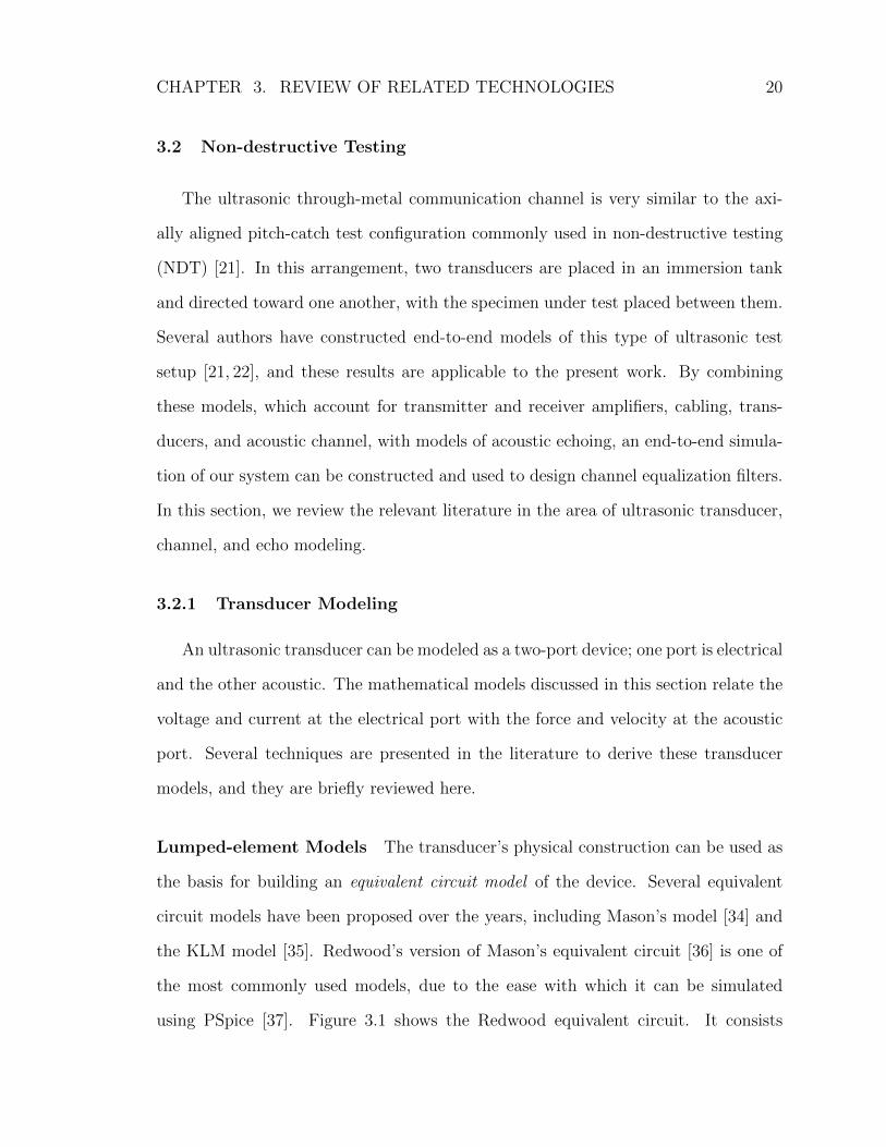
the KLM model [35]. Redwood’s version of Mason’s equivalent circuit [36] is one of
the most commonly used models, due to the ease with which it can be simulated
using PSpice [37]. Figure 3.1 shows the Redwood equivalent circuit. It consists

CHAPTER 3. REVIEW OF RELATED TECHNOLOGIES 21
of an electrical side and a mechanical side, coupled through a transformer. The
transmission line on the acoustic side accounts for the propagation delay of acoustic
signals through the transducer’s thickness. While the circuit is drawn as a three
port device (the voltage V , and two acoustic forces F1 and F2), one of the acoustic
terminals is generally matched to a permanently bonded backing material, allowing
the model to be treated as a two port device.
Figure 3.1: Redwood’s equivalent transducer model represented in PSpice
To apply the Redwood model requires that we map the physical parameters of
the transducer into the electrical parameters of the equivalent circuit. The model’s
electrical parameters are related to the transducer’s physical parameters through the
following relations [38–40].
Za = A√cDρo (3.1)
C0 = Aεs/l (3.2)
N = 1/C0h33 (3.3)

CHAPTER 3. REVIEW OF RELATED TECHNOLOGIES 22
where the following are properties of the piezoelectric ceramic; A - cross-sectional
area, cD - elastic stiffness constant, ρo - density, εs - dielectric constant, l - thickness,
h33 - piezoelectricity constant. The transducer’s physical parameters are available
from device manufacturers, or can be obtained through measurement. With these
electrical properties determined, the model is complete.
The presence of an unrealizable negative capacitance is perceived as a disadvantage
of this model, so several attempts have been made to simplify it. The Leach equivalent
model [23], based on the Redwood model, replaces the transformer with two current-
controlled current sources. The effect is to simultaneously eliminate the transformer
and the negative capacitance. Since its introduction, the Leach model has been widely
studied and simulated [41].
While other methods of transducer modeling have been developed, equivalent
circuit models have the advantage that they directly reflect the transducer’s physical
construction. The piezoelectric crystal’s capacitance, the acoustic transmission time
through the crystal, and the presence of matching layers can all be modeled directly
using lumped or distributed circuit components. System level models, consisting
of transmitter and receiver electronics, cables, and transducers, can all be directly
simulated in PSpice. Circuit based models are especially useful in transducer design.
Since variables such as crystal thickness and diameter, and matching layer material
are modeled explicitly, the circuit model provides insight into how changes in these
quantities affect transducer operation.
Black Box Models Equivalent circuit models directly model many of the internal
elements of an ultrasonic transducer. While such a representation is useful for trans-
ducer designers, the level of detail provided is often more than is required in many
applications. Furthermore, when working with commercial transducers, the equiva-
lent circuit component values are sometimes not available, as some manufacturers do

CHAPTER 3. REVIEW OF RELATED TECHNOLOGIES 23
not supply sufficient information to calculate them.
Several modeling techniques have been developed that use experimental data to
characterize the transducer. These “black box” models represent the transducer as a
transfer function or transmission matrix, abstracting the details found in the equiv-
alent circuit representation. In [21] the transducer is represented using the transfer
matrix in Equation 3.4, which relates acoustic force and velocity at the transducer’s
face to voltage and current at its terminals. The parameters of this transfer matrix
can be determined experimentally through electrical measurements using common
NDT test setups [42].
VI
=
TA11 TA12
TA21 TA22
Fv
(3.4)
In many NDT applications, users are interested only in determining the output
acoustic signal for a given excitation voltage. In [43], a method of recovering the
acoustic transfer function of the transducer using system identification is presented.
By applying an voltage signal to the transducer and measuring its response with a
hydrophone, system identification techniques can be used to approximate the transfer
function.
3.2.2 Acoustic Echo Modeling
We have shown in Chapter 2 that the transient behavior of the ultrasonic through-
metal communication channel consists of a series of echoes, corresponding to acoustic
energy reflected within the channel. In order to build an effective equalizer for this
channel, accurate estimation of the location and amplitude of these echoes must be
made. The accurate estimation of received pulse parameters (arrival time, amplitude,
spreading) is central to many ultrasonic imaging techniques, and many methods have

CHAPTER 3. REVIEW OF RELATED TECHNOLOGIES 24
been proposed to achieve high resolution time difference of arrival (TDOA) estimation
[44–46]. In this section, several of those methods are reviewed.
In ultrasonic TDOA estimation, the time difference between the transmission of a
reference pulse, and the reception of a reflected pulse is the quantity of interest. It is
common to assume that the reflected signal is identical to the reference signal, except
for a time delay, i.e. the reflected signal s(t) = r(t − τ) where r(t) is the reference
signals, and τ is the time delay between the two [45]. The simplest method of time
delay estimation is by locating a peak in the cross-correlation of the two signals.
Due to the computational complexity of this approach, however, researchers have
developed more efficient techniques that work well with high SNR signals [44]. In
ultrasonic time delay estimation, the relatively slow variations in echo characteristic
allow averaging of multiple consecutive echoes to be used to increase estimate accuracy
[45].
In many situations, the assumption that reflected signals are time shifted version
of the reference signal is not valid. Non-flat attenuation and group delay in the
acoustic medium will generally distort the reference signal causing the reflected signal
to be significantly different. Furthermore, the attenuation and delay properties of
the medium may be of interest, in addition to the the reflected signal’s time delay.
In medical imaging, for example, these properties may indicate the type of tissue
through which the signal passes [46]. Using a Gaussian echo model (Equation 3.5),
the reflected signal’s time delay and dispersion properties can be estimated.
s[θ;n] = β e−α (nT−τ)2 cos (2π fc (nT − τ) + φ)
θ = [α τ fc φ β ]
(3.5)
The Gaussian pulse, shown in Figure 3.2, is defined by five parameters: band-

CHAPTER 3. REVIEW OF RELATED TECHNOLOGIES 25
0 0.5 1 1.5 2 2.5 3
−1
−0.8
−0.6
−0.4
−0.2
0
0.2
0.4
0.6
0.8
1
Time (us)
Am
plitu
de (
volts
)
Figure 3.2: Gaussian pulse representing ultrasonic reflection
width factor (α), time delay (τ), center frequency (fc), phase (φ), and amplitude
(β). Estimation of these parameters amounts to fitting the model to experientially
gathered echo data [46]. In general, the reflected signal will contain multiple echo
components, each corresponding to a separate defect/discontinuity in the specimen
under test. This estimation technique has been extended to simultaneous estimation
of multiple echoes, and estimation of periodic echo trains [47]. Since the transient re-
sponse of the ultrasonic channel is characterized by an exponentially decaying (equally
spaced) pulse train, simultaneous estimation of multiple echoes is especially impor-
tant.
3.3 Communication Channel Equalization
The ultrasonic communication channel suffers from several impairments that are
commonly encountered in many other telecommunication systems. Acoustic echoes in

CHAPTER 3. REVIEW OF RELATED TECHNOLOGIES 26
the metal barrier lead to inter-symbol interference (ISI) while the resonant behavior
of the transducers results in a band limited channel. These phenomena were discussed
in Sections 2.2 and 2.3, respectively. The most common way of dealing with these
impairments is to construct an equalization filter placed in cascade with the channel.
Linear Equalizers The earliest channel equalizers for digital communication were
designed for data transmission over voice channels [18], and took the form of transver-
sal (tapped delay line) filters. The filter design problem amounts to proper selection
of filter taps so as to minimize some performance metric. The most common method
of choosing the tap coefficients of a transversal equalizers is to use the minimum
mean-square-error (MMSE) criterion [48]. Using this approach, tap coefficients are
selected to minimize the error criterion
J(c) = E|Ik − Ik|2, (3.6)
where Ik is the transmitted symbol, and Ik is the received symbol at the output of
the equalizer. It can be shown that J is a quadratic function of the tap coefficient
vector c [18], and therefore can be minimized using a variety of search methods –
the stochastic gradient method being one of the most popular. The MSE approach is
widely used in practice because it is robust in the face of high noise and large ISI [49].
Decision Feedback Equalizers Many communication channels containing strong
multipath components exhibit deep spectral nulls [18]. A linear equalizer combats
channel impairments by forming an approximate inverse of the channel’s response. As
a result, a channel with a spectra null at f0 will result in an equalizer having high gain
at that frequency. This high gain causes the equalizer to degrade SNR (referred to as
noise enhancement). To overcome this limitation, non-linear equalizer architectures

CHAPTER 3. REVIEW OF RELATED TECHNOLOGIES 27
have been developed. One of the most popular is the decision feedback equalizer
(DFE). A DFE tracks the last N symbols received, and uses that information to
cancel ISI from the symbol currently being received [50,51].
The structure of the DFE is shown in Figure 3.3. It consists of two filters, a
feedforward filter and a feedback filter. The feedforward filter is designed to compen-
sate for precursor ISI, while a feedback filter compensates for postcursor ISI. Noise
enhancement is avoided in the DFE because this equalizer does not attempt to in-
vert the entire channel response, only the portion that corresponds to postcursor ISI
(which is accomplished with the feedforward filter). Precursor ISI is canceled using
noiseless symbol decisions feed back from the slicer output.
Hf (f)
Hb(f)
x y
+
Figure 3.3: The Decision Feedback Equalizer
The two filters that form the DFE are usually implemented as tapped delay lines,
just as with the linear equalizer. The optimization of its filter coefficients can be
accomplished using the same procedures used for linear equalizer design. While de-
cision feedback equalizers outperforms linear equalizers in many applications, DFE
performance can quickly degrade in high noise channels. When the DFE feeds back
an incorrect symbol decision, error propagation can result. Basically, an incorrect
decision made on the currently received symbol increases the likelihood that the next
symbol will be interpreted incorrectly as well. It has been shown that error propaga-
tion leads to burst errors in the DFE’s output, which are generally self correcting [52].

CHAPTER 3. REVIEW OF RELATED TECHNOLOGIES 28
Adaptation Before an equalizer can function properly, it must be calibrated to the
channel over which it is to operate. The simplest method of calculating the proper
equalizer coefficients for a given channel is to send a known training sequence through
the channel, and measuring the error between the received symbol’s value and the
transmitted value [13]. The resulting error vector is then used to train the equalizer.
Using this approach, the equalizer can be retrained periodically by resenting the
training sequence at some interval. Alternatively, for channels that are slowly time
varying, the equalizer may implement an decision directed approach to continually
adapt [53] to the channel. A common approach to adaptive equalizer design is to first
train the equalizer using a training sequence, then switch to a decision directed mode
to provide on-line adaptation.
In some systems, the need to transmit a training sequence (which contains no use-
ful data) to tune the equalizer can add substantial overhead. As an alternative, blind
equalization techniques have been developed. An example of a blind equalization
technique is the constant modulus algorithm (CMA) [54]. Phase-shift keyed modula-
tion generates a carrier signal that has constant modulus (envelop). The CMA seeks
to adjust equalizer taps to achieve a constant modulus in the received signal. Any
deviation from constant modulus is used as an error signal that drives the adapta-
tion algorithm. In this way, equalizer adaptation can be performed without explicit
transmission of a training signal [13, 55].
3.4 Application to the Present Work
The ultrasonic through-metal communication environment shares similarities with
more commonly encountered (and more thoroughly studied) hardwired and radio
frequency channels. The interference experienced in the ultrasonic channel is similar
to wireless multipath fading, for example. A key difference in the ultrasonic channel

CHAPTER 3. REVIEW OF RELATED TECHNOLOGIES 29
is that interference is well structured, consisting of an exponentially decaying pulse
train. This can be used to our advantage to design particularly simple transceiver
architectures when low data rates are needed (the focus of Chapters 5). At high data
rates, more elaborate channel equalization techniques must be applied (the focus of
Chapters 6).
In recent years, several through-metal ultrasonic communication system designs
have emerged. No effort has been made to develop accurate mathematical models
of the ultrasonic channel, however. The topics presented in this chapter address
modeling and analysis of components of the ultrasonic communication channel. In
the following chapter, these will combined to form a complete channel model. In
particular, we will develop a transfer function that relates the electrical signal at
the input of the transmitting transducer to the electrical signal at the output of the
receiving transducer.

30
4. Ultrasonic System Model
In this chapter, mathematical models are developed for each of the components
that comprise the ultrasonic communication channel: transmitting transducer, bulk-
head, and receiving transducer. These models provide insight into the nature of
acoustic echoes, and allows us to test echo channel equalization techniques in simu-
lation. A block diagram of the ultrasonic communication system is shown in Figure
4.1.
Transmitter Transducer Bulkhead Transducer Receiverdata data
Figure 4.1: Block diagram of the ultrasonic communication system
The subsystem blocks shown in Figure 4.1 reflect the placement of components in
the ultrasonic communication system. In Section 4.5, we will show that the system
is linear, allowing us to rearrange blocks as needed to simplify modeling.
4.1 Transducer-Bulkhead Decomposition
We have observed that the transient response of the ultrasonic channel consists of
a primary received pulse followed by a series of echo pulses. Furthermore, the echo
portion of the response is what we seek to eliminate. Rather than develop explicit
models of the transmitting transducer, bulkhead, and receiving transducer, we will
first recast the transducer-bulkhead-transducer subsystem (which will be referred to
as the acoustic channel) into a form that models the primary pulse and echo pulses.
The acoustic channel is a cascade of three components, shown in Figure 4.2: the

CHAPTER 4. ULTRASONIC SYSTEM MODEL 31
Tt Bf Tr
Br
x y
+
Figure 4.2: The components of the acoustic subsystem
transmitting transducer (Tt), the bulkhead, and the receiving transducer (Tr). The
bulkhead is further decomposed into forward and reverse paths (Bf and Br respec-
tively), which accounts for the echoing observed in the system’s transient response.
The transfer function of the channel in Figure 4.2 in terms of these blocks is
Hc =TtBfTr
1−BrBf
(4.1)
Under the assumption of linearity (which will be discussed in Section 4.5), the
system can be expanded and rearranged into the representation shown in Figure 4.3.
This representation shows two signal paths. The first is through the transmitting
transducer, bulkhead forward path, and the receiving transducer. The second path
circulates from the output through the bulkhead reverse path, and the bulkhead
forward path. The latter accounts for channel echoes. It is straightforward to verify
that this representation is also described by Equation 4.1.
Tt Bf Trx y
BrBf
+
Figure 4.3: Expanded and rearranged channel elements

CHAPTER 4. ULTRASONIC SYSTEM MODEL 32
For convenience, the blocks in Figure 4.3 are grouped into two transfer functions.
P is the transfer function of the primary path, and E is the transfer function of
the echo path. With these definitions, the transfer function in equation 4.1 can be
rewritten as Equation 4.3.
Hc =TtBfTr
1−BrBf
=P
1− E(4.2)
P = TtBfTr, E = BrBf
The simplified channel block diagram in Figure 4.4 partitions the channel into two
subsystems. P relates the input pulse to the primary output pulse, and E relates
successive echo output pulses to one another.
Px y
E
+
Figure 4.4: Channel partitioned into primary (P ) and echo (E) subsystems
Rather than model the components in Figure 4.2 directly, we will base the acous-
tic subsystem’s model on the derived blocks in Figure 4.4. In addition to providing a
direct interpretation of the echoing phenomena in the channel, we will show in subse-
quent sections that models for these blocks can be easily extracted from experimental
data.

CHAPTER 4. ULTRASONIC SYSTEM MODEL 33
4.2 Primary Path Model
The primary signal path in the acoustic channel consists of the cascade of transmit-
ting transducer, bulkhead forward path, and receiving transducer, i.e. P = TtBfTr.
Extensive work has been done on modeling the individual components of the primary
path [21, 22,36, 43]. For example, [43] uses a system identification to extract a ratio-
nal transfer function approximation of the transducer. The equivalent circuit model
in [36] produces a PSPICE compatible simulation model of the transducer. Many of
the commonly used transducer modeling techniques are discussed in greater detail in
Section 3.2.1. In general, each of these two-port models relates an electrical signal at
one port of the transducer to an acoustic signal at the other port. In our application,
however, two transducers are placed back-to-back (with the bulkhead between them)
with the resulting system containing two electrical ports – the acoustic signals are
internal to the system. In this section, two methods of modeling the primary signal
path will be considered. The first is a frequency domain approach, while the second
is a time domain approach. Each method uses experimental channel input-output
data to form the model.
4.2.1 Transfer Function Model
Adapting the system identification technique used in [21, 43], which models the
electrical-acoustic transfer function of a single transducer, we have developed a method
of modeling the entire primary signal path (both transducers and the bulkhead froward
path) as a cascade of a rational transfer function and a pure delay, expressed as
P (z) = Pl(z)z−d. The lumped element portion of the transfer function, Pl(z), ac-
counts for the frequency selective effects of the transducers and bulkhead, while z−d
accounts for the acoustic delay contributed by those components. The form of Pl(z)

CHAPTER 4. ULTRASONIC SYSTEM MODEL 34
is given by Equation 4.4.
P (z) = Pl(z) z−d (4.3)
Pl(z) =bP (1) + bP (2)z−1 + · · ·+ bP (MP + 1)z−MP
aP (1) + aP (2)z−1 + · · ·+ aP (NP + 1)z−NP(4.4)
Using system identification techniques, the coefficient vectors bPbPbP and aPaPaP and the
time delay d can be determined from channel input-output data. The details of
the primary path modeling algorithm are presented in Section 4.4.2, including an
automated method of probing the channel and processing the resulting input-output
data used to estimate the parameters of Equation 4.3.
4.2.2 Analytical Pulse Model
The Gaussian pulse model was introduced in Section 3.2.2 as a model sometimes
used to describe the response of ultrasonic transducers in the time domain. The
pulse is defined by five parameters that control its amplitude, bandwidth, time offset,
resonant frequency, and phase.
s(t) = be−a(t−τ)2 cos (2π f (t− τ) + φ)
The Gaussian pulse modeling approach is particulary useful in estimating the
delay between two echo pulses, which indicates the round trip pulse time. Figure 4.5
shows the primary received pulse and first echo to emanate from the bulkhead,and a
pair of Gaussian pulses fitted to that data. An estimate of the round trip time can
be calculated once the pulses are fitted to the data, by taking the difference in the
delay values of the two pulses (i.e. ∆τ = τ2 − τ1).
Gaussian pulse fitting is especially useful for parametric detection of ultrasonic
echoes in low SNR environments. In our application, this time domain approach

CHAPTER 4. ULTRASONIC SYSTEM MODEL 35
0 0.5 1 1.5 2 2.5 3−1
−0.8
−0.6
−0.4
−0.2
0
0.2
0.4
0.6
0.8
1
Am
plitu
de (
volts
)
Time (µs)
Actual received signalFitted Gaussian pulses
Figure 4.5: Gaussian pulses fitted to two consecutive echoes
is used primarily for estimation of transducer center frequency and round-trip echo
time.
4.3 Echo Path Model
The second block of the acoustic channel – E(z) in Figure 4.4 – accounts for
the echo portion of the transient response. This block consists of the forward and
reverse bulkhead paths, modeling the dispersive effects of the bulkhead material,
the time delay of the acoustic signal traveling through the material, and the signal
reflections from the front and back faces of the bulkhead. Two modeling methods
will be presented in this section. In the first, the bulkhead is modeled as a cascade
of a rational transfer function and a delay element, just as was done in modeling the
primary path. This effectively treats the bulkhead as a one dimensional structure.
The second approach uses an analysis technique called Finite Difference Time Domain

CHAPTER 4. ULTRASONIC SYSTEM MODEL 36
(FDTD) simulation to model the true three dimensional propagation phenomena of
the bulkhead. While the former yields a simple, closed form model, the latter captures
propagation effects that are ignored by the one dimensional model.
4.3.1 Lumped Element Model
Following the same procedure that was used to model the primary signal path,
the echo path is assumed to be the cascade of a rational transfer function and an
ideal delay, E(z) = El(z)z−r. Here, the delay z−r accounts for the round trip acoustic
delay of the channel, and El(z) models the frequency selective effects of the bulkhead.
The form of El(z) is identical to that of the primary signal path’s lumped element
component.
E(z) = El(z) z−r (4.5)
El(z) =bE(1) + bE(2)z−1 + · · ·+ bE(ME + 1)z−ME
aE(1) + aE(2)z−1 + · · ·+ aE(NE + 1)z−NE(4.6)
The details of the echo path modeling algorithm are presented in Section 4.4.3,
including an automated method of probing the channel and processing the resulting
input-output data used to estimate the parameters of Equation 4.5.
4.3.2 Acoustic Propagation Simulation
The bulkhead model developed in Section 4.3.1 is a one-dimensional approxima-
tion of the three dimensional acoustic propagation within the bulkhead. As such,
some effects of the physical system are unmodeled. For example, in Section 6.1.2, we
will use this model to build an equalizer that should provide perfect cancelation of
channel echoes according to the one-dimensional model. In reality, a residual echo re-
mains, and can only be accounted for by considering a more detailed bulkhead model.

CHAPTER 4. ULTRASONIC SYSTEM MODEL 37
While impedance mismatch is the dominant mechanism for producing channel echoes,
diffraction (which the 1D model does not capture) experienced as the acoustic pulse
passes from the transducer to the bulkhead also leads to echoes, even under per-
fect acoustic impedance matching. In this section, we present a three-dimensional
simulation model that provides greater insight into the nature of channel echoes.
Acoustic Propagation The propagation of acoustic signals is governed by the
acoustic wave equation, a second order partial differential equation describing acous-
tic pressure and particle velocity as a function of both time and space. The finite
difference time domain (FDTD) method provides a means of approximating a so-
lution to the wave equation. This technique was first developed for electromagnetic
propagation simulation [56], but has since been extended to acoustic applications [57].
FDTD analysis is a grid based technique that begins by dividing the physical region
of interest into a series of cells and the time range of interest into time steps.
Consider an infinitesimal volume element of air being acted on by a pressure
gradient in the x-direction. The relationship between the element’s velocity, and the
pressure differential is described as
∂p
∂x= −ρ∂u
∂t(4.7)
where ∂p/∂x is the pressure gradient acting on the element, ρ is the density of the
material, and u is the element’s velocity. Note that this is analogous to the relation-
ship F = ma. The negative sign indicates that the element accelerates in a direction
opposite the pressure gradient.
The pressure gradient across the volume element causes the element to deform.
From Hooke’s law, we know that the stress and strain in an elastic medium (like
air) are linearly related. The relationship between the change in size of the volume

CHAPTER 4. ULTRASONIC SYSTEM MODEL 38
element and the corresponding change in pressure is given by
∂u
∂x= − 1
B
∂p
∂t(4.8)
where ∂u/∂x is the velocity differential across the element, B is the bulk modulus of
the material, and p is the pressure of the element. Note the correspondence between
this relationship and Hooke’s law, F = −kx.
Equations 4.7 and 4.8 form the basis of the FDTD method for acoustics. They
can be solved simultaneously for either pressure or velocity to yield two equivalent
forms of the acoustic plane wave equation,
∂2p
∂t2=B
ρ
∂2p
∂x2
∂2u
∂t2= −B
ρ
∂2u
∂x2.
The propagating characteristics of a homogenous elastic material can be com-
plectly described by its density and bulk modulus. From these parameters, two im-
portant quantities can be calculated, the wave propagation velocity (c) of the medium,
and the characteristic impedance (Z0) of the medium.
c =
√B
ρ(4.9)
Z0 =√ρB = ρc (4.10)
Where two dissimilar materials, a wave will experience a reflection if there is an
impedance mismatch between the materials. The acoustic reflection coefficient is
defined as
Γ =Z1 − Z0
Z1 + Z0
, (4.11)
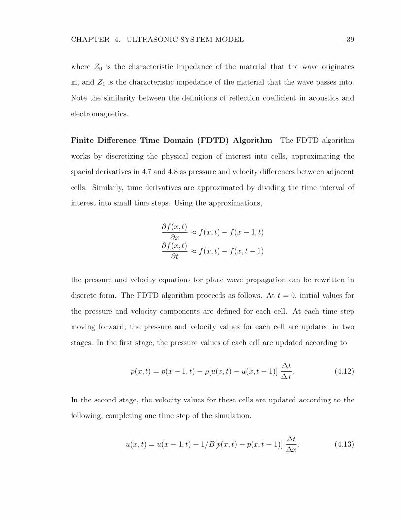
CHAPTER 4. ULTRASONIC SYSTEM MODEL 39
where Z0 is the characteristic impedance of the material that the wave originates
in, and Z1 is the characteristic impedance of the material that the wave passes into.
Note the similarity between the definitions of reflection coefficient in acoustics and
electromagnetics.
Finite Difference Time Domain (FDTD) Algorithm The FDTD algorithm
works by discretizing the physical region of interest into cells, approximating the
spacial derivatives in 4.7 and 4.8 as pressure and velocity differences between adjacent
cells. Similarly, time derivatives are approximated by dividing the time interval of
interest into small time steps. Using the approximations,
∂f(x, t)
∂x≈ f(x, t)− f(x− 1, t)
∂f(x, t)
∂t≈ f(x, t)− f(x, t− 1)
the pressure and velocity equations for plane wave propagation can be rewritten in
discrete form. The FDTD algorithm proceeds as follows. At t = 0, initial values for
the pressure and velocity components are defined for each cell. At each time step
moving forward, the pressure and velocity values for each cell are updated in two
stages. In the first stage, the pressure values of each cell are updated according to
p(x, t) = p(x− 1, t)− ρ[u(x, t)− u(x, t− 1)]∆t
∆x. (4.12)
In the second stage, the velocity values for these cells are updated according to the
following, completing one time step of the simulation.
u(x, t) = u(x− 1, t)− 1/B[p(x, t)− p(x, t− 1)]∆t
∆x. (4.13)

CHAPTER 4. ULTRASONIC SYSTEM MODEL 40
Note that for simplicity Equations 4.12 and 4.13 are written for a 1D plane wave case.
They can, however, be extended to 2D and 3D simulation.
Simulation Setup The FDTD simulation was conducted in Matlab. Though the
acoustic propagation phenomenon occurs in three dimensions, due to axial symmetry,
a 2D simulation gives identical results. Figure 4.6(a) shows the geometry and regions
defined for the simulation. Figure 4.6(b) shows how the geometry is divided using a
square mesh. Each cell of the mesh has its own density (ρ) and bulk modulus (B)
defined based on the material properties of that region.
Air
Transducer
Air
Bulkhead
Air
Transducer
Air
(a) Simulation geometry (b) Meshed geometry
Figure 4.6: The geometry and mesh used for the FDTD simulation
The transducer width and the bulkhead thickness are both 6 mm. The analysis
grid spacing is 0.1 mm, and the analysis region measures 20 mm x 15 mm. Each
simulation is run for one thousand time steps, approximately 14µs. An acoustic
source located at the leftmost face of the left side transducer. At each time step,
the acoustic force measured at the plane of each transducer (the face contacting the

CHAPTER 4. ULTRASONIC SYSTEM MODEL 41
bulkhead) was measured.
Simulation Results Using the setup described above, several simulations have
been performed to analyze the effect of material mismatch and transducer misalign-
ment on the channel’s transient response.
• Material Mismatch Transducers purchased for non-destructive testing are of-
ten designed to be matched to a particular type of material. Matching the char-
acteristic impedance of the transducer to the material being tested results in a low
reflection coefficient at the junction between transducer and specimen under test and
maximizes the power coupled from transducer to specimen. Impedance matching
between the transducer crystal and the specimen under test (or in our case, the bulk-
head) is usually done by bonding a quarter wavelength matching layer to the crystal
during manufacturing.
In our application, impedance mismatch causes not only poor power coupling,
but is also the major cause of channel reflections (and therefore ISI). Figure 4.7
illustrates simulation results where a transducer matched to aluminum has been used
with a steel bulkhead. Figure 4.7(a) shows the acoustic pulse originating within the
transmitting transducer. In Figure 4.7(b), the pulse has entered the bulkhead. Due to
the impedance mismatch between transducer and bulkhead, the reflection coefficient
at the interfaces between the two is Γ = −0.48. As a result, only portion of the
incident energy is coupled into the bulkhead. The remainder is reflected back into
the transmitting transducer. Figure 4.7(c) shows the acoustic pressure distribution
just after the transmitted pulse strikes the receiver side of the bulkhead. Again, a
portion of this signal passes into the transducer, and a portion is reflected back into
the bulkhead. Finally, in Figure 4.7(d), the signal is re-reflected from the transmitter
side of the bulkhead and travels back to the receiver side.

CHAPTER 4. ULTRASONIC SYSTEM MODEL 42
FDTD Acoustic AnalysisAluminum TransducerSteel Bulkhead, Γ = −0.48
time step 91 (1.3 µs)
Nor
mal
ized
Pre
ssur
e
−1
0
+1
(a) Simulation time = 1.3 µs
FDTD Acoustic AnalysisAluminum TransducerSteel Bulkhead, Γ = −0.48
time step 181 (2.5 µs)
Nor
mal
ized
Pre
ssur
e
−1
0
+1
(b) Simulation time = 2.5 µs
FDTD Acoustic AnalysisAluminum TransducerSteel Bulkhead, Γ = −0.48
time step 271 (3.8 µs)
Nor
mal
ized
Pre
ssur
e
−1
0
+1
(c) Simulation time = 3.8 µs
FDTD Acoustic AnalysisAluminum TransducerSteel Bulkhead, Γ = −0.48
time step 361 (5 µs)
Nor
mal
ized
Pre
ssur
e
−1
0
+1
(d) Simulation time = 5.0 µs
Figure 4.7: FDTD simulation, steel bulkhead and aluminum matched transducer
At each time step, the acoustic force measured at the face of each transducer
(where it contacts the bulkhead) is measured. Figure 4.8 shows the acoustic force at
the transmitting and receiving transducers over the duration of the simulation. Just
as with the experimental results, a strong primary received pulse is seen, followed by
an exponentially decaying series of echo pulses.
Using Equation 4.11, we determine that at the aluminum-steel interface, Γ =
−0.48 looking into the steel bulkhead. This value can also be determined from the
transient response when the exact material properties required by Equation 4.11 are

CHAPTER 4. ULTRASONIC SYSTEM MODEL 43
0 2 4 6 8 10 12 14−1
−0.5
0
0.5
1Transmitted
Nor
mal
ized
Am
plitu
de
0 2 4 6 8 10 12 14−1
−0.5
0
0.5
1Received
Time (µs)
Nor
mal
ized
Am
plitu
de
Figure 4.8: Acoustic force at transmitter and receiver faces, steel-aluminum
not known. Figure 4.9 illustrates the process of successive reflection in the bulkhead
and shows the amplitude level of the echoes after successive bounces, as well as the
amplitudes of the primary received pulse (ap) and first echo (ae) emanating from the
bulkhead. From the figure, we see that the ratio of these two quantities leads to
aeap
= Γ2 → Γ =
√aeap. (4.14)
By measuring the amplitudes of the first two pulses to emanate from the bulk-
head and using Equation 4.14, the value of the coefficient can be experimentally
determined. This relationship demonstrates that large acoustic mismatch leads to
large echo amplitude, and slow decay of the echo pulse train.

CHAPTER 4. ULTRASONIC SYSTEM MODEL 44
ai
ap = Tai – primary Gai
G2ai
ae = G2Tai – first echo
Figure 4.9: Determination of echo amplitude levels
• Perfect Transducer-Bulkhead Matching In the previous simulation, acous-
tic echoes were attributed to impedance mismatch between the transducer and bulk-
head. Next, we look at the case where the two are prefectly impedance matched – a
situation that can never quite be achieved in practice. Figure 4.10 shows four snap-
shots of this simulation at the same time steps as in the previous simulation. The
acoustic pulse generated by the transmitting transducer in Figure 4.10(a) enters the
bulkhead in Figure 4.10(b). In Figure 4.10(c), the incident acoustic pulse strikes the
receiver side of the bulkhead. The majority of the energy is coupled to the transducer,
but due to diffraction the pulse spreads while traveling, and some acoustic energy is
reflected back into the bulkhead. Note the circular wavefronts that emanate from the
top and bottom edges of the receiving transducer in Figure 4.10(c). Figure 4.10(d)
shows these wavefronts re-reflecting back toward the receiver side of the bulkhead.
This simulation reveals that even with perfect transducer-bulkhead matching,
echoes will still be present in the channel. This effect goes unmodeled in the transfer
function model (Equation 4.6). There are, in fact, two effects that contribute to chan-
nel echoes; impedance mismatch causes signal energy to reflect from the transducer-
bulkhead interfaces, while diffraction causes the spreading and reflection from the
edges of the transducers and the surrounding bulkhead. The acoustic pressure mea-
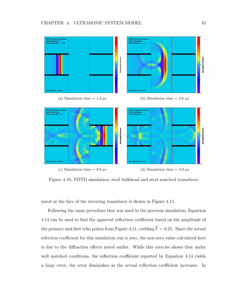
CHAPTER 4. ULTRASONIC SYSTEM MODEL 45
FDTD Acoustic AnalysisSteel TransducerSteel Bulkhead, Γ = 0.48
time step 91 (1.3 µs)
No
rmal
ized
Pre
ssu
re
−1
0
+1
(a) Simulation time = 1.3 µs
FDTD Acoustic AnalysisAluminum TransducerSteel Bulkhead, Γ = −0.48
time step 1000 (14 µs)
Nor
mal
ized
Pre
ssur
e
−1
0
+1
FDTD Acoustic AnalysisSteel TransducerSteel Bulkhead, Γ = 0
time step 181 (2.6 µs)
Nor
mal
ized
Pre
ssur
e
−1
0
+1
(b) Simulation time = 2.6 µs
FDTD Acoustic AnalysisAluminum TransducerSteel Bulkhead, Γ = −0.48
time step 1000 (14 µs)
Nor
mal
ized
Pre
ssur
e
−1
0
+1
FDTD Acoustic AnalysisSteel TransducerSteel Bulkhead, Γ = 0
time step 271 (3.9 µs)
Nor
mal
ized
Pre
ssur
e
−1
0
+1
(c) Simulation time = 3.9 µs
FDTD Acoustic AnalysisAluminum TransducerSteel Bulkhead, Γ = −0.48
time step 1000 (14 µs)
Nor
mal
ized
Pre
ssur
e
−1
0
+1
FDTD Acoustic AnalysisSteel TransducerSteel Bulkhead, Γ = 0
time step 361 (5.2 µs)
Nor
mal
ized
Pre
ssur
e
−1
0
+1
(d) Simulation time = 5.2 µs
Figure 4.10: FDTD simulation, steel bulkhead and steel matched transducer
sured at the face of the receiving transducer is shown in Figure 4.11.
Following the same procedure that was used in the previous simulation, Equation
4.14 can be used to find the apparent reflection coefficient based on the amplitude of
the primary and first echo pulses from Figure 4.11, yielding Γ = 0.25. Since the actual
refection coefficient for this simulation run is zero, the non-zero value calculated here
is due to the diffraction effects noted earlier. While this exercise shows that under
well matched conditions, the reflection coefficient reported by Equation 4.14 yields
a large error, the error diminishes as the actual reflection coefficient increases. In

CHAPTER 4. ULTRASONIC SYSTEM MODEL 46
0 2 4 6 8 10 12 14−1
−0.5
0
0.5
1Transmitted
Nor
mal
ized
Am
plitu
de
0 2 4 6 8 10 12 14−1
−0.5
0
0.5
1Received
Time (µs)
Nor
mal
ized
Am
plitu
de
Figure 4.11: Acoustic force at transmitter and receiver faces, steel-aluminum
the hardware testing presented later, we will see that very small values of Γ are
not achieved in practice (typical values are in the range of 0.45 − 0.65), and the
experimentally derived value (from Equation 4.14) is quite close to the actual value
(from Equation 4.11), within 5%.
• Transducer Misalignment The final simulation examines the effects of axial
misalignment between the transmitting and receiving transducers. Misalignments of
0−5 mm in 1 mm increments were examined using the aluminum-steel configuration.
The six curves in Figure 4.12(a) show the primary received pulses under misalign-
ments of 0− 5 mm. As misalignment increases, the energy coupled from transmitter
to receiver decreases. Figure 4.12(b) shows the power coupling from transmitter to
receiver as a function of misalignment. The results are normalized with respect to
zero misalignment. For the 6 mm wide transducers used in this simulation, a mis-

CHAPTER 4. ULTRASONIC SYSTEM MODEL 47
2.6 2.7 2.8 2.9 3 3.1 3.2 3.3 3.4 3.5 3.6
−0.5
0
0.5
1
Time (µs)
Nor
mal
ized
Am
plitu
de
d = 0 mmd = 1 mmd = 2 mmd = 3 mmd = 4 mmd = 5 mm
(a) Primary Rx pulses
0 0.5 1 1.5 2 2.5 3 3.5 4 4.5 50
0.2
0.4
0.6
0.8
1
Transducer offset distance (mm)
Rel
ativ
e po
wer
cou
plin
g
(b) Energy coupling vs. misalignment
Figure 4.12: Transducer misalignment test results
alignment of 2.5 mm causes a 3 dB reduction in coupled power and a misalignment
of 4.5 mm causes a 10 dB reduction in coupled power.
Figure 4.13 shows four frames of the 3 mm misalignment test, again at the same
time instants as the prior simulations. The simulation shows that the effect of mis-
alignment is to cause a large fraction of the transmitted energy to be reflected back
into the transmitting transducer.
4.4 Channel Model Estimation
In the previous sections, we discussed techniques for modeling the components of
the ultrasonic channel. In particular, the channel shown in Figure 4.4 has a transfer
function given by
Hc =P
1− E=
Pl(z)z−d
1− El(z)z−r, (4.15)
where Pl(z) and z−d are the lumped element and delay components, respectively, of
the primary path transfer function, while El(z) and z−r are the corresponding com-
ponents of the echo path transfer function. In this section, a technique for calculating

CHAPTER 4. ULTRASONIC SYSTEM MODEL 48
FDTD Acoustic AnalysisAluminum Trans\Steel Bulkhead2mm Misalignment, Γ = −0.48
time step 1000 (14 µs)
Nor
mal
ized
Pre
ssur
e
−1
0
+1
FDTD Acoustic AnalysisAluminum Trans\Steel Bulkhead3mm Misalignment, Γ = −0.48
time step 91 (1.3 µs)
Nor
mal
ized
Pre
ssur
e
−1
0
+1
(a) Simulation time = 1.3µs
FDTD Acoustic AnalysisAluminum Trans\Steel Bulkhead2mm Misalignment, Γ = −0.48
time step 1000 (14 µs)
Nor
mal
ized
Pre
ssur
e
−1
0
+1
FDTD Acoustic AnalysisAluminum Trans\Steel Bulkhead3mm Misalignment, Γ = −0.48
time step 181 (2.5 µs)
Nor
mal
ized
Pre
ssur
e
−1
0
+1
(b) Simulation time = 2.6µs
FDTD Acoustic AnalysisAluminum Trans\Steel Bulkhead2mm Misalignment, Γ = −0.48
time step 1000 (14 µs)
Nor
mal
ized
Pre
ssur
e
−1
0
+1
FDTD Acoustic AnalysisAluminum Trans\Steel Bulkhead3mm Misalignment, Γ = −0.48
time step 271 (3.8 µs)
Nor
mal
ized
Pre
ssur
e
−1
0
+1
(c) Simulation time = 3.9µs
FDTD Acoustic AnalysisAluminum Trans\Steel Bulkhead2mm Misalignment, Γ = −0.48
time step 1000 (14 µs)
Nor
mal
ized
Pre
ssur
e
−1
0
+1
FDTD Acoustic AnalysisAluminum Trans\Steel Bulkhead3mm Misalignment, Γ = −0.48
time step 361 (5 µs)
Nor
mal
ized
Pre
ssur
e
−1
0
+1
(d) Simulation time = 5.2µs
Figure 4.13: FDTD simulation, steel bulkhead and aluminum matched transducer,2mm misalignment
the parameters for these transfer functions using system identification is presented.
The top and bottom curves in Figure 4.14 show the input and output signals,
respectively, produced when the test setup in Figure 2.3 is excited with a 70 ns,
5 V amplitude rectangular pulse. In this section, a technique will be presented that
uses the transient response data along with system identification techniques to build
models for the primary and echo paths.

CHAPTER 4. ULTRASONIC SYSTEM MODEL 49
0 1 2 3 4 5 6 7−5
0
5
Vol
tage
(V
)Transmitted
0 1 2 3 4 5 6 7−200
−100
0
100
200
Time (µs)
Vol
tage
(m
V)
Primary RxEcho #1 Echo #2
Received
Figure 4.14: Channel transient response used to generate input-output data pairs
4.4.1 System Identification
System identification is the process of forming a mathematical model of a dynamic
system based on experimental data gathered from that system. System identification
is particularly useful when it is difficult or impractical to develop a system model based
on first principles. In such cases, black box models are used to describe the behavior
of a system. This approach was taken in developing the models in Equations 4.3 and
4.5, where we assumed the structure of each subsystem (rational transfer functions),
but did not determine values of the model coefficient. Presently, we consider how to
determine the values of these coefficients from experimental data.
Sending a known input signal x[n] into a physical system P (z) produces a mea-
sured output signal y[n]. Sending that same input x[n] into a model of that system,
denoted P (z), produces an output y[n]. The goal of system identification is to min-
imize the error between the actual system’s response, and that of the model. The
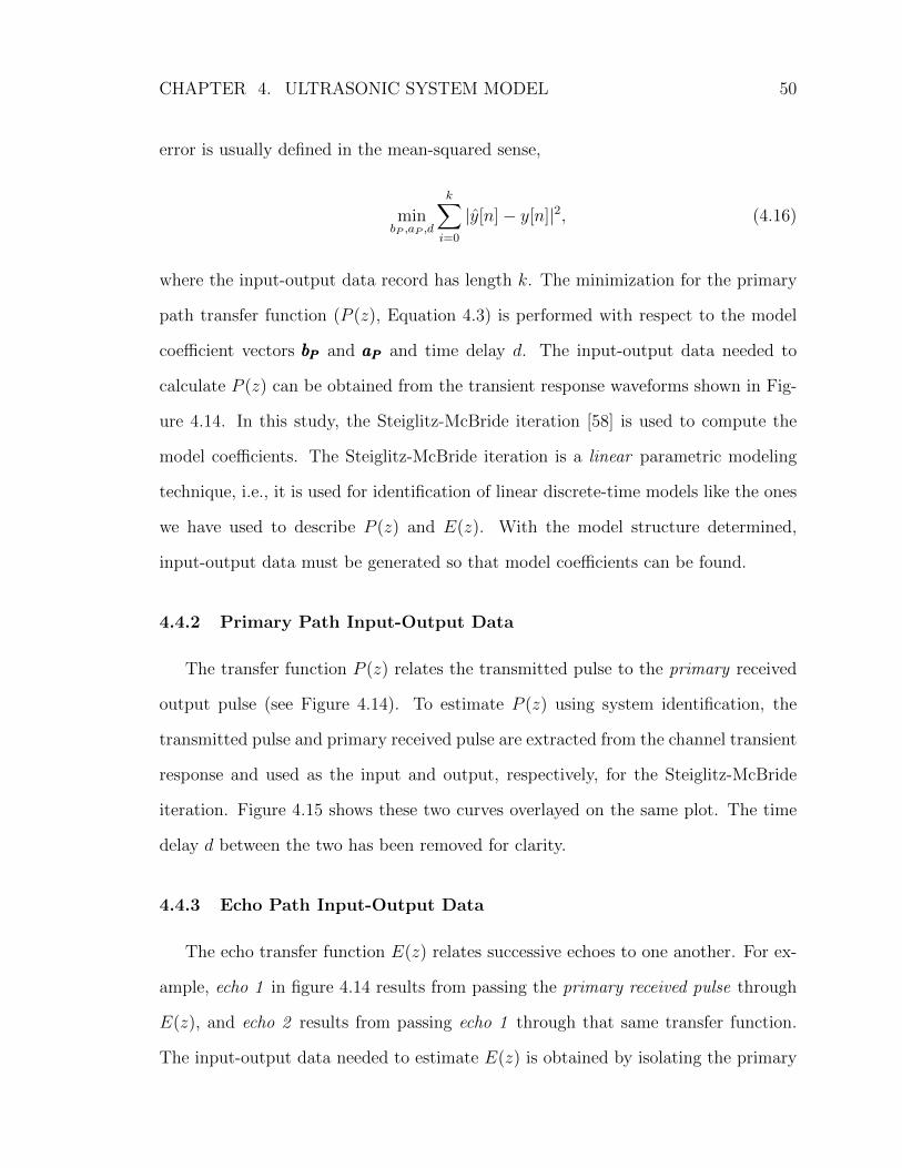
CHAPTER 4. ULTRASONIC SYSTEM MODEL 50
error is usually defined in the mean-squared sense,
minbP ,aP ,d
k∑i=0
|y[n]− y[n]|2, (4.16)
where the input-output data record has length k. The minimization for the primary
path transfer function (P (z), Equation 4.3) is performed with respect to the model
coefficient vectors bPbPbP and aPaPaP and time delay d. The input-output data needed to
calculate P (z) can be obtained from the transient response waveforms shown in Fig-
ure 4.14. In this study, the Steiglitz-McBride iteration [58] is used to compute the
model coefficients. The Steiglitz-McBride iteration is a linear parametric modeling
technique, i.e., it is used for identification of linear discrete-time models like the ones
we have used to describe P (z) and E(z). With the model structure determined,
input-output data must be generated so that model coefficients can be found.
4.4.2 Primary Path Input-Output Data
The transfer function P (z) relates the transmitted pulse to the primary received
output pulse (see Figure 4.14). To estimate P (z) using system identification, the
transmitted pulse and primary received pulse are extracted from the channel transient
response and used as the input and output, respectively, for the Steiglitz-McBride
iteration. Figure 4.15 shows these two curves overlayed on the same plot. The time
delay d between the two has been removed for clarity.
4.4.3 Echo Path Input-Output Data
The echo transfer function E(z) relates successive echoes to one another. For ex-
ample, echo 1 in figure 4.14 results from passing the primary received pulse through
E(z), and echo 2 results from passing echo 1 through that same transfer function.
The input-output data needed to estimate E(z) is obtained by isolating the primary

CHAPTER 4. ULTRASONIC SYSTEM MODEL 51
0 0.1 0.2 0.3 0.4 0.5 0.6 0.7 0.8 0.9 1
−1
−0.8
−0.6
−0.4
−0.2
0
0.2
0.4
0.6
0.8
1
Time (µs)
Nor
mal
ized
am
plitu
de
TransmittedReceived Primary
Figure 4.15: The transmitted pulse and primary received pulse aligned.
received pulse and first echo, and using those as the input and output data for the
Steiglitz-McBride iteration applied to E(z). Figure 4.16 shows these two curves over-
layed on the same plot. Again, the time delay between the two has been removed for
clarity.
4.4.4 Parameter Estimation Algorithm
The algorithm for estimating channel model parameters from the the channel’s
transient response is summarized in the following steps. In the following discussion,
model orders for P (z) and E(z) are assumed to be known and fixed. The issue of
model order estimation will be addressed subsequently.
1. Excite the channel with a step function and measure the resonant frequency of
the transducers.
2. Excite the channel with a pulse matched to the transducer’s resonant frequency

CHAPTER 4. ULTRASONIC SYSTEM MODEL 52
0 0.1 0.2 0.3 0.4 0.5 0.6 0.7 0.8 0.9 1
−1
−0.8
−0.6
−0.4
−0.2
0
0.2
0.4
0.6
0.8
1
Time (µs)
Nor
mal
ized
am
plitu
de
Received PrimaryReceived Echo #1
Figure 4.16: The primary received pulse and first echo aligned.
and record transient response.
3. Form initial estimate of channel round trip delay.
4. Extract primary received pulse and first echo from transient response.
5. Estimate parameters [bEbEbE aEaEaE r] of E(z) using extracted primary received pulse
and first echo.
6. Estimate parameters [bPbPbP aPaPaP d] of P (z) using known transmitted pulse and ex-
tracted primary received pulse.
The bulkhead is first excited with a step input then re-excited with an optimal
rectangular. The rectangular pulse has higher energy in the channel’s passband, and
results in a higher SNR received signal on which to perform parameter estimation.
The acoustic round trip time is then estimated by calculating the envelope of the
received pulse and locating the first two local maxima of that envelope. The distance

CHAPTER 4. ULTRASONIC SYSTEM MODEL 53
between these two points gives the estimated round trip time. Figure 4.17 shows
this estimation for a 0.635 cm thick steel bulkhead, with the two peaks marked by �
symbols.
2 2.5 3 3.5 4 4.5 5 5.5 6
−1
−0.8
−0.6
−0.4
−0.2
0
0.2
0.4
0.6
0.8
1
Time (µs)
Nor
mal
ized
am
plitu
de
Received SignalEnvelope
Figure 4.17: The complex envelope of the received signal with peaks marked
From Figure 4.17, the estimated round trip delay was 2.21 µs. This yields a
propagation speed of
c =2 ∗ 0.635 cm
2.21 µs= 5750 m/s,
which is consistent with published engineering data for the speed of sound through
steel. The envelope formed in Figure 4.17 is also used to extract the two echo pulses.
By searching to the left of the first peak for the envelope to decay to zero, the start
of the primary received pulse can be found. This point is shown in Figure 4.17 by
a ◦ symbol. With the start of the first received pause and the time between pulses

CHAPTER 4. ULTRASONIC SYSTEM MODEL 54
known, the first two received pulses can be extracted.
Next, the extracted pulses are used by the Steiglitz-McBride iteration to deter-
mine model parameters for E(z) and P (z). At the conclusion of the iteration, the
coefficients for the lumped element and time delay components of each block are
determined.
Offline Determination of Model Order Thus far, the orders of the numerator
and denominator terms in Pl(z) and El(z) have been assumed known. The order
of each transfer function is determined by the dynamic properties of the channel’s
primary and echo paths. For a given set of transducers and bulkhead, these orders
are fixed, however, they must be estimated at least once for each installation. We
have developed an algorithm to determine a suitable model order based on residual
mean-squared error between the channel response and model response. The steps
described below are in terms of Pl(z), but the same algorithm is used for estimating
the model order of El(z).
1. The system identification algorithm is run over a set of rational transfer function
models Pl(z : M,N), where the numerator (M) and denominator (N) orders are
noted explicitly. The residual error is recorded for each run.
2. An error threshold is set based on the smallest residual error from the group.
All models whose error exceeds that threshold are excluded.
3. Of the remaining models, the one with the smallest combined order (M + N)
is selected, and its order is chosen as the order for that subsystem.
For our system, the algorithm was iterated over the range of M ∈ {2, ..., 8} and
N ∈ {2, ..., 8}. The motivation for choosing the model with lowest combined order
(in step 3) is that this value relates directly to the number of multiply-accumulate

CHAPTER 4. ULTRASONIC SYSTEM MODEL 55
operations needed to calculate an output from the filter for each input. Thus, this step
results in choosing the least computationally complex model within the acceptable
residual error range. At the conclusion of the algorithm, the model orders for P (z)
and E(z) were found to be MP = 3, NP = 6 and ME = 3, NE = 2, respectively.
Using the laboratory testbed, the algorithm results in the following expressions for
the primary and echo transfer functions.
P (z) =−0.0004108 z−3 + 0.00183 z−4 − 0.002546 z−5 + 0.001137 z−6
1− 4.863 z−1 + 10.36 z−2 − 12.32 z−3 + 8.613 z−4 − 3.359 z−5 + 0.574 z−6z−110
E(z) =0.08627− 0.06211 z−1 − 0.05301 z−2 + 0.05128 z−3
z−1 − 1.705 z−2 + 0.864 z−3z−221
4.5 Model Validation
In this section, the ultrasonic channel model developed in Section 4.1 and tuned in
Section 4.4 is validated using experimental data gathered in the time and frequency
domains. Using such a model, the channel’s response to arbitrary inputs can be
simulated, including the response to digital waveforms. Furthermore, an accurate
simulation model allows us to assess the effects of various digital modulation and
equalization techniques. In subsequent chapters, the channel model will be used to
simulate the performance of several channel equalization algorithm.
The simulations presented here were performed in SIMULINKr, using the model
shown in Figure 4.18. Note the direct correspondence between this and the system
block diagram of Figure 4.4. The sample period used in the simulation is 100 ns
(fs = 100 MHz). The primary and echo paths are each represented by a cascade of a
delay element and a transfer function. The bulkhead’s round-trip delay is 221 samples,

CHAPTER 4. ULTRASONIC SYSTEM MODEL 56
or 2.21µs. This value matches the time delay estimated from Figure 4.17.
Rx1
Primary
P.b(z)
P.a(z)
Echo
E.b(z)
E.a(z)
Bulkhead Delay
-110Z
Bulkhead RTT
-221Z
Tx1
Figure 4.18: Representation of the acoustic channel in SIMULINKr
4.5.1 Frequency Response
In Chapter 2, it was illustrated that the introduction of the bulkhead into the
ultrasonic channel causes spectral nulls, associated with the standing wave pattern
within the bulkhead. Figure 4.19(a) shows a frequency sweep performed on the chan-
nel (with bulkhead in place) over the 0 − 22 MHz range, and Figure 4.19(b) shows
the same sweep conducted with the simulation model.
From the two plots several quantities can be measured. Values for channel center
frequency, null spacing, and null depth at center frequency are given in table 4.1.
Quantity Physical Simulation % errorCenter frequency 7.75 MHz 7.78 MHz 0.4 %Null spacing 460 kHz 458 kHz 0.4 %Null depth 6.70 dB 6.59 dB 2.5 %
Table 4.1: Comparison of measured quantities from physical bulkhead and simulationmodel

CHAPTER 4. ULTRASONIC SYSTEM MODEL 57
4 6 8 10 12 14 16−30
−20
−10
0
Frequency (MHz)
Mag
nitu
de (
dB)
(a) Physical channel
4 6 8 10 12 14 16−30
−20
−10
0
Frequency (MHz)
Mag
nitu
de (
dB)
(b) Simulated channel
Figure 4.19: Frequency response of real and simulated channels
4.5.2 Transient Response
The time domain behavior of the channel model has been tested with several
representative inputs. The accuracy of the model is determined by measuring the
error between the outputs of the physical and simulated systems when subject to the
same input.
Response to a single rectangular pulse The channel parameter estimation al-
gorithm uses a pulse matched to the channel’s resonant frequency as its excitation
signal. The top curve in Figure 4.20 show the response of the physical system when
excited with that pulse. The middle curve shows the output of the simulation model
(after estimating its parameters using the procedure in Section 4.4) when subject to
the same input pulse. As expected, the error between the two signals (bottom curve)
is small. The peak error between real and simulated outputs is less than 3% over the
duration of the output signal.

CHAPTER 4. ULTRASONIC SYSTEM MODEL 58
0 1 2 3 4 5 6 7 8 9 10−150
−100
−50
0
50
100
150
Vol
tage
(m
V)
Time (µs)
Physical
0 1 2 3 4 5 6 7 8 9 10−150
−100
−50
0
50
100
150
Vol
tage
(m
V)
Time (µs)
Simulation
0 1 2 3 4 5 6 7 8 9 10−150
−100
−50
0
50
100
150
Vol
tage
(m
V)
Time (µs)
Error
Figure 4.20: Responses of physical and simulated system - single input pulse
Response to data symbol sequence The results in Figure 4.21 show a more
interesting case where a series of pulses are transmitted in sequence. This is represen-
tative of using binary pulse-amplitude modulation (PAM) to to transmit the binary
sequence 1101011 at a symbol rate of 2µs. The top waveform shows the transmitted
sequence, and the middle waveform shows the simulated received sequence. This sim-
ulation clearly demonstrates the intersymbol interference introduced by closely spaced
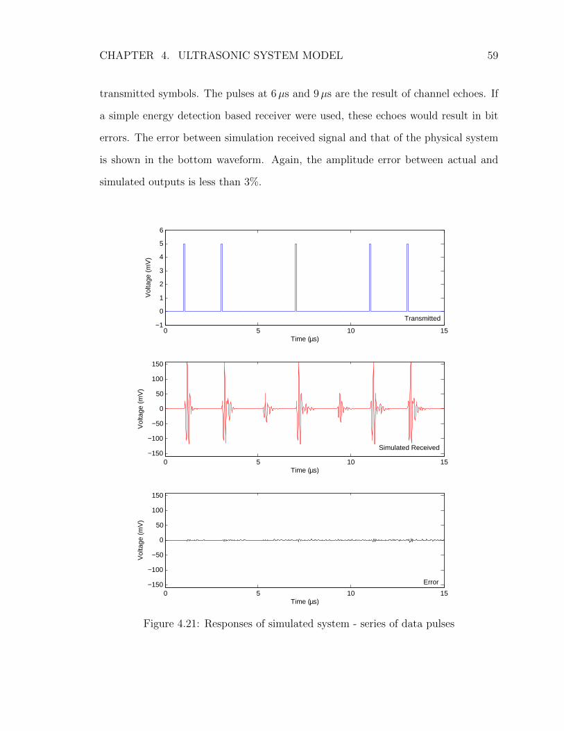
CHAPTER 4. ULTRASONIC SYSTEM MODEL 59
transmitted symbols. The pulses at 6µs and 9µs are the result of channel echoes. If
a simple energy detection based receiver were used, these echoes would result in bit
errors. The error between simulation received signal and that of the physical system
is shown in the bottom waveform. Again, the amplitude error between actual and
simulated outputs is less than 3%.
0 5 10 15−1
0
1
2
3
4
5
6
Vol
tage
(m
V)
Time (µs)
Transmitted
0 5 10 15−150
−100
−50
0
50
100
150
Vol
tage
(m
V)
Time (µs)
Simulated Received
0 5 10 15−150
−100
−50
0
50
100
150
Vol
tage
(m
V)
Time (µs)
Error
Figure 4.21: Responses of simulated system - series of data pulses

CHAPTER 4. ULTRASONIC SYSTEM MODEL 60
Response to an arbitrary waveform The final test shows the response of the
real and simulated channels to an arbitrary input waveform. The top pane of Figure
4.22 shows the transmitted waveform. The bottom pane shows the outputs form both
the physical and simulated systems, overlayed. The time axis has been expanded to
show only the primary received pulse. The exotic transmitted pulse used here may
considered the superposition of scaled, shifted versions of the “basic” pulses used in
the training algorithm. The agreement between real and simulated responses indicates
that the linear model assumption is reasonable.
0 0.1 0.2 0.3 0.4 0.5 0.6 0.7 0.8 0.9 1−6
−4
−2
0
2
4
6
Vol
tage
(V
)
Time (µs)
Transmitted
0 0.1 0.2 0.3 0.4 0.5 0.6 0.7 0.8 0.9 1−150
−100
−50
0
50
100
Vol
tage
(m
V)
Time (µs)
Received
PhysicalSimulated
Figure 4.22: Responses of physical and simulated systems - arbitrary pulse shape

CHAPTER 4. ULTRASONIC SYSTEM MODEL 61
4.5.3 Test of Channel Linearity
The channel model developed in Section 4.1 assumes that the ultrasonic channel is
linear. The tests conducted in the previous section do not contradict this hypothesis.
In this section, two additional tests are performed to the error between the response
of the physical system and that of the linear model.
Consider a system described by the operator G that maps inputs x(t) into outputs
y(t), expressed as y(t) = G(x(t)). Given any two inputs x1(t) and x2(t), and their
respective outputs y1(t) and y2(t), the system G is linear if and only if the properties
of additivity and homogeneity hold, i.e.
α1y1(t) + α2y2(t) = G(α1x1(t) + α2x2(t)).
To measure how closely the linear model matches the physical system’s response,
we begin by constructing two waveforms x1[n] and x2[n], and sending them into the
system. Figure 4.23(a) shows the input-output pair x1[n] and y1[n]. The signal x1[n]
is a 60 ns pulse with 1 volt amplitude. Figure 4.23(b) shows the input-output pair
x2[n] and y2[n]. The signal x2[n] is a 100 ns pulse with 1 V amplitude followed by a
second 100 ns pulse with -1 V amplitude. These two pulses have been chosen because
they are spectrally rich and linearly independent of one another.
The remainder of this section describes the tests that were performed to individ-
ually test for homogeneity and additivity in the channel, and the numerical results
obtained.
Homogeneity The set of input signals x[n] = αx2[n] for α ∈ [−5, ... , 5] volts was
sent through the channel and the output y[n] was recorded. For each input, the signal
y[n] = α y2[n] was generated, and the error signal e[n] = y[n] − y[n] was calculated.
Over the {-5 5} volt amplitude range of interest, the error signal’s peak amplitude was
CHAPTER 4. ULTRASONIC SYSTEM MODEL 62
0 10 20 30 40 50 60 70 80
−1
0
1
Vol
tage
(V
)
Time (µs)
Transmitted
0 10 20 30 40 50 60 70 80−1
−0.5
0
0.5
1
Vol
tage
(V
)
Time (µs)
Received
(a) Basis pulse No.1 - x1(n)
0 10 20 30 40 50 60 70 80
−1
0
1
Vol
tage
(V
)
Time (µs)
Transmitted
0 10 20 30 40 50 60 70 80−1
−0.5
0
0.5
1
Vol
tage
(V
)
Time (µs)
Received
(b) Basis pulse No.2 - x1(n)
Figure 4.23: The two basis pulses used to test channel linearity
less than 3 ns for received signals with a nominal 200 ns amplitude – an error of less
than 2%. The input signal amplitude range chose coincides with the pulse amplitudes
used during operation of the communication system. This test indicates that with the
chosen signals, homogeneity is a good working assumption for the ultrasonic channel.
Additivity The set of input signals x[n] = x1 + x2[n − δ] for δ ∈ [−400, ... , 400]
ns was sent through the channel and the output y[n] was recorded. For each input,
the signal y[n] = y1 + y2[n − δ] was generated, and the error signal e[n] = y[n] −
y[n] was calculated. In this test as well, the error signal’s peak amplitude was less
than 2% for all input signals, indicating that with these test signals additivity is
a reasonable assumption for the ultrasonic channel. Figure 4.24 shows a snapshot
of this experiment. The transmitted signal is the sum of x1[n] and x2[n − 500 ns].
The actual output from the ultrasonic channel (y[n]) and the expected output (y[n])
coincide very closely.
Taken together, the test results above indicate that the linear channel model in
Equation 4.15 matches the response of the physical system to within 2% with respect
to the test inputs chosen. As with any physical system, we cannot prove linearity from

CHAPTER 4. ULTRASONIC SYSTEM MODEL 63
0 0.5 1 1.5
−5
0
5
Vol
tage
(V)
Time (µs)
Transmitted
0 0.5 1 1.5
−2
−1
0
1
2
Time (µs)
Vol
tage
(V)
Received
ActualExpected
Figure 4.24: The sum of the two shifted basis pulses is used to test additivity
testing input-output pairs. However, linearity for the set of signals we have tested
appears to be a good working assumption.

64
5. Basic Transceiver Designs
In Chapter 2, the echo characteristics of the ultrasonic channel, and the inter-
symbol interference they cause, were introduced. Subsequently these effects were
captured with the mathematical models developed in Chapter 4. In the current chap-
ter, the design of pulse amplitude modulated (PAM) transceivers sending baseband
data will be considered, and the design issues relevant to reliable communication
with this scheme are discussed. The transceiver design techniques presented in this
chapter do not attempt to eliminate ISI (which would require the use of a channel
equalizer), but rather operate in the presence of ISI. These transceiver designs result
in low hardware/computational complexity, but intersymbol interference limits their
data throughput. In the next chapter, more advanced transceiver designs will be
considered that use various equalization techniques to suppress echoes and achieve
much higher data throughput. The high-speed operation of these transceivers comes
at the expense of higher hardware/software complexity.
Ultrasonic through-metal communication systems are finding use in a wide vari-
ety of applications. Some require high throughput, while others require low power
consumption. The motivation for developing multiple transceiver designs – ranging
from low complexity, low power to high complexity, high throughput – is so that the
best design can be matched to each application.
5.1 Communication System Model
Consider an echo free ultrasonic communication channel. When it is excited with
a narrow pulse (e.g., the 60 ns, 5 V pulse that has been used previously), the reso-
nant characteristics of the transducers produce an oscillatory output signal that can

CHAPTER 5. BASIC TRANSCEIVER DESIGNS 65
be approximated as a Gaussian pulse (see Section 4.2.2) – the product of a sinu-
soidal carrier and an Gaussian envelope. Data can be transmitted on a series of
such transmitted pulses by modulating some pulse parameter (amplitude, width, po-
sition) using the incoming data. Figure 5.1 illustrates data transmission over an ideal
(noiseless, distortionless, zero-ISI) channel using eight level pulse amplitude modu-
lation (8-PAM). For each transmitted symbol, one Gaussian pulse is received. The
amplitude of the received pulse encodes the data being transmitted. In this example,
the sequence [7 1 4 6 2] has been transmitted.
0 1 2 3 4 5 60
1
2
3
4
5
6
7
Time (µs)
8−P
AM
Sym
bol
0 1 2 3 4 5 60
1
2
3
4
5
6
7
Time (µs)
8−P
AM
Sym
bol
Transmitted signalValid symbol amplitudes
Received signal envelopeSample instantsDecisiton thresholds
Figure 5.1: PAM received over an ideal ultrasonic channel
Using M -ary PAM, all of the signal’s information content is encoded in the am-
plitude of received signal – the amplitude takes one of M values. In this chapter,
we model transmission of symbols through the ultrasonic channel as baseband PAM
transmission using Gaussian pulse shaping. Furthermore, the receiver will be incoher-

CHAPTER 5. BASIC TRANSCEIVER DESIGNS 66
ent, using an envelop detector, such that only the amplitude (and not the sign) of the
transmitted pulse can be discerned. In the next chapter, more complex transmissions
schemes will be investigated.
Figure 5.2(a) shows the equivalent channel model used to study PAM commu-
nication thought the ultrasonic channel. Incoming symbols Am are sent through a
transmitting filter/pulse shaper Gt that maps each symbol into a Gaussian pulse of
appropriate amplitude. The Gaussian pulses pass through the channel Hc, which
induces echoes. The signal emanating from the channel then passes through a receiv-
ing filter Gr. Finally, the signal passes through a detector that samples the received
signal in synchronization with the transmitted symbol rate, and maps each sample
to one of the M transmitted symbols. The output of the channel is the estimate Am
of the transmitted symbol Am.
Gt Hc
n(t)
Gr
Am x(t) y(t) x(t) Am
(a) Equivalent system model
P
n(t)
P ∗Am x(t) y(t) x(t) Am
E
(b) Physical system components
Figure 5.2: Components of the PAM communication system
Figure 5.2(b) shows how the physical components of the communication system
correspond to the model components. The ultrasonic channel’s primary path transfer

CHAPTER 5. BASIC TRANSCEIVER DESIGNS 67
function (P ) acts as a pulse shaper, mapping rectangular pulses into Gaussian pulses
of appropriate amplitude. The Gaussian pulse shape is not commonly used in PAM
applications because it does not satisfy the Nyquest criterion for zero-ISI. It is being
considered here, though, because it is the implemented naturally by the ultrasonic
transducers. The communication channel Hc corresponds to the echo path transfer
function (E). The receiving filter is matched to the Gaussian transmit filter, and
thus has the transfer function P ∗. Typically, additional filtering would be performed
at the received to equalize the channel response. This may be combined with the
matched filter, or placed in cascade. The focus of this chapter is on basic receiver
techniques that provide reliable communication without the use of equalization, so
this block is not present in the current model.
5.2 Intersymbol Interference
When Nyquest pulses are transmitted over an ideal channel, the received signal
amplitude at each sampling instant corresponds exactly to one of the M transmitted
symbol amplitudes. Graphically, these amplitude values are located midway between
the decision thresholds in Figure 5.1. In a non-ideal channel – one containing noise
and interference – these sampled values will not correspond exactly to the ideal values.
In the presence of AWGN, the optimal PAM detector is the maximum likelihood (ML)
detector (assuming all symbols are equally likely). Upon sampling the received signal
at the symbol instant, the ML detector assigns to that sample the closest valid symbol
value. Figure 5.3 illustrates transmission of the same symbol sequence that was used
in Figure 5.1, but over a channel containing ISI. The transmitted sequence [7 1 4 6 2]
would be incorrectly interpreted by the receiver as [7 1 3 6 1]. ISI has caused decision
errors in the third and fifth received symbols.
Despite the severe ISI in the ultrasonic channel, a low complexity transceiver

CHAPTER 5. BASIC TRANSCEIVER DESIGNS 68
0 1 2 3 4 5 60
1
2
3
4
5
6
7
Time (µs)
8−P
AM
Sym
bol
Ideal (zero−ISI) envelopeReceived signal envelopeSample instantsDecisiton thresholds
Figure 5.3: PAM received over non-ideal ultrasonic channel, contains ISI
may still achieve reliable communication by transmitting symbols at a rate “low
enough” that the echoes from successive symbols have decayed sufficiently that they
have negligible impact on one another. In this low noise environment, it is possible
to encode multiple bits per symbol. As the number of bits per symbol increases,
however, sensitivity to echo ISI also increases. It is therefore necessary to understand
the echo decay characteristics of the channel, and relate those to the maximum ISI
for a given symbol rate. From this, bit rate can be optimizes as a function of symbol
rate and number of bits per symbol.
The simulation results in Figure 5.4 show the interference measured at the output
of the ultrasonic channel as a function of symbol rate. The symbol rate ts is swept
from 0.4 µs to 10.0 µs. At each step, a random 100 symbol sequence is transmitted
thought the channel and the ISI level is measured at the receiver. The lowest signal-
to-ISI ratio (SIR) is reported for each time step. The channel simulation model used
here was extracted from a physical ultrasonic channel whose round trip echo period
is tr = 2.21µs, using the procedure presented in Chapter 4.
The simulation shows several interesting results. First, at multiples of the echo
round trip time (2.21 µs, 4.42 µs, 6.63 µs,...), the SIR is particularly low. Second,
the ISI varies greatly as ts varies from one multiple of tr to the next, and at specific
symbol rate SIR is very high (e.g., 40 dB at ts = 4µs). In general, the interference

CHAPTER 5. BASIC TRANSCEIVER DESIGNS 69
phenomena in the channel are difficult to describe analytically, but in the following
sections, the dependency of ISI on symbol period will be investigated, and analytical
bounds will be established to describe the worst case ISI.
0 1 2 3 4 5 6 7 8 9 100
5
10
15
20
25
30
35
40
45S
igna
l−to
−In
terf
eren
ce r
atio
(dB
)
Symbol period (µs)
Figure 5.4: The measured ISI varies significantly with symbol rate
5.3 Echo Decay Envelope
In Chapter 4, the ultrasonic channel was decomposed into a primary path and
an echo path. With respect to the communication system shown in Figure 5.2, the
primary path accounts for pulse shaping (modeled in Gt), and the echo path accounts
for ISI (modeled in Hc). The n-th symbol to be transmitted produces the baseband
pulse xn(t) at the pulse shaper output,
sm(t) = Am p(t) = m · p(t), for m ∈ {0, 1, ... , M − 1}, (5.1)
xn(t) = sm[n](t− n ts) = m[n] p(t− n ts). (5.2)
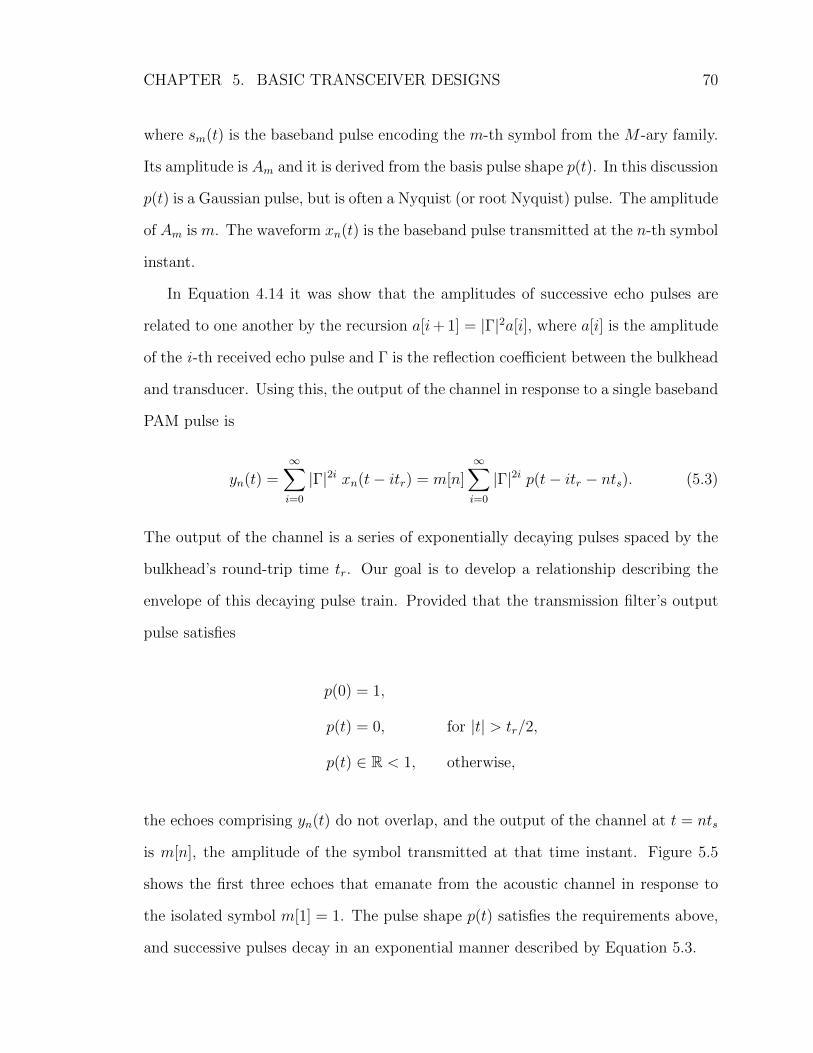
CHAPTER 5. BASIC TRANSCEIVER DESIGNS 70
where sm(t) is the baseband pulse encoding the m-th symbol from the M -ary family.
Its amplitude is Am and it is derived from the basis pulse shape p(t). In this discussion
p(t) is a Gaussian pulse, but is often a Nyquist (or root Nyquist) pulse. The amplitude
of Am is m. The waveform xn(t) is the baseband pulse transmitted at the n-th symbol
instant.
In Equation 4.14 it was show that the amplitudes of successive echo pulses are
related to one another by the recursion a[i+ 1] = |Γ|2a[i], where a[i] is the amplitude
of the i -th received echo pulse and Γ is the reflection coefficient between the bulkhead
and transducer. Using this, the output of the channel in response to a single baseband
PAM pulse is
yn(t) =∞∑i=0
|Γ|2i xn(t− itr) = m[n]∞∑i=0
|Γ|2i p(t− itr − nts). (5.3)
The output of the channel is a series of exponentially decaying pulses spaced by the
bulkhead’s round-trip time tr. Our goal is to develop a relationship describing the
envelope of this decaying pulse train. Provided that the transmission filter’s output
pulse satisfies
p(0) = 1,
p(t) = 0, for |t| > tr/2,
p(t) ∈ R < 1, otherwise,
the echoes comprising yn(t) do not overlap, and the output of the channel at t = nts
is m[n], the amplitude of the symbol transmitted at that time instant. Figure 5.5
shows the first three echoes that emanate from the acoustic channel in response to
the isolated symbol m[1] = 1. The pulse shape p(t) satisfies the requirements above,
and successive pulses decay in an exponential manner described by Equation 5.3.
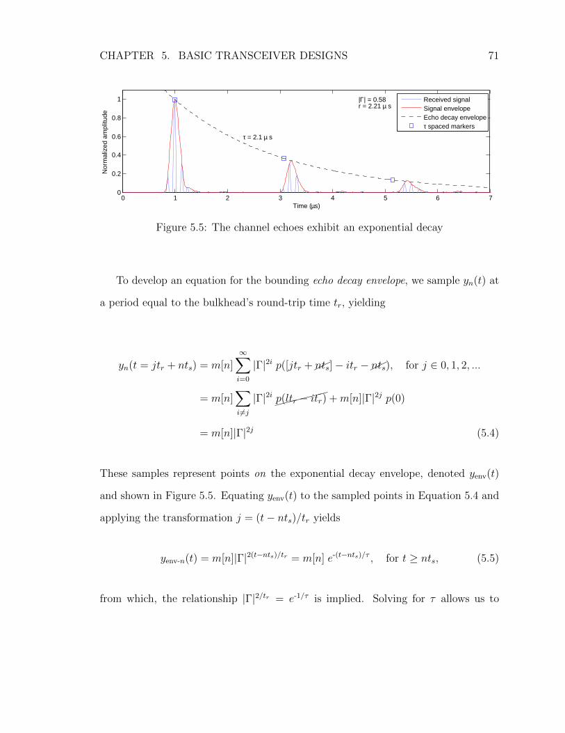
CHAPTER 5. BASIC TRANSCEIVER DESIGNS 71
0 1 2 3 4 5 6 70
0.2
0.4
0.6
0.8
1
Time (µs)
Nor
mal
ized
am
plitu
de
τ = 2.1 µ s
|Γ| = 0.58r = 2.21 µ s
Received signalSignal envelopeEcho decay envelopeτ spaced markers
Figure 5.5: The channel echoes exhibit an exponential decay
To develop an equation for the bounding echo decay envelope, we sample yn(t) at
a period equal to the bulkhead’s round-trip time tr, yielding
yn(t = jtr + nts) = m[n]∞∑i=0
|Γ|2i p([jtr +��nts]− itr −��nts), for j ∈ 0, 1, 2, ...
= m[n]∑i 6=j
|Γ|2i ������p(ltr − itr) +m[n]|Γ|2j p(0)
= m[n]|Γ|2j (5.4)
These samples represent points on the exponential decay envelope, denoted yenv(t)
and shown in Figure 5.5. Equating yenv(t) to the sampled points in Equation 5.4 and
applying the transformation j = (t− nts)/tr yields
yenv-n(t) = m[n]|Γ|2(t−nts)/tr = m[n] e-(t−nts)/τ , for t ≥ nts, (5.5)
from which, the relationship |Γ|2/tr = e-1/τ is implied. Solving for τ allows us to

CHAPTER 5. BASIC TRANSCEIVER DESIGNS 72
express the echo decay envelop as a decaying exponential in the more familiar form,
yenv-n(t) =
m[n] e-(t−nts)/τ , for t ≥ n ts
0, for t < n ts
where τ =-tr
2 ln|Γ|(5.6)
yielding the desired relationship between exponential decay envelope and the chan-
nel’s characteristics – round trip time (tr) and reflection coefficient (Γ). The exponen-
tial decay envelope shown in Figure 5.5 has a time constant of 2.1 µs. From equation
5.6, we see that the echo decay rate varies directly with bulkhead thickness and
inversely with the reflection coefficient. Under good bulkhead-transducer matching
(Γ ≈ 0), very little energy is retained in the bulkhead and echoes decay rapidly. Sim-
ilarly, as bulkhead thickness increases, the time between successive echoes increases,
and the echoes take longer to decay.
Figure 5.6 shows the effect of reflection coefficient on the decay rate of the echo
envelop. The echo decay time constant is normalized with respect to the round trip
echo time (i.e., it is expressed as τ/tr). For example, when Γ =√e-1 ≈ 0.61, the decay
0 0.1 0.2 0.3 0.4 0.5 0.6 0.7 0.8 0.9 10
1
2
3
4
5
Refelction coefficient (Γ)
Nor
mal
ized
ech
o de
cay
( τ /
r )
Figure 5.6: The echo decay time constant as a function of reflection coefficient

CHAPTER 5. BASIC TRANSCEIVER DESIGNS 73
time constant is equal to one round trip time period (τ = tr); when Γ =4√e-1 ≈ 0.78,
the decay time constant is equal to two round trip time periods (τ = 2 tr). As |Γ| → 1,
the echo train takes infinitely long to decay. In our experimentation, typical values
of Γ are in the range [0.45, 0.55], giving decay time constants of τ ∈ [ 0.63 tr, 0.84 tr ].
5.3.1 Worst Case ISI
For the ultrasonic channel having the transient response shown in Figure 5.5, the
maximum ISI induced by a symbol received at t = 0 on a symbol sampled at some
t > 0 is given by Equation 5.6. When a sequence of symbols is transmitted, the ISI
experienced at time t is the sum of the ISI components contributed by all previously
received symbols. For a sequence of symbols beginning at t = -∞ and having period
ts, the received signal sampled at time zero can be expressed in terms of the symbol
being received at time zero and the worst case ISI present at time zero due to all
previously received symbols, given in Equation 5.7.
yenv(0) =0∑
n=-∞
yenv-n(0) =0∑
n=-∞
m[n] ents/τ
= m[0] +∞∑n=1
m[-n] e-nts/τ
= m[0] + Ienv[ts,m ] (5.7)
The term Ienv[ts,m ] gives the worst case ISI that results from transmission of the
sequence m , i.e. m[-∞], ...,m[-2],m[-1], at a symbol rate ts over a channel with echo
decay constant τ . The worst case ISI is different for each transmitted sequence m ,
and we are interested in finding the sequence m that maximizes the worst case ISI.
For the PAM symbol alphabet whose normalized symbol amplitudes are uniformly
distributed between 0 and 1, the sequence m[n] = 1 for n ∈ {-∞, ..., 0} maximizes

CHAPTER 5. BASIC TRANSCEIVER DESIGNS 74
the worst case ISI.
Ienv[ts, m ] =∞∑n=0
m[-n] e-nts/τ −m[0]
=∞∑n=0
e-nts/τ − 1
=1
1− e-ts/τ− 1 (5.8)
Figure 5.7 shows the same measured signal-to-interference ratio presented earlier,
with the exponential worst case bound overlayed. As expected, the symbol rates that
are at multiples of the round trip time correspond to points on the exponential bound
curve, and give rise to especially high ISI. In general, however, the bound in Equation
5.8 underestimates the actual ISI present at particular symbol rates. Its simplicity
nonetheless makes it a convenient, closed form bound. In Section 5.5, this ISI bound
will be used to determine an upper limit on the achievable data rate in this equalizer
free communication system.
0 1 2 3 4 5 6 7 8 9 100
5
10
15
20
25
30
35
40
45
Sig
nal−
to−
Inte
rfer
ence
rat
io (
dB)
Symbol period (µs)
Masured worst case ISIExponential decay bound
Figure 5.7: The signal-to-interference bound for the exponential decay approximationcompared to the measured value

CHAPTER 5. BASIC TRANSCEIVER DESIGNS 75
5.4 Symbol/Echo Synchronization
The analysis in the previous section provided an ISI bound that approximated the
decaying pulse train phenomenon as an exponentially decaying envelope. This bound
is convenient because it is dependant only on the time constant of the echo decay,
but in general it is very conservative. The echoes found in the ultrasonic channel are
different from the ISI found in most hardwired and wireless channels in that they are
well structured – characterized by an exponentially decaying series of equally spaced
pulses. Only when the data symbols are sent at a rate equal to some multiple of the
echo period does the ISI experienced approach that predicted by Equation 5.8. By
interleaving the transmitted symbols with channel echoes, ISI can be greatly reduced,
and data rate can be increased.
The design of the communication system in this chapter has assumed the use of
a Gaussian symbol shaping filter, due to the approximately Gaussian response of the
ultrasonic transducers to a rectangular excitation pulse. While the Gaussian pulse
does not satisfy the Nyquist criterion, the pulse does decay rapidly, so in an echo free
environment, ISI from adjacent primary pulses can be controlled by proper selection
of symbol period. The illustration in Figure 5.1 shows an example where symbol
spacing is sufficient to ensure low ISI. Strictly speaking, the Gaussian pulse is infinite
duration, but in practice, some time interval tp can be found such that the pulse
shaping filter’s response is essentially zero outside of that interval.
p(0) = 1
p(t) ≈ 0, for |t| > tp/2,
p(t) ∈ R < 1, otherwise (5.9)

CHAPTER 5. BASIC TRANSCEIVER DESIGNS 76
We begin by expressing the bulkhead’s round-trip time tr and symbol period ts
as integer multiples of the time slot width, tw. Let kr denote the number of time slots
between each echo, and ks denote the number of time slots between each transmitted
symbol. If a common factor g exists between the two, it is factored out to give kr
and ks, respectively.
tr = kr tw, ts = ks tw, where kr =
⌊2 trtp
⌋(5.10)
kr = g kr, ks = g ks, where g = GCF(kr, kt) (5.11)
Due to the choice of tw, the i-th echo resulting from a pulse transmitted at time zero
is centered within the ikr-th time slot. Furthermore, the n-th symbol is transmitted
within the nks-th time slot. Since the Guassian pulse width is less than the time
slot width (tw ≥ tp), an echo only interferes with a symbol if they are centered in
the same time slot. Figure 5.8 illustrates the concept with kr = 6 and ks = 5. The
exponentially decaying pulse train from the symbol transmitted at t = 0 is spaced at
multiples of six time slots. If symbols are transmitted every five time slots, we see
that interference occurs in time slot thirty, between the sixth transmitted symbol and
the fifth echo of symbol zero.
Figure 5.9 shows the same ultrasonic channel, but now when transmitting at
a symbol rate of ks = 3. At this symbol rate, there is interference between the
second transmitted symbol and the first echo, leading to much stronger ISI than was
present in the prior example. The relationship between ks and ks dictates the way
in which symbols and echoes interact. Our goal is to develop a relationship between
the parameters ks and ks, and the worst case ISI that results. From this, we can
determine the symbol period that maximizes data rate.
These examples only illustrate the interference between a pair of symbols. In

CHAPTER 5. BASIC TRANSCEIVER DESIGNS 77
0 5 10 15 20 25 30 350
0.2
0.4
0.6
0.8
1
Time slot
Sym
bol a
mpl
itude
Echo train from first transmitted symbolSubsequent transmitted symbols
Figure 5.8: Interleaving symbols between echoes with tr = 6 tp, ts = 5 tp. Interferenceat fifth echo.
0 5 10 15 20 25 30 350
0.2
0.4
0.6
0.8
1
Time slot
Sym
bol a
mpl
itude
Echo train from first transmitted symbolSubsequent transmitted symbols
Figure 5.9: Interleaving symbols between echoes with tr = 6 tp, ts = 3 tp. Interferenceat first echo.
general, a series of data symbols will be transmitted, each yielding its own decaying
echo train. As a result, the ISI experienced by a symbol is a function of all symbols
that precede it.
5.4.1 Worst Case ISI
In Section 5.2, the equation yn(t) was developed to describe the received pulse
train that results from transmitting the symbol m[n]. The decaying pulse train was
the approximated by a bounding exponential yenv-n(t) and used to derive a simple

CHAPTER 5. BASIC TRANSCEIVER DESIGNS 78
upper bound on channel ISI. Beginning again with the equation for yn(t), a tighter
ISI bound can be formed by accounting for the “symbol-echo synchronization” effect
seen in Figure 5.8.
yn(t) = m[n]∞∑i=0
αi p(t− itr − nts), where α = |Γ|2
The received signal at any time is the superposition of the individual received
signals for all past transmitted symbols. Equation 5.12 describes the maximum am-
plitude of the channel output at t = 0 for a particular symbol sequence m . The time
indices have been written in terms of the time slot width tw, and the round trip and
symbol slot spacings kr and ks, respectively.
y(0) =0∑
n=-∞
yn(0) =0∑
n=-∞
m[n]∞∑i=0
αi p(−i tr − n tw)
=0∑
n=-∞
m[n]∞∑i=0
αi p(−i kr tp − n ks tw)
=∞∑n=0
m[-n]∞∑i=0
αi p([ks n− kr i] tw) (5.12)
Since the quantity [ks n − kr i] assumes only integer values, the non-overlap con-
straint of Equation 5.9 means that p([ks n − kr i] tp) is non-zero only for [ks n − kr i] =
0, or equivalently for integer values of i = n·ks/kr. The integer values of this equation
occur only at values of n = kr j for j ∈ Z. Upon substituting n = kr j and i = ks j,
Equation 5.12 can be rewritten as
y(0) =∞∑j=0
m[-kr j] αks j p(0) =
∞∑j=0
m[-kr j] αks j
= m[0] +∞∑j=1
m[-kr j] αks j
= m[0] + I[ks,m ] (5.13)

CHAPTER 5. BASIC TRANSCEIVER DESIGNS 79
Returning to the example in Figure 5.8, with kr = 6 and ks = 5, Equation 5.13 says
that the amplitude of the channel output sampled at t = 0 is
y(0) = m[0] +m[-6]α5 +m[-12]α10 +m[-18]α15 + · · ·.
For the example in Figure 5.9, kr = 6 and ks = 3. Upon factoring out the common
factor 3 from each, we have kr = 2 and ks = 1. The channel output at t = 0 is
y(0) = m[0] +m[-2]α1 +m[-4]α2 +m[-6]α3 + · · ·.
The first term in each summation represents the desired information symbol, m[0],
and the remaining terms represent intersymbol interference. In the first example, the
ISI terms die with α5n, while in the second, they die with αn. In an M -level PAM
system, normalized symbol amplitudes take values in the range [0 1]. The worst case
ISI results when the infinite symbol sequence m[n] = 1, for n ∈ [-∞ 0], is transmitted.
The worst case ISI at t = 0 can then be expressed as
I[ks, m] =∞∑j=1
m[-kr j] αks j −m[0]
=∞∑j=1
αks j − 1
=1
1− αks j− 1 (5.14)
Equation 5.14 defines the symbol-echo synchronous ISI bound. It is interesting
to compare the maximum ISI given by this equation to the maximum ISI predicted
using the exponential decay envelope ISI bound. Upon expressing Equation 5.14 in
terms of the continuous time variable ts and expressing 5.8 in terms of α = |Γ|2, we

CHAPTER 5. BASIC TRANSCEIVER DESIGNS 80
have
I[ts, m] =∞∑j=0
αkr ts j/tr − 1 =1
1− αkr ts/tr− 1 (5.15)
Ienv[ts, m] =∞∑n=0
αts n/tr − 1 =1
1− αts/tr− 1. (5.16)
Comparison of the two equations reveals that the ISI predicted by Equation 5.15 is
less than or equal to that given by Equation 5.16, and that the two ISI bounds are
equal only when symbols are transmitted at some integer multiple of the echo round
trip time (i.e., ts = n tr for n ∈ Z+), for which kr = 1.
Figure 5.7 compares the measured channel signal-to-interference ratio with that
predicted from the bounds in Equations 5.15 and 5.16. In this example, echoes are
spaced by two time slots (i.e., kr = 2), with each time slot tw = 1.11 µs. The symbol-
echo synchronous bound is only valid for symbol periods of ts = n tw for n ∈ Z+.
Again, we note that the two bounds are equal when ts = n tr = 2n tw for n ∈ Z+.
When a symbol is transmitted in an intermediate time slot (one that is not a multiple
of tr), lower ISI levels can be realized.
In most wireless communication channels, interference is characterized as a ran-
dom process. The structured nature of echoes in the ultrasonic channel allows us to
treat them as deterministic, using one of the bounds established above. With this
knowledge, we can then find bounds on the data rate supported by the ultrasonic
channel based on desired bit-error rate.
5.5 Achievable Data Rate
The data rate supported by the ultrasonic channel is limited by two quantities,
inter-symbol interference, and channel noise. To this point, we have only considered
the former. In this section, the limiting effects of both quantities are considered, and

CHAPTER 5. BASIC TRANSCEIVER DESIGNS 81
0 1 2 3 4 5 6 7 8 9 100
5
10
15
20
25
30
35
40
45
50
Sig
nal−
to−
Inte
rfer
ence
rat
io (
dB)
Symbol period (µs)
Masured worst case ISIExponential decay boundSymbol−Echo sync bound
Figure 5.10: The ISI bound when considering symbol-echo synchronization
an optimization problem is formed to describe the achievable data rate as a function
of reflection coefficient (which controls ISI) and signal-to-noise ratio.
5.5.1 PAM Error Rate in Ideal AWGN Channel
The M -ary PAM communication scheme transmits k = log2M bits of information
per symbol, encoded in one of M waveforms. These waveforms are expressed as
sm(t) = Am p(t) = m · p(t), for m ∈ {0, 1, ... , M − 1}. (5.17)
All symbol waveforms are of identical shape, and the amplitude of the m-th waveform
is Am. The energy of p(t), denoted Ep, is
Ep =
∫ ∞−∞|p(t)|2dt. (5.18)
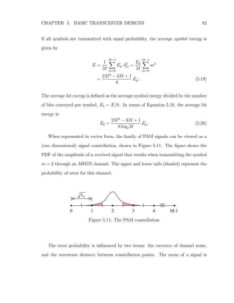
CHAPTER 5. BASIC TRANSCEIVER DESIGNS 82
If all symbols are transmitted with equal probability, the average symbol energy is
given by
E =1
M
M−1∑m=0
EpA2m =
EpM
M−1∑m=0
m2
=2M2 − 3M + 1
6Ep. (5.19)
The average bit energy is defined as the average symbol energy divided by the number
of bits conveyed per symbol, Eb = E/k. In terms of Equation 5.19, the average bit
energy is
Eb =2M2 − 3M + 1
6 log2MEp. (5.20)
When represented in vector form, the family of PAM signals can be viewed as a
(one dimensional) signal constellation, shown in Figure 5.11. The figure shows the
PDF of the amplitude of a received signal that results when transmitting the symbol
m = 2 through an AWGN channel. The upper and lower tails (shaded) represent the
probability of error for this channel.
0 1 2 3 4 M-1
pE
Figure 5.11: The PAM constellation
The error probability is influenced by two terms: the variance of channel noise,
and the minimum distance between constellation points. The norm of a signal is

CHAPTER 5. BASIC TRANSCEIVER DESIGNS 83
given by
||s(t)|| =(∫ ∞−∞|s(t)|2 dt
)1/2
,
and the distance between two symbols is ||si(t) − sj(t)||. The minimum distance
between constellation points is simply the distance between any two adjacent symbol
waveforms.
dmin = ||si+1(t)− si(t)||
=
(∫ ∞−∞|si+1(t)− si(t)|2 dt
)1/2
=
(∫ ∞−∞|[i+ 1] · p(t)− i · p(t)|2 dt
)1/2
=
(∫ ∞−∞|p(t)|2 dt
)1/2
=√Ep (5.21)
Upon substituting Equation 5.20, dmin can be expressed in terms of Eb.
dmin =
√6 log2M
2M2 − 3M + 1Eb (5.22)
It can be shown [18] that the error probability of PAM signaling is expressed in
terms of the minimum constellation distance and noise variance through Equation
5.23. Upon substituting for dmin, the error probability using unipolar PAM signaling
can be expressed in terms of SNR (Equation 5.24) or SNR per bit (Equation 5.25).
Pe = 2
(1− 1
M
)Q
(dmin√2N0
)(5.23)
= 2
(1− 1
M
)Q
(√3
2M2 − 3M + 1
E
N0
)(5.24)
= 2
(1− 1
M
)Q
(√3 log2M
2M2 − 3M + 1
EbN0
)(5.25)

CHAPTER 5. BASIC TRANSCEIVER DESIGNS 84
Figure 5.12 shows the symbol error performance of the signaling scheme for several
values of M . The graph shows that for our system – with typical SNR in the 30− 35
dB range – 16-ary PAM can be used to achieve a symbol error rate of approximately
10−5.
5 10 15 20 25 30 35 40 45 5010
−10
10−8
10−6
10−4
10−2
M=2 M=4 M=8 M=16 M=32 M=64
Sym
bol e
rror
rat
e, P
e
SNR, E/N0 (dB)
Figure 5.12: Bit error rate for unipolar PAM signaling
5.5.2 PAM Error Rate in Noisy ISI Channel
In the previous section, only the effects of noise were considered in deriving the
symbol error rate for our signaling scheme. With the assumption of zero ISI, the
derived error probability (Equation 5.25) was independent of symbol rate. When
transmitting at very low symbol rates, the zero-ISI assumption is valid, but at high
symbol rates, ISI must be considered when deriving channel error probability.
Figure 5.13 illustrates the effect of ISI using the exponential decay envelope bound
if Equation 5.16. When symbols are transmitted at a rate equal to the echo decay
time constant (ts = τ), the worst case ISI is Ienv(τ, s) = 0.58. Consider 2-level PAM

CHAPTER 5. BASIC TRANSCEIVER DESIGNS 85
transmission, with transmitted symbols having amplitudes of Am ∈ {0, 1}. A decision
error occurs when ISI causes the received symbol’s amplitude to cross the detector’s
decision threshold of 0.5, which can happen only if I > 0.1. Clearly, the ISI present
at this symbol rate can induce decision errors with 2-PAM transmission.
0 0.2 0.4 0.6 0.8 1 1.2 1.4 1.6 1.8 20
0.5
1
1.5
2
Nor
mal
ized
sym
bol a
mpl
itude
Symbol period normalized to echo time constant (ts/τ)
Echo envelopes of individual symbolsWorst case received sigal amplitude
Figure 5.13: Worst case ISI when transmitting at symbol rate ts = τ
Next, consider symbols transmitted at a rate of ts = 4τ , shown in Figure 5.14. The
maximum ISI possible here is Ienv(4τ, s) = 0.02. At this low symbol rate, maximum
ISI amplitude is quite small. In this section, we seek to develop a relationship that
describes symbol error rate in terms of SNR and worst case ISI, or alternatively SNR
and symbol rate.
Figure 5.15 shows the PAM constellation with shaded regions corresponding to
the worst case ISI centered on each symbol value. Let dfs denote the full-scale symbol
amplitude used by the system. In terms of the minimum symbol distance (dmin given
in Equation 5.22), the full scale symbol amplitude is dfs = (M − 1) dmin, as indicated
in the figure. The worst case ISI equations given in Equations 5.15 and 5.16 describe
ISI normalized to the full-scale symbol amplitude. The actual worst case ISI amplitude

CHAPTER 5. BASIC TRANSCEIVER DESIGNS 86
0 1 2 3 4 5 6 7 80
0.2
0.4
0.6
0.8
1
1.2
1.4
Nor
mal
ized
sym
bol a
mpl
itude
Symbol period normalized to echo time constant (ts/τ)
Echo envelopes of individual symbolsWorst case received sigal amplitude
Figure 5.14: Worst case ISI when transmitting at symbol rate ts = 4τ
for a given symbol rate is given by
I = dfs I = (M − 1) dmin I (5.26)
= (M − 1)√Ep I . (5.27)
0 1 2 M-1
mind I~
2
minfs dMd )1(
mind~
Figure 5.15: The PAM constellation showing ISI bounds
The presence of ISI reduces the effective distance between symbols. In an eye
diagram, this is manifest as a closure of the eye in the vicinity of the sampling instant.
For a given symbol distance dmin, an effective distance dmin can be expressed in terms

CHAPTER 5. BASIC TRANSCEIVER DESIGNS 87
of the ISI level.
dmin = dmin − 2 I
=√Ep − 2 I (M − 1)
√Ep
= [1− 2 I (M − 1)]√Ep
= β√Ep, where β = 1− 2 I (M − 1) (5.28)
The effective minimum distance is just dmin multiplied by some constant β ≤ 1. Note
that β = 1 only when no ISI is present, and can take negative values for high ISI
or when the alphabet consists of a large number of symbols. A negative value of β
indicates that worst case ISI will lead to (ISI induced) symbol errors. The symbol
error probability can now be expressed in terms of both noise and ISI. The multiplier
β inside the Q-function causes the bit error rate curve to shift to the right with
increasing ISI level.
Pe = 2
(1− 1
M
)Q
(dmin√2N0
)
= 2
(1− 1
M
)Q
(β
√3
2M2 − 3M + 1
E
N0
)(5.29)
= 2
(1− 1
M
)Q
(β
√3 log2M
2M2 − 3M + 1
EbN0
)(5.30)
Figure 5.16 shows two sets of curves generated for different ISI levels. Figure
5.16(a) shows that when the ISI level is 10%, only 2-ary and 4-ary PAM communi-
cation are supported by the channel. The ISI-free 4-ary BER curve is also shown.
To maintain the error performance realized in the ISI-free channel using 4-PAM, an
SNR increase of 8 dB is required. Figure 5.16(b) shows the effect of a 1% ISI level.

CHAPTER 5. BASIC TRANSCEIVER DESIGNS 88
Alphabet sizes of up to M = 32 are supported. The SNR degradation here is signif-
icantly less; a 1 dB SNR increase is required to maintain the 4-PAM ISI-free BER
performance.
5 10 15 20 25 30 35 40 45 5010−10
10−8
10−6
10−4
10−2
M=2 M=4
Sym
bol e
rror
rate
, Pe
SNR, E/N0 (dB)
(a) 10% ISI amplitude
5 10 15 20 25 30 35 40 45 5010
−10
10−8
10−6
10−4
10−2
M=2 M=4 M=8 M=16
Sym
bol e
rror
rat
e, P
e
SNR, E/N0 (dB)
(b) 1% ISI amplitude
Figure 5.16: Bit error rate degradation with increase in ISI level. ISI free M = 4curve shown also.
5.5.3 Data Rate Optimization
The raw data rate through the ultrasonic channel is the product of the symbol
rate (fs = 1/ts) and the number of bits conveyed per symbol (k).
R = k/ts = k fs where k = log2M (5.31)
We have shown that as symbol rate increases, ISI also increases. We have also shown
that the severity of ISI limits the size of the PAM alphabet (and therefore the size of
k) that can be used. In this section, a systematic approach is presented to determine
the optimal symbol rate (and resulting data rate) for the ultrasonic channel. The
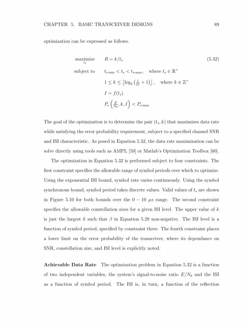
CHAPTER 5. BASIC TRANSCEIVER DESIGNS 89
optimization can be expressed as follows.
maximizets
R = k/ts (5.32)
subject to ts-min < ts < ts-max, where ts ∈ R+
1 ≤ k ≤⌊log2
(12I
+ 1)⌋, where k ∈ Z+
I = f(ts)
Pe
(EN0, k, I
)< Pe-max
The goal of the optimization is to determine the pair (ts, k) that maximizes data rate
while satisfying the error probability requirement, subject to a specified channel SNR
and ISI characteristic. As posed in Equation 5.32, the data rate maximization can be
solve directly using tools such as AMPL [59] or Matlab’s Optimization Toolbox [60].
The optimization in Equation 5.32 is performed subject to four constraints. The
first constraint specifies the allowable range of symbol periods over which to optimize.
Using the exponential ISI bound, symbol rate varies continuously. Using the symbol
synchronous bound, symbol period takes discrete values. Valid values of ts are shown
in Figure 5.10 for both bounds over the 0 − 10 µs range. The second constraint
specifies the allowable constellation sizes for a given ISI level. The upper value of k
is just the largest k such that β in Equation 5.28 non-negative. The ISI level is a
function of symbol period, specified by constraint three. The fourth constraint places
a lower limit on the error probability of the transceiver, where its dependance on
SNR, constellation size, and ISI level is explicitly noted.
Achievable Data Rate The optimization problem in Equation 5.32 is a function
of two independent variables, the system’s signal-to-noise ratio E/N0 and the ISI
as a function of symbol period. The ISI is, in turn, a function of the reflection

CHAPTER 5. BASIC TRANSCEIVER DESIGNS 90
coefficient. As E/N0 increases, so to does achievable bit rate. As Γ decreases, echo
decay rate increases, and bit rate increases. Here, we look at the effect of each of
these parameters individually on the maximum achievable channel bitrate. We use
unipolar PAM signaling and a maximum error probability of 10-5.
Effect of Signal-to-Noise Ratio First, the reflection coefficient is fixed at Γ =
0.48 and the E/N0 is varied over the range 10− 50 dB. For each (E/N0,Γ) pair, the
optimization in Equation 5.32 is carried out to yield the pair (ts, k) that maximizes
data rate. Figure 6.6 shows the minimum achievable data rate as a function of signal-
to-noise ratio using both the exponential and synchronous ISI bounds (Equations
5.15 and 5.16 , respectively). As expected, the more conservative exponential bound
predicts a lower achievable data rate than the synchronous bound.
10 15 20 25 30 35 40 45 500
500
1000
1500
2000
2500
Signal−to−Noise Ratio, E/N0 (Γ fixed at 0.48)
Max
bit
rate
(kb
ps)
k = 2 bits/sym,fs = 286k sym/sec
k = 1 bits/sym,fs = 1339k sym/sec
Synchronous boundExponential bound
Figure 5.17: Bit rate as a function of SNR with Γ fixed at 0.48
According to the exponential bound, at a 30 dB SNR, the minimum achievable

CHAPTER 5. BASIC TRANSCEIVER DESIGNS 91
bit rate is 572 kbps (2 bits/sym · 286 ksym/sec). The synchronous bound indicates
a minimum bit rate of 1.34 Mbps (1 bit/sym · 1.34 M-sym/sec) at the same SNR.
Effect of Reflection Coefficient Next, E/N0 is fixed at 30 dB and the reflection
coefficient is varied over the range 0.20 − 0.80. Figure 5.18 shows the minimum
achievable data rate as a function of reflection coefficient, again using the exponential
and synchronous ISI bounds. As expected, better transducer-bulkhead matching
(smaller Γ) results in lower echo amplitude and higher achievable data rate. The
same operating point shown in Figure 6.6 (Γ = 0.48, E/N0 = 30 dB) is shown on this
graph as well, and indicates the same achievable bit rate.
0.2 0.3 0.4 0.5 0.6 0.7 0.80
500
1000
1500
2000
2500
3000
Reflection coefficient, Γ (E/N0 fixed at 30 dB)
Max
bit
rate
(kb
ps)
Synchronous boundExponential bound
Figure 5.18: Bit rate as a function of Γ with SNR fixed at 30 dB
Simulation Results The results in Figure 6.6 indicate that a data rate of 1.4 Mbps
can be achieved at a bit-error rate of 10−5 when ts and k are chosen properly. This can

CHAPTER 5. BASIC TRANSCEIVER DESIGNS 92
be verified using the channel simulation model with the aid of an eye diagram. Figure
5.19(a) shows the eye diagram generated by sending 200 random symbols thought the
channel for ts = 0.75µs and k = 1 bit. The interference results in some closure of the
eye, but the remaining noise margin is sufficient to meet the BER requirement. Figure
5.19(b), on the other hand, shows the same symbol rate, but for k = 2 bits/sym. Here,
the eye is completely closed, indicating that symbol errors will occur. Note that the
data in Figure 6.6 also indicates that this (ts k) pair is not supported.
−100 −80 −60 −40 −20 0 20 40 60 80 1000
0.2
0.4
0.6
0.8
1
Time realtive to sample instant (ns)
Am
plitu
de
(a) k = 1 bit/symbol, eye open
−100 −80 −60 −40 −20 0 20 40 60 80 1000
0.2
0.4
0.6
0.8
1
Time realtive to sample instant (ns)
Am
plitu
de
(b) k = 2 bits/symbol, eye closed
Figure 5.19: Eye diagrams of PAM transmission at fs = 1338k symbols/sec
5.6 Summary
In this chapter, techniques for designing reliable equalizer-free communication
transceivers were presented. It is obvious that transmitting at a “low enough” sym-
bol rate will mitigate the effects of echo induced ISI, and in this chapter we have
provided numerical bounds to quantify this symbol rate. The motivation for con-
sidering such simple transceiver designs is that they translate into simple, low-cost,

CHAPTER 5. BASIC TRANSCEIVER DESIGNS 93
low-power hardware implementations, making them ideal for battery powered or en-
ergy harvesting based systems.
The data rate in the presence of echoing was determined by first deriving bounds
on the echo ISI as a function of symbol rate. The exponential bound requires knowl-
edge only of the reflection coefficient between transducer and bulkhead. The syn-
chronous bound requires determination of reflection coefficient, echo period, and pulse
width, so its implementation is more difficult in practice. Furthermore, this method
requires that the symbol rate can be precisely adjusted (to achieve synchronization
with the echo period).
While the methods presented in this chapter represent a very simple set of transceivers,
they should be considered in applications that require low data rates. In the following
chapter, more complex equalizer-based designs will be developed for high data rate
applications.

94
6. Advanced Transceiver Designs
The goal of the previous chapter was to present transceiver designs that resulted in
very simple hardware/software implementations. Those designs simply avoided echo
related intersymbol interference by transmitting at a sufficiently low data rate, or by
interleaving transmitted symbols with echo pulses in a way that reduces the effective
channel interference. While those techniques are ideal for low power, low bandwidth
applications, the presence of ISI limits the channel bandwidth to a point well below
the theoretical limit. Intersymbol interference in high-speed communication channels
is traditionally addressed through the used of channel equalizers. In this chapter, sev-
eral common equalization techniques are applied to ultrasonic transceiver design. In
addition, we derive an equalizer based on the channel model developed in Chapter 4.
The penalty paid for all of the techniques presented in this chapter is increased tran-
sceiver cost and complexity, but in applications where high data rates are required,
this may be justified. The experimental and simulation results presented throughout
this chapter were performed using the test setup presented Chapter 2 and channel
model developed in Chapter 4.
6.1 Channel Model Based Equalizer
In Chapter 4, a block diagram of the ultrasonic channel (reproduced in Figure 6.1)
was formed that decomposed the channel into a primary path and an echo path.
It was shown that the primary path transfer function acts as a pulse shaper, and
the echo path transfer function accounts for acoustic energy being reflected within
the bulkhead. Once an estimate of the channel model is formed, it can be used to
construct a simple equalizer. We begin by considering an equalizer that, when placed

CHAPTER 6. ADVANCED TRANSCEIVER DESIGNS 95
Px y
E
+
Figure 6.1: Ultrasonic channel model developed in Chapter 4
in cascade with the ultrasonic channel, causes complete cancelation of the echo portion
of the channel response. In terms of the transfer functions of the equalizer (He) and
the channel (Hc), the overall system transfer function (H) is
H = HeHc = P.
In other words, the transfer function of the composite system reduces to the transfer
function of the primary path. Using Equation 4.3, the equalization filter that exactly
cancels the channel echoes is given by
He =P
Hc
= 1− E, (6.1)
which depends only on the echo transfer function, E. The block diagram of Figure 6.2
shows the interconnection of equalizing filter and channel. E denotes the estimate of
the actual echo transfer function E. Two approximations will be considered to form
the model of E, each of differing complexity and effectiveness. The simplified echo
path model assumes that E is an attenuator in cascade with an ideal delay element,
i.e., the echoes that emanate from the channel are scaled, time delayed version of
one another. The improved echo path model, on the other hand, models the disper-
sive effects of the channel in addition to the attenuation and delay characteristics.
This model yields a superior equalization filter at the expense of greater transceiver

CHAPTER 6. ADVANCED TRANSCEIVER DESIGNS 96
complexity.
Px y
E
+
E
−
Figure 6.2: Construction of the predistortion filter
The echo transfer function, E, accounts for several phenomena experienced as an
acoustic signal makes a single round trip through the bulkhead. A signal within the
bulkhead, incident upon the receiving side, meets an impedance mismatch between
the bulkhead wall and the receiving transducer. A portion of the energy is coupled to
the transducer (appearing as a voltage at the output) and the remainder of the energy
is reflected back within the bulkhead toward the transmitting transducer. As the
signal travels through the bulkhead material, it is attenuated and dispersed. When
the signal reaches the other bulkhead wall, it meets another impedance mismatch
and again, a portion of the energy is coupled to the transducer while the remainder
is reflected back toward the reverer side. This process continues until all acoustic
energy is dissipated within the bulkhead or transducers.
As described, the bulkhead can be considered a cascade of several subsystems. In
this analysis, we represent all of the effects described above by a cascade of an ideal
delay and a rational transfer function. The delay element accounts for the round
trip delay of acoustic signals, and the transfer function provides a lumped element
approximation of all other magnitude and phase characteristics. The filter will be
implemented in a digital signal processor, so we have chosen to describe it in discrete
time form.

CHAPTER 6. ADVANCED TRANSCEIVER DESIGNS 97
E(z) = El(z)z−r
He(z) = 1− El(z)z-r (6.2)
where z−r denotes the round trip delay of acoustic signals (in samples) and El(z)
is the lumped element approximation of all other bulkhead effects. The remainder
of this section discusses methods of building the equalizer from experimental data.
Two equalizers are presented, based on two models of the echo transfer function of
differing complexity and accuracy.
6.1.1 Simplified Echo Path Model
We begin by assuming that the echos in the ultrasonic channel are characterized
by an exponentially decaying pulse train, i.e. successive echoes are equally spaced
and differ in amplitude by a factor α. Under this assumption, Equation 6.2 reduces
to
He(z) = 1− α z-r, (6.3)
requiring the estimation of two parameters, the decay constant α and the round trip
echo delay r. A block diagram of the equalizer is shown in Figure 6.5. In the previous
chapters, we have discussed the estimation of both the decay constant and round
trip time. Figure 6.3 shows the effect of an equalizer derived from the basic channel
model. Here, we assume that the equalizer is placed on the transmitting side of the
channel, but it works identically when placed at the receiver side. The first curve in
the figure shows that the equalizer’s effect is to augment each transmitted pulse with a
cancelation pulse whose time offset and amplitude correspond to the echo period and
decay constant of channel echoes. The second curve shows the received signal that

CHAPTER 6. ADVANCED TRANSCEIVER DESIGNS 98
results when no equalization is used, while the third curve shows the channel output
when equalization is used. The effect of the cancelation pulse to cause destructive
interference with and reduce the amplitude of channel echoes.
0 1 2 3 4 5 6 7−1
−0.5
0
0.5
1
Received with no equalization
Time (µs)
Am
plitu
de
0 1 2 3 4 5 6 7−0.5
0
0.5
1
Excitation pulse from "basic" equalizer
Time (µs)
Am
plitu
de
0 1 2 3 4 5 6 7−1
−0.5
0
0.5
1
Received with basic equalization
Time (µs)
Am
plitu
de
Figure 6.3: Echo suppression using equalizer derived from simplified channel model
The results of this experiment show that a residual echo is still present in the
received signal. This is not surprising given the simplifying assumption made about
the nature of channel echoes. Recall that the model developed in Chapter 4 treated
El(z) as a rational transfer function, where here we assume that it is a constant.
Testing this technique on several bulkheads of varying thickness has shown that it
typically results in an 8−10 dB reduction in echo energy over the unequalized channel.
The results in Figure 6.3 yield a reduction in echo energy of 9 dB.
In Chapter 5, a simulation of the channel’s signal-to-interference ratio as a function

CHAPTER 6. ADVANCED TRANSCEIVER DESIGNS 99
of symbol period was performed. Figure 6.4 shows these results along with results
from the same test performed on the equalized channel. Comparing Figures 6.4(a) and
6.4(b), we see that the equalizer effectively shifts the curve up by 9 dB, corresponding
the the 9 dB of echo energy suppression noted in Figure 6.3.
0 1 2 3 4 5 6 7 8 9 1010
15
20
25
30
35
40
45
50
SIN
R (
dB)
Symbol period (µs)
(a) Without equalization
0 1 2 3 4 5 6 7 8 9 1010
15
20
25
30
35
40
45
50
SIN
R (
dB)
Symbol period (µs)
(b) Using “simple” equalizer
Figure 6.4: SINR improvement of 9 dB realized with simplified equalizer
The simplified channel model results in an equally simple equalizer structure,
shown in Figure 6.5. The hardware implementation requires a digital delay line of
length d and one multiplication per output sample, and the equalizer can be placed on
either side of the channel. While the equalizer is less effective than alternatives dis-
cussed later in the chapter, the particularly simple implementation makes it suitable
for hardware constrained systems.
Achievable Data Rate In Chapter 5, equations were developed to related the
transmitted symbol rate to worst-case ISI amplitude in the ultrasonic channel. The
function of the simplified equalizer is to cause destructive interference in the channel

CHAPTER 6. ADVANCED TRANSCEIVER DESIGNS 100
x
α z−d
−
Figure 6.5: The implementation of the simplified equalizer
echoes. Effectively, the amplitude of the first echo is decreased, and all subsequent
echoes decay with the same decay constant seen in the equalizer-free system. The
ISI equations developed previously can be easily adapted to account for the effect of
echo cancelation. The modified equations can then be used to determine the bitrates
achievable using cancelation. The modified synchronous ISI bound, for example, is
given by
Ieq[ts, m] =1
1− βαkr ts/tr− 1, (6.4)
where β is the echo scaling factor, the ratio of echo amplitude with cancelation to its
amplitude when no cancelation is used. For example, β = 0.5 results in an equalized
echo that is one half its original value. The echo suppression achieved in Figure 6.5
yield β ≈ 0.35.
The bitrate optimization (Equation 5.32) can now be performed with this new re-
lationship for channel ISI. Figure 6.6 shows the result of performing this optimization
over the range E/N0 ∈ [10 50] dB, using the bound in Equation 6.4 and Γ = 0.48.
The results from the prior chapter, where no equalization is used, are shown for
comparison. Under channel conditions identical to those examined in the previous
chapter, the simplified equalizer provides a doubling in data rate at E/N0 = 30 dB.
While the symbol period for the two strategies is the same (0.75µs, corresponding to
transmission of one symbol during each time slot in Figure 5.8), the equalizer sup-
presses echoes sufficiently to allow the used of 4-PAM, encoding two bits per symbol.

CHAPTER 6. ADVANCED TRANSCEIVER DESIGNS 101
10 15 20 25 30 35 40 45 500
500
1000
1500
2000
2500
3000
Signal−to−Noise Ratio, E/N0 (Γ fixed at 0.48)
Max
bit
rate
(kb
ps)
k = 2 bits/sym,fs = 1339k sym/sec
k = 1 bits/sym,fs = 1339k sym/sec
With simplified equalizerWithout equalizer
Figure 6.6: Bit rate as a function of SNR with Γ fixed at 0.48
The resulting minimum bitrate is 2.68 Mbps.
The eye diagrams in Figure 6.7 show transmission through the ultrasonic chan-
nel without equalization (Figure 6.7(a)) and with equalization (Figure 6.7(b)) for
fs = 1339 ksym/sec and k = 2 bits/sym, the operating point indicated in Figure 6.6.
Without equalization, 4-ary PAM communication is not possible, but using the sim-
plified equalizer allow communication at 2.68 Mbps with a BER < 10−5
6.1.2 Improved Echo Path Model
In Chapter 4, the echo path of the channel was modeled as the cascade of a delay
element and a discrete time rational transfer function. Once this echo path model is
estimated, it can be used directly to form the equalizer given in Equation 6.2. The
equalizer’s block diagram is shown in Figure 6.8. Note that when El(z) = α, the
equalizer of Equation 6.3 is recovered.
Based on the channel model developed in Chapter 4, the hardware implementa-
tion of this equalizer requires two components, a delay line if length d samples, and

CHAPTER 6. ADVANCED TRANSCEIVER DESIGNS 102
−100 −80 −60 −40 −20 0 20 40 60 80 1000
0.2
0.4
0.6
0.8
1
Time realtive to sample instant (ns)
Am
plitu
de
(a) Without equalization
−100 −80 −60 −40 −20 0 20 40 60 80 1000
0.2
0.4
0.6
0.8
1
Time realtive to sample instant (ns)
Am
plitu
de
(b) With simplified equalizer
Figure 6.7: Eye diagrams of 4-ary PAM at fs = 1339k symbols/sec
x
El(z) z−d
−
Figure 6.8: The implementation of the advanced equalizer
an IIR filter with numerator order of three and denominator order of two (see Sec-
tion 4.4.4 for a discussion of model order estimation). This particular filter requires
five multiply-accumulate operations per output sample. Figure 6.9 shows the effect
of the improved equalizer when it is placed on the transmitter side of the channel.
Each transmitted symbol pulse is paired with a cancelation pulse, but unlike the
previous cancelation pules, this has no resemblance to the symbol pulse. This can-
celation pulse, resulting from passing the symbol pulse through the improved E(z),
causes almost complete cancelation of echoes. What echo energy remains is below
the channel’s noise amplitude.

CHAPTER 6. ADVANCED TRANSCEIVER DESIGNS 103
0 1 2 3 4 5 6 7−1
−0.5
0
0.5
1
Received with no equalization
Time (µs)
Am
plitu
de
0 1 2 3 4 5 6 7−0.5
0
0.5
1
Excitation pulse from "advanced" equalizer
Time (µs)
Am
plitu
de
0 1 2 3 4 5 6 7−1
−0.5
0
0.5
1
Received with basic equalization
Time (µs)
Am
plitu
de
Figure 6.9: Echo suppression using equalizer derived from improved channel model
Achievable Data Rate The improved equalizer effectively eliminates all echo in-
duced ISI, leaving only the channel’s bandwidth and noise to limit the achievable
data rate. In Section 5.5.1, bit error rate curves were derived for the PAM signaling
scheme using several alphabet sizes. If a symbol error rate bound of BER < 10−5
is imposed on a channel with 30 dB SNR, for example, Figure 5.12 shows that 8-
PAM (3 bits/symbol) is the largest alphabet size that can be supported. If Nyquest
pulses were being transmitted over the channel, the transmission symbol rate would
be obvious. Since we are using the naturally occurring Gaussian response as our
baseband pulse shape, however, the pulse width must be approximated. The 99%
pulse width for the prototype system (i.e., the time period containing 99% of the
pulse energy) is tpw = 1000 ns. The minimum symbol rate at which no ISI occurs is
then ts−min = tpw/2 = 500 ns. When the improved equalizer is used, the maximum

CHAPTER 6. ADVANCED TRANSCEIVER DESIGNS 104
bit rate is
R = 3 bits/500 ns = 6.00 Mbps. (6.5)
Note that this rate is dependant only on the channel SNR and bandwidth, not the
ISI or reflection coefficient of the channel. Figure 6.10 shows the eye diagram when
transmitting 8-PAM at a 500 ns period. The improved equalizer provides seven-fold
increase in data rate over the equalizer free transceiver and better than a three-fold
increase over the simplified equalizer.
−300 −200 −100 0 100 200 3000
0.2
0.4
0.6
0.8
1
Time realtive to sample instant (ns)
Am
plitu
de
Figure 6.10: PAM eye diagram when using improved equalizer
6.2 Linear Equalizer
Linear equalizers are commonly used in communication systems to combat chan-
nel impairments. These equalizers are most often implemented as transversal filters.
In this section, linear equalization techniques are applied to the ultrasonic commu-
nication system. First, the equalizer is applied to the PAM system developed in
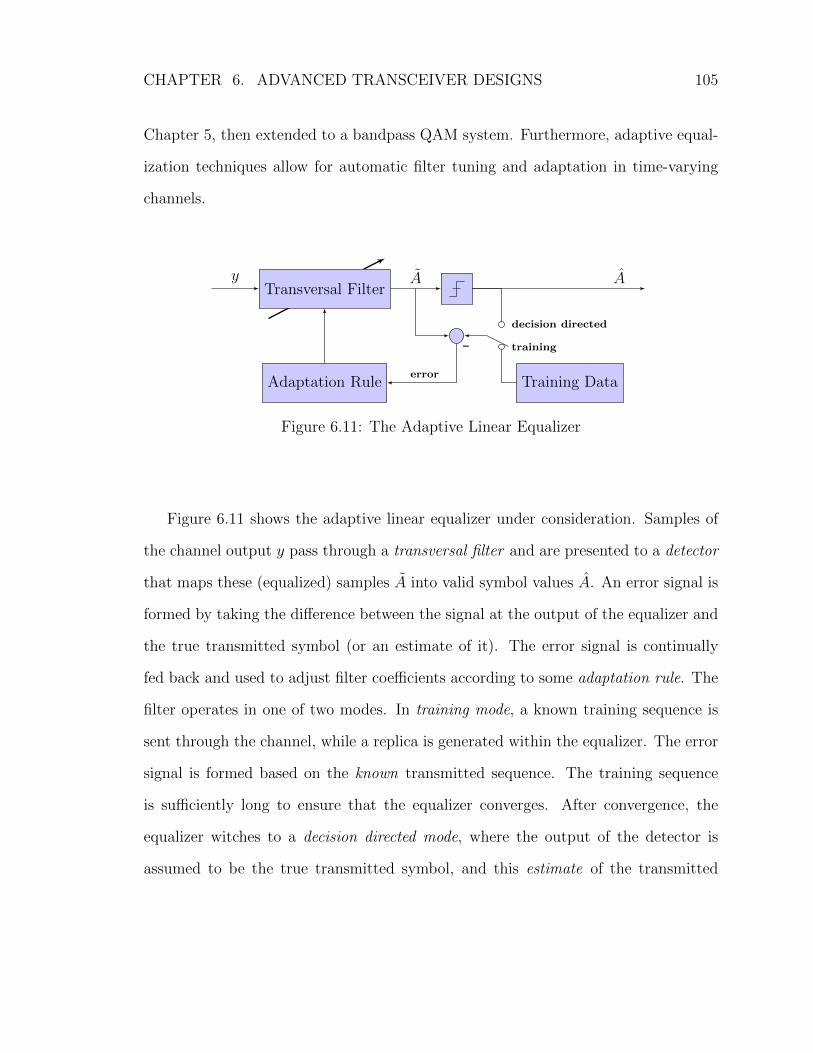
CHAPTER 6. ADVANCED TRANSCEIVER DESIGNS 105
Chapter 5, then extended to a bandpass QAM system. Furthermore, adaptive equal-
ization techniques allow for automatic filter tuning and adaptation in time-varying
channels.
Transversal Filtery A A
Adaptation Rule
decision directed
-error
Training Data
training
Figure 6.11: The Adaptive Linear Equalizer
Figure 6.11 shows the adaptive linear equalizer under consideration. Samples of
the channel output y pass through a transversal filter and are presented to a detector
that maps these (equalized) samples A into valid symbol values A. An error signal is
formed by taking the difference between the signal at the output of the equalizer and
the true transmitted symbol (or an estimate of it). The error signal is continually
fed back and used to adjust filter coefficients according to some adaptation rule. The
filter operates in one of two modes. In training mode, a known training sequence is
sent through the channel, while a replica is generated within the equalizer. The error
signal is formed based on the known transmitted sequence. The training sequence
is sufficiently long to ensure that the equalizer converges. After convergence, the
equalizer witches to a decision directed mode, where the output of the detector is
assumed to be the true transmitted symbol, and this estimate of the transmitted

CHAPTER 6. ADVANCED TRANSCEIVER DESIGNS 106
sequence is used for form the error signal. The transversal filter is described by
A[k] =
K2∑j=−K1
cj yk−j, (6.6)
where I[k] is the output of the filter at time k, c are the filter’s coefficients, and v
are filter input samples (channel output samples) spanning (k −K2 . . . k +K1). The
K1 anticausal filter taps counteract precursor ISI while the K2 causal taps counteract
postcursor ISI.
6.2.1 PAM Communication
We begin by applying the linear equalizer to the PAM equivalent channel intro-
duced in Chapter 5. Recall that the Gaussian pulse shape was used and symbols were
detected incoherently at the receiver. The width of the Gaussian pulse allowed us to
transmit at ts = 500 ns with zero pulse overlap. Figure 6.12 shows 1000 samples at
the output of the adaptive equalizer while in training mode, transmitting 2-PAM at
2 Msps. These are the same parameters used in the improved equalizer test of Sec-
tion 6.1.2. The filter employs the LMS algorithm to minimize the mean-squared value
of the error signal formed at the equalizer’s output. The result in Figure 6.12 shows
convergence after approximately 600 iterations. After convergence, the equalizer is
switched to decision directed mode for continual adaptation.
Achievable Data Rate The SNR measured at the output of the filter after training
is approximately 30 dB, allowing 8-PAM to be transmitted at a BER of less than 10−5.
The 99% pulse width of the Gaussian pulse is tpw = 1000 ns, yielding ts−min = 500 ns.
The achievable data rate using the linear equalizer is then
R = 3 bits/500 ns = 6.00 Mbps. (6.7)

CHAPTER 6. ADVANCED TRANSCEIVER DESIGNS 107
0 100 200 300 400 500 600 700 800 900 1000
0
0.2
0.4
0.6
0.8
1
Received symbol number
Equ
aliz
er o
utpu
t
Figure 6.12: Convergence of linear adaptive PAM equalizer
which is the same rate achieved with the improved equalizer. Both techniques result
a level of ISI suppression such that channel noise becomes the dominant factor that
limits data rate.
Filter Tap Allocation When considering the computational complexity of a linear
equalizer, the number of non-zero filter coefficients is of interest. The results in
Figure 6.12 were produced for the equalizer in Equation 6.7 having K1 = K2 = 12. It
is expected that due to the non-overlap of transmitted symbols, non-causal taps will
be zero valued (corresponding to zero precursor ISI). Furthermore, due to the sparse
nature of channel echoes, many of the causal taps will be zero valued as well [11].
Figure 6.13 shows the filter coefficients for the equalizer after training.
As expected, all non-causal taps are essentially zero-valued, and most causal taps
are as well. The tap corresponding to c0 is the filter’s direct feedthrough path. Al-
though the training algorithm has been performed on a 25 tap filter, substantial
computational reductions can be realized by allocating taps non-uniformly. Several
techniques are used in practice [11,12,61]. The simplest is to assign N available taps

CHAPTER 6. ADVANCED TRANSCEIVER DESIGNS 108
−10 −5 0 5 100
0.2
0.4
0.6
0.8
1
Tap number, cj
Tap
val
ue
Figure 6.13: Filter tap coefficients for PAM equalizer
to the N largest coefficients. Alternatively, a threshold can be applied to the tap
values and only those taps whose coefficients exceed that threshold survive. In this
example, applying a normalized threshold value of 0.01 to the taps results in only
three non-zero coefficients: c0, c-5, and c-9. The resulting equalizer experiences an
SNR degradation of less than 0.5 dB over the full 25 tap equalizer.
For the bulkhead test setup used throughout this study, the linear adaptive equal-
izer provides bit rate and BER comparable to that of the improved equalizer. Intel-
ligent allocation of filter taps has yielded an equalizer with very low computational
complexity. The complexity tradeoffs of the various equalizer methods will be dis-
cussed in greater detain in the following chapter.
6.2.2 QAM Communication
The communication techniques presented thus far have treated the communica-
tion channel as a baseband PAM channel. In reality, the resonant behavior of the
transmitting transducer acts as a Gaussian pulse shaper and upconverter, and com-

CHAPTER 6. ADVANCED TRANSCEIVER DESIGNS 109
munication occurs over a passband channel. Operating in this mode results in spec-
trally inefficient double sideband transmission. While the resulting system has low
complexity, it also yields relatively low throughput. By modulating separate PAM
symbol sequences on in-phase and quadrature carriers, the resulting QAM system can
achieve twice the throughput of the PAM system. Furthermore, Nyquest pulse shap-
ing can be accommodated, yielding better spectral efficiently and a further increase
in throughput.
Achievable Data Rate The ultrasonic channel in our lab test setup exhibits a
bandpass response with center frequency of 7.75 MHz and 3 dB bandwidth of approx-
imately 2.9 MHz. The channel’s 10 dB bandwidth is approximately 6.2 MHz. The I/Q
pulse shaping is accomplished using a root raised-cosine filter (RRCF) with symbol
frequency fs = 2.5 MHz and rolloff factor β = 0.5. At the receiver, another RRCF
functions as a matched filter, giving an overall raised-cosine (RC) response. After
modulation, the bandwidth occupied by the symbols stream is
BW = fs(1 + β) = 3.75 MHz (6.8)
The same adaptive filtering structure can be used with the QAM channel as was
used for PAM. The only difference is that the filter tap coefficients are complex
valued, and the filter processes complex valued channel samples. Figure 6.14 shows
the signal constellation at the output of the adaptive filter (the predetection point
A in Figure 6.11) after convergence when transmitting 64-QAM. The achievable bit
rate is 15 Mbps while maintaining a BER of 10−5.
Filter Tap Allocation Just as with the PAM transceiver, we apply a threshold to
the filter tap coefficients to remove those that are very near zero. The filter coefficients

CHAPTER 6. ADVANCED TRANSCEIVER DESIGNS 110
−1 0 1
−1
0
1
In−phase
Qua
drat
ure
Figure 6.14: Signal constellation after convergence of QAM linear equalizer
are shown in Figure 6.15. After thresholding the tap coefficients to eliminate those
whose normalized amplitude is less than 0.02, six non-zero taps remain.
−15 −10 −5 0 5 10 150
0.2
0.4
0.6
0.8
1
Tap number, cj
Tap
val
ue
Figure 6.15: Filter tap coefficients for QAM equalizer

CHAPTER 6. ADVANCED TRANSCEIVER DESIGNS 111
6.3 Orthogonal Frequency Division Multiplexing
Figure 6.16(a) shows the magnitude response of the ultrasonic channel introduced
in Chapter 4, without the bulkhead in place. The bandpass characteristic is due to the
frequency selective nature of the ultrasonic transducers. When the bulkhead is added
to the channel, it introduces the magnitude fluctuations shown in Figure 6.16(b).
Near the channel’s 7.75 MHz center frequency, the magnitude response fluctuates by
approximately 8 dB.
4 6 8 10 12 14 16−30
−20
−10
0
Frequency (MHz)
Mag
nitu
de (d
B)
(a) Without bulkhead
4 6 8 10 12 14 16−30
−20
−10
0
Frequency (MHz)
Mag
nitu
de (
dB)
(b) With bulkhead
Figure 6.16: Magnitude response of the ultrasonic channels
Orthogonal Frequency Division Multiplexing (OFDM) is well suited for commu-
nication over channels exhibiting spectral nulls in the passband, such as this one.
Because it divides the channel into numerous subcarriers (each occupying a small
fraction of the total bandwidth), an OFDM system can assign different modulation
schemes and power levels to each subcarrier to maximize total channel thoughput. A
subcarrier with high SNR may be assigned 64-QAM, while one with low SNR may
only be able to support 4-QAM. Furthermore, if a large number of subcarriers is

CHAPTER 6. ADVANCED TRANSCEIVER DESIGNS 112
chosen, the bandwidth of each can be made small enough that the channel is ap-
proximately flat over the subcarrier’s bandwidth. Under this condition, the channel
equalizer reduces to a single complex multiplication per subcarrier.
In our implementation, the passband is divided into 512 subcarrieres, spanning
a bandwidth of 8.33 MHz. The 60 subcarriers closest to ±Fs/2 are unused (set to
zero), giving 452 subcarriers, spanning a bandwidth of 7.35 MHz. A cyclic prefix of
70 symbols (8.4µs) is included to counteract channel echoes. The OFDM transceiver
operates in one of three modes: channel estimation mode, bit allocation mode, and
decision directed mode.
Channel Estimation In OFDM, the (flat) magnitude and phase errors experi-
enced by each subcarrier must be estimated and corrected for at the receiver, effec-
tively forming a single tap equalizer for each subcarrier. Through channel estimation,
the complex channel coefficient for each subcarrier is determined [62]. The techniques
used most commonly in practice make use of pilot tones transmitted either (1) pe-
riodically on all subcarriers (block type estimation), or (2) continually on several
dedicated subcarriers (comb type estimation) [63]. In the slowly time-varying ultra-
sonic channel, a simpler approach can be taken however.
Consider the symbol Aj transmitted over the j-th OFDM subcarrier. At the
output of the channel, the received symbol Aj is
Aj = cjAj (6.9)
where cj is the complex channel coefficient for that subcarrier, i.e. the scalar that
describes the magnitude and phase distortion the channel imparts to that subcarrier.
CHAPTER 6. ADVANCED TRANSCEIVER DESIGNS 113
If the coefficient is known, an equalizer can be formed for that subcarrier.
ej = 1/cj = Aj/Aj (6.10)
Over a noiseless channel, transmitting a single training symbol on each subcar-
rier (i.e. transmitting a single OFDM data block) is sufficient to extract the channel
coefficient vector. In a practical implementation, this coefficient estimation may be
performed over several training blocks so that noise can be filtered. In our imple-
mentation, the channel coefficient vector is estimated iteratively over several training
data blocks using
c[n] = (1− α)c[n− 1] + α(A/A) (6.11)
The channel coefficient vector c[n] at time n is a weighted sum of the past value
c[n − 1] and the current estimate A/A. This is an implementation of a discrete
time exponentially decaying filter where α controls the filter’s cutoff. Using our
experimental setup, a training period consisting of forty OFDM data blocks has been
used to produce a channel coefficient vector estimate.
Bit Allocation The maximum constellation size that each OFDM subcarrier can
support is determined by the SNR and required bit-error rate of the subcarrier. SNR
estimation of OFDM subcarriers can be performed several ways [64]. After the chan-
nel gain coefficients have been estimated and the equalizer applied to the channel, the
residual error at the output of the equalizer can be attributed to channel noise. In bit
allocation mode, a sequence of such noise samples is generated for each subcarrier,
and from these, an SNR estimate can be made for each subcarrier. Figure 6.17 shows
the normalized RMS noise measured on each subcarrier using the experimental setup.
For subcarriers near the center of the channel’s passband, where attenuation is low,
RMS noise is low. At the edges of the passband, where the channel’s attenuation is

CHAPTER 6. ADVANCED TRANSCEIVER DESIGNS 114
high, the high gain of the channel equalizer enhances noise.
0 50 100 150 200 250 300 350 400 450 5000
0.02
0.04
0.06
0.08
0.1
0.12
0.14
0.16
0.18
0.2
Subcarrier
RM
S n
oise
am
plitu
de (
norm
aliz
ed)
64−QAM
16−QAM
4−QAM
Figure 6.17: RMS noise measured on each OFDM subcarrier
The two dashed lines in the figure show the correspondence between subcarrier
RMS noise, and alphabet size. These thresholds are based on a required maximum
BER of 10−5. In Figure 6.18, signal constellations for three representative subcarriers
are shown. Subcarrier 50 (Figure 6.18(a)), with an SNR of approximately 15 dB can
only support 4-QAM. Subcarrier 255 on the other hand (Figure 6.18(a)) has an SNR
of 34 dB and can support 64-QAM.
Decision Directed After the channel coefficient vector is learned, the system
switches to a decision directed mode so that it can adapt to slowly time varying
channel conditions. In this mode, the output of the decision device is assumed to be
error free, and this data replaces the known transmitted sequence that was used in
training mode.
c[n] = (1− α)c[n− 1] + α(A/A) (6.12)

CHAPTER 6. ADVANCED TRANSCEIVER DESIGNS 115
−1 0 1
−1
0
1
In−phase
Qua
drat
ure
(a) Subcarrier 50, 4-QAM
−1 0 1
−1
0
1
In−phase
Qua
drat
ure
(b) Subcarrier 120, 16-QAM
−1 0 1
−1
0
1
In−phase
Qua
drat
ure
(c) Subcarrier 255, 64-QAM
Figure 6.18: OFDM subcarriers of differing constellation size
where A is the estimate of the transmitted symbol appearing at the output of the
detector.
Achievable Data Rate After bit allocation is completed, each OFDM subcarrier
is assigned a constellation size based on its SNR. The number of bits transmitted
during each OFDM frame is the sum of the bits conveyed on each subcarrier per
frame,
b =J∑j=1
bj. (6.13)
Implemented on our laboratory test setup, and based on the RMS noise estimates
shown in Figure 6.17, a block size of b = 2098 bits/frame was achieved. The OFDM
frame transmission rate is given by
f =BW
J + CP=
8.33 MHz
512 + 70= 14, 300 Hz (6.14)
where BW is the occupied bandwidth of the modulate signal, J is the number of
symbols transmitted per OFDM frame (i.e. the number of subcarriers) and CP is
the length of the cyclic prefix in symbols. The raw bit rate achieved by the OFDM

CHAPTER 6. ADVANCED TRANSCEIVER DESIGNS 116
system is
R = b · f = 2098 bits/frame · 14, 300 frames/sec ≈ 30.0 Mbps. (6.15)
6.4 Summary
In this chapter, several equalizer based ultrasonic transceivers have been devel-
oped. When implemented in the laboratory, these transceivers provide data rates in
the range of 2.68 Mbps to 30.0 Mbps. With this large spread in achievable data rates
comes an equally large spread in transceiver complexity. In the next chapter, the
hardware/software complexity of each transceiver introduced in this and the previ-
ous chapter will be discussed. With an understanding of the bandwidth-complexity
tradeoffs found in each technique, practitioners can choose the transceiver design that
best matches their application requirements.

117
7. Transceiver Hardware Implementation
In Chapters 5 and 6, several ultrasonic transceiver designs were presented, rang-
ing widely in achievable bitrate and complexity. In this chapter, we investigate the
implementation details associated with each transceiver so that the most appropriate
design can be selected for a given application.
To provide a common basis for comparing the complexity of each transceiver, the
same underlying hardware implementation (shown in Figure 7.1) will be assumed for
each. Data enters a digital signal processor (DSP) on the transmitting side of the
barrier. The data is processed and converted into a digital waveform that is then
sent to a digital-to-analog converter (D/A). The analog waveform generated by the
D/A passes through a reconstruction filter and a power amplifier before driving the
transmitting ultrasonic transducer.
DSP...101...
D/A PA tx rx A/D DSP...101...
Figure 7.1: Hardware implementation common to all transceivers
Signals sensed by the receiving transducer are first amplified then filtered by an
anti-aliasing filter before being digitized by an analog-to-digital converter (A/D). The
digital waveform is then sent to a second DSP which recovers the transmitted data
sequence and outputs it.
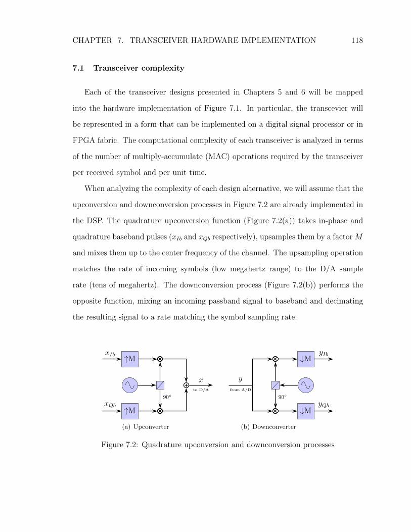
CHAPTER 7. TRANSCEIVER HARDWARE IMPLEMENTATION 118
7.1 Transceiver complexity
Each of the transceiver designs presented in Chapters 5 and 6 will be mapped
into the hardware implementation of Figure 7.1. In particular, the transcevier will
be represented in a form that can be implemented on a digital signal processor or in
FPGA fabric. The computational complexity of each transceiver is analyzed in terms
of the number of multiply-accumulate (MAC) operations required by the transceiver
per received symbol and per unit time.
When analyzing the complexity of each design alternative, we will assume that the
upconversion and downconversion processes in Figure 7.2 are already implemented in
the DSP. The quadrature upconversion function (Figure 7.2(a)) takes in-phase and
quadrature baseband pulses (xIb and xQb respectively), upsamples them by a factor M
and mixes them up to the center frequency of the channel. The upsampling operation
matches the rate of incoming symbols (low megahertz range) to the D/A sample
rate (tens of megahertz). The downconversion process (Figure 7.2(b)) performs the
opposite function, mixing an incoming passband signal to baseband and decimating
the resulting signal to a rate matching the symbol sampling rate.
↑MxIb
↑MxQb
90◦
xto D/A
(a) Upconverter
y
from A/D
90◦
↓M
↓M
yIb
yQb
(b) Downconverter
Figure 7.2: Quadrature upconversion and downconversion processes

CHAPTER 7. TRANSCEIVER HARDWARE IMPLEMENTATION 119
In the discussion the follows, we assume the following channel/transducer proper-
ties, in keeping with the laboratory test setup presented in Chapter 2.
Center frequency 7.75 MHz3 dB bandwidth 2.75 MHz10 dB bandwidth 6.20 MHz
7.1.1 Equalizer-free Transceivers
Figure 7.3 shows a block diagram of the equalizer-free transceiver discussed in
Chapters 5. Incoming symbols enter a pulse shaper which generates amplitude mod-
ulated excitation pulses that drive the transmitting transducer. At the receiver, an
envelope detector extracts the envelope of the received bandpass signal, and the de-
tector samples this envelope at the system’s symbol rate.
pulseshaper
tx rx envelopedetector
Aj Aj Aj
Figure 7.3: Block diagram of Equalizer-free Transceiver
Pulse Shaping The pulse shaper in a digital communication transmitter is gen-
erally implemented as an finite impulse response (FIR) filter. For this transceiver,
however, a simpler approach can be taken. Recall that with the equalizer-free tran-
sceiver, the transmitted symbol period is much longer than the width of the pulse
shaper’s output pulse, i.e., neighboring transmitted pulses do not overlap. This allows
us to implement the pulse shaper with a lookup table with N elements instead of an
N tap FIR filter. For each symbol to be transmitted, the pulse generater produces

CHAPTER 7. TRANSCEIVER HARDWARE IMPLEMENTATION 120
a sequence of N symbols. The length N is a function of the pulse duration and the
pulse shaper’s oversampling factor. Recall that the pulses generated with this tran-
sceiver are one-half cycle in length. If the pulse shaper uses a 4-to-1 oversampling
factor (as we have done in this implementation), the value of N is
N = 2 samples/cycle× 0.5 cycle× 4x oversampling = 4 samples (7.1)
The maximum symbol rate supported by the equalizer-free transceiver is approxi-
mately 1.34M samples/second. This results in 5.35M samples per second at the out-
put of the pulse generator. Modulating the amplitude of this pulse stream with the
incoming symbol stream requires one multiply-accumulate per pulse shaper sample
5.35 MMACs/sec (million MACs per second) or 4 MACs per symbol .
Envelope Detector Consider the real bandpass signal y(t) centered at fc Hz with
bandwidth BW Hz. Mixing the signal with an fc Hz quadrature carrier results in a
complex signal centered at DC, denoted yb(t). This signal can be expressed in either
rectangular or polar form.
yb(t) = yIb(t) + j yQb(t) = E2(t) ejφ(t)
where E2(t) = |yIb(t) + j yQb(t)|2 = yIb(t)2 + yQb(t)
2 is the squared envelope of the
complex signal, and φ(t) is its instantaneous phase.
{·}2
{·}2
yIb
yQb
Aj
Figure 7.4: Envelope detector block diagram
CHAPTER 7. TRANSCEIVER HARDWARE IMPLEMENTATION 121
Figure 7.4 shows the implementation of the envelope detector using the I and Q
outputs of the quadrature downconverter (Figure 7.2(b)). The I and Q components of
the signal yb[n], sampled at the transceiver’s symbol rate, are squared and summed,
producing E2[n] = x2[n] + x2[n]. Rather than calculate the square root of E2[n] and
present that value to the detector, a more computationally efficient technique is to
modify the detector’s decision thresholds to operate on E2[n] directly, eliminating
the square root operation entirely. The envelope detector requires 3 MAC operations
per symbol (two squaring operations and one summation). Operating at the rate of
1.34M samples/second, the block requires 4.02 MMACs/sec.
Overall Complexity The complexity of the complete equalizer-free transceiver
(pulse generator and envelope detector) is 7 MACs/symbol. When operating at
the maximum supported symbol rate of 1.34M symbols/second, this equates to 9.38
MMACs/sec. With each symbol encoding 1 bit, the maximum raw bitrate is 1.34
Mbps.
7.1.2 Channel Model Based Transceivers
An implementation of the channel model based transceiver (presented in Chap-
ter 6) is shown in Figure 7.5. This consists of a pulse shaper, envelope detector,
and equalizing filter. The pulse shaper and envelope detector are identical to those
implemented in the previous transceiver. The equalizer (not present in the previous
design), consists of an FIR filter and a delay element. In this transceiver, the equalizer
is derived directly from an estimated channel model. The complexity of the equalizer,
therefore, is dependant on which form of the channel model: the simplified model or
the improved model.

CHAPTER 7. TRANSCEIVER HARDWARE IMPLEMENTATION 122
pulseshaper
tx rx envelopedetector
AjAj Aj
El(z) z−d
−
Figure 7.5: Block diagram of Channel Model based Transceiver
Simplified Channel Model Based Transceiver
A channel equalizer based on the simplified channel model was presented in Sec-
tion 6.1.1. The assumption that the channel’s impulse response is an exponentially
decaying string of impulses lead the the following equalizer.
He(z) = 1− α z-r,
This equalizer requires exactly 1 MAC per input sample. The overall complexity of
the transceiver (including the pulse shaper and envelope detector), is 8 MACs/symbol.
At a symbol rate of 1.34M samples/second, this equates to 10.72 MMACs/sec. This
transceiver encodes 2 bits/symbol, yielding a maximum bitrate of 2.68 Mbps.
Improved Channel Model Based Transceiver
When the improved channel model is employed in the transceiver, the equalizer
takes the form
He(z) = 1− El(z)z-r,
El(z) =bE(1) + bE(2)z−1 + · · ·+ bE(ME + 1)z−ME
aE(1) + aE(2)z−1 + · · ·+ aE(NE + 1)z−NE

CHAPTER 7. TRANSCEIVER HARDWARE IMPLEMENTATION 123
i.e., El(z) in Figure 7.5 is an infinite impulse response (IIR) filter. The number of
multiply-accumulate operations needed per output from an IIR filter is equal to the
combined order of the numerator and denominator (ME + NE). We have shown in
Section 4.4.4 that for the ultrasonic lab setup, ME = 3, NE = 2. The complex-
ity of the IIR equalization filter, therefore, is 5 MACs/symbol. The overall com-
plexity of the transceiver (including the pulse shaper and envelope detector), is 12
MACs/symbol. The level of ISI suppression achieved with the improved transceiver
allows symbol rates of 2M symbols/second to be supported. At this rate, the com-
plexity of the improved transceiver is 24 MMACs/sec. This transceiver encodes 2
bits/symbol, yielding a maximum bitrate of 2.68 Mbps.
7.1.3 Linear Adaptive Equalizer Transceiver
Figure 7.6 shows the implementation of the linear equalizer based QAM transcei-
ver presented in Section 6.2. Incoming complex symbols are pulse shaped using a
root raised-cosine filter and upconverted to the channel’s center frequency using the
structure in Figure 7.2(a). At the receiver, the baseband signal is mixed down to
baseband, sent through a matched filter and linear equalizer, then passed to the de-
tector. We are interested in determining the complexity of the shaping and matched
filters, and the equalizer.
Shaping and matched filters The QAM transceiver in Section 6.2 achieved a
symbol rate of 2.5M symbols/sec using root raised-cosine pulse shaping. The shaping
filter was implemented using an FIR structure, and spanned five symbols. Oversam-
pling by a factor of two, this equates to a 20 tap filter. Implemented as a two path
polyphase filter [65], this filter has a workload of 20 multiply-accumulate operations
per input sample. The pulse shaper operates on complex symbols, requiring two iden-
tical real filters, one for the I path and one for the Q path. The overall workload of

CHAPTER 7. TRANSCEIVER HARDWARE IMPLEMENTATION 124
RRCF
ej2πf0
Re{·} tx
rx
ej2πf0
RRCF FIR FilterAj Aj
Aj
Figure 7.6: Block diagram of Linear Equalizer based Transceiver
the pulse shaper is then 40 MACs per input symbol. At 2.5M symbols/sec, this yields
100 MMACs/second. The matched filter at the receiver is implemented identically,
requiring an additional 40 MACs per symbol.
Equalizer The equalizing filter used in the QAM transceiver started as a twenty-
five tap FIR filter, After thresholding the taps to remove the negligibly small tap
coefficients, only six taps remained. This results in a workload of 6 MACs per symbol,
or 15M MMACs/second, for each of the I and Q paths.
Overall Complexity Between the pulse shaping filter, matched filter, and and
equalizer, the linear QAM transceiver has a complexity of 92 MACs per symbol. At
a symbol rate of 2.5M symbols/sec, this equates to 230M MACs/second. Encoding 6
bits/symbol (three on the in-phase carrier and three on the quadrature carrier), the
achievable data rate of the QAM transceiver is 15 Mbps.
7.1.4 OFDM Transceiver
An implementation of the OFDM transceiver is shown in Figure 7.7. Incoming
QAM symbols are sent onto an N-point inverse FFT, generating an N-point time

CHAPTER 7. TRANSCEIVER HARDWARE IMPLEMENTATION 125
series. A cyclic prefix is concatenated with the sequence. The signal is mixed up to a
carrier frequency and transmitted. At the receiver, the signal is mixed down to DC.
The resulting complex baseband signal has its cyclic prefix stripped and is processed
by an FFT that recovers (unequalized) transmitted symbol samples. The samples are
equalized and sent to a detector, where the transmitted symbols are recovered.
Aj IFFT... P/S...
AddCyclicPrefix
ej2πf0
Re{·} tx
rx
ej2πf0
RemoveCyclicPrefix
S/P FFT... EQ...... Aj
...
Figure 7.7: Block diagram of OFDM Transceiver
The complexity of the OFDM transceiver is primarily a function of the FFT blocks
and the equalizer. The parallel/serial conversion and cyclic prefix addition/removal
blocks contribute noting to the transceiver’s complexity.
IFFT and FFT Stages The OFDM transceiver designed in Chapter 6 uses a
512-point FFT, generating 452 subcarriers. The remaining sixty subcarrier (thirty
located near Fs/2 and thirty located at −Fs/2) are zero-valued to eliminate spec-
tral content near the folding frequency. The complexity of the IFFT operation per
OFDM frame is N logN multiply-accumulate operations, where N = 512. With each

CHAPTER 7. TRANSCEIVER HARDWARE IMPLEMENTATION 126
OFDM frame transmitting 452 symbols, the complexity if the IFFT block is 4608
complex MACs/frame (9216 real MACs/frame) or 10.2 complex MACs/symbol (20.4
real MACs/symbol). The complexity of the FFT operation at the receiver is identical.
Equalizer In an OFDM transceiver, the width of each subcarrier can be made
sufficiently small that the channel’s magnitude and phased distortions over the sub-
carrier’s bandwidth is approximately constant. The equalizer for that subcarrier,
therefore is a scalar multiplier. The equalizer for each subcarrier then requires 452
complex MACs/frame (904 real MACs/frame) or 1 complex MACs/symbol (2 real
MACs/symbol).
Overall Complexity Between IFFT, FFT, and equalizer stages, the OFDM tran-
sceiver has a complexity of 19,300 MACs/frame or 42.8 MACs/symbol. At the tran-
sceiver’s maximum frame rate of 14,300 frames/sec, this equates to 276 MMACs/sec.
The maximum throughput of the OFDM transceiver is 30 Mbps.
7.2 Comparison of Techniques
Table 7.1 shows a comparison of the computational requirements for each transcei-
ver under consideration. The maximum symbol rate and the number of bits encoded
per symbol are given, along with the maximum achievable bitrate. Each transceiver’s
complexity is reported per symbol, per bit, and per second. The latter value assumes
that the transceiver is operating at its maximum data rate. Knowing complexity
per bit allows us to compare transceivers relative to one another, while knowing
complexity per second indicates the computational power needed to implement the
transceiver.
The data in Table 7.1 shows that the equalizer-free transceiver requires the fewest
computations per received symbol. Since the model-based transceivers can encode
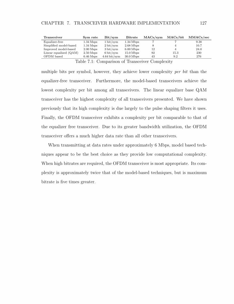
CHAPTER 7. TRANSCEIVER HARDWARE IMPLEMENTATION 127
Transceiver Sym rate Bit/sym Bitrate MACs/sym MACs/bit MMACs/sec
Equalizer-free 1.34 Msps 1 bit/sym 1.34 Mbps 7 7 9.38Simplified model-based 1.34 Msps 2 bit/sym 2.68 Mbps 8 4 10.7Improved model-based 2.00 Msps 3 bit/sym 6.00 Mbps 12 4 24.0Linear equalized (QAM) 2.50 Msps 6 bit/sym 15.0 Mbps 92 15.3 230OFDM based 6.46 Msps 4.64 bit/sym 30.0 Mbps 43 9.2 276
Table 7.1: Comparison of Transceiver Complexity
multiple bits per symbol, however, they achieve lower complexity per bit than the
equalizer-free transceiver. Furthermore, the model-based transceivers achieve the
lowest complexity per bit among all transceivers. The linear equalizer base QAM
transceiver has the highest complexity of all transceivers presented. We have shown
previously that its high complexity is due largely to the pulse shaping filters it uses.
Finally, the OFDM transceiver exhibits a complexity per bit comparable to that of
the equalizer free transceiver. Due to its greater bandwidth utilization, the OFDM
transceiver offers a much higher data rate than all other transceivers.
When transmitting at data rates under approximately 6 Mbps, model based tech-
niques appear to be the best choice as they provide low computational complexity.
When high bitrates are required, the OFDM transceiver is most appropriate. Its com-
plexity is approximately twice that of the model-based techniques, but is maximum
bitrate is five times greater.

128
Concluding Remarks
In this thesis, we have presented techniques for achieving high bitrate communica-
tion across metallic barriers using ultrasonic signaling. A simulation model has been
developed, and a procedure for tuning the model using experimental data has been
presented. We have shown that this model accurately captures the echoing charac-
teristics that make high bitrate communication in the ultrasonic channel a challenge.
Several transceiver designs have been developed and compared in terms of their
computational complexity. The transceivers chosen in this study were intended to
cover a wide range of data rate requirements. After comparing the computational
requirements of the transceivers, we have concluded that two of these designs are
particularly attractive. For low bitrate applications, model based transceivers provide
a low complexity alternative. The OFDM transceiver, on the other hand, provides
high data rate at the expense of greater computational complexity.
In recent years, ultrasonic through-metal communication techniques have been
adapted to a variety of applications ranging greatly in bit rate requirements and
power consumption constraints. This thesis provides tools to allow designers to im-
plement the through-metal transceiver that is best matched to the requirements and
constraints of their application.


Bibliography
[1] A. Seman, M. Donnelly, and S. Mastro, “Wireless systems development for dis-tributed machinery monitoring and control,” American Society of Naval Engi-neers (ASNE) Intelligent Ships Symposium VII, May 2007.
[2] C. Zacot, “Shipboard wireless sensor networks utilizing zigbee technology,” Mas-ter’s thesis, Naval Postgraduate School, Monterey, CA, 2006.
[3] T. Murphy, “Ultrasonic Digital Communication System for a Steel Wall Multi-path Channel: Methods and Results,” Master’s thesis, Rensselaer PolytechnicInstitute, 2006.
[4] G. J. Saulnier, H. A. Scarton, A. J. Gavens, D. A. Shoudy, T. L. Murphy, M. Wet-zel, S. Bard, S. Roa-Prada, and P. Das, “P1g-4 through-wall communication oflow-rate digital data using ultrasound,” in Ultrasonics Symposium, 2006. IEEE,Oct. 2006, pp. 1385–1389.
[5] D. Shoudy, G. Saulnier, H. Scarton, P. Das, S. Roa-Prada, J. Ashdown, andA. Gavens, “P3f-5 an ultrasonic through-wall communication system with powerharvesting,” in Ultrasonics Symposium, 2007. IEEE, Oct. 2007, pp. 1848–1853.
[6] M. Kluge, T. Becker, J. Schalk, and T. Otterpohl, “Remote acoustic poweringand data transmission for sensors inside of conductive envelopes,” in Sensors,2008 IEEE, Oct. 2008, pp. 41–44.
[7] D. Graham, J. Neasham, and B. Sharif, “High bit rate communication throughmetallic structures using electromagnetic acoustic transducers,” in OCEANS2009-EUROPE, 2009. OCEANS ’09., May 2009, pp. 1–6.
[8] P. Smalser, “Power transfer of piezoelectric generated energy,” Dec. 30 1997, USPatent 5,703,474.
[9] Y. Hu, X. Zhang, J. Yang, and Q. Jiang, “Transmitting electric energy througha metal wall by acoustic waves using piezoelectric transducers,” Ultrasonics,Ferroelectrics and Frequency Control, IEEE Transactions on, vol. 50, no. 7, pp.773–781, July 2003.
[10] S. Sherrit, B. Doty, M. Badescu, X. Bao, Y. Bar-Cohen, J. Aldrich, and Z. Chang,“Studies of acoustic-electric feed-throughs for power transmission through struc-tures.” 2006.
[11] F. Lee and P. McLane, “Design of nonuniformly spaced tapped-delay-line equal-izers for sparse multipath channels,” Communications, IEEE Transactions on,vol. 52, no. 4, pp. 530–535, April 2004.

[12] I. Fevrier, S. Gelfand, and M. Fitz, “Reduced complexity decision feedback equal-ization for multipath channels with large delay spreads,” Communications, IEEETransactions on, vol. 47, no. 6, pp. 927–937, Jun 1999.
[13] S. Haykin, Adaptive Filter Theory, 4th ed. Prentice hall, 2001.
[14] T. Street, X. Nguyen, and F. Williams, “Wireless Communication Technologieson ex-USS Shadwell,” Naval Research Laboratory, Washington DC, 2002.
[15] T. Brooks, K. B. Lee, and S. Chen, “IEEE 1451 Smart Wireless Machinery Mon-itoring and Control for Naval Vessels,” in Thirteenth International Ship ControlSystems Symposium (SCSS), April 2003.
[16] “Panametrics-NDT ultrasonic transducers for nondestructive testing,” OlympusNDT, p. 8, 2009.
[17] “Ultrasonic transducers technical notes,” Olympus NDT, 2009.
[18] J. Proakis and M. Salehi, Digital Communications, 5th ed. McGraw-Hill NewYork, 2008.
[19] H. Seki, A. Granato, and R. Truell, “Diffraction effects in the ultrasonic field of apiston source and their importance in the accurate measurement of attenuation,”The Journal of the Acoustical Society of America, vol. 28, no. 2, pp. 230–238,1956.
[20] G. S. Smith, An Introduction to Classical Electromagnetic Radiation. CambridgeUniversity Press, 1997.
[21] C. Dang, L. Schmerr Jr, and A. Sedov, “Modeling and measuring all the elementsof an ultrasonic nondestructive evaluation system I: modeling foundations,” Re-search in Nondestructive Evaluation, vol. 14, no. 3, pp. 141–176, 2002.
[22] L. Schmerr, A. Lopez-Sanchez, and R. Huang, “Complete ultrasonic transducercharacterization and its use for models and measurements,” Ultrasonics, vol. 44,pp. 753–757, 2006.
[23] W. Leach, “Controlled-source analogous circuits and SPICE models for piezo-electric transducers,” IEEE Transactions on Ultrasonics, Ferroelectrics, and Fre-quency Control, vol. 41, no. 1, pp. 60–66, 1994.
[24] I. Hallaj and R. Cleveland, “FDTD simulation of finite-amplitude pressure andtemperature fields for biomedical ultrasound,” JOURNAL-ACOUSTICAL SO-CIETY OF AMERICA, vol. 105, pp. 7–12, 1999.
[25] D. Kilfoyle and A. Baggeroer, “The state of the art in underwater acoustictelemetry,” IEEE Journal of Oceanic Engineering, vol. 25, no. 1, pp. 4–27, 2000.

[26] M. Chitre, S. Shahabudeen, and M. Stojanovic, “Underwater acoustic commu-nications and networking: Recent advances and future challenges,” The State ofTechnology in 2008, vol. 42, no. 1, pp. 103–114, 2008.
[27] N. Priyantha, A. Chakraborty, and H. Balakrishnan, “The cricket location-support system,” in Proceedings of the 6th annual international conference onMobile computing and networking. ACM New York, NY, USA, 2000, pp. 32–43.
[28] C. Lopes and P. Aguiar, “Acoustic modems for ubiquitous computing,” PervasiveComputing, IEEE, vol. 2, no. 3, pp. 62–71, July-Sept. 2003.
[29] R. Welle, “Ultrasonic data communication system,” Nov. 9 1999, US Patent5,982,297.
[30] ——, “Ultrasonic power sensory system,” Oct. 3 2000, US Patent 6,127,942.
[31] R. Payton, “System for acoustically passing electrical signals through a hull,”Sept. 23 2003, US Patent 6,625,084.
[32] Z. tao Yang, S. hua Guo, Y. tai Hu, and J. shi Yang, “Modeling of power trans-mission through an elastic wall by piezoelectric transducers and acoustic waves,”in Piezoelectricity, Acoustic Waves, and Device Applications, 2008. SPAWDA2008. Symposium on, Dec. 2008, pp. 93–97.
[33] W. Na and T. Kundu, “A combination of PZT and EMAT transducers for in-terface inspection,” The Journal of the Acoustical Society of America, vol. 111,p. 2128, 2002.
[34] W. Mason, “Electromechanical transducers and wave filters,” 1948.
[35] R. Krimholtz, D. Leedom, and G. Matthaei, “New equivalent circuits for ele-mentary piezoelectric transducers,” Electronics Letters, vol. 6, p. 398, 1970.
[36] M. Redwood, “Transient performance of a piezoelectric transducer,” The Journalof the Acoustical Society of America, vol. 33, p. 527, 1961.
[37] S. Morris and C. Hutchens, “Implementation of mason’s model on circuit anal-ysis programs,” Ultrasonics, Ferroelectrics and Frequency Control, IEEE Trans-actions on, vol. 33, no. 3, pp. 295–298, May 1986.
[38] A. Puttmer, P. Hauptmann, R. Lucklum, O. Krause, and B. Henning, “Spicemodel for lossy piezoceramic transducers,” Ultrasonics, Ferroelectrics and Fre-quency Control, IEEE Transactions on, vol. 44, no. 1, pp. 60–66, Jan 1997.
[39] R. Cobbold, Foundations of biomedical ultrasound. Oxford University Press,USA, 2006.
[40] A. Arnau, Piezoelectric transducers and applications. Springer Verlag, 2008.

[41] J. van Deventer, T. Lofqvist, and J. Delsing, “Pspice simulation of ultrasonicsystems,” Ultrasonics, Ferroelectrics and Frequency Control, IEEE Transactionson, vol. 47, no. 4, pp. 1014–1024, Jul 2000.
[42] C. Dang, L. Schmerr Jr, and A. Sedov, “Modeling and Measuring All the Ele-ments of an Ultrasonic Nondestructive Evaluation System II: Model-Based Mea-surements,” Research in Nondestructive Evaluation, vol. 14, no. 4, pp. 177–201,2002.
[43] L. Capineri, L. Masotti, M. Rinieri, and S. Rocchi, “Ultrasonic transducers as ablack-box: equivalent circuit synthesis and matching network design,” Ultrason-ics, Ferroelectrics and Frequency Control, IEEE Transactions on, vol. 40, no. 6,pp. 694–703, Nov 1993.
[44] G. Jacovitti and G. Scarano, “Discrete time techniques for time delay estima-tion,” Signal Processing, IEEE Transactions on, vol. 41, no. 2, pp. 525–533, Feb1993.
[45] A. Grennberg and M. Sandell, “Estimation of subsample time delay differencesin narrowband ultrasonic echoes using the hilbert transform correlation,” Ul-trasonics, Ferroelectrics and Frequency Control, IEEE Transactions on, vol. 41,no. 5, pp. 588–595, Sep 1994.
[46] R. Demirli and J. Saniie, “Model-based estimation of ultrasonic echoes. PartI: Analysis and algorithms,” Ultrasonics, Ferroelectrics and Frequency Control,IEEE Transactions on, vol. 48, no. 3, pp. 787–802, May 2001.
[47] Y. Lu, R. Demirli, and J. Saniie, “3E-3 A Comparative Study of Echo EstimationTechniques for Ultrasonic NDE Applications,” in IEEE Ultrasonics Symposium,2006, 2006, pp. 436–439.
[48] B. Widrow, Adaptive Filters I: Fundamentals. Electronics Laboratories StanfordUniversity, 1966.
[49] B. Sklar, Digital Communications: Fundamentals and Applications, 2nd ed.Prentice-Hall Englewood Cliffs, NJ, 2001.
[50] M. Austin, “Decision-feedback equalization for digital communication over dis-persive channels.” 1967.
[51] D. George, R. Bowen, and J. Storey, “An adaptive decision feedback equalizer,”Communication Technology, IEEE Transactions on, vol. 19, no. 3, pp. 281–293,June 1971.
[52] S. Altekar and N. Beaulieu, “Upper bounds to the error probability of deci-sion feedback equalization,” Information Theory, IEEE Transactions on, vol. 39,no. 1, pp. 145–156, Jan 1993.

[53] R. Kumar, “Convergence of a decision-directed adaptive equalizer,” in Decisionand Control, 1983. The 22nd IEEE Conference on, vol. 22, dec. 1983, pp. 1319–1324.
[54] R. Johnson, P. Schniter, T. Endres, J. Behm, D. Brown, and R. Casas, “Blindequalization using the constant modulus criterion: A review,” Proceedings of theIEEE, vol. 86, no. 10, pp. 1927–1950, 1998.
[55] A. Sayed, Fundamentals of Adaptive Filtering. Wiley-IEEE Press, 2003.
[56] K. Yee, “Numerical solution of initial boundary value problems involvingmaxwell’s equations in isotropic media,” Antennas and Propagation, IEEETransactions on, vol. 14, no. 3, pp. 302 –307, may 1966.
[57] M. Cizek and J. Rozman, “Acoustic wave equation simulation using FDTD,”april 2007, pp. 1 –4.
[58] K. Steiglitz and L. McBride, “A technique for the identification of linear sys-tems,” Automatic Control, IEEE Transactions on, vol. 10, no. 4, pp. 461–464,Oct 1965.
[59] R. Fourer, D. M. Gay, and B. Kernighan, AMPL: A Modeling Language forMathematical Programming. Duxbury Press, 2002.
[60] Optimization Toolbox 5 Users Guide, The MathWorks, Inc., 2010.
[61] A. Rontogiannis and K. Berberidis, “Efficient decision feedback equalizationfor sparse wireless channels,” Wireless Communications, IEEE Transactions on,vol. 2, no. 3, pp. 570–581, May 2003.
[62] V. Srivastava, C. Ho, P. Fung, and S. Sun, “Robust MMSE channel estimation inOFDM systems with practical timing synchronization,” in 2004 IEEE WirelessCommunications and Networking Conference, 2004. WCNC, vol. 2, 2004.
[63] S. Coleri, M. Ergen, A. Puri, and A. Bahai, “Channel estimation techniquesbased on pilot arrangement in OFDM systems,” IEEE Transactions on Broad-casting, vol. 48, no. 3, pp. 223–229, 2002.
[64] H. Arslan and S. Reddy, “Noise power and SNR estimation for OFDM basedwireless communication systems,” in Proc. of 3rd IASTED International Confer-ence on Wireless and Optical Communications (WOC), Banff, Alberta, Canada,2003.
[65] F. J. Harris, Multirate Signal Processing for Communication Systems. PrenticeHall, 2004.