hierarchical self organizing map based ids on kdd …
TRANSCRIPT

HIERARCHICAL SELF ORGANIZING MAP BASED IDS
ON KDD BENCHMARK
By
Hilmi Gunes Kayacık
SUBMITTED IN PARTIAL FULFILLMENT OF THE
REQUIREMENTS FOR THE DEGREE OF
MASTER OF SCIENCE
AT
DALHOUSIE UNIVERSITY
HALIFAX, NOVA SCOTIA
c© Copyright by Hilmi Gunes Kayacık, 2003

DALHOUSIE UNIVERSITY
FACULTY OF
COMPUTER SCIENCE
The undersigned hereby certify that they have read and recommend
to the Faculty of Graduate Studies for acceptance a thesis entitled
“HIERARCHICAL SELF ORGANIZING MAP BASED IDS ON
KDD BENCHMARK ” by Hilmi G unes Kayacıkin partial fulfillment of the
requirements for the degree ofMaster of Science.
Dated:
Supervisors:Dr. Nur Zincir-Heywood
Dr. Malcolm I. Heywood
Readers:Dr. Raza Abidi
Dr. Murray Heggie
ii

DALHOUSIE UNIVERSITY
Date:
Author: Hilmi G unes Kayacık
Title: HIERARCHICAL SELF ORGANIZING MAP BASED
IDS ON KDD BENCHMARK
Faculty: Computer Science
Degree:M.Sc. Convocation:May Year: 2003
Permission is herewith granted to Dalhousie University to circulate and tohave copied for non-commercial purposes, at its discretion, the above title upon therequest of individuals or institutions.
Signature of Author
THE AUTHOR RESERVES OTHER PUBLICATION RIGHTS, AND NEITHERTHE THESIS NOR EXTENSIVE EXTRACTS FROM IT MAY BE PRINTED OROTHERWISE REPRODUCED WITHOUT THE AUTHOR’S WRITTEN PERMISSION.
THE AUTHOR ATTESTS THAT PERMISSION HAS BEEN OBTAINEDFOR THE USE OF ANY COPYRIGHTED MATERIAL APPEARING IN THISTHESIS (OTHER THAN BRIEF EXCERPTS REQUIRING ONLY PROPERACKNOWLEDGEMENT IN SCHOLARLY WRITING) AND THAT ALL SUCHUSE IS CLEARLY ACKNOWLEDGED.
iii

Contents
List of Tables vii
List of Figures x
Abstract xiii
Acknowledgements xiv
1 Introduction 1
2 Literature Survey 6
2.1 Learning System Approaches . . . . . . . . . . . . . . . . . . . . . . . . . 6
2.2 Signature Based Intrusion Detection . . . . . . . . . . . . . . . . . . . . . 20
2.2.1 Examples Signature Based Systems . . . . . . . . . . . . . . . . . 21
2.2.2 Benchmarking Test Set-up and Procedures . . . . . . . . . . . . . 23
2.2.3 Evaluation Results . . . . . . . . . . . . . . . . . . . . . . . . . . 26
iv

2.3 Discussion . . . . . . . . . . . . . . . . . . . . . . . . . . . . . . . . . . . 30
3 Methodology 32
3.1 The Dataset . . . . . . . . . . . . . . . . . . . . . . . . . . . . . . . . . . 32
3.1.1 Collected Data: DARPA 98 Dataset . . . . . . . . . . . . . . . . . 33
3.1.2 Summarized Data: KDD 99 Dataset . . . . . . . . . . . . . . . . . 34
3.2 Multi Level Hierarchy . . . . . . . . . . . . . . . . . . . . . . . . . . . . 36
3.3 Pre-Processing and Clustering . . . . . . . . . . . . . . . . . . . . . . . . 38
3.3.1 1st Level Pre-Processing . . . . . . . . . . . . . . . . . . . . . . . 38
3.3.2 2nd Level Pre-Processing . . . . . . . . . . . . . . . . . . . . . . . 40
3.3.3 3rd Level Pre-Processing . . . . . . . . . . . . . . . . . . . . . . . 40
4 Learning Algorithms 42
4.1 Self-Organizing Maps . . . . . . . . . . . . . . . . . . . . . . . . . . . . . 42
4.2 Potential Function Clustering . . . . . . . . . . . . . . . . . . . . . . . . . 48
5 Results 51
5.1 KDD 99 Dataset . . . . . . . . . . . . . . . . . . . . . . . . . . . . . . . . 51
5.2 Training Parameters . . . . . . . . . . . . . . . . . . . . . . . . . . . . . . 52
5.3 Experiments . . . . . . . . . . . . . . . . . . . . . . . . . . . . . . . . . . 53
5.3.1 Experiments on Training Set Biases . . . . . . . . . . . . . . . . . 54
v

5.3.2 Experiments on Third Layer Maps . . . . . . . . . . . . . . . . . . 60
5.3.3 Experiments on Feature Contribution . . . . . . . . . . . . . . . . 73
5.4 Comparisons . . . . . . . . . . . . . . . . . . . . . . . . . . . . . . . . . 77
6 Conclusions and Future Work 78
Appendix A KDD 99 Dataset Details 83
Appendix B Detailed Detection Rates 89
Appendix C U-Matrix Displays of the 2nd Level SOMs in Section 5.3.1 93
Appendix D U-Matrix and Labels of the 2nd Level SOMs in Section 5.3.3 95
Bibliography 99
vi

List of Tables
2.1 Complexity data of the three detection models . . . . . . . . . . . . . . . . 10
2.2 Acuracy of the KDD 99 winner on different categories . . . . . . . . . . . 11
2.3 Performance summary of the KDD 99 winners. . . . . . . . . . . . . . . . 13
2.4 Performance of the three learning algorithms on KDD 99 data . . . . . . . 15
2.5 Summary of the confidence rules . . . . . . . . . . . . . . . . . . . . . . . 26
2.6 Number of detected attack instances in different categories compared with
their number of occurrences in 4th week . . . . . . . . . . . . . . . . . . . 26
2.7 Detection confidence rules for each system . . . . . . . . . . . . . . . . . . 27
2.8 Distribution of triggered Cisco IOS signatures among attack related entries . 28
5.1 Basic Characteristics of the KDD dataset . . . . . . . . . . . . . . . . . . . 52
5.2 SOM Training Parameters . . . . . . . . . . . . . . . . . . . . . . . . . . 53
5.3 Shift Register Parameters . . . . . . . . . . . . . . . . . . . . . . . . . . . 53
5.4 Basic Characteristics of the three training datasets Employed . . . . . . . . 54
5.5 Potential Function Parameters . . . . . . . . . . . . . . . . . . . . . . . . 54
vii

5.6 Test Set Results for the first training data set . . . . . . . . . . . . . . . . . 56
5.7 Test Set Results for the Second training data set . . . . . . . . . . . . . . . 57
5.8 Test Set Results for the third training data set . . . . . . . . . . . . . . . . 59
5.9 Performance of the three systems on different categories . . . . . . . . . . 59
5.10 Detection rate of new attacks for three systems . . . . . . . . . . . . . . . 60
5.11 Count of Attack and Normal connections per 2nd layer candidate neuron . . 61
5.12 Test Set Results of second and third level hierarchies . . . . . . . . . . . . 72
5.13 Performance of two layer and three layer hierarchies on different categories 73
5.14 Detection rate of new attacks for two-layer and three-layer hierarchy . . . . 73
5.15 Contribution results on Corrected test set . . . . . . . . . . . . . . . . . . . 75
5.16 Performance of the systems excluding one feature on different categories . . 75
5.17 Performance of the systems excluding one feature on new attacks . . . . . . 76
5.18 Recent Results on the KDD benchmark . . . . . . . . . . . . . . . . . . . 77
5.19 Performance of the KDD 99 winner . . . . . . . . . . . . . . . . . . . . . 77
A.1 Label counts of the KDD 99 datasets . . . . . . . . . . . . . . . . . . . . . 83
A.2 Enumeration of the alphanumeric Protocol feature . . . . . . . . . . . . . . 85
A.3 Enumeration of the alphanumeric Service feature . . . . . . . . . . . . . . 85
A.4 Enumeration of the Bro Flag feature . . . . . . . . . . . . . . . . . . . . . 88
viii

B.1 Detection rates for each attack type for systems explained in section 5.3.1
and 5.3.2 . . . . . . . . . . . . . . . . . . . . . . . . . . . . . . . . . . . . 89
B.2 Detection rates for each attack type for feature contribution experiments in
Section 5.3.3 . . . . . . . . . . . . . . . . . . . . . . . . . . . . . . . . . 90
ix

List of Figures
2.1 Decision tree for smurf attack [19] . . . . . . . . . . . . . . . . . . . . . . 12
2.2 Network diagram of the benchmarking environment . . . . . . . . . . . . . 24
2.3 Log file analysis in terms of number of entries . . . . . . . . . . . . . . . . 27
2.4 Analysis of detected attacks . . . . . . . . . . . . . . . . . . . . . . . . . . 29
2.5 Performance of the evaluated systems . . . . . . . . . . . . . . . . . . . . 30
3.1 Simplified version of DARPA 98 Simulation Network . . . . . . . . . . . . 33
3.2 Multi Layer SOM-Architecture . . . . . . . . . . . . . . . . . . . . . . . . 37
3.3 Shift register with taps shown in white cells and intervals shown in gray cells 39
4.1 SOM in output space . . . . . . . . . . . . . . . . . . . . . . . . . . . . . 45
4.2 SOM before and after training in input space . . . . . . . . . . . . . . . . . 45
4.3 U-Matrix of the Example SOM . . . . . . . . . . . . . . . . . . . . . . . . 46
4.4 Hit histogram for the example SOM . . . . . . . . . . . . . . . . . . . . . 47
4.5 Labels of the example SOM . . . . . . . . . . . . . . . . . . . . . . . . . 48
x

5.1 Hit histogram of the second level map for the 10% KDD dataset . . . . . . 55
5.2 Neurons Labels of the Second Level Map trained on 10%KDD dataset . . . 56
5.3 Hit histogram of the second level map for the normal only 10% KDD dataset 56
5.4 Neurons Labels of the Second Level Map trained on normal only 10%KDD
dataset . . . . . . . . . . . . . . . . . . . . . . . . . . . . . . . . . . . . . 57
5.5 Hit histogram of the second level map for the 50/50 dataset . . . . . . . . . 58
5.6 Neurons Labels of the Second Level Map for the 50/50 dataset . . . . . . . 59
5.7 U-Matrix of the neuron 36 third level map . . . . . . . . . . . . . . . . . . 61
5.8 Hit histogram of the neuron 36 third level map . . . . . . . . . . . . . . . . 62
5.9 Neuron Labels of the neuron 36 third level map . . . . . . . . . . . . . . . 62
5.10 U-Matrix of the neuron 4 third level map . . . . . . . . . . . . . . . . . . . 63
5.11 Hit histogram of the neuron 4 third level map . . . . . . . . . . . . . . . . 63
5.12 Neuron Labels of the neuron 4 third level map . . . . . . . . . . . . . . . . 64
5.13 U-Matrix of the neuron 17 third level map . . . . . . . . . . . . . . . . . . 65
5.14 Hit histogram of the neuron 17 third level map . . . . . . . . . . . . . . . . 65
5.15 Neuron Labels of the neuron 17 third level map . . . . . . . . . . . . . . . 66
5.16 U-Matrix of the neuron 18 third level map . . . . . . . . . . . . . . . . . . 67
5.17 Hit histogram of the neuron 18 third level map . . . . . . . . . . . . . . . . 67
5.18 Neuron Labels of the neuron 18 third level map . . . . . . . . . . . . . . . 68
5.19 U-Matrix of the neuron 23 third level map . . . . . . . . . . . . . . . . . . 69
xi

5.20 Hit histogram of the neuron 23 third level map . . . . . . . . . . . . . . . . 69
5.21 Neuron Labels of the neuron 23 third level map . . . . . . . . . . . . . . . 70
5.22 U-Matrix of the neuron 30 third level map . . . . . . . . . . . . . . . . . . 71
5.23 Hit histogram of the neuron 30 third level map . . . . . . . . . . . . . . . . 71
5.24 Neuron Labels of the neuron 30 third level map . . . . . . . . . . . . . . . 72
C.1 U-Matrix of the second level map for the 10% KDD dataset . . . . . . . . . 93
C.2 U-Matrix of the second level map for the normal only10% KDD dataset . . 94
C.3 U-Matrix of the second level map for the 50/50 dataset . . . . . . . . . . . 94
D.1 U-matrix and labels for the baseline 36 dimensional second level map (Sys-
tem 1) . . . . . . . . . . . . . . . . . . . . . . . . . . . . . . . . . . . . . 95
D.2 U-matrix and labels for the duration excluded second level map . . . . . . . 96
D.3 U-matrix and labels for the protocol excluded second level map . . . . . . . 96
D.4 U-matrix and labels for the service excluded second level map . . . . . . . 97
D.5 U-matrix and labels for the flag excluded second level map . . . . . . . . . 97
D.6 U-matrix and labels for the source bytes excluded second level map . . . . 98
D.7 U-matrix and labels for the destination bytes excluded second level map . . 98
xii

Abstract
In this work, an architecture consisting entirely Self-Organizing Feature Maps is developed
for network based intrusion detection. The principle interest is to analyze just how far such
an approach can be taken in practice. To do so, the KDD benchmark dataset from the
International Knowledge Discovery and Data Mining Tools Competition is employed. In
this work, no content based feature is utilized. Experiments are performed on two-level
and three-level hierarchies, training set biases and the contribution of features to intrusion
detection. Results show that a hierarchical SOM intrusion detection system is as good as
the other learning based approaches that use content based features.
xiii

Acknowledgements
I would like to thank my supervisors Nur Zincir-Heywood and Malcolm Heywood for their
valuable help and support. Also I acknowledge the contribution of Telecom Applications
Research Alliance which provided the benchmarking environment for intrusion detection
evaluation.
xiv

Chapter 1
Introduction
Along with its numerous benefits, the Internet also created numerous ways to compromise
the security and stability of the systems connected to it. In 2002, 82094 incidents were re-
ported to CERT/CCc© while in 1999, there were 9859 reported incidents [10]. Fortunately,
policies and tools are being developed to provide increasingly efficient defense mecha-
nisms. Static defense mechanisms, which are analogous to the fences around the premises,
can provide a reasonable level of security. They are intended to prevent attacks from hap-
pening. Keeping software such as operating systems up-to-date and deploying firewalls at
entry points are examples of static defense solutions. Frequent software updates can pre-
vent the exploitation of security holes. Firewalls are crucial to improve the defense at the
entry level, however they are intended for access control rather than catching attackers.
No system is totally foolproof. Attackers are always one step ahead in finding security
holes in current systems. Therefore dynamic defense mechanisms such as intrusion detec-
tion systems should be combined with static defense mechanisms. When an attack is taking
place, it manifests itself in host audit data and/or in network traffic [11]. The purpose of
the intrusion detection system (IDS) is to act like a burglar alarm, which monitors the net-
work and the connected systems to find evidence of intrusion. Intrusion detection systems
complement static defense mechanisms by double-checking firewalls for any configuration
1

2
errors, and then catching the attacks that firewalls let in or never see (i.e. insider attacks).
Although they are not flawless, current intrusion detection systems are an essential part of
the formulation of an entire defense policy.
Different detection mechanisms can be employed to search for the evidence of intrusions.
Two major categories exist for detection mechanisms: misuse and anomaly detection. Mis-
use detection systems usea priori knowledge on attacks to look for attack traces. In other
words, they detect intrusions by knowing what the misuse is [27]. Signature (rule) based
systems are the most common examples of the misuse detection systems. In signature
based detection, attack signatures are sought in the monitored resource. Signature based
systems, by definition, are very accurate on known attacks which are included in their sig-
nature database. Moreover, since signatures are associated with specific misuse behavior,
it is easy to determine the attack type. However, their detection capabilities are limited to
those within signature database. As the new attacks are discovered, a signature database
requires continuous updating to include the new attack signatures.
Anomaly systems adopt the opposite approach, which is, to know what is normal, and then
find the deviations from the normal behavior. These deviations are considered as anomalies
or possible intrusions. Anomaly detection systems rely on knowledge of normal behavior
to detect any attacks. Thus attacks, including new ones are detected as long as the attack
behavior deviates sufficiently from the normal behavior. However, if the attack is similar to
the normal behavior, it may not be detected. Moreover, it is difficult to associate deviations
with specific attacks. As the users change their behavior, normal behavior should be re-
defined.
According to the resources they monitor, intrusion detection systems are divided into two
categories. Host based intrusion detection systems monitor host resources for intrusion
traces whereas network based intrusion detection systems try to find intrusion signs in the
network data. The current trend in intrusion detection is to combine both host based and
network based information to develop hybrid systems and therefore not rely on only one
methodology.

3
A host based intrusion detection system monitors resources such as system logs, file sys-
tems, processor and disk resources. Example signs of intrusion on host resources are critical
file modifications, segmentation fault errors recorded in logs, crashed services or extensive
usage of the processors. An advantage of host based intrusion detection over network based
intrusion detection is it can detect attacks, which are transmitted in an encrypted form over
the network.
Network based intrusion detection systems inspect the packets passing through the network
for intrusions signs. The amount of data passing through the network stream is extensive,
therefore network based intrusion systems can be deployed on various locations of the
network rather than on a global point from which all network traffic can be inspected. De-
pending on the amount of monitored data, a network based intrusion detection system can
inspect only packet headers as well as the whole packet including the content. When de-
ploying content-based attacks (e.g. a malicious URL to crash a buggy web server), intruders
can evade intrusion detection systems by fragmenting the content into smaller packets. This
causes intrusion detection systems to see one piece of the content at a time. Thus, network
based intrusion detections systems, which perform content inspection, need to assemble
the received packets and maintain state information of the open connections.
Intrusion detection systems have three common problems: speed, accuracy and adaptabil-
ity. The speed problem arises from the extensive amount of data that intrusion detection
systems need to monitor in order to perceive the entire situation. Detection relies on finding
evidence of attacks in monitored data and responding in a timely fashion. Therefore col-
lecting sufficient and reliable data without introducing overheads is an important issue [27].
In today’s network technology where gigabit Ethernet is becoming more affordable, exist-
ing systems face significant challenges merely to maintain pace with current data streams.
In the case of signature-based systems, signature databases are optimized for fast signature
search. Distributing the intrusion detection process among different nodes in the network
will also reduce the amount of monitored data seen by any sensor, where such a scheme is
a necessity in switched network environments.

4
When measuring the performance of intrusion detection systems, the detection and false
positive rates are used to summarize different characteristics of classification accuracy. In
particular; false positives can be defined as the alarms that are raised from the legitimate
activity. False negatives are the attacks, which are not detected by the system. An intrusion
detection system gets more accurate as it detects more attacks and raises fewer false alarms.
In today’s intrusion detection systems, human input is essential to maintain the accuracy
of the system. In case of signature based systems, as new attacks are discovered, security
experts examine the attacks to create corresponding detection signatures. In the case of
anomaly systems, experts are needed to define the normal behavior. This also brings us
to the adaptability problem. The capability of the current intrusion detection systems for
adaptation is very limited. This makes them inefficient in detecting new or unknown attacks
or adapting to changing environments (i.e. human intervention is always required).
Incorporation of learning algorithms provide a potential solution for the adaptation and
accuracy issues of the intrusion detection problem [3, 19, 1, 15, 42, 12, 33]. Specifically
statistical and/or mathematical models are used to discover patterns in the input data. In
the case of intrusion detection, learning means discovering patterns of normal behavior or
attacks. Learning algorithms have a training phase where they mathematically ’learn’ the
patterns in the input dataset. The input dataset is also called the training set which should
contain sufficient and representative instances of the patterns being discovered. A dataset
instance is composed of features, which describe the dataset instance. Learned patterns can
be used to make predictions on a new dataset instance based on its diversity from normal
patterns or its similarity to known attack patterns or a combination of both. According to the
learning method employed learning algorithms are typically supervised or unsupervised. In
supervised learning, the learning algorithm is presented a set of classified (or labeled) in-
stances and is expected to identify a way of predicting the new unclassified instances. On
the other hand, unsupervised learning involves searching for associations between the fea-
tures without making use of classes or labels [20]. In this work, Self Organizing Maps,
which is an unsupervised learning algorithm, is used to build a hierarchy for intrusion de-
tection. In network based intrusion detection, amount of the data monitored is extensive.

5
Therefore, we adopt a divide and conquer approach and develop a multi level Self Orga-
nizing Map hierarchy in which the amount of monitored data is reduced on higher levels
without any performance degradation. We are interested in establishing how far a hierarchy
of Self Organizing Maps can be taken, whilst only utilizing minimuma priori information.
Firstly, the work only uses the six basic features derived from individual TCP connections
where the original dataset consists of 41 features per connection. Secondly, in order to
provide for the representation of sequence, feature integration and resolution, three SOM
”levels” are employed, where each level has a specific structure and purpose. In first level,
Six Self-Organizing Feature Maps (SOM) are built, one for each input feature and designed
to express sequence. The second level of the hierarchy integrates the information from each
first level - feature specific - SOM. A third layer is selectively built for better resolution of
second layer neurons that respond to both attack and normal connections. Neurons in the
second and third layers are therefore labeled using the training set, but the training process
itself is entirely unsupervised.
The organization of the thesis is as follows; traditional and learning based approaches to
intrusion detection are discussed in Chapter 2. Moreover, all learning systems discussed
utilize KDD competition dataset which is derived from DARPA dataset. We therefore
benchmark several signature based intrusion detection systems on a DARPA dataset for the
purpose of comparison, where signature based systems represent the current commercial
norm [14].Chapter 3 provides the motivation for the proposed hierarchy of Self Organizing
Maps for intrusion detection and Chapter 4 details the corresponding learning algorithms.
Several experiments were performed on the proposed hierarchy and the results will be dis-
cussed in Chapter 5 [15]. Chapter 6 provides the conclusion remarks and future directions
for this work. The details of the dataset employed in this work are provided in Appendix
A. In addition, Appendix B provides the detailed performance results of the proposed hi-
erarchy. Visualizations of the resulting SOMs from different experiments are shown in
Appendix C and D.

Chapter 2
Literature Survey
Both learning based and signature based intrusion detection systems have their own ad-
vantages and disadvantages. For better intrusion detection, signature based systems can be
combined with learning systems to minimize the shortcomings of each other. In addition,
designers intrusion detection systems should examine the disadvantages of the both and try
to minimize them in new systems. Selected learning approaches, which employ exactly
the same dataset as this work, will be discussed in Section 2.1. Signature based intrusion
detection systems are discussed with three of the most commonly used intrusion detection
systems, Section 2.2.
2.1 Learning System Approaches
As indicated before, most of the current intrusion detection systems are based on a signature-
based approach and need frequent signature updates. Learning algorithms have generaliza-
tion capabilities that have the potential to capture normal and intrusion behavior from data.
Thus, the generic objective is to detect novel attacks by determining deviations from the
normal behavior or finding similarities with known intrusions. To assess different learning
6

7
approaches, an intrusion detection dataset is provided within The International Knowledge
Discovery and Data Mining Tools Competition in 1999 [17]. This benchmark provides the
only labeled dataset for comparing IDS systems, which we are aware of. The dataset con-
tains 5,000,000 network connection records. The training portion of the dataset contains
494,021 connections of which 20% are normal. Each connection record contains 41 inde-
pendent fields and a label (normal or type of attack). Each attack belongs to one of the four
attack categories: user to root, remote to local, probe, and denial of service. Details of the
KDD 99 dataset will be discussed later in Section 3.1.2.
The competitors of KDD 99 were asked to predict the class of each connection in a test
set containing 311,029 connection records. In total, 24 competitors submitted their results
and three winners were selected. This dataset is still being used by researches working on
learning based intrusion detection systems [3, 19, 1, 15, 42, 12, 33]. The winners of the
KDD 99 classifier competition and other selected learning approaches, which make use
of KDD 99 dataset, will be discussed in the following with performance comparisons in
Tables 2.3 and 2.4. We begin, however by discussing a data mining approach, where this is
central in the construction of the connection based features utilized by the KDD 99 dataset.
A Data Mining Framework for IDS
Attack behavior naturally leaves traces in audit data [11]. A critical decision of the intrusion
detection design is to carefully select the raw audit source, which contains attack traces.
Moreover raw audit data might require pre-processing, which involves summarizing the
raw audit data to higher-level events such as network connection or host session. This work
[42] aims to formulate a framework for intrusion detection system design. ”The central
idea is to utilize auditing programs to extract an extensive set of features that describe each
network connection or host session, and apply data mining programs to learn rules that
accurately capture the behavior of intrusions and normal activities.” [42]
For summarization purposes, the Bro [41] network analyzer is deployed to extract fea-
tures from raw recorded network traffic (tcpdump) data in DARPA 98 dataset. As a result,
tcpdump data is summarized to network connections where each connection has a set of

8
intrinsic attributes (hereafter called intrinsic features). Content of the telnet sessions were
also examined and summarized to user command records where each record contains the
timestamp (am, pm, night), host name, command name and the set of arguments. In ad-
dition to telnet sessions, contents of other TCP connections (e.g. ftp, smtp, etc.) were
inspected. As a result, content based features such as the number of failed logins, whether
the login user is root or not, whether critical files (e.g. /etc/passwd) were accessed or not
are derived. Three different types of data mining algorithms were applied to detect intru-
sions and to construct new features from the existing ones. Types of data mining algorithms
employed are classification, link analysis and sequence analysis.
Classification involves applying classifier algorithms on collected instances of normal and
attack behavior to predict the new unseen audit data. A Decision tree, employed in the three
winning approaches, is an example of such a classifier. In [42], for classification, RIPPER
was used. RIPPER is a rule learner, which generates rules from the input data to classify
unseen data. When RIPPER was applied to content based telnet data, the rules derived for
password guessing and buffer overflow attacks are as follows:
If Failed Logins > 6 then it is a guess password attack.
If (Hot indicator =3) and (compromised conditions =2) and
(root shell is obtained) then it is a buffer overflow attack.
Link Analysis ”determines the relations between the fields in the database records” [42].
For instance, a user might associate ”emacs” command with ”C” files. Association rules
approach is used for link analysis. This approach mines the input data to derive multi
feature correlations. For example the resulting association rule for normal behavior of a
secretary derived from the content-based telnet data is as follows:
(Command is vi) and (Time is morning) and (Hostname is Pascal)
and (argument is tex)

9
Sequence analysis involves discovering which events are actually related. Sequence anal-
ysis plays an important role in determining temporal features. In addition to the above in-
trinsic and content-based features explained before, sequence analysis is applied to intrinsic
features of the connection records to derive temporal and statistical features. Examples of
the temporal features are ”number of connections that to same destination host in the past
2 seconds” and ”number of requests to the same service in the past 2 seconds”. These two
features cover the attacks targeted to same host or to same service on all hosts.
The work [42] applied data mining for both misuse detection and anomaly detection. In
the case of misuse detection, a combination of features from the three categories was used
to detect different intrusions. To this end three detection models were formed. In the
”traffic” model, only intrinsic features were used. This means host based and content based
awareness were not implemented. In host-based ”traffic” model, temporal features were
used with intrinsic features. In ”content” model, content-based features were used with
intrinsic features. Meta-learning was then used as the classifier for each of the three models.
The predictions of the three models were combined with the real data label. The RIPPER
classifier was then applied to learn rules that combine evidence from all three models.
The resulting classifier used content-based rules to detect content-based attacks such as
user-to-root and remote-to-local. Intrinsic features and host-based features were used to
detect denial of service and probe attacks, which have distinct temporal features. Table 2.1
details the rule counts for each meta-classifier. For the traffic model, 9 additional temporal
and statistical features were used in RIPPER rules. Similarly for the host-based model, 5
additional temporal and statistical features were used in RIPPER rules. This also shows that
new temporal and statistical features contribute to rule construction. Overall performance
of the system on old (encountered in training set) attacks was 80.2% and, on new attacks
(not encountered in training set), overall performance was 37.7%.
A user anomaly detection system was also developed from the command records. Six user
(namely, 1 system admin, 2 programmers, 1 secretary and 2 managers) profiles were de-
fined. User command records were then mined to compare with the defined user profile

10
# features in records # of rules # features in rulesContent-Based 22 55 11
Traffic 20 26 4+9Host-Based 14 8 1+5
Table 2.1: Complexity data of the three detection models
patterns and a similarity score calculated [42]. For example, if the user executedn com-
mands andm out ofn comments match with the profile of the user, then the similarity score
is (m/n). Lower similarly scores correspond to anomalous behavior. Resulting anomaly
system detected some anomalies such as: ”secretary logs in at night”, ”system admin be-
comes the programmer”, and ”manager becomes the system admin”.
Thus, pre-processing of the raw data is very important and should not be overlooked. The
framework explained in this work is a comprehensive resource on constructing features,
which can be used in learning based intrusion detection system designs. Authors of [42]
participated in pre-processing of the DARPA 98 network data to form the KDD 99 network
connection data on which the following systems are based.
1st Winner of the KDD 99 IDS competition
The winning approach [3] is a decision tree based intrusion detection system. Decision tree
based learning utilize a divide-and-conquer approach to determine which attribute of the
data best separates the classes. Every node in the decision tree tests a particular attribute,
and in this way determine which child node will be tested next. Dataset instances are fed
to the decision tree from the root node. When a leaf node is reached, the data instance is
classified with the label of the leaf [20].
Initially, the author of [3] experimented on C5 (decision trees, rules, boosted trees), RIP-
PER, naive bayes, nearest neighbor and some neural network approaches. RIPPER, neural
networks and nearest neighbor algorithms were more computationally intensive than the
others and therefore they were not selected as the learning algorithm. Decision trees per-
formed better than the naive bayes on initial experiments; therefore decision trees (namely
C5) were selected as the learning algorithm.

11
In this approach, an ensemble of 50x10 C5 decision trees was used as the predictor. The
constructed ensemble can be summarized as ”cost-sensitive bagged boosting” [3]. Dupli-
cate dataset instances were removeda priori, which also changed the distribution of the
dataset. Training is performed by first partitioning the original dataset of around 5 million
instances into 50 subsets. However, the sampling procedure for subset formulation was bi-
ased. A sample always included all rare user-to-root, remote-to-local attack class instances
and some of the remaining dominant normal, denial of service, probe class instances. For
each of the 50 subsets, an ensemble of 10 decision trees was built by using C5’s error-cost
and boosting options. Accuracy results of this work for different categories are detailed in
Table 2.2.
Category AccuracyNormal 99.50%
Probe 83.30%Denial of Service 97.10%
User to Root 13.20%Remote to Local 8.40%
Table 2.2: Acuracy of the KDD 99 winner on different categories
2nd Winner of the KDD 99 IDS competition
The second placed winner [19] applied a data-mining tool called Kernel Miner. Kernel
Miner divides the global model into inter-related and inter-consistent sub models. As a
result, Kernel Miner constructs the set of locally optimal decision trees from which it selects
the optimal subset of trees used for predicting classes. In this approach, decision trees were
built for different categories as well as different attack types. The resulting decision tree
group contained 218 decision trees for categories and 537 decision trees for specific attack
types. Figure 2.1 shows the decision tree built for the ”smurf” denial of service attack.
In case of the ”smurf” tree, as we take the ”yes” branch on every node, more ”smurf” in-
stances are covered and more other instances are left out. The last leaf on the bottom, which
is reached by the ”yes” branch, covers all the ”smurf” instances in the dataset. Decision
trees can also be used to construct rules for specific attacks. The ”smurf” decision tree,

12
519 < Source Bytes <1032
Service is ecr_i
Records = 208762 Smurf = 0 Probability = 0
Records = 280790 Smurf = 280790
Probability = 1
Records = 4469 Smurf = 0
Probability = 0
Records = 494021
Smurf = 280790 Probability = 0.568
Records = 285259 Smurf = 280790 Probability = 0.984
YES
YES
NO
NO
Figure 2.1: Decision tree for smurf attack [19]
which covers all ”smurf” attacks, can be converted to a rule:
If (Source Bytes is between 519 and 1032) and (service type is
ecr_i) then the connection is a smurf attack.
3rd Winner of the KDD 99 IDS competition
The third placed approach was based on voting decision trees using ”pipes” in the potential
space [1]. Learning is achieved in two stages. In the first stage 13 decision trees were
built based on a subset of training data. The objective of the first stage was to separate
normal connections from the attacks. The key idea of the second stage was denoted ”one
against the rest” where one class was separated from others using 5 decision trees. Each
connection in the dataset was assigned a vector of proximity to the five categories (including
normal). This representation of the connection is called the potential space whereas the
multidimensional interval on proximity vectors is called a ”pipe”[1]. Prediction was then

13
performed on potential space. In this approach, 10% of the dataset was employed for
training. Training set is randomly divided into three parts: 25% for tree generation. 25%
for tree tuning and the remaining 50% for estimating tree quality. The performance results
of the third winner were not available in their short paper [1]. However [6] indicates that
all the three winners performed close to each other. Table 2.3 summarizes the performance
of the winners in terms of percentage of false alarms and attack detection on test set.
False Alarm Detection1st Winner 0.50% 91%2nd Winner 0.58% 91.30%
Table 2.3: Performance summary of the KDD 99 winners.
Anomaly Detection with unlabeled data
Most of the current intrusion detection systems and supervised learning algorithms require
labeled data to determine the behavior of attacks. Labeling involves marking each dataset
instance as an attack or normal, where this requires extensive domain knowledge over
extensive periods of time. The framework proposed in [12] utilizes the data in an unlabeled
format to develop anomaly systems. An unsupervised anomaly system approach was based
on two basic assumptions. First, the ratio of attack instances should be significantly less
than the ratio of normal instances (e.g. 1% to 99%). Second, anomalous behavior should
be separable from normal behavior.
This framework first maps the audit stream data to a feature space. ”The choice of feature
space is application specific. Therefore performance greatly depends on the ability of the
feature space to capture information relevant to the application.” [12] Anomalous behavior
is separated from the normal behavior in the feature space where the main property of a
feature space is a dot product operation, defined between data sample and each candidate
feature. To this end, a data-dependent normalized feature mapping was applied to the KDD
99 network data and an additional spectrum kernel map was applied to DARPA 99 system
call trace data. Mathematical treatment of the feature mapping approaches is provided in
[12]. After mapping the raw data to a feature space, outliers were detected by applying

14
three different learning algorithms, which examine the distances between the points in the
feature space.
The first learning algorithm is a cluster based estimation algorithm. For each point, the
number of points within a specified radiusw of the selected point is calculated. Points in
dense regions will have high-density values whereas outlier points have low-density. The
algorithm works as follows.
1. Assign the first point as the first cluster
2. Sample another point
3. If the point is within thew radius of a cluster center, then add it to that cluster,
otherwise create a new cluster
4. Repeat steps 2 and 3 until all points are processed
Resulting clusters were sorted based on their size. The points in the smaller clusters were
labeled as an anomaly. The computational complexity of the algorithm was reported to be
O(cn) wherec is the number of clusters andn is the number of points in the dataset.
K-Nearest neighbor algorithm was the second clustering algorithm employed by [12]. This
classifies new instances based on the closest instance in the training set. In case of the
k-nearest algorithm, the majority class of the closestk neighbors determines the class [20].
The variation of the algorithm used in [12] is that for each point, the sum of the distances
between the point and itsk nearest neighbors are calculated. A point in a dense region
will be close to its neighbors, and therefore the corresponding sum will be small. The
complexity of thek-nearest neighbor algorithm isO(n2), which is impractical for intrusion
detection applications [12]. Therefore results from the first cluster-based estimation were
used to speed up the clustering process. However the amount of speedup is not reported in
the paper [12].

15
The third algorithm employed by [12] is the support vector machine (SVM) method, where
this is used to estimate the region where most of the points are located. Basic SVM maps
the feature space into a second feature space where linear separation between two classes
becomes possible. The objective of the SVM algorithm is to find a hyper plane (also called
decision surface) to separate classes by maximizing the distance between them. Standard
SVM is a supervised learning algorithm. However this work [12] employed an unsuper-
vised variation of the SVM, which attempts to separate the entire training set from the
origin. This is achieved ”by solving a quadratic program that penalizes any points not sep-
arated from the origin while simultaneously trying to maximize the hyper plane from the
origin” [12]. Points that are on the same side of the hyper plane with the origin are labeled
as normal and the points that are on the other side are labeled as anomaly.
Authors used KDD 99 data to create a dataset, which contains 1 to 1.5% attacks and 98.5 to
99% normal traffic. System call data is taken from the DARPA 99 dataset, which includes
the data collected by the basic security module of a Solaris machine in the DARPA 99
network. Among all system calls in three weeks of data, ’eject’ and ’ps’ system calls were
examined. For different datasets, different parameters were used. For example in the case
of a cluster-based estimation algorithm, radius is selected as 40 for network data, 5 for
’eject’ system call traces and 10 for ’ps’ traces. Fork-nearest neighbor algorithm,k is
selected as 10,000 for network data, 2 for ’eject’ system calls and 15 for ’ps’ system calls.
Selected performance results of the algorithms on KDD 99 data where detection rate is
maximum are detailed in Table 2.4. The results listed in Table 2.4 will also be used to
compare our system with other learning algorithm based approaches.
Algorithm False Alarm DetectionCluster Based 93% 10%
K-Nearest Neighbor 91% 8%SVM 98% 10%
Table 2.4: Performance of the three learning algorithms on KDD 99 data
This approach proposes a solution to use with any data without first labeling them. Al-
though it eliminates the need for labels, collecting and isolating normal behavior may not

16
be easy on real world systems. Moreover, as indicated above, each dataset has a different
set of learning parameters that are determined by usinga priori knowledge.
Classifying rare classes
As Table 2.2 shows; even the first placed KDD competition approach suffers from low
detection rates of rare (e.g. r2l) attacks. The work of [33] directly addresses the problem
of detecting rare deviations. For example password guessing does not require many con-
nections therefore its occurrence is rare. The classifier proposed by [33] aims to solve the
problem of insignificant coverage rules created by some classifiers such as RIPPER and
C4.5. These small coverage rules result from the tight accuracy constraints of the current
classifiers. Thus, [33] has a two-phase classification, which relaxes accuracy constraints.
The key point of the work is it conquers the objectives of high detection rate and low false
alarm rates separately. Rules are generated in two phases.
In the first phase, P-rules are generated which predict the presence of the target class. P
rules are added as long as the contribution of the rule (in terms of both rule coverage and
accuracy) is within pre-defined limits. P-rules can cover some dataset instances, which
do not belong to the target class. These instances introduce false alarms. In the second
phase, N-rules are generated which predict the absence of the target class. Significance of
the N-rules is they remove the false alarm effect of the P-rules. For prediction (whether
attack or not), P-rules and N-rules are sorted according to their significance (i.e. the order
they are generated). P-rules are then applied to the new unseen instance. If no P-rules
cover the instance then the prediction is false. If one or more P-rules cover the instance
then the first P-rule is accepted. After which, N-rules are applied to the instance. The first
N-rule that applies is selected. If a P-rule covers the instance and no N-rules apply then the
prediction is true. However [33] aims to predict classes with a probabilistic score rather
than a true/false prediction. The motivation for probabilistic prediction is that a given
N-rule might be effective on removing the false alarm effect of a specific set of P-rules.
Therefore, each P-rule N-rule combination has a different probability of prediction. If the
probability is greater than 0.5, prediction is considered ’true’.

17
The algorithm has two control parameters. The first one defines the minimum class cov-
erage in P-Phase and the second is used to control the rule growth in N-Phase. In [33],
among other datasets, KDD 99 network data was also used as a rare class source. Resulting
predictor can detect user-to-root attacks with up to 10.4% whereas the detection rate of the
winner for this category is 8.4%. Moreover, probe attacks, which can be considered as a
minority in KDD 99 dataset, can be detected up to 87.5% whereas the detection rate of the
winner in the original KDD competition was 83.3% for this category.
Neural Network based approaches
In [7], Self-Organizing Map was combined with Resilient Propagation Neural Network
(RPROP) for intrusion detection. SOM was used for clustering and visualization whereas
RPROP was used to classify normal patterns and intrusions. Unlike KDD 99 Intrusion
detection dataset, the dataset employed in [7] is not a benchmarking dataset. It consisted of
normal connections and three specific attacks (namely, a SYN flood attack called neptune,
a port scan attack called portsweep and a probe called satan. Data patterns containing
normal connections and three attack classes were divided into eight subsets and a SOM
was trained with each subset. Neuron weights from the eight resulting SOMs were then
fed to the three-layer PRPROP neural network where classification takes place at the third
(highest) level. Since the dataset is not a benchmarking dataset, it is impossible to compare
the results with other approaches.
In [21], a modified version of Cerebellar Model Articulation Controller (CMAC) neural
network [24] was employed. The CMAC neural network is a three layer feed forward form
of a neural network, which produces input-output mappings. One of the key advantages of
CMAC neural network is it learns new patterns without complete re-training. The system
was presented ping flood attack after being trained with normal behavior. When the system
is tested on ping flood attack, the high detection rate (98%) showed that the system is able
to learn new behavior (in this case an attack behavior). Moreover, when the system is tested
with new (UDP storm) attack, it also achieved high detection rate for this attack (98%).
Another neural network based approach involves a Multi Level Perceptron architecture

18
that consisted of four layers [8]. The training algorithm involved using a back propagation
algorithm. Training and test data was collected from RealSecure network monitor from
Internet Security Systems therefore it is not a benchmarking dataset. The training data
contained attacks therefore the resulting system is a misuse detection system. Although
without performance details, system was reported to detect attacks in the test data, which
also contained normal connections [8].
Self-Organizing Map based approaches
Although different packet headers contain different amount of information, network traffic
is summarized into connections consisting of 41 features in KDD 99 dataset. The general
idea of [4] was to employ different Self-Organizing Maps for different protocols to handle
the heterogeneous traffic. Protocols can be from any OSI layer such as IP from the third
OSI layer or TCP from the fourth OSI layer. In this approach a SOM was trained with the
normal behavior of a protocol, which therefore specializes on that protocol. SOMs were
arranged according to their location in OSI layers. Anomalous behavior was detected by
calculating the distance of the input data to neurons of the SOM. Before each SOM, an
analyzer stack was employed to summarize traffic of each protocol individually and derive
the input to the SOM. To this end, three layers were employed in [4].
At the first layer, the IP stack SOM examined all IP traffic. Then, two specialist SOMs
(namely TCP and UDP) were employed to examine the traffic on the second layer. Simi-
larly, based on the requested service, different SOMs were employed in the third layer such
as HTTP, DNS, SMTP or Telnet. This way, the amount of data examined by SOMs was
reduced in higher layers. In [4], DNS traffic was used to demonstrate the capabilities of
the architecture. The architecture was trained on 30 DNS packets, which -when compared
with approaches employing KDD 99 dataset - was a very small dataset. For test purposes
a DNS bind exploit was generated. It was observed that packets involving the exploit were
distant from the neurons of the corresponding SOM whereas the packets having normal
DNS behavior were closer.
Another SOM based system [5] employed a similar approach of specializing a SOM for

19
each service such as FTP, HTTP, and Telnet. Detection was based on calculating a quanti-
zation error, which could be considered as a distortion measure. When an input data is pre-
sented to the service specific SOM, if its quantization error is higher than a pre-determined
threshold, the connection is labeled as attack.
In [5], raw traffic from DARPA 99 intrusion detection dataset was summarized into con-
nection records by using a network analyzer called Real-time TCPTrace. This analyzer
produces connection summary information at the connection initiation, connection termi-
nation and every 60 seconds. Each connection record consisted of six features, which are
number of requests (to destination) per second, average size of the requests, average size
of the responses (from destination), sum of idle time of destination waiting a request, sum
of idle time of source waiting a response and number of connections.
Authors of [5] employed a SOM for SMTP service (TCP port 25) and another SOM for
FTP service (TCP port 21). Each SOM was trained with the normal connections of the
service data from week 1. The resulting SOMs were tested on two individual attacks from
week 4. First selected attack was the mailbomb denial of service attack, which involves
sending many packets to the mail server of the victim. The second attack was guessftp
attack in which an attacker tries to guess the password of an account using ftp service.
Without details, system is claimed to detect both attack types with high detection rates [5].
Another SOM based approach [28] focused on the visualization capabilities of the SOM to
provide network administrators a comprehensible visualization of the events taking place.
This will allow administrators to search for the relationships in the data. The general idea
behind the visualization was to place similar events together while events with unrelated
patterns are placed apart. To this end, network intrusion dataset from Information Explo-
ration Shootout Project [13] is employed for training. The dataset contains eight features
for each network event. In terms of the system performance, some attacks in the dataset
were claimed to be detected by observing their placement on the visualization.

20
The UNIX host based intrusion detection system proposed in [18] consisted of data collec-
tion component, a user behavior visualization component and anomaly detection compo-
nent. Self-Organizing Maps were employed for behavior visualization and anomaly detec-
tion. Each user behavior on a UNIX host was characterized with 16 features. The general
idea behind [18] was to employ a SOM to approximate the normal behavior and detect
anomalies by finding their deviations, which was calculated with an anomaly P-Value mea-
sure. Anomaly P-Value was a measure of the degree of anomaly and it is calculated from
the winning neurons and their distances to the input data. The dataset used in this work is
the user behavior gathered from a UNIX host. A key property of this work was adaptability
where training is continuous. System carries on learning as it works on the host. One ef-
fect of continuous learning is the system may also learn to adapt to intrusions. In anomaly
systems, designers should ensure that learning is done on normal behavior. Although there
is no detailed performance evaluation, some anomalies are examined [18].
The authors of [25] used clustering and visualization capabilities of SOM for intrusion
detection. The hypothesis of this work was ”normal behavior would be clustered around
one or more cluster centers and any irregular patterns representing abnormal and possibly
suspicious behavior would be clustered outside the normal clustering.” [25] The authors
used the packets that they captured from their network as the dataset. For training, protocol
type, source and destination IP features were selected from the packets. Selected features
were fed to SOM in 50 packet chunks. Rather than using timestamps, 10 successive values
of the same feature were used for time representation. To demonstrate the performance of
the system, trained SOM was subjected to denial of service attacks. It is observed that the
winning neurons for those attacks were scattered outside the normal cluster.
2.2 Signature Based Intrusion Detection
Current intrusion detection systems that exist in the market are mainly signature based mis-
use detection systems. In this traditional approach, the detection process involves searching

21
known attack signatures on network or system resources. One of the main drawbacks of
such systems is they can only detect known attacks which are included in their signature
database. An example of a signature database is an array of link lists. This structure en-
ables a search to be performed on only applicable test conditions, thus minimizing the
computational needs.
2.2.1 Examples Signature Based Systems
In this section, Snort and Pakemon - two open source network based intrusion detection
systems - and the Cisco IOS firewall, which provides a basic intrusion detection component
will be introduced as the signature based intrusion detection examples. Details of these
systems are as follows:
Snort IDS: Snort is one of the best-known lightweight IDSs, which focuses on perfor-
mance, flexibility and simplicity. It is an open-source intrusion detection system that is
now in quite widespread use [32]. It can detect various attacks and probes including in-
stances of buffer overflows, stealth port scans, common gateway interface attacks, and
service message block system probes. Hence, it is an example of active intrusion detection
systems that detects possible intrusions or access violations while they are occurring [9].
Later versions of Snort provide IP de-fragmentation and TCP assembly to further the de-
tection of attacks, or be it at the expense of having to view the whole attack data. Snort is
lighter than commercial IDSs but it provides more features than any other IDS evaluated in
this study. Although not as straightforward as the Pakemon system, flexible rule writing is
supported in Snort.
Pakemon IDS:”Pakemon has been developed to share IDS components based on the open
source model” [26]. Pakemon is an open source experimental IDS, which aims to detect
evasion methods such as fragmentation, disorder, duplication, overlap, insertion, and de-
synchronization at the IP or TCP layer. Intrusion detection systems that perform monitoring
at the packet level will not be able to see the intrusion data in the same way that final

22
destination of a packet experiences. Hence, Pakemon processes capture packets like a
Linux node by reassembling IP packets and reconstructing the TCP streams. This was an
important feature to provide especially in the light of earlier versions of Snort, which lacked
such a facility. Pakemons’s signature structure is simpler than other IDS (such as Snort),
where this simplicity is both strength, and weakness. That is to say, it takes time for IDS
organizations to release new signature files. Meanwhile, as the signatures of new attacks
are revealed, it is much easier to add them to the lightweight IDS signature databases such
as Pakemon [26, 32].
Cisco IOS Firewall: Cisco IOS provides a cost effective way to deploy a firewall with
intrusion detection capabilities. In addition to the features, Cisco IOS Firewall has 59
built-in, static signatures to detect common attacks and misuse attempts. IDS process on
the firewall inspects packet headers for intrusion detection by using those 59 signatures. In
some cases routers may examine the whole packet and maintain the state information for
the connection. Signatures fall into two categories: compound and atomic. There is no
traffic dependent memory requirement for atomic signatures because they do not involve
connection state. For compound signatures memory is allocated to inspect the state of the
connection [39]. Upon attack detection, the firewall can be configured to log the incident,
drop the packet or reset the connection. The purpose of the intrusion detection component
- on which we focused in this evaluation - is to detect basic attacks on firewall without
consuming resources, which should be used for routing, and forward the filtered traffic to
the IDS in order to be inspected in more detail.
To evaluate the strengths and weaknesses of the signature based intrusion detection sys-
tems, we benchmarked these three systems on the DARPA dataset to put them in the same
context with the learning based systems detailed in Section 2.1.

23
2.2.2 Benchmarking Test Set-up and Procedures
The test set up of this work consists of the following components: DARPA 1999 data set,
traffic re-player and three systems under evaluation.
Dataset Characteristics
For benchmarking purposes use is made of the DARPA 1999 Intrusion Detection Evalua-
tion data set [30]. This represents Tcpdump and audit data generated over five weeks of
simulated network traffic in a hypothetical military local area network (LAN). This work
concentrates on the traffic data collected by sniffers on week-4. The reason we chose
week-4 is that the first three weeks of the data set was designed for training the data driven
learning systems in the original competition, hence not applicable to this work (signature
based systems have no learning phase), whereas weeks 4 and 5 represented the test data.
In this case for, reasons of expediency, we concentrate on the 2.5GB of data present in
week 4 data set (week 5 is even larger and beyond capabilities of the computing resources
available).
The data used for testing (week 4) therefore either represented a normal connection or one
of the 55 different attack types [29]. There are 80 attacks in week-4 data set, where all
attacks fell into one of the five following categories:
• Denial of Service:Attacker tries to prevent legitimate users from using a service.
• Remote to Local:Attacker does not have an account on the victim machine, hence
tries to gain local access.
• User to Root:Attacker has local access to the victim machine and tries to gain super-
user privileges.
• Probe: Attacker tries to gather information on the target host.
• Data: Attacker performs some action, which is prohibited by the security policy.

24
Figure 2.2: Network diagram of the benchmarking environment
Test Environment
In order to evaluate the selected systems based on the 1999 DARPA data set, an envi-
ronment was necessary where test data could be re-run from the 4th week for the 3 target
systems. To this end, the TCPReplay utility [31] provided by SourceForge.net is used to re-
play packets to a live network that were previously captured with the tcpdump program. In
effect, TCPReplay attempts to match the timing of the original traffic, optionally speeding
it up or slowing it down [31]. In addition, TCPReplay supports multiple network interfaces
allowing the injection of replayed packets into different points on a network based on the
source address [31].
The intrusion detection benchmarking environment actually utilized here is shown in Figure
2.2. This consists of one Pentium 200 machine, two Pentium 133 machines all with 32 MB
memory and a Cisco 3600 router with IOS version 12. The Cisco router is configured
to log alerts to the syslog service of the log machine. One of the Pentium 133 machine is
designated as Intrusion Detection (ID) server (on which Pakemon and Snort runs and listens
the Ethernet in promiscuous mode) and the other is designated as the log machine, which
logs the alerts Cisco IOS sends. The Pentium 200 machine is designated to TCPReplay,
where this is responsible for replaying the recorded traffic. Router is configured to inspect
the packets for intrusions and then to let them in to be inspected by the intrusion detection
server.

25
Linux Mandrake 8.1 is installed on all machines as the operating system including all the
necessary libraries (such as libpcap, libnet, libnids etc.). It should be noted that Pakemon
and Snort are used with their default configurations. Moreover, the latest (March 2002)
signature files available are used for both intrusion detection systems. On the other hand,
the data set is replayed with 1Mbps speed because of the hardware limitations of the ID
server (Pakemon/Snort server, Figure 2.2). It took approximately 2 hours to replay one-day
of traffic.
Evaluation Procedure
It should be noted that log or alert files of the systems evaluated contain different types
of entries including different amounts of information about the events that occurred on the
network. Each entry is a packet/message that contains information about an event from a
specific IP address (destination IP and ports). However, an individual attack might contain
more than one entry and many TCP sessions. Therefore, different scripts are developed in
order to filter out the required information from different types of entries in the log files
of Snort, Pakemon and Cisco IOS. We configured Pakemon to record everything in system
log and then the packets to another file, whereas Snort is configured to record intrusion
attempts in directories. Cisco IOS is configured to use the system log service of a Linux
Machine. Thus, our reporting scripts run on these files for Snort, Pakemon and Cisco IOS.
Basically, reporting scripts extract the IP and port information from the log files, and com-
pare them to the ones in the attack identification list, which holds the true attack information
in the DARPA data set [29]. Thus, the systems are compared against the true attacks that
occurred in the 4th week of the simulation, where there were 80 attack instances. The com-
parison of the attack identification list and the log file entries is performed based on source
(attacker) and destination (victim) IP addresses and ports. Information about the source or
destination is extracted from the IDS log files, whereas information about the attacker or
victim is extracted from the attack identification list. In other words, we compare attacker
information in the identification list with the source information in the log files and victim
information in the identification list with destination information in the log files. However,

26
since most entries do not include all the required information (in the case of Pakemon, a
global port-scan entry in a log file usually includes only the source IP), it becomes difficult
to match the relevant fields. Therefore, four confidence rules (CR) are defined for deter-
mining the degree of match in order to detect different attacks, Table 2.5. A log entry -
attack match is most confident if it is a CR1 match, whereas it is least confident if it is a
CR4 match.
CR1 CR2 CR3 CR4Source and Attacker IP match Yes Yes Yes Yes
Destination and Victim IP match Yes Yes Yes NoSource and Attacker port match Yes No No No
Destination and Victim port match Yes Yes No No
Table 2.5: Summary of the confidence rules
2.2.3 Evaluation Results
As indicated in section 2.2.2, scripts match attacks with log entries. If there is a match,
scripts output attack ID, attack name, attack category from attack identification list and
match confidence level. Table 2.6 summarizes the detection rate of each system on different
categories on the 4th week of traffic generated for DARPA 1999 evaluation.
U2R R2L DoS Probe Data TotalSnort 62.5% 48.6% 31.3% 26.7% 75.0% 43.8%
Pakemon 12.5% 45.9% 38.0% 13.3% 75.0% 36.2%Cisco IOS 12.5% 18.9% 31.3% 26.7% 0% 21.3%
Total in Week 4 8 37 16 15 4 80
Table 2.6: Number of detected attack instances in different categories compared with theirnumber of occurrences in 4th week
When the performances of these systems are compared based on different categories, we
see that performance of Snort and Pakemon share similar detection counts over different
attack categories. To actually determine which system performs better, two more param-
eters are taken into consideration: number of false alarms and total number of entries i.e.

27
the number of entries that it takes to be parsed by a network administrator to detect those
attacks.
535231
209
10603
475
150
68
0%
10%
20%
30%
40%
50%
60%
70%
80%
90%
100%
Snort Pakemon Cisco IOS
Attack Related
Entries
Other entries
Figure 2.3: Log file analysis in terms of number of entries
Figure 2.3 shows the number of attack related entries in the corresponding log files and
their percentage. The reason the number of entries is so high for both Snort and Pakemon
is that both IDSs usually log attack entries more than once. This in return increases the
size of the log files requiring analysis by network administrators. The occurrence of non-
attack entries, i.e. false alarm rate, is very high in both of the intrusion detection systems.
Thus, it is very costly to examine log entries of the two IDS. Although Cisco IOS detects
fewer attacks, it has low false alarm rate and small log file size, which are the significant
advantages over the two IDS.
CR1 CR2 CR3 CR4Snort 0 6 29 0
Pakemon 0 5 21 1Cisco IOS 0 0 17 0
Table 2.7: Detection confidence rules for each system
As shown in Table 2.7, most of the attacks are detected with the third confidence rule. Cisco

28
IOS always detects with third confidence rule because it does not log port information
whereas Pakemon and Snort do in some cases. Among the 59 signatures documented in
Cisco IOS documentation [39], only 5 signatures are triggered by the test data. Distribution
of the 5 signatures over attack related entries is shown in Table 2.8. Signature IDs and
names are as follows:
• 1102 Impossible IP Packet:This signature is triggered if the source and destination
addresses are the same.
• 2000 ICMP Echo Reply:This signature is triggered if the ICMP message is ”echo
reply”.
• 2001 ICMP Host Unreachable:This signature is triggered if the ICMP message is
”Host Unreachable”.
• 3042 TCP-FIN bit with no ACK in flags:This signature is triggered if FIN bit is set
but ACK is not set in a packet
• 3050 Half-open SYN attack:This signature is triggered if a connection is improperly
initiated to a well-known TCP port such as FTP, Telnet, HTTP or E-Mail.
U2R R2L DoS Probe DataSig. 1102 0 0 1 0 0Sig. 2000 0 0 4 2 0Sig. 2001 3 14 0 19 0Sig. 3042 0 0 0 1 0Sig. 3050 1 16 3 4 0
Table 2.8: Distribution of triggered Cisco IOS signatures among attack related entries
The only instance of signature 1102 is at DoS category, which is expected because it is
triggered by the land attack. Land is a denial of service attack, which involves packets with
the same source and destination addresses. Signature 2001, which produced the majority
of the attack related alerts, is triggered mostly by R2L and Probe. We believe this is natural

29
since ICMP messages can be used to probe a host or launch a remote attack. In Figure
2.4, each system is represented as a set, which contains detected attacks. The regions that
intersect show the attacks detected by more than one system. Each element in the Figure 2.4
represents a detected attack with the format: Attack Name (Number of detected instances
in that region / Total instances in Week 4) - Attack Category.
Figure 2.4: Analysis of detected attacks
Crash IIS (Day 2), Power Point Macro (Day 3 and 4), Mail Bomb (Day 3), SSH Trojan
(Day 4 and 5), Netbus (Day 5) and Windows Security Hole (Day 5) attacks are detected by
all three systems. To the total defense system formed by three systems, Snort contributes
13 (16.3%) attacks (upper left region), Pakemon contributes 3 (3.8%) attacks (upper right
region) and Cisco IOS contributes 3 (3.8%) attacks. Mutually detected attacks are not
counted in the net contribution because even if one system is taken out of the defense
mechanism, remaining systems will still be able to detect them. By using Snort, Pakemon
and Cisco IOS together, 56.3% attacks are detected whereas individual performances are

30
43.8%, 36.2%, and 21.3% for Snort, Pakemon and Cisco IOS respectively. Figure 2.5
visually summarizes the performance of each system individually and combined together
(S: Snort, P: Pakemon, C: Cisco IOS).
0
10
20
30
40
50
60
70
80
C P S SP SPC Week
4
probe
data
dos
r2l
u2r
Figure 2.5: Performance of the evaluated systems
2.3 Discussion
Advantages and disadvantages of the signature based and learning based approaches are
emphasized in this section. While learning systems have generalization capabilities, build-
ing a learning based intrusion detection system is a huge knowledge engineering task. Pre-
Processing which is applied before dataset is fed to the learning system is very important
and poor pre-processing can significantly affect the performance of a learning system. An-
other issue is that some learning algorithms requirea priori knowledge about the data
that they will work on. This makes it difficult to deploy those learning systems on dif-
ferent datasets. Also, supervised learning algorithms such as classifiers need labeled data,
which is scarce. Finally, learning algorithms involve computationally intensive calcula-
tions; therefore keeping up with the network stream might require significant computing
power.

31
Although not as adaptable as the learning systems, currently, the signature based approach
is a simpler and more practical solution to intrusion detection. However, its major disad-
vantage is limited detection capability (limited to known attacks). Benchmarking results
show that they have high false alarm rates and their detection rate is far from being per-
fect. To reduce the false alarm rate of these systems, system administrators are required to
find the rules that produce false alarms and optimize them for the deployed environment.
Frequent signature update is another important issue, which is usually neglected by system
administrators. In the next Chapter, we propose and investigate a learning system, which
attempts to minimize the amount of a priori information necessary to build the intrusion
detection system.

Chapter 3
Methodology
As indicated in introduction, the principle interest of this work is to thoroughly bench-
mark the performance available from an unsupervised approach to constructing an intru-
sion detection system on minimala priori information. To this end, a hierarchical SOM
architecture is employed, where structural constraints are utilized to build the system. In
comparison to previous learning systems, only six of the 41 connection features in KDD
99 dataset are employed (all decision trees in section 2.1 utilize all 41 features). Thus,
support for content or temporal information must be derived during the learning process
alone. In the following, data collection and summarization matters will be discussed in
Section 3.1. The proposed hierarchy of Self Organizing Maps is described in Section 3.2.
Pre-processing methods employed are explained in Section 3.3.
3.1 The Dataset
The KDD99 dataset is based on DARPA 98 Intrusion detection dataset, which aims to
provide data for researchers working on intrusion detection in general. The DARPA 98
dataset contains network data to configure and evaluate intrusion detection systems. This
32

33
recorded network data contains both attacks and normal connections. This raw network
data is processed by Columbia University for utilization in Knowledge Discovery and Data
Mining Tools Competition using Bro network analyzer [41].
3.1.1 Collected Data: DARPA 98 Dataset
The approach accepted for the DARPA 98 dataset is to synthesize both normal data and
attacks on an isolated environment. Other approaches involve use of real network data and
are rejected because of their drawbacks [37]. In the DARPA approach, a fictitious military
network consisting of hundreds of workstations and thousands of users, is simulated to
generate non-sensitive network traffic.
Figure 3.1: Simplified version of DARPA 98 Simulation Network
The simulated network shown in Figure 3.1 contains victim machines, other workstations
creating background traffic and attackers. Military network is separated from the outside
with a router. Normal traffic is generated so that it will be similar to normal usage in a
real military network. To achieve this, normal usage statistics, which were derived from a
real military base network, are used on the simulation environment. Attacks, which target
3 victim machines, are deployed from outside hosts. Half of the attacks are selected from

34
clear attacks such as brute force denial of services and the other attacks are stealth attacks
such as information espionage. A sniffer, which can see all network traffic is deployed to
record all inbound traffic. In addition audit data is collected from various insider hosts,
which constitute host-based data. Network based and host based information listed below
is made public [16]:
• Recorded network traffic in Tcpdump format
• Sun Basic Security Module audit data
• Unix file system dumps
• Unix process status dumps (1 minute interval captures)
Attacks can manifest themselves on one or more of the data sources listed above. For
instance an attack involving malicious URL requests is likely to be manifested on audit
data in the form of segmentation fault logs whereas a network attack involving malicious
fragmentation can easily be detected in network data.
3.1.2 Summarized Data: KDD 99 Dataset
In 1999, recorded network traffic in the DARPA 98 dataset is processed into TCP con-
nections to form the intrusion detection dataset in KDD99 competition. Specifically ”A
connection is a sequence of TCP packets starting and ending at some well defined times,
between which data flows from a source IP address to a target IP address under some well
defined protocol.” [17] Each connection is labeled as normal or one type of attack. Attacks
fell into 4 categories, which are as follows [16]:
• Denial of Service:Attacker tries to prevent legitimate users from using a service.
• Remote to Local:Attacker does not have an account on the victim machine, hence
tries to gain local access.

35
• User to Root:Attacker has local access to the victim machine and tries to gain super-
user privileges.
• Probe: Attacker tries to gather information on the target host.
In this dataset, 41 features are derived to summarize the connection information. 9 of
those are ”basic features” and the remaining 32 ”additional features” fell into 3 different
categories.
Basic Features
Basic features can be derived from packet headers without inspecting the content of the
packet. Bro [41] is used as the network analyzer to derive basic features. 9 resulting basic
features are:
• Duration of the connection
• Protocol type such as TCP, UDP or ICMP;
• Service type such as FTP, HTTP, Telnet;
• A Status flag, which summarizes the connection;
• Total bytes sent to destination host;
• Total bytes sent to source host;
• Whether the destination and source addresses are the same or not;
• Number of wrong fragments
• Number of urgent packets.
Note that protocol and service types are not derived i.e. they are estimated immediately as
opposed to after a connection has completed. Moreover status flag, which is considered to

36
be the summary of the connection [42], is assigned by Bro and should not be confused with
TCP/IP suite flags. The last three features are related with specific attack types, hence only
the first six basic features are used in this work.
Additional Features
As described in [34], the additional features derived for KDD 99 dataset are as follows:
Content features:Domain knowledge is used to assess the payload of TCP packets. Ex-
amples of content-based features are the number of unsuccessful logins and whether root
access is gained or not.
Time based features:Because of the temporal nature of network attacks, it is important to
inspect the packets within some interval. These features are designed to capture properties
that mature over a 2 second temporal window. Number of connections to the same host is
an example of time-based features.
Host based features:Utilize a historical window estimated over the number of connections
- in this case 100- instead of time. Host based features are therefore used to assess attacks
which span over intervals longer than 2 seconds.
As indicated previously, none of the additional features are used in this work.
3.2 Multi Level Hierarchy
A hierarchical SOM architecture similar to [36] is employed in this work. The basic mo-
tivation is to steadily build more abstract features as the number of SOM layers increase.
That is to say the hypothesis in this work is that features learnt at the initial level of a hier-
archy may still be interpreted in terms of recognizable basic measured properties, whereas
features at the highest level in the architecture will capture aspects synonymous with nor-
mal or attack behaviors. Specifically, three levels are employed, Figure 3.2.

37
Duration SOM
Service SOM
Protocol SOM
Flag SOM
Dst.
Bytes SOM
Src.
Bytes SOM
1 st Level Preprocessing
KDD 99 DATASET
2 nd Level
Preprocessing
2 nd Level
Data
2 nd Level
SOM
3 rd Level
SOM
3 rd Level
SOM
1 st
Level Data
Figure 3.2: Multi Layer SOM-Architecture

38
In the first level, individual SOMs are associated with each of the six basic TCP features.
This provides a concise summary of the representative patterns of each basic feature, as
derived over a suitable temporal horizon. Such a horizon provides the basis for recognizing
the ”evolution” of an attack over a sequence of connections. The second layer integrates the
feature specific views provided by the first level SOMs into a single view of the problem. At
this point, we use the training set labels associated with each pattern to label the respective
best matching unit in the second layer. The third and final layer is built for those neurons,
which win for both attack and normal behaviors. This results in third layer SOMs being
associated with specific neurons in the second layer. Moreover, the hierarchical nature of
the architecture means that the first layer may be trained in parallel and the third layer
SOMs are only trained over a small fraction of the data set.
3.3 Pre-Processing and Clustering
Before all levels, pre-processing stage takes place, which prepares the input data for the
next level SOMs. Each pre-processing stage is explained as follows:
3.3.1 1st Level Pre-Processing
In order to build the hierarchical SOM architecture, several data normalization operations
are necessary, where these are for the purposes of preprocessing and inter-layer ’quantiza-
tion’ of maps. On this level, preprocessing has two basic functions: to provide a suitable
representation for the initial data and support the representation of time. In the case of
initial data representation, three of the basic features - Protocol type, Service type and
Status flag - are alphanumeric. As the first SOM layer treats each feature independently,
we merely map each instance of an alphanumeric character to sequential integer values.
Alphanumeric characters and their corresponding numeric values are listed in Appendix
A, Table A.2, A.3 and A.4. Numerical features - connection duration, total bytes set to

39
destination / source host - are used unchanged.
t
locations . . .
NEW
CONNECTION
PREVIOUS
CONNECTIONS
Tap p-1
t
locations Tap
p Tap
p-2 Tap
3
t
locations Tap
2
t
locations Tap
1
l locations
Figure 3.3: Shift register with taps shown in white cells and intervals shown in gray cells
In the case of representing time, the standard SOM used here has no capacity to recall his-
tories of patterns directly. However, sequence as opposed to time stamp, is the property of
significance in this work [36]. A shift register, Figure 3.3, of lengthl is therefore employed
in which a ’tap’ is taken at a predetermined repeating intervalt such thatl mod t = 0,
wheremod is the modulus operator. The first level SOMs only receive values from the
shift register that correspond to tap locations. Tap 1 - the most recent tap - holds the current
connection value. As each new connection is encountered (enters at the right), the content
of each shift register location is transferred one location (to the left), with the previous item
in the l th location being lost. As each new connection is added to shift registers, ap di-
mensional pattern is formed from the taps where pattern dimensionp can be expressed in
terms of the register lengthl and tap intervalt as in equation (3.1).
p =l − 1
t + 1+ 1 (3.1)
In our experiments,p = 20 taps are taken from the shift register of sizel = 96 with tap
interval t = 4 . The values taken from the tap locations constitute the first level input,
therefore the dimension of the first level datasets is 20.

40
3.3.2 2nd Level Pre-Processing
The motivation of the second level SOM is to integrate or quantize the outputs of 6 first
level SOMs, which discover the patterns of each feature individually. On the second level,
each connection is characterized by its distance to the first level neurons. There is therefore
the potential for each neuron in the second layer SOM to have an input dimension defined
by the total neuron count across all first layer SOM networks. This would be a brute
force solution that does not scale computationally (there are half a million training set
patterns and 216 first level neurons). Moreover, given the topological ordering provided by
the SOM, neighboring neurons will respond to similar stimuli. We therefore quantize the
topology of each first layer SOM in terms of a fixed number of neurons and re-express the
first layer best matching units in terms of these. This significantly reduces the dimension
seen by neurons in the second layer SOM.
3.3.3 3rd Level Pre-Processing
As mentioned in Section 3.2, normal or attack labels are associated with the neurons of
the second level SOM by using the labels in the training set. This means each neuron on
the second level SOM will act as a sensor of a class (attack or normal). However as the
network behavior changes over time, neurons associated with attack behavior may start to
win for new normal connections. Similarly, network administrators may realize that some
neurons, which are associated with normal behavior, win for some attacks and therefore
those attacks may end up being undetected by the SOM hierarchy. To solve such problems
without re-training, a third level SOM is built for the uncertain second level neurons that
wins for both attack and normal behavior. The motivation of the third level SOMs is to
separate normal behavior from attacks by utilizing a larger SOM and reducing the size of
the training data. To this end, the subset of the second level training set, which wins for
the uncertain second level neuron, is extracted and the third level SOM for that neuron is
trained with the extracted instances. Therefore no pre-processing is applied except filtering

41
the second level dataset according to specific second level neurons that tend to win for both
attack and normal connections. Labels are associated with the third level map neurons as
the same way labels are associated with the second level map neurons (Section 3.2). When
a connection wins for an uncertain neuron on the second level, it is sent to the corresponding
third level SOM for detection process. The approach for building a third level SOM can be
repeated to build higher-level hierarchies, if necessary.

Chapter 4
Learning Algorithms
Two learning algorithms are used to build the hierarchical SOM architecture. Self Orga-
nizing Map [40] is the main learning algorithm of the hierarchy. In Section 4.1, the basic
SOM algorithm is explained with a simple example dataset, which also explains the use of
visualization features. The second learning algorithm is the Potential Function algorithm
[38] that is used to quantize the number of SOM neurons ’perceived’ by the second layer.
The potential Function algorithm is explained in Section 4.2.
4.1 Self-Organizing Maps
Self-Organizing Map (SOM) is an unsupervised learning algorithm developed by Teuvo
Kohonen [40]. In this neural network algorithm, neurons are arranged in a 2 dimensional
grid, which is also called the output space. The learning process is competitive which
means there is a competition among neurons to represent the input patterns. A SOM places
similar patterns to contiguous locations in output space and provides projection and visu-
alization options for high dimensional data. The main focus of the SOM is to summarize
information while preserving topological relationships.
42

43
The training algorithm can be summarized in four basic steps. Step 1 initializes the SOM
before training. Best matching unit (BMU) is the neuron, which resembles the input pattern
most. On Step 2, best matching unit is determined. Step 3 involves adjusting best matching
neuron (or unit) and its neighbors so that the region surrounding the best matching unit will
represent the input pattern better. This training process continues until all input vectors are
processed. Convergence criterion utilized here is in terms ofepochs, which defines how
many times all input vectors should be fed to the SOM for training. Details of the SOM
algorithm are as follows:
Step 1: Initialize each neuron weightwi = [wi1, wi2, . . . , wij]T ∈ <j. In this work, neuron
weights are initialized with random numbers. Another initialization technique is to draw
random samples from input dataset and use them instead of random numbers but it is not
used in this work.
Step 2: Present an input patternx = [x1, x2, . . . , xj]T ∈ <j. In this case, input pattern is
a series of taps taken from the shift register. Calculate the distance between patternx, and
each neuron weightwi, and therefore identify the winning neuron or best matching unitc
such as
‖x− wc‖ = mini{‖x− wi‖} (4.1)
SOM Toolbox employs Euclidian distance as the distance metric.
Step 3: Adjust the weights of winning neuronc and all neighbor units
wi(t + 1) = wi(t) + hci(t)[x(t)− wi(t)] (4.2)
wherei is the index of the neighbor neuron andt is an integer, the discrete time coordinate.
The neighborhood kernelhci(t) is a function of time and the distance between neighbor
neuroni and winning neuronc. hci(t) defines the region of influence that the input pattern
has on the SOM and consists of two parts [23]: the neighborhood functionh(‖ · ‖, t) and
the learning rate functionα(t), in equation 4.3
hci(t) = h(‖rc − ri‖, t)α(t) (4.3)

44
wherer is the location of the neuron on two dimensional map grid. In this work we used
Gaussian Neighborhood Function. The learning rate functionα(t) is a decreasing function
of time. The final form of the neighborhood kernel with Gaussian function is
hci(t) = exp (−‖rc − ri‖2
2σ2(t))α(t) (4.4)
whereσ(t) defines the width of the kernel.
Step 4: Repeat steps 2 - 3 until the convergence criterion is satisfied.
In the following chapters, visualization features of SOM Toolbox [35] will be used to ana-
lyze the results; therefore a simple 2 dimensional example is provided to explain the details
of visualization. This is a special case since the input space has the same dimension with
the output space. Hence, it is possible to visualize the neurons taking the shape of input
data. Figure 4.1a shows the 6 by 6 arrangement of the neurons (represented as dots) in 2
dimensional grid with connection between neighbor neurons colored in gray. Figure 4.1b
shows the 6 by 6 arrangement of the neurons represented as hexagons. In the following
chapters, neurons will be identified with their index; therefore neuron index are shown in
Figure 4.1b.
The hand-crafted example input data consists of two clusters, one is distributed between 0
and 30 in both x and y axis (lower cluster) and the other is distributed between 70 and 100
in x and y axis (higher cluster). The input data is plotted in Figure 4.2.a as plus signs. As
indicated before, on step 1, neuron weights are initialized with random values, also shown
in Figure 4.2a. After training, neurons tend to gather around each cluster trying to model
the input data, Figure 4.2b. Although the map stretches to take the shape of two clusters,
some neurons are positioned between two clusters, and are distant from the other neurons.
Intrusion data used in this work is high dimensional, therefore it is not possible to use
visualization options summarized in Figure 4.2. To visualize the cluster structure of high
dimensional weight vectors, a graphic display called U-Matrix [2] is used. In U-Matrix
visualization, shades of gray are used to show the distances between weight vectors of the
neurons. If the distance between two neurons is small then it is shown with light shades

45
Figure 4.1: SOM in output space
Figure 4.2: SOM before and after training in input space
whereas if the distance is large, dark shade is used. U-Matrix representation employs extra
hexagons between neurons to show the topology of the clusters. U-Matrix of the example
SOM is shown in Figure 4.3.

46
Figure 4.3: U-Matrix of the Example SOM
By looking at the U-Matrix in Figure 4.3, it is possible to say that there are two dense
regions (i.e. clusters), which are represented as the light shaded regions on the lower left
side and on the upper right side. The dark region shows the boundary of the clusters (where
the distance between the neurons is maximum). This area corresponds to the outstanding
neurons between clusters in Figure 4.2b.
We can use input dataset again to see which cluster corresponds to which area on SOM. To
do so, each cluster is individually fed to the SOM again to find the best matching units for
each input pattern (2 dimensional points). A count is kept for the number of patterns each
best matching unit receives. This count is also called as hit count. These counts are then
projected to the 6x6 map grid. This visualization technique is called hit histogram. The hit
histogram of the example SOM is shown in Figure 4.4. In hit histograms, proportionally
larger counts result a greater area of the hexagon being colored.

47
Figure 4.4: Hit histogram for the example SOM
The hit histogram in Figure 4.4 demonstrates that the lower cluster (Cluster1) populates the
lower left region of the map whereas higher cluster (Cluster 2) populates the upper right
region. Hit histograms are very useful to examine which region represents which patterns.
At this point, SOM can be labeled by using the hit count information. Labeling process is as
follows: for each neuron hit count is kept for each cluster. If, for each neuron, the hit count
of Cluster 1 is greater than the hit count of Cluster 2, then the neuron is labeled as Cluster
1. Similarly if, the hit count of Cluster 2 is greater than the hit count of Cluster 1, then the
neuron is labeled as Cluster 2. Neurons, which take counts from neither cluster, are left
unlabeled. SOM Labels of the example SOM are shown in Figure 4.5, where lower cluster
(Cluster 1) is arbitrarily presented with black and higher cluster (Cluster 2) is arbitrarily
presented with white. Unlabeled neurons are presented with gray.
The labeled SOM in Figure 4.5 can now be used as a detector to associate a label for an
input pattern. For example if the best matching unit of a new input pattern is a black neuron
(Cluster 1), then the new input pattern is associated with Cluster 1. Similarly if the best
matching unit of a new pattern is a white neuron (Cluster 2), then the new input pattern is
associated with Cluster 2. If the best matching unit is one of the unlabeled (gray) neurons,
input pattern is said to be distant from both clusters.

48
Figure 4.5: Labels of the example SOM
4.2 Potential Function Clustering
As indicated in Section 3.3.2, using all neurons on the first level maps will result in a 216
dimensional dataset in second level. Dimension is an important factor, which affects the
training time. Therefore some summarization is necessary between the first and the second
levels to reduce dimension. To this end, the potential function method is employed as
the clustering algorithm. Advantage of Potential Function is it requires minimum a priori
knowledge about the input data. The Potential Function Clustering algorithm consists of
four steps [38]:
1. Identify the potential of each data point relative to all other data points. All data
points represent candidate cluster centers;
2. Select the data point with largest potential and label as a cluster center;
3. Subtract the potential of the data point identified at step (2) from all other points and
remove this point from the list of candidate cluster centers;
4. Repeat on step (2) until the end criterion is satisfied.

49
In this case, the set of data points correspond to the set of neurons in each first layer SOM,
where the weights of each neuron describe a neuron position in terms of the original input
space.
Step 1: Characterize neurons in terms of how close they are to the others. A neuron with
many local neighbors should have a high potential as expressed by a suitable cost function,
or
Pt(w(j)) =M∑
i=1
exp(−α‖w(i)− w(j)‖2) (4.5)
wherew(j) is thej th SOM neuron,Pt(w(j)) is the ”potential” for such neuron at iteration
t, whereM is the number of data points (in this case SOM neurons), andα is the cluster
radii.
Step 2: Identify a candidate cluster center (SOM neuron) by choosing the point with the
largest potentialPt(x∗).
Step 3: Remove the influence of the chosen neuron from the remaining (unselected) set of
SOM neurons. That is, the remaining neurons have their respective potentials decreased by
a factor proportional to the distance from the current cluster center, or
Pt+1(w(j)) = Pt(w(j))− Pt(w∗) exp(−β‖w(i)− w(j)‖2) (4.6)
wheret+1 is the index of the updated potential at iterationt; w∗ is the data point associated
with the current cluster center, andβ is the cluster radii (α < β).
The result of step 3 is the labeling of a specific SOM neuron as a cluster center.
Step 4: Iterate the process in conjunction with some suitable stop criterion. In this case, we
stop when six cluster centers are identified, where the alpha and beta values are set accord-
ingly. The net effect of this process is therefore that each of the six first layer SOMs are
characterized in terms of a corresponding set of 6 cluster centers (SOM neurons), resulting
in a total of 36 inputs to the second level SOM. The motivation of finding 6 cluster centers
from each six 6x6 first level SOMs is to reduce the second level input data dimension from
216 to 36.

50
Once the 6 cluster centers are identified for each first level SOM, representing the ’quan-
tized’ SOM output, we normalize as follows,
y =1
1 + ‖w − x‖ (4.7)
wherew is the cluster center andx is the original first layer SOM input. The second layer
SOM now receives a vector,y, of the form,y = [y11 . . . , y16, y21 . . . yij]T wherei is the
SOM index andj is the cluster (neuron) index.

Chapter 5
Results
In all experiments, SOMPAK, which is the open source C implementation of the SOM
algorithm, is used to train SOMs in the hierarchy and SOM Toolbox for Matlab is used to
visualize and test the resulting SOMs [35]. In Sections 5.1 and 5.2, details of the dataset
and training parameters are described. Three major groups of experiments focusing on
training set biases, third level maps and individual contribution of 6 basic TCP features are
detailed in Section 5.3.
5.1 KDD 99 Dataset
The KDD-99 data consists of several components, Table 5.1. As in the case of the Inter-
national Knowledge Discovery and Data Mining Tools Competition, only the ’10% KDD’
data is employed for the purposes of training [17]. This contains 24 attack types and is
essentially a more concise version of the ’Whole KDD’ dataset. One side effect of this
is that it actually contains more examples of attacks than normal connections. Moreover,
the attack types are not represented equally, with Denial-of-Service attack types - by the
very nature of the attack type - accounting for the majority of the attack instances. The
51

52
so-called ’Corrected (Test)’ dataset provides a dataset with a significantly different statisti-
cal distribution than either ’10% KDD’ or ’Whole KDD (Test)’ and contains an additional
14 (unseen) attacks. Characteristics of the three datasets were examined in Appendix A in
terms of label counts.
Dataset Label dos probe u2r r2l Total Attack Total Normal10% KDD 391458 4107 52 1126 396743 97277
Corrected (Test) 229853 4166 70 16347 250436 60593Whole KDD (Test) 3883370 41102 52 1126 3925650 972780
Table 5.1: Basic Characteristics of the KDD dataset
5.2 Training Parameters
Learning parameters for the SOMs, which are explained in Section 4.1, are summarized in
Table 5.2, where this process is repeated for each SOM comprising the hierarchy. In each
case, training is completed in two stages, the first providing for the general organization of
the SOM and the second for the fine-tuning of neurons. Table 5.3 summarizes the addi-
tional parameters utilized by the shift register. The resulting SOM hierarchy consists of 6
SOM networks in the first layer (temporal encoding), each consisting of 6x6 grid and 20 in-
puts. Potential Function clustering ’quantizes’ each original first layer SOM to six neurons
using the process described in Section 4.2, resulting in 36 inputs to the second layer SOM
(responsible for integration). Once training of the second layer is complete, labeling takes
place. That is, for each connection in the training set, the corresponding label is given to the
best matching unit in the second layer. A count is kept for the number of normal and attack
connections each best matching unit receives. Neurons are labeled as attack (normal), if it
receives more attacks (normal connections) than normal connections (attacks). If a neuron
receives no counts from attack and normal connections, then it is left unlabeled. Moreover
if a neuron receives similar counts from attack and normal connections, then a third level
map is built for that neuron.

53
Parameter Rough Training Fine TuningInitial α 0.5 0.05
α decay scheme inversetEpoch Limit 4,000
Neighborhood ParametersInitial Size 2 1Function GaussianRelation Hexagonal
Table 5.2: SOM Training Parameters
Shift RegisterLength(l) 96
Number of Taps(p) 20Tap Interval(t) 4
Table 5.3: Shift Register Parameters
5.3 Experiments
Performance of the classifier is evaluated in terms of the false positive and detection rates,
estimated as follows,
Skipped Rate =Number of Skipped Connections
Total Number of Connections(5.1)
False Positive Rate =Number of False Positives
Total number of Normal Connections(5.2)
Detection Rate = 1− Number of False Negatives
Total number of Attack Connections(5.3)
where false positive rate is the number of normal connections labeled as attack and false
negative rate is the number of attack connections labeled as normal. A connection is
’skipped’ if its best matching unit does not have a label. Details of the evaluation results
based on the three different experiments are given in the following sections.

54
5.3.1 Experiments on Training Set Biases
The proposed hierarchical SOM architecture was designed to use minimuma priori infor-
mation which means we try to avoid any information that is derived by expert knowledge.
In KDD 99 dataset, additional features that we did not use were derived by applying expert
knowledge on basic features which were explained in 3.1.2. Using minimuma priori infor-
mation also means that the composition of the training set can have significant implications
on the quality of the detector. In this group of experiments, three different approaches in-
volving three different dataset partitions are employed for training (Table 5.4). Table 5.5
summarizes the parameters utilized by the potential function for the three dataset partitions
employed.
Dataset label Total Attack Total Normal10% KDD 396,744 97,277
10% KDD (Normal only) 0 97,27750/50 Normal/Attack 97,277 97,277
Table 5.4: Basic Characteristics of the three training datasets Employed
Potential Function Parameters(For each feature respectively)
10% KDD α 1× 10⁻⁶, 1× 10⁻³, 2× 10⁻⁷, 1× 10⁻⁶, 16× 10−7, 0.1599015β 2× 10⁻², 2× 10⁻², 1× 10⁻², 4× 10⁻², 1× 10⁻¹, 1× 10⁻²
10%KDD (Normal) α 5× 10⁻⁷, 1× 10⁻⁵, 1× 10⁻⁵, 1× 10⁻⁵, 33× 10−7, 6× 10⁻⁷
β 9× 10⁻¹, 13× 10−2, 7× 10⁻², 13× 10−2, 1× 10⁻², 1× 10⁻²
50/50 α 9× 10⁻⁶, 1× 10⁻⁵, 1× 10⁻⁷, 1× 10⁻⁵, 175× 10−7, 7× 10⁻⁷
β 2× 10⁻¹, 15× 10−2, 7× 10⁻², 13× 10−2, 1× 10⁻², 1× 10⁻²
Table 5.5: Potential Function Parameters
In the first approach, 10% KDD dataset is used as it is. The resulting system trained with
10% KDD dataset is a misuse detection system, which is trained on both normal behavior
and attacks. In the second, only the normal connections in 10% KDD dataset are used to
train the maps; such a system is denoted an anomaly detection system. In the last approach,
a dataset composed from an equal number of normal and attack connections derived from
the 10% KDD dataset is used. As indicated before, KDD datasets contain more attacks than

55
normal connections. In the last system, the objective is to balance the influence of attacks
and normal connections in the training phase. Figures C.1, C.2 and C.3 in Appendix C
show the U-Matrix visualizations of the resulting second level SOMs.
System 1: Training with 10% KDD
The hit histogram in Figure 5.1 summarizes the count of attack and normal connections in
the second level SOM for 10% KDD.
Figure 5.1: Hit histogram of the second level map for the 10% KDD dataset
It is in apparent in Figure 5.1 that nodes 1, 32 and 36 account for most of the attack connec-
tions and neuron 19 most of the normal connections. From Figure 5.1, it is also apparent
that several neurons also respond to both normal and attack connections. To this end, neu-
rons 4, 17, 18, 23, 30 and 36 are selected for association with third level SOMs, which will
be detailed in Section 5.3.2. A label is associated with each second level neuron according
to the number of attack and normal connections for which the neuron wins. Figure 5.2
shows the neuron labels with ’attack’ label colored in black, ’normal’ colored in white and
unlabeled neurons labeled in grayscale. Table 5.6, details the performance of the second
level map on ’corrected’ test set.
System 2: Training with Only Normal Connections of 10% KDD
An implication of training on ’normal’ connections alone is that no information is available
to build third level maps. However, once the first and second levels maps are trained on

56
Black : Attack Gray : Unlabeled White : Normal
Figure 5.2: Neurons Labels of the Second Level Map trained on 10%KDD dataset
Corrected (Test)Network level Skipped FP rate Detection rate
Level 2 0% 7.60% 90.60%
Table 5.6: Test Set Results for the first training data set
this data set, the second level map is labeled using the entire 10% KDD dataset. Figure 5.3
shows the hit histogram of the second level map.
Figure 5.3: Hit histogram of the second level map for the normal only 10% KDD dataset

57
Neurons 1, 5, 16, 18, 35 and 36 account for most of the normal connections although
some of them (16 and 36) are also excited by attack connections. Neurons 16, 18 and 36
account for attacks. Moreover, 21 neurons account for normal connections only whereas
the remaining 12 neurons do not account for any connection. Figure 5.4 summarizes the
associated labels.
Black : Attack Gray : Unlabeled White : Normal
Figure 5.4: Neurons Labels of the Second Level Map trained on normal only 10%KDDdataset
Table 5.7 details the test set performance for the case of the two-layer hierarchy on the
’Corrected (Test)’ set.
Corrected (Test)Network level Skipped FP rate Detection rate
Level 2 0% 14.50% 91.50%
Table 5.7: Test Set Results for the Second training data set
On comparing performance of systems 1 and 2 (attack dominant versus no attack), detec-
tion rates are essentially unchanged, however, the FP rate is approximately 7% better in
system 1. An FP rate of 14.5% is not acceptable for an intrusion detection system in prac-
tice, hence we did not pursue any further experimentation using a training set consisting of
normal connections only.

58
System 3: Training with 10% KDD Modified - 50% Attack 50% Normal Connections
As indicated in Section 5.1, the 10% KDD training dataset contains more attacks than
normal traffic. In this last case, the training set is balanced by using all the 97,277 normal
connections, and the first 97,277 attack connections from the 10% KDD. Figure 5.5 shows
the hit histogram of the map for this data set (hereafter called 50/50 dataset) at the second
level. Seen attacks in Figure 5.5 correspond to the attack instances included in the training
set whereas the unseen attacks correspond to the remaining attack instances in 10% KDD.
Figure 5.5: Hit histogram of the second level map for the 50/50 dataset
In this case neurons 1, 6, 14, 22, 27, 31 and 32 account for most of the attack connections,
whereas 6 neurons does not account for any connection and the remaining neurons account
for normal connections of the data set (Figure 5.6).
Although there seems to be a vague separation between attack and normal connections on
the map - neurons at the upper part of the map account for attacks and neurons at the lower
end of the map account for normal - the FP rate is still very high, Table 5.8. Thus, compared
with the results for System 1 - Table 5.6 - balancing the dataset did not improve on the
performance of the attack-based dataset. Thus, no further experiments are performed using
50/50 dataset. Table 5.9 details the performance results for the three systems discussed.
All three systems perform well on determining denial of service (dos) attacks and normal
behavior. However performance of user to root (u2r) and remote to local (r2l) are low. Most
of the u2r and r2l type attacks are content based which means intrusion is manifested in the

59
Black : Attack Gray : Unlabeled White : Normal
Figure 5.6: Neurons Labels of the Second Level Map for the 50/50 dataset
Corrected (Test)Network level Skipped FP rate Detection rate
Level 2 0% 14.30% 91.30%
Table 5.8: Test Set Results for the third training data set
packet payload. In this work, packet payload is not inspected. Therefore low performance
on u2l and r2l is expected. As indicated before, test (corrected) set contains additional 14
new attacks, which SOMs did not see on training. Performance on this unseen attacks,
Table 5.10, also shows SOMs ability to detect novel attacks. Performance of the resulting
three systems for each attack type is also detailed in Table B.1, Appendix B.
normal % dos % probe % u2r % r2l %System 1 92.4 96.5 72.8 22.9 11.3System 2 85.5 96.5 91 22.9 20.5System 3 85.7 96.7 79.7 30 18.4
Table 5.9: Performance of the three systems on different categories

60
5.3.2 Experiments on Third Layer Maps
The above experiments with three different partitions of the original KDD training data
show that maps trained on normal only or 50/50 datasets are not as promising as the map
trained on the unchanged 10% KDD dataset. Therefore for third level experiments, the first
system in Section 5.3.1 is selected as the base system. Third layer SOMs are built for the
second layer SOM neurons that demonstrate significant counts for both attack and normal
connections. Therefore neurons 4, 17, 18, 23, 30 and 36 from the second level map are
selected for association with the third level SOMs, one for each second level neuron, where
Table 5.11 details the respective attack and normal counts.
As a result, there are 6 third layer SOMs built on top of specific second layer neurons.
In each case, third layer SOMs consist of 20x20 neurons, where a larger neuron count is
utilized in the third layer in order to increase the likelihood of separation between the two
connection types. Moreover, only connections, for which the corresponding second layer
neuron is the best matching unit, are used to train the third layer SOMs, facilitating the use
of larger SOMs without experiencing a high computational overhead. Finally, in each case,
Attack Name System 1 % System 2 % System 3 %apache2. 90.3 29.2 96
httptunnel. 58.9 88.6 71.5Mailbomb. 7.8 8 8
mscan. 90.2 92.3 91.7named. 23.5 41.2 35.3
processtable. 59.4 77.2 71.9ps. 0 0 6.3
saint. 79.1 97.4 89.1Sendmail. 5.9 29.4 11.8
snmpgetattack. 11.5 23 20.1Udpstorm. 0 0 0
xlock. 0 11.1 11.1xsnoop. 0 0 0xterm. 23.1 30.8 38.5
Table 5.10: Detection rate of new attacks for three systems

61
the inputs to the third level SOMs correspond to the 36-element vector of ’quantized’ first
layer outputs (hence dataset instances from the second level dataset).
Third level map for second level neuron 36 is the map on which separation of attack and
normal connections is most clearly observed. Figure 5.7 shows the U-matrix of this case,
whereas the hit histogram is shown in Figure 5.8.
Figure 5.7: U-Matrix of the neuron 36 third level map
It is now clear that the normal connections all reside in the top left corner of the map,
whereas the attack connections populate the remainder, Figure 5.9. Finally, the larger
Neuron Normal Attack4 2,177 2,61317 2,051 3,15118 1,731 1,70623 2,304 3,20430 2,453 5,29236 1,688 45,440
Table 5.11: Count of Attack and Normal connections per 2nd layer candidate neuron

62
SOMs utilized in the third layer could result in neurons that remain unlabeled. These are
listed as ’skipped’ in the analysis of test set performance.
U-Matrix of the neuron 4 map is shown in Figure 5.10. In the case of neuron 4, normal
Figure 5.8: Hit histogram of the neuron 36 third level map
Black : Attack Gray : Unlabeled White : Normal
Figure 5.9: Neuron Labels of the neuron 36 third level map

63
connections populate the entire map whereas attacks populate specific regions, Figure 5.11.
Figure 5.10: U-Matrix of the neuron 4 third level map
Figure 5.11: Hit histogram of the neuron 4 third level map
Most of the neurons are associated as normal connections while attack regions shown in
Figure 5.11 are associated with attacks, Figure 5.12.

64
Black : Attack Gray : Unlabeled White : Normal
Figure 5.12: Neuron Labels of the neuron 4 third level map

65
In the case of the third level map for neuron 17, whose U-Matrix is shown in Figure 5.13,
no clear separation occurs between attacks and normal connections. However Figure 5.14
shows that regions that are more populated by attacks are less populated with normal con-
nections and vice versa. Figure 5.15 shows the labels for this map.
Figure 5.13: U-Matrix of the neuron 17 third level map
Figure 5.14: Hit histogram of the neuron 17 third level map

66
Black : Attack Gray : Unlabeled White : Normal
Figure 5.15: Neuron Labels of the neuron 17 third level map

67
U-Matrix of the neuron 18 map in Figure 5.16 shows that there is a V shaped sparse region
on the map. Figure 5.17 shows that this sparse region is unpopulated and unlabeled, Figure
5.18.
Figure 5.16: U-Matrix of the neuron 18 third level map
Figure 5.17: Hit histogram of the neuron 18 third level map

68
Black : Attack Gray : Unlabeled White : Normal
Figure 5.18: Neuron Labels of the neuron 18 third level map

69
In neuron 23 map, whose U-matrix is shown in Figure 5.19, both normal and attack con-
nections are spread over entire map. Hit histogram is shown in Figure 5.20. Labels of
neuron 23 map are shown in Figure 5.21.
Figure 5.19: U-Matrix of the neuron 23 third level map
Figure 5.20: Hit histogram of the neuron 23 third level map

70
Black : Attack Gray : Unlabeled White : Normal
Figure 5.21: Neuron Labels of the neuron 23 third level map

71
U-Matrix of neuron 30 is shown in Figure 5.22. In the case of neuron 30 map, attacks gather
around the lower part of the map, Figure 5.24, whereas normal connections populate the
remaining areas, Figure 5.23. Many neurons are unlabeled.
Figure 5.22: U-Matrix of the neuron 30 third level map
Figure 5.23: Hit histogram of the neuron 30 third level map
Table 5.12 details test set performance for the case of two-layer and three-layer hierarchy
on the ’Corrected (Test)’ KDD test set and finally for the case of the three-layer hierarchy

72
Figure 5.24: Neuron Labels of the neuron 30 third level map
Corrected (Test)Network level Skipped FP rate Detection rate
Level 2 0% 7.60% 90.60%Level 3 0.70% 4.60% 89%
Whole KDDLevel 3 0.06% 1.70% 99.70%
Table 5.12: Test Set Results of second and third level hierarchies
on the ’whole KDD’ test set. Performance of the two-layer and three-layer hierarchy for
each attack type is detailed in Table B.1, Appendix B. The above results of the three layer
system is also summarized in [15].
Employing third level maps decreased false positive rate by 3% at the expense of decreas-
ing detection rate by only 1.6%. Larger SOMs utilized in the third layer result in neurons
that remain unlabeled. These are listed as ’skipped’ in the test set performance in Table
5.12. Performance of the two-layer and three-layer hierarchy on corrected test set for dif-
ferent categories is given in Table 5.13. Performance on new attacks in corrected test set is

73
detailed in Table 5.14.
normal Dos Probe u2r r2lLevel 2 92.4 96.5 72.8 22.9 11.3Level 3 95.4 95.1 64.3 10 9.9
Table 5.13: Performance of two layer and three layer hierarchies on different categories
Attack Name Level 2 Level 3apache2. 90.3 90.7
httptunnel. 58.9 20.9mailbomb. 7.8 6.8
mscan. 90.2 60.9named. 23.5 0
processtable. 59.4 47.6ps. 0 0
saint. 79.1 78.7sendmail. 5.9 11.8
snmpgetattack. 11.5 10.3udpstorm. 0 0
xlock. 0 0xsnoop. 0 0xterm. 23.1 30.8
Table 5.14: Detection rate of new attacks for two-layer and three-layer hierarchy
5.3.3 Experiments on Feature Contribution
As indicated before, basic TCP features in the KDD 99 dataset are derived from the recorded
network traffic by using a network analyzer called Bro. Six basic features employed for
our experiments were duration, protocol, service, flag, source bytes and destination bytes.
These six features are of different types with different variances. For instance, while Pro-
tocol Type feature takes 3 discrete values in KDD99 dataset, some values such as total
byes sent can take values within a large interval. Although the six basic features are not
expected to contribute equally, if one feature contributes overwhelmingly more than others,
there is a danger that normal or attack behavior is associated with that feature. For instance

74
if the second level map associates all UDP connections with attacks, it might lead to high
false positive rates in future unseen datasets. Thus, it is desirable to have some measure on
contribution of individual features.
In the pervious experiments, all six basic TCP features contribute to the input vector of
the second level map form 36 dimensional input vectors. In this experiment, the system
trained with 10 % KDD dataset in section 5.3.1 (system 1) is used as a baseline system. To
find the contribution of each feature in intrusion detection process, the influence of each
feature is removed one at a time from the second level map. This is achieved by blocking
the corresponding 6 inputs from the feature SOM to the second level SOM. As a result of
this, a 30 dimensional feature space exists at the input to the second layer. Six new second
level maps are trained with the new 30 dimensional 10% KDD training sets, each excluding
one of the six features. ’Corrected’ test data set is also prepared with the same approach.
U-Matrix and label visualizations of the baseline second level SOM and the new second
level SOMs excluding one feature are shown in Figures D.1, D.2, D.3, D.4, D.5, D.6 and
D.7 in Appendix D.
Table 5.15 details the performance of second level maps excluding one feature. General
detection rate varies between 87.1% and 90.6%. In case of the map excluding protocol,
false positive rate increases significantly. Therefore protocol seems to be an important
feature that contributes to normal connection determination. Performance of maps, which
exclude source and destination bytes, is very close. Exclusion of the Service feature results
in the worst detection rate among other maps however it minimizes false positive rate as
well.
In addition to general false positive and detection rates shown in Table 5.15, individual
attack detection rates are calculated. Our purpose is to find significant changes in detection
rate as we exclude different features. Generally, excluding one feature results in some drop
in performance. In the case of some attacks it is observed that excluding protocol improves
the detection rate. Compared to the general detection rate, some individual attack detection
rates change significantly as we exclude features. Table B.2 in Appendix B provides the

75
Excluded Feature Skipped FP Rate Detection RateNone (Baseline) 0 7.60% 90.60%
Duration 0 2.30% 89%Protocol 0.01% 44.10% 91.20%Service 0 0.90% 87.10%
Flag 0 2.80% 88.30%Source Bytes 0 1.50% 88.30%
Destination Bytes 0 1.40% 88.30%
Table 5.15: Contribution results on Corrected test set
detection rates for each attack type. Performance of the systems excluding one feature for
different categories is given in Table 5.16. Performance on new attacks, which are only
included in ’Corrected’ test data is shown in Table 5.17.
normal Dos probe u2r r2lBaseline (System 1) 92.4 96.5 72.8 22.9 11.3
Duration 97.7 96.2 58.6 4.3 1.8Protocol 55.9 96.6 50.5 5.7 27.4Service 99.1 94.3 28.3 0 0.7
Flag 97.2 95.5 35.8 1.4 0.8Src. Bytes 98.5 95.5 36.1 0 0.9Dst. Bytes 98.6 95.5 36.1 0 0.8
Table 5.16: Performance of the systems excluding one feature on different categories
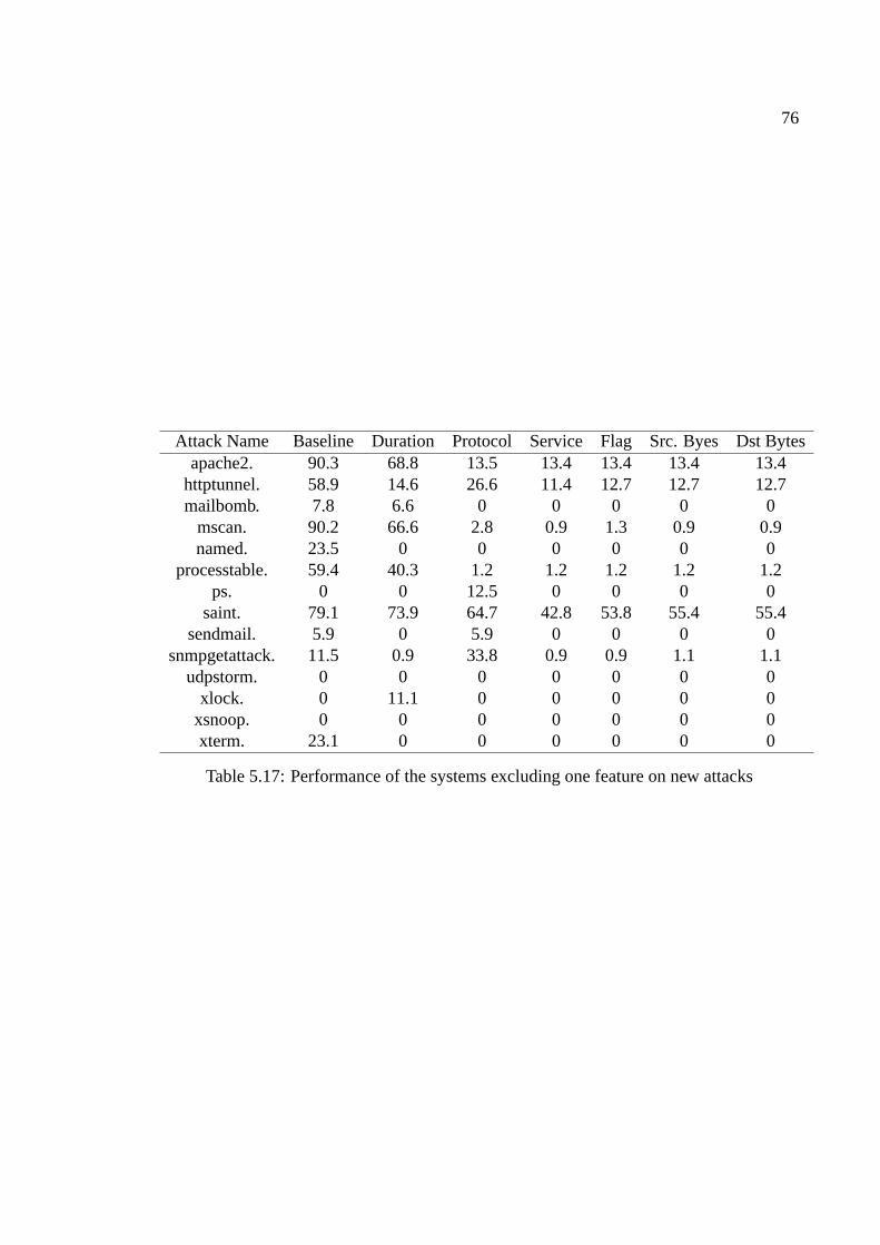
76
Attack Name Baseline Duration Protocol Service Flag Src. Byes Dst Bytesapache2. 90.3 68.8 13.5 13.4 13.4 13.4 13.4
httptunnel. 58.9 14.6 26.6 11.4 12.7 12.7 12.7mailbomb. 7.8 6.6 0 0 0 0 0
mscan. 90.2 66.6 2.8 0.9 1.3 0.9 0.9named. 23.5 0 0 0 0 0 0
processtable. 59.4 40.3 1.2 1.2 1.2 1.2 1.2ps. 0 0 12.5 0 0 0 0
saint. 79.1 73.9 64.7 42.8 53.8 55.4 55.4sendmail. 5.9 0 5.9 0 0 0 0
snmpgetattack. 11.5 0.9 33.8 0.9 0.9 1.1 1.1udpstorm. 0 0 0 0 0 0 0
xlock. 0 11.1 0 0 0 0 0xsnoop. 0 0 0 0 0 0 0xterm. 23.1 0 0 0 0 0 0
Table 5.17: Performance of the systems excluding one feature on new attacks

77
5.4 Comparisons
Table 5.18 provides a summary of recent results from alternative data mining approaches
trained on the KDD-99 dataset and tested using the ’Corrected (Test)’ data [42, 12]. The
details of these systems have been discussed in Chapter 2. In addition, performance of the
the KDD 99 competition winners are given in Table 5.19.
Technique Detection Rate FP RateData-Mining [42] 70-90% 2%Clustering [12] 93% 10%
K-NN [12] 91% 8%SVM [12] 98% 10%
Table 5.18: Recent Results on the KDD benchmark
normal dos probe u2r r2lKDD 99 Winner [3] 99.5 97.1 83.3 13.2 8.4
Table 5.19: Performance of the KDD 99 winner
Detection rates are very similar to those reported for the SOM hierarchy constructed in
our experiments. However, there are actually several additional factors with which these
results need to be interpreted. Firstly, all the data mining approaches are based on all 41
features; the SOM hierarchy only utilizes 6. Secondly, the other systems utilized host based
information, thus providing an advantage when detecting content based attacks [12]. The
SOM hierarchy is a network based IDS, which does not inspect content.

Chapter 6
Conclusions and Future Work
A hierarchical SOM approach to the IDS problem is proposed and demonstrated on the In-
ternational Knowledge Discovery and Data Mining Tools Competition intrusion detection
benchmark [17]. In the proposed three-level hierarchy, each first level map summarizes
one feature. Temporal relations are also encoded on the first level. The second level map
integrates the summaries from the first level maps. Third level maps are built to optimize
performance. Each neuron on second or higher level maps can be considered as a sensor.
Specific attention is given to the representation of connection sequence (time) and the hier-
archical development of abstractions sufficient to permit direct labeling of SOM nodes with
connection type. Other than these two concepts, no additional use ofa priori information
is employed. The proposed system is shown to be capable of learning attack and normal
behavior from the training data and make accurate predictions on the test data, which also
contains new attacks that the system was not trained on.
To understand the effect of the training data set on the overall performance of the learning
system for IDS, three different versions of KDD data set are employed. According to the
version of the dataset, two misuse and one anomaly detection systems are trained. Based
on our results in Tables 5.6, 5.7 and 5.8, using different distributions or percentages of
attack to normal connections does not affect the detection rate of the hierarchical SOM
78

79
architecture. However, it does have an influence on the false positive rate of the detector.
As the nature and ratio of attacks in the training set increase, the false positive rate becomes
more acceptable - indeed with a small decrease in the detection rate.
Building third level maps for those second level neurons that receive counts from attack
and normal connections demonstrate separation between attacks and normal connections.
Although three levels are demonstrated in the hierarchical SOM architecture, more levels
can be added to the hierarchy in the same way that the third level is constructed. If this
hierarchy is deployed in a real world network, when the network behavior changes, for
example due to a new service addition, additional third level maps can be built for sec-
ond level neurons, which starts to produce false alarms for new services, thus tuning the
hierarchy for the new condition without re-training.
To determine the contribution of each of the six basic TCP features, experiments are con-
ducted to assess the influence of each feature by removing the corresponding first level
SOM and re-training second level SOMs. Although in all cases there is a fluctuation,
experiments on the six basic TCP features demonstrated that contributions of the six ba-
sic TCP features to intrusion detection are similar in terms of detection rate (Table 5.15).
However, results show that the protocol feature should be included to reduce the false pos-
itive rate. Moreover, when the service feature is excluded, hierarchical SOM architecture
achieves the lowest false positive rate. In [42], (Bro) flag feature is reported to be most de-
scribing pattern because it is the summary of the connection. Results here, however, show
that exclusion of the flag feature does not dramatically affect the detection or false positive
rates.
In comparison to data mining approaches currently proposed, the approach provides com-
petitive performance whilst utilizing a fraction of the feature set (6 of the 9 ”Basic features
of an Individual TCP connection” and none of the 32 additional higher-level derived fea-
tures). At the same time the SOM hierarchy does not make use of host-based or content-
based information.

80
This work addresses design issues of the hierarchical SOM architecture as well as assessing
the importance of training set biases and contributions of the individual features. However,
there are issues that can be improved such as data collection and summarization issues, fu-
ture work on distributed intrusion detection approach and optimization of SOM algorithm.
Data collection and summarization are very important in case of data driven systems like
the proposed SOM hierarchy. Raw network data of the KDD 99 intrusion detection dataset
is collected from the DARPA 98 simulated test environment and then summarized into con-
nection records with Bro network analyzer. Although collecting raw data from a controlled
environment and then summarizing the data into high-level events is a valid solution, we
also believe that data collection and summarization procedures should be well-defined, thus
can be repeated easily. The KDD 99 intrusion detection data is still the only labeled data,
which enable intrusion detection designers to train and evaluate their systems on and com-
pare the results with other people who employed the same dataset. Since 1999, many new
technologies and protocols have been developed and many new attack types have been de-
vised, therefore this dataset has became outdated. Moreover, intrusion detection designers
should be able to demonstrate that their systems will work for datasets other than DARPA
98 or KDD 99 data. Unfortunately, very little is published about the technical and proce-
dural details of the DARPA intrusion detection environments, which makes it very difficult
to follow their procedures to repeat the data collection. A new test environment is needed
which is well documented and whose methodology is validated [22]. This new system not
only should provide up-to-date data for intrusion detection designers but also should allow
them to examine results in the light of the complete documentation.
The Bro network analyzer, which is used to create KDD 99 dataset, also has some short-
comings. For the KDD 99 dataset, authors of [42] modified the fragment inspection com-
ponent of Bro and extended it to handle ICMP connections. ”Modified Bro” is the net-
work analyzer proposed as the generic component for building intrusion systems. However
”modified Bro” is not publicly available. Our experience with the open source Bro (stable
version 0.7) showed that it needs different policy files to analyze different protocols. Only,

81
TCP and UDP policies are bundled with the open source Bro. Additionally summarization
of the connectionless UDP traffic into connection records is an issue open to discussion.
We agree that generic and publicly available components should be developed to collect
and summarize raw data, which will allow intrusion detection designers to focus on the
intrusion detection component itself. However, currently no such tool is available. De-
signers either choose to utilize KDD 99 dataset, which is outdated, or develop their own
customized network summarizers, which in turn makes comparisons with other systems
difficult. Therefore a generic network analyzer, which is flexible and easy to integrate to
higher intrusion detection components, should be developed.
Distributed intrusion detection is a promising technique, which reduces the amount of mon-
itored data and eliminates boundaries between host based and network based systems. In
distributed intrusion detection, lightweight intrusion detection systems (sensors) are de-
ployed on various locations (computers) of the network. Deployed lightweight sensors
monitor network and/or host activities without consuming as much resource as a ”global”
intrusion detection system does. Collected ”local” data is then sent to a central system to
determine the global state of the network. An example of the distributed intrusion approach
[43] is implemented by using Snort [32] as the sensor component. The proposed hierar-
chical SOM architecture can also be used as the sensor component to develop a distributed
intrusion detection system.
In the KDD 99 dataset, some denial of service attacks such as smurf attack involves sending
many packets to the target host. As a result, the KDD 99 dataset contains many repeating
instances. Training process can be optimized by removing or reducing the repeating in-
stances from the input dataset. However special attention must be given; this might change
the distribution of the input data and the resulting system may suffer in terms of detection
rate.
Another point of optimization is the detection process. In the current hierarchical SOM,
the best matching unit is determined by calculating the distance between the input instance
to all second and possibly third layer neurons. In this case, all the neurons in second and

82
third level maps are used for detection. As indicated in Section 4.1, the SOM places sim-
ilar patterns with consecutive locations. Therefore, representative neurons can be selected
for different neighborhoods, which have the same label. This will reduce the number of
distance calculations between the input instance and the neurons, hence detection time.

Appendix A
KDD 99 Dataset Details
Details of the attack definitions can be found at MIT Lincoln Laboratory web site[30].
Table A.1: Label counts of the KDD 99 datasets
Attack Category Corrected 10 Percent Kdd Whole Kdd
apache2. dos 794 0 0
back. dos 1098 2203 2203
buffer overflow. u2r 22 30 30
ftp write. r2l 3 8 8
guesspasswd. r2l 4367 53 53
httptunnel. r2l 158 0 0
imap. r2l 1 12 12
ipsweep. probe 306 1247 12481
land. dos 9 21 21
loadmodule. u2r 2 9 9
mailbomb. dos 5000 0 0
Continued on next page
83

84
Table A.1: Label counts of the KDD 99 datasets
Attack Category Corrected 10 Percent Kdd Whole Kdd
mscan. probe 1053 0 0
multihop. r2l 18 7 7
named. r2l 17 0 0
neptune. dos 58001 107201 1072017
nmap. probe 84 231 2316
normal. normal 60593 97277 972780
perl. u2r 2 3 3
phf. r2l 2 4 4
pod. dos 87 264 264
portsweep. probe 354 1040 10413
processtable. dos 759 0 0
ps. u2r 16 0 0
rootkit. u2r 13 10 10
saint. probe 736 0 0
satan. probe 1633 1589 15892
sendmail. r2l 17 0 0
smurf. dos 164091 280790 2807886
snmpgetattack. r2l 7741 0 0
snmpguess. r2l 2406 0 0
spy r2l 0 2 2
sqlattack. u2r 2 0 0
teardrop. dos 12 979 979
udpstorm. dos 2 0 0
warezclient. r2l 0 1020 1020
warezmaster. r2l 1602 20 20
worm. r2l 2 0 0
Continued on next page

85
Table A.1: Label counts of the KDD 99 datasets
Attack Category Corrected 10 Percent Kdd Whole Kdd
xlock. r2l 9 0 0
xsnoop. r2l 4 0 0
xterm. u2r 13 0 0
Table A.2: Enumeration of the alphanumeric Protocol feature
Value Assigned0 tcp1 udp2 icmp
Table A.3: Enumeration of the alphanumeric Service feature
Value Assigned
http 0
smtp 1
finger 2
domain u 3
auth 4
telnet 5
ftp 6
eco i 7
ntp u 8
ecr i 9
other 10
private 11
Continued on next page

86
Table A.3: Enumeration of the alphanumeric Service feature
Value Assigned
pop 3 12
ftp data 13
rje 14
time 15
mtp 16
link 17
remote job 18
gopher 19
ssh 20
name 21
whois 22
domain 23
login 24
imap4 25
daytime 26
ctf 27
nntp 28
shell 29
IRC 30
nnsp 31
http 443 32
exec 33
printer 34
efs 35
courier 36
uucp 37
Continued on next page

87
Table A.3: Enumeration of the alphanumeric Service feature
Value Assigned
klogin 38
kshell 39
echo 40
discard 41
systat 42
supdup 43
iso tsap 44
hostnames 45
csnet ns 46
pop 2 47
sunrpc 48
uucp path 49
netbios ns 50
netbios ssn 51
netbios dgm 52
sql net 53
vmnet 54
bgp 55
Z39 50 56
ldap 57
netstat 58
urh i 59
X11 60
urp i 61
pm dump 62
tftp u 63
Continued on next page

88
Table A.3: Enumeration of the alphanumeric Service feature
Value Assigned
tim i 64
red i 65
Table A.4: Enumeration of the Bro Flag feature
Value AssignedSF 0S1 1REJ 2S2 3S0 4S3 5RSTO 6RSTR 7RSTOS0 8OTH 9SH 10

Appendix B
Detailed Detection Rates
Table B.1: Detection rates for each attack type for systems explained in section 5.3.1 and
5.3.2
Attack Category System 1 (Level3) System 1 System 2 System 3
apache2. dos 90.68 90.30 29.22 95.97
back. dos 45.17 50.91 7.19 52.00
buffer overflow. u2r 9.09 13.64 18.18 22.73
ftp write. r2l 0.00 0.00 0.00 33.33
guesspasswd. r2l 9.69 7.95 16.69 13.44
httptunnel. r2l 20.89 58.86 88.61 71.52
imap. r2l 100.00 0.00 100.00 100.00
ipsweep. probe 34.64 25.49 83.01 25.16
land. dos 44.44 100.00 100.00 100.00
loadmodule. u2r 0.00 0.00 0.00 0.00
mailbomb. dos 6.80 7.80 8.00 7.98
mscan. probe 60.87 90.22 92.31 91.74
Continued on next page
89

90
Table B.1: Detection rates for each attack type for systems explained in section 5.3.1
and 5.3.2
Attack Category System 1 (Level3) System 1 System 2 System 3
multihop. r2l 5.56 0.00 16.67 0.00
named. r2l 0.00 23.53 41.18 35.29
neptune. dos 90.89 96.39 97.36 96.93
nmap. probe 53.57 40.48 95.24 85.71
perl. u2r 0.00 0.00 0.00 50.00
phf. r2l 0.00 0.00 50.00 50.00
pod. dos 24.14 6.90 60.92 4.60
portsweep. probe 47.74 51.98 93.79 84.75
processtable. dos 47.56 59.42 77.21 71.94
ps. u2r 0.00 0.00 0.00 6.25
rootkit. u2r 7.69 69.23 53.85 61.54
saint. probe 78.67 79.08 97.42 89.13
satan. probe 69.63 73.67 88.00 76.61
sendmail. r2l 11.76 5.88 29.41 11.76
smurf. dos 99.85 99.85 99.98 99.83
snmpgetattack. r2l 10.28 11.55 23.05 20.10
snmpguess. r2l 2.29 3.20 5.49 7.52
sqlattack. u2r 0.00 50.00 50.00 50.00
teardrop. dos 0.00 16.67 16.67 25.00
udpstorm. dos 0.00 0.00 0.00 0.00
warezmaster. r2l 19.54 27.34 34.14 34.46
worm. r2l 0.00 50.00 50.00 50.00
xlock. r2l 0.00 0.00 11.11 11.11
xsnoop. r2l 0.00 0.00 0.00 0.00
xterm. u2r 30.77 23.08 30.77 38.46

91
Table B.2: Detection rates for each attack type for feature contribution experiments in
Section 5.3.3
Excluded Features
Attack Baseline Duration Protocol Service Flag S.Bytes D.Bytes
apache2. 90.30 68.77 13.48 13.35 13.35 13.35 13.35
back. 50.91 49.00 70.04 30.33 53.37 30.33 30.33
buffer overflow. 13.64 9.09 4.55 0.00 4.55 0.00 0.00
ftp write. 0.00 0.00 0.00 0.00 0.00 0.00 0.00
guess passwd. 7.95 1.08 5.84 0.14 0.27 0.14 0.14
httptunnel. 58.86 14.56 26.58 11.39 12.66 12.66 12.66
imap. 0.00 0.00 0.00 0.00 0.00 0.00 0.00
ipsweep. 25.49 7.84 24.84 15.03 11.11 14.38 14.38
land. 100.00 0.00 0.00 0.00 0.00 0.00 0.00
loadmodule. 0.00 0.00 0.00 0.00 0.00 0.00 0.00
mailbomb. 7.80 6.56 0.00 0.00 0.00 0.00 0.00
mscan. 90.22 66.57 2.75 0.85 1.33 0.85 0.85
multihop. 0.00 11.11 11.11 0.00 0.00 0.00 0.00
named. 23.53 0.00 0.00 0.00 0.00 0.00 0.00
neptune. 96.39 96.20 98.63 90.81 95.49 95.54 95.53
nmap. 40.48 1.19 57.14 1.19 1.19 1.19 1.19
perl. 0.00 0.00 0.00 0.00 0.00 0.00 0.00
phf. 0.00 0.00 0.00 0.00 0.00 0.00 0.00
pod. 6.90 0.00 49.43 1.15 0.00 0.00 0.00
portsweep. 51.98 10.45 22.60 2.26 3.39 2.26 2.26
processtable. 59.42 40.32 1.19 1.19 1.19 1.19 1.19
ps. 0.00 0.00 12.50 0.00 0.00 0.00 0.00
Continued on next page

92
Table B.2: Detection rates for each attack type for feature contribution experiments in
Section 5.3.3
Attack Baseline Duration Protocol Service Flag S.Bytes D.Bytes
rootkit. 69.23 7.69 7.69 0.00 0.00 0.00 0.00
saint. 79.08 73.91 64.67 42.80 53.80 55.43 55.43
satan. 73.67 69.38 85.49 48.99 63.26 63.26 63.26
sendmail. 5.88 0.00 5.88 0.00 0.00 0.00 0.00
smurf. 99.85 99.71 99.85 99.78 99.66 99.77 99.77
snmpgetattack. 11.55 0.87 33.77 0.87 0.92 1.11 1.09
snmpguess. 3.20 0.54 59.98 0.91 0.79 0.83 0.83
sqlattack. 50.00 0.00 0.00 0.00 0.00 0.00 0.00
teardrop. 16.67 0.00 33.33 0.00 0.00 0.00 0.00
udpstorm. 0.00 0.00 0.00 0.00 0.00 0.00 0.00
warezmaster. 27.34 9.30 7.55 0.25 0.69 0.50 0.50
worm. 50.00 0.00 0.00 0.00 0.00 0.00 0.00
xlock. 0.00 11.11 0.00 0.00 0.00 0.00 0.00
xsnoop. 0.00 0.00 0.00 0.00 0.00 0.00 0.00
xterm. 23.08 0.00 0.00 0.00 0.00 0.00 0.00

Appendix C
U-Matrix Displays of the 2nd Level
SOMs in Section 5.3.1
Figure C.1: U-Matrix of the second level map for the 10% KDD dataset
93

94
Figure C.2: U-Matrix of the second level map for the normal only10% KDD dataset
Figure C.3: U-Matrix of the second level map for the 50/50 dataset

Appendix D
U-Matrix and Labels of the 2nd Level
SOMs in Section 5.3.3
Black : Attack Gray : Unlabeled White : Normal
Figure D.1: U-matrix and labels for the baseline 36 dimensional second level map (System1)
95

96
Black : Attack Gray : Unlabeled White : Normal
Figure D.2: U-matrix and labels for the duration excluded second level map
Black : Attack Gray : Unlabeled White : Normal
Figure D.3: U-matrix and labels for the protocol excluded second level map

97
Black : Attack Gray : Unlabeled White : Normal
Figure D.4: U-matrix and labels for the service excluded second level map
Black : Attack Gray : Unlabeled White : Normal
Figure D.5: U-matrix and labels for the flag excluded second level map

98
Black : Attack Gray : Unlabeled White : Normal
Figure D.6: U-matrix and labels for the source bytes excluded second level map
Black : Attack Gray : Unlabeled White : Normal
Figure D.7: U-matrix and labels for the destination bytes excluded second level map

Bibliography
[1] Miheev V.and Vopilov A. and Shabalin I. The MP13 Approach to the KDD’99 Clas-sifier Learning Contest.SIGKDD Explorations, 1(2):76–77, 2000.
[2] Ultsch A. and Siemon H. Kohonen’s self-organizing feature maps for exploratory dataanalysis. InProceedings of the International Neural Network Conference (INNC’90),Dordrecht, Netherlands, pages 305–308. Kluwer, 1990.
[3] Pfahringer B. Winning the KDD99 Classification Cup: Bagged Boosting.SIGKDDExplorations, 1(2):65–66, 2000.
[4] Rhodes B.C., Mahaffey J.A., and Cannady J.D. Multiple Self-Organizing Maps forIntrusion Detection. InProceedings of 23rd National Information Systems SecurityConference, 2000.
[5] Nguyen B.V. Self Organizing Map (SOM) for Anomaly Detection. Ohio UniversitySchool of Electrical Engineering and Computer Science CS680 Technical Report,Spring 2002.
[6] Elkan C. Results of the KDD’99 Classifier Learning. InACM SIGKDD Explorations,volume 1, pages 63–64, 2000.
[7] Jirapummin C., Wattanapongsakorn N., and Kanthamanon P. Hybrid neural networksfor intrusion detection system. InProceedings of The 2002 International TechnicalConference On Circuits/Systems, Computers and Communications, 2002.
[8] J. Cannady. Artificial neural networks for misuse detection. InProceedings of the1998 National Information Systems Security Conference (NISSC’98) October 5-81998. Arlington, VA., pages 443–456, 1998.
[9] CERT/CCc©. Identifying Tools That Aid in Detecting Signs of Intrusion. Web site,Jan 2001.http://www.cert.org/security-improvement/implementations/i042.07.html .
99

100
[10] CERT/CCc©. Incident Statistics 1988-2002. Web Site, 2002.http://www.cert.org/stats/cert stats.html .
[11] Denning D.E. An Intrusion Detection Model. InIEEE Transactions on SoftwareEngineering, volume SE-13, pages 222–232, Feb. 1987.
[12] Eskin E., Arnold A., Prerau M., Portnoy L., and Stolfo S. A Geometric Frameworkfor Unsupervised Anomaly Detection: Detecting intrusions in unlabeled data. InD. Barbara and S. Jajodia, editors,Applications of Data Mining in Computer Security.Kluwer, 2002. ISBN 1-4020-7054-3, 2002.
[13] Grinstein G. Information Exploration Shootout Project and Benchmark Data Sets:Evaluating how Visualization does in Analyzing Real-World Data Analysis Problems.In Proceedings of IEEE Visualization ’97, pages 511–513, Oct. 1997.
[14] Kayacik G. and Zincir-Heywood N. A Case Study Of Three Open Source SecurityManagement Tools. InProceedings of International Symposium on Integrated Net-work Management, 2003.
[15] Kayacik G., Zincir-Heywood N., and Heywood M. On the Capability of an SOMbased Intrusion Detection System. InProceedings of International Joint Conferenceon Neural Networks, 2003.
[16] MIT Lincoln Laboratory Information Systems Technology Group.The 1998 Intrusion Detection Off-line Evaluation Plan, March 1998.http://www.ll.mit.edu/IST/ideval/docs/1998/id98-eval-ll.txt .
[17] S. Hettich and S. D Bay. The UCI KDD Archive. Irvine, CA: Univer-sity of California, Department of Information and Computer Science., 1999.http://kdd.ics.uci.edu .
[18] Hoglund A.J. and Hatonen K and Sorvari A.S. A Computer Host-based User AnomalyDetection System using Self-Organizing Map. InProceedings of the IEEE-INNS-ENNS International Joint Conference on Neural Networks, volume 5, pages 411–416,2000.
[19] Levin I. KDD-99 Classifier Learning Contest: LLSoft’s Results Overview.SIGKDDExplorations, 1(2):67–75, 2000.
[20] Witten I.H. and Frank E.Data Mining: Practical Machine Learning Tools and Tech-niques with Java Implementations. Morgan Kaufmann, 2002.
[21] Cannady J. Next Generation Intrusion Detection: Autonomous Reinforcement Learn-ing of Network Attacks. InProceedings of 23rd National Information Systems Secu-rity Conference, 2000.

101
[22] McHugh J. Testing Intrusion detection systems: a critique of the 1998 and 1999DARPA intrusion detection system evaluations as performed by Lincoln Labora-tory. ACM Transactions on Information and System Security (TISSEC), 3(4):262–294,2000.
[23] Vesanto J. Data Mining Techniques Based on the Self-Organizing Map. Master’sthesis, Helsinki University of Technology, May 1997.
[24] Albus J.S. A New Approach to Control: The Cerebellar model Articulation Controller(CMAC). Transactions of ASME, Sep. 1975.
[25] Labib K. and Vemuri R. NSOM: A Real-Time Network-Based Intrusion DetectionUsing Self-Organizing Maps.Networks and Security, 21(1), Oct. 2002.
[26] Takeda K. and Takefuji Y. Pakemon - A Rule Based Network Intrusion Detection Sys-tem. In International Journal of Knowledge-Based Intelligent Engineering Systems,volume 5, pages 240–246, Oct. 2001.
[27] R. A. Kemmerer and G. Vigna. Intrusion detection: A brief history and overview.IEEE Security and Privacy, April 2002.
[28] Girardin L. An Eye on Network Intruder-Administrator Shootouts. InProceedings ofthe Workshop on Intrusion Detection and Network Monitoring, Apr. 1999.
[29] MIT Lincoln Laboratory. DARPA 99 Intru-sion Detection Data Set Attack Documentation.http://www.ll.mit.edu/IST/ideval/docs/1999/attackDB.html .
[30] MIT Lincoln Laboratory. Intrusion Detection Datasets.http://www.ll.mit.edu/IST/ideval/data/data index.html .
[31] Bing M. and Turner A. TCPReplay traffic replay utility. Web site.http://tcpreplay.sourceforge.net/ .
[32] Roesch M. Snort - Lightweight Intrusion Detection for Networks. In13th SystemsAdministration Conference, Proceedings of LISA, 1999.
[33] Joshi M.V., Agarwal R.C., and Kumar V. Mining needle in a haystack: classifyingrare classes via two-phase rule induction.SIGMOD Record (ACM Special InterestGroup on Management of Data), 30(2):91–102, 2001.
[34] University of California Department of Information and Computer Sci-ence. Kdd cup 99 intrusion detection dataset task description, 1999.http://kdd.ics.uci.edu/databases/kddcup99/task.html .

102
[35] Laboratory of Computer and Information Science Neural Networks Re-search Centre. Software Packages from Helsinki University of Technology.http://www.cis.hut.fi/research/software.shtml .
[36] Lichodzijewski P., Zincir-Heywood N., and Heywood M. Host-Based Intrusion De-tection Using Self Organizing Maps. InProceedings of IEEE International JointConference on Neural Networks, pages 1714–1719, 2002.
[37] Lippmann R., Fried D., Graf I., Haines J., Kendall K., McClung D., Weber S., WebsterS., Wyschogrod S., Cunningham R., and Zissman M. Evaluating Intrusion DetectionSystems: The 1998 DARPA Off-line Intrusion Detection Evaluation. InProceedingsof the DARPA Information Survivability Conference and Exposition, Los Alamitos,CA, 2000. IEEE Computer Society Press.
[38] Chiu S.L. Fuzzy model identification based on cluster estimation. InJournal ofIntelligent and Fuzzy Systems, number 2, pages 267–278, 1994.
[39] Cisco Systems. Cisco IOS Firewall Intrusion Detection System Documentation. 2003.http://www.cisco.com/univercd/cc/td/doc/product/software/ios120/120newft/120t/120t5/iosfw2/ios ids.htm .
[40] Kohonen T.Self Organizing Maps. Springer, third edition, 2001.
[41] Paxson V. Bro: a system for detecting network intruders in real-time.ComputerNetworks (Amsterdam, Netherlands: 1999), 31(23–24):2435–2463, 1999.
[42] Lee W. and Stolfo S. A Framework for Constructing Features and Models for Intru-sion Detection Systems.Information and System Security, 3(4):227–261, 2000.
[43] Fyodor Y. ‘Snortnet’ - A Distributed Intrusion Detection System.