hidden markov models and their mixtures - scarlet
TRANSCRIPT

Universit�e catholique de Louvain
Facult�e des sciences { D�epartement de math�ematiques
Hidden Markov Models and Their Mixtures
Rapport pr�esent�e en vue de l'obtention du
Diplome d'�etudes approfondies en math�ematiques par :
Christophe Couvreur
Membres du jury:
Prof. Jean-Marie Rolin (promoteur)
Prof. Jacques Teghem Jr, FPMs
Prof. Pierre van Moerbeke
{ 1996 {

Abstract
Hidden Markov Models and Their Mixtures
by
Christophe Couvreur
Diplome d'�etudes approfondies en math�ematiques
Facult�e des sciences { D�epartement de math�ematiques, Universit�e catholique de
Louvain
Prof. Jean-Marie Rolin, Advisor
Hidden Markov models (HMMs) form a class of stochastic processes which have been applied
successfully to a wide variety of practical problems. Hidden Markov models are based on
an unobserved (or hidden) discrete Markov chain fXng which describes the evolution of the
state of a system. Given a realization fxng of the state process, the observed variables fYngare conditionally independent, with the distribution of each Yn function of the corresponding
state xn only.
Solutions to the three basic hidden Markov modeling problems are presented: compu-
tation of the likelihood of a realization yN0 = (y0; y2; : : : ; yN ) given a model, estimation of
the corresponding unobserved state sequence XN0 = (X0;X1; : : : ;XN ), and computation of
the maximum likelihood estimate of the HMM parameters. A review of the HMM litera-
ture covering a wide range of applications is also provided. Inference issues for HMMs are
discussed, including the description of the properties of the maximum likelihood estimates
and a presentation of other estimation methodologies. Particular attention is devoted to
the classi�cation of HMMs (multiple point hypotheses testing). The new concept of mix-
ture of HMMs is introduced. Various estimation and classi�cation problems for mixtures of
HMMs are investigated, with special care taken of the \decomposition of mixtures" question.
Some preliminary numerical results are presented. Finally, directions for future research are
proposed.

iii
To Fran�coise.

iv
Contents
List of Figures viii
List of Tables x
1 Introduction 1
I Review of Hidden Markov Models 7
2 De�nition of Hidden Markov Models 8
2.1 De�nition . . . . . . . . . . . . . . . . . . . . . . . . . . . . . . . . . . . . . . 8
2.1.1 Discrete Hidden Markov Models . . . . . . . . . . . . . . . . . . . . . 10
2.1.2 Continuous Hidden Markov Models . . . . . . . . . . . . . . . . . . . . 12
2.1.3 Markov-Modulated Time Series and HMMs . . . . . . . . . . . . . . . 13
2.2 Variants and Terminology . . . . . . . . . . . . . . . . . . . . . . . . . . . . . 15
2.2.1 Types of HMMs . . . . . . . . . . . . . . . . . . . . . . . . . . . . . . 15
2.2.1.1 Ergodic HMMs . . . . . . . . . . . . . . . . . . . . . . . . . . 15
2.2.1.2 Stationary HMMs . . . . . . . . . . . . . . . . . . . . . . . . 16
2.2.1.3 Left-Right HMMs . . . . . . . . . . . . . . . . . . . . . . . . 17
2.2.2 Variable Duration HMMs . . . . . . . . . . . . . . . . . . . . . . . . . 18
2.2.3 Exogenous Inputs HMMs . . . . . . . . . . . . . . . . . . . . . . . . . 19
3 Computations with Hidden Markov Models 21
3.1 Computation of the Likelihood . . . . . . . . . . . . . . . . . . . . . . . . . . 22
3.1.1 The Forward Algorithm . . . . . . . . . . . . . . . . . . . . . . . . . . 22
3.1.2 The Backward Algorithm . . . . . . . . . . . . . . . . . . . . . . . . . 25
3.1.3 Matrix Formulation . . . . . . . . . . . . . . . . . . . . . . . . . . . . 25
3.2 Computation of the Most Likely Sequence of States . . . . . . . . . . . . . . . 26
3.3 Computation of the Maximum Likelihood Estimate of the Model Parameters 29
3.3.1 Maximum Likelihood Estimator . . . . . . . . . . . . . . . . . . . . . 29
3.3.2 The Baum-Welsh Algorithm . . . . . . . . . . . . . . . . . . . . . . . . 29
3.3.3 Examples . . . . . . . . . . . . . . . . . . . . . . . . . . . . . . . . . . 33
3.3.3.1 Non-Parametric Discrete HMM . . . . . . . . . . . . . . . . . 33
3.3.3.2 Binomial Discrete HMM . . . . . . . . . . . . . . . . . . . . 34
3.3.3.3 Poisson Discrete HMM . . . . . . . . . . . . . . . . . . . . . 34
3.3.3.4 Gaussian Continuous HMM . . . . . . . . . . . . . . . . . . . 34
3.3.3.5 Mixture of Gaussians Continuous HMM . . . . . . . . . . . . 35
3.3.4 Convergence Properties of the Baum-Welsh Algorithm . . . . . . . . . 36

v
3.3.5 Direct Maximization of the Likelihood . . . . . . . . . . . . . . . . . . 38
3.3.6 Multiple Observation Sequences . . . . . . . . . . . . . . . . . . . . . . 38
3.4 Practical Implementation Issues . . . . . . . . . . . . . . . . . . . . . . . . . . 39
3.4.1 Thresholding . . . . . . . . . . . . . . . . . . . . . . . . . . . . . . . . 39
3.4.2 Scaling . . . . . . . . . . . . . . . . . . . . . . . . . . . . . . . . . . . 40
3.5 Recursive Computations . . . . . . . . . . . . . . . . . . . . . . . . . . . . . . 40
4 Applications of Hidden Markov Models 42
4.1 Connections with Other Models . . . . . . . . . . . . . . . . . . . . . . . . . . 42
4.1.1 State-Space Models . . . . . . . . . . . . . . . . . . . . . . . . . . . . 42
4.1.2 Mixture Models and Switching Regressions . . . . . . . . . . . . . . . 43
4.1.3 Hidden Markov Random Fields . . . . . . . . . . . . . . . . . . . . . . 44
4.1.4 Neural Networks . . . . . . . . . . . . . . . . . . . . . . . . . . . . . . 45
4.1.5 Probabilistic Networks . . . . . . . . . . . . . . . . . . . . . . . . . . . 45
4.2 Applications . . . . . . . . . . . . . . . . . . . . . . . . . . . . . . . . . . . . . 46
4.2.1 Speech Processing . . . . . . . . . . . . . . . . . . . . . . . . . . . . . 47
4.2.2 Image Processing . . . . . . . . . . . . . . . . . . . . . . . . . . . . . . 48
4.2.3 Sonar Signal Processing . . . . . . . . . . . . . . . . . . . . . . . . . . 48
4.2.4 Automatic Fault Detection and Monitoring . . . . . . . . . . . . . . . 48
4.2.5 Information Theory . . . . . . . . . . . . . . . . . . . . . . . . . . . . 49
4.2.6 Communication . . . . . . . . . . . . . . . . . . . . . . . . . . . . . . . 49
4.2.7 Theory of Optimal Estimation And Control . . . . . . . . . . . . . . . 49
4.2.8 Non-Stationary Time Series Analysis . . . . . . . . . . . . . . . . . . . 50
4.2.9 Biomedical applications . . . . . . . . . . . . . . . . . . . . . . . . . . 51
4.2.10 Epidemiology and Biometrics . . . . . . . . . . . . . . . . . . . . . . . 51
4.2.11 Other Applications . . . . . . . . . . . . . . . . . . . . . . . . . . . . . 51
4.3 The Role of HMMs as Statistical Models . . . . . . . . . . . . . . . . . . . . . 52
5 Inference for Hidden Markov Models 53
5.1 Hypothesis Testing . . . . . . . . . . . . . . . . . . . . . . . . . . . . . . . . . 53
5.1.1 The Classi�cation Problem . . . . . . . . . . . . . . . . . . . . . . . . 53
5.1.2 Other Statistical Tests for HMMs . . . . . . . . . . . . . . . . . . . . . 55
5.1.2.1 Likelihood Ratio Tests for Simple Hypotheses . . . . . . . . 55
5.1.2.2 Tests for Composite Hypotheses . . . . . . . . . . . . . . . . 56
5.2 Asymptotic Properties of HMMs . . . . . . . . . . . . . . . . . . . . . . . . . 57
5.2.1 Identi�ability of HMMs . . . . . . . . . . . . . . . . . . . . . . . . . . 57
5.2.2 The Shannon-McMillan-Breinman Theorem for HMMs . . . . . . . . . 58
5.2.3 The Kullback-Leibler Divergence for HMMs . . . . . . . . . . . . . . . 58
5.2.4 Maximum Likelihood Estimation . . . . . . . . . . . . . . . . . . . . . 59
5.2.4.1 Consistency of the MLE . . . . . . . . . . . . . . . . . . . . . 59
5.2.4.2 Asymptotic Normality of the MLE . . . . . . . . . . . . . . . 60
5.2.4.3 The Multiple Observation Sequence Case . . . . . . . . . . . 60
5.2.5 Viterbi Approximation of the Likelihood . . . . . . . . . . . . . . . . . 61
5.2.6 Maximum Split-Data Likelihood Estimates . . . . . . . . . . . . . . . 64
5.2.7 Bayesian Estimation . . . . . . . . . . . . . . . . . . . . . . . . . . . . 64
5.2.8 Alternative Estimation Approaches . . . . . . . . . . . . . . . . . . . . 66
5.2.8.1 Discriminative Training and Minimum Empirical Error Rate
Estimator . . . . . . . . . . . . . . . . . . . . . . . . . . . . . 67

vi
5.2.8.2 Maximum Mutual Information Estimator . . . . . . . . . . . 68
5.2.8.3 Minimum Discrimination Information Estimator . . . . . . . 69
5.2.9 Selection of the Structural Parameters of a HMM . . . . . . . . . . . . 70
5.2.9.1 Empirical Approach . . . . . . . . . . . . . . . . . . . . . . . 70
5.2.9.2 Penalized Likelihood Approach . . . . . . . . . . . . . . . . . 70
5.2.9.3 Information Theoretic Approach . . . . . . . . . . . . . . . . 73
II Decomposition of Mixtures of Hidden Markov Models 74
6 Mixtures of Hidden Markov Models 75
6.1 Introduction . . . . . . . . . . . . . . . . . . . . . . . . . . . . . . . . . . . . . 75
6.2 De�nition . . . . . . . . . . . . . . . . . . . . . . . . . . . . . . . . . . . . . . 75
6.3 Relation with Hidden Markov Models . . . . . . . . . . . . . . . . . . . . . . 77
6.4 Types of MHMMs . . . . . . . . . . . . . . . . . . . . . . . . . . . . . . . . . 82
6.4.1 Mixtures of Discrete HMMs . . . . . . . . . . . . . . . . . . . . . . . . 82
6.4.2 Mixtures of Continuous HMMs . . . . . . . . . . . . . . . . . . . . . . 83
6.5 Computation and Inference for Mixtures of HMMs . . . . . . . . . . . . . . . 85
6.5.1 Algorithms for Computations with MHMMs . . . . . . . . . . . . . . . 85
6.5.2 Filtering of MHMMs . . . . . . . . . . . . . . . . . . . . . . . . . . . . 86
6.5.2.1 MMSE Estimator . . . . . . . . . . . . . . . . . . . . . . . . 86
6.5.2.2 MAP Estimator . . . . . . . . . . . . . . . . . . . . . . . . . 87
6.5.3 Decomposition of MHMMs . . . . . . . . . . . . . . . . . . . . . . . . 88
6.6 Applications and Related Models . . . . . . . . . . . . . . . . . . . . . . . . . 90
6.6.1 Environmental Sound Recognition . . . . . . . . . . . . . . . . . . . . 90
6.6.2 Speech Plus Noise HMMs . . . . . . . . . . . . . . . . . . . . . . . . . 92
6.6.2.1 Speech Enhancement . . . . . . . . . . . . . . . . . . . . . . 92
6.6.2.2 Noisy Speech Recognition . . . . . . . . . . . . . . . . . . . . 92
6.6.3 Multiple Object Tracking . . . . . . . . . . . . . . . . . . . . . . . . . 93
7 Decomposition of Mixtures of Discrete Hidden Markov Models 94
7.1 Problem Formulation . . . . . . . . . . . . . . . . . . . . . . . . . . . . . . . . 94
7.2 Optimal Solution: The Bayes Classi�er . . . . . . . . . . . . . . . . . . . . . . 97
7.3 Sub-Optimal Solutions . . . . . . . . . . . . . . . . . . . . . . . . . . . . . . . 99
7.3.1 A Simpli�ed Decision Statistic . . . . . . . . . . . . . . . . . . . . . . 99
7.3.2 Sub-Optimal Search Strategies . . . . . . . . . . . . . . . . . . . . . . 101
7.4 Preliminary Experiments . . . . . . . . . . . . . . . . . . . . . . . . . . . . . 102
7.4.1 Dictionary of HMM Components . . . . . . . . . . . . . . . . . . . . . 102
7.4.2 Modeling of the Pre-Processor . . . . . . . . . . . . . . . . . . . . . . 103
7.4.3 Numerical Results . . . . . . . . . . . . . . . . . . . . . . . . . . . . . 104
8 Decomposition of Mixtures of Continuous Hidden Markov Models 107
8.1 Problem Formulation . . . . . . . . . . . . . . . . . . . . . . . . . . . . . . . . 107
8.2 Proposed Solutions . . . . . . . . . . . . . . . . . . . . . . . . . . . . . . . . . 109
8.2.1 Penalized Likelihood Method . . . . . . . . . . . . . . . . . . . . . . . 109
8.2.2 �2 Test Method . . . . . . . . . . . . . . . . . . . . . . . . . . . . . . . 110
8.2.3 Likelihood Maximization . . . . . . . . . . . . . . . . . . . . . . . . . 112
9 Conclusion and Directions for Future Research 114

vii
A Discrete Markov Chains 116
A.1 De�nition . . . . . . . . . . . . . . . . . . . . . . . . . . . . . . . . . . . . . . 116
A.2 Properties of Markov Chains . . . . . . . . . . . . . . . . . . . . . . . . . . . 117
A.2.1 Transition Probability Matrices of a Markov Chain . . . . . . . . . . . 117
A.2.2 Classi�cation of State of a Markov Chain . . . . . . . . . . . . . . . . 118
A.2.3 Limit Behavior of a Markov Chain . . . . . . . . . . . . . . . . . . . . 119
B The EM Algorithm 120
B.1 Introduction . . . . . . . . . . . . . . . . . . . . . . . . . . . . . . . . . . . . . 120
B.2 The EM Algorithm . . . . . . . . . . . . . . . . . . . . . . . . . . . . . . . . . 121
B.2.1 Incomplete Data Problems . . . . . . . . . . . . . . . . . . . . . . . . 121
B.2.2 The EM Algorithm . . . . . . . . . . . . . . . . . . . . . . . . . . . . . 121
B.2.3 A Notional Example . . . . . . . . . . . . . . . . . . . . . . . . . . . . 122
B.3 Practical Applications . . . . . . . . . . . . . . . . . . . . . . . . . . . . . . . 124
B.3.1 Motivation . . . . . . . . . . . . . . . . . . . . . . . . . . . . . . . . . 124
B.3.2 Examples of Applications . . . . . . . . . . . . . . . . . . . . . . . . . 125
B.3.2.1 Mixture Densities . . . . . . . . . . . . . . . . . . . . . . . . 125
B.3.2.2 PET Tomography . . . . . . . . . . . . . . . . . . . . . . . . 125
B.3.2.3 System Identi�cation . . . . . . . . . . . . . . . . . . . . . . 126
B.4 Convergence Properties . . . . . . . . . . . . . . . . . . . . . . . . . . . . . . 126
B.4.1 Monotonous Increase of the Likelihood . . . . . . . . . . . . . . . . . . 126
B.4.2 Convergence to a Local Maxima . . . . . . . . . . . . . . . . . . . . . 127
B.4.3 Speed of Convergence . . . . . . . . . . . . . . . . . . . . . . . . . . . 128
B.5 Variants of the EM Algorithm . . . . . . . . . . . . . . . . . . . . . . . . . . . 128
B.5.1 Acceleration of the Algorithm . . . . . . . . . . . . . . . . . . . . . . . 128
B.5.2 Approximation of the E or M Step . . . . . . . . . . . . . . . . . . . . 128
B.5.3 Penalized Likelihood Estimation . . . . . . . . . . . . . . . . . . . . . 128
B.6 Concluding Remarks . . . . . . . . . . . . . . . . . . . . . . . . . . . . . . . . 129
Bibliography 131
viii
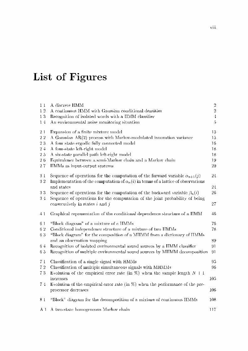
List of Figures
1.1 A discrete HMM. . . . . . . . . . . . . . . . . . . . . . . . . . . . . . . . . . . 2
1.2 A continuous HMM with Gaussian conditional densities. . . . . . . . . . . . . 2
1.3 Recognition of isolated words with a HMM classi�er. . . . . . . . . . . . . . . 4
1.4 An environmental noise monitoring situation. . . . . . . . . . . . . . . . . . . 5
2.1 Expansion of a �nite mixture model. . . . . . . . . . . . . . . . . . . . . . . . 13
2.2 A Gaussian AR(2) process with Markov-modulated innovation variance. . . . 15
2.3 A four-state ergodic fully connected model. . . . . . . . . . . . . . . . . . . . 16
2.4 A four-state left-right model. . . . . . . . . . . . . . . . . . . . . . . . . . . . 18
2.5 A six-state parallel path left-right model. . . . . . . . . . . . . . . . . . . . . 18
2.6 Equivalence between a semi-Markov chain and a Markov chain. . . . . . . . . 19
2.7 HMMs as input-output systems. . . . . . . . . . . . . . . . . . . . . . . . . . 20
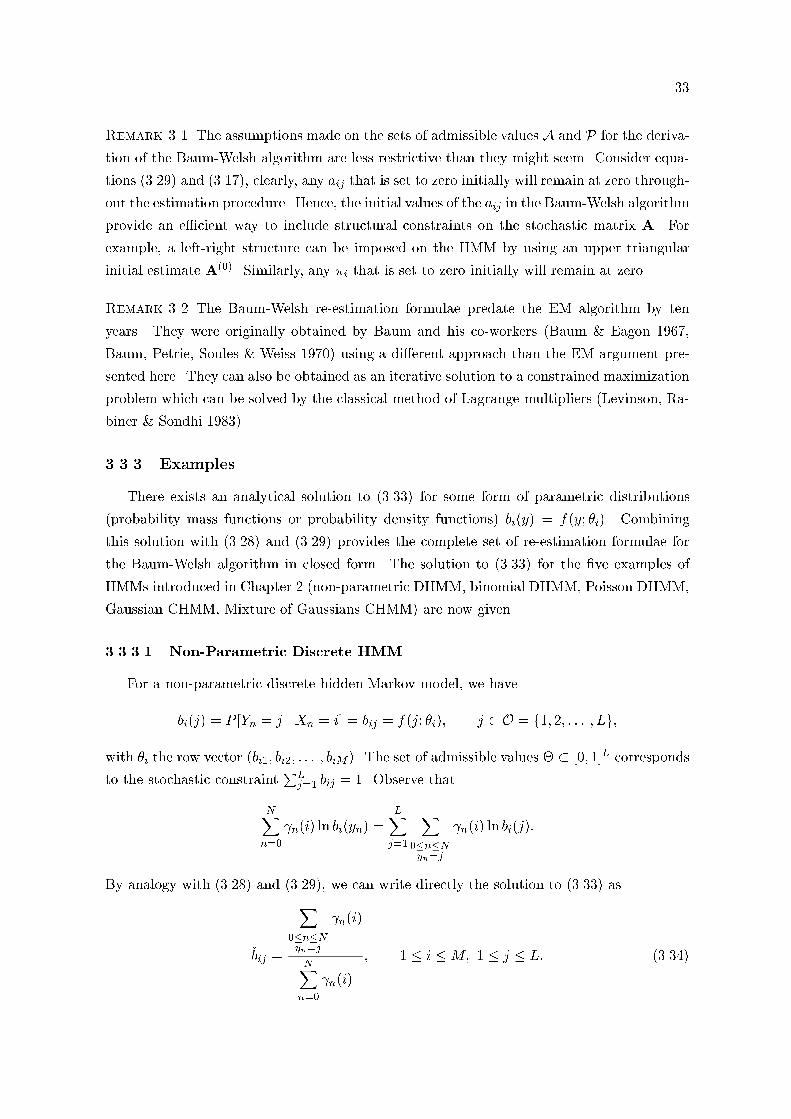
3.1 Sequence of operations for the computation of the forward variable �n+1(j). . 24
3.2 Implementation of the computation of �n(i) in terms of a lattice of observations
and states. . . . . . . . . . . . . . . . . . . . . . . . . . . . . . . . . . . . . . . 24
3.3 Sequence of operations for the computation of the backward variable �n(i). . 26
3.4 Sequence of operations for the computation of the joint probability of being
consecutively in states i and j. . . . . . . . . . . . . . . . . . . . . . . . . . . 27
4.1 Graphical representation of the conditional dependence structure of a HMM. 46
6.1 \Block diagram" of a mixture of c HMMs. . . . . . . . . . . . . . . . . . . . . 76
6.2 Conditional independence structure of a mixture of two HMMs. . . . . . . . . 78
6.3 \Block diagram" for the composition of a MHMM from a dictionary of HMMs
and an observation mapping. . . . . . . . . . . . . . . . . . . . . . . . . . . . 89
6.4 Recognition of isolated environmental sound sources by a HMM classi�er. . . 91
6.5 Recognition of multiple environmental sound sources by MHMM decomposition. 91
7.1 Classi�cation of a single signal with HMMs. . . . . . . . . . . . . . . . . . . . 95
7.2 Classi�cation of multiple simultaneous signals with MHMMs. . . . . . . . . . 96
7.3 Evolution of the empirical error rate (in %) when the sample length N + 1
increases. . . . . . . . . . . . . . . . . . . . . . . . . . . . . . . . . . . . . . . 105
7.4 Evolution of the empirical error rate (in %) when the performance of the pre-
processor decreases. . . . . . . . . . . . . . . . . . . . . . . . . . . . . . . . . 106
8.1 \Block" diagram for the decomposition of a mixture of continuous HMMs. . . 108
A.1 A two-state homogeneous Markov chain. . . . . . . . . . . . . . . . . . . . . . 117

ix
A.2 An example of Markov chain. . . . . . . . . . . . . . . . . . . . . . . . . . . . 119

x
List of Tables
2.1 De�nition of a HMM. . . . . . . . . . . . . . . . . . . . . . . . . . . . . . . . 14
3.1 The forward algorithm. . . . . . . . . . . . . . . . . . . . . . . . . . . . . . . 23
3.2 The backward algorithm. . . . . . . . . . . . . . . . . . . . . . . . . . . . . . 25
3.3 The Viterbi algorithm. . . . . . . . . . . . . . . . . . . . . . . . . . . . . . . . 28
3.4 The Baum-Welsh algorithm. . . . . . . . . . . . . . . . . . . . . . . . . . . . . 32
5.1 The segmental k-means algorithm. . . . . . . . . . . . . . . . . . . . . . . . . 63
6.1 The forward algorithm for MHMMs. . . . . . . . . . . . . . . . . . . . . . . . 85

xi
Acknowledgements
This work would not have been possible without my advisor, Prof. Jean-Marie Rolin of
the Institute of Statistics of Universit�e catholique de Louvain. I would like to thank him here
for his assistance and patience.
I would also like to thank Prof. Jacques Teghem from Facult�e Polytechnique de Mons and
Prof. van Moerbeke from Universit�e catholique de Louvain for agreeing to be on the reading
committee.
I am grateful to the Belgian National Fund for Scienti�c Research (F.N.R.S.) and to
Belgacom for their �nancial support.
In addition, I wish to express my gratitude to the Service de Physique G�en�erale and the
Service de Th�eorie des Circuit et de Traitement du Signal of Facult�e Polytechnique de Mons
for their logistic support. A special thanks goes to Vincent Fontaine for his help with the
simulations of Chapter 7.
Finally, a very special thanks to my wife-to-be Fran�coise for coping with my long o�ce
hours.

1
Chapter 1
Introduction
Hidden Markov models or HMMs form a large and useful class of stochastic processes.
They were originally introduced by Baum and Petrie in (Baum & Petrie 1966). Since then
they have become important in a wide variety of applications including, �rst and foremost,
automatic speech recognition (see (Rabiner 1989) for an introduction and survey), biometrics
(Albert 1991, Leroux 1992b), econometrics (Hamilton 1989, Hamilton 1990), molecular biol-
ogy (Krogh, Brown, Mian, Sjolander & Haussler 1994), fault detection (Smyth 1994a, Smyth
1994b, Ayanoglu 1992), among many others.
Hidden Markov models are based on an unobserved (or hidden) discrete Markov chain
fXng which describes the evolution of the state of a system. Given a realization of the state
process fxng, the observed variables fYng are conditionally independent, with the distributionof each Yn depending on the corresponding state xn only. The random variables Yn can
take their values in a discrete or continuous space. If the variables Yn are discrete, the
model is called a discrete hidden Markov model (DHMM). Figure 1.1 illustrates a discrete
hidden Markov model on an \urn and ball" example. The hidden two-state Markov chain is
represented as a graph, with aij denoting the transition probability from state i to state j. At
each time instant n, an urn is selected according to the evolution of the Markov chain, and a
ball is drawn from the selected urn with replacement. The sequence of black or white valued
variables formed by the color of the balls drawn obeys a discrete HMM. If the variables Yn
are continuous, the model is called a continuous hidden Markov model (CHMM). In this case,
the observed variables Yn have conditional probability distribution functions which depends
on the states xn. Often, a parametric family is used for the conditional distributions; the
HMM can then be viewed as a parametric model whose parameters vary with the state of
the Markov chain. An example of CHMM with Gaussian conditional densities for Yn is
represented in Figure 1.2. At each time instant, a parametric (Gaussian) model is selected
according to the state of the hidden Markov chain, and an observation is drawn with that
distribution. The resulting sequence of observation obeys a continuous HMM.
Following J. D. Fergusson (Rabiner 1989), we can state the three basic problems that

2
1 2
-a12
�a21
-a11 -
a22
Figure 1.1: A discrete HMM.
-
6
-
6
�1
-� �1
�2
-� �2
1 2
-a12
�a21
-a11 -
a22
Figure 1.2: A continuous HMM with Gaussian conditional densities.

3
must be solved �rst for hidden Markov models to be useful in real-world applications:
1. Given an observation sequence (y0; y1; : : : ; yN ) and a HMM, how do we e�ciently com-
pute the likelihood of the observation sequence?
2. Given an observation sequence (y0; y1; : : : ; yN ) and a HMM, how do we estimate the
corresponding unobserved state sequence ?
3. How do we estimate the model (Markov chain parameters and conditional distributions)
from �nite length realizations of fYng? Particularly, how do we compute the maximum-
likelihood estimate?
As we will see shortly, it is possible to use dynamic programming methods to solve problems 1
and 2 in linear time, and a variant of the EM algorithm can be applied to solve e�ciently
problem 3.
Once the three fundamental questions have been answered, it becomes possible to address
inference issues involving HMMs. The statistical properties of HMMs and of the estimates of
their parameters can be obtained, and hypothesis testing methodologies can be developed. Of
particular interest to us is the classi�cation problem: given a family of possible hiddenMarkov
models, how do we classify an observation sequence fy0; y1; : : : ; yng such as to minimize the
probability of error.1
To �x ideas, consider the epitome of a HMM classi�cation application: an isolated word
speech recognizer like that of Figure 1.3. The statistical approach to speech recognition,
which is at the basis of most of current commercial speech recognition systems, is based on
the following principles. The original acoustic pressure signal p(t) recorded at a microphone is
sampled via an analog-to-digital converter, pre-processed, and transformed into a sequence of
variables fyng. The nature of the pre-processor depends on the particular speech recognition
application (Rabiner & Juang 1993); some pre-processors provide discrete-valued outputs,
others provide continuous-valued outputs. For each word of a c word vocabulary, assume
that a hidden Markov model for the pre-processor output sequence fYng is available. The
models for the words in the vocabulary are obtained from sets of labeled word samples which
are used to estimate the parameters of the HMMs.2 Recognition of an unknown word is
performed by \scoring" the observation sequence against the HMMs in the vocabulary, and
selecting the one with the highest \score." Usually, the \scoring" is performed in a Bayesian
fashion. That is, the classi�er selects the word/HMM with the highest a posteriori probability
given the observation sequence (see Section 5.1.1).
The �rst half of this report is devoted to a review of hidden Markov models theory, with
a particular attention for the parts that are useful for the classi�cation problem. We try
1Note that classi�cation can be viewed as a particular type of multiple hypotheses testing (see Chapter 5).2In the speech recognition literature, the observation sequences used to estimate the parameters of the
HMMs are called training sequences since they are used to \train" the HMM classi�er to recognize the words.

4
speech
emission
microphone
acoustic-signal
Pre-proc.
fyng- HMM
classi�er
-word
decision
Figure 1.3: Recognition of isolated words with a HMM classi�er.
to provide a uni�ed and mathematically rigorous view on results that are dispersed in the
literature. The second half of this report presents our original contribution: the introduction
of the concept of mixtures of hidden Markov models (MHMM) and of methods for their
classi�cation/decomposition. The introduction of MHMMs is motivated by an application in
environmental sound recognition for noise monitoring, but MHMMs also have other potential
applications, e.g., in speech processing (see Chapter 6).
Noise pollution has become an important source of nuisances nowadays. Noise assessment
regulations require the measurement and evaluation of noise. The basic instrument for this
measurement is the sound-level meter which provides information on the total acoustic power
of the noise recorded at a microphone (Anderson & Bratos-Anderson 1993). The goal of envi-
ronmental sound recognition (Couvreur & Bresler 1995b) is the recognition (i.e., the detection
and the classi�cation) of the acoustical sound sources (cars, trucks, aircrafts, helicopters, an-
imals, etc.) that are present in the noise environment. Environmental sound recognition
systems could be usefully integrated with sound level-meters to provide \intelligent" noise
monitoring systems. Figure 1.4 represents a typical environmental noise monitoring situation
for an \intelligent" noise monitoring situation. In addition to information on the global power
of the noise sources, an \intelligent" noise monitoring system should provide information on
the nature of the various noise sources that are present in the environment of on their in-
dividual contributions to the global noise level. This information can then be stored in the
database of a noise monitoring system for further analysis.
If each noise source could be accessed separately, the classi�cation methods developed
for speech recognition could be applied. In practice, however, multiple sound sources are
present simultaneously and it is only possible to record their combination at the microphone.
With the help of specially designed pre-processors (Couvreur & Bresler 1995a, Couvreur &
Bresler 1996), the hidden Markov model classi�cation paradigm used in speech recognition
can be extended to treat the resulting mixture of signals. The second part of this report is
devoted to mixtures of HMMs and their application to classi�cation/decomposition problems.

5
Sound-levelMeter
RecognitionNoise
D/A
Environmental noise sources
DA
TA
BA
SE
"Intelligent" Noise Monitor
Off-line Display andInterpretation
Figure 1.4: An environmental noise monitoring situation.

6
Organization of the Report
This report is organized in two parts. In the �rst part, the basics of \standard" HMMs
are reviewed and their main properties are summarized. Hidden Markov models and their
terminology are de�ned in Chapter 2. The three basic problems of hidden Markov modeling
are the subject of Chapter 3. E�cient algorithms for likelihood computation and for states
or parameters estimation are presented. Practical implementations issues are also addressed.
A bibliographic review of applications and a discussion of the relations between HMMs and
other models are provided in Chapter 4. Chapter 5 presents inference results for HMMs,
including convergence properties of maximum likelihood estimates, and hypothesis testing
with HMMs (classi�cation). In the second part, mixtures of HMMs are de�ned and some
new theoretical developments are proposed. In Chapter 6, we state the mixture of HMMs
decomposition problem mathematically and we review the few existing results. Mixtures of
discrete HMMs are treated in Chapter 7. Chapter 8 is devoted to mixtures of continuous
HMMs. Conclusions and directions for future work, including other approaches and possible
improvements, are presented in Chapter 9.

7
Part I
Review of Hidden Markov Models

8
Chapter 2
De�nition of Hidden Markov
Models
The concept of hidden Markov models (HMM) that has just been introduced is de�ned
more formally in this chapter. We assume some familiarity of the reader with random process
theory and with the associated notation. More particularly, we assume some knowledge of
the theory of discrete Markov chains which can be reviewed in Appendix A if necessary.
The reader interested in a more introductory presentation is referred to the locus classicus
of hidden Markov models: Rabiner's (1989) review paper. Other recommendable tutorials
include Rabiner & Juang's (1986) introduction for Electrical Engineers and Poritz's (1988)
presentation of hidden Markov modeling's basic ideas in the spirit of Polya's urn models.
2.1 De�nition
Let fXn; n 2 Ng be a homogeneous discrete Markov chain on a �nite state space S =
f1; 2; : : : ;Mg. The set of random variables (Xk;Xk+1; : : : ;X`), 0 � k < `, will be de-
noted X`k. A realization of Xn will be denoted by xn, and a realization of X`
k by x`k =
(xk; xk+1; : : : ; x`). By the Markov property,
Xn+1??Xn0 j Xn; (2.1)
and
Xn+1 j Xn = x � X1 j X0 = x; 8x 2 S; 8n 2 N: (2.2)
by homogeneity.
Let fYn; n 2 Ng be a sequence of random variables (r.v.s) taking their values in a Euclidean
space O. The r.v.s Yn are conditionally independent given a realization fxng of fXng. Thatis,
??n2N
Yn j X10 ; (2.3)

9
and
Yn??X10 j Xn: (2.4)
Let K � N, expressions (2.3) and (2.4) can be rewritten as YK ??YKc j X10 and YK ??X1
0 jXK which together are equivalent to
YK ??(YKc ;X10 ) j XK ; 8K � N: (2.5)
Taking K = fng in the last expression, we observe that Yn depends on Xn only. Moreover,
assume that the distribution of the r.v. Yn is a function ofXn only. That is, Yn is conditionally
identically distributed given Xn,
Yn j Xn = x � Y0 j X0 = x; 8x 2 S; 8n 2 N: (2.6)
The r.v. Yn can be interpreted as a function of the present Xn and an external randomization.
The process fYng is called a probabilistic function of fXng. Let us further assume that fYngis observable, and that fXng is not. For these reasons, fXng will be called the state process,
and fYng will be called the observed or observation process. The pair of processes fXng andfYng de�nes a hidden Markov model or HMM. Note that the observed part fYng of a HMM
is usually not Markov, as illustrated by Example 2.1 in Section 2.1.1.
Let A = (aij), aij = P [Xn = j j Xn�1 = i], 1 � i; j � M , be the the transition
probability matrix of fXng, and let � = (�1; �2; : : : ; �M ), �i = P [X0 = i] be its initial state
distribution. The homogeneous Markov chain fXng is completely parameterized by A and
�. Let B = fFY jX(y j X = x); x 2 Sg be a set of M probability distributions de�ned over Osuch that Yn j Xn = x � FY jX(y j X = x), for all x 2 S. Clearly, a hidden Markov model is
completely de�ned by � = (A;B;�).Alternately, consider the process fZng, with Zn = (Xn; Yn), where (Xn; Yn) is a pair of
r.v.s taking its values in S � O and whose components obey the relations (2.1), (2.2) (2.3),
(2.4), and (2.6). As shown below, the process fZng is Markov. In the context of HMMs, the
process fZng is partially observable, in the sense that only the sub-process fYng is observable.With this alternate de�nition, the observable part fYng of a HMM appears as a deterministic
(lumping) function of a Markov process fZng: consider f : S �O ! O, f [z] = f [(x; y)] = y,
clearly, Yn = f(Zn).
Theorem 2.1 If fXng and fYng are the state process and observation process of a hidden
Markov model, the complete process fZn = (Xn; Yn)g is Markov.
Proof. We need to show the Markov property for fZng,
Zn+1??Zn0 j Zn;

10
or, equivalently,
Xn+1??Zn0 j Zn (2.7)
and
Yn+1??Zn0 j Zn;Xn0 : (2.8)
We have directly (2.8) from the de�nition of a HMM. To prove (2.7), we need to show
Xn+1??Xn0 j Zn
and
Xn+1??Y n0 j Zn;Xn
0 :
The �rst part follows from the Markov nature of fXng, while the second part can be derived
from Xn+1??Y` j X`, 8` 6= n, by a recurrence argument. �
Remark 2.1 Some comments on the notation used in this work: A random process fXn; n 2Ng is supposed de�ned on a probability space (;M; P ) equipped with the natural �ltration
for Xn. Both the Euclidean state space of a r.v. X and the associated Borel �eld on it will be
denoted by calligraphic letters. It will usually be clear from the context which interpretation
prevails. Similarly, when used for conditioning, X`k should be interpreted as the �-algebra
generated by the set of random variables (Xk;Xk+1; : : : ;X`).
2.1.1 Discrete Hidden Markov Models
If the observation space O is discrete, it can be be assumed without loss of generality
that O � N. Furthermore, if O is �nite, it can be identi�ed with f1; 2; : : : ; Lg, L = #O.In this case, the pair of processes fXng and fYng is called a discrete hidden Markov model
(DHMM).
With discrete HMMs, the set of conditional distributions B can be reduced to a set of
probability mass functions. Let bi(y) denote the probability mass functions
bi(y) = P [Yn = y j Xn = i]; i 2 S; y 2 O: (2.9)
In practice, a parametric model f(�; �) whose parameters � depend on x can be postulated
for bi(y), i.e.,
bi(y) = f(y; �i); 1 � i �M; y 2 O: (2.10)
For example, a binomial model
bi(y) =
L
y
!�yi (1� �i)L�y; 0 � y � L; (2.11)

11
with probability �i or a Poisson model
bi(y) =e��i�
yi
y!; y 2 N; (2.12)
with rate �i could be used. For more general models, e.g., multinomials, the parameter �i
could be a vector. In general, we will assume that �i 2 � � Rp , for some Euclidean space
Rp . The parameters can generally be gathered in a matrix. Let B = (�1; �2; : : : ; �M ) be this
matrix. If no particular parametric model can be postulated, the probability distributions
bi(y) have to be characterized by the complete set of emission probabilities (here for O �nite)
bij = P [Yn = j j Xn = i] = bij ; 1 � i �M; 1 � j � L; (2.13)
i.e., �i = (bi1; bi2; : : : ; biL)0. In this case, the set of parameters B = (�1; �2; : : : ; �M ) is a
M � L stochastic matrix, B = (bij).
In any case, the conditional probabilistic relation existing between fYng and fXng is
completely characterized byB (either the matrix of emission probabilities or the set of discrete
distribution model parameters). Hence, a discrete HMM can be parameterized by � =
(A;B;�).
Example 2.1 Consider a non-parametric discrete HMM with S = f1; 2g and O = f1; 2g.Let the transition matrix of the hidden Markov chain be
A =
0@1=3 2=3
2=3 1=3
1A :
Assume that the initial distribution is the stationary distribution for A,
� = (1=2; 1=2);
and let the emission matrix be
B =
0@0:9 0:1
0:1 0:9
1A :
Then one can compute the conditional probabilities
P [Yn = 1 j Yn�1 = 1; Yn�2 = 1] = 0:4096;
and
P [Yn = 1 j Yn�1 = 1; Yn�2 = 0] = 0:3564;
by trivial algebra. Clearly, fYng is not a Markov chain.

12
2.1.2 Continuous Hidden Markov Models
If the observed process fYn; n 2 Ng is real valued, or, more generally, vector valued in a
Euclidean space (i.e., O � Rd ), the pair of processes fXng and fYng is called a continuous
hidden Markov model (CHMM). With continuous HMM, it will be assumed that to B cor-
responds a family of parametric probability density functions fpY (�; �); � 2 �g and a matrix
B = (�1; �2; : : : ; �M ) of M elements of � � Rp such that
FY jX(�ji) =Z �
�1pY (y; �i)dy:
The density pY (y; �i) is sometimes called the emission density of state i. For example, in the
Gaussian HMM of Figure 1.2,
pY (y; �i) =1p2��i
exp�(y � �i)2
2�2i
and �i = (�i; �i), i = 1; 2. If the parametric family pY (�; �) is known, then, a continuous
HMM is completely parameterized by � = (A;B; �).
For homogeneity of notation, the emission densities will also be denoted
bi(y) = pY (y; �i) = f(y; �i); i 2 S; y 2 O; (2.14)
Whether bi(y) or f(y; �i) has to be interpreted as a probability density function (2.14) or as
a probability mass function (2.9) will usually be clear from the context.
A commonly used parametric model for continuous HMM emission densities is the �nite
mixture of Gaussian pdfs
f(y; �i) =KiXk=1
�i;kgi;k(y); y 2 Rd ; (2.15)
where
�i;1 + �i;2 + � � � + �i;Ki= 1: (2.16)
and
gi;k(y) =1
(2�)d=2j�i;kj1=2exp
��12(y � �i;k)0��1
i;k (y � �i;k)�: (2.17)
Each Gaussian mixture is de�ned by its set of parameters �i which includes the mixture distri-
bution �i = (�i;1; �i;2; : : : ; �i;Ki)0, the mean vectors f�i;1;�i;2; : : : ;�i;Ki
g, and the covariance
matrices f�i;1;�i;2; : : : ;�i;Kig. Note that any CHMM with �nite mixtures of Gaussians pdfs
as conditional densities is equivalent to a CHMM with simple Gaussians pdfs as conditional
densities. This is illustrated in Figure 2.1 where the state j corresponding to a two-component
mixture pdf has been expanded into two states j1 and j2 with single component pdfs. That
is, bj(y) = �j;1gj;1(y) + �j;2gj;2(y) in the original CHMM is replaced by bj2(y) = gj;1(y) and

13
kji
-aii -
ajj-akk
-aij
-ajk
ki
j1
j2
�
aij�j;1
Raij�j;2
Rajk
�ajk
-aii -
ajj
-ajj�j;1
-ajj�j;2
?ajj�j;26ajj�j;1
Figure 2.1: Expansion of a �nite mixture model.
bj2(y) = gj;1(y) in the \expanded" CHMM, and the transition probabilities are accordingly
adapted.
In the sequel, the term HMM will be used indi�erently for both discrete HMMs and
continuous HMMs, and the emission distributions will be denoted bx(y), with the proper
interpretation as a probability distribution or as a probability density function. A HMM will
be characterized by its parameter set � = (A;B; �), with the appropriate representation for
B = (�i). For easy reference, the de�nitions of discrete and continuous HMMs are summarized
in Table 2.1.
2.1.3 Markov-Modulated Time Series and HMMs
There is an additional type of process model which is sometimes referred to as a hidden
Markov model: Markov-modulated time series. Typically, Markov-modulated time series
(and the related switching regression with Markov regime models) are encountered in the
time series literature. A Markov-modulated time series fYng is subject to changes in regime
that occur in a Markovian fashion. That is, some of the parameters fYng of the process
change over time according to an unobserved Markov chain fXng; hence the name Markov-
modulated time series for fYng.Various types of Markov-modulated time series can be encountered in the literature (see
the review in Chapter 4). The most common time series hypothesis for the modulated process
is the Gaussian AR or ARMA model. For example, Figure 2.2 represents a realization of
a zero-mean heteroscedastic second-order autoregressive Gaussian process whose innovation
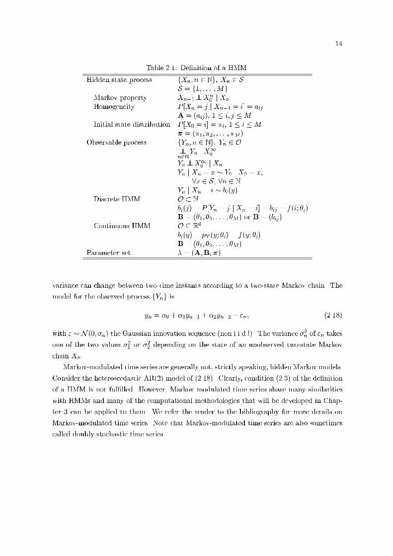
14
Table 2.1: De�nition of a HMM.
Hidden state process fXn; n 2 Ng, Xn 2 SS = f1; : : : ;Mg
Markov property Xn+1??Xn0 j Xn
Homogeneity P [Xn = j j Xn�1 = i] = aijA = (aij), 1 � i; j �M
Initial state distribution P [X0 = i] = �i, 1 � i �M� = (�1; �2; : : : ; �M )
Observable process fYn; n 2 Ng, Yn 2 O??n2N
Yn j X10
Yn??X10 j Xn
Yn j Xn = x � Y0 j X0 = x,
8x 2 S, 8n 2 NYn j Xn = i � bi(y)
Discrete HMM O � N
bi(j) = P [Yn = j j Xn = i] = bij = f(i; �i)
B = (�1; �2; : : : ; �M ) or B = (bij)
Continuous HMM O � Rd
bi(y) = pY (y; �i) = f(y; �i)
B = (�1; �2; : : : ; �M )
Parameter set � = (A;B;�)
variance can change between two time instants according to a two-state Markov chain. The
model for the observed process fYng is
yn = �0 + �1yn�1 + �2yn�2 + "n; (2.18)
with " � N (0; �n) the Gaussian innovation sequence (non i.i.d.!). The variance �2n of "n takes
one of the two values �21 or �22 depending on the state of an unobserved two-state Markov
chain Xn.
Markov-modulated time series are generally not, strictly speaking, hidden Markov models.
Consider the heteroscedastic AR(2) model of (2.18). Clearly, condition (2.3) of the de�nition
of a HMM is not ful�lled. However, Markov modulated time series share many similarities
with HMMs and many of the computational methodologies that will be developed in Chap-
ter 3 can be applied to them. We refer the reader to the bibliography for more details on
Markov-modulated time series. Note that Markov-modulated time series are also sometimes
called doubly stochastic time series.

15
0 100 200 300 400 500 600 700 800 900 1000
3000
2000
1000
0
n
AR(2) process with Markovian heteroscedasticity
Figure 2.2: A Gaussian AR(2) process with Markov-modulated innovation variance.
2.2 Variants and Terminology
2.2.1 Types of HMMs
Hidden Markov models are classi�ed according to the properties of their hidden Markov
chain. There are two particular types of hidden Markov model which are of practical interest:
ergodic hidden Markov models and left-right hidden Markov models. In engineering parlance,
ergodic HMMs are used to model stationary1 systems, while left-right models are used to
model transient behaviors.
2.2.1.1 Ergodic HMMs
An HMM is called ergodic if its hidden Markov process fXng is ergodic. Recall that
necessary and su�cient conditions for a �nite discrete Markov chain such as fXng to be
ergodic are that it must be positive recurrent, aperiodic and irreducible (Resnick 1992).
If all the transitions probabilities are strictly positive, i.e., aij > 0, 8i; j 2 S, the Markov
chain fXng is said to be fully connected. In the engineering literature, fully-connected modelsare often called ergodic models. This can be misleading, since, if full-connectedness is a
su�cient condition for ergodicity, it is not a necessary one.
1Stationary is used here in a loose sense.

16
1 2
34
-a12
�a21
-a11 -
a22
�a34
-a43
-a44
-a33
6a41 ?a14 ?a236a32Ia31
Ra13
a24
�a42
Figure 2.3: A four-state ergodic fully connected model.
Figure 2.3 represents a four-state fully-connected ergodic Markov chain. The correspond-
ing transition matrix would be
A =
0BBBBB@
a11 a12 a13 a14
a21 a22 a23 a24
a31 a32 a33 a34
a41 a42 a43 a44
1CCCCCA
Remark 2.2 Ergodicity of the hidden Markov chain does not necessarily imply ergodicity of
the observed process fYng; an additional stationarity condition is required (see Theorem 2.3).
2.2.1.2 Stationary HMMs
It is often assumed that the initial state distribution � of an ergodic HMM is the unique
stationary distribution ��, solution of
�� = ��A: (2.19)
This assumption makes sense in practice since the state distribution of an ergodic Markov
chain always converges toward the stationary distribution. Note that in this case � =
(A;B;��) is redundant since �� can be computed from A by solving (2.19). For stationary
ergodic HMMs, the parameter set can thus be reduced to � = (A;B).
For non-ergodic HMMs, the solution of (2.19) need not be unique. In any case, if �
is a stationary distribution, the Markov chain fXng is stationary and the HMM is called
stationary. This appellation is justi�ed by the following theorem and its corollary.
17
Theorem 2.2 Let fZn = (Xn; Yn)g de�ne a hidden Markov model. If the hidden Markov
chain fXng is stationary, the complete process fZng is stationary.
Proof. We need to show
P [Zk+nk 2 E] = P [Zn0 2 E]; 8k; n 2 N; 8E = (EX ; EY ) 2 (S �O)n+1:
We have
P [Zk+nk 2 E] = P [Y k+nk 2 EY j Xk+n
k 2 EX ]P [Xk+nk 2 EX ] (2.20)
= P [Y n0 2 EY j Xn
0 2 EX ]P [Xn0 2 EX ] (2.21)
= P [Zn0 2 E]; (2.22)
where the homogeniety properties of Yn j Xn = x have been used. �
Corollary 2.1 If the hidden Markov chain fXng is stationary, the observed process fYngis stationary.
Moreover, if, in addition to being stationary, the hidden Markov chain is irreducible (and
hence ergodic), the observed process fYng is also ergodic.
Theorem 2.3 (Leroux) If fXng is stationary and ergodic, then fYng is ergodic.
Proof. The proof can be found in (Leroux 1992b). �
2.2.1.3 Left-Right HMMs
Left-right HMMs, or Bakis models, are HMMs for which the transition matrixA is upper-
triangular, i.e.,
A =
0BBBBBB@
a11 a12 � � � a1M
0 a22 � � � a2M...
.... . .
...
0 0 � � � aMM
1CCCCCCA
and the initial distribution is the unit vector � = (1; 0; : : : ; 0)0, i.e., the initial state is 1 with
probability one. The state M is necessarily absorbing and is called the �nal state. PIf M
is the only absorbing state, which is generally the case, the Markov chain evolves along the
states in increasing order (any state that is left cannot be revisited later). It follows from the
properties of absorbing Markov chains that the last state (M) will be reached in �nite time
with probability one.
Left-right HMMs are particularly well suited to model stochastic transient processes which
have a particular \temporal signature." For example, left-right HMMs are commonly used

18
1 2 3 4
-a12 -
a23 -a34
-a13
-a24
-a11 -
a22 -a33 -
a44
Figure 2.4: A four-state left-right model.
61
2
3 5
4
-a24
-a35
Ra25
�
a34�
a12
Ra13
Ra46
�a56
-a11 -
a66
-a22 -
a44
-a33
-a55
Figure 2.5: A six-state parallel path left-right model.
in speech processing to model words. The sequence of states (which often corresponds to
phonemes or acoustical units) in a word have a typical time-ordering even if some random
variations are possible. Left-right HMMs can encompass this time-ordering and its variations.
Figures 2.4 and 2.5 represent a four-state left-right Markov model and a six-state left-
right Markov model with two \parallel" paths (only the edges corresponding to non-zero
transition probabilities are drawn). In the �rst case, the transition matrix would have the
upper-triangular banded structure:
A =
0BBBBB@
a11 a12 a13 0
0 a22 a23 a24
0 0 a33 a34
0 0 0 a44
1CCCCCA :
2.2.2 Variable Duration HMMs
Variable duration HMMs (Rabiner 1989, Levinson 1986) are obtained by replacing the
hidden Markov process fXng by a discrete-time semi-Markov process. That is, once Xn

19
i j k
-aij
�aji
-ajk
�akj
-di(`) -
dj(`) -dk(`)
i kj3 j2 j1
-di(`)
-dj(3)aij
- dj(2)aij
-dj(1)aij
�ajk
-1 -1 -ajk
-dk(`)
�dj(1)akj
�dj(2)akj�dj(3)akj
Figure 2.6: Equivalence between a semi-Markov chain and a Markov chain.
enters state i, it stays in i for a random amount of time ` governed by a distribution di(`),
k 2 N0 , then jumps to a di�erent state j with probability aij . While Xn is in state i, the
r.v.s Yn are observed independently with class-conditional distribution bi(y). That is, ` i.i.d.
observations of Yn are made while Xn = i. A variable duration HMM is de�ned by the
same set of parameters as a standard HMM plus a set of \state duration" distributions di(`),
k 2 N0 , i = 1; 2; : : : ;M .
If the time that the semi-Markov process can spend in a single state is bounded, i.e., if
di(`) = 0 for t > Ki, the variable duration HMM de�ned on the semi-Markov process can be
replaced by a standard HMM with shared state-conditional distributions. This is illustrated
in Figure 2.6, where Kj = 3 and the states j1, j2, and j3 share the same class-conditional
distribution: bj1(y) = bj2(y) = bj3(y) = bj(y). For clarity, only the transitions connecting j
to i and k have been represented, and only the state j has been expanded. Because of this
equivalence, most of the results presented in this work for standard HMMs will also apply to
variable duration HMMs.
Variable duration HMMs with semi-Markov state chains are sometimes desirable to model
physical signals for which the exponential law associated with the state duration distribution
of the Markov chain does not provide a realistic model (Burshtein 1995). In addition to
the variable duration HMMs based on discrete semi-Markov processes presented here, mod-
els based on continuous semi-Markov processes with discrete state spaces (Levinson 1986,
Burshtein 1995) and models based on non-homogeneous Markov chains with discrete state
spaces (Sin & Kim 1995) have also been proposed.
2.2.3 Exogenous Inputs HMMs
A hidden Markov model can be viewed as a system whose internal state Xn evolves in
a Markovian fashion according to the state transition probabilities A, and whose output,
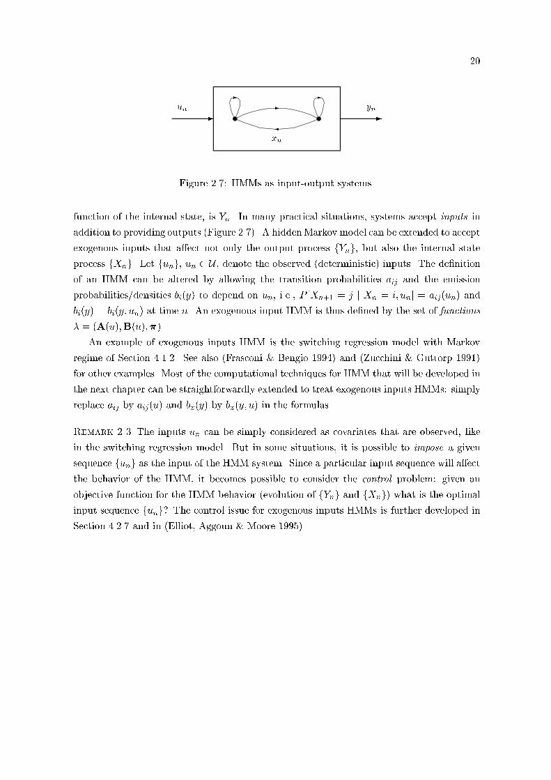
20
-
�
- -
- -
xn
un yn
Figure 2.7: HMMs as input-output systems.
function of the internal state, is Yn. In many practical situations, systems accept inputs in
addition to providing outputs (Figure 2.7). A hiddenMarkov model can be extended to accept
exogenous inputs that a�ect not only the output process fYng, but also the internal state
process fXng. Let fung, un 2 U , denote the observed (deterministic) inputs. The de�nition
of an HMM can be altered by allowing the transition probabilities aij and the emission
probabilities/densities bi(y) to depend on un, i.e., P [Xn+1 = j j Xn = i; un] = aij(un) and
bi(y) = bi(y; un) at time n. An exogenous input HMM is thus de�ned by the set of functions
� = (A(u);B(u);�).
An example of exogenous inputs HMM is the switching regression model with Markov
regime of Section 4.1.2. See also (Frasconi & Bengio 1994) and (Zucchini & Guttorp 1991)
for other examples. Most of the computational techniques for HMM that will be developed in
the next chapter can be straightforwardly extended to treat exogenous inputs HMMs: simply
replace aij by aij(u) and bx(y) by bx(y; u) in the formulas.
Remark 2.3 The inputs un can be simply considered as covariates that are observed, like
in the switching regression model. But in some situations, it is possible to impose a given
sequence fung as the input of the HMM system. Since a particular input sequence will a�ect
the behavior of the HMM, it becomes possible to consider the control problem: given an
objective function for the HMM behavior (evolution of fYng and fXng) what is the optimalinput sequence fung? The control issue for exogenous inputs HMMs is further developed in
Section 4.2.7 and in (Elliot, Aggoun & Moore 1995).

21
Chapter 3
Computations with Hidden Markov
Models
In this chapter, algorithms are proposed to solve the three basic computational problems
of hidden Markov modeling. The three basic problems are:
1. Given an observation sequence yN0 and an HMM �, compute the likelihood p(yN0 ;�).
2. Given an observation sequence yN0 and an HMM �, �nd the optimal estimate of the
state Xn for some n 2 f0; 1; : : : ; Ng, or of the state sequence XN0 = (X0;X2; : : : ;XN ).
3. Given a set of K observation sequences fyN0 [k]; k = 1; 2; : : : ;Kg,1 and an HMM struc-
ture, compute an estimate of the HMM parameter �. More precisely, compute the
maximum-likelihood (ML) estimate of �.
We use yN0 = (y0; y1; : : : ; yN�1), yn 2 O, to denote a length N + 1 realization of the
observed process of an HMM. We will also make use of the following notations: a length
N + 1 realization of the state process of an HMM will be denoted by xN0 = (x0; x1; : : : ; xN ),
xn 2 S, and � = (A;B; �) will represent the set of parameters of this HMM. The subsequences
(yk; yk+1; : : : ; y`) and (xk; xk+1; : : : ; x`), 0 � k < ` � N , of yN0 and xN0 will be denoted by y`k
and x`k, respectively. The probability mass function of Y `k = (Yk; Yk+1; : : : ; Y`) for a discrete
HMM and the probability density function of Y `k for a continuous HMM, given an HMM
structure with parameter �, will be similarly denoted by p(y`k;�), for y`k 2 O`�k+1. That is,
p(y`k;�) =
8<: P [Y `
k = y`k;�] for DHMMs
pY `k(y`k;�) for CHMMs
:
Unless it is not clear from the context, p(y`k;�) will be called the likelihood or the distribution
of Y `k given an HMM � without further reference to the discrete or continuous nature of the
1The K observation sequences yN0 [k] are assumed of same lengths for simplicity, but the results that will
be presented in the sequel can be straightforwardly modi�ed to handle sequences of di�erent lengths.

22
model. For compactness, we will also often shorten expressions like P [X`k = x`k j Y N
0 = yN0 ;�]
into P [x`k j yN0 ;�].
3.1 Computation of the Likelihood
By the total probability theorem, we have
p(yN0 ;�) =X
xN0 2ON+1
p(yN0 jxN0 ;�)P [xN0 ;�]; (3.1)
where
p(yN0 jxN0 ;�) = bx0(y0)bx1(y1) � � � bxN (yN ); (3.2)
P [xN0 ;�] = �x0ax0x1ax1x2 � � � axN�1xN ; (3.3)
with the proper interpretation of p(�;�) and bx(�) as probability mass function or probability
density function whether the HMM is discrete or continuous. Combining (3.1), (3.2), and
(3.3), we get
p(yN0 ;�) =X
xN0 2ON+1
�x0bx0(y0)ax0x1bx1(y1) � � � axN�1xN bxN (yN ): (3.4)
The calculation of p(Y N0 j�) according to its direct de�nition (3.4) involves O(NMN )
operations (product and summations), which is computationally infeasible, even for moderate
size HMMs. Clearly, a more e�cient procedure is needed to perform the calculation of
p(yN0 ;�). Such a procedure exists, which computes the likelihood in O(M2N) time (Baum
& Eagon 1967). It is sometimes called the forward-backward (FB) algorithm. In fact, the
forward-backward algorithm consists of two separate algorithms: the forward algorithm and
the backward algorithm.
3.1.1 The Forward Algorithm
The forward algorithm is based on the following recursive relation. Let �n(i), 0 � n � N ,
1 � i �M , be the forward variable de�ned by
�n(i) = p(yn0 ;Xn = i;�): (3.5)

23
Table 3.1: The forward algorithm.
1. Initialization: �0(i) = �ibi(y0), 1 � i �M .
2. Iteration: for n = 0; 1; : : : ; N � 1,
�n+1(j) =
MXi=1
�n(i)aij
!bj(yn+1); 1 � j �M:
3. Termination: p(yN0 ;�) =MXi=1
�N (i).
From the conditional independence properties of HMMs, we have, for 0 � n � N ,
�n+1(j) =MXi=1
p(yn+10 ;Xn+1 = jjXn = i;�)P [Xn = i;�]
=MXi=1
p(yn+10 jXn+1 = j;Xn = i;�)P [Xn = i;�]P [Xn+1 = jjXn = i;�]
=MXi=1
p(yn+1jXn+1 = j;�)p(yn0 ;Xn = i;�)P [Xn+1 = jjXn = i;�]
=
MXi=1
�n(i)aij
!bj(yn+1) (3.6)
and
�0(i) = �ibi(y0): (3.7)
The sequence of operations required for the computation of the forward variable �n(j) is
illustrated on Figure 3.1. By induction, we deduce the forward algorithm for the computation
of p(yN0 ;�) of Table 3.1.
The forward algorithm can be implemented on a lattice structure like that of Figure 3.2.
It is easy to see that the calculation of p(yN0 ;�) with the forward algorithm involves O(M2N)
operations, i.e., the forward algorithm has a linear complexity in N .
Example 3.1 Consider a length 100 sequence obtained from an HMM with a �ve-state
hidden Markov chain, the calculation of its likelihood according to the direct de�nition (3.4)
requires on the order of 100 � 5100, that is, on the order of 1072 operations are required! With
the forward recursion, there are on the order of 52 � 100 = 2500 operations.
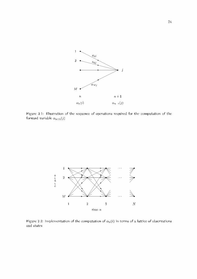
24
n
�n(i)
M
.
.
.
2
1
n+ 1
�n+1(j)
j
ja1j
za2j
-
*aMj
Figure 3.1: Illustration of the sequence of operations required for the computation of the
forward variable �n+1(j).
1
2
.
.
.
.
.
.
.
.
.
M
.
.
.
-
j
^
*
-
R-
�
�
-
j
^
*
-
R-
�
�
: : :
: : :
: : :
s
ta
te
1 2 3 N
time n
Figure 3.2: Implementation of the computation of �n(i) in terms of a lattice of observations
and states.

25
Table 3.2: The backward algorithm.
1. Initialization: �N (i) = 1, 1 � i �M .
2. Iteration: for n = N � 1; N � 2; : : : ; 0,
�n(i) =MXj=1
aijbj(yn+1)�n+1(j); 1 � i � N:
3. Termination: p(yN0 ;�) =MXi=1
�N (i)�i.
3.1.2 The Backward Algorithm
De�ne the backward variable �n(i) as
�n(i) =
8<: p(yNn+1jXn = i;�) for 0 � n � N � 1
1 for n = N: (3.8)
Like the forward variable �n(i), the backward variable �n(i) can be computed recursively.
The backward recursion is de�ned by
�n(i) =MXj=1
p(yNn+2; yn+1;Xn+1 = jjXn = i;�)
=MXj=1
p(yNn+2jXn+1 = j;Xn = i;�)p(yn+1jXn+1 = j;Xn = i;�)P [Xn+1 = jjXn = i;�]
=MXj=1
aijbj(yn+1)�n+1(j) (3.9)
for 0 � n � N � 1. The backward algorithm of Table 3.2 follows by induction. Like
the forward algorithm, the backward algorithm can be implemented on a lattice structure
(Figure 3.3). Its complexity is also O(M2N).
Combining the forward and backward algorithm, it is possible to write the likelihood as
p(yN0 ;�) =MXi=1
MXj=1
�n(i)aijbj(yn+1)�n+1(j) (3.10)
for 0 � n � N � 1.
3.1.3 Matrix Formulation
Several of the formulae derived in this section are much more compact in matrix notation.
Let 1 be theM�1 column vector (1; 1; : : : ; 1)0 and letBn = diag (b1(yn); b2(yn); : : : ; bM (yn)).

26
i
n
�n(i)
n+ 1
�n+1(j)
M
.
.
.
2
1
�ai1
9ai2
�
YaiM
Figure 3.3: Illustration of the sequence of operations required for the computation of the
backward variable �n(i).
Also, let �n = (�n(1); �n(2); : : : ; �n(M))0 and �n = (�n(1); �n(2); : : : ; �n(M))0. Then, the
forward recursion can be written
�n+1 = Bn+1A0�n; n = 0; 1; : : : ; N � 1: (3.11)
The backward recursion can be written
�n = ABn+1�n+1; n = N � 1; : : : ; 1; 0: (3.12)
The initial values for (3.11) and (3.12) are �0 = B0� and �N = 1, respectively. The
likelihood of yN0 is given by
p(yN0 ;�) = �0n�n (3.13)
for any n in f0; 1; : : : ; Ng. Expanding the recursion for �n and �n, we get
p(yN0 ;�) = �0B0AB1A � � �BN�1ABN1: (3.14)
3.2 Computation of the Most Likely Sequence of States
Let n(i) be the a posteriori probability of state i given a realization yN0 ,
n(i) = P [Xn = ijyN0 ;�]; 1 � i �M; 0 � n � N: (3.15)
By Bayes's rule, we have
n(i) =p(yn0 ; y
Nn+1jXn = i;�)P [Xn = i;�]
p(yn0 ; yNn+1;�)
=p(yn0 ;Xn = i;�)p(yNn+1jXn = i;�)MXi=1
p(yn0 ;Xn = i;�)p(yNn+1jXn = i;�)
;

27
n� 1
.
.
.
n
�n(i)
i
jz-
*aijbj(yn+1)
� -
j
n+ 1
�n+1(j)
n+ 2
.
.
.
�9�
Y
Figure 3.4: Illustration of the sequence of events required for the computation of the joint
event that the hidden Markov chain is in state i at time n and in state j at time n+ 1.
that is,
n(i) =�n(i)�n(i)MXi=1
�n(i)�n(i)
: (3.16)
Equation (3.16) implies that n(i) can be computed in linear time by the forward-backward
algorithm. For later use, de�ne similarly �n(i; j) = P [Xn = i;Xn+1 = jjyN0 ;�] to be the a
posteriori transition probability from state i to state j at time n. We have,
�n(i; j) =�n(i)aijbj(yn+1)�n+1(j)
MXi=1
MXj=1
�n(i)aijbj(yn+1)�n+1(j)
; (3.17)
which can again be computed in linear time by the forward-backward algorithm (Figure 3.4).
Note thatPMj=1 �n(i; j) = n(i).
The estimate of state Xn, 0 � n � N given yN0 that minimizes the probability of error,
or, equivalently, that maximizes the expected number of correct decisions, is the maximum
a posteriori probability estimate
~xn = argmaxx2S
n(x)
= argmaxx2S
�n(x)�n(x): (3.18)
For the complete state sequence XN0 , a possible estimate is ~xN0 = (~x0; ~x1; : : : ; ~xN ). while it
maximizes the expected number of correct state decisions. This estimate su�ers from the
fact that there is no guarantee that P [XN0 = ~xN0 ;�] > 0 if the Markov chain is not fully
connected. It seems realistic to expect from the estimate of XN0 that it belongs to the set of
sequences with non-null probability. One such estimate is the most likely sequence of states

28
Table 3.3: The Viterbi algorithm.
1. Initialization: �0(i) = �ibi(y0), 1 � i �M .
2. Iteration: for n = 0; 2; : : : ; N � 1,
�n+1(j) = bj(yn+1) max1�i�M
[�n(i)aij ] ; 0 � j �M;
n+1(j) = arg max1�i�M
[�n(i)aij ] ; 0 � j �M:
3. Termination:
P = max1�i�M
�N (i);
xN = arg max1�i�M
�N (i):
4. Backtracking: for n = N � 1; N � 2; : : : ; 0,
xn = n+1(xn+1):
(MLSS) given by
xN0 = arg maxxN0 2S
N+1P [xN0 jyN0 ;�];
= arg maxxN0 2S
N+1P [xN0 ; y
N0 ;�]: (3.19)
The maximization (3.19) can be performed e�ciently via a dynamic programming algo-
rithm known as the Viterbi decoder or Viterbi algorithm (Forney 1973) which is similar to
the forward-backward algorithm. Let �n(i) be the real valued function de�ned by
�n(i) =
8<: maxxn�10
p(xn�10 ;Xn = i; yn0 ;�) for 1 � n � Np(y0;X0 = i;�) for n = 0
; (3.20)
and let n(x) be the S-valued function de�ned by
n(j) = arg max1�i�M
[�n�1(i)aij ] ; 1 � n � N: (3.21)
A little thought should convince the reader that the dynamic programming algorithm of
Table 3.3 does provide the desired maximizer of (3.19). The number of operations required
for the computation of the most likely sequence of states by the Viterbi algorithm is O(M2N).

29
3.3 Computation of the Maximum Likelihood Estimate of the
Model Parameters
One of the most commonly used estimation methods for HMMs is the maximum likeli-
hood (ML) method. The ML method has mostly been used for HMMs because an e�cient
algorithm for its implementation is available. This algorithm, which is an instance of the
more general Expectation-Maximization (EM) algorithm (Dempster, Laird & Rubin 1977)
for likelihood maximization, was originally introduced by Baum & Eagon (1967), and is often
called the Baum-Welsh algorithm in the HMM literature. In addition, the ML estimator of
HMM parameters possesses good statistical properties, such as consistency (see Chapter 5).
3.3.1 Maximum Likelihood Estimator
Assume that the structure of the HMM is known, that is, the type and dimension of
the hidden Markov chain are �xed and the (parametric) form of the distributions bi(y) is
given. The HMM is thus a parametric model completely de�ned by � = (A;B;�). Let
� = A � B � P be the set of admissible values for �, where A, B, and P are the sets of
admissible values for A, B, and �, respectively. For example, for a fully-connected HMM,
A is the set of M �M strictly positive stochastic matrices. Given a realization of Y N0 , the
maximum-likelihood estimate of � is2
� = argmax�2�
p(yN0 ;�)
= argmax�2�
L(�) (3.22)
with L(�) = ln p(yN0 ;�) the log-likelihood function. For all but the most trivial HMMs,
there is no known way to solve analytically (3.22). It is necessary to resort to iterative
numerical optimization methods. The most popular numerical maximization method is the
Baum-Welsh algorithm.
3.3.2 The Baum-Welsh Algorithm
The estimation of the parameters of a hidden Markov model can easily be casted as a
missing data problem. For an HMM, the observed (incomplete) data is Y N0 and the complete
data is ZN0 = (Z0; Z1; : : : ; Zn), with Zn = (Xn; Yn). The likelihood can thus be maximized
by the EM algorithm.3
Let Q(��; �) be the auxiliary function
Q(��; �) = E�[ln p(ZN0 ; ��) j yN0 ]; (3.23)
2This de�nition assumes that the minimizer is unique. This is usually not the case, see Section 5.2.1 for
details3The reader unfamiliar with the EM algorithm can �nd its de�nition and a review of its basic properties
in Appendix B.

30
where
p(zN0 ;��) = ��x0
�bx0(y0)�ax0x1�bx1(y1) � � � �axN�1xN
�bxN (yN )
denotes the distribution of the complete data for an HMM ��. Given a current approximation
� of �, the next approximation �� of � is obtained by the EM iteration de�ned by (Dempster
et al. 1977)
1. E-step: Determine Q(��; �).
2. M-step: Choose �� 2 argmax��2�
Q(��; �).
But we have
Q(��; �) =X
xN0 2SN+1
"ln ��x0 +
N�1Xn=0
ln �axnxn+1 +NXn=0
ln�bxn(yn)
#P [xN0 j yN0 ;�]
=Xx02S
ln ��x0P [x0 j yN0 ;�] +N�1Xn=0
Xxn+1n 2S2
ln �axnxn+1P [xn+1n j yN0 ;�]
+NXn=0
Xxn2S
ln bxn(yn)P [xn j yN0 ;�]
=MXi=1
0(i) ln ��i +MXi=1
MXj=1
N�1Xn=0
�n(i; j) ln �aij +MXi=1
NXn=0
n(i) ln�bi(yn): (3.24)
with n(i) and �n(i; j) de�ned by (3.16) and (3.17). Hence, the M-step decomposes into
three separate maximization problems, and the EM algorithm reduces to the set of three
re-estimation formulae:
�� 2 argmax��2P
MXi=1
0(i) ln ��i; (3.25)
�A 2 argmax�A2A
MXi;j=1
N�1Xn=0
�n(i; j) ln �aij; (3.26)
�B 2 argmax�B2B
MXi=1
NXn=0
n(i) ln�bi(yn): (3.27)
Going any further requires making assumptions on A, B, P, and bi(y).Consider �rst the maximization (3.25) and (3.26). The most general sets of admissible
values for � and A are simply
P =
(� : � 2 RM ;
MXi=1
�i = 1
);
i.e., � must be a stochastic vector, and
A =
8<:A = (aij) : A 2 RM�M ;
MXj=1
aij = 1
9=; ;

31
i.e., A must be a row stochastic matrix. With these linear constraints on the parameters,
the extrema can be found by Lagrange's multipliers method. For example, the maximization
(3.25) leads to the system of M + 1 equations8>>>>>><>>>>>>:
0(1)1�1
+ � = 0...
0(M) 1�M
+ � = 0
�1 + �2 + � � �+ �M � 1 = 0
where � denotes Lagrange's multiplier. Solving for �i yields the unique maximizer
��i = 0(i): (3.28)
Similarly, for (3.26) we get
�aij =
N�1Xn=0
�n(i; j)
N�1Xn=0
MXj=1
�n(i; j)
=
N�1Xn=
�n(i; j)
N�1Xn=0
n(i)
: (3.29)
An intuitively satisfying interpretation of these re-estimation formulae can be obtained by
observing that (3.28) and (3.28) can also be written as
��i = Eh1fX0=ig j Y N
0 = yN0
i; (3.30)
and
�aij =
E
"N�1Xn=0
1fXn=ig1fXn+1=jg
���Y N0 = yN0
#
E
"N�1Xn=0
1fXn=ig
���Y N0 = yN0
# ; (3.31)
where 1E denotes the indicator function of the event E.
That is, ��i is the expected number of times the hidden chain is in state i at time n = 0
and �aij is the ratio of the expected number of times the hidden chain e�ects a transition from
state i to state j to the expected number of times the hidden chains starts a transition from
state i, all expectations being taken conditional to yN0 . Recall that, for a directly observed
discrete Markov chain fXng, the maximum likelihood estimate of the transition probability
aij is given by (Resnick 1992)
aij =
N�1Xn=0
1fXn=ig1fXn�1=jg
N�1Xn=0
1fXn=ig
: (3.32)

32
Table 3.4: The Baum-Welsh algorithm.
1. Find an initial estimate �(0) of �.
2. Set � = �(0).
3. Compute �� by the re-estimation formulae:
��i = 0(i) 1 � i �M:
�aij =
N�1Xn=0
�n(i; j)
N�1Xn=0
n(i)
1 � i; j �M;
��i 2 argmax��2�
NXn=0
n(i) ln f(yn; ��); 1 � i �M;
where n(i) and �n(i; j) are computed with respect to �.
4. Set � = ��.
5. Go to 3 unless some ad hoc convergence criterion is met.
6. Set � = ��.
Thus, the re-estimation formula (3.31) can be viewed as the maximum likelihood estimate
(3.32) for the hidden Markov chain, in which the state indicator statistics have been replaced
by their \best estimates," i.e., their conditional estimates given the observed data yN0 .
Suppose now that the distribution bi(y) can be written as
bi(y) = f(y; �i); �i 2 �;
for some parametric function f(� ; �) and some parameter set �. We have B = (�1; �2; : : : ; �N )
and B = �M . Then, (3.27) decomposes into M separate maximization problems:
��i 2 argmax��2�
NXn=0
n(i) ln f(yn; ��); 1 � i �M: (3.33)
Gathering (3.28), (3.29), and (3.33), we obtain the Baum-Welsh algorithm of Table 3.4. The
initial estimate �(0) is either chosen arbitrarily, or obtained by another estimation method
(e.g., the k-means clustering method of Section 5.2.5). Solution of (3.33) requires the pos-
tulation of a particular form for f(y; �). In many cases, an analytical expression for the
maximizers ��i will exist. Some examples are developed in the next section.
33
Remark 3.1 The assumptions made on the sets of admissible values A and P for the deriva-
tion of the Baum-Welsh algorithm are less restrictive than they might seem. Consider equa-
tions (3.29) and (3.17), clearly, any aij that is set to zero initially will remain at zero through-
out the estimation procedure. Hence, the initial values of the aij in the Baum-Welsh algorithm
provide an e�cient way to include structural constraints on the stochastic matrix A. For
example, a left-right structure can be imposed on the HMM by using an upper triangular
initial estimate A(0). Similarly, any �i that is set to zero initially will remain at zero.
Remark 3.2 The Baum-Welsh re-estimation formulae predate the EM algorithm by ten
years. They were originally obtained by Baum and his co-workers (Baum & Eagon 1967,
Baum, Petrie, Soules & Weiss 1970) using a di�erent approach than the EM argument pre-
sented here. They can also be obtained as an iterative solution to a constrained maximization
problem which can be solved by the classical method of Lagrange multipliers (Levinson, Ra-
biner & Sondhi 1983).
3.3.3 Examples
There exists an analytical solution to (3.33) for some form of parametric distributions
(probability mass functions or probability density functions) bi(y) = f(y; �i). Combining
this solution with (3.28) and (3.29) provides the complete set of re-estimation formulae for
the Baum-Welsh algorithm in closed form. The solution to (3.33) for the �ve examples of
HMMs introduced in Chapter 2 (non-parametric DHMM, binomial DHMM, Poisson DHMM,
Gaussian CHMM, Mixture of Gaussians CHMM) are now given.
3.3.3.1 Non-Parametric Discrete HMM
For a non-parametric discrete hidden Markov model, we have
bi(j) = P [Yn = j j Xn = i] = bij = f(j; �i); j 2 O = f1; 2; : : : ; Lg;
with �i the row vector (bi1; bi2; : : : ; biM ). The set of admissible values � � [0; 1]L corresponds
to the stochastic constraintPLj=1 bij = 1. Observe that
NXn=0
n(i) ln bi(yn) =LXj=1
X0�n�Nyn=j
n(i) ln bi(j):
By analogy with (3.28) and (3.29), we can write directly the solution to (3.33) as
�bij =
X0�n�Nyn=j
n(i)
NXn=0
n(i)
; 1 � i �M; 1 � j � L: (3.34)

34
Equation (3.34) can be interpreted as the ratio of the expected number of times the hidden
chain is in state i and the observed symbol is j, given yN0 , to the expected number of time
the hidden chain is in state i. To see this, rewrite (3.34) as
�bij =
E
"NXn=0
1fYn=jg j Y N0 = yN0
#
E
"NXn=0
1fXn=ig j Y N0 = yN0
# :
3.3.3.2 Binomial Discrete HMM
For a binomial discrete hidden Markov model, we have
bi(y) =
L
y
!�yi (1� �i)L�y; 0 � y � L; (3.35)
and � = [0; 1]. It is not di�cult to show that the solution to (3.33) is
��i =
1
L
NXn=0
n(i)yn
NXn=0
n(i)
: (3.36)
3.3.3.3 Poisson Discrete HMM
For a Poisson discrete hidden Markov model, we have
bi(y) =e��i�
yi
y!; y 2 N; (3.37)
and � = R+ . The maximizer of (3.33) can be obtained by
��i =
NXn=0
n(i)yn
NXn=0
n(i)
: (3.38)
3.3.3.4 Gaussian Continuous HMM
For a continuous HMM with d-dimensional Gaussian conditional distributions, we have
bi(y) =1
(2�)d=2j�ij1=2exp
��12(y � �i)0��1
i (y � �i)�= f(y; �i); y 2 Rd ;
(3.39)

35
with �i = f�i;�ig and � = Rd �Rdd, where Rdd denotes the set of d � d positive de�nite
symmetric matrices. It is not di�cult to show that the re-estimation formula (3.33) becomes
��i =
NXn=1
n(i)yn
NXn=1
n(i)
(3.40)
��i =
NXn=1
n(i)(yn � ��i)(yn � ��i)0
NXn=1
n(i)
(3.41)
for i = 1; 2; : : : ;M . Positive de�niteness of ��i is guaranteed with probability one if N > d
(Liporace 1982). In both formulae, the new estimates can be regarded as weighted sam-
ple means and weighted sample covariance matrices with the weights proportional to the a
posteriori state probabilities given the current value of �.
3.3.3.5 Mixture of Gaussians Continuous HMM
In the mixture of Gaussians case, we have
bi(y) = f(y; �i) =KiXk=1
�i;kgi;k(y); y 2 Rd ; (3.42)
with
gi;k(y) =1
(2�)d=2j�i;kj1=2exp
��12(y � �i;k)0��1
i;k (y � �i;k)�
(3.43)
and �i = (�i;�i;�i). Using the analogy between a mixture of Gaussians HMM and an
\expanded" Gaussian HMM (Figure 2.1), it is easy to show that the maximizer of (3.33) is
given by
��i;k =
NXn=0
n(i)�n(i; k)
NXn=0
n(i)
(3.44)
��i;k =
NXn=0
n(i)�n(i; k)yn
NXn=0
n(i)�n(i; k)
(3.45)
��i;k =
NXn=0
n(i)�n(i; k)(yn � ��i;k)(yn � ��i;k)0
NXn=0
n(i)�n(i; k)
(3.46)

36
with
�n(i; k) =�i;kgi;k(yn)
bi(y):
for i = 1; 2; : : : ;M , k = 1; 2; : : : ;Ki. Alternately to (3.46), a heuristic re-estimation equation
for the covariance matrices can be written as (Juang & Rabiner 1985a)
��i;k =
NXn=0
n(i)�n(i; k)(yn � �i;k)(yn � �i;k)0
NXn=0
n(i)�n(i; k)
(3.47)
It is obvious that the iterative re-estimation scheme obtained by using (3.47) instead of
(3.46) admits the same sets of �xed points. In practice, it has been found that both re-
estimation algorithms provide similar results (Huang, Ariki & Jack 1990). This is because
�i is approximately equal to ��i in contiguous iterations.
3.3.4 Convergence Properties of the Baum-Welsh Algorithm
Consider the sequence of iterates f�(0); �(1); �(2); : : : g obtained by the Baum-Welsh algo-
rithm and the associated sequence of likelihoods fL(�(0)); L(�(1)); L(�(2); : : : g. What can be
said of the convergence of these sequences toward the maximizer � and the maximum and
L(�)?
Since the Baum-Welsh algorithm is an instance of the EM algorithm for likelihood maxi-
mization, it inherits of the general convergence properties of the EM algorithm (see (Dempster
et al. 1977, Wu 1983) and Appendix B). In the most general case, it can be shown that the
sequence L(�(p)) increases monotonously, i.e., L(�(p+1)) � L(�(p)) (Theorem B.1). In order
to obtain stronger results on the convergence of �(p) and L(�(p)), it is necessary to make
additional assumptions on the class-conditional distributions bi(y) and on the parameter set
�. These stronger results can be obtained either via the EM convergence theorems of Wu
(1983) or directly via an algebraic approach. Many of the convergence properties of the EM
algorithm were originally proven for the particular case of HMM by Baum and his co-workers
using a di�erent approach than that of Wu (1983).
For example, for non-parametric discrete HMMs, the Baum-Eagon inequality for growth
functions on manifolds (1967) can be applied to show that any �xed point of the re-estimation
formulae is necessarily a critical point of L(�).
Theorem 3.1 (Baum & Eagon) Let p(x) = p(fxijg) be a polynomial with nonnegative
coe�cients homogeneous of degree d in its variables xij. Let x = fxijg be any point of the
manifold
� =
8<:fxijg : xij � 0;
qiXj=1
xij = 1; i = 1; : : : ; p; j = 1; : : : ; qi
9=; :

37
If T : �! � is the transformation de�ned by
T (x)ij =
xij@P
@xij
�����x
qiXj=1
xij@P
@xij
�����x
; (3.48)
then p(T (x)) > p(x) unless T (x) = x.
Proof. The proof can be found in (Baum & Eagon 1967). �
Corollary 3.1 Any �xed point of x(p+1) = T (x(p)) is also a critical point of p(x).
Other corollaries and extensions of the Baum-Eagon inequality can be found in (Baum &
Eagon 1967, Baum & Sell 1968, Baum et al. 1970, Baum 1972, Gopalakrishnan, Kanevsky,
N�adas & Nahamoo 1991).
Clearly, for a non-parametric discrete HMM like that of Section 2.1.1, the likelihood L(�)
is a polynomial in aij , bij, and �i with domain �, where � is the Cartesian product of the
sets of admissible values for the stochastic matrices and vector A, B, and �. Therefore, the
Baum-Eagon inequality can be applied. It is not di�cult to show (Levinson et al. 1983) that
the re-estimation formulae (3.28), (3.29), and (3.34) are equivalent to
��i =
�i@L(�)
@�iMXk=1
�k@L(�)
@�k
������������
; (3.49)
�aij =
aij@L(�)
@aijMXk=1
aik@L(�)
@aik
������������
; (3.50)
�bij =
bij@L(�)
@bijMXk=1
bik@L(�)
@bik
������������
: (3.51)
Hence, it follows from the corollary of the Baum-Eagon inequality that any �xed point of
the re-estimation formulae is a stationary point of the likelihood L(�). From the general
properties of iterative procedures, it can be concluded that the sequence f�(0); �(1); �(2); : : : gwill converge toward a local maxima of L(�) for almost all starting point.
A similar result can be obtained for continuous HMMs when bi(y) belongs to a certain
class of elliptically symmetrical pdfs (Liporace 1982) or mixtures thereof (Juang, Levinson &
Sondhi 1986).

38
Remark 3.3 The algorithmic convergence of �(k) toward �, which is a deterministic property
of the algorithm for a given sample yN0 , should not be confused with the stochastic convergence
of the maximum likelihood estimate � toward the true value of � when the sample length N
tends to in�nity (consistency of the ML estimator). The stochastic convergence properties of
the ML estimator are the subject of Section 5.2.4.
3.3.5 Direct Maximization of the Likelihood
Instead of the Baum-Welsh re-estimation algorithm, it is also possible to use standard
constrained optimization techniques to �nd the maximizer of (3.22), e.g., gradient-based
optimization methods (Levinson et al. 1983, MacDonald & Raubenheimer 1995, Huo & Chan
1993). The gradient of the likelihood rL(�) can be computed by a variant of the forward-
backward algorithm. For example, the derivative of p(yN0 ;�) with respect to aij is obtained
by applying the formula for di�erentiating a product to (3.10), yielding
@p(yN0 ;�)
@aij=
N�1Xn=0
�n(i)bj(yn+1)�n+1(j):
3.3.6 Multiple Observation Sequences
If, instead of a single observation sequence yN0 , we are given a set of K observation
sequences
Y = fyN0 [k]; k = 1; 2; : : : ;Kg;
where yN0 [k] = (y0[k]; y1[k]; : : : ; yN [k]), the re-estimation procedure can be straightforwardly
modi�ed to maximize L(�) = ln p(Y;�) over �. Assuming that every observation sequence is
independent of every other observation sequence, we have
L(�) =KXk=1
ln p(fyN0 [k];�):
Following the same approach as in the single sequence case, we get the re-estimation formula
for aij
�aij =
KXk=1
Nk�1Xn=0
�kn(i; j)
KXk=1
Nk�1Xn=0
kn(i)
1 � i; j �M; (3.52)
where �kn(i; j) and kn(i) can be computed by a forward-backward procedure based on forward
variables �kn(i) and backward variables �kn(i) calculated for y
N0 [k]. Similarly, (3.28) and (3.33)

39
become
��i =KXk=1
kn(i) (3.53)
��i 2 argmax��2�
KXk=1
NKXn=0
kn(i) ln f(yn[k];��) (3.54)
The modi�cations of the speci�c re-estimation formulae of Section 3.3.3 follows directly.
The re-estimation formulae for multiple observation sequences are particularly interesting
for non-ergodic HMMs, e.g., for left-right HMMs. It is obvious that it is not possible to obtain
consistent estimates for all the parameters of a left-right HMM from a single, long, observation
sequence yN0 since, as soon as the hidden Markov chain has reached the �nal absorbing state,
the observed part of the HMM Yn becomes i.i.d., and the rest of the sequence provide no
further information about earlier states. Hence, one has to use multiple observation sequences
in order to make reliable estimates of the model parameters associated with transient states.
Note that N has to be large enough so that the complete left-right chain of states can be
visited. In that respect, note also that the assumption that all the samples have an equal
length N is not crucial since it is always possible to complete a shorter sample sequence
yNk0 [k], Nk < N , with N �Nk \dummy" observations associated with the terminal state of
the left-right HMM that do not a�ect the likelihood. The re-estimation formulae presented
above can be straightforwardly modi�ed to handle this case by replacing the summation on
n from 1 to N by a summation on n from 1 to Nk.
3.4 Practical Implementation Issues
There are many practical issues arising during the implementation on a computer of the
forward-backward, Viterbi, and Baum-Welsh algorithms for hidden Markov modeling. The
most important will now be highlighted. Many solutions to these implementation problems
can be found in the speech recognition literature, for example, in (Rabiner 1989) or in (Huang
et al. 1990).
3.4.1 Thresholding
The amount of computation in the forward-backward algorithm can be reduced by thresh-
olding the forward and backward variables. If, during the course of the forward computation,
certain �n(i) become very small relative to other �n(i) at time n, it has been observed in
practice that these small �n(i) can be set to zero without signi�cantly a�ecting the perfor-
mance. Since the components set to zero do not intervene in the summation (3.6), this can
reduce the computational load signi�cantly for large M . Usually, the �n(i) are set to zero
according to a \thresholding" logic (Huang et al. 1990): at time n, any �n(i) that is less than
Cmaxi �n(i) for some empirical constant 0 < C < 1 is set to zero.

40
Pursuing this \thresholding" idea further and keeping only one state in the summation
at time n will yield the Viterbi approximation of the likelihood of Section 5.2.5 and the
associated segmental k-means algorithm.
3.4.2 Scaling
Consider the de�nition of �n(i) of (3.6), it can be rewritten as
�n(i) =X
xn�10 2On
axn�1i
n�2Y`=0
ax`x`+1
! nY`=0
bx`(y`)
!:
The a�� terms are probabilities, and, for non-degenerate Markov chains, a�� < 1. The b�(�)are either probabilities or densities; in any case, they are bounded almost everywhere. It
follows that each term in the �n(i) summation will tend exponentially fast toward zero when
n!1. Similarly, the backward variable �n(i) will tend toward zero at an exponential rate
when N � n!1, for large N . The dynamic range of the �n(i) and �n(i) computation will
exceed the precision range of essentially any machine, even in double precision.
For all but the most trivial problems, the implementation of the forward-backward,
Viterbi, or Baum-Welsh algorithms by a mere translation of their de�nitions will be marred
be severe under ow problems. This problem can be avoided by including a scaling procedure
in the computation see (Levinson et al. 1983, Rabiner 1989) for details). Interestingly, this
scaling procedure can be interpreted as replacing the recursive computation of the joint likeli-
hoods �n(i) and �n(i) by the recursive computation of posterior probabilities (Devijver 1985).
An alternative way to avoid under ows is to use a logarithmic representation for all the prob-
abilities (Huang et al. 1990, Chapter 9).
3.5 Recursive Computations
The estimation schemes proposed in this chapter are of the \batch" or \o�-line" type.
That is, they assume that all the data yN0 = (y0; y1; : : : ; yN ) are available to compute the
estimate � = �(yN0 ) of the HMM parameters. In some applications, the observations become
available one at a time and it is desirable to compute an estimator (e.g., the maximum
likelihood estimator) of � based on yn0 at each time instant n. Let �n denote this estimator.
Of course, the \batch" Baum-Welsh algorithm could be applied on the increasing sequences
yn0 to yield the �n, but alternatives with lower computation cost exist: recursive estimators.
A recursive or \on-line" estimator is an estimator �[n] based on yn0 admitting the recursive
formulation
�n = f(�n�1; yn):
\On-line" recursive estimators have two major advantages over \batch" estimators. First,
they have signi�cantly reduced memory requirements, since there is no need to store all the

41
samples y0; y1; : : : ; yN , but only the latest yn. Second, they can estimate HMM parameters
that vary slowly with time|they are, in a sense, adaptive. In addition, they sometimes
o�er better convergence properties in practice than \batch" estimators. Recursive estimators
for HMM parameters have been proposed (Krishnamurthy & Moore 1993, Holst & Lindgren
1991, Lindgren & Holst 1995, Collings, Krishnamurthy &Moore 1994, Baldi & Chauvin 1994).
They are usually based on sequential stochastic approximations of the Baum-Welsh algorithm.
42
Chapter 4
Applications of Hidden Markov
Models
In this chapter, the analogies existing between hidden Markov modeling and other statis-
tical modeling techniques are discussed. A bibliographic review of the practical applications
in which HMMs have been used is also provided.
4.1 Connections with Other Models
4.1.1 State-Space Models
Consider the linear Gaussian state-space model de�ned by the stochastic di�erence equa-
tions: 8<: Xn = FXn�1 + Vn; Vn
i:i:d:� N (0;�V );
Yn = HXn +Wn; Wni:i:d:� N (0;�W );
(4.1)
where fYng is the observed process, fXng is the unobserved state process, fVng and fWngare i.i.d. Gaussian random processes, and F and H are real matrices. The state-space model
(4.1) shares many similarities with a hidden Markov model: the state process fXng is a �rst-order Markov chain (on a continuous space in this case), and the observation process fYng isconditionally independent given the state process. Indeed, in the terminology of Elliot et al.
(1995), this classical states-space model appears as a particular case of a more general and
more abstract \hidden Markov model."
In many applications of state-space models, the goal is the reconstruction of some values
of the state process fXng from a �nite length observation of the process fYng. Let yN1 =
(y1; y2; : : : ; yN ) be a length N + 1 sample of fYng. The estimation of X` from yT0 is called
�ltering if ` = N , smoothing if ` < N , or prediction if ` > N . With the linear Gaussian
model, �ltering, smoothing, or prediction can be performed using the Kalman-Bucy �lter (or
one of its variants, e.g., the Rauch-Tung-Striebel smoother) (Gelb 1974, Maybeck 1979).

43
There exists a relationship between the Viterbi decoder and the forward-backward algo-
rithm used in the context hidden Markov models on one hand and the Kalman-Bucy �lter and
the Rauch-Tung-Striebel smoother for linear state-space models on the other hand. Indeed,
a unifying view can be developed, which allows for both types of algorithms to be mixed for
�ltering of hybrid continuous-discrete state-space processes (Delyon 1995).
4.1.2 Mixture Models and Switching Regressions
A �nite mixture density p(�) is de�ned as
p(y) =MXi=1
�igi(y); y 2 O � Rd (4.2)
where �i � 0 andPMi=1 �i = 1, and each gi(�) is itself a density function.1 Mixtures problems
can be interpreted as missing-data problems: the mixture can be viewed as the result of the
combination of populations with di�erent characteristics. In this interpretation, there is an
unobserved regime variable Xn that, for each n, selects one of the distributions gi(�) which is
then observed. Thus, the observed variable Yn is a component of a pair of r.v.s Zn = (Xn; Yn).
The regime variable Xn takes its values in S = f1; 2; : : : ;Mg and has marginal distribution
(known as mixing distribution) � = (�1; �2; : : : ; �M )0, �i = P [Xn = i]. The conditional
distribution of Yn given Xn = i is gi(yn). The marginal distribution of Yn is then (4.2).
In the \traditional" research on mixtures, a sequence of variables Y0; Y1; : : : ; YN is sup-
posed i.i.d., which amounts to the following assumptions:
� X0;X1; : : : XNi:i:d:� �,
� Y0; Y1; : : : YN independent given X0;X1; : : : ;XN .
As a result,
p(y1; y2; : : : ; yN ) =NYn=1
MXi=1
�igi(yn)
!;
=NYn=1
p(yn):
That is, the sequence of r.v.s fYng forms a i.i.d. process with marginal pdf p(y). It is obvious
that this process can be viewed as the observed part of an HMM with a hidden Markov chain
de�ned by � = � and
A =
0BBBBBB@
�1 �2 � � � �M
�1 �2 � � � �M...
.... . .
...
�1 �2 � � � �M
1CCCCCCA
1This de�nition can straightforwardly be altered to allow O to be discrete, by replacing the probability
density function by probability mass functions.

44
and conditional observation distributions
bi(y) = gi(y); i = 1; : : : ;M:
Indeed, in the recent literature on mixture densities, there has been some interest in replacing
the i.i.d. structure of Xn by a Markov structure, yielding, in fact, an HMM (Titterington
1990, Albert 1991, Lindgren 1978). There are also considerable similarities between the EM
algorithm for maximum likelihood estimation for mixtures of densities and the Baum-Welsh
algorithm for maximum likelihood estimation for HMMs; the reader should compare the
re-estimation formulae presented in (Redner & Walker 1984) with those of Section 3.3.
Closely related to mixture distributions is what is sometimes called switching regressions
(Quandt & Ramsey 1978). That is, regression models for which there are M regression
models selected according to a regime variable Xn. Let �1; : : : ; �M be regression vectors, and
let un denote the covariates. The M possible regressions are
yn = �0iun + "i;n; 1 � i �M; (4.3)
where the residuals "n are independent with E["i;n] = 0, and Var("i;n) = �2i . Formulated
with the aid of the regime Xn, we get
(Yn j Xn = i)L= �0iun + "n:
The regime variable is often chosen either i.i.d. or Markov (Lindgren 1978, Goldfeld &
Quandt 1973). Clearly, a switching regression with i.i.d. or Markov regime is equivalent
to the exogenous inputs hidden Markov model of Section 2.2.3.
4.1.3 Hidden Markov Random Fields
If a �nite mixture distribution can be viewed as a particular HMM with a uniform transi-
tion matrix, similarly, hidden Markov models can be viewed as a particular case of the more
general hidden Markov random �eld (MRF) models, which are commonly used in statistical
physics (Saul & Jordan 1995). Let fXn; n 2 D � Z2g, Xn 2 S, be a spatially homogeneous
Markov random �eld. Similarly with the de�nition of an HMM, let fYn; n 2 Dg, Yn 2 O be a
set of conditionally i.i.d. random variables given fXng, and taking their values in O. If fXngis hidden and fYng is observed, the pair of stochastic processes f(Xn; Yn)g de�nes a hidden
Markov random �eld. Clearly, the hidden Markov model of Section 2.1 is a hidden Markov
random �eld for which D = N.
Hidden Markov random �elds have been used in image processing (Besag 1986, Geman
& Geman 1984). In this case, the fXng models probabilistically the image pixels values, andfYng represents a noisy observation of the image. The estimation of Xn from a realization of
fYng (the equivalent of the second problem for HMMs) corresponds to the reconstruction of
the original image from its noisy observation.

45
One of the major problems with hidden Markov random �elds is that, in most situations,
they do not bene�t from the computational facilities of HMMs. Their utilization requires thus
powerful computers and carefully developed optimization algorithm (e.g., simulated annealing
optimization methods are used in (Geman & Geman 1984) to estimate the parameters of the
hidden Markov Random Field). For some particular form of D, it is possible to maintain a
computational complexity close to that of HMMs. For example, in (Tao 1992, White 1996),
D has the structure of a directed tree (see also (Saul & Jordan 1995) and (Smyth, Heckerman
& Jordan 1996) for a discussion).
4.1.4 Neural Networks
A recurrent neural network architecture known as the alpha-net was introduced in (Bridle
1990) that emulates the formulation of hidden Markov models. The computation of the like-
lihood of a sequence yN0 can be performed by an alpha-net in a fashion similar to that of
the forward algorithm. The standard maximum-likelihood parameter estimation methods for
HMMs (see Section 3.3) can be viewed as some type of neural network \training" algorithms
(speci�cally, the Baum-Welsh algorithm is related to the back-propagation-through-time al-
gorithm for training of recurrent neural networks (Bridle 1990)). Other parameter estimation
methods for HMMs can be related to neural networks equivalents (Baldi & Chauvin 1994).
In addition to the interpretation of HMMs in terms of recurrent neural networks, there
has also been considerable interest in so-called \hybrid" models, which include both hid-
den Markov models and neural networks in the same probabilistic framework (Bourlard &
Wellekens 1990). For example, multi-layer perceptrons (MLP) can be used in a continuous
HMM to provide non-parametric density estimate of the state conditional densities bi(y). The
introduction of MLPs for the estimation of state conditional densities in HMMs as an alter-
native to parametric models (e.g., Gaussian mixtures) is expected to improve the robustness
to hypotheses mismatches (Morgan & Bourlard 1995).
4.1.5 Probabilistic Networks
Graphical techniques for modeling the dependencies of random variables and formalisms
for manipulating these models have been developed in a variety of di�erent areas includ-
ing statistics, statistical physics, arti�cial intelligence, speech recognition (under the name
\stochastic grammars"), and image processing. In the graphical representations, the structure
of the graph corresponds to the dependencies/independencies of the associated probabilistic
model. Roughly speaking, in these graphs, nodes represent random variables, while (missing)
edges represent conditional independencies.
The dependence structure of a hidden Markov model is summarized in a graphical fashion
in Fig. 4.1 using a probabilistic inference network (PIN). The observation veil hides the
Markov chain of the state-process fXng. Only the process fYng is observable.

46
6 6 6 6
- - -
X0 X1 X2 X3
Y0 Y1 Y2 Y3
� � �
observation veil
Figure 4.1: Graphical representation of the conditional dependence structure of a HMM.
There are two major advantages to be gained from graphical representations of proba-
bilistic models:
� A graph provides a natural and intuitive medium for displaying dependencies which
exist between random variables.
� E�cient algorithms for computing quantities of interest in the probability model, e.g.,
the likelihood of observed data given the model, can be derived automatically from the
structure of the graph.
A review of graphical representation methods for probabilistic models and a discussion of
their application to hidden Markov models can be found in (Smyth et al. 1996). It is shown
that the Viterbi algorithm and the forward-backward algorithm are special cases of more
general inference algorithms for probabilistic inference network.
4.2 Applications
The introduction of hidden Markov models, under the name \probabilistic functions of
Markov chains,"2 was originally motivated by an application in ecology (Baum & Eagon
1967). However, they have obtained their greatest achievements and gained their current
name from their application in speech processing. Starting during the seventies and the early
eighties a considerable research e�ort has been devoted to the development of automatic
speech recognition systems based on hidden Markov models, yielding scienti�c publications
by the hundreds (see (Rabiner 1989) or (Juang & Rabiner 1991) for a review). Nowadays,
most of the commercially available speech recognition systems are based on some form of
HMM.
While HMMs might own their name and their fame to their successes in speech recognition,
in the past few years, they have been applied to a widening variety of other problems, ranging
from protein structure modeling in molecular biology (Krogh et al. 1994) to the monitoring of
2The less cumbersome phrase \hidden Markov model," was apparently coined by L. P. Neuwirtz later
(Poritz 1988).

47
defects in the space communication antennas of NASA's Deep Space Network (Smyth 1994a,
Smyth 1994b), from rainfall data interpretation in meteorology (Hughes & Guttorp 1994,
Zucchini & Guttorp 1991) to the analysis of e�ect of feeding on the locomotory behavior of
locust (MacDonald & Raubenheimer 1995), or from the restoration of the electric current in
ion channels of neurons (Fredkin & Rice 1992) to the analysis of counts of �re-arm-related
homicides (MacDonald & Lerer 1994).
In addition, simultaneously to the development of HMMs, various researchers developed
independently similar statistical models to solve their speci�c problems, often proposing a
di�erent terminology. For example, hidden Markov models can be encountered as \hidden
Markov sources" in the information theory literature (Merhav 1991, Ziv & Merhav 1992),
as \mixture processes with Markov regime" in some parts the statistical literature (Holst &
Lindgren 1991, Titterington 1990), as \Markov-modulated processes" in the communication
literature (Kaleh & Vallet 1994, Lindgren & Holst 1995), as \doubly stochastic times-series"
or as \Markov regime switching regressions" in the times-series and econometrics literature
(Hamilton 1989, Hamilton 1990, Lindgren 1978), or as \partially observed Markov chains"
in the operational research litterature (Whiting & Pickett 1988, Monahan 1982).
We will now brie y review some of the recent applications of hidden Markov models. This
review tries to cover the �elds of applications of HMMs in breadth more than in depth and is
does not make any claim at being exhaustive. For each subject, we try to provide references
to some of the most recent publications and, whenever possible, to the original \landmark"
paper. The interested reader will be referred to the bibliography for further details on any
speci�c subject.
4.2.1 Speech Processing
We deliberately choose to leave the applications of hidden Markov model to speech pro-
cessing (speech recognition, speech synthesis, speech enhancement, or speaker identi�cation)
out of this review. A word on the principle of the application of HMMs to speech recognition
has already been said in the introduction, and most of the \speech processing" features of
HMMs that are of general interest are presented in other parts of this report. Moreover, the
literature on the subject is plethoric, with conference and journal publications available by
the thousands, and it would not be possible to present a detailed account of the application
of HMMs to speech processing in the limited amount of space that we could devote to it.
Besides, excellent tutorials and reviews already exist: in addition to (Rabiner 1989), possible
entry points to the vast literature on speech recognition by HMMs are (Huang et al. 1990)
and (Rabiner & Juang 1993). The journals IEEE Transactions on Signal Processing and
IEEE Transactions on Speech and Audio Processing, or the proceedings of the annual IEEE
International Conference on Acoustics, Speech, and Signal Processing (ICASSP) are other
sources of useful information on the subject.

48
4.2.2 Image Processing
Images are inherently 2-D, which means that they are more suited to modeling by hidden
Markov random �elds than by hidden Markov models which are intrinsically 1-D. In practice,
however, it is often possible to pre-process an image to yield features that have a 1-D structure.
For example, a texture classi�er based on a hidden Markov random �eld is proposed in
(Povlow & Dunn 1995). The same texture classi�cation problem is addressed in (Chen &
Kundu 1994) by a 1-D HMM preceded by a wavelet decomposition of the image that provides
1-D features.
Similarly, shape representation techniques are used in (He & Kundu 1991) to reduce a
2-D planar shape classi�cation problem to 1-D problems which are then solved by hidden
Markov modeling. The same method is applied to the classi�cation of military vehicles in
a video sequence in (Fielding & Ruck 1995): the original spatio-temporal image recognition
problem is transformed into a 1-D classi�cation problem via some ad hoc pre-processing.
Alternately, a particular ordering of the 2-D image plane can be used to obtained pseudo
2-D hidden Markov models (see (Kuo & Agazzi 1994) for an application of this idea to
machine recognition of keywords embedded in poorly printed documents).
4.2.3 Sonar Signal Processing
The analogy between speech recognition and transient classi�cation in passive sonar (lis-
tening only) is obvious. Hence, it is not surprising that HMMs can be used to classify un-
derwater acoustic signals (Kundu, Chen & Persons 1994). In active sonar, ultrasonic waves
are emitted and their re ections on a target provide information on its movement. Hidden
Markov models have been used to model the behavior of targets, and tracking algorithms
based on Viterbi decoding have been proposed in (Frenkel & Feder 1995).
4.2.4 Automatic Fault Detection and Monitoring
Fault detection and monitoring of complex systems, where faulty states of the system do
not result in a directly observable \failure"e�ect, is a natural �eld of application of hidden
Markov models. For example, Smyth (1994a) has applied HMMs to the on-line detection of
defaults in the pointing mechanisms of the antennas of NASA's Deep Space Network (see
also (Smyth 1994b)). HMMs have also been applied to the monitoring of the evolution of the
wear of mechanical tools in (Heck & McClennan 1991), to the inspection and maintenance
of deteriorating systems (Monahan 1982), and to the detection of failures in fault-tolerant
communication networks in (Ayanoglu 1992).

49
4.2.5 Information Theory
Hidden Markov models (or hidden Markov sources) have been the subject of various
interesting developments in the information theory literature. Most notably, the Viterbi
algorithm was originally introduced for the estimation of the state of a discrete-time �nite-
state Markov process observed in memoryless noise (Forney 1973), which is a problem arising
in a wide variety of digital communication situations.
Other recent developments of information theory that have been applied to hiddenMarkov
modeling include the utilization of universal coding ideas to provide consistent estimators of
the order, i.e., the number of hidden states, of a hidden Markov model (Liu & Narayan
1994, Ziv & Merhav 1992). A sequential algorithm for optimal variable-rate coding (�a la Ziv-
Lempel) of the output of a hidden Markov model is also introduced in (Liu & Narayan 1994).
The same ideas have also been applied in (Merhav 1991) to develop statistical equivalence
tests for hidden Markov models.
4.2.6 Communication
Applications of HMM theory to the joint parameter estimation and symbol detection
problem for noisy non-linear unknown communication channels when the transmitted sym-
bols are modeled by a Markov chain can be found in (Kaleh & Vallet 1994, Logothetis &
Krishnamurthy 1996, Ant�on-Haro, Fonollosa & Fonollossa 1996, Perreau, White & Duhamel
1996). A combination of the Baum-Welsh algorithm and the Viterbi decoder is used to
perform simultaneously channel parameter estimation and symbol detection.
Streit & Barret (1990) and White (1991) have proposed HMM frameworks for the fre-
quency line tracking and for target tracking: the frequency evolution of a signal, or the move-
ment of a target, is modeled by a Markov chain; imperfections in the frequency/target detec-
tors result in an HMM for the e�ective observations; the estimation of the state of the Markov
chain provides the tracking estimates. Extensions to multiple frequency lines and multiple
targets tracking have been developed later (Xie & Evans 1991, Xie & Evans 1993b, Xie &
Evans 1993a).
4.2.7 Theory of Optimal Estimation And Control
Recently, the estimation problem for discrete and continuous HMMs has been cast in
a martingale framework (Elliot et al. 1995). This permits a uni�cation of the theory of
hidden Markov models, as de�ned in this report, and the theory of state-space models (both
discrete-time and continuous-time). The principles of optimal estimation and optimal control
can then be applied to hidden Markov models.
The exogenous input HMMs of Section 2.2.3 are dynamical systems which can be in u-
enced by their inputs. Hence, there has been an increasing interest in the control of these

50
systems by means of the application of an adequate input sequence at their input in order
to get a desired output, or a desired state behavior. Elliot et al. (1995) and their co-workers
have adapted many mathematical control theory tools to discrete and continuous HMMs.
They have developed algorithms for optimal feedback control of exogenous inputs HMMs
for various risk functions (including H1 and H2 control). The reader should consult (Elliot
et al. 1995) and references therein for further details on optimal control of exogenous inputs
HMMs.
It must be noted that in the optimal estimation and optimal control literature on HMMs
considerable attention is devoted to the recursive formulation of the estimators and con-
trollers, which are necessary for real-time applications (Collings et al. 1994, Krishnamurthy
& Moore 1993, Krishnamurthy & Elliot 1994).
4.2.8 Non-Stationary Time Series Analysis
Markov-modulated time series, which, recall, are not true hidden Markov models, have
been introduced in Section 2.1.3. Markov-modulated time series are processes subject to dis-
crete shifts in their parameters, with the shifts themselves modeled as the outcome of a dis-
crete Markov chain. Usually, a rational model (AR or ARMA) is used for the modulated pro-
cesses (Dai 1994, Hamilton 1989, Hamilton 1990, Ivanova, Mottl' & Muchnik 1994a, Ivanova,
Mottl' & Muchnik 1994b, Poritz 1982, Tj�stheim 1986). These models have been used in
various �elds including control theory, biometrics, and econometrics, among others. They
are well-suited for the representation of time series that can be represented as sequences of
quasi-stationary fragments, with the change between the quasi-stationary regimes occuring
in Markovian fashion. Note that in most of the applications, the parameters of the ARMA
processes and of the hidden Markov chain are estimated in the maximum likelihood sense via
an EM type algorithm similar to that of Section 3.3.
In the most simple case of Markov-modulated ARMA process, an HMM can be �tted
to the residuals of a �xed �tted model. For example, an heteroscedastic AR model with
innovation variance following a Markov chain like that of Figure 2.2 is proposed in (Francq
& Roussignol 1995) to model planetary geomagnetic activity data.
In (Ivanova et al. 1994a), (Ivanova et al. 1994b), and (Mottl' & Muchnik 1994), Mottl'
and his co-authors propose a Markov-modulated AR model for time series of log curves and
re ection seismograms and other experimental waveforms. They describe e�cient methods
for the estimation of the AR model and of the hidden Markov chain. They also introduce
a formulation of Akaike's Information Criterion (AIC) for the selection of the order of the
modulated AR model and of the number of states of the hidden Markov chain.
Hamilton (1989) applied the methods of hidden Markov time series to the analysis of
the growth rate of the postwar U.S. real GNP with non-stationary ARMA models. Other
econometrics applications of the related switching regression with Markov regime model have
51
also been proposed by Quandt & Ramsey (1978), Goldfeld & Quandt (1973), Sclove (1983),
and Lindgren (1978).
4.2.9 Biomedical applications
Hidden Markov models combined with a multi-resolution (wavelet) front-end analysis have
been applied successfully to the automatic classi�cation of electro-cardiogram (ECG) waves
in (Thoraval, Carrault & Bellanger 1994). They have also been applied to the analysis of
cardiac arythmea (Coast, Stern, Cano & Briller 1990).
In (Radons, Becker, Dulfer & Kruger 1994), electro-encephalograms (EEGs) of the neu-
ronal activity of monkeys' visual cortices for di�erent visual stimuli are represented by HMMs.
The HMMs can then be used to recognize the visual stimuli from the neuronal spikes patterns.
An analysis of the model obtained reveals some aspects of the coding of the information in
the monkey's brain.
In (Fredkin & Rice 1992) and (Fwu & Djuric 1996), HMMs are used to restore the
recordings of currents owing through a single ion channel in a cell membrane. The currents
are quantal in nature, and their variations are modeled by a Markov chain. The estimation
of the underlying quantal process from noisy measurements is performed via the Viterbi
algorithm.
Various physiological phenomena have been analyzed by hidden Markov modeling meth-
ods. For example, discrete Poisson HMMs are used for the modeling of time series of epileptic
seizure counts in (Albert 1991), and for the modeling of sequences of counts of movements
by a fetal lamb in utero obtained by ultrasound in (Leroux & Putterman 1992).
In (Krogh et al. 1994), HMMs are applied to the problem of statistical modeling, database
searching, and multiple sequence alignment of protein structures. A series of other applica-
tions of HMMs to related computational biology problems is also described.
4.2.10 Epidemiology and Biometrics
Hidden Markov time series models for the behavior sequence of animals under observa-
tion (locomotory behavior of locusts) are introduced in (MacDonald & Raubenheimer 1995).
Time-series of �rearms-related homicides and suicides in Cape Town, South Africa, and times
series of birth data in a nearby hospital are similarly analyzed in (MacDonald & Lerer 1994)
and (Mac Donald 1993), respectively.
4.2.11 Other Applications
In (Hughes & Guttorp 1994) and (Zucchini & Guttorp 1991), HMMs are used to model
the spatio-temporal relations that exist between the precipitation at a series of sites and
synoptic atmospheric patterns. The rainfall process is supposed to be the observed part of

52
an HMM, depending on a hypothetical unobserved weather state. A related hydrological
problem is formalized in a HMM framework in (Thompson & Kaseke 1995).
Human skills for the tele-operation of a space station robot system have been represented
in an HMM framework in (Yang, Xu & Chen 1994).
4.3 The Role of HMMs as Statistical Models
There are two types of motivations behind the use of hidden Markov models in the above
applications. In his discussion of the role of statistical models, Cox (1990) identi�es two
broad classes of models: empirical models and substantive models. Empirical models, as
their name indicates, simply seek to o�er a reasonable representation of the features of the
observed data, or even to o�er a tractable computational paradigm. Substantive models, on
the other hand, are based more closely on subject-matter considerations and seek to explain
and model the underlying mechanism of the system under study. Similarly, hidden Markov
models have been used both as empirical and as substantive models. In the �rst case, the
hidden Markov model is used as a computational tool, as an alternative to a high-order
Markov chain(Dai 1994) or another times-series model (MacDonald & Lerer 1994) for the
observed process fYng; the hidden states and the parameters of the HMM do not have any
particular meaning in the context of the experiment. In the second case, the states of the
hidden Markov chain and the parameters of the process are of direct interest, they have a
physical signi�cance. Examples of the utilization of HMMs as substantive models can be
found in many of the applications of the previous section. In any case, justi�cation for use
of HMMs rests on their success in applications; they are mathematically tractable, relatively
easy to implement on computers, and provide good performance in practice.
It must also be noted that HMMs are well suited to Monte-Carlo type simulations. The
underlying discrete-state Markov chain of an HMM can be easily simulated with a random
number generator, or a good pseudo-random number generator. Drawing samples indepen-
dently with the conditional distributions corresponding to the state sequence yields then
a realization of the HMM. This, combined with the convergence properties of HMMs (see
Chapter 5), provides a convenient way to perform statistical computations with HMMs when
closed-form solutions are not available.

53
Chapter 5
Inference for Hidden Markov
Models
5.1 Hypothesis Testing
The standard theory of statistical hypothesis testing (Lehmann 1986) can be applied to
�nite length samples of HMMs. However, motivated by the application of HMM in automatic
speech recognition, most of the research e�ort in the HMM community has been devoted to
the classi�cation problem and speci�c tests for that purpose have been developed. The
classi�cation problem is one of the main subjects of this chapter.
5.1.1 The Classi�cation Problem
The classi�cation problem for HMMs can be summarized as follows: given a �nite dic-
tionary of possible hidden Markov models and realization yN0 of an unknown HMM from the
dictionary, decide on the HMM from the dictionary from which yN0 has been sampled. The
classi�cation problem is a multiple simple hypothesis testing problem. It is usually cast in a
decision theoretic framework, leading to an optimal solution by the Bayes classi�er (Duda &
Hart 1973). The standard derivation of the optimal Bayes classi�er (Devijver & Kittler 1982)
is reproduced below in HMM context.
Let � denote the set of parameters for an HMM with observation space O and let p(yN0 ;�)
be the associated likelihood (probability density function if O is continuous, probability mass
function if O is discrete). Let � = f�1; �2; : : : ; �cg, �i 2 �, be a �nite set of c distinct
HMMs.1 As usual, let Y N0 denote a length N sequence of the observation process of an HMM
and let yN0 2 ON+1 denote a particular realization of Y N0 . To each HMM �i 2 � corresponds
a hypothesis for the distribution of Y N0 and we may write the classi�cation problem as the
1By distinct, we mean p(yN0 ;�i) 6= p(yN0 ; �j) a.e. if i 6= j.

54
multiple hypotheses test
H1 : Y N0 � p(yN0 ;�1);
H2 : Y N0 � p(yN0 ;�2);
......
Hc : Y N0 � p(yN0 ;�c);
where the decision has to be made from a single sample yN0 drawn from p(yN0 ;�i) for some
unknown �i 2 �. A decision rule ! for (H1;H2; : : : ;Hc) is a partition of the observation
space of Y N0 into disjoint sets 1;2; : : : ;c whose union equals ON+1. The hypothesis Hi
is selected when yN0 2 i. Alternately, the decision rule ! can be viewed as a function of yN0
returning the index of the selected hypothesis,
! : ON+1 ! f1; 2; : : : ; cg; !(yN0 ) =
8>>>>>>><>>>>>>>:
1 if yN0 2 1;
2 if yN0 2 2;
...
c if yN0 2 c:
:
In the decision theoretic formulation of the classi�cation problem, costs are assigned to each
decision (hypothesis selection) that can be made. Let the loss function L(ijj) be the cost
incurred by choosing Hi when Hj is true. Denote by by P [�i] the a priori probability that
the hypothesis Hi is true and by P [�ijyN0 ] the a posteriori probability that hypothesis Hi is
true given yN0 . The a posteriori probability can be computed by the Bayes rule as
P [�ijyN0 ] =p(yN0 ;�i)P [�i]cXj=1
p(yN0 ;�j)P [�j ]
; (5.1)
where p(yN0 ;�i) can be calculated by the forward-backward algorithm. Given yN0 , the condi-
tional risk associated with a hypothesis Hi is the expected cost incurred by the selection of
that hypothesis; i.e.,
R(ijyN0 ) =cXj=1
L(ijj)P [�j jyN0 ]: (5.2)
The overall risk associated with a decision rule ! is
R = E[R(!(Y N0 )jY N
0 )]: (5.3)
It is straightforward to show that the optimal decision rule that minimizes the overall risk
(5.3) is the Bayes decision rule
!�(yN0 ) = arg min1�i�c
R(ijyN0 ): (5.4)

55
For the classi�cation problem, a speci�c form of the loss function L(ijj) is usually assumed.Suppose that no cost is incurred for correct decision and that a unit cost is incurred for
classi�cation errors, i.e., L(ijj) = �ij where �ij is Kronecker's delta. The conditional risk
(5.2) reduces then to the conditional probability of classi�cation error
R(ijyN0 ) = 1� P [�ijyN0 ];
and the overall risk becomes the equivalent to the probability of error (or error rate) for the
decision rule denoted by Pe. The Bayes decision rule will thus provide classi�cation with
minimum probability of error among all decision rules. The Bayes decision rule (5.4) can be
rewritten as
!�(yN0 ) = arg max1�i�c
P [�ijyN0 ];
= arg max1�i�c
p(yN0 ;�i)P [�i]: (5.5)
The decision rule (5.5) is sometimes called the Bayes classi�er in the pattern recognition
literature.
In a practical classi�cation problem, the a posteriori probabilities P [�ijyN0 ] are unknown;all that is available is a set of design samples for each of the HMMs �i from which they have
to be computed. A possible solution is the \plug-in" method: the HMM parameters �i are
estimated from the design samples and \plugged" in (5.1). Estimation of the parameters is
often performed using maximum-likelihood estimation,2, for two reasons. First, there exists
an e�cient algorithm for the computation of ML estimates (the Baum-Welsh algorithm).
Second, under a model correctness assumption, there are theoretical arguments relying on
the consistency property of the MLE (see Section 5.2.4 below) in favor of this heuristic
approach (N�adas 1983a). Alternatives to the maximum likelihood approach for parameter
estimation aimed more directly at reducing the probability of error of the decision rule (5.5)
have been proposed. Some of these methods are brie y reviewed in Section 5.2.8.
5.1.2 Other Statistical Tests for HMMs
5.1.2.1 Likelihood Ratio Tests for Simple Hypotheses
Since there exists an e�cient algorithm for the computation of the likelihood p(yN0 ;�),
any statistical testing method for simple hypotheses that relies on likelihoods can be applied
to HMMs. The Bayes decision rule for optimal classi�cation of the previous section is an
example of such a simple hypotheses test. For another example, consider the two simple
hypotheses test
H0 : Y N0 � p(yN0 ;�0);
H1 : Y N0 � p(yN0 ;�1):
2This is the method most commonly used in speech recognition. The majority commercial speech recogni-
tion systems available today are based on the Bayes decision rule with ML \plug-in" parameters

56
By the Neyman-Pearson lemma, the most powerful test for H1 against H0 at level � is simply
the likelihood ratio test
!(yN0 ) =
8><>:0 if p(yN0 ;�0) > k p(yN0 ;�1);
1 if p(yN0 ;�0) < k p(yN0 ;�1):
with the constant k chosen such that E[!(Y N0 )j�0] = �. Note that, for most HMMs, there
is generally no known analytical relation between � and k, and it is necessary to resort to
numerical methods (e.g., Monte-Carlo simulations) to �nd k.
5.1.2.2 Tests for Composite Hypotheses
There has been very little work on composite hypothesis testing for HMMs. The only
tests for composite hypotheses that we know of are asymptotically optimal variants of the
generalized likelihood ratio test introduced by Merhav (1991, 1991a) for some particular
families of continuous HMMs.
Merhav (1991) has proposed a decision rule for testing the hypothesis that two samples
yN0 = (y0; y1; : : : ; yN ) 2 ON+1 and vT0 = (v0; v1; : : : ; vT ) 2 OT+1 are observation sequences
of the same unknown HMM against the alternative hypothesis that they are observation
sequences of two distinct unknown HMMs. That is, the null hypothesis and the alternative
hypothesis are
H0 : yN0 and vT0 were drawn from the same unknown p(� ;�)H1 : yN0 and vT0 were drawn from two unknown distinct p(� ;�1) and p(� ;�2):
The test proposed is valid only for continuous HMMs (O = Rd) whose state-conditional
distributions bi(y) = pY (y; �i) = f(y; �i) belong to the exponential (Koopman-Darmois)
family:
f(y; �) = exp�d��0h(y)� (�)� ;
where
(�) =1
dln
ZRd
exp�K�0ih(y)
�dy
is the log-moment generating function, h(y) is a p-dimensional statistic, and the p-dimensional
parameter vector � takes its values in a bounded open subset � � Rp . Note that Gaussian
or Poisson HMMs ful�ll this condition. Let � = A � B � P be the parameter space for
the HMMs, with A the set of M �M stochastic matrices, B = �M , and P the set of M
dimensional stochastic vectors. De�ne
U(yN0 ; vT0 ) =
1
d(N + T )ln
QNn=0 f(yn; �yn)
QTn=0 f(vn; �vn)
max�2� p(yN0 ;�)p(v
T0 ;�)
; (5.6)

57
where �yn = argmax�2 f(yn; �) and �vn = argmax�2 f(vn; �). Merhav's (1991) decision
rule is then
!(yN0 ; vT0 ) =
8><>:1 if U(yN0 ; v
T0 ) > �;
0 else:(5.7)
Under some additional regularity assumptions on the exponential family ff(y; �)g, it is shownin (Merhav 1991) that the decision rule ! is asymptotically optimal in the following sense.
Assume that T = T (N) grows linearly with N, i.e., limN!1TN = C for some 0 < C < 1,
and let !N be the decision rule de�ned by (5.7) then
1. lim infd!1
lim infN!1
� 1
d(N + T )lnE
h1f!n(Y N
0 ;V T0 )=0g j H0
i> �, 8� 2 �,
2. for all large d, there is a su�ciently large N such that Eh1f!n(Y N
0 ;V T0 )=1g j H1
iis uni-
formly minimum for any �1; �2 2 �.
In other words, the decision rule obeys a criterion similar to that of Neyman and Pearson:
it minimizes the error probability of the second kind uniformly for all �1 and �2, while, for
a given � > 0 and every � 2 �, the error probability of the �rst kind is guaranteed to decay
exponentially fast at rate � with the total number of scalar observations d(N + T ).
Similar ideas have been applied in (Merhav & Ephraim 1991a) to derive a decision rule
asymptotically equivalent to the Bayes decision rule (5.5) for the classi�cation problem when
the class hypotheses are not simple point hypotheses but are instead replaced by Bayesian
prior hypotheses for the HMM parameters �i.
5.2 Asymptotic Properties of HMMs
5.2.1 Identi�ability of HMMs
The parameters of a HMM are not strictly identi�able from samples of fYng (N�adas
1983b). For instance, as with �nite mixtures distributions, the indices of the states of the
hidden Markov chain fXng can be permuted without changing the law of the observed process
fYng. That is, if PM is the group of permutations of the integers 1 through M , then the
probability laws p(� ;�) = p(� ;��) are identical for all � 2 PM . The permutation � 2 PM acts
on � by �� = �(A;B;�) = (�A; �B; ��), (�A)ij = a�(i)�(j), (�B)i = ��(i), (��)i = ��(i),
1 � i; j �M .
Denote by � an equivalence relation on � such that �1 � �2 if and only if �1 and �2
de�ne the same law for fYng. This equivalence relation induces equivalence classes and the
parameter space �. Clearly, the equivalence classes are identi�able in the sense that two
parameters values in di�erent equivalence classes produce di�erent laws for the process fYng.Baum & Petrie (1966) and Petrie (1969) considered the identi�ability question for stationary
ergodic discrete HMMs; Leroux (1992b) generalized to stationary ergodic continuous HMMs.

58
5.2.2 The Shannon-McMillan-Breinman Theorem for HMMs
The Shannon-McMillan-Breiman theorem3 holds for stationary ergodic HMMs. The en-
tropy of a stationary process fYng with parameter � is de�ned by the following expression
(Karlin & Taylor 1975)
H(�) = limk!1
E�[� ln p(YkjY k�10 ;�)]: (5.8)
Theorem 5.1 Let fYng be the observed part of a stationary ergodic HMM with parameter �.
If the state conditional random variables lnYn j Xn = x are uniformly integrable, , 8x 2 S,then the entropy of fYng is �nite and
1. limn!1
1
n+ 1E�[ln p(y
n0 ;�)] = �H(�);
2. limn!1
1
n+ 1ln p(Y n
0 ;�) = �H(�) with probability one under �.
Note that the uniform integrability condition simply amounts to
E�[bi(Y0)] = E�[f(Y0; �i)] <1; 1 � i �M:
Proof. The proof can be found in (Baum & Petrie 1966) and (Petrie 1969) for discrete
HMMs and in (Leroux 1992b) for continuous HMMs. �
5.2.3 The Kullback-Leibler Divergence for HMMs
Let f� : � 2 �g be a family of hidden Markov models. A measure of \closeness" between
members of the family is highly desirable. The Kullback-Leibler divergence can provide such
a measure. The existence of the Kullback-Leibler divergence for HMMs follows from the next
theorem.
Theorem 5.2 Let fYng be the observed part of a stationary ergodic HMM with parameter
� 2 �. Let �� be the compacti�cation of � obtained by adding to � its limits of Cauchy
sequences. Assume that the following conditions hold:
1. for each y 2 O, the function f(y; �) is continuous and vanishes at in�nity;
2. for every � 2 ��, E�[supk�0��k<� fln f(Y0; �0)g+] <1, for some � > 0.
Then, for �0 2 ��, there is a constant H(�; �0) <1 (possibly equal to �1), such that
1. limn!1
1
n+ 1E�[ln p(Y
n0 ;�
0)] = H(�; �0);
2. limn!1
1
n+ 1ln p(Y n
0 ;�0) = H(�; �0) with probability one under �.
3Also known as the asymptotic equipartition property (AEP) in information theory.

59
Proof. The proof can be found in (Baum & Petrie 1966) and (Petrie 1969) for discrete
HMMs and in (Leroux 1992b) for continuous HMMs. �
Note that H(�; �) = �H(�) is the negative entropy. The Kullback-Leibler divergence
between � and �0 is now de�ned as
K(�;�0) = H(�; �)�H(�; �0): (5.9)
From the second de�nition of H(�; �0), we have that
K(�;�0) = limn!1
1
n+ 1[ln p(Y n
0 ;�)� ln p(Y n0 ;�
0)]; (5.10)
with probability one under �. This naturally suggests a way of evaluating K(�;�0): generate
a sequence yN0 with the HMM �, then, for N large enough,
K(�;�0) � 1
N + 1[ln p(yN0 ;�)� ln p(yN0 ;�
0)]:
Juang & Rabiner (1985b) used this measure of distance between hidden Markov models
in a numerical study of the e�ects of starting values and observation sequence length on
maximum-likelihood estimates obtained by the Baum-Welsh algorithm.
Remark 5.1 For stationary ergodic HMMs obeying suitable regularity conditions, it is not
di�cult to show that if �1 6� �2, then K(�1;�2) > 0 (Leroux 1992b, Lemma 6).
5.2.4 Maximum Likelihood Estimation
Estimation of the parameters of a hidden Markov model is most often performed using
the maximum likelihood estimator
� = argmax�2�
p(yN0 ;�): (5.11)
There are two main reasons for this. First, the Baum-Welsh algorithm of Chapter 3 can be
used for the computation of a local maximizer of the likelihood. Next, the MLE possesses
good asymptotic properties, viz, consistency.
5.2.4.1 Consistency of the MLE
For HMMs, consistency of an estimator �N of the parameter set � computed from a sam-
ple of Y N0 must be stated in terms of convergence of equivalence classes (see Section 5.2.1).
Consistency will be understood in this section as convergence in the quotient topology de-
�ned relative to the equivalence relation �. That is: any subset of �� which contains the
equivalence class of the true parameter � must, for large N , contain the equivalence class of
�N . The following theorem shows the strong consistency of the MLE (5.11) for stationary
ergodic hidden Markov models.

60
Theorem 5.3 Let yN0 be a length N + 1 sample of a stationary ergodic HMM with true
parameter � and let �N be a maximum likelihood estimator of �. If some iden�ability and
regularity conditions hold, the MLE �N converges to � in the quotient topology with probability
one when N tends to in�nity.
The iden�ability and regularity conditions are similar to the ones used in Theorem 5.1
and Theorem 5.2. The details of the conditions can be found in the references given for the
proof.
Proof. The proof can be found in (Baum & Petrie 1966) and for discrete HMMs and in
(Leroux 1992b) for continuous HMMs. �
5.2.4.2 Asymptotic Normality of the MLE
Baum & Petrie (1966) provided a proof of asymptotic normality of the MLE for the special
case of non-parametric discrete HMMs. More recently, Bickel & Rytov (1994) extended the
results of Baum & Petrie to show that the log-likelihood ln p(yN0 ;�) of a hidden Markov model
obeys the local asymptotic normality conditions of LeCam (Lehmann 1991). Asymptotic
normality and asymptotic e�ciency of the MLE (in the Cram�er-Rao sense) is also conjectured
for the general HMM case in (Bickel & Rytov 1994).
5.2.4.3 The Multiple Observation Sequence Case
So far, the asymptotic properties of MLE have been presented for stationary ergodic
HMMs when the MLE was computed from a single sample yN0 whose length tended to in�nity.
Another important situation is the multiple observation sequences case where � has to be
estimated from a set of K independent samples of Y N0 . Denote the K independent samples
by yN0 [k], k = 1; 2; : : : ;K. The MLE of � is now
� = argmax�2�
KXk=1
ln p(yN0 [k];�): (5.12)
The asymptotic properties of the MLE when K increases can be discussed in the standard
Cram�er-Rao large sample framework for MLE's obtained from i.i.d. observations. Provided
that the model p(yN0 ;�) satis�es the usual regularity condition for the asymptotic character-
ization of MLE's, and that the model p(yN0 ;�) is identi�able in the sense of the classes of
equivalence of Section 5.2.1, it can be shown that the MLE (5.12) is consistent, asymptotically
normal, and asymptotically e�cient (N�adas 1983b).

61
5.2.5 Viterbi Approximation of the Likelihood
The likelihood p(yN0 ;�), viewed as a function of yN0 , can be approximated by
p(yN0 ;�) =X
xN02SN+1
p(yN0 ; xN0 ;�) � max
xN0 2SN+1
p(yN0 ; xN0 ;�) = p(yN0 ; x
N0 ;�)
(5.13)
where xN0 = argmaxxN0 2SN+1 P [xN0 jyN0 ;�] is the most likely sequence of state (MLSS) of
(3.19). We necessarily have p(yN0 ; xN0 ;�) � p(yN0 ;�). Since the total number of state se-
quences xN0 is MN+1, we also have
XxN0 2S
N+1
p(yN0 ; xN0 ;�) � lnMN+1 max
xN0 2SN+1
p(yN0 ; xN0 ;�) = ln p(yN0 ; x
N0 ;�) + (N + 1) lnM:
(5.14)
Combining both expressions, we get the following bound for the normalized log-likelihood
di�erence:
0 � 1
N + 1ln p(yN0 ;�)�
1
N + 1ln p(yN0 ; x
N0 ;�) � lnM: (5.15)
The right-hand side inequality is satis�ed with equality if and only if all sequences of states
are equally likely given yN0 , i.e., if p(yN0 ; x
N0 ;�) =M�(N+1)p(yN0 ;�). The upper bound (5.15)
can be further tightened if the hidden Markov chain possesses a particular structure such
that not all MN+1 state combinations xN0 are allowed; this happens, for instance, when the
hidden Markov model has a left-right structure. The approximation of the likelihood above,
which is known as the Viterbi approximation or the Viterbi decoding, can be used in place of
the exact likelihood in statistical tests such as the Bayes decision rule (5.5).
The approximation (5.13) can also be viewed as a function of �. Hence, instead of the
MLE of �
� = argmax�2�
p(yN0 ;�)
it has been suggested to use the estimator
^� = argmax
�2�p(yN0 ; x
N0 (�);�)
with xN0 (�) = argmaxxN0P [xN0 jyN0 ;�]. That is, the estimate of � is taken to be the \param-
eter" part of the maximizer of the joint likelihood
^� = argmax
�2�max
xN0 2SN+1
p(yN0 ; xN0 ;�): (5.16)
The introduction of (5.16) is motivated by the following argument. From (5.15) and the
de�nitions of � and^�, we obtain
1
N + 1ln maxxN0 2S
N+1p(yN0 ; x
N0 ;
^�) � 1
N + 1lnp(yN0 ;
^�) � 1
N + 1ln p(yN0 ; �);

62
and
1
N + 1ln maxxN02SN+1
p(yN0 ; xN0 ;
^�) � 1
N + 1ln maxxN02SN+1
p(yN0 ; xN0 ; �) + lnM
� 1
N + 1ln maxxN0 2S
N+1p(yN0 ; x
N0 ;
^�) + lnM
� 1
N + 1ln p(yN0 ;
^�) + lnM:
Hence,
0 � 1
N + 1ln p(yN0 ; �)�
1
N + 1ln maxxN0 2S
N+1p(yN0 ; x
N0 ;
^�) � lnM (5.17)
and
0 � 1
N + 1ln p(yN0 ; �)�
1
N + 1ln p(yN0 ;
^�) � lnM: (5.18)
That is, the di�erence between the normalized log-likelihood values evaluated for � and^� cannot exceed lnM . In practice, lnM is very small compared to both ln p(yN0 ; �) and
ln p(yN0 ;^�) (Merhav & Ephraim 1991b). It can thus be expected that the maximizers � and
^� will be close. A rigorous justi�cation of the last sentence in the case of Gaussian HMMs
can be found in (Merhav & Ephraim 1991b) (see also N�adas 1983b).
A re-estimation algorithm for the computation of a local maximizer of (5.16) is available:
the segmental k-means algorithm (Rabiner, Wilpon & Juang 1986). The algorithm involves
iteration of two fundamental steps: segmentation and optimization. Given the current value
of �, the segmentation step is equivalent to the computation of the most likely sequence
of states xN0 = argmaxxN0p(yN0 ; x
N0 ;�), which can be performed e�ciently by the Viterbi
algorithm. Given xN0 , the optimization step �nds the new set of model parameters �� by
maximization of the joint likelihood,
�� = argmax��2�
p(yN0 ; xN0 ;
��)
= argmax��2�
ln p(yN0 ; xN0 ;
��):
Under the same hypothesis on the HMM and with the same notation as in Section 3.3,
ln p(yN0 ; xN0 ;
��) =MXi=1
X0�n�Nxn=i
ln f(yn; �i) +MX
i;j=1
X0�n�N
xn=i;xn+1=j
ln �aij + ln ��x0 ;
and the optimization reduces to
��i = 1fx0=ig; 1 � i �M; (5.19)
�aij =
N�1Xn=0
1fxn=ig1fxn+1=jg
N + 1; 1 � i; j �M; (5.20)
��i = argmax��i2�
NXn=0
1fxn=ig ln f(yn; �i); 1 � i �M: (5.21)

63
Table 5.1: The segmental k-means algorithm.
1. Find an initial estimate �(0) of �.
2. Set � = �(0).
3. Segmentation:
Compute xN0 = arg maxxN0 2S
N+1p(yN0 ; x
N0 ;�) by the Viterbi algorithm.
4. Optimization:
Compute �� = argmax��2�
p(yN0 ; xN0 ;
��) by
��i = 1fx0=ig; 1 � i �M;
�aij =
N�1Xn=0
1fxn=ig1fxn+1=jg
N + 1; 1 � i; j �M;
��i = argmax��i2�
NXn=0
1fxn=ig ln f(yn; �i); 1 � i �M:
5. Set � = ��.
6. Go to 3 unless a convergence criterion is met.
7. Set^� = ��.
The original model � can then be replaced by ��. The two steps computation of MLSS{
maximization of joint likelihood are iterated until p(yN0 ; xN0 ;�) converges. The segmental
k-means algorithm is summarized in Table 5.1.
The convergence of the segmental k-means algorithm to a local maximizer of the joint
likelihood is proven in (Juang & Rabiner 1990) for a broad class of continuous and discrete
HMMs. The proof is very similar to that of the Baum-Welsh algorithm. Note also that the
segmental k-means algorithm is a kind of alternating maximization algorithm.
In speech recognition, the k-means algorithm has been found to yield results similar to
that of the Baum-Welsh algorithm. However, it is faster and easier to implement. For that
reason, the approximate MLE (5.16) is sometimes preferred to the exact MLE.
Remark 5.2 The segmental k-means algorithm owes its name to an analogy with the k-
means algorithm of clustering. In the k-means clustering algorithm, i.i.d. observations of a
mixture distribution are clustered by a two step iterative procedure. The �rst step, clas-
si�cation, consists in assigning each observation to a cluster given the current value of the
parameters. In the second step, the class-conditional parameters of each cluster are re-

64
estimated using the observations that have been assigned to that cluster. The segmental
k-means algorithm applies exactly the same idea, except that, since the observation sequence
is not i.i.d., it is segmented into portions that are assigned to a particular cluster/state rather
than having its components independently classi�ed. Based on this analogy, it has been sug-
gested that the initial estimate �(0) for the segmental k-means algorithm could be obtained
by using the \i.i.d." k-means algorithm without regard for the Markov structure (Rabiner
et al. 1986).
5.2.6 Maximum Split-Data Likelihood Estimates
Another variant of the MLE is the maximum split-data likelihood estimator (MSDLE) of
Ryd�en (1994). Suppose that the length of the observed data yN0 is such that N +1 = ST for
some S; T 2 N0 . It is possible to split yN0 into S length T sub-sequences (y0; y1; : : : ; yT�1),
(yT ; yT+1; : : : ; y2T�1), and so on. If the S sub-sequences were independent, the log-likelihood
would be
LS(�) =SXk=1
ln p(ykT�1(k�1)T ;�): (5.22)
The maximum split-data likelihood estimator of � is obtained simply by maximizing LS(�)
over �,
�MSDL = argmax�2�
LS(�): (5.23)
Under conditions that are similar but slightly stronger than those used in the MLE case,4
it can be shown that the MSDLE is strongly consistent and asymptotically normal (Ryd�en
1994). In practice, the MSDLE provides almost as good performance as the MLE (Ryd�en
1994).
5.2.7 Bayesian Estimation
Despite its good large sample properties, the maximum likelihood estimator often suf-
fers from poor performance when there is only sparse data. Situations involving parameter
estimation for HMMs from very little data are often encountered in practice, for exam-
ple, in speech processing for the adaptation of a speech recognition system to a new talker
or to di�erent recording conditions from a small number of training sentences (Rabiner &
Juang 1993, Huo, Chan & Lee 1995). A possible solution to the \sparse data" problem is
4The main di�erence is the identi�ability condition which must now be
� 6= �0 ) p(y
T0 ;�) = p(y
T0 ;�
0
) a.e.:

65
to resort to a Bayesian formulation of the HMM parameter estimates. The Bayesian formu-
lation o�ers also the advantage of permitting the incorporation of prior information in the
estimation process.
Given a sample realization of a HMM, the Bayesian estimate of the HMM parameters
is de�ned as follows. Let � = (A;B;�), viewed as a random vector, be the set of HMM
parameters taking its values in the space � and let g(�) de�ned over � be the prior distribution
of �. The maximum a posteriori (MAP) estimate of � given a sample yN0 is the mode ~� of
the posterior of � given yN0 , i.e.,
~� = argmax�2�
p(� j yN0 )
= argmax�2�
p(yN0 ;�)g(�): (5.24)
As usual in Bayesian estimation problems, there are three key issues that have to be addressed:
the choice of the form of the prior distribution g(�), the speci�cation of the parameters for
the prior distribution, and the evaluation of the mode of the posterior distribution (5.24).
These problems are closely related since an appropriate choice for the prior distribution can
greatly simplify the MAP estimation process.
In general there does not exist a su�cient statistic of �xed dimension for hidden Markov
models and direct maximization of (5.24) is not possible. The lack of a su�cient statistic
of �xed dimension is due to the underlying hidden process (Gauvain & Lee 1994). However,
for many types of HMMs (Gaussian, Poisson, : : : ), such a su�cient statistic would exist
if the hidden state sequence could be observed. This naturally suggests the formulation of
the maximization (5.24) as an incomplete data problem, like it has been done for maximum
likelihood estimation in Section 3.3. As noted by Dempster et al. (1977), the EM algorithm
can be modi�ed to perform MAP estimation instead of ML estimation for incomplete data
problems (see Appendix B).
The EM algorithm for MAP estimation can be obtained straightforwardly from the EM
algorithm for ML estimation of Section 3.3, and the same techniques (forward-backward
algorithm) can be used for the computations. Using the same notation as in Section 3.3, the
MAP EM algorithm is de�ned by the following relations. Given a current approximation �
of ~�, the next approximation �� of ~� is obtained by the EM iteration
1. E-step: Determine Q(��; �).
2. M-step: Choose �� 2 argmax��2�
�Q(��; �) + ln g(��)
�.
In MAP estimation, a natural choice for the initial estimate �(0) is the mode of the prior
g(�). Furthermore, if the prior distribution g(�) factors as
g(�) = gA(A)gB(B)g�(�); (5.25)

66
the M-step decomposes into three separate maximization problems, and the EM algorithm
reduces to a set of three re-estimation formulae like in the ML case:
�� 2 argmax��2P
(MXi=1
0(i) ln ��i + ln g�(�)
); (5.26)
�A 2 argmax�A2A
8<:
MXi;j=1
N�1Xn=0
�n(i; j) ln �aij + ln gA(A)
9=; ; (5.27)
�B 2 argmax�B2B
(MXi=1
NXn=0
n(i) ln�bi(yn) + ln gB(B)
): (5.28)
With a proper choice of priors for a given type of HMM, it is possible to obtain closed form
solutions for the set of maximizers (5.26){(5.28). From the observation of (5.26){(5.28), it
is clear that selecting priors in conjugate families of the left term laws will lead to closed
form solutions. For example, for mixtures of Gaussians HMMs, it has been suggested to use
normal-Whishart densities as the priors for the state-conditional mixture pdfs parameters,
and Dirichlet densities for the initial probability vector � and for each row of the transition
matrix A (Gauvain & Lee 1994). The parameters of the prior distributions can either be
�xed a priori based on common or subjective knowledge about the application in a strictly
Bayesian fashion, or they can be estimated from data if an empirical Bayes approach is
adopted (Gauvain & Lee 1994).
Similarly with the approximation of the ML estimate � by the maximizer^� of the joint
likelihood p(yN0 ; xN0 ;�) which has been presented earlier, Gauvain & Lee (1994) have proposed
to replace the MAP estimate ~� obtained by the modi�ed EM algorithm by the maximizer~~�
of the joint posterior density of the parameter � and the state sequence xN0 ; that is,
~~� = argmax�2�
maxxN0 2S
N+1p(�; xN0 j yN0 )
argmax�2�
maxxN0 2S
N+1p(yN0 ; x
N0 ;�)g(�): (5.29)
The developments of Section 5.2.5 can be repeated mutatis mutandis to yield a version of the
segmental k-means algorithm for the maximization of (5.29).
5.2.8 Alternative Estimation Approaches
In addition to the \classical" maximum likelihood and Bayesian estimators, and their
variants, a series of other estimation approaches for HMMs have been proposed. They have
been mostly motivated by the HMM classi�cation problem. The standard \plugging-in" of
the MLE in the Bayes classi�er of Section 5.1.1 is mostly an heuristic from the point of view
of interest in classi�cation, i.e., the minimization of the classi�cation error rate, even if some
asymptotic arguments in its favor can be advanced. Furthermore, the utilization of the MLE
in classi�cation has been questioned for two reasons. First, real data, such as speech data, are

67
not necessarily perfectly modeled by a HMM. The behavior of the \plug-in" MLE approach
under mismodeling error may not preserve the optimality of the Bayes classi�er. Second, the
amount of data available for the estimation of the parameters is usually limited. Hence, the
consistency argument is no longer valid.
Some alternative parameter estimation techniques for HMMs aiming at improving the
classi�cation performance are now presented. We will start by restating the de�nition of
the MLE as \plug-in" estimator for the Bayes classi�er and introducing some additional
notations. In the context of classi�er parameters estimation (classi�er design), there are
usually multiple samples for each class. That is, the data consists of a set of independent
�nite length samples yN0 [k] of the c possible HMMs together with labels wk identifying the
HMM of origin of the samples:
Y = f(yN0 [k]; wk); yN0 2 ON+1; wk 2 f1; 2; : : : ; cg; k = 1; 2; : : : ;Kg;
where wk = i if yN0 [k] has been drawn from the HMM with parameter set �i. The K samples
are assumed to have been drawn independently. Again, let � = f�1; �2; : : : ; �cg be the set ofpossible HMMs. The Bayes classi�er for optimal classi�cation of a new sequence yN0 is the
decision rule
!�(yN0 ) = arg max1�i�c
p(yN0 j�i)P [�i]Pcj=1 p(y
N0 ;�j)P [�j ]
:
If the a priori probabilities are given, the decision rule can be written explicitly as a function
of �, !��(yN0 ). In the MLE plug-in approach, the optimal decision rule being unknown, it is
approximated by !��ML
(yN0 ), where �ML = f�1; �2; : : : ; �cg is the set of MLEs of �i obtained
by
� = arg max�2�c
KXk=1
cXi=1
1fwk=ig ln p(yN0 [k]; �i):
Some alternatives to the MLE for the estimation of � are now presented. Most of these
approaches have a strong heuristic avor. To our knowledge, no theoretical results on their
optimality are available to date.
5.2.8.1 Discriminative Training and Minimum Empirical Error Rate Estimator
One alternative is based on the principle of discriminative training. Recall that the goal in
classi�cation is to �nd the set of parameters for the classi�er that minimizes the probability
of error
Pe(�) =cXi=1
P [!�(YN0 ) 6= i;�i]P [�i]:
Thus, the optimal classi�er parameter set is simply
�� = arg min�2�c
Pe(�):
68
Since the probability of error function Pe(�) is unknown, it has been suggested (Ephraim &
Rabiner 1990, Juang & Katagiri 1992) to use the empirical probability of error instead. The
empirical probability of error, or empirical error rate, for a classi�er !�(yN0 ) and the set of
labeled samples Y is de�ned as
Pe(�) =1
K
KXk=1
1f!�(yN0 [k]) 6=wkg: (5.30)
The set of parameters of classi�er with minimum empirical error rate (MEER) is
�MEER 2 arg min�2�c
Pe(�): (5.31)
It can be shown that the empirical error rate function Pe(�) is well-de�ned and attains its
minimum for some set of � (Juang & Katagiri 1992).
In practice, numerical optimization techniques have to be used to �nd a minimizer of
Pe(�). Since Pe(�) is not continuous, the optimization is di�cult and it has been suggested
to replace the indicator function 1f�g by a smooth approximation thereof. This leads to a
formulation of the MEER estimates in terms of a non-linear discriminant analysis of the data
set Y (Juang & Katagiri 1992). For that reason, this kind of parameter estimation for classi-
�ers is known as discriminative training in the pattern recognition literature. Experimental
results for the performance of classi�ers based on minimum empirical error rate estimates
in a speech recognition application can be found, e.g., in (Franco & Serralheiro 1991, Ljolje,
Ephraim & Rabiner 1990).
5.2.8.2 Maximum Mutual Information Estimator
Another alternative to the MLE attempting at the indirect minimization of the error rate
of the \plugged-in" Bayes classi�er is the minimum mutual information (MMI) estimator.
The mutual information, which is a probabilistic separability measure, is used in pattern
recognition to assess the degree of separation of the class-conditional distributions (Devijver
& Kittler 1982, p. 262). For the HMM classi�cation problem, the mutual information of a
set of hidden Markov models � is de�ned as
II(�) =cXi=1
P [�i]E�i
"lnp(Y N
0 ;�i)
p(Y N0 )
#; (5.32)
where p(yN0 ) =Pci=1 p(y
N0 ;�i)P [�i], and E�i [�] denotes the expectation taken with respect to
the distribution p(yN0 ;�i), i.e., for some function f(�),
E�i
hf(Y N
0 )i=
XyN0 2O
N+1
f(yN0 )p(yN0 ;�i)
in the discrete case and
E�i
hf(Y N
0 )i=
ZON+1
f(yN0 )p(yN0 ;�i)dy
N0

69
in the continuous case.
Since the mutual information is not available in practice, it should be replaced by its
empirical value computed from a set of independent samples Y,
II(�) =cXi=1
Xk=1wk=i
lnp(yN0 [k];�i)
p(yN0 [k]): (5.33)
The MMI estimate is then given by
�MMI = arg max�2�c
II(�) (5.34)
From this de�nition, the MMI estimate can be intuitively interpreted as the set of HMM
parameters that aims at maximizing the \discrimination" of each model (i.e., the ability
to distinguish between observation sequences generated by the \correct" model from those
generated by alternative models). Note that computation of the MMI estimate requires
simultaneous maximization over all �i, while the MLE estimates are obtained by separate
maximization over each �i. The maximization of (5.34) is not straightforward and numerical
problems often arise. Nevertheless, the MMI estimate has been found to be useful in speech
recognition applications (Rabiner & Juang 1993).
5.2.8.3 Minimum Discrimination Information Estimator
Kullback's minimum discrimination information (MDI) modeling approach has also been
applied to hidden Markov models in (Ephraim, Dembo & Rabiner 1989). For HMMs, the
MDI estimator is de�ned as follows. Let R = (R0; R1; : : : ; RN ) be a set of moment constraints
on (Y0; Y1; : : : ; YN ), which have been obtained from a set of samples of Y N0 . Let Q(R) bethe set of distributions (discrete or continuous) q(yN0 ) that obey the moment constraints in
R. The MDI estimator is given by
�MDI = argmin�2�
infq2Q(R)
K(q; p�) (5.35)
where p� denotes the distribution p(yN0 ;�) and K(q; p�) denotes the discrimination measure
(or Kullback-Leilbler distance, or directed divergence) between q(yN0 ) and p(yN0 ;�). The
discrimination measure is de�ned by
K(q; p�) =X
yN0 2ON+1
q(yN0 ) lnq(yN0 )
p(yN0 ;�)
in the discrete case and by
K(q; p�) =
ZON+1
q(yN0 ) lnq(yN0 )
p(yN0 ;�)dyN0
in the continuous case.

70
An iterative algorithm for the computation of �MDI is proposed in (Ephraim et al. 1989).
Note that like the ML and unlike the MEER and MMI approaches, the MDI approach leads
to an estimator of the HMM parameter set �i that depends only on the data for each of the
class i. An interesting comparison of the ML, MMI, and MDI approaches can be found in
(Ephraim & Rabiner 1990).
5.2.9 Selection of the Structural Parameters of a HMM
Once a type of HMM has been selected for an application (e.g., a Gaussian HMM), it still
remains to chose the structural parameters of the HMM, i.e., the number of hidden states
and the topology of the transition matrix. If the hidden Markov model is substantive, the
structural parameters are sometimes known in advance (for an example, see Smyth 1994a).
If the structural parameters are not known in advance, or if the hidden Markov model is
empirical, they have to be estimated from the data: this is a model selection problem.
5.2.9.1 Empirical Approach
Often, the structural parameters are obtained via a trials and errors processes, possibly
helped by the expertise of an experienced HMM user, when such HMM expertise is available.
For example, a reasonable corpus of rules of thumbs for the design of HMM based speech pro-
cessing systems has evolved from the seat-of-the-pants experience of the numerous scientists
and engineers working with HMMs for several years (Rabiner 1989).
Some attempts have been made to provide automatic algorithms for the estimation of the
structural parameters of a HMM given some data. These algorithms are based on ad-hoc
arguments. They usually rely on �rst estimating the parameter set � for a large HMM with
a high number of states. The complexity of the HMM model is then reduced by \pruning"
the \useless" transitions and states that have a very low probability of occurring or by
\clustering" together states that correspond to \close" state-conditional pdfs bi(y). Details
of the various algorithms can be found in (Vasko, El-Jaroudi & Boston 1996, Pepper &
Clements 1991, Young & Woodland 1994, Lockwood & Blanchet 1993, Dugast, Beyerlein &
Haeb-Umbach 1995).
5.2.9.2 Penalized Likelihood Approach
So far, the only mathematically rigorous methods that have been proposed for the selection
of the structural parameters of a HMM are based on the penalized likelihood approach (Leroux
& Putterman 1992, Whiting & Pickett 1988, Ivanova et al. 1994a, Ivanova et al. 1994b, Sclove
1983, Shinoda & Walanabe 1996) or the related information theoretic approach of the next
section. Both methods are intended for the selection of the number of states of the hidden
Markov chain.
71
The penalized likelihood approach is a well known model selection method which is par-
ticularly used in time-series analysis. For the selection of the number of states of the hidden
Markov chain of a HMM, it is de�ned as follows. Let yN0 be a sample of a process fYng whichis to be modeled by a HMM. Assume that the type of the HMM for fYng is known (e.g.,
Gaussian CHMM for a continuous fYng), but not the number of hidden states M . As usual,
denote by � = (A;B;�) the set of parameters that characterizes a HMM. Let �M be the
set of possible parameters for hidden Markov models for fYng with M -state hidden Markov
chain. Let kM be the total number of independent parameters that have to be estimated if
the Markov chain has M states, i.e., if � 2 �M . In general, if no constraints are imposed on
the HMM, kM is given by
kM = (M � 1) +M(M � 1) +M dim(�); (5.36)
where the �rst term accounts for the initial probability vector �, the second term accounts for
the stochastic matrix A, and the last term accounts for the set of parameters describing the
class conditional distributions B = (�i). For example, for a non-parametric discrete HMM
(O = f1; 2; : : : ; Lg) we have
kM = (M � 1) +M(M � 1) +M(L� 1)
and for a stationary Gaussian CHMM (O = Rd) we have
kM =M(M � 1) +M
�d+
d(d+ 1)
2
�:
Constraints on the structure of the model, such as a stationarity constraint or a left-right
constraint, can reduce kM .
Given the length N+ sample yN0 , the estimator of the number of hidden states M by the
method of penalized likelihood is simply
M = arg minM2N0
PL(M) (5.37)
where
PL(M) = � lnp(yN0 ; �M ) + h(kM ; N + 1); (5.38)
h(k;N) is a non-decreasing function of the number of parameters k and the sample length
N , and
�M = arg max�2�M
ln p(yN0 ;�); (5.39)
is the MLE for the family of models �M , which can be computed by the Baum-Welsh algo-
rithm. The penalized likelihood method can be intuitively interpreted as selecting the model
that realizes the best trade-o� between the \�t" to the data yN0 in the likelihood sense and
the \complexity" of the model, among all the possible models.

72
Di�erent choices for h(k;N) lead to di�erent criteria PL(k). Two common forms of the
criterion and the associated choice for h(k; n) are Aikaike's Information Criterion AIC(M),
proposed in (Akaike 1974):
h(k;N) = k; with PL(M) =1
2AIC(M);
and the Bayesian Information Criterion BIC(M), also known as the Minimum Description
Length (MDL) criterion, proposed independently by Schwartz (1978) and Rissanen (1978):
h(k;N) =k
2ln(N):
The asymptotic properties of the penalized likelihood estimate M depend on the choice of
penalty function. In (Whiting & Pickett 1988), consistency of the BIC is proven for ergodic
stationary discrete HMMs. That is, its probability of under-estimating the number of state
P [MBIC < M ] and its probability of over-estimating the number of states P [MBIC > M ] will
both tend to zero with probability one in the large sample limit. In (Whiting & Pickett 1988),
it is also shown that the AIC is not consistent: while its probability of under-estimating the
number of states P [MAIC < M ] tends to zero, its probability of over-estimating the number
of states P [MAIC > M ] is bounded away from zero.
Remark 5.3 In addition to an estimate M of the number of states of the hidden Markov
chain, the penalized likelihood method also provides the MLE �M . Thus, given some data
yN0 and a type of HMM, the penalized likelihood approach can be viewed as an extension
of the maximum likelihood parameter estimation principle that yields a model for the data
p(yN0 ; �M ). Since �nding a model for the data is often the �nal goal in inference, this suggests
that consistency of the criterion should be de�ned in terms of the resulting models, not in
terms of the number of states: that is, the model selection criterion will be consistent if �M
converges to the equivalence class of the \true" parameter �. If the families of models are such
that �M � �M 0 , in the sense that 8� 2 �M , 9�0 2 �M 0 s.t. �0 � �, ifM <M 0, and the MLE is
consistent, the condition for consistency of �M is tantamount to (Ryd�en 1994, Leroux 1992a)
lim infN!1
M �M; a.s.;
that is, the model selection criterion should not under-estimate the number of states. With
this de�nition of consistency, AIC is consistent for model selection.
Ryd�en (1994) replaces the likelihood used in (5.38) by the split-data likelihood of Sec-
tion 5.2.6,
PMSDL(M) = � max�2�M
LS(�) + h(kM ; N):
He shows that the probability of under-estimating the number of states still tends to zero for
both BIC and AIC penalty terms, which is enough to guarantee consistency in the sense of
Remark 5.3

73
5.2.9.3 Information Theoretic Approach
Strongly related to the penalized likelihood approach, and particularly to the BIC-MDL
criterion, are the information theoretic method for number of states selection of Ziv & Merhav
(1992), Kie�er (1993) and Liu & Narayan (1994). Being based on coding arguments, these
methods only apply to stationary ergodic discrete HMMs with �nite observation spaces, while
the penalized likelihood approach can also be applied to continuous HMMs.5
The estimator introduced by Ziv & Merhav (1992) is asymptotically optimal in the sense
that it minimizes the probability of under-estimation P [M < M ] uniformly for all M and
every � 2 �M , subject to the constraint
lim infN!1
�� 1
Nlog2 P [M > M ] > �
�; 8� 2 �M ; (5.40)
where � > 0 is a given number and the same notation as in the previous section has been
used. This performance criterion is a generalized version of the Neyman-Pearson criterion
similar to the one of Section 5.1.2.2. Ziv & Merhav's (1992) estimator is de�ned by
M = minm
�m : � 1
Nlog2 max
�2�mp(yN0 ;�)�
1
NULZ(y
N0 ) < �
�; (5.41)
where ULZ(yN0 ) is the length (in bits) of the Lempel-Ziv (LZ) codeword (Ziv & Lempel 1978)
for yN0 .
A strongly consistent estimator based on a very similar idea is proposed in (Kie�er 1993).
Intuitively, both estimators can be interpreted as comparing the LZ codeword length for
the data yN0 , which is asymptotically optimal (minimum length), to the the optimal codeword
from a parametric family of models and selecting the simplest model yielding the \best" code.
Note that this is precisely the rationale behind Rissanen's (1983) derivation of the BIC{MDL
criterion. Kie�er (1993) studied the relation of his estimator to the one obtained by BIC{
MDL in some details.
In (Liu & Narayan 1994), a similar approach is followed, but the necessity for computing
the maximum likelihood estimate �M for each family of models �M is avoided by the use
of another universal encoding technique known as the method of mixtures. The resulting
estimator is shown to strongly consistent and its relation with BIC-MDL is also explored.
5Note that the penalized likelihood and the information theoretic approaches which are described here in
the context of the estimation of the number of states of a HMM are general model complexity estimation
methods. They are not restricted to HMMs.

74
Part II
Decomposition of Mixtures of
Hidden Markov Models

75
Chapter 6
Mixtures of Hidden Markov Models
6.1 Introduction
In this chapter, the concept of mixture of hidden Markov models (MHMM) will be intro-
duced. The introduction of MHMMs is motivated by the application to environmental sound
recognition that has been described in Chapter 1. Roughly speaking, mixtures of HMMs can
be interpreted as the results of the combination of a set of independent \standard" HMMs
which are observed through a memoryless transformation (Figure 6.1). Mixtures of HMMs
will be de�ned rigorously in the next section. Their connection with standard HMMs will
be established, and algorithms for inference with MHMMs will be proposed by applying the
same ideas as in Chapter 3. A particular attention will be devoted to the \mixture decompo-
sition" problem. We will conclude this chapter by a review of some variants of HMMs that
have been proposed in the literature and that can be viewed as special cases of our MHMM
model.
In the next two chapters, the mixture decomposition problem will be addressed in more
details for two types of MHMMs: discrete MHMMs in Chapter 7 and continuous MHMMs
in Chapter 8. Alternatives to the \optimal" solution with reduced computational cost for
practical implementation will be proposed. Some preliminary numerical results obtained by
Monte-Carlo simulation will be presented.
6.2 De�nition
Consider a set of c pairs of random processes fZi;n = (Xi;n; Yi;n); n 2 Ng, Xi;n 2 Si,Yi;n 2 Oi, i = 1; 2; : : : ; c. The c processes fZi;ng are assumed independent, i.e.,
??1�i�c
Z1i;0: (6.1)
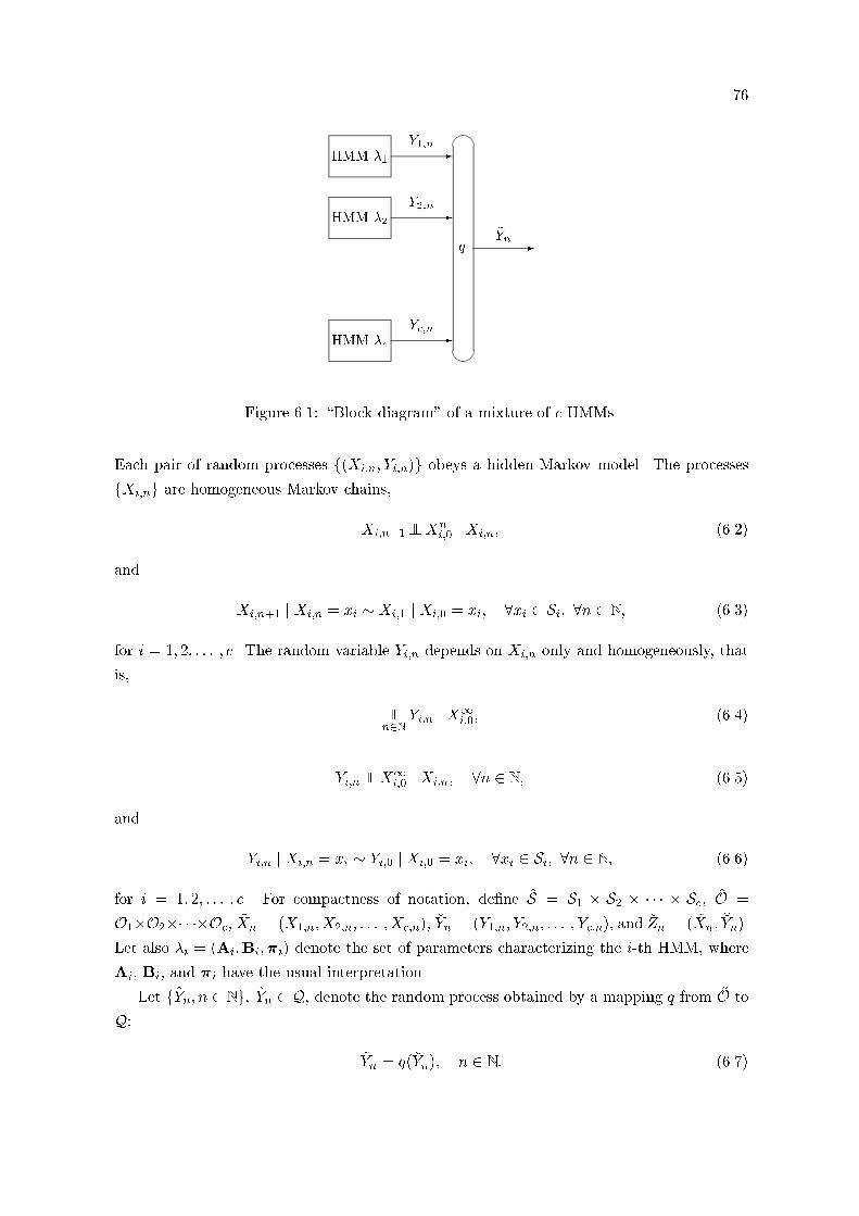
76
HMM �1
HMM �2
.
.
.
HMM �c -
-
-
Yc;n
Y2;n
Y1;n
q -~Yn
Figure 6.1: \Block diagram" of a mixture of c HMMs.
Each pair of random processes f(Xi;n; Yi;n)g obeys a hidden Markov model. The processes
fXi;ng are homogeneous Markov chains,
Xi;n+1??Xni;0 j Xi;n; (6.2)
and
Xi;n+1 j Xi;n = xi � Xi;1 j Xi;0 = xi; 8xi 2 Si; 8n 2 N; (6.3)
for i = 1; 2; : : : ; c. The random variable Yi;n depends on Xi;n only and homogeneously, that
is,
??n2N
Yi;n j X1i;0; (6.4)
Yi;n??X1i;0 j Xi;n; 8n 2 N; (6.5)
and
Yi;n j Xi;n = xi � Yi;0 j Xi;0 = xi; 8xi 2 Si; 8n 2 N; (6.6)
for i = 1; 2; : : : ; c. For compactness of notation, de�ne ~S = S1 � S2 � � � � � Sc, ~O =
O1�O2�� � ��Oc, ~Xn = (X1;n;X2;n; : : : ;Xc;n), �Yn = (Y1;n; Y2;n; : : : ; Yc;n), and �Zn = ( ~Xn; �Yn).
Let also �i = (Ai;Bi;�i) denote the set of parameters characterizing the i-th HMM, where
Ai, Bi, and �i have the usual interpretation.
Let f ~Yn; n 2 Ng, ~Yn 2 Q, denote the random process obtained by a mapping q from ~O to
Q:
~Yn = q( �Yn); n 2 N: (6.7)
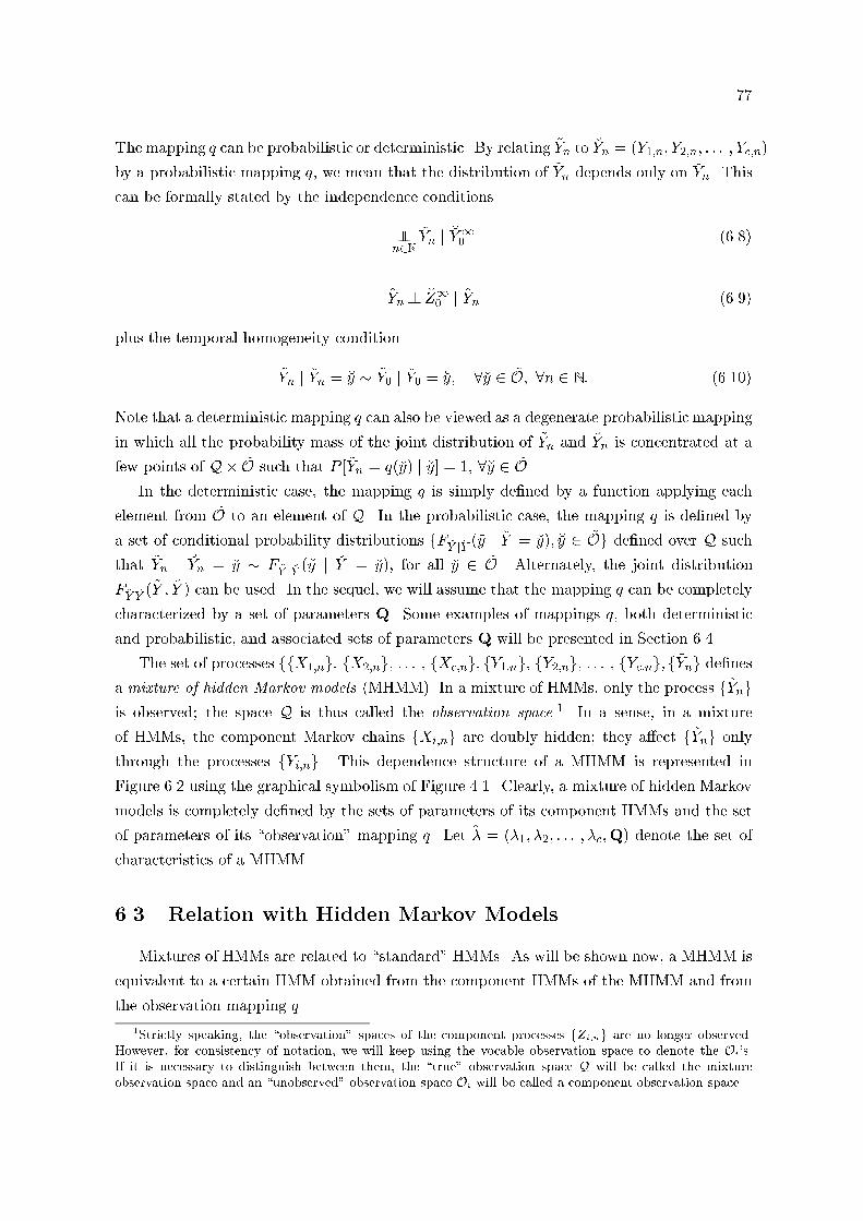
77
The mapping q can be probabilistic or deterministic. By relating ~Yn to �Yn = (Y1;n; Y2;n; : : : ; Yc;n)
by a probabilistic mapping q, we mean that the distribution of ~Yn depends only on �Yn. This
can be formally stated by the independence conditions
??n2N
~Yn j �Y10 (6.8)
~Yn?? �Z10 j ~Yn (6.9)
plus the temporal homogeneity condition
~Yn j �Yn = �y � ~Y0 j �Y0 = �y; 8�y 2 ~O; 8n 2 N: (6.10)
Note that a deterministic mapping q can also be viewed as a degenerate probabilistic mapping
in which all the probability mass of the joint distribution of ~Yn and �Yn is concentrated at a
few points of Q� ~O such that P [ ~Yn = q(�y) j �y] = 1, 8�y 2 ~O.In the deterministic case, the mapping q is simply de�ned by a function applying each
element from ~O to an element of Q. In the probabilistic case, the mapping q is de�ned by
a set of conditional probability distributions fF ~Y j �Y (~y j �Y = �y); �y 2 ~Og de�ned over Q such
that ~Yn j �Yn = �y � F ~Y j �Y (~y j �Y = �y), for all �y 2 ~O. Alternately, the joint distribution
F ~Y �Y (~Y ; �Y ) can be used. In the sequel, we will assume that the mapping q can be completely
characterized by a set of parameters Q. Some examples of mappings q, both deterministic
and probabilistic, and associated sets of parameters Q will be presented in Section 6.4.
The set of processes ffX1;ng, fX2;ng, : : : , fXc;ng; fY1;ng, fY2;ng, : : : , fYc;ng; f ~Yng de�nesa mixture of hidden Markov models (MHMM). In a mixture of HMMs, only the process f ~Yngis observed; the space Q is thus called the observation space.1 In a sense, in a mixture
of HMMs, the component Markov chains fXi;ng are doubly hidden; they a�ect f ~Yng onlythrough the processes fYi;ng. This dependence structure of a MHMM is represented in
Figure 6.2 using the graphical symbolism of Figure 4.1. Clearly, a mixture of hidden Markov
models is completely de�ned by the sets of parameters of its component HMMs and the set
of parameters of its \observation" mapping q. Let ~� = (�1; �2; : : : ; �c;Q) denote the set of
characteristics of a MHMM.
6.3 Relation with Hidden Markov Models
Mixtures of HMMs are related to \standard" HMMs. As will be shown now, a MHMM is
equivalent to a certain HMM obtained from the component HMMs of the MHMM and from
the observation mapping q.
1Strictly speaking, the \observation" spaces of the component processes fZi;ng are no longer observed.
However, for consistency of notation, we will keep using the vocable observation space to denote the Oi's.
If it is necessary to distinguish between them, the \true" observation space Q will be called the mixture
observation space and an \unobserved" observation space Oi will be called a component observation space.

78
6 6 6 6
- - -X1;0 X1;1 X1;2 X1;3
Y1;0 Y1;1 Y1;2 Y1;3
� � �
6 6 6 6
- - -X2;0 X2;1 X2;2 X2;3
Y2;0 Y2;1 Y2;2 Y2;3
� � �
� � � �6 6 6 6
~Y0 ~Y1 ~Y2 ~Y3� � �
observation veil
Figure 6.2: Conditional independence structure of a mixture of two HMMs.
Theorem 6.1 The pair of random processes f ~Zn = ( ~Xn; ~Yn); n 2 Ng extracted from of mix-
ture of hidden Markov models de�nes a hidden Markov model with Markov state process f ~Xngand observation process f ~Yng.
Proof. We need to show that the processes f ~Xng and f ~Yng obey the properties of a hidden
Markov model: the Markov property of the hidden process,
~Xn+1?? ~Xn0 j ~Xn; (6.11)
and the homogeneity of the Markov chain, the conditional independence of the observations
given the states,
??n2N
~Yn j ~X10 ;
~Yn?? ~X10 j ~Xn (6.12)
and the homogeneity of the observation given the states,
~Yn j ~Xn = ~x � ~Y0 j ~X0 = ~x; 8~x 2 ~S; 8n 2 N: (6.13)
The Markov property (6.11) and the homogeneity of the Markov chain follow trivially from
the Markov property of the processes fXi;ng, their homogeneity, and their independence
(6.1). The last property (6.13) is a direct consequence of the homogeneity property of the
components HMMs (6.6) and from their independence (6.1). The second property requires a
little more work. Showing (6.12) is equivalent to show
~Yn?? ~X10 j ~Xn (6.14)

79
and
~Yn?? ~Ym j ~Xn; 8m 6= n: (6.15)
From (6.4){(6.5), (6.1), and (6.8), we have, respectively,
�Yn?? ~X10 j ~Xn; (6.16)
and
~Yn?? ~X10 j �Yn; ~Xn: (6.17)
But (6.16) and (6.17) together are equivalent to ~X10 ?? �Yn; ~Yn j ~Xn which implies (6.14). We
have �Yn?? �Ym j ~Xn, 8m 6= n, from (6.4){(6.5) and (6.1), and �Yn?? ~Ym j �Ym, 8m 6= n. We
deduce �Yn?? �Ym; ~Yn j ~Xn, 8m 6= n. Combining the last expression with ~Yn?? ~Ym j �Yn; ~Xn, we
get �Yn; ~Yn?? ~Ym j ~Xn, 8m 6= n, which implies (6.15). This concludes the proof. �
Corollary 6.1 The pair of random processes f ~Xng and f �Yng extracted from a mixture of
hidden Markov models de�nes a hidden Markov model with state process f ~Xng, ~Xn 2 ~Sobservation process f �Yng, �Yn 2 ~O.
Proof. Simply note that if Q = ~O and q is the identity mapping, then ~Yn = �Yn. Theorem 6.1
yields then directly the corollary. �
The HMM equivalent to a MHMM can be de�ned from the speci�cation of the component
HMMs and of the observation mapping q. Recalling that A` = (a`;ij), a`;ij = P [X`;n+1 = j jX`;n = i], and using the independence property of the component HMMs (6.1), the transition
probabilities of the homogeneous Markov process f ~Xng are given by
P [ ~Xn = ~| j ~Xn�1 = ~{] =cY`=1
P [X`;n = i` j X`;n�1 = j`]
= a1;i1j1a2;i2j2 � � � ac;icjc= ~a~{~|; (6.18)
with ~{ = (i1; i2; : : : ; ic) 2 ~S and ~| = (j1; j2; : : : ; jc) 2 ~S. Let ~A = (~a~{~|), ~{; ~| 2 ~S be a 2c-order
tensor playing the role of the \transition matrix" for the Markov process f ~Xng. The elementsof ~A are given by (6.18). In more compact form, we can write
~A = A1 A2 � � �Ac; (6.19)
where denotes tensor product.2 Similarly, the initial state distribution on ~S can be obtainedfrom the initial state distributions of the component processes by
�~{ = P [ ~X0 = ~{]
=cY`=1
P [X`;0=i` ]
= �1;i1�2;i2 � � � �c;ic; (6.20)
2Here, the tensor product operation should be understood elementwise in the sense of (6.18).
80
with ~{ = (i1; i2; : : : ; ic) 2 ~S, or, in tensor notation,
~� = (~�~{)
= �1 �2 � � � �c: (6.21)
Remark 6.1 Instead of introducing a tensor notation for the initial and transition proba-
bilities of f ~Xng, it is possible to work with matrices and vectors. The Cartesian product of
state spaces ~S is �nite since all the component state spaces Si are �nite. It can therefore be
identi�ed with a subset of the integer,
~S � f1; 2; : : : ; ~Mg; ~M = # ~S =cYi=1
Mi (6.22)
with Si = f1; 2; : : : ;Mig. The one-to-one equivalence can be established, for example, by
~x = (x1; x2; : : : ; xc) � ~{, xi 2 Si, ~{ 2 f1; 2; : : : ; ~Mg, with
~{ =c�1X`=1
24(x` � 1)
cYk=`+1
Mk
35+ xc:
By mapping the Cartesian product space ~S = S1�S2�� � ��Sc to f1; 2; : : : ; ~Mg, it becomespossible to de�ne a ~M � ~M transition matrix ~A and a ~M -dimensional initial probability
vector ~� for f ~Xng. Equations (6.19) and (6.21) should then be interpreted as Kronecker
products of matrices and vectors instead of tensor products.
Using again the independence property of the component HMMS (6.1), it is straightfor-
ward to obtain the state conditional distributions of �Yn given ~Xn from the state conditional
distributions of the component processes. Let FYijXidenote the state conditional distribution
of Yi;n given Xi;n, i.e.,
Yi;n j Xi;n = xi � FYijXi(yijxi); 8xi 2 Si; 1 � i � c:
The state conditional distributions of the combination of HMMs
�Yn j ~Xn = ~x � F �Y j ~X(�yj~x); 8~x 2 ~S;
is simply
F �Y j ~X(�yj~x) =cYi=1
FYijXi(yijxi); ~x = (x1; x2; : : : ; xc) 2 ~S:
The state conditional distribution of ~Yn given ~Xn can be computed using the independence
and homogeneity properties of MHMMs (6.8){(6.10) by \integrating out" the variable �Yn. In
the most general form, we can write
F ~Y j ~X(~yj~x) =Z~OF ~Y j �Y (~yj�y)dF �Y j ~X(�yj~x): (6.23)

81
Like in the standard HMM case, let Bi denote the set of parameters characterizing the
state conditional distributions of Yi;n given Xi;n. Then, the state conditional distribution of
�Yn given ~Xn is de�ned by ~B = (B1;B2; : : : ;Bc). The state conditional distribution of ~Yn
given ~Xn can then be characterized by a set of parameters ~B computed from �B and Q. Going
any further requires the postulation of a particular form for the state conditional distributions
of the Yi;n and for the observation mapping q (and associated distributions). Some examples
will be given in the next section.
Thus, the HMM equivalent to a MHMM is completely de�ned by the set of parameters
~�0 = ( ~A; ~B; ~�) which can be computed from the set of parameters of the MHMM ~� =
(�1; �2; : : : ; �c;Q). From now on, we will drop the prime to denote the equivalent HMM
parameter set. We will use ~� to mean either the parameter set of a MHMM or the parameter
set of its equivalent HMM.
The HMM equivalent to a MHMM inherits from the properties of its component HMMs.
If the component HMMs fYi;ng are stationary and ergodic, then the observed process f ~Yngis also stationary and ergodic.
Theorem 6.2 Let ~Yn be a mixture of c HMMs f(X1;n; Y1;n)g, f(X2;n; Y2;n)g, : : : , f(Xc;n; Yc;n)g.If the Markov chains fXi;ng are stationary and ergodic (i.e., the processes fYi;ng are station-ary and ergodic), then f ~Yng is stationary and ergodic.
Proof. We will prove that the Markov chain f ~Xn = (X1;n;X2;n; : : : ;Xc;n)g is stationaryand ergodic if the Markov chains fXi;ng are stationary and ergodic. The stationarity and
ergodicity of ~Yn will then follow directly as a corollary of Theorem 2.3.
Denote by Ai and ��i the transition matrix and the initial stationary distribution associ-
ated with fXi;ng. Let~�� = ��1 ��2 � � � ��c ;
and
~A = A1 A2 � � �Ac:
By the mixed-product property of , we have
~�� = (��1A1) (��2A2) � � � (��cAc)
= (��1 ��2 � � � ��c) (A1 A2 � � �Ac)
= ~�� ~A:
Thus, ~�� is a stationary distribution of f ~Xng. The state space ~S of f ~Xng being �nite, it
is su�cient to show irreducibility and aperiodicity to have ergodicity. Irreducibility follows
from the irreducibility of the component Markov chains fXi;ng by observing that i` $ j`,
8i`; j` 2 S`, ` = 1; 2; : : : ; c implies ~{ = (i1; i2; : : : ; ic) $ ~| = (j1; j2; : : : ; jc), 8~{; ~| 2 ~S.
82
Similarly, aperioricity of f ~Xng follows from the aperiodicity of the component Markov chains
fXi;ng and their independance. The Markov chain f ~Xng is thus stationary and ergodic. �
6.4 Types of MHMMs
There are two particular types of mixtures of HMMs that will be treated in more details
in the next two chapters: mixtures of discrete HMMs and mixtures of continuous HMMs.
6.4.1 Mixtures of Discrete HMMs
In a mixture of discrete hidden Markov models (MDHMM), both the component HMMs
and the mixture have discrete observation spaces, i.e., Oi � N andQ � N. If all these discrete
spaces are �nite, it can be assumed without loss of generality, as in the single DHMM case of
Section 2.1.1, that the component observation spaces Oi can be identi�ed with f1; 2; : : : ; Lig,Li = #Oi, i = 1; 2; : : : ; c, and that the mixture observation space Q can be identi�ed with
f1; 2; : : : ; Qg, Q = #Q. We consider only the non-parametric case where the component
HMM state conditional distributions are de�ned by stochastic matrices of emission probabil-
ities Bi = (bi;jk), 1 � i � c, with
bi;jk = P [Yi;n = k j Xi;n = j]; 1 � j �Mi; 1 � k � Li; (6.24)
and where the probabilistic mapping q is de�ned by the order c + 1 tensor of observation
probabilities Q = (q~{j),
q~{j = P [ ~Yn = j j ~Yn = ~{]; ~{ 2 ~O; 1 � j � Q: (6.25)
Mixtures of discrete HMMs will be the subject of more detailed treatment in Chapter 7.
The HMM equivalent to a MDHMM can be easily computed. It is straightforward to
see that the equivalent HMM with state space ~S and observation space Q is also a discrete
HMM. Its state transition probabilities ~A and initial state probabilities ~� are given by (6.19)
and (6.21). Its state conditional distributions are de�ned by the order c+1 tensor ~B = (~b~{j),
~{ 2 ~S, 1 � j � Q, where
~b~{j = ~b~{(j)
= P [ ~Yn = j j ~Xn = ~{]
=X~k2 ~O
P [ ~Yn = j j �Yn = ~k]P [ �Yn = ~k j ~Xn = ~{]
=X~k2 ~O
q~kj�b~{~k (6.26)
with
�b~{~k = b1;i1k1b2;i2k2 � � � bc;ickc (6.27)

83
Gathering the emission probabilities of (6.27) into an order 2c tensor �B = (�b~{~k), we get
�B = B1 B2 � � � Bc; (6.28)
It is possible to summarize the relations de�ning ~B by
~B = Q �B: (6.29)
Note that the comments of Remark 6.1 also apply to the state conditional distributions of
the DHMM equivalent to a MDHMM. That is, it is possible to replace the utilization of
tensors and tensor products with the utilization of matrices and Kronecker matrix products
by mapping the Cartesian product space ~O onto the subset of the integers f1; 2; : : : ; ~L,~L =
Qci=1 Li. In this case, ~Q becomes a ~L � Q stochastic matrix, �B becomes a ~M � ~L
stochastic matrix, ~B becomes a ~M � Q stochastic matrix, and (6.28) and (6.29) should be
interpreted as a Kronecker product of matrices and as a standard matrix product, respectively.
6.4.2 Mixtures of Continuous HMMs
In amixture of continuous hidden Markov models (MCHMM), both the component HMMs
and the mixture have continuous observation spaces, i.e., Oi � Rdi and Q � R
~d . As usual
with continuous HMMs, the state conditional probability density functions will belong to a
parametric family,
bi;j(yi) = pYi(y; �i;j) = fi(yi; �i;j); j 2 Si; y 2 Oi; �i;j 2 �i (6.30)
and the parameters �i;j will be gathered in matrices Bi = (�i;1; �i;2; : : : ; �i;Mi), for i =
1; 2; : : : ; c. The observation mapping q will be assumed to be a deterministic point to point
mapping ~y = q(�y) , i.e.,
q : ~O ! Q; �y ! q(�y):
Let Q be some set of parameters describing q (see the example below). If we want to make
explicit the dependence of q on Q, we will write ~y = qQ(�y). Note that for a MCHMM, the
Cartesian product space ~O reduces to the �d-dimensional Euclidean space R�d with �d =
Pci=1 di.
The HMM equivalent to a MCHMM can be easily computed. It is straightforward to see
that the equivalent HMM with state space ~S and observation space Q is a continuous HMM.
Its state transition probabilities ~A and initial state probabilities ~� are given by (6.19) and
(6.21). Its state conditional distributions are de�ned by the probability density functions
~b~{(~y) =
Z~y=q(�y)
�b~{(�y)d�y; ~y 2 Q; ~{ 2 ~S; (6.31)
where
�b~{(�y) = b1;i1(y1)b2;i2(y2) � � � bc;ic(yc); ~y 2 ~O; ~{ 2 ~S: (6.32)

84
Depending on the form of the state conditional distributions bi;j(yi) and on the observa-
tion mapping q, (6.31) may or may not yield a closed parametric form for ~b~{(~y). If such a
parametric form exists,
~b~{(~y) = p ~Y (~y;~�~{) = ~f(~y; ~�~{); ~�~{ 2 ~�; (6.33)
and the state conditional distributions of the equivalent HMM will be characterized by ~B =
(~�~{), ~{ 2 ~S with ~�~{ function of �1;i1 ; �2;i2 ; : : : ; �c;ic and Q. An example of MCHMM for which
the equivalent HMM admits the same parametric form as the components HMMs is the linear
mixture of Gaussian CHMMs.
Linear Mixtures of Gaussian CHMMs
Consider the case where O1 = O2 = � � � = O2 = Q = Rd , the state conditional probabili-
ties are Gaussian pdfs, and the mapping q is linear. That is, for the state conditional pdfs,
we have
bi;j(yi) =1
(2�)d=2j�i;jj1=2exp
��12(yi � �i;j)0��1
i;j (yi ��i;j)�; yi 2 Rd ; 1 � j �Mi;
(6.34)
and �i;j = (�i;j;�i;j). For the observation mapping, we have
~Yn = qQ( �Yn)
= q1Y1;n + q2Y2;n + � � �+ qcYc;n (6.35)
where Q = (q1; q2; : : : ; qc) 2 Rc .Furthermore, the linearity of q in Yi;n implies that the state conditional pdfs of ~Yn
in the equivalent HMM are also Gaussian. Conditionally on ~Xn, the random variables
Y1;n; Y2;n; : : : ; Yc;n are independent Gaussian random variables. We thus have
~b~{(~y) =1
(2�)d=2j ~�j1=2 exp��12(~y � ~�~{)
0 ~��1
~{ (~y � ~�~{)
�; ~{ 2 ~S; (6.36)
with
~�~{ = q1�1;i1 + q2�2;i2 + � � �+ qc�c;ic; (6.37)
~�~{ = q21�1;i1 + q22�2;i2 + � � �+ q2c�c;ic: (6.38)
Mixtures of continuous HMMs, and, particularly, linear mixtures of Gaussian HMMs, will
be the subject of more detailed treatment in Chapter 8. Some applications of this model will
be presented in the last section of this chapter.
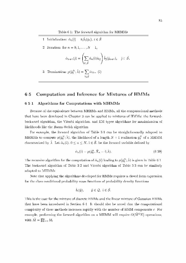
85
Table 6.1: The forward algorithm for MHMMs.
1. Initialization: ~�0(~{) = ~�~{~b~{(~y1), ~{ 2 ~S.
2. Iteration: for n = 0; 1; : : : ; N � 1,
~�n+1(~|) =
0@X~{2 ~S
~�n(~{)~a~{~|
1A~b~|(~yn+1); ~| 2 ~S:
3. Termination: p(~yN0 ;~�) =
X~{2 ~S
~�N�1(~{).
6.5 Computation and Inference for Mixtures of HMMs
6.5.1 Algorithms for Computations with MHMMs
Because of the equivalence between MHHMs and HMMs, all the computational methods
that have been developed in Chapter 3 can be applied to mixtures of HMMs: the forward-
backward algorithm, the Viterbi algorithm, and EM types algorithms for maximization of
likelihoods like the Baum-Welsh algorithm.
For example, the forward algorithm of Table 3.1 can be straightforwardly adapted to
MHMMs to compute p(~yN0 ;~�), the likelihood of a length N + 1 realization ~yN0 of a MHMM
characterized by ~�. Let ~�n(~{), 0 � n � N , ~{ 2 ~S, be the forward variable de�ned by
~�n(~{) = p(~yn0 ;~Xn = ~{; ~�): (6.39)
The recursive algorithm for the computation of ~�n(~{) leading to p(~yN0 ;
~�) is given in Table 6.1.
The backward algorithm of Table 3.2 and Viterbi algorithm of Table 3.3 can be similarly
adapted to MHMMs.
Note that applying the algorithms developed for HMMs requires a closed form expression
for the class conditional probability mass functions of probability density functions
~b~{(~y); ~y 2 Q; ~{ 2 ~S:
This is the case for the mixture of discrete HMMs and the linear mixture of Gaussian HMMs
that have been introduced in Section 6.4. It should also be noted that the computational
complexity of these methods increases rapidly with the number of HMM components c. For
example, performing the forward algorithm on a MHMM will require O( ~M2N) operations,
with ~M =Qci=1Mi.

86
6.5.2 Filtering of MHMMs
There are some inference issues speci�c to MHMMs that cannot be solved by directly
adapting HMM methods. One such issue is the estimation of the component HMMs observa-
tion processes fYi;ng, 1 � i � c, from samples of the mixture process f ~Yng. This estimationproblem is known as the �ltering or smoothing problem. Let ~yN0 be a length N + 1 sample
of the observation process of MHMM characterized by ~�. The minimum mean square er-
ror (MMSE) and maximum a posteriori (MAP) estimators of the component processes Yi;n,
1 � i � c, 1 � n � N , are derived below.
6.5.2.1 MMSE Estimator
The MMSE estimator of Yi;n given ~yn0 is de�ned by
yi;n = E[Yi;n j ~yN0 ]: (6.40)
Using the properties of mixtures of HMMs, we get
yi;n =X~|2 ~S
P [ ~Xn = ~| j ~yN0 ]E[Yi;n j ~yN0 ; ~Xn = ~|]
=X~|2 ~S
~ n(~|)E[Yi;n j ~Yn = ~yn; ~Xn = ~|] (6.41)
where the a posteriori state probability ~ n(~|) = P [ ~Xn = ~| j ~yN0 ] can be computed using the
forward-backward algorithm. The computation of E[Yi;n j ~yn; ~Xn = ~|] can be performed very
easily for some type of HMMs when a closed form expression is available for the means of
the state conditional distribution given ~Yn = ~yn, viz. p(yi;n j ~yn; ~Xn = ~|).
For example, for the linear mixtures of Gaussian CHMMs of Section 6.4.2, the state condi-
tional pdfs given ~Yn = ~yn are Gaussian. This results directly from the fact that, conditionally
on the composite state ~Xn, the variables Y1;n, Y2;n, : : : , Yc;n, and ~Yn are Gaussian and related
by a linear relation. The distribution of Yi;n j ~Yn = ~yn; ~Xn = ~| is thus Gaussian with mean
vector and covariance matrix given by (Anderson 1984)
�ij~yn;~| = E[Yi;n j ~yn; ~Xn = ~|]
= �i +�i~��1~| (~yn � ~�~|); (6.42)
where ~�~| = qj1�j1 + qj2�j2 + � � � + qjc�jc and~�~| = q2j1�j1 + q2j2�j2 + � � �+ q2jc�jc , and
�ij~yn;~| = Cov(Yi;n j ~yn; ~Xn = ~|)
= �i ��i~��1�i (6.43)
From (6.41) and (6.42), we get for the MMSE estimator of Yi;n in the linear mixture of
Gaussian CHMM case the simple expression
yi;n =X~|2 ~S
~ n(~|)�ij~yn;~|: (6.44)

87
6.5.2.2 MAP Estimator
The MAP estimator of Yi;n is de�ned by
yi;n = arg maxyi;n2Oi
p(yi;nj~yN0 ); (6.45)
Note that
p(yi;nj~yN0 ) =X~|2 ~S
P [ ~Xn = ~| j ~yN0 ]p(yi;nj~yN0 ; ~Xn = ~|)
=X~|2 ~S
~ n(~|)p(yi;nj~yn; ~Xn = ~|) (6.46)
For mixtures of discrete HMMs, the maximization of (6.45) over Oi = f1; 2; : : : ; Lig isusually easy. For example, for the non-parametric MDHMM of Section 6.4.1, it is a matter
of trivial algebra to show that
p(yi;n j ~yn; ~Xn = ~|)
=1
P [ ~Yn = ~yn]
X�k2 ~O
ki=yi;n
P [ ~Yn = ~yn j �Yn = �k; ~Xn = ~|]P [ �Yn = �k j ~Xn = ~|]
=
X�k2 ~O
ki=yi;n
q�k~yn~b~x�k
X�k2 ~O
q�k~yn~b~x�k
; (6.47)
where �k = (k1; k2; : : : ; kc). Direct maximization of (6.45) is possible with O( ~MMi) opera-
tions.
For mixtures of continuous HMMs, direct maximization of (6.45) is usually not possible;
it is necessary to resort to numerical optimization procedures. The structure of the prob-
lem suggests naturally the utilization of an EM-type algorithm. The application of the EM
algorithm to the maximization of (6.45) requires some preliminary work since the \parame-
ter" that has to be estimated, yi;n is a realization of a random variable and the \likelihood
function" p(yi;nj~yN0 ) is not a true likelihood with respect to the \parameter" yi;n and the
\incomplete data" ~Y N0 . First, observe that
arg maxyi;n2Oi
p(yi;nj~yN0 ) = arg maxyi;n2Oi
p(yi;n; ~yN0 );
where both distributions are considered as deterministic functions of yi;n. Let ( ~YN0 ; ~Xn) be
the \complete data" and de�ne the associated auxiliary function by
Q(�yi;n; yi;n) = Ehln p( ~Y N
0 ; ~Xn; �yi;n) j ~yN0 ; yi;ni: (6.48)
Since
ln p( ~Y N0 ; ~Xn; �yi;n) = ln p(�yi;nj ~Y N
0 ; ~Xn)� ln p( ~Y N0 ; ~Xn);

88
the maximization of Q(�yi;n; yi;n) with respect to �yi;n is equivalent to the maximization of
Q0(�yi;n; yi;n) = Ehln p(�yi;nj~yN0 ; ~Xn) j ~Y N
0 = ~yN0 ; yi;ni
=X~|2 ~S
P [ ~Xn = ~|j~yN0 ; yi;n] ln p(�yi;nj~yn; ~Xn = ~|): (6.49)
The EM algorithm for MAP estimation is thus
1. E-step: determine Q0(�yi;n; yi;n),
2. M-step: choose �yi;n 2 arg max�yi;n2Oi
Q0(�yi;n; yi;n),
where yi;n denotes the current estimate and �yi;n denotes the next estimate. The \posterior"
probabilities P [ ~Xn = ~| j ~Y N0 = ~yN0 ; Yi;n = yi;n] in Q0(�yi;n; yi;n) can generally be computed
e�ciently by the forward-backward formulae by observing that
P [ ~Xn = ~|j~yN0 ; yi;n] =~ n(~|)p(yi;nj~yN0 ; ~Xn = ~|)X
~k2 ~S
~ n(~k)p(yi;n~yN0 ;
~Xn = ~k)= �n(~|; yi;n): (6.50)
The M-step usually admits an analytical solution and the EM algorithm reduces to simple
re-estimation formulae. For instance, for a linear mixture of Gaussian CHMMs, it is not
di�cult to show that
�yi;n =X~|2 ~S
�n(~|; yi;n)�ij~yn;~|;
where �ij~yn;~| is given by (6.42). An alternative derivation of this MAP algorithm and
an application to a two components linear mixture of Gaussian CHMMs can be found in
(Ephraim 1992a).
6.5.3 Decomposition of MHMMs
In Section 5.1.1, the classi�cation problem for HMMs was de�ned. It was summarized
as follows: given a �nite dictionary of possible hidden Markov models and a realization yN0
of an unknown HMM from the dictionary, decide on the HMM from the dictionary from
which yN0 has been sampled. The decomposition of a mixture of HMMs can be viewed as a
generalization of the concept of classi�cation of Section 5.1.1. In the decomposition problem,
multiple HMMs from the dictionary can be selected and they are not observed directly but
through some (possibly probabilistic) mapping q. The problem becomes: given a sample ~yN0
of an unknown MHMM, a dictionary of possible components, and an observation mapping
q, �nd the elements from the dictionary that compose the MHMM from which ~yN0 has been
sampled.
Let � = f�1; �2; : : : ; �cg denote a dictionary of c distinct HMMs, with Si and Oi the stateand observation spaces associated with �i. Let � denote an index set for �, i.e., a subset of
indices
� � f1; 2; : : : ; cg:

89
HMM �c
Yc;n-
.
.
.
HMM �2
Y2;n-
HMM �1
Y1;n-
�
q -~Yn
Figure 6.3: \Block diagram" for the composition of a MHMM from a dictionary of HMMs
and an observation mapping.
We will write � = f�1; �2; : : : ; �rg, r = #�. Let
~S� = S�1 � S�2 � � � � � S�r
and
~O� = O�1 �O�2 � � � � � O�rbe the Cartesian state space and Cartesian component observation space associated with �.
Let q : ~O ! Q be a (possibly probabilistic) observation mapping. Assume that the mapping q
is de�ned such that it can be restricted to ~O� � ~O and let q� : ~O� ! Q denote this restriction.
For example, if the mapping q is probabilistic, the restriction q� can be obtained by taking
the marginal of the joint distribution F ~Y �Y (~y; y1; y2; : : : ; yc) that de�nes q with respect to
~y; y�1 ; y�2 ; : : : ; y�r . If Q denotes the set of parameters that de�nes q, let Q� denote the set
of parameters that de�nes q�; in many cases, Q� � Q. Clearly, to each set of indices � is
associated a MHMM de�ned by ~�� = (��1 ; ��2 ; : : : ; ��c ;Q�). The composition of a MHMM
from a dictionary of HMMs � and an observation mapping q is summarized in Figure 6.3.
The mixture of HMMs decomposition problem can be stated formally as: given a dic-
tionary of HMMs �, an observation mapping q (admitting restrictions), and a sample ~yN0
of a MHMM process f ~Yng obtained by composition of some HMMs in �, �nd which HMMs
from � compose f ~Yng, i.e., �nd the index set � associated with f ~Yng. The number of ele-
ments HMMs from the dictionary composing f ~Yng (the cardinal of �) is unknown a priori.
In layman's terms, the problem is �nding the \switches" that are \on" in Figure 6.3.
As for HMM classi�cation, the problem can be cast in a decision theoretic framework and
the optimal Bayes decision rule can be obtained easily. To each possible index set � corre-
sponds a MHMM ~��, and to each MHMM ~�� corresponds a hypothesis for the distribution of
~Y N0 . Thus, �nding the components of the MHMM can be written as the multiple hypotheses

90
test
H� : ~Y N0 � p(~yN0 ; ~��); 8� 2 f1; 2; : : : ; cg:
where the decision has to be made from a single sample ~yN0 . Let P [~��] denote the a priori
probability that the hypothesis � is true. The Bayes decision rule with minimum probability
of error
!�(~yN0 ) : QN+1 ! �; (6.51)
where � denotes the set of all subsets of f1; 2; : : : ; cg is given by
!�(~yN0 ) = argmax�2�
P [~��j~yN0 ]
= argmax�2�
p(~yN0 ;~��)P [~��]: (6.52)
The likelihoods p(~yN0 ;~��) can be computed by the forward-backward algorithm as explained
in Section 6.5.1.
One of the main di�culties encountered when implementing the Bayes decision rule for
mixture decomposition is the exponential explosion of the number of hypotheses that have to
be tested. For a dictionary of size c, there are c! di�erent subsets � and associated mixture
hypotheses. Exhaustive computation of the likelihoods for all hypotheses becomes rapidly
intractable, even on a powerful computer. It is then necessary to resort to approximations
and sub-optimal strategies, some of which will be developed in Chapter 7 and Chapter 8.
Note that the \standard" HMM classi�cation problem can be viewed as a special case
of the HMM decomposition problem where only one element from the dictionary � can be
present (i.e., only one switch in Figure 6.3 can be \on" at a time), O� = O1 = O2 =
� � � = Oc = O, and the mapping q is the identity mapping with the proper restriction to
Q = O� = O.
6.6 Applications and Related Models
6.6.1 Environmental Sound Recognition
A typical application of MHMM is the recognition of environmental sound sources when
multiple sound sources can be present simultaneously, as explained in Chapter 1. This
application motivated the introduction of the concept of MHMMs (Couvreur, Fontaine &
Leich 1996).
Hidden Markov models can be applied to the classi�cation of single environmental sound
sources, such as cars, helicopter, factories, etc. (Woodard 1992). The classi�cation scheme
used is the same as the one used in speech recognition. The acoustical signal recorded at
a microphone is pre-processed and turned into a sequence of variables fYng (discrete or
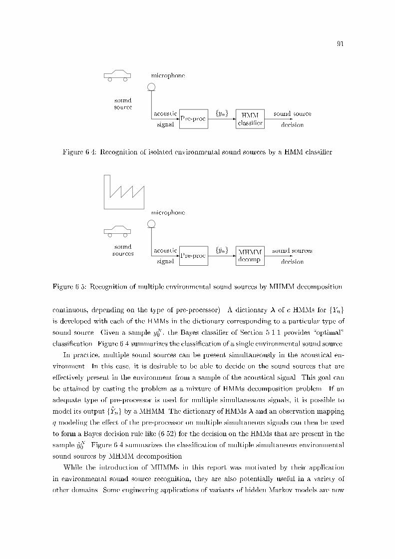
91
sound
source
microphone
acoustic-signal
Pre-proc.
fyng- HMM
classi�er
-sound source
decision
Figure 6.4: Recognition of isolated environmental sound sources by a HMM classi�er.
sound
sources
microphone
acoustic-signal
Pre-proc.
f~yng- MHMM
decomp.
-sound sources
decision
Figure 6.5: Recognition of multiple environmental sound sources by MHMM decomposition.
continuous, depending on the type of pre-processor). A dictionary � of c HMMs for fYngis developed with each of the HMMs in the dictionary corresponding to a particular type of
sound source. Given a sample yN0 , the Bayes classi�er of Section 5.1.1 provides \optimal"
classi�cation. Figure 6.4 summarizes the classi�cation of a single environmental sound source.
In practice, multiple sound sources can be present simultaneously in the acoustical en-
vironment. In this case, it is desirable to be able to decide on the sound sources that are
e�ectively present in the environment from a sample of the acoustical signal. This goal can
be attained by casting the problem as a mixture of HMMs decomposition problem. If an
adequate type of pre-processor is used for multiple simultaneaous signals, it is possible to
model its output f ~Yng by a MHMM. The dictionary of HMMs � and an observation mapping
q modeling the e�ect of the pre-processor on multiple simultaneous signals can then be used
to form a Bayes decision rule like (6.52) for the decision on the HMMs that are present in the
sample ~yN0 . Figure 6.4 summarizes the classi�cation of multiple simultaneous environmental
sound sources by MHMM decomposition.
While the introduction of MHMMs in this report was motivated by their application
in environmental sound source recognition, they are also potentially useful in a variety of
other domains. Some engineering applications of variants of hidden Markov models are now

92
reviewed and their relation with our general mixture of HMMs model is discussed.
6.6.2 Speech Plus Noise HMMs
A model that can be viewed as a particular case of our MHMM has been proposed by
several authors in the speech processing literature for the processing of noisy speech. Let the
process f ~Yn; n 2 Ng, ~Yn 2 Rd , represent a noisy speech signal.3 If the noise is additive, we
have
~Yn = Y1;n + Y2;n (6.53)
where the processes fY1;ng and fY2;ng represent the clean speech signal and the perturbing
noise, respectively. If we assume that both the speech process fY1;ng and the noise process
fY2;ng can be modeled by CHMMs, the resulting model for the noisy speech f ~Yng is a linearmixture of two continuous HMMs. This model has been applied successfully to two speci�c
problems: speech enhancement and recognition of noisy speech.
6.6.2.1 Speech Enhancement
In speech enhancement, the goal is to \remove" the noise from the noisy speech signal
to retrieve the clean speech signal. In statistical parlance, \removing the noise" amounts
to the estimation of the speech process fY1;ng from observations of the noisy speech process
f ~Yng. Assuming that known hidden Markov models are available for the clean speech process
fY1;ng and the noise process fY2;ng, this is precisely the problem that has been treated in
Section 6.5.2. The MMSE and MAP estimators for linear mixtures of Gaussian processes
have been applied to speech enhancement in (Ephraim 1992a). The reader interested in more
details on HMM-based speech enhancement systems should consult Ephraim's (1992c) review
paper and the references therein.
6.6.2.2 Noisy Speech Recognition
Let us assume that a dictionary �1 of c1 word HMMs for the speech process fY1;ng and a
dictionary �2 of c2 noise HMMs for the noise process fY2;ng are available. Let � = �1 [ �2,c = c1 + c2. For simplicity, consider �rst the case where c2 = 1; that is, there is only one
type of noise. Given a sample of the noisy speech ~yN0 , �nding the word pronounced simply
amounts to a mixture of HMMs decomposition problem with the dictionary of HMMs � and
the linear observation mapping (6.53). The Bayes rule (6.52) can be applied with a set of
index hypotheses � restricted to the pairs of indices � = f�1; �2g corresponding to one element�1 from the word HMMs dictionary �1 and the single noise HMM from �2. The generalization
to multiple noise sources, and, possibly, multiple simultaneous speakers is straightforward.
3Possibly after some pre-processing of the acoustical signal (cf. Figure 1.3).

93
Several authors have applied variants of this scheme to the recognition of speech in noise
(Ephraim 1992b, Gales & Young 1992, Gales & Young 1993b, Gales & Young 1993a, Martin,
Shikano & Minami 1993, Minami & Furui 1995, Nakamura, Takiguchi & Shikano 1996, Varga
& Moore 1990, Wang & Young 1992).4 See also (Green, Cooke & Crawford 1995) or (Xu,
Fancourt & Wang 1996) for related techniques.
6.6.3 Multiple Object Tracking
Hidden Markov models have been proposed for object tracking in (White 1991, Streit &
Barret 1990, Xie & Evans 1993a, Frenkel & Feder 1995). The object tracked can be a mov-
ing target in radar/sonar or a time-varying FM carrier in communication. The unobserved
movement of the object to be tracked is modeled by a Markov chain. Imperfect observa-
tions of the trajectory of the object are made; these observations are assumed to obey the
conditions for a HMM. Tracking the object simply consists of using the Viterbi algorithm
to estimate its trajectory. Various authors have proposed to extend the method to multiple
simultaneous objects (White 1992, Xie & Evans 1991, Xie & Evans 1993b). Their extension
simply amounts to de�ning a mixture of HMMs model for the global evolution of the objects
and the observations; the Viterbi algorithm can then be applied to estimate the sequences of
hidden states.
4Other methods based on HMMs for noisy speech recognition have been proposed that can also be related
to MHMMs. They usually follow an ad hoc approach relying on speech-domain knowledge. For that reason,
they will not be discussed in this report. See (Rabiner & Juang 1993, Chapter 5{6) for some details and
references.

94
Chapter 7
Decomposition of Mixtures of
Discrete Hidden Markov Models
In this chapter and in the next one, we describe in some more details the application
of mixtures of HMMs to the classi�cation of simultaneous signals. As explained in Sec-
tion 6.5.3, such a problem occurs in environmental acoustics. While this application is the
main motivation for our interest for decomposition of mixtures of HMMs, many of the tech-
niques presented have potential applications in speech processing or in radar/sonar signal
processing.
The treatment in these last two chapters is less rigorous than in the previous ones. We
try to state the problem as precisely as possible and to suggest some solutions susceptible of
a practical application. Many of the results presented lack a complete theoretical analysis.
This part of the work is left for the future.
We start by formulating the classi�cation of mixtures of simultaneous signals in terms
of the decomposition of a mixture of discrete HMMs. The optimal solution obtained by the
Bayes classi�er is then described and some sub-optimal solutions with reduced computational
load are presented. We conclude this chapter by some preliminary numerical results.
7.1 Problem Formulation
Recall the formulation of the discrete HMM classi�cation problem for single signals (not
speci�cally for speech signals). Let fY (t); t 2 R+g, Y (t) 2 R
d , be the original \analog"
signal (considered as a continuous-time random process). This continuous-time process is
mapped by a pre-processor to a discrete-time process fYn; n 2 Ng, Yn 2 O � N0 , which is
modeled by a discrete HMM. Let � = f�1; �2; : : : ; �cg be a dictionary of possible hidden
Markov models for Yn. The classi�cation problem is: given a sample yN0 of fYng obtainedby pre-processing a �nite length sample of fY (t)g, �nd the HMM from � that models fYng.The optimal solution in the sense of minimal probability of error was shown in Section 5.1.1

95
-fy(t)g
Pre-proc. -fyng HMM
classi�er
-decision
Figure 7.1: Classi�cation of a single signal with HMMs.
to be the Bayes classi�er or Bayes decision rule (5.5). Figure 7.1 summarizes the single HMM
classi�cation scheme.
Let us assume that more than one signal can be present and that all that is observed is
their sum
~Y (t) =rXi=1
Yi(t);
where fYi(t)g, i = 1; 2; : : : ; r, denotes the individual signal. Let fYi;ng, Yi;n 2 Oi = O,be the processes that would be observed if each of the analog signals fYi(t)g was processedby the same pre-processor as in the single signal case. Again, let � = f�1; �2; : : : ; �cg bea dictionary of possible discrete hidden Markov models for the processes fYi;ng. As usual,
denote by Si the state space of the i-th model and by �i = (Ai;Bi;�i) its set of parameters.
The classi�cation problem for multiple simultaneous signals is simply: given a �nite length
sample of f ~Y (t)g, �nd the models from � that correspond to the components fYi(t)g in
f ~Y (t)g. If each signal fYi(t)g could be accessed and pre-processed separately, the optimal
solution would be the application of the Bayes decision rule (5.5) to each resulting sequences
yNi;0. In practice, all that is available is the sample of f ~Y (t)g, and this solution cannot be
applied. However, it seems intuitively sound to try to estimate Y Ni;0 , i = 1; 2; : : : ; r, from
the sample of f ~Y (t)g and then apply the Bayes decision rule to the resulting sequences of
estimates. This estimation can be performed by a special pre-processor for f ~Y (t)g. The
speci�c nature of the mixture pre-processor depends on the applications; some examples of
such pre-processors can be found in (Couvreur & Bresler 1995a, Couvreur & Bresler 1996, Xie
& Evans 1991, Xie & Evans 1993b, Green et al. 1995). Statistical modeling of the pre-
processor leads to a formulation of the classi�cation of simultaneous signals in terms of a
mixture decomposition problem (Couvreur et al. 1996).
For simplicity, assume that to each process fYi;ng corresponds a distinct model in �
(implying r � c). Thus, there are at most c components in f ~Y (t)g. The exact number of
components r is unknown a priori. Let f ~Yng, ~Yn 2 Q, denote the output of the mixture
pre-processor and let f �Yn = (Y1;n; Y2;n; : : : ; Yr;n)g, �Yn 2 ~O = Or � Oc, be the process
gathering the outputs of the \single signal" pre-processors. Ideally, we would like Q = Orand ~Yn = �Yn. Practically, the mixture pre-processor has limitations dictated by the nature
of the application. For instance, r is unknown a priori and can only be guessed at by the
pre-processor; the mixture pre-processor output will always be de�ned up to a permutation
of the components (that is, the ordering of the components in the sum f ~Y (t)g will be lost

96
fy1(t)g
^
fy2(t)g
j...
fyr(t)g
�+ -
f~y(t)gmixture
pre-proc.-
f~yng MHMM
decomp.
-decision
Figure 7.2: Classi�cation of multiple simultaneous signals with MHMMs.
in f ~Yng); the pre-processor is subject to estimation errors, etc. The resulting model for the
pre-processor that we will use in this chapter is
~Yn = q( �Yn) (7.1)
where the (probabilistic) mapping q represents the physical constraints on the mixture pre-
processor and its \estimation error." Note that in this model ~Yn is a function of �Yn only. This
simpli�cation is necessary in order to keep the mode mathematically tractable. We recognize
a mixture of discrete HMMs model for f ~Yng. The classi�cation of the simultaneous signal
is thus simply a mixture decomposition problem in the sense of Section 6.5.3. Figure 7.2
summarizes the multiple simultaneous signals MHMM classi�cation scheme.
With the same notation as in Section 6.5.3, the resulting mixture decomposition problem is
now formally de�ned. Let � denote an index set for the dictionary �, i.e., � = f�1; �2; : : : ; �rg,�i 2 f1; 2; : : : ; cg, r � c. From the \mixture pre-processor" constraints alluded to above and
treated in more details in Section 7.4.2 below, we have
Q = f~y : ~y � Og; (7.2)
i.e., Q is the set of all subsets of O = f1; 2; : : : ; Lg. Note that Q being discrete, it can be
identi�ed with f1; 2; : : : ; Qg, Q = #Q = 2L. At its broadest, the observation mapping for
the mixture of HMMs can be de�ned as the probabilistic application
q : �O ! Q;
where �O = (O [ f0g)c. The element f0g is added to O to denote the \absence" of a HMM
in the combination when r < c. The mapping is characterized by its set of probabilities
P [ ~Yn = j j �Yn = ~{] = q~{j; j 2 Q; ~{ 2 �O: (7.3)
These probabilities can be gathered in an order c + 1 tensor Q = (q~{j). The nature of the
mixture pre-processor whose e�ect is modeled by q imposes some constraints on Q. Specially,

97
the tensor Q is not sensitive to permutations of the indices ~{ = (i1; i2; : : : ; ic), i.e.,
q~{j = q�(~{)j; 8� 2 Pc; (7.4)
where Pc is the group of permutations of f1; 2; : : : ; cg and �(~{) = (i�(1); i�(2); : : : ; i�(c)). The
restriction of the mapping q to ~O� = Or, r � c, is obtained by extracting from Q the
adequate \rows." That is, Q� = (q�;~{j), ~{ 2 Or, j 2 Q, where q�;~{j = P [ ~Yn = j j �Yn = ~{]
for the MHMM corresponding to � is given by q�;~{j = q(~{;0;0;::: ;0)j . With this formulation,
classifying the signal(s) in f ~Y (t)g amounts to �nding the index set � that yields the MHMM
~�� = (��1 ; ��2 ; : : : ; ��r ;Q�) that models f ~Yng. It is assumed that the general description of
the mapping Q and the dictionary of HMM � are known.1
The discrete HMMs ~�� = ( ~A�; ~B� ; ~��) equivalent to the MDHMM (��1 ; ��2 ; : : : ; ��r ;Q�)
can be obtained easily from (6.19),(6.21), (6.28), and (6.29) by
~A� = A�1 A�2 � � � A�r ; (7.5)
~B� = Q�(B�1 B�2 � � � B�r ); (7.6)
~�� = ��1 ��2 � � � ��r ; (7.7)
Its state space is ~S� = S�1 � S�1 � � � � � S�r , ~M� = # ~S� =Qri=1M�i . Note that the set �
is not ordered. This is of no importance, since the insensitivity of Q to permutations (7.4)
transfers to Q� and ~B�, and, hence, to the complete model for f ~Yng: a permutation of the
indices in the Cartesian products (7.5){(7.7) simply amounts to a permutation on the state
space ~S� which does not a�ect the distribution p(� ; ~��) (see also Section 5.2.1). It makes thus
perfect senseto speak of the HMM ~�� corresponding to the unordered set of indices �.2
7.2 Optimal Solution: The Bayes Classi�er
Given a dictionary of HMMs �, a description of the observation mapping Q, and a �nite
length sample ~yN0 , the optimal solution � to the mixture decomposition problem in the sense
of minimizing the error rate is given by the Bayes classi�er (6.52) which uses the a posteriori
probability of each hypothesis � as a decision statistic; that is,
� = !�(~yN0 )
= argmax�2�
p(~yN0 ;~��)P [~��]; (7.8)
where � = f� : � � f1; 2; : : : ; cgg and P [~��] is the a priori probability of the combination of
signals corresponding to �.
The a priori probabilities P [~��] are used to express the knowledge that is available on the
possibility of occurrence of each of the models. For example, in the context of classi�cation
1They have been obtained, for example, from experimental data.2To be perfectly rigorous, we should speak of the class of equivalence of HMMs corresponding to �.

98
of simultaneous signals, a simple prior for � can be obtained by assuming that each of the c
possible component HMMs from the dictionary is present with probability P [�i] or is absent
with probability 1� P [�i], and that all components are independent. We have then
P [~��] =Yi2�
P [�i]Yi62�
(1� P [�i]):
In order for the Bayes rule to yield signi�cant results, it is necessary to assume that the
classes of equivalence de�ned by the dictionary � and the observation mapping Q obey an
identi�ability condition of the type
p(yN0 ;~��) 6= p(yN0 ;
~�xi0) a.e.; 8�; �0 2 � s.t. � 6= �: (7.9)
If the HMMs in � are stationary and ergodic, it is possible to use Theorem 6.2 and the
results on the Kullback-Leibler divergence for HMMs introduced in Section 5.2.1 to replace
condition (7.9) by the weaker asymptotic identi�ability condition
K(~��; ~��0) > 0; 8�; �0 2 � s.t. � 6= �: (7.10)
This condition is much easier to verify in practice than condition (7.9). If it is veri�ed, we
have the following theorem.
Theorem 7.1 Consider a dictionary of stationary ergodic HMMs � and an observation map-
ping q de�ning a mixture decomposition problem. If condition (7.10) holds, the probability of
error of the Bayes rule (7.8) tends to zero with probability one when N tends to in�nity.
Proof. Let �� denote the set of indices corresponding to the true model for f ~Yng. Using
Theorem 5.2, we have
limN!1
argmax�2�
p(~yN0 ;~��)P [~��] = lim
N!1argmax
�2�
�1
N + 1ln p(~yN0 ;
~��) +1
N + 1lnP [~��]
�
= argmax�2�
limN!1
limN!1
1
N + 1ln p(~yN0 ;
~��)
= argmax�2��H(~��; ~���) a.s.
= �� a.s.;
where the last line follows from
K(~��; ~���) = H(~��� ; ~���)�H(~��� ; ~��) > 0; 8� 6= ��:
�
99
7.3 Sub-Optimal Solutions
The evaluation of the decision statistic for the Bayes classi�er (7.8) for a given hypothesis
� requires the computation of p(~yN0 ;~��). This probability can be obtained by the forward-
backward algorithm in O( ~M2�N) operations. The maximization in (7.8) necessitates the
evaluation of the decision statistic for all hypotheses �, i.e., for the 2c possible sets of indices
�. The total computational load involved can rapidly overcome the potential of even the most
powerful workstations.
There are two ways of reducing the computational load. First, a simpli�ed decision
statistic which can be computed more easily than p(~yN0 ;~��)P [~�� ] can be used in (7.8). Of
course, the decision rule using the simpli�ed decision statistic will no longer be optimal.
While a simpli�ed decision statistic can reduce the computational load signi�cantly, it has
no e�ect on the combinatorial explosion of the number of hypotheses when c is large. The
only way to avoid this combinatorial explosion is to replace the exhaustive search over all the
subsets of indices � 2 � by a sub-optimal search strategy over a subset of �. A simpli�ed
decision statistic and examples of sub-optimal search strategies are now described.
7.3.1 A Simpli�ed Decision Statistic
Assume that all the HMMs in the dictionary � are ergodic and stationary (all the possi-
ble component processes for the mixture are ergodic and stationary). It follows from Theo-
rem 6.2 that the hidden Markov chain f ~X�;n = (X�1;n;X�2;n; : : : ;X�r ;n)g of the MHMM ~��
corresponding to a set of indices � is also ergodic and stationary for any �. Let ��� = (���;~{),
~{ 2 ~S� be the stationary distribution for f ~X�;ng,
���;~{ = P [ ~X�;n = ~{]; 8n 2 N:
It can be obtained from
��� = ���1 ���2 � � � ���r ; (7.11)
where ��i is the stationary distribution for the i-th HMM, that is, the unique solution of
��i = ��iAi: (7.12)
The pair of processes f ~Yng and f ~X�;ng de�nes a hidden Markov model. By Theorem 6.2,
the ergodicity and stationarity of f ~X�;ng imply the ergodicity and stationarity of f ~Yng. Let�� = (��;j), j 2 Q, denote the marginal stationary distribution for ~Yn,
��;j = P [ ~Yn = j]; 8n 2 N:

100
We have
��;j =X~{2 ~S�
P [ ~Yn = j j ~X�;n = ~{]P [ ~X�;n = ~{]
=X~{2 ~S�
~b�;~{j���;~{; (7.13)
or, compactly,
�� =~B0��
�� : (7.14)
Let ~yN0 be a length N + 1 sample of the process f ~Yng and let � = (�j), j 2 Q, be thefrequencies of occurrences of the elements of ~yN0 ,
�j =1
N + 1
NXn=0
1f~yn=jg: (7.15)
Assume that �� is the subset of indices corresponding the true model for f ~Yng. By the ergodictheorem,
limN!1
�j = Eh1f ~Yn=jg
ia.s.
= ���;j;
which implies
limN!1
� = ��� ; a.s. (7.16)
This suggests an alternative to the Bayes decision rule. For N large enough, � should be
closer to ��� than to other stationary distributions ��, � 6= ��. Thus, it intuitively makes
sense to propose to compare the empirical distribution of ~yN0 to the stationary distributions
corresponding to the various �s and select the closest one according to some probabilistic
distance d(�;��). The alternative decision rule that results is �! : QN+1 ! � de�ned by
�!(~yN0 ) = argmin�2�
d(�;��): (7.17)
Examples of candidates for the probabilistic distance d(�;��) are the Kullback-Leibler di-
vergence,
dK(�;��) =Xj2Q
�j ln�j
��;j;
the Hellinger distance
dH(�;��) =Xj2Q
�q�j �p��;j
�2;
or the L2 distance
dL2(�;��) =Xj2Q
(�j � ��;j)2:

101
The computation of � requires O(N) operations but has to be performed only once for a
sample ~yN0 . The computation of the decision statistic dL2(�;��) which has to be performed
for each � requires O(Q) operations for the examples shown here. The computational savings
of using the new decision statistic instead of the a posteriori probability can thus be quite
important, especially for large N .
Note that even if the identi�ability condition (7.9) is ful�lled by the set of classes of
equivalences de�ned by the dictionary � and the observation mappingQ, there is no guarantee
that � 6= �0 implies �� 6= ��0 and the maximizer of (7.17) may not be unique. If this happens,
it is always possible to resort to the posterior probability as a tie-breaker.
7.3.2 Sub-Optimal Search Strategies
The computation of the maximizer of the decision statistic in (7.8) or in (7.17) is a
combinatorial optimization problem. Let t(�) denote the decision statistic. The combinatorial
optimization in the decision rules can be written as
� = argmax�2�
t(�): (7.18)
where t(�) = p(~yN0 ;~��)P [~��] in the Bayes decision rule (7.8) or t(�) = �d(�;��) in the
alternative decision rule (7.17). If it is not computationally feasible to perform an exhaustive
search over �, it is necessary to resort to sub-optimal search strategies.
Standard sub-optimal combinatorial optimization algorithms which explore only a subset
of � according to some heuristic can be used instead of the exhaustive search. Devijver &
Kittler (1982, Chapter 5) review combinatorial algorithms for the feature selection problem
in pattern recognition which is similar to the mixture decomposition problem; they could
be applied here. For example, the sequential forward search or SFS algorithm (also known
as \greedy" algorithm) and the sequential backward search or SBS algorithm are two of the
simplest sub-optimal search strategies. The SFS algorithm is simply de�ned by
� = argmax�(k)
t(�(k));
where the maximization is over the c+1 nested index sets �(0) � �(1) � � � � � �(c�1) � �(c) = �
computed recursively from
�(k+1) = �(k) [ farg maxi2f1;2;::: ;cgn�(k)
t(�(k) [ fig)g; k = 0; 1; : : : ; c� 1;
and �(0) = ; for the SFS algorithm, and from
�(k�1) = �(k) n farg maxi2�(k)
t(�(k) n fig)g; k = c; c� 1; : : : ; 1;
and �(c) = f1; 2; : : : ; cg for the SBS algorithm. Both the SBS and the SFS require c(c+1)=2+1evaluations of the decision statistic t(�) instead of the 2c evaluations for an exhaustive search.

102
Another way to reduce the computational load is to restrict the space to be explored (by
exhaustive or sub-optimal search) to a small subset � � � of the complete space based on
application-speci�c knowledge like the properties of a particular mixture pre-processor. For
example, if the application is such that bounds r1 and r2 on the true value of the number
of elements r in � can be obtained, e.g., by the heuristic method proposed in (Couvreur
et al. 1996), we can take
� = f� : � � f1; 2; : : : ; cg; r1 � #� � r2g:
More complex decision rules can be obtained by combining application speci�c knowledge
with heuristic search methods and simpli�ed and optimal decision statistics. For instance,
a �rst \coarse" search can be performed with a simpli�ed decision statistic like the one of
Section (7.3.1) retaining only a limited number of candidate hypotheses before using a more
complex decision statistic for the �nal decision. For example, the simpli�ed decision statistic
could be used to select the K-best candidate �s from � and the �nal \�ne" decision among
the K hypotheses could be made using the a posteriori probability.
The utilization of the sub-optimal methods discussed in this section and their possible
combinations with simpli�ed decision statistics can yield extremely important computational
savings. However, the price to pay for the savings is the loss of optimality of the resulting
decision rule. The �nal choice of a particular method o�ering the desired trade-o� between
computational cost and performance will have to be be made in an ad hoc fashion for each
application.
7.4 Preliminary Experiments
In order to assess the validity of the concept of MDHMMs for the decomposition of mix-
tures of signals, several Monte-Carlo experiments on simple examples have been conducted.
The goals of these experiments were to learn about the accuracy of the model for classi�cation
purpose, and to study the in uence of the \quality" of the pre-processor on the classi�cation
results.
7.4.1 Dictionary of HMM Components
The DHMM dictionary contained three discrete HMMs �1, �2, and �3. The number of
states of the hidden Markov chains were M1 = 1, M2 = 2, and M3 = 2, respectively. The
DHMMs observation space O contained three elements (L = 3). The transition and emission
matrices of the three DHMMs were
A1 =�1�; B1 =
�0:8 0:1 0:1
�;
A2 =
0@0:5 0:5
0:1 0:9
1A ; B2 =
0@2=3 1=6 1=6
1=6 2=3 1=6
1A ;
103
A3 =
0@0:95 0:05
0:95 0:05
1A ; B3 =
0@1=6 1=6 2=3
1=6 2=3 1=6
1A :
All HMMs were assumed to have an a priori probability P [�i] = 1=2, i = 1; 2; 3 and to be
independent. This implied that P [~��] = 1=8, for all �.
7.4.2 Modeling of the Pre-Processor
The pre-processor is always application-speci�c. A pre-processor for mixtures of Gaussian
auto-regressive processes intended for use in environmental sound recognition has been pro-
posed in (Couvreur & Bresler 1995a, Couvreur 1995). The properties of this pre-processors
have served to de�ne the observation mapping q in the model of our experiment. Re-
call that all that is available to the pre-processor is the sum of independent processes
~Y (t) = Y1(t) + Y2(t) + � � � + Yr(t). This has two consequences on its behavior: it cannot
discriminate between permutations of the elements of its input ~y(t), and, if there are \re-
peated" elements in ~y(t), they cannot be di�erentiated. In addition, the pre-processor is not
perfect and can commit detection errors. See (Couvreur et al. 1996, Couvreur 1995) for more
details.
For these reasons, the observation mapping q that models the pre-processor was de�ned
as follows. Recall that q is de�ned for the mixture decomposition problem as a probabilistic
mapping from �O = (O[f0g)c to Q = f~y : ~y � Og. With the HMMs used in our experiments,
O = f1; 2; 3g, and we have Q = f;; f1g; f2g; f3g; f1; 2g; f1; 3g; f2; 3g; f1; 2; 3gg. We assumed
that q could be written has the composition of two mappings:
q = � � ;
where : �O ! Q is a deterministic mapping and � : Q ! Q is a probabilistic mapping. The
deterministic mapping accounts for the insensitivity of the pre-processor to permutations
and repetitions of elements: ~y = (�y) is de�ned by ~y 3 i, if �yj = i for some 1 � j � c and
i 6= 0. The probabilistic mapping accounts for the \errors" of the pre-processor: ~Yn = �( ~Y 0n)
is de�ned by the set of probabilities �ij = P [ ~Yn = j j ~Y 0n = i], i; j 2 Q. The probabilistic
mapping q = � � is de�ned by the probabilities q~{j, ~{ 2 �O, j 2 Q, which are now given by
q~{j = � (~{)j :
De�ning the two tensors � = (�jk) and = ( ~{j), ~{j =�1fj= (~{)g
�, ~{ 2 �O, j; k 2 Q, we can
also write compactly
Q = �:
The restriction q� of q to Or is simply q� = � � �, where � is the restriction of to Or,which is de�ned by ~y = �(�y) with ~y 3 i, if �yj = i for some 1 � j � r. In tensor notation, we
have
Q� = ��:
104
In our experiments, we further assumed that the pre-processor committed an error, i.e.,
did not select (�yn), with probability �, that only errors leading to elements of Q \close" to
(�yn) were possible, and that all possible errors were equally likely. By close, we mean that
q could output an \erroneous" ~yn instead of the \exact" (�yn) if and only if ~yn di�ered from
(�yn) by at most one element. That is,
�ij =
8>>>><>>>>:
1� � if i = j,
�=L if #fi4 jg = 1,
0 else;
where i; j 2 Q have to be interpreted as sets.
7.4.3 Numerical Results
In this �rst set of experiments, we considered only the Bayes decision rule. Since there
were only 8 hypotheses (c = 3), it was possible to perform an exhaustive search over �.
The numerical experiments were conducted in MATLAB on a SUN workstation. Samples
were generated for the processes using MATLAB's random number generator and standard
Monte-Carlo methods.
In the �rst experiment, we set � = 0, which reduced the observation mapping q to its
deterministic part . Our goal was to study the in uence of the sample length N +1 on the
decomposition/classi�cation accuracy. The mixtures of HMMs being identi�able in this case,
the error rate should tend to zero when N increases. This is indeed veri�ed in Figure 7.3.
In the next experiment, we set N = 100 and we studied the in uence of the probability of
error of the pre-processor � on the classi�cation error rate. The results of Figure 7.4 show that
the performance of the Bayes classi�er for decomposition of mixtures of DHMMs degrades
smoothly with the performance of the pre-processor.
Further experiments should investigate the properties of the various sub-optimal schemes
that have been proposed in Section 7.3.

105
0 10 20 30 40 50 60 70 80 90 1000
10
20
30
40
50
60
70
80
90
Sequence length
Pro
babi
lity
of e
rror
Influence of the sequence length on the error rate
Figure 7.3: Evolution of the empirical error rate (in %) when the sample length N + 1
increases.
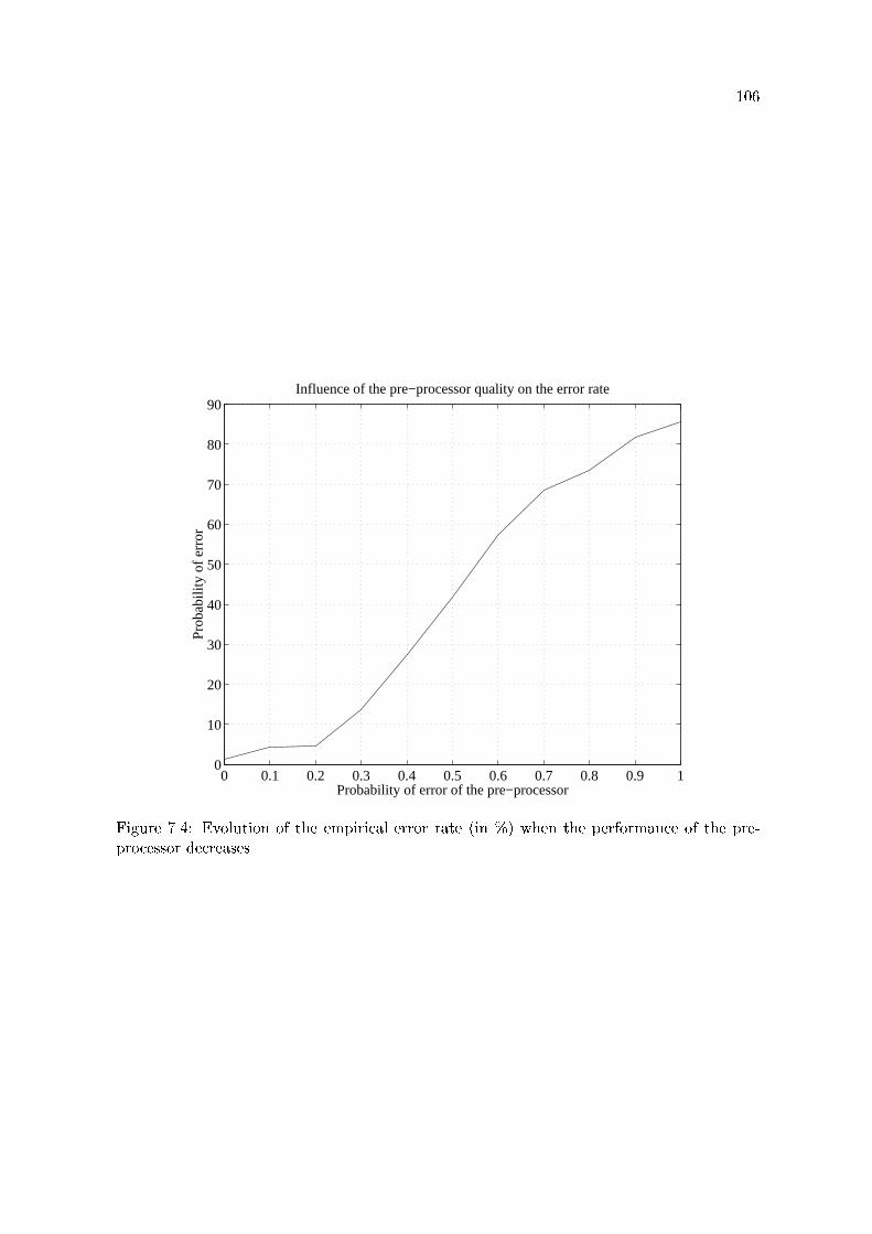
106
0 0.1 0.2 0.3 0.4 0.5 0.6 0.7 0.8 0.9 10
10
20
30
40
50
60
70
80
90
Probability of error of the pre−processor
Pro
babi
lity
of e
rror
Influence of the pre−processor quality on the error rate
Figure 7.4: Evolution of the empirical error rate (in %) when the performance of the pre-
processor decreases.

107
Chapter 8
Decomposition of Mixtures of
Continuous Hidden Markov Models
In the previous chapter, mixtures of discrete HMMs were applied to the classi�cation of
simultaneous signals. This application relied on the existence of a pre-processor mapping the
original continuous-time signal ~Y (t) onto a sequence of discrete symbols f ~Yng. It is likely
that some information is lost in the \discretization." In this chapter, we address the same
issue, but, here, we consider that the pre-processor provides continuous outputs. We start
by formulating the classi�cation of simultaneous signals in terms of the decomposition of a
mixture of continuous HMMs. Then, we discuss possible solutions.
8.1 Problem Formulation
The formulation of the classi�cation of multiple simultaneous signals as a mixture of
HMMs decomposition problem for continuous HMMs is similar to that for discrete HMMs.
The main di�erence is in the way the continuous output pre-processor used is modeled. Let
f ~Yng denote the output of the pre-processor when fed by the sum of simultaneous signals ~Y (t),
and let fYi;ng, i = 1; 2; : : : ; r, be the pre-processor output sequences that would be observed
if each of the component signals Yi(t) could be pre-processed separately. We assume that ~Yn
is a linear combination of the component processes Yi;n,
~Yn = q1Y1;n + q2Y2;n + � � �+ qrYr;n: (8.1)
where qi 2 R+0 . The coe�cients qi give the proportions of the di�erent components in f ~Yng.Expression (8.1) is a realistic model for the behavior of some types of pre-processors used
in signal processing or in environmental acoustics, for instance, a �lter bank followed by
short-time RMS integrators would correspond to this model. Further assume that each of
the processes fYi;ng can be a modeled by continuous HMM. Thus, f ~Yng is a mixture of
continuous hidden Markov models in the sense of Section 6.4.2.

108
HMM �cfyc;ng
qc
�
HMM �c�1fyc�1;ng
qc�1
�
.
.
.
HMM �2fy2;ng
q2
R
HMM �1fy1;ng
q1
U
�
-+ -
~yn =
Xi2�
qiyi;n
Figure 8.1: \Block" diagram for the decomposition of a mixture of continuous HMMs.
The classi�cation of multiple signals can now be expressed easily as a mixture decompo-
sition problem for MCHMMs. Let � = f�1; �2; : : : ; �cg be a dictionary of hidden Markov
models for the c possible component signals. The problem is: given a sample ~yN0 of f ~Yng,�nd the subset of indices � � f1; 2; : : : ; cg of the elements from � that are present in f ~Yng.Figure 8.1 summarizes the mixture model in a \block diagram" fashion. Decomposing the
mixture amounts to �nding the switches that are \on," all the \gains" qi beeing strictly
positive. Alternately, it can be assumed that all the switches are \on" but that some of the
\gains" are set equal to zero. Thus, the problem of �nding the components that are present
in f ~Yng can be formulated equivalently as �nding the switches that are \on" or as �nding
the components that have a non-zero \gain" qi.
Let Q = (q1; q2; : : : ; qc), qi 2 R+0 , be the set of coe�cients in the linear combination
(\gains"). If Q is known, the mixture decomposition problem is the exact analogous of that
of Chapter 7. The optimal solution will again be given by the Bayes decision rule. It will be
possible to compute to likelihoods using the forward-backward algorithm with the equivalent
HMMs given by the relations of Section 6.4.2. The same combinatorial optimization problem
will be encountered and the same sub-optimal solutions can be proposed, mutatis mutandis.
The case where Q is unknown is more di�cult, and also more interesting. It corresponds
to the situation where not only the component signals that are present in ~Y (t), but also their
proportions are unknown. This is a realistic assumption in many applications including noisy
speech recognition or environmental sound classi�cation (see the remark below). Possible
solutions are proposed for this case in the next section.
Remark 8.1 If all the processes are stationary and the dictionary of possible HMMs �

109
contains normalized models for the component processes fYi;ng, i.e.,
Var(Yi;n) = 1;
then we have
Var( ~Yn) =Xi2�
q2i ;
with � the set of indices corresponding to the true model. That is, q2i is the contribution
of the i-th signal to the total variance (power). This interpretation is particularly useful in
environmental acoustics since: it implies that estimating qi will provide a measure of the
contribution of the i-th sound source to the global sound level, information that is highly
desirable in noise control and noise monitoring.
8.2 Proposed Solutions
Denote by � = f�1; �2; : : : ; �cg the dictionary of possible components HMMs and by
� = f� : � � f1; 2; : : : ; cgg the set of all index sets for �. Let Q� = (q�1 ; q�2 ; : : : ; q�c),
qi 2 R+0 be the set of linear coe�cients associated with the index set �. Denote by ~��(Q�)
the parameter set of the continuous HMM equivalent to the MCHMM (��1 ; ��2 ; : : : ; ��r ;Q�).
The relation between ~��(Q�) = (A�;B� ;��) and ��i = (A�i ;B�i ;��i), i = 1; 2; : : : ; r, and
Q� is de�ned by (6.19),(6.21), and (6.31).
For a given subset of indices �, fp(~yN0 ; ~��(Q�)); Q� 2 (R+0 )rg de�nes a parametric familyof models for ~Y N
0 . Thus, given a length N + 1 sample ~yN0 , the selection of an index set �
for the components HMMs that are present in f ~Yng amounts to the choice of a parametric
family of models for f ~Yng. That is, the hypotheses for the test are
H� : ~Y N0 � p(~yN0 ; ~��(Q�)); for some Q� 2 (R+0 )r; 8� 2 �:
8.2.1 Penalized Likelihood Method
Since the parameters Q� associated with a hypothesis H� are not known, it seems in-
tuitively reasonable to try to estimate them under the hypothesis � and use the resulting
estimate in the decision statistic. If the MLE of Q� under H� is used, a decision rule is
� = argmax�2�
maxQ�2(R
+0 )
rp(~yN0 ;
~��(Q�)): (8.2)
The decision rule (8.2) is known as the maximum likelihood procedure (Lehmann 1986) or the
generalized likelihood ration test (GLRT) (Poor 1988). The GLRT is intuitively appealing
and often possesses good asymptotic properties (Lehmann 1986).
In our mixture decomposition problem, however, the GLRT fails completely for the fol-
lowing reason. Assume for a moment that qi can be equal to zero, and recall the analogy

110
between switches \o�" and null \gains" of Figure 8.1. Clearly, if �1 � �2, we have
maxQ�1
2(R+)r1p(~yN0 ;
~��1(Q�1)) � maxQ�2
2(R+)r1p(~yN0 ;
~��2(Q�1)):
If the likelihoods p(~yN0 ;~��(Q�)) are continuous on their boundary points, which is usually the
case, we also have
maxQ�1
2(R+0 )r1
p(~yN0 ;~��1(Q�1)) � max
Q�22(R+0 )
r1
p(~yN0 ;~��2(Q�1)):
It follows that � = f1; 2; : : : ; cg will always be a maximizer of (8.2), i.e., the likelihood ratio
procedure will always select all the components from the dictionary. This \over-�tting" is
very similar to what happens in model selection when nested families of models are used.
This naturally suggests the utilization of model selection methods to solve the problem. One
such model selection method is the penalized likelihood approach, which has already been used
in Section 5.2.9.2.
In the penalized likelihood approach, the decision rule is
� = !(~yN0 )
= argmin�2�
PL(�) (8.3)
The penalized likelihood criterion PL(�) used as a decision statistic in (8.3) is de�ned by
PL(�) = � maxQ�2(R
+0 )
rln p(~yN0 ;
~��(Q�)) + h(r;N + 1); (8.4)
where the penalty term is a function of the number of components r = #� (i.e., the number
of free parameters in the model) and of the sample length. Possible choices for the penalty
term h(k;N) leading to AIC or MDL selection criterion can be found in Section 5.2.9.2.
The evaluation of PL(�) requires a likelihood maximization. Even if an e�cient algorithm
for this maximization can be found (see below), this means that the computational cost of
the penalized likelihood approach will be high, especially since this maximization has to be
performed for all xi 2 �. The same combinatorial explosion as in the discrete case! If an
exhaustive exploration of � is not possible, sub-optimal search strategies can be employed in
(8.3). Another decision scheme is now proposed that can alleviate this problem.
8.2.2 �2 Test Method
Denote by �� be the \true" subset of indices and let �0; �1 2 � be two nested subsets of
indices, �0 � �1. Consider the composite hypotheses test
H0 : �� � �0
against the alternative
H1 : �� � �1; �� 6� �0:

111
Assuming that the �2 theory of maximum likelihood-ratio tests applies (Lehmann 1986,
Chapter 8), we would have asymptotically
2 lnt(�1)
t(�0)� �2r1�r0 ; (8.5)
where
t(�) = maxQ�2(R+)r
p(~yN0 ;~��(Q�))
and r0 = #�0, r1 = #�1. Note that using the \o� switch{null gain" analogy, the hypotheses
H0 and H1 can be reformulated as
H0 : qi = 0;8i 2 �1 n �0;H1 : 9i 2 �1 n �0 s.t. qi > 0:
The UMP decision rule for H0 against H1 at level � would be asymptotically equivalent to
the likelihood-ratio test
!(~yN0 ) =
8><>:O when t(�0) > k t(�1);
1 when t(�0) < k t(�1);
with the threshold k corresponding to � obtained from (8.5) for a �2 distribution with (r1�r0)degrees of freedom. We conjecture that the �2 theory of maximum likelihood-ratio test applies
to stationary ergodic continuous HMMs. Baum & Petrie (1966) proved that the �2 theory
of testing applied to stationary ergodic discrete HMMs, for the estimation of the parameters
�. We believe that it could be possible to extend the proofs to continuous HMMs, and more
particularly to the parameterization via linear coe�cients qi.
If the conjecture holds, we can propose the following algorithm for the continuous mixture
decomposition problem:
1. Initialization: let �1 = f1; 2; : : : ; cg.
2. Selection:
i� = argmaxi2�1
t(�1 n fig)
�0 = �1 n fi�g
3. If t(�0) > k t(�1), then �1 �0, goto 2.
4. Set � = �1.
The threshold k is obtained from a �21 distribution so as to insure a level � appropriately
chosen for the tests. The algorithm above can be viewed as an SBS selection scheme applied
to the dictionary � with a control of \depth" (number of components) by a �2 test. It will
require at mostc(c+1)
2 evaluations of the test statistic t(�).

112
8.2.3 Likelihood Maximization
Both methods that have been proposed, penalized likelihood and �2 likelihood-ratio tests,
require the computation of the test statistic
t(�) = maxQ�2(R+)r
p(~yN0 ;~��(Q�)):
Luckily, it will generally be possible to obtain an e�cient algorithm for this maximization.
The nature of the problem naturally suggests the utilization of an EM algorithm. For
notational simplicity, we will assume that � = f1; 2; : : : ; rg and will drop the � indexing
in the sequel. Denote by Q = (q1; q2; : : : ; qr) the parameter set over which the likelihood
p(~yN0 ;~�(Q)) is to be maximized, and by Q the maximizer:
Q = arg maxQ2(R+)r
p(~yN0 ;~�(Q)):
Let _Yi;n = qiYi;n, i = 1; 2; : : : ; r, and let _Yn = ( _Y1;n; _Y2;n; : : : ; _Yr;n). Note that we have
~Yn = _Y1;n + _Y2;n + � � � + _Yr;n:
We choose for the complete data ( _Y N0 ; ~XN
0 ). The auxiliary function is
Q( �Q;Q) = EQ[ln p( _YN0 ; ~XN
0 ; ~�( �Q)) j ~yN0 ]: (8.6)
where
ln p( _yN0 ; ~xN0 ;
~�(Q)) = ln ~�~x0 +NXn=1
ln ~a~xn�1~xn +NXn=0
ln _b~xn( _yn;�Q): (8.7)
with
_b~{( _yn; �Q) =rY`=1
1
q`b`;i`(
_y`;nq`
):
Substituting (8.7) in (8.6), we get
Q( �Q;Q) =NXn=0
X~{2 ~S
~ n(~{)rX`=1
(EQ
"ln b`;i`(
_Y`;n�q`
) j ~yN0 ; ~Xn = ~{
#� ln �q`
)+ �
=rX`=1
8<:
NXn=0
X~{2 ~S
~ n(~{)EQ
�ln b`;i`(
q`
�q`Y`;n) j ~yn; ~Xn = ~{
�� (N + 1) ln �q`
9=;+ �;
where ~ n(~{) = P [ ~Xn = ~{ j ~yN0 ] can be computed using a forward-backward recursion and
� is a term that does not depend on �Q. Given a current approximation Q of Q, the next
approximation �Q of Q is obtained by the EM iteration de�ned by
1. E-step: Determine Q( �Q;Q).
2. M-step: Choose �Q 2 arg max�Q2(R+0 )
rQ( �Q;Q).

113
The E and M steps reduce to the set of r decoupled re-estimation formulae:
�q` 2 arg max�q`2R
+0
8<:
NXn=0
X~{2 ~S
~ n(~{)EQ
�ln b`;i`(
q`
�q`Y`;n) j ~yn; ~Xn = ~{
�� (N + 1) ln �qi
9=; ;
(8.8)
for ` = 1; 2; : : : ; r. Note that if the HMMs have their state-conditional pdfs in the exponantial
family, the re-estimation formulae will become even simpler. For example, for a mixture of
Gaussian CHMMs, it is easy to see that EQhln b`;i`(
q`�q`Y`;n) j ~yn; ~Xn = ~{
ican be expressed as
a function of �q`, the conditional means EQ[Y`;n j ~yn; ~Xn = ~{] and the conditional covariances
CovQ(Y`;n j ~yn; ~Xn = ~{). The conditional means and conditional covariances are available in
closed form by (6.42) and (6.43), respectively. The maximizer �q` can be found analytically.

114
Chapter 9
Conclusion and Directions for
Future Research
In the �rst part of this work, the concept of hidden Markov model has been de�ned
in a mathematically rigorous fashion. Computational methods, inference procedures, and
applications have been reviewed. A special attention was dedicated to the classi�cation
problem. It appeared that Hidden Markov models form an interesting class of stochastic
processes with many useful applications.
In the second part of this work, the new concept of mixture of hidden Markov models has
been introduced. It was also shown how computational methods and inference procedures
originally developed for HMMs could be applied to mixtures of HMMs. Some original infer-
ence procedures were also proposed to address two issues speci�c to MHMMs: �ltering and
mixture decomposition. While the introduction of mixtures of HMMs was motivated by an
application in environmental sound recognition, it has been shown that they are of broader
interest. For instance, it has been shown how many \HMM extensions" previously developed
in speech processing or in radar/sonar/communication signal processing could be viewed as
special cases of our mixture of HMMs model.
The mixture decomposition problem has been the subject of more detailed attention in
the last two chapters. Algorithms were proposed to solve the mixture decomposition problem
for mixtures of discrete and continuous HMMs. However, the methods proposed leave open
a few questions and conjectures that are worthy of further theoretical work. Experimental
validation of the mixture decomposition paradigm for the classi�cation of simultaneous signals
should also be undertaken. Some alternative directions for future research will be discussed
now.
The Bayes rule (6.52) proposed for the decomposition of mixtures of discrete HMMs
assumed that the probabilistic observation mapping q was completely known. There are
situations in which it would be interesting either to consider a parametric form for q with
unknown parameters, or to allow some perturbation of the mapping q with respect to its

115
known model (a kind robust modeling). This would be a �rst area of research.
In Chapter 8, the mixture decomposition problem was stated for mixtures of continuous
HMMs with a deterministic observation mapping with unknown parameters. Two solutions
were proposed with a likelihood-based decision statistic (penalized likelihood or �2 test), but
some questions remain. For the penalized likelihood approach, the choice of penalty term
should be considered and the associated asymptotic properties of the decision rule should
be analyzed. We believe that the choice of the MDL penalty term should yield a consistent
decision rule (in the sense that the probability of error tends to zero when N increases).
For the �2 test method, the conjecture that the theory of likelihood-ration tests applies to
stationary ergodic HMMs should be veri�ed. The question of the identi�ability of a dictionary
of HMMs for the unknown parameter case also remains open. As an alternative to likelihood-
based methods, it would also be interesting to consider Bayesian methods. By including
additional a priori information in the form of a prior for the \gains" qi, Bayesian methods
could provide some improvements over likelihood methods, specially for small samples.
Finally, if mixture of HMMs decomposition is to be put to use in practical applications,
additional e�orts should be devoted to the research of computationally e�cient algorithms.
Methods that could lead to computational savings include approximations, alternative deci-
sion statistics, sub-optimal search strategies, and hybrid methods combining the three.
116
Appendix A
Discrete Markov Chains
The basic properties of discrete Markov chains are reviewed in this appendix. For more
details, see (Karlin & Taylor 1975, Ruegg 1989, Karr 1990).
A.1 De�nition
A discrete-time stochastic process fXn;n 2 Ng taking its values in a state space S is a
Markov chain if it possesses the Markov property:
P [Xn 2 AjXn�1; : : : ;X0] = P [Xn 2 AjXn�1]; 8n � 1; (A.1)
for all events A � S. If the state space S is discrete (�nite or countably in�nite), the Markov
chain is called a discrete Markov chain. The state space is frequently labeled by the positive
integers, or a subset thereof, and it is customary to speak of Xn being in state i if Xn = i.
A discrete Markov chain is completely de�ned by its set of one-step transition probabilities
a(n;n+1)ij = P [Xn+1 = jjXn = i]; (A.2)
and the initial distribution on the states
�(0)i = P [X0 = i]: (A.3)
A Markov chain is said to be homogeneous1 if the transition probabilities are independent
of n
a(n;n+1)ij = aij; 8n 2 N: (A.4)
Homogeneous Markov chains are the only one considered here.
1Or time homogeneous, if there is a need to emphasizes the temporal aspect, since there exists also Markov
chains that are spatially homogeneous (Karlin & Taylor 1975).

117
1 2
-a12
�a21
-a11 -
a22
Figure A.1: A two-state homogeneous Markov chain.
A.2 Properties of Markov Chains
A.2.1 Transition Probability Matrices of a Markov Chain
The set of transition probabilities is often represented by a transition probability matrix
A = (aij), or by a transition graph like that of Figure A.1 for a two-state chain with transition
probability matrix A = ( a11 a12a21 a22 ). Usually, a transition graph displays only the connections
between states corresponding to non-zero transition probabilities.
A transition probability matrix veri�es the properties:
1. aij � 0,
2.Xj
aij = 1.
A square matrix with these properties is termed a (row) stochastic matrix or aMarkov matrix.
Note that stochastic matrices are non-negative matrices, and the Perron-Frobenius theory of
non-negative matrices applies (Horn & Johnson 1985).
For a homogeneous Markov chain, the probability of an event fi0; i1; : : : ; ing is given by
P [Xn = in;Xn�1 = in�1; : : : ;X0 = i0] = �(0)i0
nYk=1
aik�1ik : (A.5)
Let a(n)ij denote the n-step transition probabilities
a(n)ij = P [Xn = jjX0 = i] (A.6)
= P [Xm+n = jjXm = i]; 8m � 0:
They obey the Chapman-Kolmogorov equations
Xk
a(m)ik a
(n)kj = a
(m+n)ij m � 1; n � 1; (A.7)
or, in matrix form,
A(m+n) = A(m)A(n); (A.8)

118
which implies
A(n) = An; (A.9)
where An denotes the n-th power of matrix A. Let �(n) =��(n)i
�be the row vector of state
probabilities �(n)i = P [Xn = i]. It can be shown that
�(n+1) = �(n)A; (A.10)
and
�(n) = �(0)An: (A.11)
A.2.2 Classi�cation of State of a Markov Chain
A state j is said to be accessible from i and the transition from i to j is possible, noted
j ! j, if there exists n � 0 such that a(n)ij > 0. If i ! j and j ! i, then i and j are said to
communicate, written i$ j. The communication relation$ is an equivalence relation, which
de�nes equivalence classes on the set of states S. A Markov chain is said to be irreducible if
there exists only one equivalence class, i.e., if all states communicate with each other.
The period of state i is the greatest common divisor (g.c.d.) of all n � 1 such that
a(n)ii > 0. A Markov chain in which each state has period one is called aperiodic. A state i is
absorbing if aii = 1.
Let Ti = infnfn � 1;Xn = ig. A state i is recurrent if P [Ti < 1jX0 = i] = 1. A state
that is not recurrent is called transient. It can be shown that if a state in an equivalence class
is recurrent, then all states in the class are recurrent, and the class is said to be recurrent. A
recurrent state i is null if E[Ti] =1; it is non-null or positive recurrent if E[Ti] <1.
Recurrence, transience and the period of a state are solidarity properties. That is, if C
is an equivalence class of states and i 2 C has the property, then every state j 2 C has the
property.
A Markov chain that is positive recurrent, aperiodic, and irreducible is is ergodic, and
conversely. Note that if the state space S is �nite, irreducibility and aperiodicity are su�cientconditions for ergodicity.
Example A.1 The �ve-state Markov chain of Figure A.2 with transition matrix
A =
0BBBBBBBB@
a11 a11 0 0 0
0 a22 a23 0 0
a31 a32 a33 0 0
0 0 0 a44 a45
0 a22 a11 0 1
1CCCCCCCCA

119
1
2
3 5
4
�
a12
Ia31
?a236a32 ?a45
-a22 -
a44
-a33
-a55
Figure A.2: An example of Markov chain.
is clearly not irreducible; it contains two positive recurrent classes: f1; 2; 3g and f5g. The
state 4 is transient. The state 1 is periodic with period 2; all other states are aperiodic. The
state 5 is absorbing.
A.2.3 Limit Behavior of a Markov Chain
A probability distribution �� is a stationary or stationary initial distribution if
�� = ��A: (A.12)
A Markov chain is stationary if the state distribution �(n) is independent of n, i.e., if �(0) is
a stationary initial distribution.
A Markov chain possess a limit distribution if
limn!1
�(n) = �� (A.13)
exists and is a probability distribution (Pi ��i = 1). The existence of the limit distribution
is guaranteed for ergodic Markov chains. Further more, it can be shown that if �� is the
limit distribution of an ergodic Markov chain, then �� = �� is its unique stationary initial
distribution.
The ergodic theorem for Markov chains states that, for an
limN!1
1
N + 1
NXn=0
f(Xn) =MXi=1
f(i)��i ; (A.14)
120
Appendix B
The EM Algorithm
The Expectation-Maximization (EM) algorithm has become one of the methods of choice
for maximum-likelihood (ML) estimation. In this appendix, based on the tutorial paper
(Couvreur 1996), the basic principles of the algorithm are described in an informal fashion
and illustrated on a notional example. Various applications to real-world problems are brie y
presented. We also provide selected entry points to the vast literature on the EM algorithm
for the reader interested in a rigorous mathematical treatment and further details on the
applications. We discuss the convergence properties of the algorithm and review some variants
and improvements that have been proposed. We conclude by some practical advice for the
practicing engineer interested in the implementation of the EM algorithm.
B.1 Introduction
Because of its asymptotic optimal properties, maximum-likelihood (ML) has become one
of the preferred methods of estimation in many areas of application of statistics, including
system identi�cation, speech and image processing, communication, computer tomography,
pattern recognition, and many others. Often, however, no theoretical solution of the likeli-
hood equations is available and it is necessary to resort to numerical optimization techniques.
Direct maximization of the likelihood function by standard numerical optimization methods
such as Newton-Raphson or gradient (scoring) methods is possible, but generally requires
heavy analytical preparatory work to obtain the gradient (and, possibly, the Hessian) of the
likelihood function. Moreover, the implementation of these methods may present numeri-
cal di�culties (memory requirements, convergence, instabilities, : : : ), particularly when the
number of parameters to be estimated is high (the dreaded \curse of dimensionality"). For
a certain class of statistical problems, an alternative to the direct numerical maximization
of the likelihood was introduced in 1977 by Dempster, Laird, and Rubin: the Expectation-
Maximization or EM algorithm (Dempster et al. 1977). The EM algorithm is a general
method for maximum-likelihood estimation for so-called \incomplete data" problems. Since

121
its inception it has been used successfully in a wide variety of applications ranging from
mixture density estimation to system identi�cation and from speech processing to computer
tomography.
The remainder of the appendix is organized as follows. In Section B.2, incomplete data
problems are de�ned and the EM algorithm for their solution is presented. A notional example
illustrates how the algorithm can be put to use. In Section B.3, arguments motivating
the choice of the EM algorithm for a ML problem are discussed and examples of practical
applications of the EM algorithm are brie y presented. The convergence properties of the
algorithm are the subject of Section B.4. Some variants of the EM algorithm are reviewed
in Section B.5. We conclude by a summary of the advantages and disadvantages of the EM
algorithms when compared to other likelihood maximization methods.
B.2 The EM Algorithm
B.2.1 Incomplete Data Problems
Let X and Y be two sample spaces, and let H be a many-to-one transformation from Xto Y. Let us assume that the observed random variable y in Y is related to an unobserved
random variable x by y = H(x). That is, there is some \complete" data x which is only
partially observed in the form of the \incomplete data" y. Let p(xj�) be the parametric
distribution of x, where � is a vector of parameters taking its values in �. The distribution
of y, denoted by q(yj�), is also parameterized by � since
q(yj�) =ZH(x)=y
p(xj�)dx: (B.1)
Estimation of � from y is an incomplete data problem. For example, an incomplete data
problem arises in signal processing when parameters have to be estimated from a coarsely
quantized signal: the complete data are the analog values of the signal (non-measured), the
incomplete data are the values of the signal quantized on a few bits. Other typical examples
of incomplete data problems can be found, e.g., in (Dempster et al. 1977).
B.2.2 The EM Algorithm
The maximum-likelihood estimator � is the maximizer of the log-likelihood
L(�) = ln q(yj�) (B.2)
over �, i.e.,
� = argmax�2�
L(�): (B.3)
The main idea behind the EM algorithm is that, in some problems, the estimation of � would
be easy if the complete data x was available while it is di�cult based on the incomplete data
122
y only (i.e., the maximization of ln p(xj�) over � is easily performed while the maximization
of ln q(yj�) is complex). Since only the incomplete data y is available in practice, it is not
possible to perform directly the optimization of the complete data likelihood ln p(xj�). In-
stead, it seems intuitively reasonable to \estimate" log p(xj�) from y and use this \estimated"
likelihood function to obtain the maximizer �. Since estimating the complete data likelihood
ln p(xj�) requires �, it is necessary to use an iterative approach: �rst estimate the complete
data likelihood given the current value of �, then maximize this likelihood function over �,
and iterate, hoping for convergence. The \best estimate" of log p(xj�) given a current value
�0 of the parameters and y is the conditional expectation
Q(�; �0) = E[log p(xj�)jy; �0]: (B.4)
Following this heuristic argument, the E and M steps of the iterative EM algorithm (also
known as the Generalized EM algorithm or GEM) can be formally expressed as:
E-step: compute
Q(�; �(p)) = E[log p(xj�)jy; �(p)]; (B.5)
M-step: choose
�(p+1) 2 argmax�2�
Q(�; �(p)): (B.6)
where �(p) denotes the value of the parameter obtained at the p-th iteration. Note that,
if the complete data distribution belong to the exponential (Koopmans-Darmois) family, the
algorithm takes a slightly simpler form (Dempster et al. 1977). The EM algorithm will be
now illustrated on a notional example.
B.2.3 A Notional Example
Let y = (y1; y2; : : : ; yN ) be a sequence of i.i.d. observations drawn from a mixture of two
univariate Gaussians with means �1 and �2, variances �21 and �
22, and mixing proportions �1
and �2. That is, yk � q(y) where
q(y) = �1q1(y) + �2q2(y); y 2 RI (B.7)
with �1 + �2 = 1 and
qj(y) =1p2��i
exp�12
�y � �j�
�2; j = 1; 2:
For simplicity, assume that the variances and mixing proportions are known. The unknown
parameters that have to be estimated from y�are the means, i.e., � = f�1; �2g. The log-
likelihood of � is given by
ln q(yj�) =NXk=1
ln q(ykj�): (B.8)

123
The maximization of (B.8) can be easily performed by casting the mixture problem as an
incomplete data problem and by using the EM algorithm. Drawing a sample y of a random
variable with mixture pdf (B.7) can be interpreted as a two step process. First, a Bernoulli
random variable i taking value 1 with probability �1 or value 2 with probability �2 = 1� �1is drawn. According to the value of i, y is then drawn from one of the two populations
with pdf q1(y) and q2(y). Of course, the \selector" variable i is not directly observed. The
complete data is thus x = (x1; x2; : : : ; xN ) with xk = (yk; ik), and the associated complete
data log-likelihood is
ln p(xj�) =NXk=1
ln p((yk; ik)j�)
with
p(xkj�) = �ikqik(yk)
= �1q1(yk)1fik=1g + �2q2(yk)1fik=2g;
where 1A is the indicator function for the event A. The auxiliary function is then easily seen
to be equal to
Q(�; �0) = E[ln p(xj�)jy; �0]
=NXk=1
2Xj=1
[ln�j + ln qj(yk)]P [ik = jjy; �0]:
From (B.9) it is straightforward to show that the EM algorithm (B.5){(B.6) reduces to a pair
of re-estimation formulae for the means of the mixture of two Gaussians:
�(p+1)1 =
1
N
NXk=1
ykP [ik = 1jyk; �(p)] (B.9)
�(p+1)2 =
1
N
NXk=1
ykP [ik = 2jyk; �(p)] (B.10)
where the a posteriori probabilities P [ik = jjyk; �(p)], j = 1; 2, can be obtained by the Bayes
rule
P [ik = jjyk; �(p)] =�jqj(ykj�(p))P2j=1 �jqj(ykj�(p))
: (B.11)
These re-estimation formulae have a satisfying intuitive interpretation. If the complete
data was observable, the ML estimators for the means of the mixture components would be
�j =1
N
NXk=1
yk1fik=jg; j = 1; 2: (B.12)
That is, each of the observations yk is classi�ed as coming from the �rst or the second
component distributions and the means are computed by averaging the classi�ed observations.

124
With only the incomplete data, the observations are still \classi�ed" in some sense: at each
iteration, they are assigned to both the �rst and the second component distributions with
weights depending on the posterior probabilities given the current estimate of the means.
The new estimates of the means are then computed by a weighted average.
B.3 Practical Applications
B.3.1 Motivation
The EM algorithm is mainly used in incomplete data problems when the direct maxi-
mization of the incomplete data likelihood is either not desirable or not possible. This can
happen for various reasons. First, the incomplete data distribution q(yj�) may not be easily
available while the form of the complete data distribution p(xj�) is known. Of course, rela-tion (B.1) could be used, but the integral may not necessarily exist in closed form and its
numerical computation may not be possible at a reasonable cost, especially in high dimen-
sion. Next, even if a closed form expression for q(yj�) is available, the implementation of
a Gauss-Newton, scoring, or other direct maximization algorithm might be di�cult because
it requires a heavy preliminary analytical work in order to obtain the required derivatives
(gradient or Hessian) of q(yj�) or because it requires too much programming work. The EM
algorithm, on the other hand, can often be reduced to a very simple re-estimation procedure
without much analytical work (like in the notional example of the previous section). Finally,
in some problems, the high dimensionality of � can lead to memory requirements for direct
optimization algorithms exceeding the possibilities of the current generation of computers.
The PET tomography application below is an example of how the EM algorithm can some-
times provide a solution requiring little storage in this case. There are other arguments in
favor of the utilization of the EM algorithm; there are also some drawbacks. They will be
discussed in the last sections.
To give the reader a avor of the kind of ML problems in which the EM algorithm
is currently used, we now brie y review some applications. It will be seen that the EM
algorithm leads to an elegant and heuristically appealing formulation in many cases. The
applications will be simply outlined and the interested reader will be referred to the literature
for further details. As much as possible, we tried to provide references to the key papers in
each �eld rather than attempting to give an exhaustive bibliographic review (which would
have been outside of the scope of this paper anyway). We also tried to provide examples that
are of interest for the control and signal processing community.

125
B.3.2 Examples of Applications
B.3.2.1 Mixture Densities
A family of �nite mixture densities is of the form
q(yj�) =KXj=1
�jqj(yj�j); y 2 RI d (B.13)
where �j � 0,PKj=1 �j = 1, qj(yj�j) is itself a density parameterized by �j , and � =
f�1; : : : ; �K ; �1; : : : ; �Kg. The complete data is naturally formulated as the combination
of the observations y with multinomial random variables i acting as \selectors" for the com-
ponent densities qj(yj�i), like in the notional example. Let y = (y1; y2; : : : ; yN ) be a sample
of i.i.d. observation, yk � q(ykj�). It can be shown (Redner & Walker 1984) that the EM
algorithm for the ML estimation of � reduces to the set of re-estimation formulae
�(p+1)j =
1
N
NXk=1
�(p+1)j qj(ykj�(p)j )
q(ykj�(p));
�(p+1)j 2 argmax
�j
NXk=1
�ln qj(ykj�j)�
�(p+1)j qj(ykj�(p)j )
q(ykj�(p))
#;
for j = 1; : : : ;K. Again, the solution has a heuristically appealing interpretation as a
weighted ML solution. The weight associated with yk is the posterior probability that the
sample originated from the jth distribution, i.e., the posterior probability that the selector
variable ik is equal to j. Furthermore, in most applications of interest �(p+1) is uniquely and
easily determined from (B.14), like in the mixture of two Gaussians presented in the notional
example of Section B.2.3.
The EM algorithm for mixture densities is widely used in statistics and signal processing,
for example, for clustering or for vector quantization with a mixture of multivariate Gaussians.
Moreover, the well-known Baum-Welsh algorithm used for the training of hidden Markov
models in speech recognition (Rabiner 1989) is also an instance of the EM algorithm for
mixtures with a particular Markov distribution for the \selectors" ik (Titterington 1990).
B.3.2.2 PET Tomography
The EM algorithm has been used for over a decade to compute ML estimate of radionu-
cleide distributions from tomographic data, such as that measured by positron emission
tomography (PET) (Shepp & Vardi 1982, Vardi, Shepp & Kaufman 1985). It relies on the
following statistical model. Assume that the radionucleide distribution discretized into d
pixels with emission rates � = (�1; : : : ; �d). Assume that there are N detectors and let xnk
denote the number of emissions from the kth pixel that are detected by the nth detector.
The variates xnk are assumed to have independent Poisson distribution:
xnk � Poisson with rate ank�k;

126
where the ank are non-negative (known) constants that characterize the measurement system.
Neglecting background emissions, random coincidences, and scatter contamination, the total
number of detections at the nth sensor is yn =Pdk=1 xnk. The ML estimate of � can be
obtained by applying the EM algorithm to the complete data x = (xnk), 1 � n � N ,
1 � k � d, with the incomplete data y = (y1; : : : ; yN ). It can be shown that the EM algorithm
reduces to re-estimation formulae which are extremely simple and easy to implement (Vardi
et al. 1985). Many variations of the EM algorithm have been proposed for PET image
reconstruction, e.g., (Fessler & Hero 1994, Silverman, Jones, Wilson & Nychka 1990).
B.3.2.3 System Identi�cation
Consider the discrete-time linear stochastic system with state and observation equations
xt+1 = Fxt + ut
yt = Hxt + vt
where ut and vt are Gaussian zero-mean vector random processes with covariance matrices
�u and �v, respectively, and F and H are matrices of appropriate dimensions. Let y =
(y1; y2; : : : ; yN ) be a length N sample of the output of the system, and let � = fF;H;�u;�vgbe the parameter set of interest. The estimation of � from y lends itself naturally to a
formulation as an incomplete data problem and the EM algorithm can be used to compute
�. In this case, the complete data is simply the combination of the state and observation
vectors, i.e., x = ((x1; y1); : : : ; (xN ; yN )). The E-step can be handled by a Kalman smoother,
and the M-step reduces to a linear system of equations with a closed form solution (Shumway
& Sto�er 1982) (see also (Segal & Weinstein 1988) and (Segal & Weinstein 1989)). This EM
approach to ML system identi�cation can be straightforwardly extended to deal with missing
observations (Shumway & Sto�er 1982, Digalakis, Rohlicek & Ostendorf 1993) or coarsely
quantized observations (Ziskand & Hertz 1993).
B.4 Convergence Properties
It is possible to prove some general convergence properties of EM algorithms. Since the
EM algorithm is a \meta-algorithm," a method for implementing ML algorithms, the results
are universal in the sense that they apply to the maximization of a wide class of incomplete
data likelihood functions.
B.4.1 Monotonous Increase of the Likelihood
The sequence f�(p)g generated by the EM algorithm increases monotonously the likelihood
L(�); that is,
L(�(p+1)) � L(�(p)):

127
This property is a direct corollary of the next theorem.
Theorem B.1 If
Q(�; �0) � Q(�0; �0)then
L(�) � L(�0):
Proof. Let r(xjy; �) denote the conditional distribution of x given y, r(xjy; �) = p(xj�)=q(yj�),and let
V (�; �0) = E[ln r(xjy�; �)jy; �0]:
From (B.2), (B.4), and this de�nition, we have
L(�) = Q(�; �0)� V (�; �0):Invoking Jensen's inequality, we get
V (�; �0) � V (�0; �0);and the theorem follows. �
Corollary B.1 Let f�(p)g denote a sequence of estimate of � generated by the EM algo-
rithm. We have
L(�(p+1)) � L(�(p)); 8p � 0:
B.4.2 Convergence to a Local Maxima
The global maximization of the auxiliary function performed during the M-step can be
misleading. With the exception of a few speci�c cases, the EM algorithm is not guaranteed
to converge to a global maximizer of the likelihood. Under some regularity conditions on
the likelihood L(�) and on the parameters set �, it is possible, however, to show that the
sequence f�(p)g obtained by EM algorithm converges to a local maximizer of L(�), or, at
least, to a stationary point of L(�). Necessary conditions for the convergence of the EM
algorithm and related theorems can be found in (Wu 1983). Note that the original proof
of convergence of the EM algorithm given in (Dempster et al. 1977) was incorrect (see the
counter-example of Boyles (Boyles 1983)). Convergence results are also available for various
particular applications of the EM algorithm, e.g., in (Redner & Walker 1984) for mixtures of
densities.
Remark B.1 The reader should not confuse the algorithmic convergence of the EM algo-
rithm towards a local maximizer of the likelihood function for given data with the stochastic
convergence of the likelihood estimate towards the true parameters when the amount of
observed data increases (i.e., the consistency of the maximum likelihood estimator).

128
B.4.3 Speed of Convergence
It can be shown that, near the solution, the EM algorithm converges linearly. The rate of
convergence corresponds to the fraction of the variance of the complete data score function
unexplained by the incomplete data (Dempster et al. 1977, Louis 1982) (see also (Meng &
Rubin 1994)). That is, if the complete data model is much more informative about � than
the incomplete data model, then the EM algorithm will converge slowly.
B.5 Variants of the EM Algorithm
B.5.1 Acceleration of the Algorithm
In practice, the convergence of the EM algorithm can be desperately slow in some case.
Roughly speaking, the EM algorithm is the equivalent of a gradient method whose linear
convergence is well known. Variants of the EM algorithms with improved convergence speed
have been proposed. They are usually based on the application to the EM algorithm of
optimization theory techniques such as conjugate gradient (Jamshidian & Jennrich 1993),
Aitkin's acceleration (Meilijson 1989), or coordinate ascent (Fessler & Hero 1994, Segal &
Weinstein 1988). Many acceleration schemes have also been proposed for speci�c EM appli-
cations.
B.5.2 Approximation of the E or M Step
Another cause of slowness of the EM algorithm arises when the E or M step does not admit
an analytical solution. It becomes then necessary to use iterative methods for the computation
of the expectation or for the maximization, which can be computationally expensive. Variants
of the EM algorithm preserving its convergence properties have been proposed that can
alleviate this problem, e.g., (Celeux & Diebolt 1990, Cardoso, Lavielle & Moulines 1995, Meng
& Rubin 1993, Lange 1995). They are based on approximations of the E or M steps that
preserve the convergence properties of the algorithm. For example, it is shown in (Celeux &
Diebolt 1990) and (Celeux & Diebolt 1986) that the algorithm still converges if a Monte-Carlo
approximation of the E step is used. Furthermore, this approximation can even decrease the
probability of getting stuck in a local maxima.
B.5.3 Penalized Likelihood Estimation
The EM algorithm can be straightforwardly modi�ed to compute penalized likelihood
estimates (Dempster et al. 1977), that is, estimates of the form
~� = argmax�2�
[L(�) +G(�)] :
The penalty term G(�) could represent, for example, the logarithm of a prior on � if a Bayesian
approach is used and the maximum a posteriori (MAP) estimate of � is desired instead of
129
the ML estimate. The EM algorithm for penalized-likelihood estimation can be obtained by
replacing the M-step with (Dempster et al. 1977)
�(p+1) = argmax�2�
hQ(�; �(p)) +G(�)
i:
It is straightforward to see that the monotonicity property of Section B.4.1 is preserved, i.e.,
L(�(p+1)) +G(�(p+1)) � L(�(p)) +G(�(p)). Some extensions of the EM algorithm for dealing
speci�cally with penalized likelihood problems have been proposed, e.g., in (Green 1990) and
(Segal, Bacchetti & Jewell 1994). It is also noted in (Green 1990) that the inclusion of a
penalty term can speed up the convergence of the EM algorithm.
B.6 Concluding Remarks
As with all numerical methods, the EM algorithm should not be used with uncritical faith.
In fact, given an identi�cation/estimation problem the engineer should �rst ask whether
maximum likelihood is a good method for the speci�c application, and only then if the EM
algorithm is a good method for the maximization of the likelihood. The alternatives to
the EM algorithm include the scoring and Newton-Raphson methods that are commonly
used in statistics and any other numerical maximization method that can be applied to
the likelihood function. When is the EM algorithm a reasonable approach to a maximum-
likelihood problem? Compared to its rivals, the EM algorithm possesses a series of advantages
and disadvantages. The decision to use the EM algorithm should be based on an analysis of
the trade-o�s between those.
The main advantages of the EM algorithm are its simplicity and ease of implementation.
Unlike, say, the Newton-Raphson method, implementing the EM algorithm does not usually
require heavy preparatory analytical work. It is easy to program: either it reduces to very
simple re-estimation formulae or it is possible to use standard code to perform the E step
(like the Kalman smoother in the examples of Section B.3.2.3). Because of its simplicity, it
can often be easily parallelized and its memory requirements tend to be modest compared to
other methods. Also, the EM algorithm is numerically very stable. In addition, it can often
provide �tted values for the complete data without the need of further computation (they
are obtained during the E step).
The main disadvantage of the EM algorithm is its hopelessly slow linear convergence
is some case. Of course, the acceleration schemes of Section B.5.1 can be used, but they
generally require some preparatory analytical work and they increase the complexity of the
implementation. Thus, the simplicity advantages over other alternative methods may be lost.
Furthermore, unlike other methods based on the computation of derivatives of the incomplete
data log-likelihood, the EM algorithm does not provide an estimate of the information matrix
of � as a by-product, which can be a drawback when these estimates are desired. Extensions
of the EM algorithm have been proposed for that purpose though ((Meng & Rubin 1991) and

130
references therein, or (Louis 1982, Meilijson 1989)), but, again, they increase the complexity
of the implementation.
Finally, a word of advice for the practicing engineer interested in implementing the EM
algorithm. The EM algorithm requires an initial estimate of �. Since multiple local maxima
of the likelihood function are frequent in practice and the algorithm converges only to a local
maxima, the quality of the initial estimate can greatly in uence the �nal result. The initial
estimate should be carefully chosen. As with all numerical optimization methods, it is often
sound to try various initial starting points. Also, because of the slowness of convergence of
the EM algorithm, the stopping criterion should be selected with care.
In conclusion, the EM algorithm is a simple and versatile procedure for likelihood max-
imization in incomplete data problems. It is elegant, easy to implement, numerically very
stable, and its memory requirements are generally reasonable, even in very large problems.
However, it also su�ers from several drawbacks, the main one being its hopelessly slow con-
vergence in some cases. Nevertheless, we believe that the EM algorithm should be part of the
\numerical toolbox" of any engineer dealing with maximum likelihood estimation problems.

131
Bibliography
Akaike, H. (1974), `A new look at the statistical model identi�cation', IEEE Transactions on
Automatic Control 19(6), 716{723.
Albert, P. S. (1991), `A two-state hidden Markov mixture model for a time series of epileptic
seizure counts', Biometrics 47, 1371{1381.
Anderson, J. S. & Bratos-Anderson, M. (1993), Noise: its Measurement, Analysis, Rating
and Control, Aldershot: Aveburry Technical.
Anderson, T. W. (1984), An Introduction to Multivariate Statistical Analysis, second edn,
John Wiley & Sons, New York.
Ant�on-Haro, C., Fonollosa, J. A. R. & Fonollossa, J. R. (1996), On the inclusion of channel's
time dependence in a hidden Markov model for blind channel estimation, in `Proceedings
8th IEEE Signal Processing Workshop on Statistical Signal and Array Processing', IEEE
Computer Society Press, Corfu, Greece, pp. 164{167.
Askar, M. & Derin, H. (1981), `A recursive algorithm for the Bayes solution of the smoothing
problem', IEEE Transactions on Automatic Control 26(2), 558{561.
Ayanoglu, E. (1992), `Robust and fast failure detection and prediction for fault-tolerant
communication network', Electronics Letters 28(10), 940{941.
Bahl, L. R., Jelinek, F. & Mercer, R. L. (1983), `A maximum likelihood approach to contin-
uous speech recognition', IEEE Transactions on Pattern Analysis and Machine Intelli-
gence 5(2), 179{190.
Baker, J. K. (1975), `The DRAGON system|an overview', IEEE Transactions on Acoustics,
Speech and Signal Processing 23(1), 24{29.
Baldi, P. & Chauvin, Y. (1994), `Smooth on-line learning algorithms for hidden Markov
models', Neural Computations 6(2), 307{318.
Baum, L. E. (1972), `An inequality and associated maximization techniques in statistical
estimation for probabilistic functions of Markov processes', Inequalities 3, 1{8.

132
Baum, L. E., Petrie, T., Soules, G. & Weiss, N. (1970), `A maximization technique occur-
ing in the statistical analysis of probabilistic functions of Markov chains', Annals of
Mathematical Statistics 41(1), 164{171.
Baum, L. E. & Sell, G. H. (1968), `Growth functions for functions on manifolds', Paci�c
Journal of Mathematics 27(2), 211{227.
Baum, L. & Eagon, J. A. (1967), `An inequality with applications to statistical estimation
for probabilistic functions of Markov processes and to a model for ecology', Bulletin of
the American Mathematical Society 73, 360{363.
Baum, L. & Petrie, T. (1966), `Statistical inference for probabilistic functions of �nite state
Markov chains', Annals of Mathematical Statistics 37, 1554{1563.
Besag, J. E. (1986), `On the statistical analysis of dirty pictures (with discussion)', Journal
of the Royal Statistical Society B 48, 192{236.
Bickel, P. J. & Rytov, Y. (1994), Inference in hidden Markov models I: Local asymptotic nor-
mality in the stationary case, Technical Report 383, Department of Statistics, University
of California, Berkeley.
Bourlard, H., Konig, Y. & Morgan, N. (1994), REMAP: recursive estimation and maximiza-
tion of a posteriori probabilities, application to transition-based connectionist speech
recognition, Technical Report TR-94-064, International Computer Science Institute
(ICSI), Berkeley California.
Bourlard, H. & Wellekens, C. (1990), `Links between Markov models and multilayer percep-
trons', IEEE Transactions on Pattern Analysis and Machine Intelligence 12(12), 1167{
1179.
Boyles, R. A. (1983), `On the convergence of the EM algorithm', Journal of the Royal Sta-
tistical Society B 45(1), 47{50.
Bridle, J. S. (1990), `Alpha-nets: A recurrent \neural" network architecture with a hidden
Markov model interpretation', Speech Communication 9, 83{92.
Burshtein, D. (1995), Robust parametric modeling of durations in hidden Markov models, in
`Proceedings of the International Conference on Acoustics, Speech and Signal Process-
ing', IEEE, Detroit, pp. 548{551.
Cardoso, J.-F., Lavielle, M. & Moulines, E. (1995), `Un algorithme d'identi�cation par max-
imum de vraisemblance pour des donn�es incompl�etes', Comptes Rendus de l'Acad�emie
des Sciences de Paris, S�erie I 320, 363{368. in French.

133
Celeux, G. & Diebolt, J. (1986), `L'algorithme SEM : un algorithme d'apprentissage proba-
biliste pour la reconnaissance de m�elanges de densit�es', Revue de Statistiques Appliqu�ees
24(2), 35{52.
Celeux, G. & Diebolt, J. (1990), `Une version de type recuit simul�e de l'algorithme EM',
Comptes-Rendu de l'Acad�emie des Sciences de Paris, S�erie I 310, 119{124.
Chen, J. L. & Kundu, A. (1994), `Rotation and gray scale transform invariant texture iden-
ti�cation using wavelet decomposition and hidden Markov models', IEEE Transactions
on Pattern Analysis and Machine Intelligence 16(2), 208{214.
Coast, Stern, Cano & Briller (1990), `An approach to cardiac arythmia analysis using hidden
Markov models', IEEE Transactions on Biomedical Engineering 37(9), 826{836.
Collings, I. B., Krishnamurthy, V. & Moore, J. B. (1994), `On-line identi�cation of hidden
Markov models via recursive prediction error techniques', IEEE Transactions on Signal
Processing 42(12), 3535{3539.
Couvreur, C. (1995), Estimation of parameters and classi�cation of mixtures of autoregressive
processes, Master's thesis, University of Illinois at Urbana-Champaign.
Couvreur, C. (1996), The EM algorithm: A guided tour, in `Proc. 2nd IEEE European
Workshop on Computer-Intensive Methods in Control and Signal Processing', Pragues,
Czech Rep.
Couvreur, C. & Bresler, Y. (1995a), Decomposition of a mixture of Gaussian AR processes,
in `Proceedings IEEE International Conference on Acoustic, Speech, and Signal Pro-
cessing', Detroit, MI, pp. 1605{1608.
Couvreur, C. & Bresler, Y. (1995b), A statistical pattern recognition framework for noise
recognition in an intelligent noise monitoring system, in `Proceedings EURO-NOISE '95',
Lyon, France, pp. 1007{1012.
Couvreur, C. & Bresler, Y. (1996), Dictionary-based decomposition of linear mixtures of
Gaussian processes, in `Proceedings IEEE International Conference on Acoustic, Speech,
and Signal Processing', Atlanta, GA. To appear.
Couvreur, C., Fontaine, V. & Leich, H. (1996), Discrete HMM's for mixtures of signals, in
`Proceedings VIII European Signal Processing Conference', Trieste, Italy. To appear.
Cox, D. R. (1990), `Role of models in statistical analysis', Statistical Science 5(2), 169{174.
Csisz�ar, I. & Narayan, P. (1988), `Arbitrarily varying channels with constrained inputs and
states', IEEE Transactions on Information Theory 34(1), 27{34.

134
Dai, J. (1994), `Hybrid approach to speech recognition using hidden Markov models and
Markov chains', IEE Proceedings, Vision, Image, and Signal Processing 141(5), 273{
279.
Delyon, B. (1995), `Remarks on linear and nonlinear �ltering', IEEE Transactions on Infor-
mation Theory 41(1), 317{322.
Dempster, A. P., Laird, N. M. & Rubin, D. B. (1977), `Maximum likelihood from incomplete
data via the EM algorithm', Journal of the Royal Statistical Society B 39, 1{38.
Devijver, P. A. (1985), `Baum's forward-backwards algorithm revisited', Pattern Recognition
Letters 1, 369{373.
Devijver, P. R. & Kittler, J. (1982), Pattern Recognition: A Statistical Approach, Prentice-
Hall, Englewood-Cli�s, N.J.
Dey, S., Krishnamurthy, V. & Salmon-Legagneur, T. (1994), `Estimation of Markov-
modulated times-series via EM algorithm', IEEE Signal Processing Letters 1(10), 153{
155.
Digalakis, V., Rohlicek, J. R. & Ostendorf, M. (1993), `ML estimation of a stochastic lin-
ear system with the EM algorithm and its application to speech recognition', IEEE
Transactions on Speech and Audio Processing 1(4), 431{442.
Digalakis, V. V., Rtischev, D. & Neumeyer, L. G. (1995), `Speaker adaptation using con-
strained estimation of Gaussian mixtures', IEEE Transaction on Speech and Audio Pro-
cessing 3(5), 357{366.
Duda, R. O. & Hart, P. E. (1973), Pattern Classi�cation and Scene Analysis, John Willey &
Son, New-York.
Dugast, C., Beyerlein, P. & Haeb-Umbach, R. (1995), Application of clustering techniques
to mixture density moldeling for continuous speech recognition, in `Proceedings of the
International Conference on Acoustics, Speech and Signal Processing', IEEE, Detroit,
pp. 524{527.
Elliot, R. J., Aggoun, L. & Moore, J. B. (1995), Hidden Markov Models: Estimation and
Control, Springer-Verlag, New York.
Ephraim, Y. (1992a), `A Bayesian estimation approach for speech enhancement using hidden
Markov models', IEEE Transactions on Signal Processing 40(4), 725{735.
Ephraim, Y. (1992b), `Gain-adapted hidden Markov models for speech recognition of clean
and noisy speech', IEEE Transactions on Signal Processing 40(6), 1303{1316.
135
Ephraim, Y. (1992c), `Statistical-model-based speech enhancement systems', Proceedings of
the IEEE 80(10), 1526{1555.
Ephraim, Y., Dembo, A. & Rabiner, L. R. (1989), `A minimum discrimination informa-
tion approach for hidden Markov modeling', IEEE Transactions on Information Theory
35(5), 1001{1013.
Ephraim, Y. & Rabiner, L. R. (1990), `On the relations between modeling approaches for
speech recognition', IEEE Transactions on Information Theory 36(2), 372{380.
Fessler, J. A. & Hero, A. O. (1994), `Space-alternating generalized expectation-maximization
algorithm', IEEE Transactions on Signal Processing 42(10), 2664{2677.
Fielding, K. H. & Ruck, D. W. (1995), `Spatio-temporal pattern recognition using hidden
Markov models', IEEE Transactions on Aerospace and Electronic Systems 31(4), 1292{
1300.
Forney, G. D. (1973), `The Viterbi algorithm', Proceedings of the IEEE 61(3), 268{278.
Franco, H. & Serralheiro, A. (1991), Training HMMs using a minimum recognition error
approach, in `Proceedings of the International Conference on Acoustics, Speech and
Signal Processing', IEEE, Toronto, pp. 357{360.
Francq, C. & Roussignol, M. (1995), On white noises driven by hidden Markov chains, Techni-
cal Report 28, �Equipe d'Analyse et de Math�ematiques Appliqu�ees, Universit�e de Marne-
la-Vall�ee, France.
Frasconi, P. & Bengio, Y. (1994), An EM approach to grammatical inference: Input/output
HMMs, in `Proceedings of the 12th IAPR International Conference on Pattern Recog-
nition', IEEE Computer Society Press, Jerusalem, pp. 289{294.
Fredkin, D. R. & Rice, J. A. (1992), `Bayesian restoration of single-channel patch clamp
recordings', Biometrics 48, 428{448.
Frenkel, L. & Feder, M. (1995), Recursive estimate-maximize (EM) algorithms for time vary-
ing parameters with applications to multiple target tracking, in `Proceedings of the
International Conference on Acoustics, Speech and Signal Processing', IEEE, Detroit,
pp. 2068{2071.
Fwu, J. & Djuric, P. M. (1996), Automatic segmentation of piecewise constant signals by
hidden Markov models, in `Proceedings 8th IEEE Signal Processing Workshop on Sta-
tistical Signal and Array Processing', IEEE Computer Society Press, Corfu, Greece,
pp. 283{286.
136
Gales, M. J. F. & Young, S. J. (1992), An improved approach to the hidden Markov model
decomposition of speech and noise, in `Proceedings of the International Conference on
Acoustics, Speech and Signal Processing', IEEE, San Fransisco, CA, pp. I{233{I{236.
Gales, M. J. F. & Young, S. J. (1993a), HMM recognition in noise using parallel model
combination, in `Proceedings Eurospeech', Berlin, pp. 837{840.
Gales, M. J. F. & Young, S. J. (1993b), Parallel model combination for speech recognition in
noise, Technical Report CUED/F-INFENG/TR 135, Cambridge University, Cambridge,
England.
Gauvain, J. & Lee, C. (1994), `Maximum a posteriori estimation for multivariate Gaussian
mixture observations of Markov chains', IEEE Transactions on Speech and Audio Pro-
cessing 2, 291{298.
Gelb, A. (1974), Applied Optimal Estimation, M.I.T. Press, Cambridge, MA.
Geman, S. & Geman, D. (1984), `Stochastic relaxation, Gibbs distribution, and the Bayesian
restoration of images', IEEE Transactions on Pattern Analysis and Machine Intelligence
6(6), 721{741.
Gilbert, E. J. (1959), `On the identi�ability problem for functions of �nite Markov chains',
The Annals of Mathematical Statistics 30(3), 688{697.
Goldfeld, S. M. & Quandt, R. E. (1973), `A Markov model for switching regressions', Journal
of Econometrics 1, 3{16.
Goldsmith, A. J. & Varaiya, P. P. (1996), `Capacity, mutual information, and coding for
�nite-state markov channels', IEEE Transactions on Information Theory 42(3), 868{
886.
Gopalakrishnan, P. S., Kanevsky, D., N�adas, A. & Nahamoo, D. (1991), `An inequality
for rational functions with applications to some statistical estimation problems', IEEE
Transactions on Information Theory 37(1), 107{113.
Green, P. D., Cooke, M. P. & Crawford, M. D. (1995), Auditory scene analysis and hidden
Markov model recognition of speech in noise, in `Proceedings of the International Con-
ference on Acoustics, Speech and Signal Processing', IEEE, Detroit, MI, pp. 401{404.
Green, P. J. (1990), `On use of the EM algorithm for penalized likelihood estimation', Journal
of the Royal Statistical Society B 52(3), 443{452.
Hamilton, J. D. (1989), `A new approach to the economic analysis of nonstationary time
series and the business cycle', Econometrica 57(2), 357{384.

137
Hamilton, J. D. (1990), `Analysis of times series subject to changes in regime', Journal of
Econometrics 45, 39{70.
He, Y. & Kundu, A. (1991), `2-d shape classi�cation using hidden Markov models', IEEE
Transactions on Pattern Analysis and Machine Intelligence 13(11), 1172{1184.
Heck, L. P. & McClennan, J. H. (1991), Mechanical system monitoring using hidden Markov
models, in `Proceedings of the International Conference on Acoustics, Speech and Signal
Processing', IEEE, Toronto, pp. 1697{1700.
Holst, U. & Lindgren, G. (1991), `Recursive estimation in mixture models with Markov
regime', IEEE Transactions on Information Theory 37(6), 1683{1690.
Holst, U., Lindgren, G., Holst, J. & Thuvesholmen, M. (1994), `Recursive estimation
in switching autoregression with a Markov regime', Journal of Time Series Analysis
15(5), 489{506.
Horn, R. A. & Johnson, C. R. (1985), Matrix Analysis, Cambridge University Press, Cam-
bridge, UK.
Huang, X. D., Ariki, Y. & Jack, M. A. (1990), Hidden Markov Models for Speech Recognition,
Edinburgh University Press.
Hughes, J. P. & Guttorp, P. (1994), `A class of stochastic models for relating synoptic
atmospheric patterns to regional hydrologic phenomena', Water Ressources Research
30(5), 1535{1546.
Huo, Q. & Chan, C. (1993), `The gradient projection method for the training of hidden
Markov models', Speech Communication 13(3-4), 307{313.
Huo, Q., Chan, C. & Lee, C. H. (1995), `Bayesian adaptive learning of the parameters of
hidden Markov model for speech recognition', IEEE Transaction on Speech and Audio
Processing 3(5), 334{345.
Ito, H., Amari, S.-I. & Kobayashi, K. (1992), `Identi�ability of hidden Markov information
sources and their minimum degrees of freedom', IEEE Transactions on Information
Theory 38(2), 324{333.
Ivanova, T. O., Mottl', V. V. & Muchnik, I. B. (1994a), `Estimation of the parameters of hid-
den Markov models of noiselike signals with abruptly changing probabilistic properties.
1. structure of the model and estimation of its quantitative parameters', Automation and
Remote Control 55(9), 1299{1315. English translation of Avtomathika i Telemekhanika.

138
Ivanova, T. O., Mottl', V. V. & Muchnik, I. B. (1994b), `Estimation of the parameters of
hidden Markov models of noiselike signals with abruptly changing probabilistic proper-
ties. 2. estimation of the structural parameters of the model', Automation and Remote
Control 55(10), 1428{1445. English translation of Avtomathika i Telemekhanika.
Jamshidian, M. & Jennrich, R. I. (1993), `Conjugate gradient acceleration for the EM algo-
rithm', Journal of the American Statistical Association 88(421), 221{228.
Jelinek, F. (1976), `Continuous-speech recognition by statistical methods', Proceedings of the
IEEE 64(4), 532{556.
Juang, B.-H. (1984), `On the hidden Markov model and dynamic time warping for speech
recognition|a uni�ed view', AT&T Bell Laboratories Technical Journal 63(7), 1213{
1243.
Juang, B.-H. & Katagiri, S. (1992), `Discriminative learning for minimum error classi�cation',
IEEE Transactions on Signal Processing 40(12), 3043{3054.
Juang, B.-H., Levinson, S. E. & Sondhi, M. M. (1986), `Maximum likelihood estimation for
multivariate mixtures observations of Markov chains', IEEE Transactions on Informa-
tion Theory 32(2), 307{309.
Juang, B.-H. & Rabiner, L. R. (1985a), `Mixture autoregressive hidden Markov models
for speech signals', IEEE Transactions on Acoustics, Speech and Signal Processing
33(6), 1404{1413.
Juang, B.-H. & Rabiner, L. R. (1985b), `A probabilistic distance measure for hidden Markov
models', AT&T Technical Journal 64(2), 391{408.
Juang, B.-H. & Rabiner, L. R. (1990), `The segmental k-means for estimating parameters of
hidden Markov models', IEEE Transactions on Acoustics, Speech and Signal Processing
38(9), 1639{1641.
Juang, B.-H. & Rabiner, L. R. (1991), `Hidden Markov models for speech recognition', Tech-
nometrics 33, 251{272.
Kaleh, G. K. & Vallet, R. (1994), `Joint parameter estimation and symbol detection for linear
or nonlinear unknown channels', IEEE Transactions on Communications 42(7), 2406{
2413.
Karan, M., Anderson, B. D. O. & Williamson, R. C. (1995), `An e�cient calculation of the
moments of matched and mismatched hidden Markov models', IEEE Transactions on
Signal Processing 43(10), 2422{2425.

139
Karlin, S. & Taylor, H. M. (1975), A First Course in Stochastic Processes, Academic Press,
New York.
Karr, A. F. (1990), Markov Processes, Vol. 2 of Handbooks in Operation Research and Man-
agemenent Science, North-Holland, Amsterdam, chapter 2, pp. 95{123.
Kie�er, J. C. (1993), `Strongly consistent code-based identi�cation and order estimation
for constrained �nite-state model classes', IEEE Transactions on Information Theory
39(3), 893{902.
Krishnamurthy, V. & Elliot, R. J. (1994), `Filtered EM algorithm for joint hidden Markov
model and sinusoidal parameter estimation', IEEE Transactions on Signal Processing
42(1), 353{358.
Krishnamurthy, V. & Evans, J. (1996), Continuous and discrete time �lters for the Markov
jump linear systems with Gaussians observations, in `Proceedings 8th IEEE Signal Pro-
cessing Workshop on Statistical Signal and Array Processing', IEEE Computer Society
Press, Corfu, Greece, pp. 402{405.
Krishnamurthy, V. & Logothetis, A. (1996), `Iterative and recursive estimators for hidden
Markov error-in-variables models', IEEE Transactions on Signal Processing 44(3), 629{
639.
Krishnamurthy, V. & Moore, J. B. (1993), `On-line estimation of hidden Markov model
parameters based on the Kullback-Leibler information mesure', IEEE Transactions on
Signal Processing 41(8), 2557{2573.
Krogh, A., Brown, M., Mian, I. S., Sjolander, K. & Haussler, D. (1994), `Hidden Markov mod-
els in computational biology | applications to protein modeling', Journal of Molecular
Biology 235(5), 1501{1531.
Kundu, A., Chen, C. G. & Persons, C. E. (1994), `Transient sonar signal classi�cation
using hidden Markov models and neural nets', IEEE Journal of Oceanic Engineering
19(1), 87{99.
Kuo, S. S. & Agazzi, O. E. (1994), `Keyword spotting in poorly printed documents using
pseudo-2D hidden Markov models', IEEE Transactions on Pattern Analysis and Ma-
chine Intelligence 16(8), 842{848.
Lange, K. (1995), `A gradient algorithm locally equivalent to the EM algorithm', Journal of
the Royal Statistical Society B 57(2), 425{437.
Le, N. D., Leroux, B. G. & Putterman, M. L. (1992), `Reader reaction: Exact likelihood
evaluation in a markov mixture model for time series of seizure counts', Biometrics
48, 317{323.

140
Lee, K.-F. (1990), `Context-dependent phonetic hidden Markov models for speaker-
independent continuous speech recognition', IEEE Transactions on Acoustics, Speech
and Signal Processing 38(4), 599{609.
Lee, K. Y., Lee, B.-G., Song, I. & Yoo, J. (1996), Recursive speech enhancement using
the EM algorithm with initial conditions trained by HMM's, in `Proceedings of the
International Conference on Acoustics, Speech and Signal Processing', Vol. 2, IEEE,
Atlanta, GA, pp. 621{624.
Lehmann, E. L. (1986), Testing Statistical Hypotheses, second edn, Chapman & Hall, New
York.
Lehmann, E. L. (1991), Theory of Point Estimation, Wadsworth & Brooks/Cole, Paci�c
Grove, CA.
Leroux, B. G. (1992a), `Consistent estimation of a mixing distribution', Annals of Statistics
20, 1350{1360.
Leroux, B. G. (1992b), `Maximum-likelihood estimation for hidden Markov models', Stochas-
tic Processes and their Applications 40, 127{143.
Leroux, B. G. & Putterman, M. L. (1992), `Maximum-penalized-likelihood estimation for
independent and Markov-dependent mixture models', Biometrics 48, 545{558.
Levinson, S. E. (1986), `Continuously variable duration hidden Markov models for automatic
speech recognition', Computer, Speech and Language 1(1), 29{45.
Levinson, S. E., Rabiner, L. R. & Sondhi, M. M. (1983), `An introduction to the applica-
tion of the theory of probabilistic functions of a Markov process to automatic speech
recognition', The Bell System Technical Journal 62(4), 1035{1074.
Lindgren, G. (1978), `Markov regime models for mixed distributions and switching regres-
sions', Scandinavian Journal of Statistics 5, 81{91.
Lindgren, G. & Holst, U. (1995), `Recursive estimation of parameters in Markov-modulated
Poisson processes', IEEE Transactions on Communications 43(11), 2812{2820.
Liporace, L. A. (1982), `Maximum likelihood estimation for multivariate observations of
Markov sources', IEEE Transactions on Information Theory 28(5), 729{734.
Liu, C. C. & Narayan, P. (1994), `Order estimation and sequential universal data compres-
sion of a hidden Markov source by the method of mixtures.', IEEE Transactions on
Information Theory 40(4), 1167{1180.

141
Ljolje, A., Ephraim, Y. & Rabiner, L. (1990), Estimation of hidden Markov models parame-
ters by minimizing empirical error rate, in `Proceedings of the International Conference
on Acoustics, Speech and Signal Processing', IEEE, pp. 709{712.
Lockwood, P. & Blanchet, M. (1993), An algorithm for hidden Markov models (DIHMM), in
`Proceedings of the International Conference on Acoustics, Speech and Signal Process-
ing', Vol. 2, IEEE, pp. 251{254.
Logothetis, A. & Krishnamurthy, V. (1996), An adaptive hidden Markov model/Kalman �lter
algorithm for narrowband interference suppression with application in multiple access
communications, in `Proceedings 8th IEEE Signal Processing Workshop on Statistical
Signal and Array Processing', IEEE Computer Society Press, Corfu, Greece, pp. 490{
493.
Louis, T. A. (1982), `Finding the observed information matrix when using the EM algorithm',
Journal of the Royal Statistical Society B 44(2), 226{233.
Mac Donald, I. L. (1993), `An application of two novel models for discrete-values time series
to births data', South African Statistical Journal 27, 81{102.
MacDonald, I. L. & Lerer, L. B. (1994), `A time-series analysis of trends in �rearm-related
homicide and suicide', International Journal of Epidemiology 23(1), 66{72.
MacDonald, I. L. & Raubenheimer, D. (1995), `Hidden Markov models and animal behavior',
Biometrics Journal 37(6), 701{712.
Martin, F., Shikano, K. & Minami, Y. (1993), Recognition of noisy speech by composition of
hidden Markov models, in `Proceedings Eurospeech', Berlin, pp. 1031{1034.
Masuko, T., Tokuda, K., Kobayashi, T. & Imai, S. (1996), Speech synthesis using HMMs
with dynamic features, in `Proceedings of the International Conference on Acoustics,
Speech and Signal Processing', IEEE, Atlanta, GA, pp. 389{392.
Maybeck, P. S. (1979), Stochastic Models, Estimation, and Control, Academic Press, Orlando.
Meilijson, I. (1989), `A fast improvement of the EM algorithm on its own terms', Journal of
the Royal Statistical Society B 51(1), 127{138.
Meng, X.-L. & Rubin, D. B. (1991), `Using EM to obtain asymptotic variance-covariance
matrices: The SEM algorithm', Journal of the American Statistical Association
86(416), 899{909.
Meng, X. L. & Rubin, D. B. (1993), `Maximum likelihood estimation via the ECM algorithm:
A general framework', Biometrika 80, 267{278.

142
Meng, X. L. & Rubin, D. B. (1994), `On the global and componentwise rates of convergences
of the EM algorithm', Lin. Alg. and Appl. 199, 413{425.
Merhav, N. (1991), `Universal classi�cation for hidden Markov models', IEEE Transactions
on Information Theory 37(2), 1586{1594.
Merhav, N. & Ephraim, Y. (1991a), `A Bayesian classi�cation approach with application to
speech recognition', IEEE Transactions on Signal Processing 39(10), 2157{2166.
Merhav, N. & Ephraim, Y. (1991b), `Maximum likelihood hidden Markov modeling using a
dominant sequence of states', IEEE Transactions on Signal Processing 39(9), 2111{2115.
Minami, Y. & Furui, S. (1995), A maximum likelihood procedure for a universal adaptation
method based on HMM decomposition, in `Proceedings of the International Conference
on Acoustics, Speech and Signal Processing', IEEE, Detroit, MI, pp. 129{132.
Monahan, G. E. (1982), `A survey of partially observable Markov decision processes: Theory,
models and algorithms', Management Science 28, 1{16.
Morgan, N. & Bourlard, H. (1995), `Neural networks for statistical recognition of continuous
speech', Proceedings of the IEEE 83(5), 742{770.
Mottl', V. V. & Muchnik, I. (1994), `Hidden Markov models in the structural analysis of
experimental waveforms', Presented at a seminar of the DSP Group of the University of
Illinois at Urbana-Champaign.
N�adas, A. (1983a), `A decision theoretic formulation of a training problem in speech recog-
nition and a comparison of training by unconditional versus conditional maximum like-
lihood', IEEE Transactions on Acoustics, Speech and Signal Processing 31(4), 814{817.
N�adas, A. (1983b), `Hidden Markov chains, the forward-backward algorithm, and initial
statistics', IEEE Transactions on Acoustics, Speech and Signal Processing 31(2), 504{
506.
Nakamura, S., Takiguchi, T. & Shikano, K. (1996), Noise and room acoustics distorted speech
recognition by HMM composition, in `Proceedings of the International Conference on
Acoustics, Speech and Signal Processing', Vol. 2, IEEE, Atlanta, GA, pp. 69{72.
Pepper, D. J. & Clements, M. A. (1991), On the phonetic structure of a large hidden Markov
model, in `Proceedings of the International Conference on Acoustics, Speech and Signal
Processing', IEEE, Toronto, pp. 465{468.
Perreau, S., White, L. B. & Duhamel, P. (1996), A reduced compuation multichannel equal-
izer based on HMM, in `Proceedings 8th IEEE Signal Processing Workshop on Statistical

143
Signal and Array Processing', IEEE Computer Society Press, Corfu, Greece, pp. 156{
159.
Petrie, T. (1969), `Probabilistic functions of �nite state Markov chains', The Annals of Math-
ematical Statistics 40(1), 97{115.
Poor, H. V. (1988), An Introduction to Signal Detection and Estimation, Springer-Verlag,
New-York.
Poritz, A. B. (1982), Linear predictive hidden Markov models and the speech signal, in `Pro-
ceedings of the International Conference on Acoustics, Speech and Signal Processing',
IEEE, Paris, France, pp. 1291{1294.
Poritz, A. B. (1988), Hidden Markov models: A guided tour, in `Proceedings of the Interna-
tional Conference on Acoustics, Speech and Signal Processing', IEEE, pp. 7{13.
Povlow, B. R. & Dunn, S. M. (1995), `Texture classi�cation using noncausal hidden Markov
models', IEEE Transactions on Pattern Analysis and Machine Intelligence 17(10), 1010{
1014.
Quandt, R. E. & Ramsey, J. B. (1978), `Estimating mixtures of normal distributions and
switching regressions', Journal of the American Mathematical Association 73(364), 730{
738.
Rabiner, L. & Juang, B.-H. (1993), Fundamentals of Speech Recognition, Prentice-Hall, En-
glewood Cli�, N.J.
Rabiner, L. R. (1989), `A tutorial on hidden Markov models and selected application in
speech recognition', Proceedings of the IEEE 77(2), 257{286.
Rabiner, L. R. & Juang, B.-H. (1986), `An introduction to hidden Markov models', IEEE
Signal Processing Magazine 3(1), 4{16.
Rabiner, L. R., Wilpon, J. G. & Juang, B.-H. (1986), `A segmental k-means training proce-
dure for connected word recognition', AT&T Technical Journal 65(3), 21{31.
Radons, G., Becker, J. D., Dulfer, B. & Kruger, J. (1994), `Analysis, classi�cation, and
coding of multielectrode spike trains with hidden Markov models', Biological Cybernetics
71(4), 359{373.
Redner, R. A. & Walker, H. F. (1984), `Mixture densities, maximum likelihood and the EM
algorithm', SIAM Review 26(2), 192{239.
Resnick, S. (1992), Adventures in Stochastic Processes, Birkh�auser, Boston.
Rissanen, J. (1978), `Modeling by shortest data description', Automatica 14, 465{471.

144
Rissanen, J. (1982), `Estimation of structure by minimum description length', Circuit, Sys-
tems, and Signal Processing 1(3{4), 395{406.
Rissanen, J. (1983), `A universal prior for integers and estimation by minimum description
length', The Annals of Statistics 11, 416{431.
Ruegg, A. (1989), Processus stochastiques, Vol. 6 ofM�ethodes math�ematiques pour l'ing�enieur,
Presses Polytechniques Romandes, Lausannes, Switzerland.
Ryd�en, T. (1994), `Consistent and asymptotically normal parameters estimates for hidden
Markov models', Annals of Statistics 22(4), 1884{1895.
Ryd�en, T. (1995a), `Consistent and asymptotically normal parameters estimates for Markov
modulated Poisson processes', Scandinavian Journal of Statistics 22(3), 295{303.
Ryd�en, T. (1995b), `Estimating the order of hidden Markov models', Statistics 26(4), 345{
354.
Saul, L. K. & Jordan, M. I. (1995), Boltzmann chains and hidden Markov models, in
G. Tesauro, D. S. Touretzky, M. C. Mozer & M. E. Hasselmo, eds, `Advances in Neural
Information Processing Systems', Vol. 7, MIT Press, Cambridge, MA.
Schwartz, G. (1978), `Estimating the dimension of a model', The Annals of Statistics
6(2), 461{464.
Sclove, S. L. (1983), `Time-series segmentation: A model and a method', Information Sciences
29, 7{25.
Segal, M. R., Bacchetti, P. & Jewell, N. P. (1994), `Variances for maximum penalized likeli-
hood estimates obtained via the EM algorithm', Journal of the Royal Statistical Society
B 56(2), 345{352.
Segal, M. & Weinstein, E. (1988), `The cascade EM algorithm', Proceedings of the IEEE
76(10), 1388{1390.
Segal, M. & Weinstein, E. (1989), `A new method for evaluating the log-likelihood gradient,
the hessian, and the �sher information matrix for linear dynamic systems', IEEE Trans.
Inf. Theory 35(3), 682{687.
Shepp, L. A. & Vardi, Y. (1982), `Maximum-likelihood reconstruction for emission tomogra-
phy', IEEE Trans. Med. Imag. 1(2), 113{122.
Shinoda, K. & Walanabe, T. (1996), Speaker adaptation with autonomous model complexity
control by MDL principle, in `Proceedings of the International Conference on Acoustics,
Speech and Signal Processing', Vol. 2, IEEE, Atlanta, GA, pp. 717{720.

145
Shumway, R. H. & Sto�er, D. S. (1982), `An approach to time series smoothing and forecasting
using the EM algorithm', Journal of Time Series Analysis 3(4), 253{264.
Silverman, B. W., Jones, M. C., Wilson, J. D. & Nychka, D. W. (1990), `A smoothed EM
approach to indirect estimation problems with particular reference to stereology and
emission tomography', Journal of the Royal Statistical Society B 52(2), 271{324.
Sin, B. & Kim, J. H. (1995), `Nonstationary hidden Markov model', Signal Processing 46, 31{
46.
Smyth, P. (1994a), `Hidden Markov models for fault detection in dynamic systems', Pattern
Recognition 27, 149{164.
Smyth, P. (1994b), `Markov monitoring with unknown states', IEEE Journal on Selected
Areas in Communications 12(9), 1600{1612.
Smyth, P., Heckerman, D. & Jordan, M. (1996), Probabilistic independance networks for
hidden Markov probability models, Technical Report TR-96-03, Microsoft Research,
Microsoft, Redmont, WA.
Stratanovitch, R. L. (1965), `Conditional Markov processes', Theory of Probability, and its
Applications 5(2), 156{178. Traduction from Teorija verojatnostei i ee primenenija.
Streit, R. L. (1990), `The moments of matched and mismatched hidden Markov models',
IEEE Transactions on Acoustics, Speech and Signal Processing 38(4), 610{622.
Streit, R. L. & Barret, R. F. (1990), `Frequency line tracking using hidden Markov models',
IEEE Transactions on Acoustics, Speech and Signal Processing 38(4), 586{598.
Tao, C. (1992), `A generalization of the discrete hidden Markov model and of the Viterbi
algorithm', Pattern Recognition 25(11), 1381{1387.
Thompson, M. E. & Kaseke, T. N. (1995), `Estimation for partially observed Markov pro-
cesses', Stochastic Hydrology and Hydraulics 9(1), 33{47.
Thoraval, L., Carrault, G. & Bellanger, J. J. (1994), `Heart signal recognition by hidden
Markov models | the ECG case', Methods of Information in Medicine 33(1), 10{14.
Titterington, D. M. (1990), `Some recent research in the analysis of mixture distributions',
Statistics 21(4), 619{641.
Tj�stheim, D. (1986), `Some doubly stochastic time series models', Jounal of Time Series
Analysis 7(1), 51{72.

146
Vardi, Y., Shepp, L. A. & Kaufman, L. (1985), `A statistical model for positron emission
tomography (with comments)', Journal of the American Statistical Association 80, 8{
37.
Varga, A. P. & Moore, R. K. (1990), Hidden Markov model decomposition of speech and
noise, in `Proceedings of the International Conference on Acoustics, Speech and Signal
Processing', IEEE.
Vasko, Jr., R. C., El-Jaroudi, A. & Boston, J. R. (1996), An algorithm to determine hidden
Markov model topology, in `Proceedings of the International Conference on Acoustics,
Speech and Signal Processing', Vol. 6, IEEE, Atlanta, GA, pp. 3578{3581.
Wang, M. Q. & Young, S. J. (1992), Speech recognition using hidden Markov model decom-
position and a general background speech model, in `Proceedings of the International
Conference on Acoustics, Speech and Signal Processing', IEEE, pp. I{253{256.
White (1991), MAP line tracking for non-stationary processes, in `Proceedings of the In-
ternational Conference on Acoustics, Speech and Signal Processing', IEEE, Toronto,
pp. 3169{3172.
White, L. B. (1992), `Cartesian hidden Markov models with applications', IEEE Transactions
on Signal Processing 40(6), 1601{1604.
White, L. B. (1996), Multiscale Markov point processes with application to the analysis of
discrete event data, in `Proceedings 8th IEEE Signal Processing Workshop on Statistical
Signal and Array Processing', IEEE Computer Society Press, Corfu, Greece. presented
at the conference.
Whiting, R. G. & Pickett, E. (1988), `On model order estimation for partially observed
Markov chains', Automatica 24(4), 569{572.
Woodard, J. (1992), `Modeling and classi�cation of natural sounds by product code hid-
den Markov models', IEEE Transactions on Acoustics, Speech and Signal Processing
40(7), 1833{1835.
Wu, C. F. J. (1983), `On the convergence properties of the EM algorithm', The Annals of
Statistics 11(1), 95{103.
Xie, X. & Evans, R. J. (1991), `Multiple target tracking and multiple frequency line tracking
using hidden Markov models', IEEE Transactions on Signal Processing 39(12), 2659{
2676.
Xie, X. & Evans, R. J. (1993a), `Frequency-wavenumber tracking using hidden Markov mod-
els', IEEE Transactions on Signal Processing 41(3), 1391{1394.
147
Xie, X. & Evans, R. J. (1993b), `Multiple frequency line tracking with hidden Markov
models|further results', IEEE Transactions on Signal Processing 41(1), 334{343.
Xu, D., Fancourt, C. & Wang, C. (1996), Multi-channel HMM, in `Proceedings of the Inter-
national Conference on Acoustics, Speech and Signal Processing', Vol. 2, IEEE, Atlanta,
GA, pp. 841{844.
Yang, J., Xu, Y. S. & Chen, C. S. (1994), `Hidden Markov model approach to skill learning
and its application to telerobotics', IEEE Transactions on Robotics and Automation
10(5), 621{631.
Young, S. J. & Woodland, P. C. (1994), `State clustering in hidden Markov model-based
continuous speech recognition', Computer Speech and Language 8(4), 369{383.
Ziskand, I. & Hertz, D. (1993), `Multiple frequencies and AR parameters estimation from
one bit quantized signal via the EM algorithm', IEEE Transactions on Signal Processing
41(11), 3202{3206.
Ziv, J. (1985), `Universal decoding for �nite-state channels', IEEE Transactions on Informa-
tion Theory 31(4), 453{460.
Ziv, J. & Lempel, A. (1978), `Compression of individual sequences via variable rate coding',
IEEE Transactions on Information Theory 24(5), 530{536.
Ziv, J. & Merhav, N. (1992), `Estimating the number of states of a �nite-state source', IEEE
Transactions on Information Theory 38(1), 61{65.
Zribi, M., Saoudi, S. & Ghorbel, F. (1996), Unsupervised and non-parametric Bayesian classi-
�er for HOS speaker independent HMM based isolated word speech recognition systems,
in `Proceedings 8th IEEE Signal Processing Workshop on Statistical Signal and Array
Processing', IEEE Computer Society Press, Corfu, Greece, pp. 190{193.
Zucchini, W. & Guttorp, P. (1991), `A hidden Markov model for space-time precipitation',
Water Resources Research 27(8), 1917{1923.