Hidden Hazards: Finding Missing Nodes in Large Graph Epidemics

Shashidhar Sundareisan◦ Jilles Vreeken• B. Aditya Prakash◦

AbstractGiven a noisy or sampled snapshot of an infection in a largegraph, can we automatically and reliably recover the trulyinfected yet somehow missed nodes? And, what about theseeds, the nodes from which the infection started to spread?These are important questions in diverse contexts, rangingfrom epidemiology to social media.

In this paper, we address the problem of simultaneouslyrecovering the missing infections and the source nodes ofthe epidemic given noisy data. We formulate the problemby the Minimum Description Length principle, and proposeNetFill, an efficient algorithm that automatically andhighly accurately identifies the number and identities of bothmissing nodes and the infection seed nodes.

Experimental evaluation on synthetic and real datasets,including using data from information cascades over 96million blog posts and news articles, shows that our methodoutperforms other baselines, scales near-linearly, and ishighly effective in recovering missing nodes and sources.

1 Introduction

Epidemics in graphs are common. That is, many graphdatabases store in one way or another how informationvirally propagates through a graph. Natural examplesinclude real-world viral infections (such as the flu)that propagate on population contact networks. Inthese epidemics, institutions like the Centers for DiseaseControl (CDC) try to find those who are truly infectedas well as to discover the sources of the infection.

Another example is the spread of ‘memes’ in socialmedia; popular phrases or links that are posted onFacebook, or re-tweeted on Twitter; with ‘infected’followers doing the same. It is important to understand,from both the social sciences and marketing points ofview, how such epidemics behave, what their startingpoints were, which nodes helped to spread it and so on.

In reality, snapshots and graphs are very noisy.There are many reasons why data may be missingin a cascade. In epidemiology for example, surveil-lance data on who is infected is limited and noisy [21]– the well-known ‘surveillance-pyramid’ demonstratesthat detected infections are often only a fraction of theactual infections [17]. In Facebook, most users keeptheir activity and profiles private, while in Twitter onlya percentage sample of Tweets are accessible by the pub-

◦Department of Computer Science, Virginia Tech. Email:

{shashi,badityap}@cs.vt.edu.•Max-Planck Institute for Informatics and Saarland Univer-

sity. Email: jilles@mpi-inf.mpg.de

(a) NetSleuth [18] (b) NetFill

Figure 1: Recovering missing nodes: (a) the state ofthe art does not recover missing nodes, correct numberof sources (red diamonds), nor their locations. (b) Ourmethod finds the correct number of sources and recoversthe missing nodes with high precision (green).

lic API. In general, as externals we seldom have accessto complete cascades and even when we do, we typicallyanalyze only small samples because of the extreme ve-locity of social media data. In practice we hence haveto make do with noisy and incomplete snapshots.

In this paper, we study the problem of recoveringthe missing infections as well as the source nodes(so-called ‘culprits’) of an epidemic. Finding culpritsgiven noise-free snapshots of noise-free graphs is alreadyhighly complex problem [18, 22]. At the same time,in spite of its importance, missing data in contextof cascades has virtually received no attention. Inthis paper we show that both these problems can beefficiently solved simultaneously. Figure 1 demonstrateshow our method, NetFill, recovers missing data, aswell as identifies culprits with high precision.

More in particular, we consider finding culpritsunder the Susceptible-Infected (SI) model, and we allowthe given snapshot to include false positives and falsenegatives; nodes erroneously reported as respectivelyinfected and healthy. Our goal is to efficiently identifythe input errors – who were truly infected by the virus,but not reported as such in the snapshot – as well asreliably find the starting points of the epidemic.

The paper is structured as usual. After related workand preliminaries, we give the problem formulation in§ 4, formally propose and empirically evaluate NetFillin § 5 and § 6, and finally we round up with discussionand conclusions in § 7 and § 8.

2 Related Work

Although diffusion processes have been widely studied,the problem of ‘reverse engineering’ an epidemic so faronly received little attention. Shah and Zaman [22]formalized the notion of rumor-centrality for identifyingthe single source node of an epidemic under the SImodel, and showed an optimal algorithm for d-regulartrees. Prakash et al. [18] studied recovering multipleseed nodes under the SI model by MDL, while Lappaset al. [12] study the problem of identifying k seednodes, or effectors of a partially activated network,which is assumed to be in steady-state under theIC (Independent-Cascade) model. All three assumecomplete graphs and noise-free snapshots.

Missing data in networks is an important yet rel-atively poorly understood problem. A related lineof work studies the effect of sampling on measuredstructural properties [3, 10, 2] or network construc-tion [11, 15]. Another related line of work is learninggraphs from sets of observed cascades [7, 6], though theyassume there are no missing nodes in a cascade. Cor-recting for the effects of missing data in cascades ingeneral has not seen much attention – the exception isSadikov et al. [20], who attempt to correct for the sam-pling, yet only in broad statistical terms (like recover-ing the average size and depth of cascades) assuminga modified new cascade model (k-trees). In contrast,we address the much more general problem of automat-ically directly correcting at a per-node level, under afundamental epidemic model (the SI model).

In short, to the best of our knowledge, this paperis the first to deal with simultaneously finding missingnodes and concealed culprits in sampled epidemics.

3 Preliminaries

We first introduce the SI model and the MDL principle.

3.1 The Susceptible-Infected Model The mostbasic epidemic model is the so-called ‘Susceptible-Infected’ (SI) model [1]. Each object/node in the un-derlying graph is in one of two states: Susceptible (S),or Infected (I). Once infected, a node stays infected for-ever. The model can be formalized for both continu-ous time and discrete time, the latter being intuitivelymost simple. At every discrete time-step, each infectednode attempts to infect each of its uninfected neigh-bors independently with probability β, which reflectsthe strength of the virus. Note that 1/β hence definesa natural time-scale; intuitively it is the expected num-ber of time-steps for a successful attack over an edge.As an example, if we assume that the underlying net-work is a clique of N nodes, the model can be written

as: I(t+ 1) = I(t) + β(N − I(t))I(t), where I(t) is thenumber of infected nodes at time t.

3.2 Minimum Description Length Principle Weemploy the Minimum Description Length (MDL) prin-ciple [9] to define our objective function. Loosely speak-ing, MDL is a practical version of Kolmogorov Complex-ity [14], with both embracing the slogan Induction byCompression. Given a set of modelsM, MDL identifiesthe best model M∗ as the model M ∈ M that mini-mizes L(M) + L(D | M), in which L(M) is the lengthin bits of the description of model M , and L(D |M) isthe length of the data encoded with M .

4 Problem Formulation

In this section we discuss the problem setting, and thenformalize our objective in terms of MDL.

4.1 The Problem: General Terms We considerundirected graphs G(V,E), with V the nodes, and Ethe edges. In addition we are given a snapshot D ⊂ Vof nodes observed to be infected at time t. We allowsnapshots to be incomplete with regard to the true setof infected nodes I∗ (e.g., sampling errors) as well asallow nodes to be infected independent of the graphstructure. We assume the contagion spread followingthe SI model with parameter β.

Loosely speaking, our goal is to find that ‘correc-tion’ of the snapshot D that allows us to most easilydescribe it in terms of a SI infection cascade. The keyidea is that describing D will be easier when we ‘allow’the cascade to infect true missing nodes than when weforce it to ‘go around’ these nodes. To formalize thisin terms of MDL we have to define a model class M,and how to encode model and data in bits. In recentwork [18] we considered noise-free snapshots. Here, wedo allow noise, and hence do need to formalize the costof reaching the given data given a model, L(D |M).

4.2 Our MDL Model Class We refer to the start-ing points of an infection as its seed nodes. In the SImodel, nodes neighboring an infected node are underconstant attack. That is, per iteration each infectednode has a probability β to successfully attack an un-infected neighbor. We refer to the set of nodes underattack at iteration i as the frontier set F i. We write F i

d

for the subset of F i of nodes under attack by d infectedneighbors. Note that all nodes in F i

d have the sameprobability of getting infected. That is, the probabilityof a node n getting infected depends only on β and dni ,the number of infected neighbors in iteration i.

We refer to a cascade of node infections as aninfection ripple. Basically, a ripple R is a list that,

starting from the seed nodes S, per iteration identifiesthe sets of nodes that were successfully attacked. Wedo not put any restrictions on the nodes that R mayor needs to infect. That is, R may infect any node inV , also those missing from D, and R does not have toinfect all of D, allowing for externally infected nodes.

Combined, a tuple (S,R) is a model M ∈ M for agiven graph G and snapshot D. Together, they identifythe infected footprint I ⊂ V as the nodes infectedhaving run the ripple from the seed nodes. Ideally, Iwill be equal to the true set of SI infected nodes I∗.

4.3 The Cost of the Data Given a tuple (S,R),describing D means to correct I wrt. D – identifying thenodes in I not in D, and vice-versa. For the nodes in Imissing from D we write C− = I \D, and for externallyinfected nodes we have C+ = D \ I. Importantly,(I \ C−) ∪ C+ = D describes D without loss.

In terms of MDL we have L(D | S,R) = L(C−) +L(C+). Intuitively, nodes observed as infected butwhich prove hard (impossible) to reach from the seedsare likely candidates for C+, whereas those nodesnot observed as infected but which strongly simplifyreaching the infected footprint are likely candidates forC−. We will use this intuition in our algorithm.

There exist use-cases without formal expectationon the number of missing nodes. We then use theintuition that larger C− resp. C+, should cost morebits. We have L(C−) = LN(|C−|+ 1) + log

( |I||C−|

), and

L(C+) = LN(|C+|+ 1) + log(|V \I||C+|

).

In both we transmit the number of nodes using theMDL optimal code for integers ≥ 1, LN(z) = log∗(z) +log c0, which requires more bits for larger numbers –with log∗(z) = log z + log log z + ... including only thepositive terms and c0 such that all probabilities sumto 1 [19]. The node ids we encode by an index over acanonical enumeration.

More commonly, e.g., when sampling D ourselves,we do have an expectation on the number of missingnodes and know the probability p of keeping an infectednode – in other words, we expect (100×p)% of the trulyinfected nodes I∗ to be in D. Here we assume a uniformsampling rate – a common strategy, e.g., used in theTwitter API. We can also interpret this as a probabilityγ = (1 − p) on each node in I∗ to not be in D, i.e., tobe truly missing. In practice, we do not have access toI∗, yet assuming I is a good approximation we can useγ as a probability on I to be in C−. We then have

L(C− | γ) = − log Pr(|C−| | γ) + log

(|I||C−|

)with Pr(|C−| | γ) =

(|I||C−|

)γ|C

−|(1− γ)|I|−|C−| ,

where we encode the size of C− using an optimalprefix code, and then identify the node ids analogueto above. A particular strength of this encoding is thatit is general for any other sampling strategy, as long asPr(n | θ) is defined accordingly.

4.4 The Cost of a Model To encode the seednodes and the ripple, (S,R), we can use the encodingfor noise-free snapshots [18]. For self-containednesswe here repeat its main aspects. For seeds, we haveL(S) = LN(|S|+ 1) + log

(|V ||S|). For the encoded length

of an SI-model infection ripple R starting from seednodes S we have L(R | S) = LN(T ) +

∑Ti L(F i),

where T is the length of the ripple in number ofiterations. Per iteration we require L(F i) bits toidentify the nodes in F i that are successfully attacked,

L(F i) = −∑Fd

i ∈Fi

(log Pr(md | fd, d) +md log md

fd+

(fd −md) log(

1− md

fd

))where fd = |F i

d|, and md

is the number of nodes of attack degree d that getinfected. As the SI model considers every attack anindependent event with probability of success β, we cancalculate the probability of seeing md nodes out of fdinfected by a Binomial with parameter pd, with Pr(md |fd, d) =

(fdmd

)pmd

d (1− pd)fd−md , where pd expresses theindependent probability of a node in Fd being infected,pd = 1 − (1 − β)d. Knowing pd we can encode md

using an optimal prefix code, the length of which canbe calculated by Shannon entropy [4]. Knowing md, weuse optimal prefix codes to encode whether each nodein Fd was successfully infected or not.

4.5 The Problem: Formally With the above en-codings we can now state the problem formally.Minimal Noisy Infection Snapshot ProblemGiven a graph G(V,E), the SI model with infection pa-rameter β, and nodes D ⊆ V observed as infected, findthe missing nodes C− ⊆ V \ D, the observation errorsC+ ⊆ D, and the propagation ripple R that starts fromS ⊆ V and infects I = (D ∪ C−) \ C+, minimizingL(D,S,R) = L(S) + L(R | S) + L(D | S,R) .

This definition explicitly identifies the noise in D:the set of nodes C− = I \ D are the false negativesof D, and C+ = D \ I are the false positives of D. Tofind the optimal solution, we, however, face an immensesearch space: any node in V \ D may be missing, andany node in D may be erroneous. To identify the best Iwe have to consider all ripples R for all I ⊆ V , startingfrom any S ⊆ V . As there exists no trivial structure(e.g., monotonicity) that we can exploit for fast search,and knowing that finding a single MLE seed node in ageneral graph without missing nodes or false-positiveserrors is #P-Complete [22], we resort to heuristics.

5 Solution and Algorithms

We now describe our proposed approach. Suppose anoracle gives us the true seeds from which the infectionstarted, our goal then is to find a footprint I fromwhich it is easy to reconstruct the observed snapshotD. To make reaching that I simpler, we can (at acost) ‘flip’ uninfected nodes and consider them infected– and vice versa. For C−, these should be nodesthat make reaching I simpler; nodes for which theoptimal ripple would otherwise spend bits on manyunsuccessful attacks, nodes that make it easier to reachD. In contrast, C+ should consist of nodes observedas infected but which are extremely costly to reachfrom the observed infections; far-apart disconnectedcomponents that can only be reached by adding overlymany nodes to C−.

5.1 Overall Strategy The above observation sug-gests a simple strategy: keep track of how many bitsthe ripple needs to encode the final state of each node,and flip the nodes with the highest cost. That is, keeptrack of both the total cost to keep it uninfected and theeffort to reach the node. Intuitively, the first part corre-sponds to aggregated local costs: nodes with high suchcost are likely good candidates for C−. Our algorithmquickly identifies all such candidates without having tocalculate these individual costs.

Minimizing the second part of the cost requirescalculating the MLE path to every node in D. Thisis infeasible for large graphs. We note that in mostapplications, including epidemiology and social media,false positive rates are very low (i.e., the probabilitythat an observed ‘infection’ is wrong). This allows theleap of faith that all connected components in D of atleast 2 nodes are not purely due to chance. That is, theyeither require their own seed, or should be connected toanother component – e.g. by nodes in C−. Under thesame assumption, we axiomatically identify C+ as the(rare) disconnected singleton nodes of D.

To summarize, with C+ defined as above, our taskis to find a set of missing nodes C−, a seed set S and aripple R such that under the SI model if we start fromthe seed set S the infection ripple R spreads to all nodesin D and C−, and it is the cheapest setting according toour MDL score. Next, to solve this problem we proposeNetFill (§ 5.2 and 5.3).

5.2 NetFill – Main Idea Assume we are given abudget of at maximum k missing nodes |C−| ≤ k:how can we find the best nodes? Following from thediscussion above, good candidates would be nodes whichhave a high cost of attempted infections. Intuitively,the larger the number of infected neighbors – i.e., the

infected degree dni– of a healthy node n, the larger the

number of infection attempts, and hence the higher thecost we will have to pay to keep the node un-infected.Hence it seems sensible to choose the k nodes withhighest dni

from the set V \ D. There are, however,two clear disadvantages to this approach: (a) we do notknow k, and (b) we ignore both the seeds and the rippleof the infection. For example, consider the following:

SA B

Here if node S was the seed then intuitively node Ashould have been infected, whereas by using infected de-grees, B would be the top-most candidate. Preliminaryexperiments showed that in practice this strategy indeedconsistently outputs the wrong number and identity ofseeds – even when given the true k as input.

To solve these issues, we follow a different approach.It is easy to see that the choice of C− will affect theidentity of the seed set S. Additionally, the aboveexample demonstrates that the choice of S also affectsthe choice of the missing node set – this is becausethe seeds determine what is the best possible ripple.Consequently, cheaper ripples will require fewer missingnodes to be ‘filled-in’. Following this observation, wetake an EM-style alternating-minimization approach:

Task (a) find best seeds given a set of missing nodes,

Task (b) find best missing nodes given seed nodes.

Given an initialization, we alternate these steps un-til convergence. Task (a) is similar to finding seeds un-der perfect data, while Task (b) requires us to efficientlyfind missing node sets given a set of seeds.

5.3 NetFill – Details Next, we discuss how we solveeach of the two tasks above, and then how to combinethem into the NetFill algorithm.

5.3.1 Task (a): Find seeds given missing nodesIn this task, we are given a set of missing nodes,and need to find the best seeds under this perfect,noise-free, information. In principle we can use anyseed-finding algorithm for this task. Under perfectinformation, however, our MDL score reduces to thatof NetSleuth [18], which is a solution towards findinga good set of seed nodes S given an accurate D: exactlyTask (a)’s assumption. Hence, we simply instantiatefindSeeds(D,G(V,E), C−) using NetSleuth(G,D ∪C−). Note that this allows the seeds to be ‘concealed’w.r.t. D, as they may be selected from the nodes in C−.

5.3.2 Task (b): Find missing nodes given seedsIn this step, we assume that the seed set S along withthe missing nodes from the previous iteration, C−prev,are given, and our task is to find the best set of missingnodes C−. With S given and assumed accurate, thenaive approach is to list all possible C− and let MDLdecide which is the best solution. Sadly, this approach iscomputationally infeasible. Instead we propose to findC− incrementally and greedily; at every step we findthe next best ‘hidden hazard’ node n∗ to add to C−.

How should we select this ‘next best node’ n? Fromour MDL score we know that adding a node will changeboth the cost of the missing nodes, L(C−), as wellas the cost L(R) of the ripple from S for reachingthe infected set. By the connection between encodingsand distributions [9], we can interpret L(R) as thenegative log-likelihood of the ripple. Our strategy ishence to choose that node n which maximally increasesthe likelihood L(·) that S is indeed the seed set for theresulting infections (D∪n). We remark that consideringonly the number of infected neighbors only takes thecost dni of not infecting a node into account. Insteadhere the likelihood measures the total effect of flipping anode; that is, we implicitly consider the cost of infectingn, its neighbors, neighbors-of-neighbors and so on till wereach D. However, computing the exact total likelihoodis computationally very expensive, and hence we usethe total expected error R instead, i.e., the empiricalrisk between the actual state and expected state of thesnapshot if the seed set was S. Formally,

(5.1) R(D | S) =∑i∈V

(1i∈D − E[state of i | S]) ,

where 1i∈D = 1 if i ∈ D (0 otherwise), and state of anode can be infected/uninfected. We can then use theMDL score of L(C−) +L(R) to see if adding n reducedthe total bits – note that as S is constant in this Task,so is L(S).

Single seed: Assume for now we have one seed S ={s}; later we discuss how to extend this to multipleseeds. Start with C− = ∅. From above, the bestsingle node to add to C− minimizes total expected errorR(D ∪ n | s). Equivalently,

(5.2) n∗ = arg maxn

[R(D | s)−R(D ∪ n | s)] .

As s was computed in Task (a) via NetSleuth, we useLemma 3 from [18] for E[·] into Equation 5.1 and obtain

R(D | s) ≈∑i∈D

(1− u1(i)u1(s)) ,

where u1 is the smallest eigenvector of LD∪C−prev

–

the submatrix of the graph laplacian L = Deg − G

corresponding to the ‘infected set’ on which s wascomputed, i.e. D ∪ C−prev. In other words, we take thesubset of rows and columns from L corresponding tothe nodes in D ∪ C−prev. Note that the sum is only overthe observed infections D while the expected states arecalculated using u1(·) based on s (which, in turn, wasbased on C−prev). So the best single node to add to C−

can be written as:

n∗ = arg maxn

[ ∑i∈D∪n

u1(i)u1(s)−∑i∈D

u1(i)u1(s)

]

where u1 is the smallest eigenvector of the new laplaciansubmatrix we obtain after adding the node n. Thus weneed to compute the change of the smallest eigenvectorfrom u1 to u1 when the laplacian submatrix L(·) changesafter a node n is added to the infected set. Again, di-rectly computing this change for each node is expensiveas this involves O(N) eigenvalue computations.

How to do this faster? We propose to use matrixperturbation theory [23] to compute this change approx-imately. Our Lemma 5.1 below together with the factthat many real graphs have large eigen-gap gives us away of quickly approximating and finding the node n∗.

Lemma 5.1. Given a seed node s, and λ1 − λ2 >3 for LD∪C−

prev, with nb(n) the neighbors of a

node n, under spectral perturbation we have n∗ ≈arg max

n

∑i∈nb(n) u1(i).

Proof. Omitted for brevity.

Loosely speaking, u1 measures the closeness of nodesin the infected graph to seed s. In particular, shas the largest value of u1(·) and so minimizes R(·).Hence using above, Zn =

∑i∈nb(n) u1(i) measures how

connected a node n is to centrally located infected nodesw.r.t. s in D. This immediately captures our intuitionthat the missing nodes should depend on the seed aswell as the structure. It is important to note that whilechoosing the new C− we have to ignore the effect of theold C−prev; we need to find nodes C− based directly onthe seed s; not the missing-node set based on which swas itself computed. So before computing Zn, we set∀ i ∈ C−prev u1(i) = 0, which ensures that z-scores arecomputed based only on the observed infected set andseed s. Though, nodes in C−prev can re-appear in C− asthey can still have non-zero Zs.Multiple seeds: The extension of the above to mul-tiple seeds is not straightforward. Consider the case inwhich we have two seeds s1 and s2. Naively applied, ourZ-score will choose only those nodes that are ‘close’ toseed s1 – e.g., in the grid network of Fig. 4(e) we wouldchoose only nodes close to the seed in the left-blob. How

Algorithm 1: findMissing: Finds the set ofmissing nodes given a set of seed nodes

input : Data D, graph G(V,E), seed set S and theold missing set C−prev

output : Missing nodes C−

1 Let S = {∅, s1, s2, . . . , sl−1};

2 ZSn = findNodeScores(G, D, C−prev, S);

3 C− = ∅ and i = 0;4 while L(S,D,R,C−) decreases do5 C− = C− ∪ arg max

n∈V \D∪C−ZS

n ;

6 i = i+ 1;

7 return C−;Function findNodeScores (G,D,C−prev, S) :

99 for i = 1 to l do

10 Gi = D ∪ C−prev \⋃i−1

j=0{sj} = infected subgraph;

11 ui = smallest eigenvector of Gi;12 ui(l) = 0 ∀ l ∈ C−prev;13 for n ∈ V \D do14 Zi

n =∑

j∈nb(n) ui(j);

15 for node n ∈ V \D do

16 ZSn = maxZ1

n,Z2n, ...Zk

n;

17 return ZSn ;

to instead choose nodes that are close to either left andright blobs? To boost diversity, we adopt ‘exoneration’:we set the first seed s1 as un-infected (and hence ‘exon-erate’ the nodes close to it) and recompute the small-est eigenvector of the laplacian submatrix defined byD ∪ C−prev \ s1 (call this vector u2). Then the Zn-scorebased on u2 (call it Z2

n) will measure the appropriate-ness of adding a node based on its centrality w.r.t. toseed s2. In general, for a l seed problem we will haveu1, u2,...ul. For these l eigenvectors we will have l Zn’sfor every node in V \D. For node n, we define the con-solidated ZS

n = max{Z1n,Z2

n, ...Z ln} (as before, we also

set ∀ i ∈ C−prev, ∀ l ul(i) = 0). Thus the best node tobe added in the case of multiple seeds is a node whichis very central and close to at least one of the seeds i.e.which has the maximum value of ZS

n .How many nodes to add? Finally, we just add thetop scoring nodes according to the ZS

n scores to C−

until MDL tells us to stop. Note that we don’t needto re-compute ZS

n after every addition, as S is assumedcorrect in this Task. Algorithm 1 gives the pseudo-code.

5.3.3 The complete algorithm Given the two pro-cedures above for Task (a) and Task (b), we can nowcombine them into the NetFill algorithm. We give thepseudo-code as Algorithm 2. First we need to initializeC− for the procedure. In principle any heuristic can beused, here we choose to use the frontier-set; we set theinitial C− as the set of all those uninfected nodes which

Algorithm 2: NetFill

input : Data D, graph G, and infectivity βoutput : Missing nodes C−, ripple R and seed set S

1 C− = frontier-set of D in G;2 {S,R} = findSeeds(D,C−, G);3 while L(S,D,R,C−) decreases do4 {S,R} = findSeeds(D,C−, G);5 C−prev = C−;6 C− = findMissing(G,S,D,C−prev);

7 return S,R,C−;

are connected to at least one infected node (the frontierset). After initialization, we calculate the seeds S forthis C− and D. We then use the alternating approachby iteratively optimizing C− and S, until the stoppingcondition. As discussed at the start of this section, C+

is defined as the disconnected singleton nodes in D∪C−.We stop when the MDL cost ceases to decrease. Onedetail is that we need to calculate the ripple R whencalculating the MDL score. When doing so we know Iand can hence simply follow [18] and greedily maximizethe likelihood of the ripple by iteratively infecting themost likely number of nodes, which is easily computedbased on the mode of Bernoulli trials.

Due to its complex nature, L(S,D,R,C−) is not apure convex function – though in practice it does showa convex-like structure. Hence, if we add one node ata time in Algorithm 1 we might get stuck at a localminima. To be more robust, instead we add batches ofk nodes. Experiments show a value of ∼10 works well.Complexity: The complexity of NetFill is O(j ×(l × (E + V ) + k × log (V −D))) with j is the numberof iterations to converge. In our experiments we foundj ≈ 3, while l and k are � D. Hence in practice,NetFill is sub-quadratic (and near-linear in manycases).

6 Experiments

We evaluate NetFill1 on both synthetic and real-worlddata. For ease of visualization we use the syntheticGrid network, where each node has 4 neighbors. AS-Oregon has a power-law degree distribution [5] andis hence a natural exemplar for biological and socialnetworks. MemeTracker is based on memes (shortphrases) cascading on blogs. In the Flixster dataset,cascades of movie ratings happen over a social network.There exist different ways of learning the historicalgraph from these datasets [13, 8], and they have beenused in multiple information diffusion studies [7]. ForGrid and AS-Oregon we simulate a SI process by

1Our code is available for research purposes at:http://www.cs.vt.edu/~badityap/CODE/netfill-code.tgz

randomly choosing seeds and validate by randomlysampling the infected nodes. For MemeTracker andFlixster we use real cascades from the data itself.

There exist no direct competitors to NetFill andhence we compare against three baselines (a) Net-Sleuth, (b) Frontier, which returns the uninfectedfrontier of D (i.e. F) as C− and seeds chosen by Net-Sleuth on D ∪ F as S; and (c) Simulation, whichsimulates SI up till reaching D from the same seedsas Frontier. As mentioned in the survey, we do notcompare against [20], as they correct only in broad sta-tistical terms, not at the same finer granularity level asNetFill.

6.1 Evaluation Functions – Subtle Issues Thereare several subtle issues for using evaluation func-tions. In short, as for evaluating missing nodes C− thetrue negative rate is important we use both precisionand the well-known Matthews Correlation Coefficient(MCC ) [16] that takes the complete confusion matrixinto account. For evaluating the seed nodes S, as the SIprocess is stochastic and computing exact likelihoodsis intractable in practice, hence following [18] we use

Q =Lalg(·)Ltrue(·) . For all three metrics, the closer to 1 the

better.

6.2 Performance on Synthetic dataWe simulate two scenarios on Grid using the SI process

with β = 0.1: (a) n seeds to produce n distinct yetconnected blobs (Grid-Con); and (b) n seeds to producen disconnected blobs (Grid-Disc). We let the processinfect between 450 and 650 nodes, we sample to get theinput using p = 0.9. We here report results for n = 2,noting these are representative for larger seed sets.

First we consider NetSleuth and find, as men-tioned in the introduction, it does not work for thisproblem: it does not recover missing nodes (precisionzero), hence it can not find low-cost ripples (Q scores� 1), and thus too many and wrongly located seeds.See, e.g., Figs. 1 and 4a. For the remainder we hencedo not compare against NetSleuth any further.

With regards to C−, Fig. 4 shows that all othermethods show good performance in returning true miss-ing nodes (green). Whereas NetFill matches humanintuition, Frontier and Simulation, however, returnoverly many false positives (orange). We plot the pre-cision and MCC in Fig. 3 (left). This figure shows thatNetFill performs best for recovering missing nodes.The baselines Simulation and Frontier choose overlymany nodes. Hence, their predictions are no better thanrandom, and we see MCC scores closer to zero.

Next, we investigate the near-convexity of L, whichdecides how many missing nodes NetFill chooses.

70 80 90 100 110 120

2 000

2 500

3 000

3 500

4 000at k = 90

NetFill minimum

nodes added (k)

MDL

score

0 10 20 30

820

840

860

880

900at k = 20

NetFill minimum

nodes added (k)

MDL

score

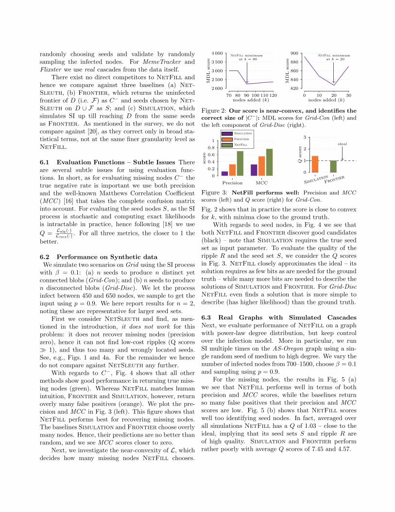
Figure 2: Our score is near-convex, and identifies thecorrect size of |C−|: MDL scores for Grid-Con (left) andthe left component of Grid-Disc (right).

Precision MCC

0

0.2

0.4

0.6

0.8

1

score

Simulation

Frontier

NetFill

Simulati

onFron

tier0

1

2

3

ideal

Qscore

Figure 3: NetFill performs well: Precision and MCCscores (left) and Q score (right) for Grid-Con.

Fig. 2 shows that in practice the score is close to convexfor k, with minima close to the ground truth.

With regards to seed nodes, in Fig. 4 we see thatboth NetFill and Frontier discover good candidates(black) – note that Simulation requires the true seedset as input parameter. To evaluate the quality of theripple R and the seed set S, we consider the Q scoresin Fig. 3. NetFill closely approximates the ideal – itssolution requires as few bits as are needed for the groundtruth – while many more bits are needed to describe thesolutions of Simulation and Frontier. For Grid-DiscNetFill even finds a solution that is more simple todescribe (has higher likelihood) than the ground truth.

6.3 Real Graphs with Simulated CascadesNext, we evaluate performance of NetFill on a graphwith power-law degree distribution, but keep controlover the infection model. More in particular, we runSI multiple times on the AS-Oregon graph using a sin-gle random seed of medium to high degree. We vary thenumber of infected nodes from 700–1500, choose β = 0.1and sampling using p = 0.9.

For the missing nodes, the results in Fig. 5 (a)we see that NetFill performs well in terms of bothprecision and MCC scores, while the baselines returnso many false positives that their precision and MCCscores are low. Fig. 5 (b) shows that NetFill scoreswell too identifying seed nodes. In fact, averaged overall simulations NetFill has a Q of 1.03 – close to theideal, implying that its seed sets S and ripple R areof high quality. Simulation and Frontier performrather poorly with average Q scores of 7.45 and 4.57.

(a) NetSleuth (b) Simulation given true seeds (c) Frontier (d) NetFill

Figure 4: Seeds and Missing Nodes: Performance of NetFill and competitors on Grid-Con. NetSleuth finds nomissing nodes and returns wrong seeds (black). Simulation (given the true seeds) and Frontier (finding good seeds)return overly many false positives (orange). NetFill performs well in both identifying missing nodes (green) as well asrecovers the seeds. Grey nodes are infected, false positives are orange, and false negatives are cyan. Best viewed in color.

6.4 Real Graphs with Real CascadesNext, we use data that defines the infected set D for

us. That is, here we do not simulate the SI modelto construct D. There exist multiple ways to extractthe cascades and the graph. For MemeTracker weconsider two sets of cascades: the Memetracker (MT )methodology of phrase matching, and cascades based onexplicit hyperlinks (HL) [13]. For the graph, we use theHL and MT networks as learnt by NetInf [7]. We thusconsider four combinations of network and infected set:HL-HL, HL-MT , MT -HL and MT -HL.

We select missing nodes using a sampling rate of p =0.7, and choose β = 0.1 – noting that different valueslead to similar results. We use two high-volume memesthat were popular in 2008: “Lipstick on a pig” and “Thestate of the economy”. It is important to emphasize herethat SI is an abstraction; although the network here waslearnt using a SI-inspired model [7], the actual spreadof information in the data may not precisely matchour assumptions. Moreover the network extracted hereusing machine-learning algorithms is itself noisy. Inspite of all this, NetFill discovers interesting results.

For conciseness we only report results for HL-MT ,noting these are representative for the other combina-tions. With respect to missing nodes, NetFill outper-forms the baselines as seen in Fig. 5 (c). Just as for AS-Oregon, Frontier and Simulation perform poorly asthey select almost the entire graph as C−: NetFill’sprecision is more than 5× better than these baselines.With regards to the culprits, Fig. 5 (d) shows the solu-tion discovered by NetFill has a Q score only a frac-tion higher than the ground truth.Truly Missing Nodes: As MemeTracker is itself asample from true cascades in the web, we can applyNetFill on the complete data set with the goal ofdiscovering nodes that were missed when collecting thedata. We used HL-MT using an expected sampling rateof p = 0.9. At this sampling rate NetFill identifies 22nodes (websites) as missing, including ‘nbcbayarea.com’and ‘chicagotribune.com’. By checking their archiveswe verified that 6 sites indeed contain the meme “The

state of the economy”, whereas 2 others discuss politicsand economic situation in USA in general. For theothers verification was not possible – some are not onlineanymore, others do not offer searchable archives.Flixster : Last, we consider the Flixster dataset toevaluate how well NetFill does when the data doesnot follow our assumptions. That is, unlike for Meme-Tracker , for Flixster is unclear whether SI is a meaning-ful model – it is interesting to see whether NetFill stilloutperforms the baselines. In Flixster , the infected setD is a group of people who rated a certain movie, theundirected graph constructed from the friend relation-ship. We consider movies of medium volume infection,|D| ≈ 3000. We used a sampling rate of p = 0.9. Theedge weights were computed following [8], and we setthe infection probability β as the mean edge weight.

We find that NetFill here also outperforms thebaselines in precision, MCC , as well as Q-score with awide margin (figure omitted for brevity) – the differencebeing dramatic for the latter. These scores also showthat NetFill is conservative when the data does notfollow the model, which prevents overfitting and allowsit to find relatively accurate descriptions.Scalability and Robustness Last, but not least, weconsidered the scalability and robustness of NetFill.In short, NetFill is near-linear and robust againstvarying sampling rates. We omit details for brevity.

7 Discussions

The experiments demonstrate that NetFill performsvery well – it obtains high precision and MCC scoresfor both simulated and real-world graphs and cascades– outperforming the baselines by a clear margin. Inter-estingly, NetFill works well even for the MemeTrackerand Flixster datasets – which do not necessarily fol-low the (idealized) SI model, and for which the sam-pling rates are unknown – showcasing the power of ourmethod and formulation.

The small-scale case study for MemeTracker alsoshows that our overall approach works in practice:NetFill recovered 8 truly missing infections from a

Precision MCC

0

0.1

0.2

0.3

0.4

score

Simulation

Frontier

NetFill

(a)

Simulati

onFron

tierNetFi

ll0

2

4

6

8

ideal

Qscore

(b)

Precision MCC

0

0.1

0.2

0.3

0.4

score

(c)

Simulati

onFron

tierNetFi

ll0

1

2

3

ideal

Qscore

(d)

Figure 5: Good performance on real data: AS-Oregon(top) and MemeTracker HL-MT (bottom). NetFill hasbest precision, MCC , and Q scores.

real dataset. It is valid to argue that the SI modelis somewhat simplistic for the type of informationdiffusion in this data. Investigating how NetFill canbe extended towards the richer infection models likeSIR and SEIR, as well as how to incorporate infectiontimestamps will make for engaging future research.

8 Conclusions

In summary, we studied the problem of finding missingnodes and concealed culprits in noisy infected graphs.We approach the problem using compression, and givean efficient method, NetFill, that approximates theideal and automatically recovers both number and iden-tities of missing nodes and seed nodes effectively. Ourmain contributions include:

(a) Problem Formulation: We defined the missing nodeproblem in terms of MDL: the best solution de-scribes the data most succinctly.

(b) Fast Algorithm: We provide a conceptually simpleand fast algorithm, NetFill, which principallyoptimizes our score with an EM-like approach.

(c) Extensive Experiments: NetFill performs verywell on synthetic and real data, even giving mean-ingful results when our assumptions may not hold.

Acknowledgements: This material is based on work sup-

ported by the National Science Foundation under Grant no.

IIS-1353346 and by the Maryland Procurement Office under

contract H98230-14-C0127. JV is supported by the Clus-

ter of Excellence “Multimodal Computing and Interaction”

within the Excellence Initiative of the German Federal Gov-

ernment. Any opinions, findings and conclusions or recom-

mendations expressed in this material are those of the au-

thor(s) and do not necessarily reflect the views of the respec-

tive funding agencies.

References

[1] R. M. Anderson and R. M. May. Infectious Diseases of

Humans. Oxford University Press, 1991.[2] S. P. Borgatti, K. M. Carley, and D. Krackhardt. On

the robustness of centrality measures under conditions of

imperfect data. Soc. Netw., 28(2):124 – 136, 2006.[3] E. Costenbader and T. W. Valente. The stability of

centrality measures when networks are sampled. Soc. Netw.,

25(4):283–307, 2003.[4] T. M. Cover and J. A. Thomas. Elements of Information

Theory. Wiley-Interscience, 2006.[5] M. Faloutsos, P. Faloutsos, and C. Faloutsos. On power-law

relationships of the internet topology. In SIGCOMM, 1999.

[6] M. Gomez-Rodriguez, D. Balduzzi, and B. Scholkopf. Un-covering the temporal dynamics of diffusion networks. In

ICML, 2011.

[7] M. Gomez-Rodriguez, J. Leskovec, and A. Krause. Inferringnetworks of diffusion and influence. In KDD, 2010.

[8] A. Goyal, F. Bonchi, and L. V. Lakshmanan. Learning

influence probabilities in social networks. In WSDM, 2010.[9] P. Grunwald. The Minimum Description Length Principle.

MIT Press, 2007.

[10] G. Kossinets. Effects of missing data in social networks.Soc. Netw., 28(3):247–268, 2006.

[11] A. Lakhina, J. W. Byers, M. Crovella, and P. Xie. Sam-pling biases in ip topology measurements. In In IEEE IN-

FOCOM, pages 332–341, 2003.

[12] T. Lappas, E. Terzi, D. Gunopulos, and H. Mannila.Finding effectors in social networks. In KDD, 2010.

[13] J. Leskovec, L. Backstrom, and J. Kleinberg. Meme

tracking and the dynamics of news cycle. In KDD, 2009.[14] M. Li and P. Vitanyi. An Introduction to Kolmogorov

Complexity and its Applications. Springer, 1993.

[15] A. Maiya and T. Berger-Wolf. Benefits of bias: Towardsbetter characterization of network sampling. In KDD, 2011.

[16] B. Matthews. Comparison of the predicted and observed

secondary structure of T4 phage lysozyme. BBA Prot.Struct., 405(2):442 – 451, 1975.

[17] H. Nishiura, G. Chowell, and C. Castillo-Chavez. Did mod-eling overestimate the transmission potential of pandemic

H1N1-2009? Sample size estimation for post-epidemicseroepidemiological studies. PLoS ONE, 6(3), 03 2011.

[18] B. A. Prakash, J. Vreeken, and C. Faloutsos. Spotting

culprits in epidemics: How many and which ones? In

ICDM. IEEE, 2012.[19] J. Rissanen. Modeling by shortest data description. Annals

Stat., 11(2):416–431, 1983.[20] E. Sadikov, M. Medina, J. Leskovec, and H. Garcia-Molina.

Correcting for missing data in information cascades. In

WSDM. ACM, 2011.

[21] M. Salathe, L. Bengtsson, T. J. Bodnar, D. D. Brewer,J. S. Brownstein, C. Buckee, E. M. Campbell, C. Cattuto,

S. Khandelwal, P. L. Mabry, and A. Vespignani. Digitalepidemiology. PLoS Comput Biol, 8(7), 2012.

[22] D. Shah and T. Zaman. Rumors in a network: Who’s the

culprit? IEEE TIT, 57(8):5163–5181, 2011.[23] L. Wu, X. Ying, X. Wu, and Z.-H. Zhou. Line orthogona-

lity in adjacency eigenspace with application to communitypartition. In IJCAI, 2011.