heuristic optimization to design solar power tower systems · tower systems carmen-ana domínguez...

HEURISTIC OPTIMIZATION TO DESIGN SOLAR POWERTOWER SYSTEMS

Carmen-Ana Domínguez Bravo

July 2016

1. Introduction

2. Optimization problem

3. Analytical and computational model

4. Design of Heliostats Field

5. Design with multiple receivers

THE DESIGN OF ASOLAR POWER TOWER (SPT)

QE

E

O

N

y

z

x

H

Thesis supervisors: Emilio Carrizosa (EIO-US), Enrique Fernández Cara (EDAN-US)Thesis tutor: Manuel Quero (Abengoa Solar)Research contract: CapTorSol 1200-0494 (Abengoa Solar and FIUS)

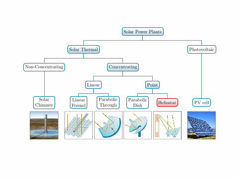
Solar Power Plants

Solar Thermal

Non-Concentrating

SolarChimney

Concentrating

Linear

LinearFresnel

ParabolicThrough

Point

ParabolicDish Heliostat

Photovoltaic

PV cell

SOLAR POWER TOWER PLANTS

I Heliostat: reflective mirror.I Receiver: sunlight collector.

1. Sunlight is reflected by the heliostats fieldonto a receiver at the top of the tower.

2. Thermal energy is transferred through a thermodynamic cycleto produce electricity.

~vsun

Source Abengoa

HELIOSTAT

Helio: Greek word for sun.Stat: stationary (reflected image is fixed).

I Pedestal mounted mirror.I Two-axis tracking system to follow the sun.

Source Abengoa and CIEMAT-PSA

Tower-Receiver(s)

Θ := (h, ξ, α, r)

Heliostats Field

S := {(xi , yi ) ∈ R2 : i ∈ [1,N]}

−400−20002004000

100

200

300

400

500

600

700

800

(West) y coordinate (East)

(So

uth

) x c

oo

rdin

ate

(N

ort

h)

Heliostat Field Layout Nhel

= 624

MATHEMATICAL MODELLINGOPTIMIZATION PROBLEM

(P)

minΘ,S

F (Θ,S) = C(Θ,S)/E(Θ,S)

subject to Θ ∈ Θ

S ∈ S

Π0 ≤ ΠTd (Θ,S) ≤ Π+

I Optimization criteria

I 2 objectives: total construction cost and collected annual energy.

I Deal with the aggregation function,

MATHEMATICAL MODELLING

Tower ( height ), receiver aperture ( position and dimensions ),and heliostats field ( positions and number ).

I Main difficultiesI unknown number of variables,I high number of heliostats in commercial plants (up to 200.000),I expensive objective function evaluation,I nonclosed-form of the objective function,I non-convex constraints.

I AssumptionsI circular aperture,I the aim point is the aperture center and it is static,I the receiver heat flux is homogeneous,I shadowing & blocking effects consider parallel

heliostats,I costs associated with hel. are independent on the

position.

ANALYTICAL AND COMPUTATIONAL MODELCOST FUNCTION

C(h, r , |S|) = β1(h + λ1)λ2 + β2πr 2︸︷︷︸+ cf + c |S|︸︷︷︸I h: tower height.I r : aperture radius.I |S|: number of heliostats.I Tower-receiver and heliostats field costs.I Easy to compute and low number of variables.

ANALYTICAL AND COMPUTATIONAL MODELANNUAL THERMAL ENERGY FUNCTION

I Analytical modelsI Analytical formula and numeric algorithms to evaluate the plant performance.I Accurate enough for the optimization process, e.g. Fortran code NSPOC1.

I Ray-tracing modelsI Tracing light trajectories and simulate the effects of its interactions with digitized objects.I Traditionally used to evaluate the plant performance, e.g. SolTRACE2.

Source Article3.

1L. Crespo and F. Ramos. “NSPOC: A New Powerful Tool for Heliostat Field Layout andReceiver Geometry Optimizations”. In: Proceedings of SolarPaces 2009. 2009

2T. Wendelin. “SolTRACE: A New Optical Modeling Tool for Concentrating Solar Optics”. In:ASME Conference Proceedings. Vol. 2003. 36762. ASME, 2003. DOI:10.1115/ISEC2003-44090

3F. J. Collado and J. Guallar. “A review of optimized design layouts for solar power tower plantswith campo code”. In: Renewable and Sustainable Energy Reviews 20 (2013), pp. 142–154

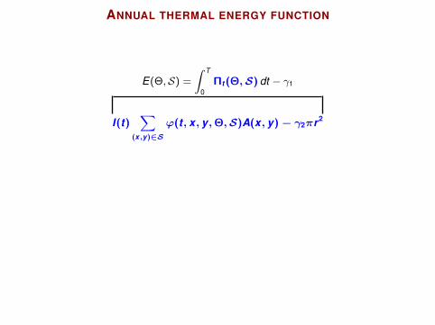
http://dx.doi.org/10.1115/ISEC2003-44090

ANNUAL THERMAL ENERGY FUNCTION

E(Θ,S) =

∫ T

0Πt (Θ,S) dt − γ1

I(t)∑

(x,y)∈S

ϕ(t, x, y,Θ,S)A(x, y)− γ2πr2

I I solar radiation,I A heliostat area,

I ϕ solar efficiency functions:5∏

i=1

νi with νi ∈ [0, 1].

ANNUAL THERMAL ENERGY FUNCTIONSOLAR EFFICIENCY FUNCTIONS

1. Reflectivity constant

2. Cosine√

12 +

~w(x,y)·~vsun(t)2 ||~w(x,y)||

3. Interception f1(t, x, y)∫∫

S exp

(−f2(u,v,x,y)

2 f23 (t,x,y,Θ)

)du dv

4. Atmospheric α1 − α2||~w(x, y)|| + α3||~w(x, y)||2

5. Shading & blocking Sassi’s algorithm1

~v

Source Article2.1G. Sassi. “Some notes on shadow and blockage effects”. In: Solar Energy 31.3 (1983),

pp. 331–3332F. J. Collado and J. Guallar. “A review of optimized design layouts for solar power tower plants

with campo code”. In: Renewable and Sustainable Energy Reviews 20 (2013), pp. 142–154

SOLAR EFFICIENCY FUNCTIONSVARIATIONS

−600 −400 −200 0 200 400 6000

100

200

300

400

500

600

700

800

(South

) x c

oord

inate

(N

ort

h)


Field Distribution: IH 2 ID 3 Ef 2

[0.88833,0.99)

[0.78667,0.88833)

[0.685,0.78667)

[0.58333,0.685)

[0.48167,0.58333)

[0.38,0.48167)

Cosine

−600 −400 −200 0 200 400 6000

100

200

300

400

500

600

700

800

(South

) x c

oord

inate

(N

ort

h)



[0.91833,1)

[0.83667,0.91833)

[0.755,0.83667)

[0.67333,0.755)

[0.59167,0.67333)

[0.51,0.59167)

Interception

−600 −400 −200 0 200 400 6000

100

200

300

400

500

600

700

800

(South

) x c

oord

inate

(N

ort

h)



[0.95333,0.97)

[0.93667,0.95333)

[0.92,0.93667)

[0.90333,0.92)

[0.88667,0.90333)

[0.87,0.88667)

Atmospheric

−600 −400 −200 0 200 400 6000

100

200

300

400

500

600

700

800

(South

) x c

oord

inate

(N

ort

h)



[0.915,1)

[0.83,0.915)

[0.745,0.83)

[0.66,0.745)

[0.575,0.66)

[0.49,0.575)

Shading and blocking

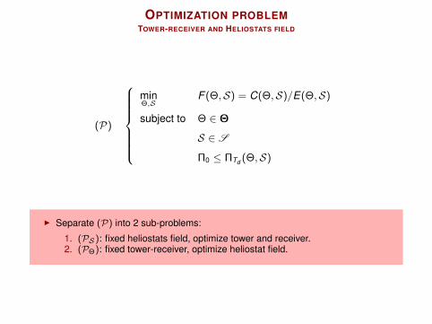
OPTIMIZATION PROBLEMTOWER-RECEIVER AND HELIOSTATS FIELD

(P)

minΘ,S

F (Θ,S) = C(Θ,S)/E(Θ,S)


S ∈ S

Π0 ≤ ΠTd (Θ,S)

I Separate (P) into 2 sub-problems:

1. (PS): fixed heliostats field, optimize tower and receiver.2. (PΘ): fixed tower-receiver, optimize heliostat field.

DESIGN COMPLETE SPT SYSTEM

Optimal Design

(P)

* Tower-Receiver

* Heliostat Field

Alternatingalgorithm

Start

Initial Tower-Receiver Design

Calculate Initial Hel. Field

Optimize Tower-Receiver

Optimize Heliostat Field

Objective valueimproved?

Best Configuration

Stop

No

Yes

DESIGN OF TOWER-RECEIVER

I Receiver variables and feasible set:

I Θ = (h, r , ξ, α),

I Θ ={

Θ ∈ R4 : rmin ≤ r ≤ min(h, rmax) ≤ hmax}

.

y-West

r

z

APERTURE

x-North

ξ

z

RECEIVER

h

dap

Qe

DESIGN TOWER-RECEIVER

(PS) S fixed

max

ΘF (Θ,S) = C(Θ,S)/E(Θ,S)


Π0 ≤ ΠTd (Θ,S)

I Number of variables fixed and low.I Non-convex objective function.I Seems easy to solve (empirically unimodal).

DESIGN TOWER-RECEIVER

(PS) S fixed

max

ΘF (Θ,S) = C(Θ,S)/E(Θ,S)


Π0 ≤ ΠTd (Θ,S)

ResolutionCyclic coordinate method and local searches for each variable.

0.00

0.00

0.00

0.00

0.00

0.00

0.00

0.00

0.00

0.00

0.00

0.00

0.00

0.00

0.00

0.00

0.00

0.00

0.00

0.00

0.00

0.00

29.54

33.42

37.58

41.90

46.17

50.14

53.49

0.00

0.00

0.00

0.00

27.44

30.66

34.05

37.50

40.84

43.85

46.32

0.00

0.00

0.00

0.00

24.65

27.24

29.90

32.53

35.01

37.18

38.90

0.00

0.00

0.00

0.00

21.79

23.81

25.84

27.80

29.59

31.10

32.24

0.00

0.00

0.00

0.00

19.06

20.61

22.12

23.55

24.82

25.86

26.61

0.00

0.00

0.00

0.00

16.55

17.72

18.85

19.88

20.78

21.48

21.96

0.00

0.00

0.00

0.00

14.31

15.19

16.03

16.77

17.40

17.88

18.18

0.00

0.00

0.00

0.00

r ∈ [rmin

,rmax

]

h ∈

[hm

in,h

max

]

F(⋅, S)

1 3.375 5.75 8.125 10.5 12.875 15.25 17.625 20

280

252.1

224.2

196.3

168.4

140.5

112.6

84.7

56.8

28.9

1

DESIGN OF HELIOSTATS FIELD

I Heliostats positions

S ={

(xi , yi ) ∈ R2 : i ∈ [1,N]}

I Feasible set S

rmin ≤√

x2i + y2

i ≤ rmax

||(xi , yi )− (xj , yj )|| ≥ δ−400−2000200400

0

100

200

300

400

500

600

700

800


(South

) x c

oo

rdin

ate

(N

ort

h)


= 624

DESIGN OF HELIOSTATS FIELD

(PΘ) Θ fixed

minS

F (Θ,S) = C(Θ,S)/E(Θ,S)

subject to S ∈ S

Π0 ≤ ΠTd (Θ,S)

I Non-fixed number of variables (expected to be high).I Non-convex objective function.I Non-convex constraints.I Many local optima.

“packing problem with interactions between circles”

DESIGN OF HELIOSTATS FIELDSTATE-OF-THE-ART METHODS: PATTERN-BASED

I Select a geometric pattern (radial-stagger, spiral, grid, etc.)I Pattern described by a low number of parameters.I Optimize the parameters with standard procedures (Powell, Genetic, etc.)

−400−20002004000

100

200

300

400

500

600

700

800


(South

) x c

oord

inate

(N

ort

h)


= 624

Fig: Source Abengoa

DESIGN OF HELIOSTATS FIELDPATTERN-FREE

I Solve future challenges ( flexible algorithm )

Fig: Multiple Receivers.Source Abengoa (Patent US 2012/0125000)

Fig: Multi Tower Solar Array.Source Schramek, 2013.

DESIGN OF HELIOSTATS FIELDPATTERN-FREE

I Solve future challenges ( flexible algorithm )

Greedy algorithm

I greedy-based heuristic

I pattern free to be flexible

I multi-start to avoid local optima

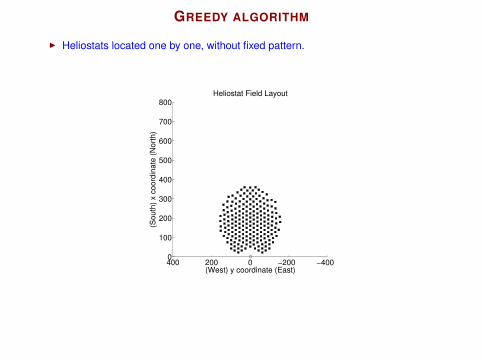
GREEDY ALGORITHM

I Heliostats located one by one, without fixed pattern.

GREEDY ALGORITHM

I Heliostats located one by one, without fixed pattern.I Step k : optimization pb in 2 variables.

I Locate heliostat number kI k − 1 heliostats in the field Sk−1

I Constraints involving Sk−1

(Pk)

max(x,y)∈FS

E(x , y ,Sk−1)

subject to Π0 ≤ ΠTd (Θ,S)

||(x , y)− (x i , y i )|| ≥ δ for i = 1, . . . k − 1

GREEDY ALGORITHM


I Locate heliostat number k .I k − 1 heliostats in the field.I Constraints involving Sk−1.

I Multi-start strategy to avoid local optima.I Nini initial solutions.I Final solution with highest energy value.I Avoid local optima due to shadowing & blocking.


(So

uth

) x c

oo

rdin

ate

(N

ort

h)

Annual Energy Values per unit area

0 0.01 0.02 0.03 0.04 0.05 0.06

GREEDY ALGORITHM



I Multi-start strategy to avoid local optima.I Nini initial solutions.I Final solution with highest energy value.I Avoid local optima due to shadowing & blocking.


(So

uth

) x c

oo

rdin

ate

(N

ort

h)

Annual Energy Values per unit area with S and B

0 0.01 0.02 0.03 0.04 0.05 0.06

GREEDY ALGORITHM



I Multi-start strategy to avoid local optima.I Nini initial solutions.I Final solution with highest energy value.I Avoid local optima due to shadowing & blocking effects.

−400 −300 −200 −100 0 100 200 300 4000

100

200

300

400

500

600

700

800


(So

uth

) x c

oo

rdin

ate

(N

ort

h)


= 624

−400 −300 −200 −100 0 100 200 300 4000

100

200

300

400

500

600

700

800


(So

uth

) x c

oo

rdin

ate

(N

ort

h)


= 624

GREEDY ALGORITHM



I Multi-start strategy to avoid local optima.I Nini different random solutions.I Perform local search.I Final solution, the one with highest energy value.

I Determine the final number of heliostats.I Π0 ≤ ΠTd (x , y ,Sk−1)→ feasible solution.I Continue locating heliostats.I Stop when the objective function C/E does not improve.I Final N.

GREEDY ALGORITHM

I Heliostats located one by one, without fixed pattern.

−400−20002004000

100

200

300

400

500

600

700

800


(South

) x c

oord

inate

(N

ort

h)

Heliostat Field Layout

DESIGN OF HELIOSTATS FIELDCOMPARATIVE RESULTS

Radial-staggered1

−400−20002004000

100

200

300

400

500

600

700

800


(South

) x c

oord

inate

(N

ort

h)


= 624

Spiral2

−400−20002004000

100

200

300

400

500

600

700

800


(South

) x c

oord

inate

(N

ort

h)


= 624

Greedy3

−400−20002004000

100

200

300

400

500

600

700

800


(South

) x c

oord

inate

(N

ort

h)


= 624

1L. L. Vant-Hull. Layout of optimized Heliostat Field. Tech. rep. University of Houston, 19912C. J. Noone, M. Torrilhon, and A. Mitsos. “Heliostat field optimization: A new computationally

efficient model and biomimetic layout”. In: Solar Energy 86 (2012), pp. 792–8033E. Carrizosa et al. “A heuristic method for simultaneous tower and pattern-free field optimization

on solar power systems”. In: Computers & Operations Research 57 (2015), pp. 109–122

DESIGN OF HELIOSTATS FIELDCOMPARATIVE RESULTS

Field N ΠTd E F

PS10 624 0.43 0.12 0.0120

Spiral 624 0.42 0.12 0.0120

GPS10 Requirement Phase 624 0.43 0.12 0.0120

GPS10 Completion Phase 943 0.62 0.17 0.0111

Thermal power at Td , ΠTd(MWth 10−2).

Annual thermal energy, E (GWHth 10−3).Cost function, C (Me),

Cost per unit of annual thermal energy, F = C/E .

DIFFERENT FEASIBLE REGIONSRECTANGULAR, PERFORATED AND VALLEY REGIONS


(Sou

th)

x co

ordi

nate

(N

orth

)

Feasible Region 1


(Sou

th)

x co

ordi

nate

(N

orth

)

Feasible Region 2


(Sou

th)

x co

ordi

nate

(N

orth

)

Feasible Region 3

−400 −300 −200 −100 0 100 200 300 4000

100

200

300

400

500

600

700

800


(South

) x c

oord

inate

(N

ort

h)


= 611

(d) PS10

−400 −300 −200 −100 0 100 200 300 4000

100

200

300

400

500

600

700

800


(South

) x c

oord

inate

(N

ort

h)


= 607

(e) Requirement

−400 −300 −200 −100 0 100 200 300 4000

100

200

300

400

500

600

700

800


(South

) x c

oord

inate

(N

ort

h)


= 745

(f) Completion

−400 −300 −200 −100 0 100 200 300 4000

100

200

300

400

500

600

700

800


(South

) x c

oord

inate

(N

ort

h)


= 611

(g) RPS10

−400 −300 −200 −100 0 100 200 300 4000

100

200

300

400

500

600

700

800


(South

) x c

oord

inate

(N

ort

h)


= 612

(h) Requirement

−400 −300 −200 −100 0 100 200 300 4000

100

200

300

400

500

600

700

800

(West) y coordinate (East)(S

ou

th)

x c

oo

rdin

ate

(N

ort

h)


= 824

(i) Completion

DIFFERENT FEASIBLE REGIONSRECTANGULAR, PERFORATED AND VALLEY REGIONS

PS10

Reg S |S| ΠTdΠ+ E F Fsep

R

Orig. 420 0.29 - 0.080 0.01362 -

Req. 419 0.29 0.31 0.079 0.01362 1.5

Compl. (Π+) - - 0.31 - - 1.5

Compl. 425 0.30 - 0.081 0.01333 1.5

P

Orig. 611 0.42 - 0.11 0.012 -

Req. 607 0.42 0.44 0.11 0.012 1.5

Compl.(Π+) 639 0.44 0.44 0.12 0.012 1.5

Compl. 745 0.50 - 0.14 0.01152 1.5

V

Orig. 565 0.38 - 0.11 0.01224 -

Req. 562 0.38 0.40 0.10 0.01248 1.6

Compl. (Π+) 592 0.40 0.40 0.11 0.01224 1.6

Compl. 856 0.56 - 0.15 0.01134 1.6

Thermal power at Td , ΠTd(MWth 10−2).

Annual thermal energy, E (GWHth 10−3).Cost function, C (Me),


MORE PROBLEMS

Heliostat pods 1

−30 −20 −10 0 10 20 30−50

−40

−30

−20

−10

0

(West) x coordinate (East)

(So

uth

) y c

oo

rdin

ate

(N

ort

h)

Genetic−based Heliostat Field Layout

Multi-size-heliostats 2

−400−20002004000

100

200

300

400

500

600

700

800


(South

) x c

oord

inate

(N

ort

h)

Heliostat Field Layout N1hel

= 491 N2hel

=3647

Multiple receivers3

−1000−50005001000

−200

0

200

400

600

800

1000


(South

) x c

oord

inate

(N

ort

h)


= 1872

1C. Domínguez-Bravo et al. “Field-design optimization with triangular heliostat pods”. In:Proceedings of SolarPaces 2015. 2015

2E. Carrizosa et al. An Optimization Approach to the Design of Multi-Size-Heliostat fields.Tech. rep. www.optimization-online.org/DB_HTML/2014/05/4372.html. IMUS, 2014

3E. Carrizosa et al. “Optimization of multiple receivers Solar Power Tower systems”. In: Energy90 (2015), pp. 2085–2093

MULTIPLE RECEIVERS

One receiver(northern

or southern field)

Source Abengoa (SP20)

Circular receiver(surrounding field)

Source TorresolEnergy (Gemasolar)

Multiple receivers(separate fields)

Source Abengoa

(Patent US 2012/0125000)

MULTIPLE RECEIVERSOPTIMIZATION PROBLEM

(P)

minΘ,S

F (Θ,S)


S ∈ S

Π−i ≤ ΠTd (Θi ,S) ≤ Π+i i = 1, 2, 3

I F = C/E .I i = 1, 2, 3, receivers.I Θ = (Θ1,Θ2,Θ3) with Θi = (ri , hi , ξi , αi )

t ∈ R4 ∀ i .

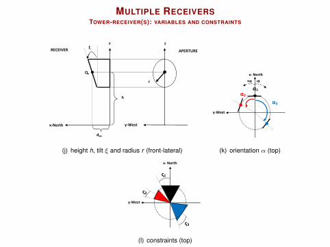
MULTIPLE RECEIVERSTOWER-RECEIVER(S): VARIABLES AND CONSTRAINTS

y-West

r

z

APERTURE

x-North

ξ

z

RECEIVER

h

dap

Qe

(j) height h, tilt ξ and radius r (front-lateral)

+α -α

x- North

y-West

α1

α3

α2

(k) orientation α (top)

x- North

y-West

ς1

ς2

ς3

(l) constraints (top)

MULTIPLE RECEIVERSHELIOSTATS FIELD PROBLEM

(PΘ) Θ fixed

minS

F (Θ,S)

subject to S ∈ S

Π−i ≤ ΠTd (Θi ,S) ≤ Π+i i = 1, 2, 3

I Assumptions:

1. Separate fields: each receiver have a separate field region.S = S1 ∪ S2 ∪ S3 and S1 ∩ S2 ∩ S3 = ∅Si = {(x , y) ∈ S : heliostat at (x , y) aims at receiver i}

2. Static aiming strategy: heliostats always aim to the same receiver.

MULTIPLE RECEIVERSSTATE-OF-THE-ART

Dual receiver4

Two integrated receivers(external and cavity)5 Multiple apertures6

4Y. Luo, X. Du, and D. Wen. “Novel design of central dual-receiver for solar power tower”. In:Applied Thermal Engineering 91 (2015), pp. 1071–1081

5R. Ben-Zvi, M. Epstein, and A. Segal. “Simulation of an integrated steam generator for solartower”. In: Solar Energy 86 (2012), pp. 578–592

6M. Schmitz et al. “Assesment of the potencial improvement due to multiple apertures in centralreceiver systems with secondary concentrators”. In: Solar Energy 80 (2006), pp. 111–120

MULTIPLE RECEIVERS

Algorithm steps

1. Calculate aiming regions: S1,S2 and S3.

2. Locate the heliostats:2.1 Complete North region.2.2 Update boundaries.2.3 Complete West & East simultaneously.

MULTIPLE RECEIVERS

Calculate aiming regions:

1. Discretization of the feasible region.

2. At each point, calculate energy values for each receiver.

3. Select boundary points and obtain polynomial boundaries.

4. Different possibilities applying weights.


(So

uth

) x c

oo

rdin

ate

(N

ort

h)

Best Annual Energy Values

0 1 2 3 4 5 6 7

MULTIPLE RECEIVERS







(So

uth

) x c

oo

rdin

ate

(N

ort

h)

Best Annual Energy Values

0 1 2 3 4 5 6 7

−1000 −800 −600 −400 −200 0 200 400 600 800 1000−1000

−800

−600

−400

−200

0

200

400

600

800

1000


(So

uth

) x c

oo

rdin

ate

(N

ort

h)

Regions of a Multi−receiver Field

MULTIPLE RECEIVERS






−1000 −800 −600 −400 −200 0 200 400 600 800 1000−1000

−800

−600

−400

−200

0

200

400

600

800

1000


(So

uth

) x c

oo

rdin

ate

(N

ort

h)


MULTIPLE RECEIVERS






−1000 −800 −600 −400 −200 0 200 400 600 800 1000−1000

−800

−600

−400

−200

0

200

400

600

800

1000


(So

uth

) x c

oo

rdin

ate

(N

ort

h)


−1000−50005001000−1000

−500

0

500

1000


(So

uth

) x c

oo

rdin

ate

(N

ort

h)

Field Regions with Three Receivers

p(x) W

q(x) E

Data W

Data E

MULTIPLE RECEIVERS






−1000−50005001000−1000

−500

0

500

1000


(So

uth

) x c

oo

rdin

ate

(N

ort

h)


p(x) W

q(x) E

Data W

Data E

MULTIPLE RECEIVERS






−1000−50005001000−1000

−500

0

500

1000


(So

uth

) x c

oo

rdin

ate

(N

ort

h)


p(x) W

q(x) E

Data W

Data E

−1000−50005001000−1000

−500

0

500

1000


(So

uth

) x c

oo

rdin

ate

(N

ort

h)


1.010 W

1.010 E

1.005 W

1.005 E

1 W

1 E

0.995 W

0.995 E

0.990 W

0.990 E

Data W

Data E

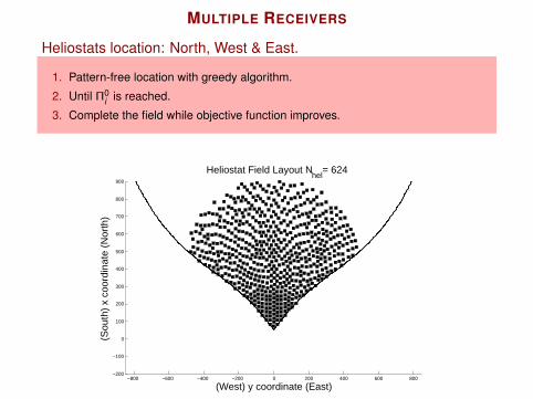
MULTIPLE RECEIVERS

Heliostats location: North, West & East.

1. Pattern-free location with greedy algorithm.

2. Until Π0i is reached.

3. Complete the field while objective function improves.

−800 −600 −400 −200 0 200 400 600 800−200

−100

0

100

200

300

400

500

600

700

800

900


(Sou

th)

x co

ordi

nate

(N

orth

)


= 624

MULTIPLE RECEIVERS

Heliostats location: North, West & East.

1. Pattern-free location with greedy algorithm.

2. Until Π0i is reached.

3. Complete the field while objective function improves.

−800 −600 −400 −200 0 200 400 600 800−200

−100

0

100

200

300

400

500

600

700

800

900


(Sou

th)

x co

ordi

nate

(N

orth

)


= 1872

MULTIPLE RECEIVERSALTERNATING ALGORITHM

Step Pb |S| ΠTd E C F

k = 0 1 : (Θ0,S0) 2009 118.7550 326.83 5.9984 0.01835

2 : (Θ1,S0) 2009 112.0731 310.62 5.3916 0.01736

k = 1 3 : (Θ1,S1) 2033 115.0178 314.55 5.4445 0.01731

4 : (Θ2,S1) 2033 110.4583 306.45 5.3443 0.01744

k = 2 5 : (Θ2,S2) 2084 114.8432 312.30 5.4567 0.01747

Thermal power at Td , ΠTd(MWth).

Annual thermal energy, E (GWHth).Cost function, C (Me).


MULTIPLE RECEIVERSALTERNATING ALGORITHM: RECEIVERS

Step h ξ α r

Θ0

Θ1 100.50 12.50 0 6.39

Θ2 100.50 12.50 90 6.39

Θ3 100.50 12.50 −90 6.39

Θ1 100.53 8.72 −0.81 4.83

Θ2 100.50 17.24 80.94 4.44Θ1

Θ3 100.50 17.96 −81.32 4.48

Θ2

Θ1 100.50 10.71 −0.26 4.44

Θ2 100.50 17.50 75.41 4.11

Θ3 100.50 17.43 −76.09 4.11

Tower height, h (m).

Receiver aperture tilt ξ (grad), orientation α (grad) and radius r (m).

MULTIPLE RECEIVERSALTERNATING ALGORITHM: FIELDS

−1000−50005001000

−200

0

200

400

600

800

1000


(South

) x c

oord

inate

(N

ort

h)


= 2009

−1000−50005001000

−200

0

200

400

600

800

1000


(South

) x c

oord

inate

(N

ort

h)


= 2033

−1000−50005001000

−200

0

200

400

600

800

1000


(South

) x c

oord

inate

(N

ort

h)


= 2084

Eskerrik [email protected]

REFERENCES I[1] Pat. US 2012 0125000 A1. 2012.

[2] L. Alon et al. “Computer-Based Management of Mirror-Washing in Utility-Scale Solar Thermal Plants”. In: Proceedings of ASME2014 (8th International Conference on Energy Sustainability and 12th International Conference on Fuel Cell Science, Engineeringand Technology). Vol. 1. ES2014-6562. 2014.

[3] L. Amsbeck et al. “Optical Performance and Weight Estimation of a Heliostat With Ganged Facets”. In: Journal of Solar EnergyEngineering 130.011010 (2008), (3 Pages).

[4] R. Ben-Zvi, M. Epstein, and A. Segal. “Simulation of an integrated steam generator for solar tower”. In: Solar Energy 86 (2012),pp. 578–592.

[5] S. M. Besarati, D. Y. Goswami, and E. K. Stefanakos. “Optimal heliostat aiming strategy for uniform distribution of heat flux on thereceiver of a solar power tower plant”. In: Energy Conversion and Management 84 (2014), pp. 234–243.

[6] J. B. Blackmon. “Parametric determination of heliostat minimum cost per unit area”. In: Solar Energy 97 (2013), pp. 342–349.

[7] P. Cádiz et al. “Shadowing and blocking effect optimization for a variable geometry heliostat field”. In: Energy Procedia 69 (2015),pp. 60–69.

[8] E. Carrizosa et al. “A heuristic method for simultaneous tower and pattern-free field optimization on solar power systems”. In:Computers & Operations Research 57 (2015), pp. 109–122.

[9] E. Carrizosa et al. An Optimization Approach to the Design of Multi-Size-Heliostat fields. Tech. rep.www.optimization-online.org/DB_HTML/2014/05/4372.html. IMUS, 2014.

[10] E. Carrizosa et al. “Optimization of multiple receivers Solar Power Tower systems”. In: Energy 90 (2015), pp. 2085–2093.

[11] F. J. Collado and J. Guallar. “A review of optimized design layouts for solar power tower plants with campo code”. In: Renewableand Sustainable Energy Reviews 20 (2013), pp. 142–154.

[12] L. Crespo and F. Ramos. “NSPOC: A New Powerful Tool for Heliostat Field Layout and Receiver Geometry Optimizations”. In:Proceedings of SolarPaces 2009. 2009.

[13] C. Domínguez-Bravo et al. “Field-design optimization with triangular heliostat pods”. In: Proceedings of SolarPaces 2015. 2015.

[14] M. Izygon et al. “TieSOL – A GPU-based suite of fsoftware for central receiver solar power plants”. In: Proceedings of SolarPaces2011. 2011.

[15] J. Larmuth, K. J. Malan, and P. Gauché. Design and Cost Review of 2 m2 Heliostat Prototypes. Tech. rep.http://concentrating.sun.ac.za/wp-content/uploads/2014/02/52.pdf. STERG, Stellenbosch University, 2014.

[16] Y. Luo, X. Du, and D. Wen. “Novel design of central dual-receiver for solar power tower”. In: Applied Thermal Engineering 91(2015), pp. 1071–1081.

REFERENCES II

[17] T. R. Mancini. Catalog of Solar Heliostats. Tech. rep. III–1/00. SolarPaces, 2000. URL:www.fika.org/jb/resources/Heliostat\%20Catalog.pdf.

[18] C. J. Noone, M. Torrilhon, and A. Mitsos. “Heliostat field optimization: A new computationally efficient model and biomimetic layout”.In: Solar Energy 86 (2012), pp. 792–803.

[19] C. J. Noone et al. “Site selection for hillside central receiver solar thermal plants”. In: Solar Energy 85 (2011), pp. 839–848.

[20] A. Ramos and F. Ramos. “Heliostat blocking and shadowing efficiency in the video-game era”. arXiv:1402.1690v1. 2014. URL:http://arxiv.org/pdf/1402.1690.pdf.

[21] P. Ricklin et al. “Commercial readiness of eSolar next generation heliostat”. In: Energy Procedia 49 (2014). SolarPaces 2013,pp. 201–208.

[22] G. Sassi. “Some notes on shadow and blockage effects”. In: Solar Energy 31.3 (1983), pp. 331–333.

[23] M. Schmitz et al. “Assesment of the potencial improvement due to multiple apertures in central receiver systems with secondaryconcentrators”. In: Solar Energy 80 (2006), pp. 111–120.

[24] P. Schramek and D. R. Mills. “Multi-tower solar array”. In: Solar Energy 75.3 (2003), pp. 249–260.

[25] J. Spelling et al. “Thermoeconomic optimization of a combined-cycle solar tower power plant”. In: Energy 41 (2012), pp. 113–120.

[26] L. L. Vant-Hull. Layout of optimized Heliostat Field. Tech. rep. University of Houston, 1991.

[27] T. Wendelin. “SolTRACE: A New Optical Modeling Tool for Concentrating Solar Optics”. In: ASME Conference Proceedings.Vol. 2003. 36762. ASME, 2003. DOI: 10.1115/ISEC2003-44090.

www.fika.org/jb/resources/Heliostat\%20Catalog.pdf

http://arxiv.org/pdf/1402.1690.pdf

http://dx.doi.org/10.1115/ISEC2003-44090

heuristic optimization to design solar power tower systems · tower systems carmen-ana domínguez...

Documents