heuristic algorithms for solving problem that involves ... · pdf filethis chapter will...

The candidate confirms that the work submitted is their own and the appropriate credit has been givenwhere reference has been made to the work of others.

I understand that failure to attribute material which is obtained from another source may be consideredas plagiarism.

(Signature of student)

Heuristic algorithms for solvingproblem that involves production

scheduling and transportationJi Hyun YoonComputing

Session 2004/2005

1

Summary

The aim of this project is to produce heuristic algorithms for integrated problems of

scheduling and transportation. The objectives are to construct for both production and

transportation schedule. The algorithms which have been designed are implemented for

computational experiments to analyse the performance.

2

Acknowledgements

I would like to thank my supervisor Dr Natasha Shakhlevich for giving me help and guidance for this

project.

3

Contents

Chapter 1 Introduction 1 1.1 Introduction 1

1.2 Aim 2

1.3 Minimum Requirements 2

1.4 Project Schedule 2

Chapter 2 Background Research 5

2.1 Scheduling Algorithms 5

2.2 Heuristic Algorithms 6

2.3 Exact Algorithm 7

2.4 Computational Complexity 7

2.5 Outline of the Problem 8

2.6 Batching Problems 14

Chapter 3 Algorithm Design 15

3.1 Special cases 15

3.2 Design 16

3.3 Evaluation criteria and time complexity 20

Chapter4 Algorithm Implementation 22

4.1 Input and Output 22

4.2 Testing 25

Chapter 5 Computational Experiments 26

5.1 Introduction 26

5.2 Algorithms Used 27

5.3 Results 27

Chapter 6 Evaluations 32

6.1 Minimum requirements 32

6.2 Evaluation of the algorithms 32

6.3 Summary 37

Chapter7 Conclusions and Future Work 38

4

7.1 Review of the Project 38

7.2 Conclusion 38

7.3 Future Work 39

Bibliography 42

Appendix A 43

5

Chapter 1

Introduction

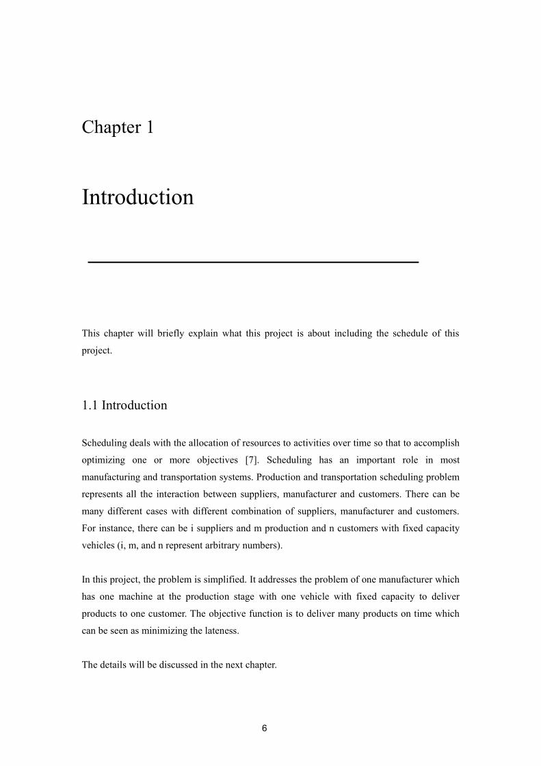
This chapter will briefly explain what this project is about including the schedule of this

project.

1.1 Introduction

Scheduling deals with the allocation of resources to activities over time so that to accomplish

optimizing one or more objectives [7]. Scheduling has an important role in most

manufacturing and transportation systems. Production and transportation scheduling problem

represents all the interaction between suppliers, manufacturer and customers. There can be

many different cases with different combination of suppliers, manufacturer and customers.

For instance, there can be i suppliers and m production and n customers with fixed capacity

vehicles (i, m, and n represent arbitrary numbers).

In this project, the problem is simplified. It addresses the problem of one manufacturer which

has one machine at the production stage with one vehicle with fixed capacity to deliver

products to one customer. The objective function is to deliver many products on time which

can be seen as minimizing the lateness.

The details will be discussed in the next chapter.

6

1.2 Aim

The overall aim of the project is to produce heuristic algorithms for integrated problems of

scheduling and transportation. The objectives of the project are to construct both production

and transportation schedule.

1.3 Minimum Requirements

To describe the scheduling model that involves transportation

To design algorithms for scheduling production and transportation

To implement one algorithm in C++ for scheduling production and transportation

To perform computational experiments and to analyse the performance of the

algorithm

The possible extensions which were mentioned in mid-project report are stated below.

Implementing several additional heuristic algorithms

Design of a local search algorithm

Design of exact algorithms for the special cases of the problem

Generalising the heuristic algorithms for solving more complex problems

1.4 Project Schedule

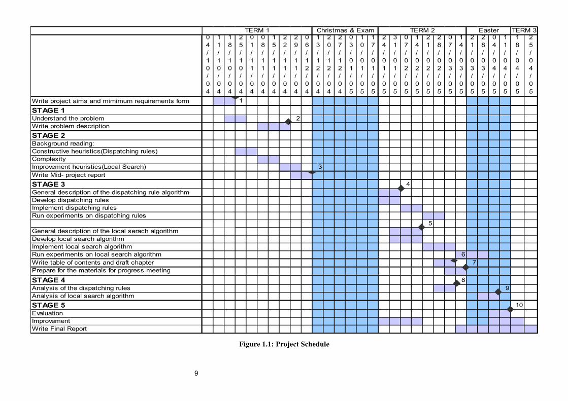
The project schedule is represented as a Gantt chart (see Figure 1.1) to show the progress. It

has several milestones which measure the efficiency of the project.

Milestones:

1: project aim and minimum requirement

2: problem description

3: mid-project project

7

M

4: description of algorithm for dispatching rules

5: description of algorithm for local search

6: table of contents and draft chapter

7: materials for progress meeting

8: analysis the dispatching rule

9: analysis the local search method

8

04/10/04

11/10/04

18/10/04

25/10/04

01/11/04

08/11/04

15/11/04

22/11/04

29/11/04

06/12/04

13/12/04

20/12/04

27/12/04

03/01/05

10/01/05

17/01/05

24/01/05

31/01/05

07/02/05

14/02/05

21/02/05

28/02/05

07/03/05

14/03/05

21/03/05

28/03/05

04/04/05

11/04/05

18/04/05

25/04/05

Write project aims and mimimum requirements form 1

STAGE 1Understand the problem 2Write problem descriptionSTAGE 2Background reading:Constructive heuristics(Dispatching rules)ComplexityImprovement heuristics(Local Search) 3Write Mid- project reportSTAGE 3 4General description of the dispatching rule algorithmDevelop dispatching rulesImplement dispatching rulesRun experiments on dispatching rules

5General description of the local serach algorithmDevelop local search algorithmImplement local search algorithmRun experiments on local search algorithm 6Write table of contents and draft chapter 7Prepare for the materials for progress meeting

STAGE 4 8Analysis of the dispatching rules 9Analysis of local search algorithmSTAGE 5 10EvaluationImprovementWrite Final Report

TERM 3Christmas & Exam EasterTERM 1 TERM 2

M

M

M

Figure 1.1: Project Schedule

9

Chapter 2

Background Research

2.1 Scheduling Algorithms

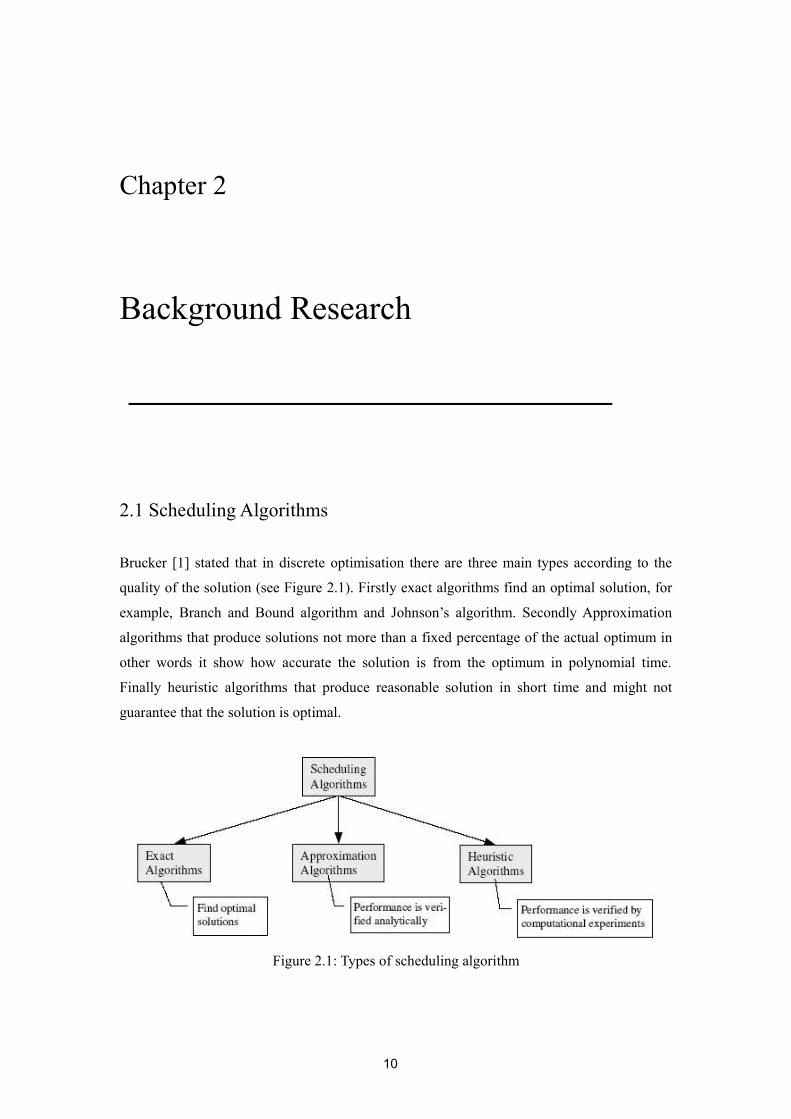
Brucker [1] stated that in discrete optimisation there are three main types according to the

quality of the solution (see Figure 2.1). Firstly exact algorithms find an optimal solution, for

example, Branch and Bound algorithm and Johnson’s algorithm. Secondly Approximation

algorithms that produce solutions not more than a fixed percentage of the actual optimum in

other words it show how accurate the solution is from the optimum in polynomial time.

Finally heuristic algorithms that produce reasonable solution in short time and might not

guarantee that the solution is optimal.

Figure 2.1: Types of scheduling algorithm

10

2.2 Heuristic Algorithms

As mentioned above heuristic algorithms can find a reasonably good solution in a relatively

fast time. Other advantages are that they are very simple to implement and can find optimal

solutions for special cases. On the other hand, disadvantages are that in practice the

algorithms are used limitedly as it can find unpredictably bad solution.

Pinedo [2] discussed the theory of heuristic methods such as constructive heuristic (e.g.

dispatching rules) which will be used for computational experiments and improvement

heuristics (e.g. local search method).

2.2.1 Construction Heuristics

Construction heuristics start with an empty schedule and add one job at a time. Dispatching

rules are an example of this heuristic. All the jobs waiting to be processed by the machine are

prioritised. So when the machine is free the job with the highest priority will be processed.

Some well known dispatching rule are listed in Table 2 from Pinedo [7].

Table 1: Dispatching Rules

One of the dispatching rules is EDD rule (Earliest Release Date) where the jobs are ordered

in non-decreasing order of the due date.

11

2.2.2 Improvement Heuristics

Improvement heuristics start with a schedule and try to find a better schedule S’ based on the

initial schedule S by generating neighbours iteratively. Local search method is an example of

such as this heuristic approach. Local search have two different category iterative algorithm

and genetic algorithm. The former uses neighbourhood search method while the latter

operates with a population of schedules. Four major iterative algorithms can be used to

improve current schedule. These are iterative improvement, threshold accepting, simulated

annealing and tabu search. The problem will use threshold accepting so the rest of local

search method will not be discussed.

Neighbourhood search methods comprise four steps.

Step 1: Initialisation – Choose an initial schedule S and compute the objective function F(S).

Step 2: Neighbourhood Generation – Select a neighbour S’ from the current solution S and

compute F(S’)

Step 3: Acceptance Test – Test whether to accept to move from S to S’. If acceptable, then S’

replaces S if not move to next step.

Step 4: Termination Test – Test whether to terminate the search procedure. If it terminates,

output the best solution generated if not return to neighbourhood generation (Step 2).

2.3 Exact Algorithm

Exact algorithm guarantee to find an optimal solution. However the algorithm is extremely

slow since the problem is NP-hard. Computational complexity will be discussed later on. The

most commonly used exact algorithm is branch and bound algorithm. It will save time if the

initial schedule starts with a good solution because many branches can be eliminated.

2.4 Computational Complexity

Pinedo [7] stated the brief overview of the complexity theory which will be used in analysing

the algorithms. Complexity theory is used to classify the problem as easy or hard to solve. If

the problem can be solved in polynomial time than it is called class P, otherwise it is ΝP-

hard. Efficient algorithm exists for P problem. ΝP-hard problem is intractable and is unlikely

that a polynomial-time algorithm exists.

12

The objective function of this project is minimising maximum lateness which is strongly NP-

hard whereas 1||Lmax problem is polynomial solvable. The problem 1|rj|Lmax is a special case of

1||Lmax with given release date.

Pinedo [7] commented that 1|rj|Lmax problem is important for flow shop problem because of its

numerous appearances as sub problem in heuristic procedures.

2.5 Outline of the Problem

Some papers have been written about production and transportation scheduling problem [3],

[4], [6]. But those papers did not cover the simplified model which is going to be solved.

2.5.1 Classical Scheduling Problem

In general, classical scheduling problem also known as pure scheduling problem which has

no transportation issue where a manufacturer should schedule the jobs given all the

information such as processing times, release dates and due dates. However, there are other

problems which involve the transportation issue. These problems are machine scheduling

with transportation coordination and job delivery coordination. Below is the problem

simplified based on the classical scheduling problem.

2.5.2 Production and Transportations Scheduling Problem

The production and transportation problem represents all the interaction between suppliers,

manufacturers and customers. For example, jobs are released from the supplier to the

manufacturer to be processed by machines and delivered by vehicles to the customers by the

due dates where each vehicle has a capacity constraint.

The problem is to construct the production schedule and the transportation schedule using

heuristic algorithms. The objective function is minimizing maximum lateness depends on the

due date [7].

In this project, we consider the following simplified model. There is one manufacture with a

13

single machine; one customer site, one vehicle to deliver the jobs but no suppliers.

Notations can be defined as below:

j – job numbers

n - number of jobs

pj – processing time of job j on a single machine without interruption

rj - release time of job j

dj - due date of job j to the customer

v - capacity of the vehicle (The maximum number of items that the vehicle can

carry.)

t - transportation time of vehicle from manufacturer to customer

r – return time of vehicle from customer to manufacturer

Notation of Scheduling Problem: α | β | γ

α – machine environment

β – constraints or job characteristics

γ – objective to be minimised(optimality criteria)

Constraints:

Release time – the earliest allowed start time, the job shouldn’t be allowed to be

processed before the release time

Processing time – the time the job spends on a machine, since pre-emption is not

allowed the job must finish processing before another job start

Due date – the time the job is promised to the customer

Optimal Criteria:

Cpj – completion time for productions schedule

Ctj – the finished time of delivery of job j for transportation schedule

Lj – lateness of job j

Lj = Ctj - dj

Positive if the job is completed before due date, otherwise negative

Lmax – maximum of lateness

Lmax = max(L1, L2,, …, Ln)

14

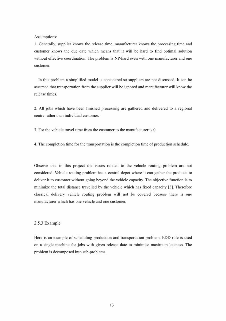
Assumptions:

1. Generally, supplier knows the release time, manufacturer knows the processing time and

customer knows the due date which means that it will be hard to find optimal solution

without effective coordination. The problem is NP-hard even with one manufacturer and one

customer.

In this problem a simplified model is considered so suppliers are not discussed. It can be

assumed that transportation from the supplier will be ignored and manufacturer will know the

release times.

2. All jobs which have been finished processing are gathered and delivered to a regional

centre rather than individual customer.

3. For the vehicle travel time from the customer to the manufacturer is 0.

4. The completion time for the transportation is the completion time of production schedule.

Observe that in this project the issues related to the vehicle routing problem are not

considered. Vehicle routing problem has a central depot where it can gather the products to

deliver it to customer without going beyond the vehicle capacity. The objective function is to

minimize the total distance travelled by the vehicle which has fixed capacity [3]. Therefore

classical delivery vehicle routing problem will not be covered because there is one

manufacturer which has one vehicle and one customer.

2.5.3 Example

Here is an example of scheduling production and transportation problem. EDD rule is used

on a single machine for jobs with given release date to minimise maximum lateness. The

problem is decomposed into sub-problems.

15

Figure 2.1 Classical Scheduling problem

Above is a simplified problem where no suppliers and customers so that the manufacturer

have the information about release date, processing time and due date.

Manufacturer has a single machine with one vehicle. The capacity of the vehicle v is 3.

Transportation time (i.e. TransTime) of the vehicle is 20. It is assumed pre-emption is not

allowed and the vehicle travel time (i.e. ReturnTime) from the customer to the manufacture is

0.

Input data:

The general diagram of the problem is shown below.

capacity = 3

TransTime = 20

ReturnTime = 0

j pj rj dj

1 8 0 412 4 5 463 4 10 604 7 11 505 10 21 62

j dj

1 412 463 604 505 62

CustomerManufacturer

Vehicle

Production

16

j pj rj

1 8 02 4 53 4 104 7 115 10 21

[Table 2]Data for the production with

processing time, release time of job j.

[Table 3]Data for the customer with due

date of job j.

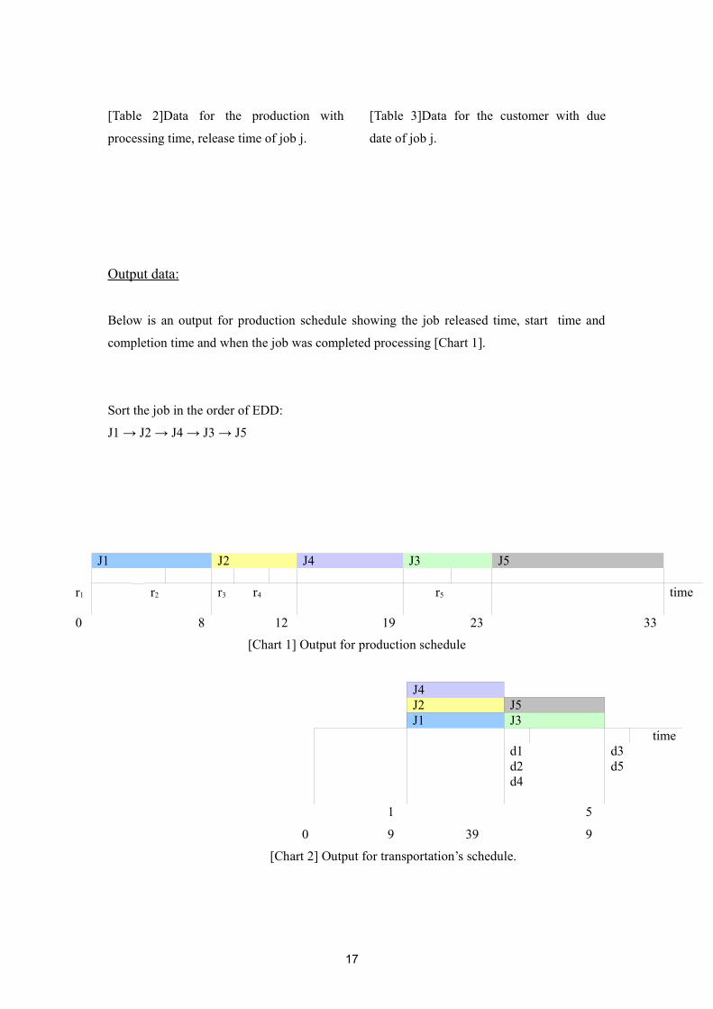
Output data:

Below is an output for production schedule showing the job released time, start time and

completion time and when the job was completed processing [Chart 1].

Sort the job in the order of EDD:

J1 → J2 → J4 → J3 → J5

J1 J2 J4 J3 J5　　　　　　　　　　　　　　　　　　　　　　　　　　　　　　　　　　　　

r1 　　　　r2 　　　 r3 r4 　　 r5 　　 time　　　　　　

0 8 12 19 23 33

[Chart 1] Output for production schedule

J4 　　　　　J2 J5

　　　　　 J1 J3 　　　　　　　　　　　　　　 time

　　　 d1 　 d3　　　 d2 　 d5　　　 d4 　　　　　

0

1

9 39

5

9

[Chart 2] Output for transportation’s schedule.

17

When three jobs are available the vehicle delivers the jobs as batches to the customer. Since

the vehicle capacity is three.

Chart 2 illustrates an output for transportation’s schedule showing the job due date and when

the job was delivered to customer.

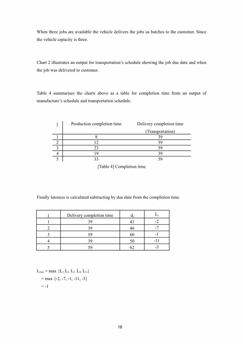
Table 4 summarises the charts above as a table for completion time from an output of

manufacture’s schedule and transportation schedule.

j Production completion time Delivery completion time

(Transportation)1 8 392 12 393 23 594 19 395 33 59

[Table 4] Completion time

Finally lateness is calculated subtracting by due date from the completion time.

j Delivery completion time dj Lj

1 39 41 -22 39 46 -73 59 60 -14 39 50 -115 59 62 -3

Lmax = max {L1, L2, L3, L4, L5,}

= max {-2, -7, -1, -11, -3}

= -1

18

2.6 Batching Problems

Batching problems arise in transportation scheduling problems where products should be

delivered. Batching process is when a number of jobs are processed at the same time as if it

was one job. There exists s-batching and p-batching. In s-batching the completion time of a

batch is to sum up the processing time of all the jobs in the batch [1]. In p-batching the

completion time is the maximum processing times of the jobs in the batch. The problem uses

the p-batching.

19

Chapter3

Algorithm Design

There will be general description of the algorithm and the running time. Local search is

discussed as an improvement in latter chapter.

.

There are a number of different languages to use for implementing an algorithm for

scheduling production and transportation. C++ is compiled language which means that the

source code is compiled to object code before executing. C++ and it is object-oriented

programming language furthermore platform independent. C++ syntax is similar to Java but

much shorter to write the same program. C++ is chosen as it is used worldwide for scientific

computation.

3.1 Special cases

Brucker [1] discussed that although 1|rj|Lmax problem is NP-hard there are three special cases

where the problem can be solved in polynomial time. First special case is 1||Lmax problem

where all release dates are equal for all the jobs. It is optimal by using Earliest Due Date rule

(EDD rule) also known as Jackson’s rule. EDD rule sequence the jobs in the order of

increasing due date. Second special case is where all the due dates are equal for all the jobs

where the problem can be solved by applying Earliest Release Date rule (ERD rule). ERD

rule sequence the jobs in the order of increasing release date. The last special case is where

20

the processing time is 1 for all the jobs. The optimal schedule can be achieved by Horn’s rule.

The schedule starts with the job with the smallest release date then schedule an available job

with the smallest due date.

The special cases give an idea which heuristic rule will be preferable. The first rule which is

going to be considered is EDD rule. Another rule which can be contemplated is ERD rule. A

new algorithm can be thought by adjusting and combining heuristic rules.

The values such as job number, release date, processing time and due date will be stored in a

file in order that it can be used for computational experiments when applying different

algorithms. In addition the results from running the production schedule will be stored in a

file so that it can be used as an input file for transportation schedule.

3.2 Design

As previously mentioned the problem can be decomposed into two sub-problems. The first

sub-problem is to schedule for the production and the other sub-problem is for transportation.

Three decisions have to be made. For the production stage the decision is how to sequence

the jobs. On the other hand, for transportation stage the decisions are how to sequence the

jobs and batch the jobs efficiently. The objective is minimizing the maximum lateness.

3.2.1 Algorithm for production schedule

Below is the description of the heuristics which can be applied for the production schedule.

The main decision is to efficiently sequence the job.

3.2.1.1 Production heuristic algorithm 1:

Production heuristic algorithm 1 uses earliest release date rule.

The earliest release date rule:

Step 1: Read the file job number, release dates and due dates

Step 2: Sort the jobs in increasing order of their release date

Jobs with the same release date will be sorted in non-decreasing order of due date

21

Step 3: Schedule jobs in the sequence of increasing order of the release date

Step 4: Calculate the completion time for the production schedule

Step 5: Write into a file the job number, job completion times, due date.

3.2.1.2 Production heuristic algorithm 2:

Production heuristic algorithm 2 is applying the earliest due date rule.

The earliest due date rule:


Step 2: Sort the jobs in increasing order of their due date

Jobs with the same release date will be sorted in non-decreasing order of release date

Step 3: Schedule jobs in the sequence of increasing order of the due date

Step 4: Calculate the completion time for the production schedule

Step 5: Write into a file the job number, job completion times, due date.

3.2.2 Algorithm for transportation schedule

The release date for transportation schedule is the completion time from the production

schedule.

Similar heuristic algorithm will be used as well as modified heuristic algorithm

(transportation heuristic algorithm 3) for transportation schedule. For this schedule the

decisions are how to sequence the jobs and batch the jobs efficiently to minimize the

lateness.

3.2.2.1 Transportation heuristic algorithm 1:

Transportation heuristic algorithm 1 uses earliest release date rule which is similar to

production heuristic algorithm 1.

The earliest release date rule:


Step 2: Sort the jobs in increasing order of their release date

22

Jobs with the same release date will be sorted in non-decreasing order of due date

Step 3: Schedule jobs in the sequence of increasing order of release date

Batch the jobs without violating the capacity

Step 4: Calculate the total completion time which is adding release date with transportation

time

Calculate the vehicle availability time considering the completion time for previous job

and return trip time

Step 5: Calculate the lateness by subtracting completion time with due date

Step 6: Write into a file the job numbers, total completion times, due dates and maximum

lateness


Transportation heuristic algorithm 2 is similar to production heuristic algorithm 2.

The earliest due date rule:




Step 3: Schedule jobs in the sequence of increasing order of due date



time





lateness


Transportation heuristic 3 is modified version of transportation heuristic algorithm 2 with

time limit parameter. In transportation heuristic algorithm 2 the vehicle waits till v jobs

becomes available where v is the capacity of the vehicle. But in this algorithm the vehicle

will wait until t time units, the vehicle delivers the available jobs even if the jobs are less than

23

v jobs.

The earliest due date rule with time limit parameter:




Step 3: Schedule jobs in the sequence of increasing order of due date


Step 4: Set the time limit parameter

If the time is up then deliver the available jobs

If the time is terminated but the capacity is full then deliver the jobs


time





lateness

3.2.3 Combination of the heuristic algorithm

From the heuristic algorithms above there can be different heuristics combinations to be

experimented (see Figure 3.1). Some combination will use the same sequences as at the

production stage for transportation schedule for instance using earliest release date for both

schedules. Others will have different sequences for production and transportation schedule.

24

PH1: ERD

PH2: EDD

TH1: ERD

TH2: EDD

TH3: EDD with time limit parameter

Production Transportation

Figure 3.1: Combination of heuristic algorithms

PH stands for production heuristic algorithm and TH stands for transportation heuristic

algorithm. The Combination of PH1 for production and TH2 for transportation is worth

experimented because this combination takes into account both release dates and due date.

On the other hand, there will be jobs with latest release date but have earliest due date.

Therefore, it will be a good combination to have PH2 with TH1.

3.3 Evaluation criteria and time complexity

Assuming that the best combination of heuristic algorithm is sorting in increasing order of

release date for production stage and sorting in increasing order of due date. The assumption

can be proved right or wrong by experiments.

Evaluation of this project will be performed via computational experiments to analyze the

running times of the algorithms and the accuracy of the solutions between constructive

heuristic and exact algorithm. Time complexity is an important issue if there are many jobs to

be schedule. It will be explained in detail in latter chapter.

If we simplify the heuristic algorithm then the computation time will be as follow.

Step 1 takes O(n) time to read all input data.

Step 2 takes at most O(nlogn) time to sort the jobs using merge sort

25

Step 3 takes O(n) time as it sequence the jobs which is already sorted.

Step 4 takes O(n) time to calculate the total completion time

Finally step 5 takes O(n) to write the output date into a file

It can be seen that sorting is the most time consuming in the heuristic algorithm. The running

time of this algorithm is O(nlogn) which is fast.

26

Chapter4

Algorithm Implementation

This chapter will discuss the input and output data for the program. The heuristic algorithm

which was described in chapter3 will be implemented in C++. The algorithm will be

implemented separately to experiment different combination. However local search will not

be implemented.

4.1 Input and Output

The production scheduling program reads input from a text file and outputs the solution into

another text file. Afterwards transportation scheduling program reads the outputted text file

and produce the solution.

To start with the input files for production schedule have to be programmed. A random

numbers are generated for computational experiments in which release date is between 0 and

20, processing date is between 0 and 10 and finally due date is a random number between 50

and 100. The jobs will be stored as array after read by the program.

Job Number Release date processing time due date

1 11 5 52

27

2 6 3 60

3 5 2 80

4 18 8 95

5 11 8 68

6 9 3 86

7 4 7 64

8 5 6 55

9 13 7 81

10 10 10 55

Figure 4.1: Input data for production schedule

After running one of the heuristic algorithms for production, in this instance earliest release

date, the data will be stored as a file so that transportation schedule can use it. This is the

outcome of the schedule from the production stage (Figure 4.2).

ERD Sequence of Jobs

job7 r4 p7 d64

job3 r5 p2 d80

job8 r5 p6 d55

job2 r6 p3 d60

job6 r9 p3 d86

job10 r10 p10 d55

job1 r11 p5 d52

job5 r11 p8 d68

job9 r13 p7 d81

job4 r18 p8 d95

Completion Time for production

job7 c11 d64

job3 c13 d80

job8 c19 d55

job2 c22 d60

job6 c25 d86

job10 c35 d55

job1 c40 d52

28

job5 c48 d68

job9 c55 d81

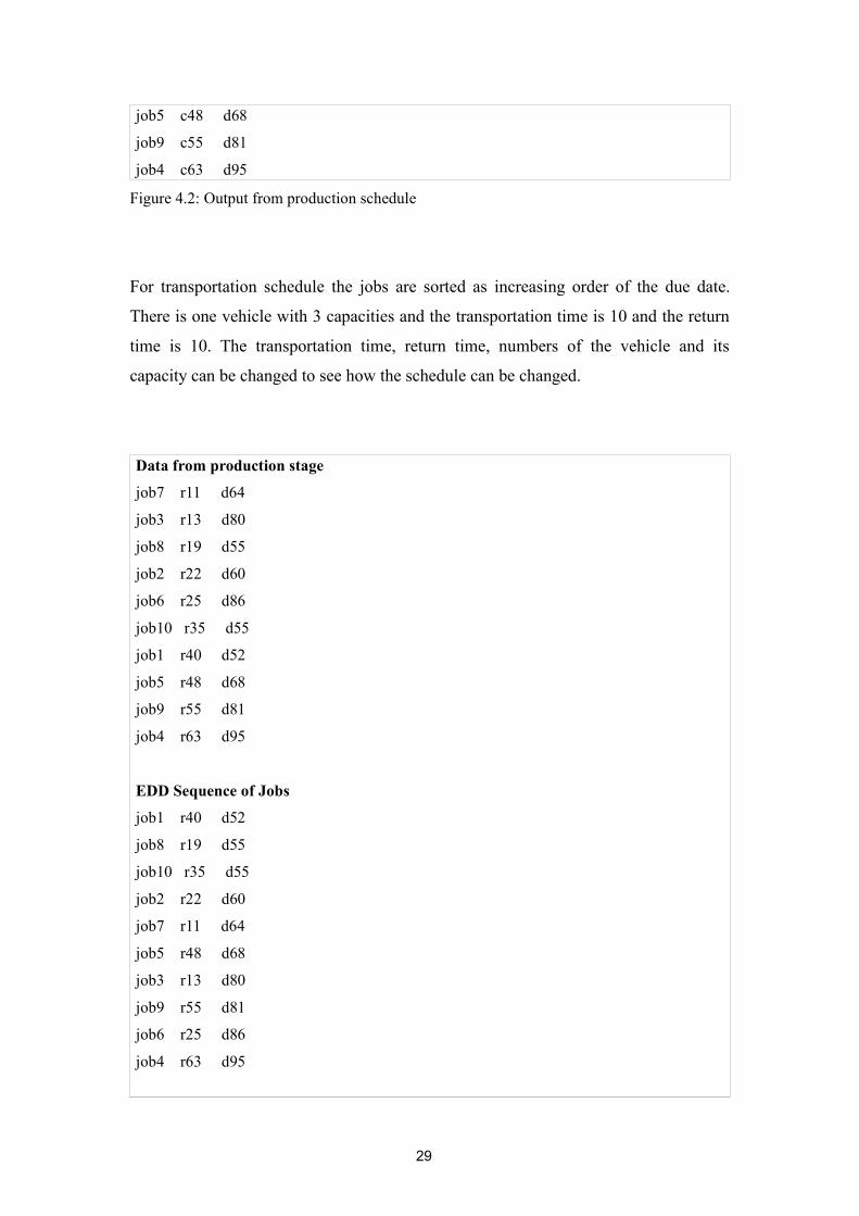
job4 c63 d95

Figure 4.2: Output from production schedule

For transportation schedule the jobs are sorted as increasing order of the due date.

There is one vehicle with 3 capacities and the transportation time is 10 and the return

time is 10. The transportation time, return time, numbers of the vehicle and its

capacity can be changed to see how the schedule can be changed.

Data from production stage

job7 r11 d64

job3 r13 d80

job8 r19 d55

job2 r22 d60

job6 r25 d86

job10 r35 d55

job1 r40 d52

job5 r48 d68

job9 r55 d81

job4 r63 d95

EDD Sequence of Jobs

job1 r40 d52

job8 r19 d55

job10 r35 d55

job2 r22 d60

job7 r11 d64

job5 r48 d68

job3 r13 d80

job9 r55 d81

job6 r25 d86

job4 r63 d95

29

Batching

(1, 8, 10|2, 7, 5|3, 9, 6|4)

Total Completion Time

job1 c50 d52 -2

job8 c50 d55 -5

job10 c50 d55 -5

job2 c70 d60 10

job7 c70 d64 6

job5 c70 d68 2

job3 c90 d80 10

job9 c90 d81 9

job6 c90 d86 4

job4 c110 d95 15

Lmax is 15.

Figure 4.3: Final Output

From the final output (Figure 4.3) the manufacturer can draw a Gantt chart to view the

scheduled visually.

4.2 Testing

The algorithms are implemented in C++ and are tested to debug the program. Numbers of

different jobs have been tested to see whether the result was giving the correct solution such

as completion time and maximum lateness by comparing the solution worked by hand.

30

Chapter5

Computational Experiments

The purpose of the computational experiments is to analyse the effectiveness of the produced

solution. Production and transportation heuristic algorithm solutions will be evaluated by

comparing the solution that Branch and Bound algorithm has produced using LiSA.

5.1 Introduction

If the transportation time is zero for both trips then the production and transportation

schedule problem reduces the problem into production schedule problem of 1|rj|Lmax which is

NP-hard.

It is unlikely that the optimal solution can be found by a fast algorithm that is in polynomial

time, unless P = NP. It means that if the task is to find the optimal solution, then an

enumerative algorithm such as branch and bound algorithm can solve the problem with small

n(say n=5) and can work for hours and even days if n is large such as n = 20.

If the manufacturer has one vehicle with capacity of one then the production and

transportation schedule problem reduces to F2|rj|max. As the jobs will be delivered one at a

time so the transportation schedule will have the same order as the production schedule this

can be seen as a flow shop problem. The processing time for machine 2 will be same since

the delivery time is constant. The problem can not be solved in polynomial time as it is NP-

31

hard problem.

To get sure that finding an optimal solution is a difficult task, some experiments are made to

solve two special cases using LiSA.

5.2 Algorithms Used

Different combined heuristic algorithms are tested to find the best combination.

Combination 1 - production heuristic 1 with transportation heuristic 1.




Also Branch and bound algorithm is used to analyse the effectiveness of the solution.

5.3 Results

The running time of the combination heuristic algorithm is measured by the compilation time.

5.3.1 Experiment 1

The first experiment is to investigate whether the solution is optimal solution or the algorithm

is fast, a computational experiment with one vehicle which has one capacity. So, 1|rj|Lmax

problem can be seen as F2|rj|Lmax. The problem has been tested with 5 different random

numbers with 10 jobs to evaluate the running time and the objective function minimizing

lateness.

Accuracy is calculated as below:

Lmax(Si) - Lmax(S*)

Lmax(S*)

If the accuracy is high that indicates that the solution is far from optimal solution. The

average of the accuracy is calculated to find the best combination of heuristic algorithms. The

results are rounded up to 2 decimal points.

32

　　

Combination 1 Branch and bound(LiSA)Lmax time taken Lmax time taken Accuracy

test 1 29 6 sec 12 3 sec 1.42 test 2 18 6 sec 5 5 sec 2.60 test 3 38 4 sec 15 2 sec 1.53 test 4 40 5 sec 11 3 sec 2.64 test 5 55 6 sec 13 4 sec 3.23

Average 2.28

Table 5: Computational results for combination 1

　　


test 1 21 6 sec 12 3 sec 0.75test 2 14 6 sec 5 5 sec 1.80 test 3 25 4 sec 15 2 sec 0.67 test 4 21 5 sec 11 3 sec 0.91 test 5 30 6 sec 13 4 sec 1.31

Average 1.09


　　



Average 3.87


　　



33

Average 1.09


From the table above it can be seen that heuristic algorithms takes longer to produce solution.

The reason is that the Brach and bound algorithm can find optimal solution in a reasonable

time if the numbers of jobs are small. Another reason is that the algorithm which are

implemented uses bubble sort which takes O(n2) time.

The most efficient combination of heuristics algorithms are combination 2 and combination

4. Combination heuristic 2 is applying earliest due date for both production and

transportation schedule. Combination heuristic algorithm 4 is applying earliest due date for

production and earliest release date for transportation. In this special case both combinations

are actually the same. As the production and transportation problems have been divided into

sub-problems both of them are related to each other. Therefore sorting the jobs for

transportation schedule in combination heuristic 4 have the same effect of sorting the jobs

earliest due date. Since the jobs are released from the production in non-decreasing order of

the due date. The result shows that the important issue in order to minimise the lateness is the

due date.

5.3.2 Experiment 2

Branch and bound algorithm has been tested to verify 1|rj|Lmax and F2|rj|Lmax problems are NP-

hard. From LiSA the complexity of the problems is stated as “the current solution is minimal

NP-hard in the strong sense.” It has been tested with 5 jobs, 10 jobs, 15 jobs and 20 jobs. The

results are shown in table 9.

No. Jobs B&B Heuristic algorithm5 jobs 3 sec 4 sec

10 jobs 7 sec 5 sec15 jobs 1 minute 12 sec 5 sec20 jobs 27 minutes 13 sec 6 sec

Table 9: Time complexity for 1|rj| Lmax problem

The entire schedule is guaranteed to be optimal because branch and bound is an exact

34

algorithm for finding an optimal solution to an NP-hard problem. Besides it is optimal

because it is terminated within reasonable time. Figure 5 shows that the running time

dramatically increases after 15 jobs.

Another experiment is F2|rj| Lmax problem with 5 jobs, 10 jobs, 15 jobs and 20 jobs (see Table

10).

No. Jobs time taken5 jobs 3 sec

10 jobs 3 sec15 jobs 1 hour 20 min20 jobs more than 1 day

Table 10: Time complexity for F2|rj| Lmax problem

For jobs less than 10 the solution was found quickly but as the jobs increases computational

time is rapidly increases. For 20 jobs the algorithm has been terminated after one day as it

was still searching the tree. The result can be either optimal or non-optimal since it is a

partial schedule and has not been able to compute all possible schedules.

5.3.3 Experiment 3

The final experiment is to observe the running time of the heuristic algorithm with 20 jobs,

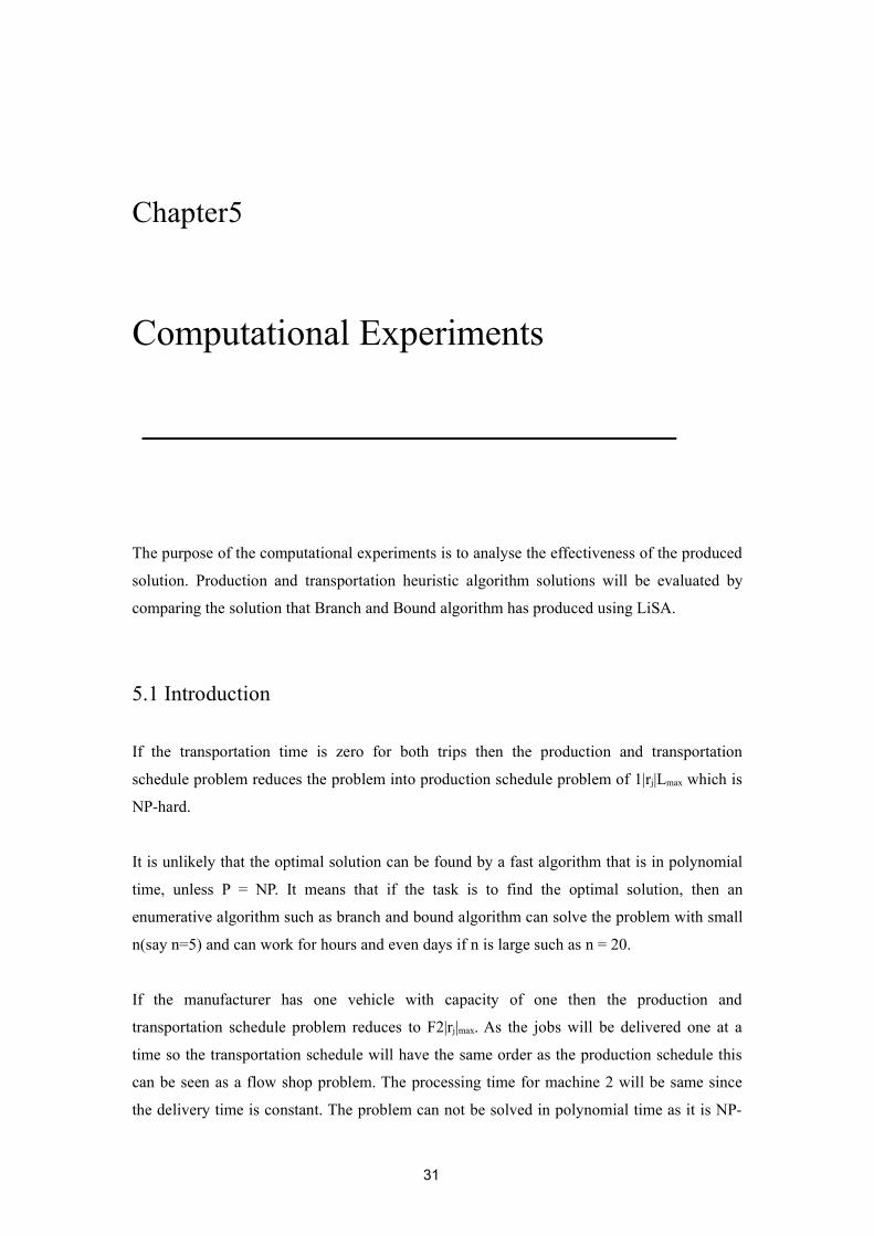
50 jobs, 100 jobs and 1000 jobs. Table 13 is the average of the running time of different

combination of heuristic algorithm.

No. Jobs time taken10 jobs 5 sec50 jobs 5 sec

100 jobs 6 sec1000 jobs 10 sec

Table 11: Average computational time for 1|rj|Lmax

35

Average computational time for 1| rj| Lmax

0

2

46

8

10

12

14

10 jobs 50 jobs 100 jobs 1000 jobs

com

puta

tion

time

Heurstic algorithm

Figure 5.1: Graph from table 11

It shows that even with large number of jobs such as 1000 jobs the algorithm is still fast as

the graph slowly increases.

36

Chapter6

Evaluations

6.1 Minimum requirements

The minimum requirements of the project mentioned have been achieved (see section 1.3)

and are reproduced here:

To describe the scheduling model that involves transportation

To design algorithms for scheduling production and transportation

To implement one algorithm in C++ for scheduling production and transportation

To perform computational experiments and to analyse the performance of the

algorithm

Not only are all of the minimum requirements achieved but also it has been exceeded by

performing two of possible enhancements. Those are designing of a local search algorithm

and implementing several additional heuristic algorithms.

6.2 Evaluation of the algorithms

The objective criteria are analysing computation time and the accuracy between heuristic

algorithms and exact algorithm.

37

6.2.1 Accuracy of the algorithm

Figure 6.1 has been produced from computational experiments to see how far the schedules

are from optimal (see 5.3.1). Lower the accuracy closer to optimal solution.

Accuracy of the Algorithms

012345678

test 1 test 2 test 3 test 4 test 5

accu

racy Combination 1

Combination 2Combination 3Combination 4

Figure 6.1: The accuracy of the combination algorithms

When designing the algorithm I assumed that the best combination is applying earliest release

date for production schedule and earliest due date for transportation schedule (see 3.3). But

the assumption has been proved wrong as figure 4 illustrates that the best combinations are

applying earliest due date for both production and transportation schedule(combination 2) or

combination of earliest due date for production and earliest release date for transportation

schedule(combination 4). Furthermore it can be derived that the assumption made in design

stage is the worst combination of all.

6.2.2 Computation time of the algorithm

Figure 6.2 and 6.3 are obtained from the computational experiments in chapter 5(see 5.3.2).

38

Computation time for 1| rj| Lmax problem

0200400600800

10001200140016001800


seco

nds

B&BHeuristic algorithm

Figure 6.2: Comparison of running time for 1|rj| Lmax problem

Computation time for F2| rj| Lmax problem

0200400600800

1000120014001600


min

utes

Branch and Bound

Figure 6.3: Computation time for F2|rj| Lmax problem

Both figures (Figure 6.2 and 6.3) obviously illustrates those more than 15 jobs the

computation time increases dramatically while heuristic algorithm hardly increases.

Below is the result obtained from 20 jobs for heuristic algorithm and branch and bound. The

results will be compared with each other.

39

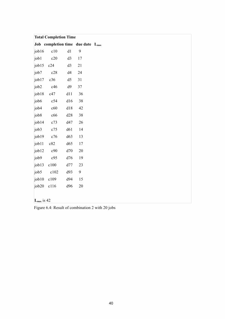
Total Completion Time

Job completion time due date Lmax

job16 c10 d1 9

job1 c20 d3 17

job15 c24 d3 21

job7 c28 d4 24

job17 c36 d5 31

job2 c46 d9 37

job18 c47 d11 36

job6 c54 d16 38

job4 c60 d18 42

job8 c66 d28 38

job14 c73 d47 26

job3 c75 d61 14

job19 c76 d63 13

job11 c82 d65 17

job12 c90 d70 20

job9 c95 d76 19

job13 c100 d77 23

job5 c102 d93 9

job10 c109 d94 15

job20 c116 d96 20

Lmax is 42

Figure 6.4: Result of combination 2 with 20 jobs

40

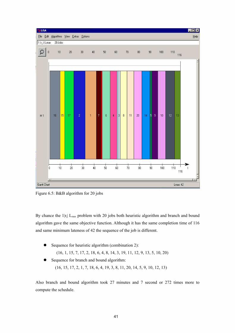
Figure 6.5: B&B algorithm for 20 jobs

By chance the 1|rj| Lmax problem with 20 jobs both heuristic algorithm and branch and bound

algorithm gave the same objective function. Although it has the same completion time of 116

and same minimum lateness of 42 the sequence of the job is different.

Sequence for heuristic algorithm (combination 2):

(16, 1, 15, 7, 17, 2, 18, 6, 4, 8, 14, 3, 19, 11, 12, 9, 13, 5, 10, 20)

Sequence for branch and bound algorithm:

(16, 15, 17, 2, 1, 7, 18, 6, 4, 19, 3, 8, 11, 20, 14, 5, 9, 10, 12, 13)

Also branch and bound algorithm took 27 minutes and 7 second or 272 times more to

compute the schedule.

41

6.3 Summary

Although production and transportation algorithm does not guarantee optimal solution but

nevertheless it will be preferable than exact algorithm if the jobs are large. It will be more

realistic as in real life the number of jobs to be schedules are tremendous. It will complement

for the weak points in the algorithm if local search method is used. Local search is discussed

in enhancement section (see 7.3.1).

42

Chapter7

Conclusions and Future Work

The last chapter summarizes the whole project and describe possible extensions which can be

done as future work.

7.1 Review of the Project

The overall ain of this project is to develop heuristic algorithms for integrated problems of

production and transportation schedule. The objective function was to minimize the

maximum lateness. The problem is strongly NP-hard. Some special cases have mentioned and

have been computational experimented for evaluation.

7.2 Conclusion

The transportation time is 0 for both trips then the production and transportation scheduling

problem reduces the problem into production schedule problem of one machine with the

objectives of minimizing maximum lateness taking release date into account. Another

problem is when the vehicle capacity is 1 the production and transportation scheduling

problem can be reduced as a flow shop problem where there is 2 machines with minimizing

maximum lateness as its objectives. Both solution can be produced in polynomial time but it

will not guarantee optimal solution.

43

It can be concluded that the simplified problem for production and transportations scheduling

in this report has been proved to be NP-hard.

7.3 Future Work

There are some possible enhancements listed below for future work. Developing different

heuristic algorithm can be thought as future work.

7.2.1 General Suggestions about local search

The local search method will improve to find better solution than heuristic algorithm.

Although it finds better solution it does not guarantee that it is an optimum solution. There

exists different method of local search. As mentioned earlier threshold accepting has been

chosen for local search method.

For step 1, the initial schedule is selected from the schedule which was obtained by applying

heuristic algorithms described above. The initial schedule will consist of production schedule

and transportation schedule which form a whole. M (sequence) is the permutation of n

numbers of the sequence for production schedule and T (sequence) is the permutation of n

numbers of the sequence for transportation schedule.

There are different methods of generating neighbours S’ for step 2. Three methods are

mentioned.

One of the methods is to transpose neighbour by swapping two adjacent jobs in the

production schedule or transportation schedule or even both.

e.g.) swapping two adjacent jobs which is indicated in bold for production schedule.

S= M(5,3,2,1,4), T(1,2|5,3,4)

→ F(S’) = M(3,5,2,1,4), T(1|2,5|3,4)

44

Another method is to swap neighbour by swapping two arbitrary jobs in the sequence. Also

one job can be moved to other position which is called insert neighbourhood. These methods

can be utilised to change the sequence of the jobs in transportation schedule.

e.g.) S= M(5,3,2,1,4), T(1,2|5,3,4)

→ S’= M(1,3,2,5,4), T(1|2,5|3,4)

Finally, because the schedule is divided into batch which is represented as deliminator (i.e. |)

can be moved to different place without violating the capacity of the vehicle. Below is an

example of this method.

e.g.) S= M(5,3,2,1,4), T(1,2|5,3,4)

→ S’ = M(5,3,2,1,4), T(1|2,5|3,4)

Neighbours can be generated randomly or systematically. Combination of two methods can

be considered as well so it will search possible neighbours to minimize the maximum

lateness.

The acceptance test is that if Lmax(S’) <Lmax(S) +α, where threshold value is greater than zero

i.e. α>0. Threshold value is generally starts with a large value and it gradually reduces later

on. For step 4, the algorithm will terminates if the fixed computational time exceeds or after

number of iterations.

Although this approach might cycle thought the schedule which has already been visited but

it has higher probability of finding better solution than schedule which merely applying

heuristic algorithm. It may find optimal solution however it can be local optimal solution.

Based on this local search for future work the algorithm can be written as a program so the

solution can be compared and the results can be evaluated.

7.3.3 Design of exact algorithms for the special cases of the problem

For special cases of the problem exact algorithms can be designed.

45

7.3.2 Generalising the heuristic algorithms for solving more complex problems

As the problem is generalised from production and transportation problem more complex

problem can be explored. From the definition of production and transportation scheduling

problem (see section 2.6.2) the problem can have several suppliers, manufacturer and several

customers with several transportation vehicles.

In addition to have more complex problem vehicle routing problem can be introduced.

46

Bibiliography

[1] Brucker P. Scheduling Algorithms. 3rd edition. London: Springer, 2001.

[2] Brucker P., Knust S., Complexity results for scheduling problems

URL: http://www.mathematik.uni-osnabrueck.de/research/OR/class/

[25th March 2005]

[3] Beasley J.E., Lucena A., Marcus Poggi de Arago, The Vehicle Routing Problem.

Handbook of Applied Optimization. Oxford University Press, 2002.

[4] Chang Y.C., Lee C.Y., Machine scheduling with job delivery coordination. European

Journal of Operational Research 158, pages 470-487, 2004.

[5] Deitel H.M, Deitel P.J, C++ How to Program. 3rd edition, Prentice Hall, 2001.

[6] Lee C.Y., Chen Z.L., Machine scheduling with transportation consideration. Journal of

Scheduling, 4:3-24, 2001.

[7] Pinedo M. Scheduling: Theory, Algorithms, and Systems. 2nd edition. New Jersey:

Prentice Hall, 2002.

[8] Shakhlevich N. OR32: Scheduling: Models and Algorithms Notes. University of Leeds,

2004.

[9] Wang C.S., Uzsoy R., A genetic algorithm to minimize maximum lateness on a batch

processing machine. Computers and Operations Research 29, 1621-1640, 2002.

47

Appendix A

This project was interesting as it gave me an opportunity to understand the production and

transportation problem a little deeply and produce a solution.

Time management is an important issue in project. The project schedule should be scheduled

realistically and evenly throughout the week. I believe that if the project was done with no

other work such as coursework for other modules the project could have dealt more widely

and deeply. It is advisable to next year students to take fewer modules in semester 2 so the

project can be done according to the schedule.

48

heuristic algorithms for solving problem that involves ... · pdf filethis chapter will...

Documents