heterodyne receivers - iram.es · pdf fileheterodyne receivers ... the main roles of a...
TRANSCRIPT

Heterodyne Receivers Introduction to heterodyne receivers for
cm and mm-wave radioastronomy
Alessandro Navarrini IRAM, Grenoble
September 27th, 2011
6th 30 m Summer School

Geometry of the IRAM 30 m telescope optics
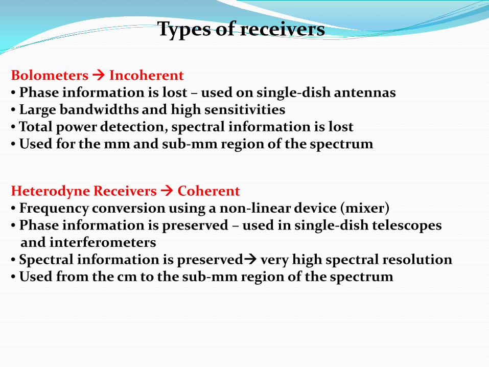
Heterodyne Receivers Coherent • Frequency conversion using a non-linear device (mixer) • Phase information is preserved – used in single-dish telescopes and interferometers • Spectral information is preserved very high spectral resolution • Used from the cm to the sub-mm region of the spectrum
Types of receivers
Bolometers Incoherent • Phase information is lost – used on single-dish antennas • Large bandwidths and high sensitivities • Total power detection, spectral information is lost • Used for the mm and sub-mm region of the spectrum
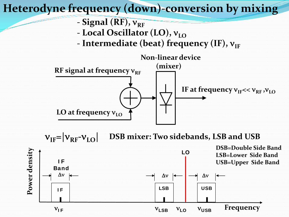
RF signal at frequency νRF
LO at frequency νLO
IF at frequency νIF<< νRF ,νLO
Non-linear device (mixer)
LSB
νLSB
∆ν
USB
νUSB
∆ν
IF
νIF
IF Band ∆ν
νLO
LO
νIF=|νRF-νLO| DSB mixer: Two sidebands, LSB and USB
Frequency
Pow
er d
ensi
ty
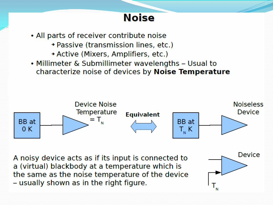
Heterodyne frequency (down)-conversion by mixing - Signal (RF), νRF - Local Oscillator (LO), νLO - Intermediate (beat) frequency (IF), νIF
DSB=Double Side Band LSB=Lower Side Band USB=Upper Side Band
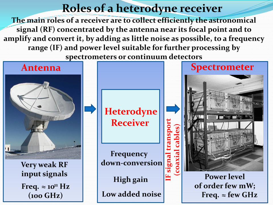
The main roles of a receiver are to collect efficiently the astronomical signal (RF) concentrated by the antenna near its focal point and to
amplify and convert it, by adding as little noise as possible, to a frequency range (IF) and power level suitable for further processing by
spectrometers or continuum detectors
Very weak RF input signals
Freq. ≈ 1011 Hz (100 GHz)
Power level of order few mW;
Freq. ≈ few GHz
High gain
Frequency down-conversion
Low added noise
Roles of a heterodyne receiver
IF s
igna
l tra
nspo
rt
(coa
xial
cab
les)
Antenna Spectrometer
Heterodyne Receiver

IRAM 30 m telescope receiver cabin

Active component technologies for heterodyne receivers
SIS mixers • Heterodyne mixing • 700GHz (Nb); >1THz (NbTiN) • Instantaeneous b/w 2 x 8 GHz
HEB mixers • Heterodyne mixing • Several THz • Instantaeneous b/w ~ 4 GHz
HEMT amplifiers • Direct amplification • 115 GHz on telescopes; beyond 200 GHz in the lab • Instantaneous b/w ~ 30%
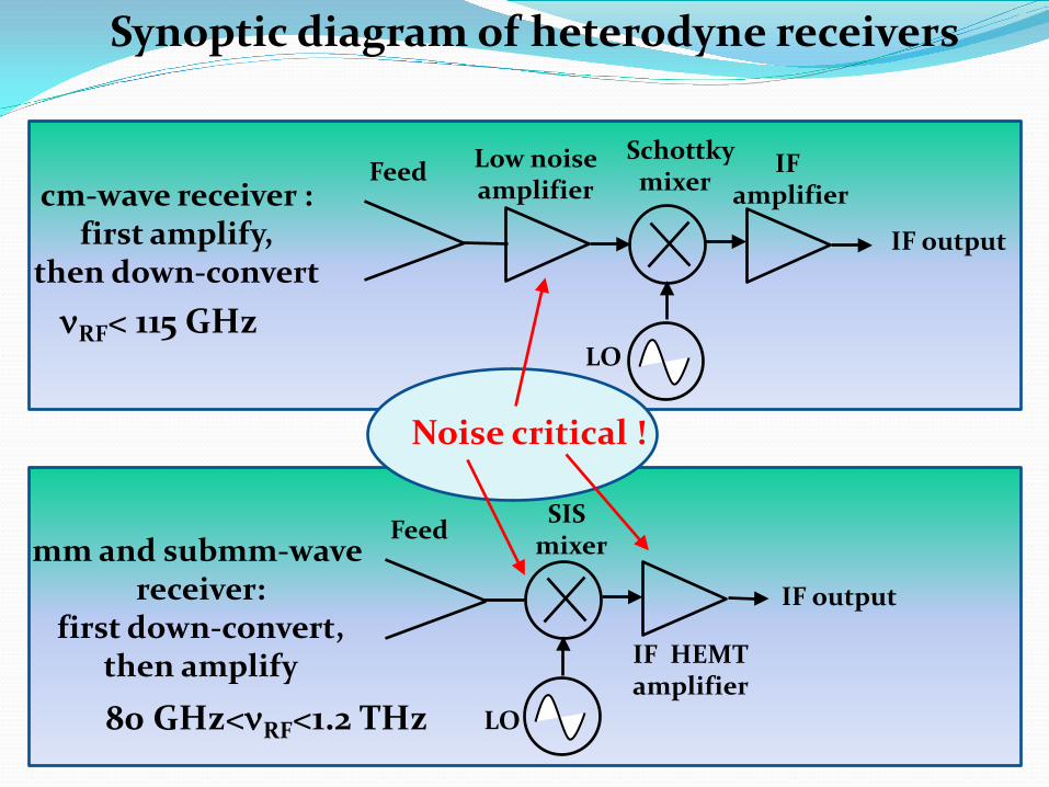
Synoptic diagram of heterodyne receivers
Schottky mixer
LO
IF output
Feed Low noise amplifier
IF amplifier cm-wave receiver :
first amplify, then down-convert
SIS mixer
LO
Feed
IF HEMT amplifier
mm and submm-wave receiver:
first down-convert, then amplify
IF output
80 GHz<νRF<1.2 THz
Noise critical !
νRF< 115 GHz

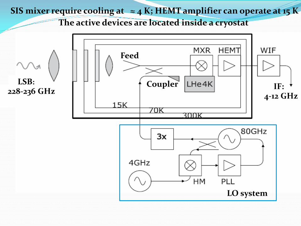
SIS mixer requires cooling at ≈ 4 K; HEMT amplifier can operate at 15 K.
LO system
4-12 GHz
228-236 GHz
LSB:
240 GHz
IF:
LO:
Feed
Coupler
The active devices are located inside a cryostat:
LO system
Feed
Coupler 4-12 GHz
228-236 GHz
LSB: IF:
SIS mixer require cooling at ≈ 4 K; HEMT amplifier can operate at 15 K The active devices are located inside a cryostat
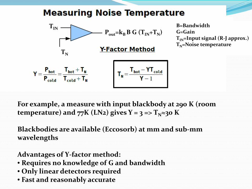
For example, a measure with input blackbody at 290 K (room temperature) and 77K (LN2) gives Y = 3 => TN≈30 K Blackbodies are available (Eccosorb) at mm and sub-mm wavelengths Advantages of Y-factor method: • Requires no knowledge of G and bandwidth • Only linear detectors required • Fast and reasonably accurate
Pout=kB B G (TIN+TN)
B=Bandwidth G=Gain TIN=Input signal (R-J approx.) TN=Noise temperature
TIN
TN
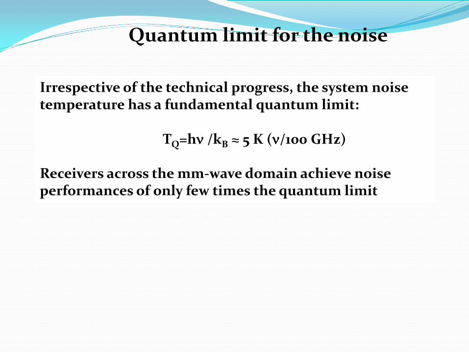
Irrespective of the technical progress, the system noise temperature has a fundamental quantum limit: TQ=hν /kB ≈ 5 K (ν/100 GHz) Receivers across the mm-wave domain achieve noise performances of only few times the quantum limit
Quantum limit for the noise

Noise temperature of a cascade of stages
• For a cascade of stages with gain Gi>>1, the noise of the first stage TN1 dominates the overall noise temperature.
Noise temperature of an attenuator
… with attenuation L and physical temperature Tphys: TN=Tphys(L-1) Cooling the low loss optics and the waveguide components (feed, OMT) in front of the active devices reduces the receiver noise temperature.
• If the first stage has loss (G1=1/L1<1) or little gain, the noise temperature of the subsequent stage can become important. This is the case of SIS mixers, whose gain is of order 1 or lower.

Corrugated feed-horn for the 2 mm band (129-174 GHz) of the 30 m telescope
A relay optics is typically used to image the horn aperture on the telescope’s aperture. This fulfils the condition of frequency-independent illumination.
A scalar, or conical corrugated feed-horn, generates an electric field with almost perfect Gaussian distribution at its aperture. 98% of the power radiated (or received) by the conical corrugated feed is in the fundamental Gaussian mode
C-band (5.7-7.7 GHz) feed-horn for the beam waveguide focus of SRT
Feed Horns
Physical dimensions scale ≈ with wavelength

HEMT low noise amplifiers (LNA)
MMIC
Discrete transistors
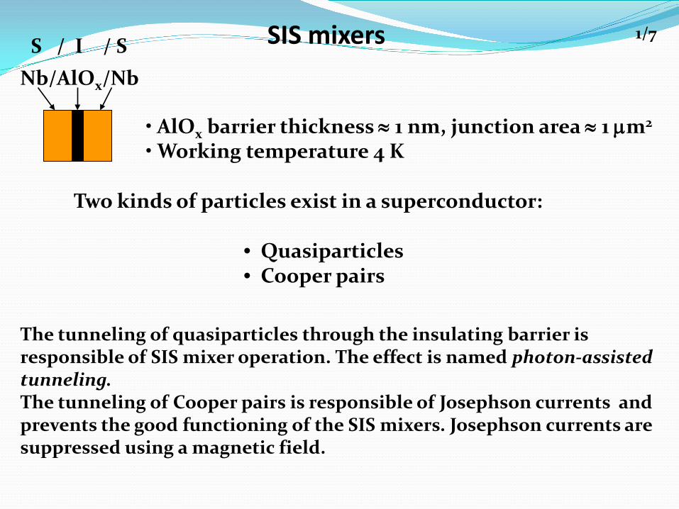
SIS mixers
Two kinds of particles exist in a superconductor:
• Quasiparticles • Cooper pairs
Nb/AlOx/Nb
• AlOx barrier thickness ≈ 1 nm, junction area ≈ 1 µm2 • Working temperature 4 K
The tunneling of quasiparticles through the insulating barrier is responsible of SIS mixer operation. The effect is named photon-assisted tunneling. The tunneling of Cooper pairs is responsible of Josephson currents and prevents the good functioning of the SIS mixers. Josephson currents are suppressed using a magnetic field.
1/7 S / I / S
0 1 2 3 4 5
0,00
0,05
0,10
0,15
0,20
0,25
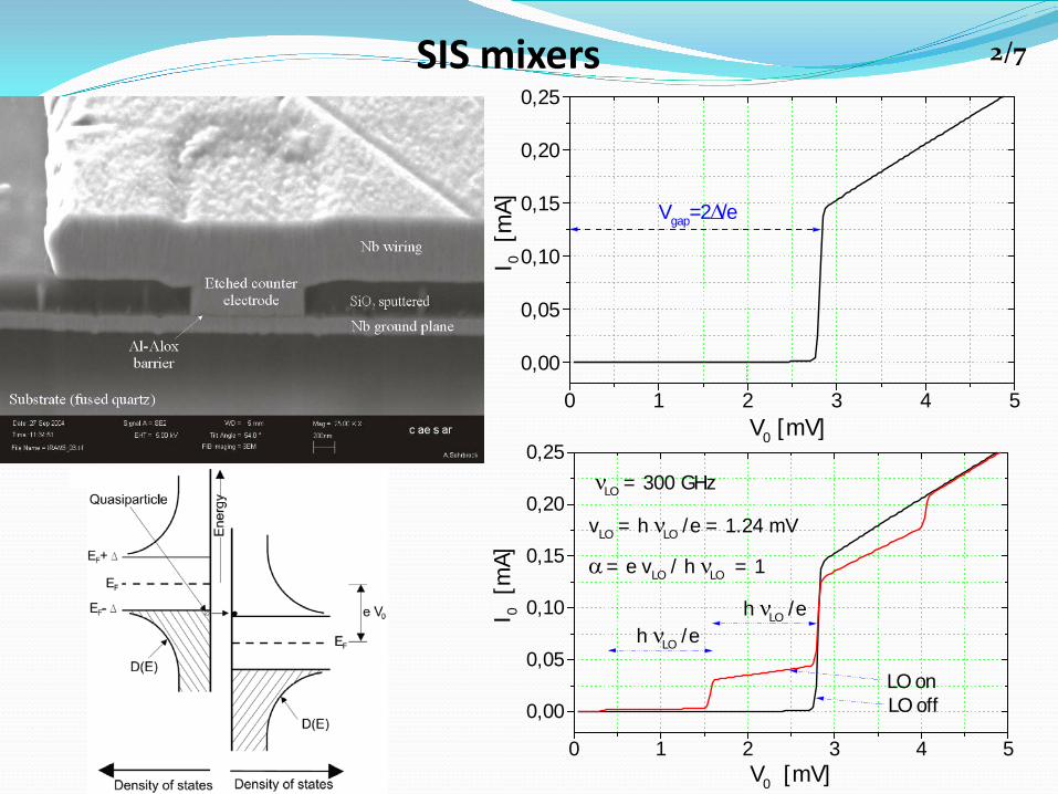
Vgap=2∆/e
I 0 [m
A]
V0 [mV]
2/7 SIS mixers
0 1 2 3 4 5
0,00
0,05
0,10
0,15
0,20
0,25
α = e vLO / h νLO = 1
LO offLO on
h νLO /eh νLO /e
vLO = h νLO /e = 1.24 mV
νLO = 300 GHz
I 0 [m
A]
V0 [mV]

ALMA Band 7 mixer chip 275-373 GHz
Waveguide SIS mixers 80-116 GHz mixer
• SIS junctions located on a quartz substrate • Waveguide probe couples the signal into the SIS junction(s), usually through microstrip and/or coplanar waveguides • Superconducting Nb transmission lines
3/7
SIS mixer types
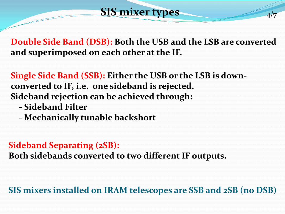
Double Side Band (DSB): Both the USB and the LSB are converted and superimposed on each other at the IF.
Single Side Band (SSB): Either the USB or the LSB is down-converted to IF, i.e. one sideband is rejected. Sideband rejection can be achieved through: - Sideband Filter - Mechanically tunable backshort
Sideband Separating (2SB): Both sidebands converted to two different IF outputs.
4/7
SIS mixers installed on IRAM telescopes are SSB and 2SB (no DSB)
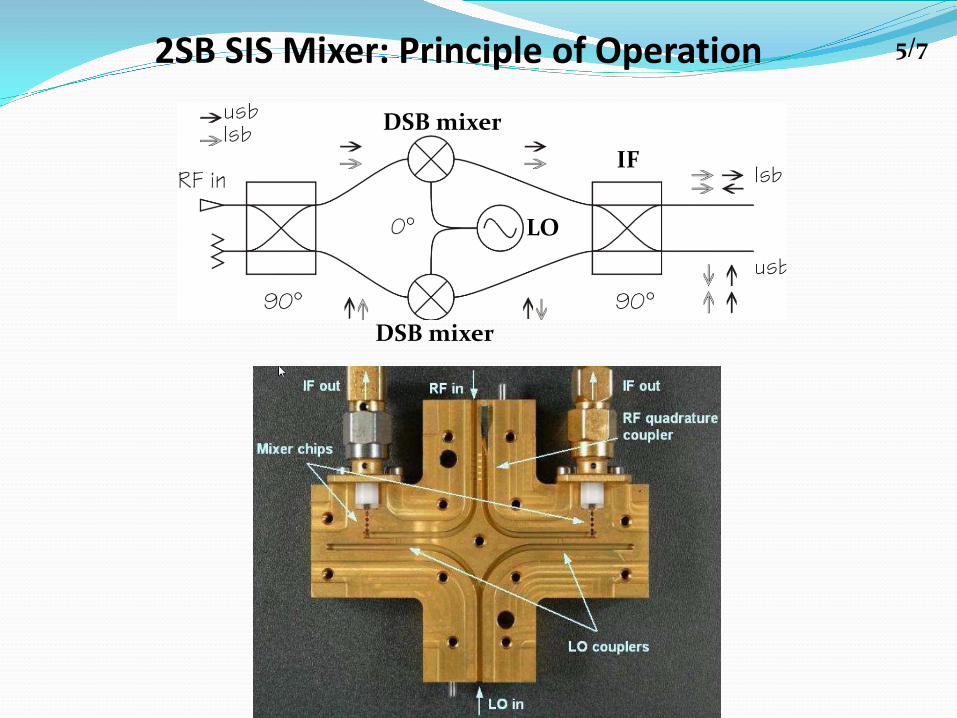
2SB SIS Mixer: Principle of Operation 5/7
LO
DSB mixer
DSB mixer
IF
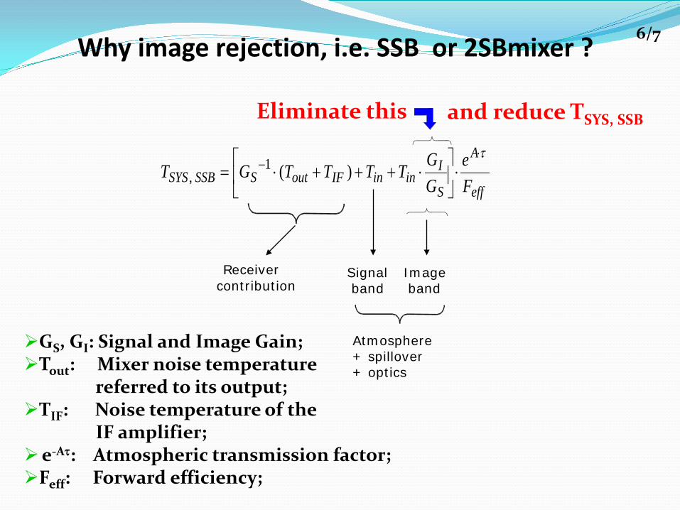
Why image rejection, i.e. SSB or 2SBmixer ?
eff
A
S
IininIFoutSSSBSYS F
eGGTTTTGT
τ⋅− ⋅
⋅+++⋅= )(1
,
Eliminate this and reduce TSYS, SSB
GS, GI: Signal and Image Gain; Tout: Mixer noise temperature referred to its output; TIF: Noise temperature of the IF amplifier; e-Aτ: Atmospheric transmission factor; Feff: Forward efficiency;
Atmosphere + spillover + optics
Receiver contribution
Signal band
Image band
6/7
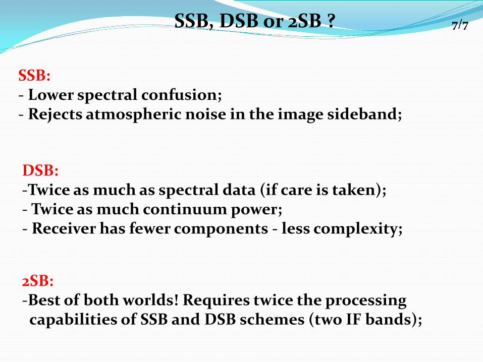
SSB, DSB or 2SB ?
SSB: - Lower spectral confusion; - Rejects atmospheric noise in the image sideband;
DSB: -Twice as much as spectral data (if care is taken); - Twice as much continuum power; - Receiver has fewer components - less complexity;
2SB: -Best of both worlds! Requires twice the processing capabilities of SSB and DSB schemes (two IF bands);
7/7
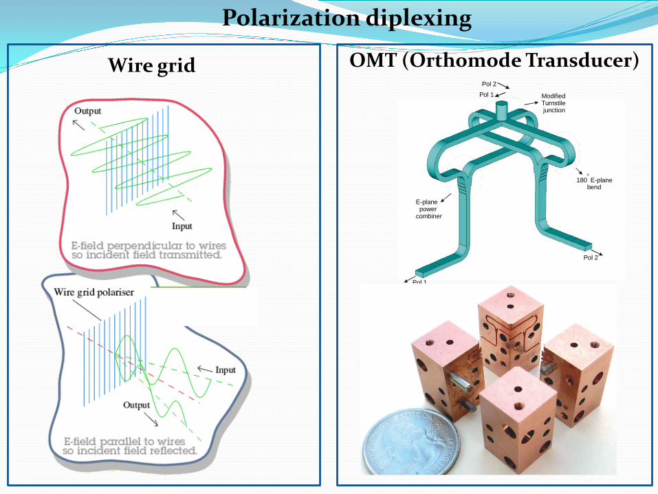
Wire grid
ModifiedTurnstile junction
180 E-plane bend
0
E-plane powercombiner
Pol 2Pol 1
Pol 1
Pol 2
Polarization diplexing
OMT (Orthomode Transducer)

Electromagnetic modeling softwares
• A number of powerful commercial electromagnetic softwares are available • They allow accurate modeling of 2D (planar circuitry) and 3D (waveguide and antenna structures). Fast computers are required to perform optimizations on a large parameter space
• Mechanical modeling CADs have also a primary importance for the receiver designer

EMIR: Multi-band mm-wave SIS receiver for IRAM 30 m telescope 1/4
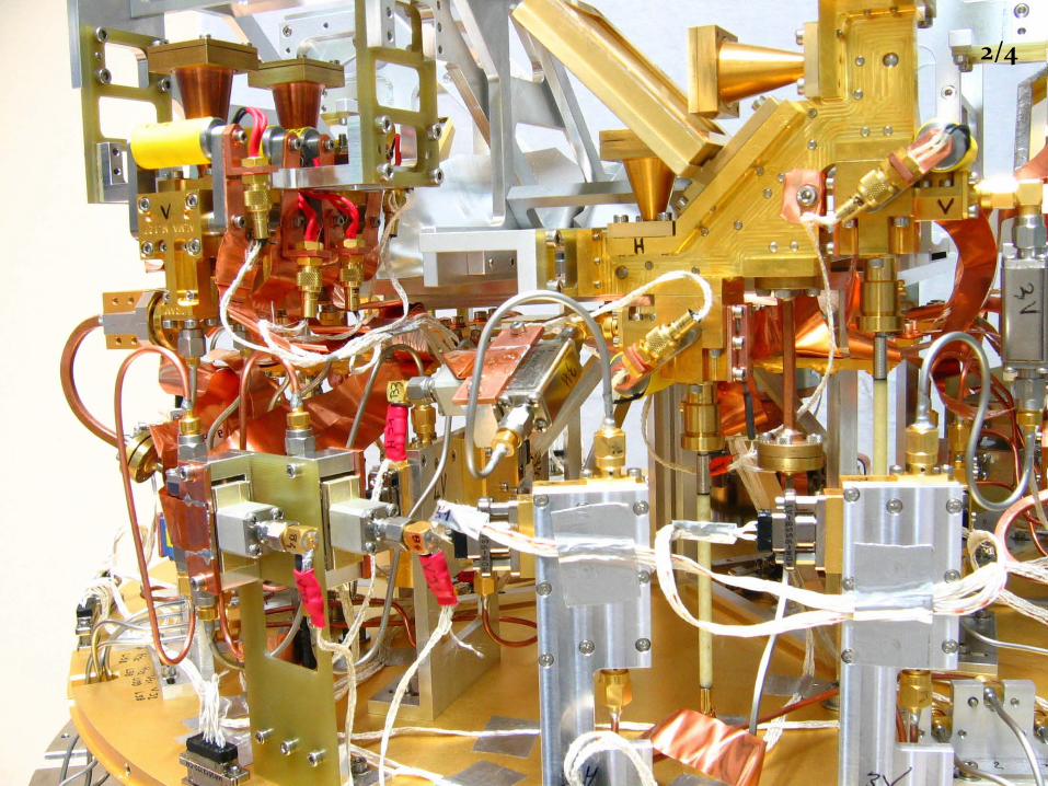
2/4

EMIR Band 3 (200-267 GHz) cold optics module 3/4

Receiver performance in the four EMIR RF bands 4/4
Typical receiver requirements
• Receiver technology: HEMT, SIS (DSB, SSB or 2SB)
• Stability: total power stability expressed as Allan deviation • Linearity
• Polarization purity
• Freedom from spurious response (suppression of image sideband)
• Multiband operation (observe two RF bands simultaneously, frequency diplexing) • Dual-polarization (linear or circular) with OMTs or quasi-optics wire grids.
• Sensitivity: receiver and system noise temperatures referred to the input; cal. load
• RF band (typically ΔνRF/νRF ≈ 30-40%) • IF band: (ΔνIF/νRF ≈15% for SIS, ≈30% for HEMT)
• Full remote control of all functions (bias, temperatures, etc.)
• No cryogenic fluid refills: closed cycle cryocooler
• Optimum optical coupling to the antenna
• Power level (in dBm/MHz) at the IF receiver output
• Screened from external RFI environment and free from self-generating RFI
• IF passband flatness (minimum slope and ripple)
• LO tuning range (from RF and IF) and LO type (Gunn, YIG+AMC, photonic, or QCL)
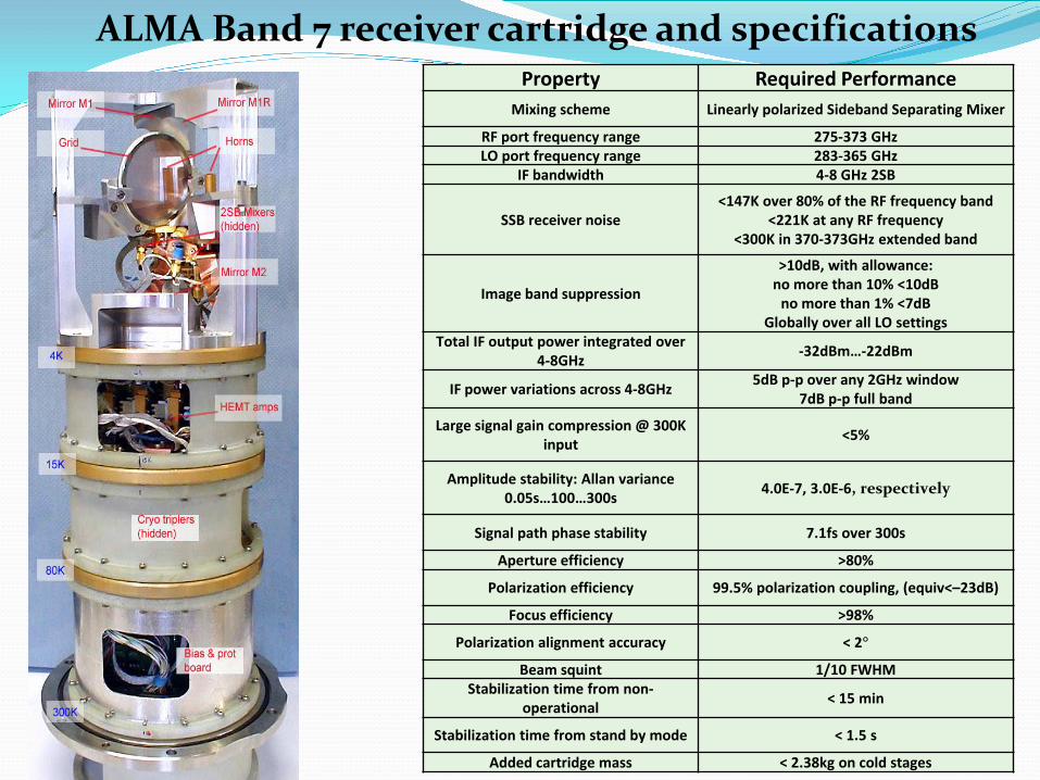
Property Required Performance Mixing scheme Linearly polarized Sideband Separating Mixer
RF port frequency range 275-373 GHz LO port frequency range 283-365 GHz
IF bandwidth 4-8 GHz 2SB
SSB receiver noise <147K over 80% of the RF frequency band
<221K at any RF frequency <300K in 370-373GHz extended band
Image band suppression
>10dB, with allowance: no more than 10% <10dB
no more than 1% <7dB Globally over all LO settings
Total IF output power integrated over 4-8GHz
-32dBm…-22dBm
IF power variations across 4-8GHz 5dB p-p over any 2GHz window
7dB p-p full band
Large signal gain compression @ 300K input
<5%
Amplitude stability: Allan variance 0.05s…100…300s
4.0E-7, 3.0E-6, respectively
Signal path phase stability 7.1fs over 300s
Aperture efficiency >80%
Polarization efficiency 99.5% polarization coupling, (equiv<–23dB)
Focus efficiency >98%
Polarization alignment accuracy < 2°
Beam squint 1/10 FWHM Stabilization time from non-
operational < 15 min
Stabilization time from stand by mode < 1.5 s
Added cartridge mass < 2.38kg on cold stages
ALMA Band 7 receiver cartridge and specifications

TQ=4hν /kB

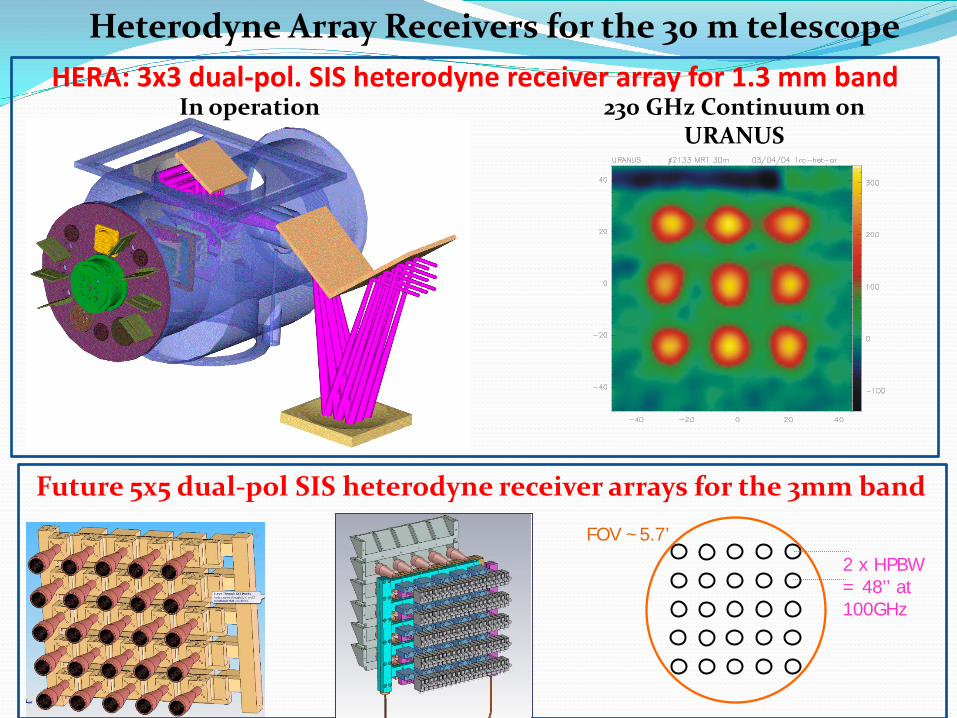
HERA: 3x3 dual-pol. SIS heterodyne receiver array for 1.3 mm band In operation
Heterodyne Array Receivers for the 30 m telescope
230 GHz Continuum on URANUS
Future 5x5 dual-pol SIS heterodyne receiver arrays for the 3mm band
2 x HPBW = 48’’ at 100GHz
FOV ~5.7’
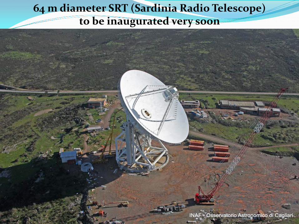
64 m diameter SRT (Sardinia Radio Telescope) to be inaugurated very soon
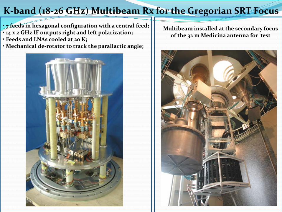
K-band (18-26 GHz) Multibeam Rx for the Gregorian SRT Focus
Multibeam installed at the secondary focus of the 32 m Medicina antenna for test
• 7 feeds in hexagonal configuration with a central feed; • 14 x 2 GHz IF outputs right and left polarization; • Feeds and LNAs cooled at 20 K; • Mechanical de-rotator to track the parallactic angle;
Thanks for your attention