Heritage and early history of the boundary element method

Alexander H.-D. Chenga,*, Daisy T. Chengb

aDepartment of Civil Engineering University of Mississippi, University, MS, 38677, USAbJohn D. Williams Library, University of Mississippi, University, MS 38677, USA

Received 10 December 2003; revised 7 December 2004; accepted 8 December 2004

Available online 12 February 2005

Abstract

This article explores the rich heritage of the boundary element method (BEM) by examining its mathematical foundation from the

potential theory, boundary value problems, Green’s functions, Green’s identities, to Fredholm integral equations. The 18th to 20th century

mathematicians, whose contributions were key to the theoretical development, are honored with short biographies. The origin of the

numerical implementation of boundary integral equations can be traced to the 1960s, when the electronic computers had become available.

The full emergence of the numerical technique known as the boundary element method occurred in the late 1970s. This article reviews the

early history of the boundary element method up to the late 1970s.

q 2005 Elsevier Ltd. All rights reserved.

Keywords: Boundary element method; Green’s functions; Green’s identities; Boundary integral equation method; Integral equation; History

1. Introduction

After three decades of development, the boundary

element method (BEM) has found a firm footing in the

arena of numerical methods for partial differential

equations. Comparing to the more popular numerical

methods, such as the Finite Element Method (FEM) and

the Finite Difference Method (FDM), which can be

classified as the domain methods, the BEM distinguish

itself as a boundary method, meaning that the numerical

discretization is conducted at reduced spatial dimension. For

example, for problems in three spatial dimensions, the

discretization is performed on the bounding surface only;

and in two spatial dimensions, the discretization is on the

boundary contour only. This reduced dimension leads to

smaller linear systems, less computer memory require-

ments, and more efficient computation. This effect is most

pronounced when the domain is unbounded. Unbounded

domain needs to be truncated and approximated in domain

methods. The BEM, on the other hand, automatically

models the behavior at infinity without the need of

deploying a mesh to approximate it. In the modern day

0955-7997/$ - see front matter q 2005 Elsevier Ltd. All rights reserved.

doi:10.1016/j.enganabound.2004.12.001

* Corresponding author. Tel.: C1 662 915 5362; fax: C1 662 915 5523.

E-mail address: acheng@olemiss.edu (A.H.-D. Cheng).

industrial settings, mesh preparation is the most labor

intensive and the most costly portion in numerical

modeling, particularly for the FEM [9] Without the need

of dealing with the interior mesh, the BEM is more cost

effective in mesh preparation. For problems involving

moving boundaries, the adjustment of the mesh is much

easier with the BEM; hence it is again the preferred tool.

With these advantages, the BEM is indeed an essential part

in the repertoire of the modern day computational tools.

In order to gain an objective assessment of the success of

the BEM, as compared to other numerical methods, a search

is conducted using the Web of ScienceSM, an online

bibliographic database. Based on the keyword search, the

total number of journal publications found in the Science

Citation Index Expanded 195 was compiled for several

numerical methods. The detail of the search technique is

described in Appendix. The result, as summarized in

Table 1, clearly indicates that the finite element method

(FEM) is the most popular with more than 66,000 entries.

The finite difference method (FDM) is a distant second with

more than 19,000 entries, less than one third of the FEM.

The BEM ranks third with more than 10,000 entries, more

than one half of the FDM. All other methods, such as the

finite volume method (FVM) and the collocation method

(CM), trail far behind. Based on this bibliographic search,

Engineering Analysis with Boundary Elements 29 (2005) 268–302

www.elsevier.com/locate/enganabound

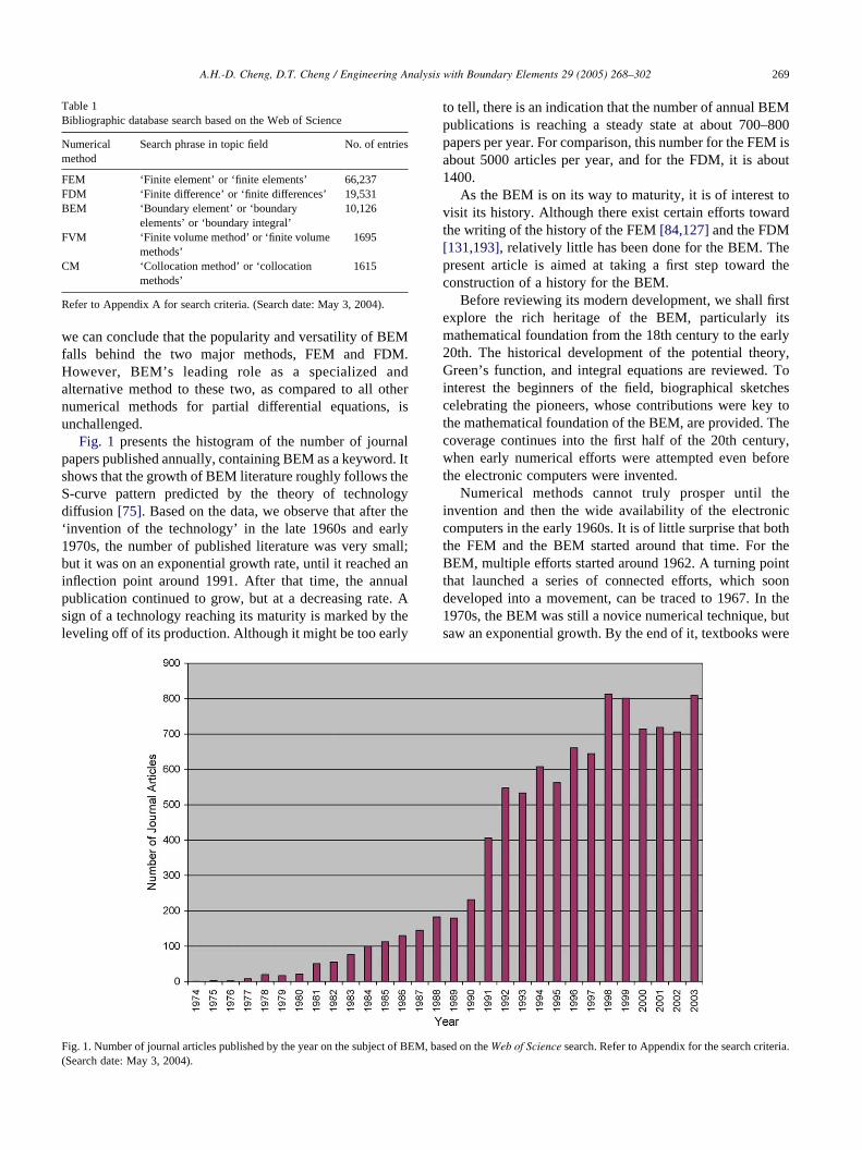
Table 1

Bibliographic database search based on the Web of Science

Numerical

method

Search phrase in topic field No. of entries

FEM ‘Finite element’ or ‘finite elements’ 66,237

FDM ‘Finite difference’ or ‘finite differences’ 19,531

BEM ‘Boundary element’ or ‘boundary

elements’ or ‘boundary integral’

10,126

FVM ‘Finite volume method’ or ‘finite volume

methods’

1695

CM ‘Collocation method’ or ‘collocation

methods’

1615

Refer to Appendix A for search criteria. (Search date: May 3, 2004).

A.H.-D. Cheng, D.T. Cheng / Engineering Analysis with Boundary Elements 29 (2005) 268–302 269

we can conclude that the popularity and versatility of BEM

falls behind the two major methods, FEM and FDM.

However, BEM’s leading role as a specialized and

alternative method to these two, as compared to all other

numerical methods for partial differential equations, is

unchallenged.

Fig. 1 presents the histogram of the number of journal

papers published annually, containing BEM as a keyword. It

shows that the growth of BEM literature roughly follows the

S-curve pattern predicted by the theory of technology

diffusion [75]. Based on the data, we observe that after the

‘invention of the technology’ in the late 1960s and early

1970s, the number of published literature was very small;

but it was on an exponential growth rate, until it reached an

inflection point around 1991. After that time, the annual

publication continued to grow, but at a decreasing rate. A

sign of a technology reaching its maturity is marked by the

leveling off of its production. Although it might be too early

Fig. 1. Number of journal articles published by the year on the subject of BEM, ba

(Search date: May 3, 2004).

to tell, there is an indication that the number of annual BEM

publications is reaching a steady state at about 700–800

papers per year. For comparison, this number for the FEM is

about 5000 articles per year, and for the FDM, it is about

1400.

As the BEM is on its way to maturity, it is of interest to

visit its history. Although there exist certain efforts toward

the writing of the history of the FEM [84,127] and the FDM

[131,193], relatively little has been done for the BEM. The

present article is aimed at taking a first step toward the

construction of a history for the BEM.

Before reviewing its modern development, we shall first

explore the rich heritage of the BEM, particularly its

mathematical foundation from the 18th century to the early

20th. The historical development of the potential theory,

Green’s function, and integral equations are reviewed. To

interest the beginners of the field, biographical sketches

celebrating the pioneers, whose contributions were key to

the mathematical foundation of the BEM, are provided. The

coverage continues into the first half of the 20th century,

when early numerical efforts were attempted even before

the electronic computers were invented.

Numerical methods cannot truly prosper until the

invention and then the wide availability of the electronic

computers in the early 1960s. It is of little surprise that both

the FEM and the BEM started around that time. For the

BEM, multiple efforts started around 1962. A turning point

that launched a series of connected efforts, which soon

developed into a movement, can be traced to 1967. In the

1970s, the BEM was still a novice numerical technique, but

saw an exponential growth. By the end of it, textbooks were

sed on the Web of Science search. Refer to Appendix for the search criteria.

A.H.-D. Cheng, D.T. Cheng / Engineering Analysis with Boundary Elements 29 (2005) 268–302270

written and conferences were organized on BEM. This

article reviews the early development up to the late 1970s,

leaving the latter development to future writers.

Before starting, we should clarify the use of the term

‘boundary element method’ in this article. In the narrowest

view, one can argue that BEM refers to the numerical

technique based on the method of weighted residuals,

mirroring the finite element formulation, except that the

weighing function used is the fundamental solution of

governing equation in order to eliminate the need of domain

discretization [19,21]. Or, one can view BEM as the

numerical implementation of boundary integral equations

based on Green’s formula, in which the piecewise element

concept of the FEM is utilized for the discretization [108].

Even more broadly, BEM has been used as a generic term

for a variety of numerical methods that use a boundary or

boundary-like discretization. These can include the general

numerical implementation of boundary integral equations,

known as the boundary integral equation method (BIEM)

[54], whether elements are used in the discretization or not;

or the method known as the indirect method that distributes

singular solutions on the solution boundary; or the method

of fundamental solutions in which the fundamental solutions

are distributed outside the domain in discrete or continuous

fashion with or without integral equation formulation; or

even the Trefftz method which distribute non-singular

solutions. These generic adoptions of the term are evident in

the many articles appearing in the journal of Engineering

Analysis with Boundary Elements and many contributions in

the Boundary Element Method conferences. In fact, the

theoretical developments of these methods are often

intertwined. Hence, for the purpose of the current historical

review, we take the broader view and consider into this

category all numerical methods for partial differential

equations in which a reduction in mesh dimension from a

domain-type to a boundary-type is accomplished. More

properly, these methods can be referred to as ‘boundary

methods’ or ‘mesh reduction methods.’ But we shall yield to

the popular adoption of the term ‘boundary element method’

for its wide recognition. It will be used interchangeably with

the above terms.

2. Potential theory

The Laplace equation is one of the most widely used

partial differential equations for modeling science and

engineering problems. It typically comes from the physical

consequence of combining a phenomenological gradient

law (such as the Fourier law in heat conduction and the

Darcy law in groundwater flow) with a conservation law

(such as the heat energy conservation and the mass

conservation of an incompressible material). For example,

Fourier law was presented by Jean Baptiste Joseph Fourier

(1768–1830) in 1822 [66]. It states that the heat flux in a

thermal conducting medium is proportional to the spatial

gradient of temperature distribution

q ZKkVT (1)

where q is the heat flux vector, k is the thermal conductivity,

and T is the temperature. The steady state heat energy

conservation requires that at any point in space the

divergence of the flux equals to zero:

V$q Z 0 (2)

Combining (1) and (2) and assuming that k is a constant, we

obtain the Laplace equation

V2T Z 0 (3)

For groundwater flow, similar procedure produces

V2h Z 0 (4)

where h is the piezometric head. It is of interest to mention

that the notation V used in the above came form William

Rowan Hamilton (1805–1865). The symbol V, known as

‘nabla’, is a Hebrew stringed instrument that has a triangular

shape [73].

The above theories are based on physical quantities. A

second way that the Laplace equation arises is through the

mathematical concept of finding a ‘potential’ that has no

direct physical meaning. In fluid mechanics, the velocity of

an incompressible fluid flow satisfies the divergence

equation

V$v Z 0 (5)

which is again based on the mass conservation principle. For

an inviscid fluid flow that is irrotational, its curl is equal to

zero:

V!v Z 0 (6)

It can be shown mathematically that the identity (6)

guarantees the existence of a scalar potential f such that

v Z Vf (7)

Combining (5) and (7) we again obtain the Laplace equation.

We notice that f, called the velocity potential, is a mathe-

matical conceptual construction; it is not associated with any

measurable physical quantity. In fact, the phrase ‘potential

function’ was coined by George Green (1793–1841) in his

1828 study [81] of electrostatics and magnetics: electric and

magnetic potentials were used as convenient tools for

manipulating the solution of electric and magnetic forces.

The original derivation of Laplace equation, however,

was based on the study of gravitational attraction, following

the third law of motion of Isaac Newton (1643–1727)

F ZKGm1m2r

jrj3(8)

where F is the force field, G is the gravitational constant, m1

and m2 are two concentrated masses, and r is the distance

vector between the two masses. Joseph-Louis Lagrange

A.H.-D. Cheng, D.T. Cheng / Engineering Analysis with Boundary Elements 29 (2005) 268–302 271

(1736–1813) in 1773 was the first to recognize the existence

of a potential function that satisfied the above equation [111]

f Z1

r(9)

whose spatial gradient gave the gravity force field

F Z Gm1m2Vf (10)

Subsequently, Pierre-Simon Laplace (1749–1827) in his

study of celestial mechanics demonstrated that the gravity

potential satisfies the Laplace equation. The equation was

first presented in polar coordinates in 1782, and then in the

Cartesian form in 1787 as [109]:

v2f

vx2C

v2f

vy2C

v2f

vz2Z 0 (11)

The Laplace equation, however, had been used earlier in the

context of hydrodynamics by Leonhard Euler (1707–1783)

in 1755 [63], and by Lagrange in 1760 [110]. But Laplace

was credited for making it a standard part of mathematical

physics [15,100]. We note that the gravity potential (9)

satisfying (11) represents a concentrated mass. Hence it is a

‘fundamental solution’ of the Laplace equation.

Simeon-Denis Poisson (1781–1840) derived in 1813

[132] the equation of force potential for points interior to a

body with mass density r as

V2f ZK4pr (12)

This is known as the Poisson equation.

2.1. Euler

Leonhard Euler (1707–1783) was the son of a Lutheran

pastor who lived near Basel, Switzerland. While studying

theology at the University of Basel, Euler was attracted to

mathematics by the leading mathematician at the time,

Johann Bernoulli (1667–1748), and his two mathematician

sons, Nicolaus (1695–1726) and Daniel (1700–1782). With

no opportunity in finding a position in Switzerland due to his

young age, Euler followed Nicolaus and Daniel to Russia.

Later, at the age of 26, he succeeded Daniel as the chief

mathematician of the Academy of St Petersburg. Euler

surprised the Russian mathematicians by computing in 3

days some astronomical tables whose construction was

expected to take several months.

In 1741 Euler accepted the invitation of Frederick the

Great to direct the mathematical division of the Berlin

Academy, where he stayed for 25 years. The relation with

the King, however, deteriorated toward the end of his stay;

hence Euler returned to St Petersburg in 1766. Euler soon

became totally blind after returning to Russia. By dictation,

he published nearly half of all his papers in the last 17 years

of his life. In his words, ‘Now I will have less distraction’.

Without doubt, Euler was the most prolific and versatile

scientific writer of all times. During his lifetime, he

published more than 700 books and papers, and it took

St Petersburg’s Academy the next 47 years to publish the

manuscripts he left behind [31]. The modern effort of

publishing Euler’s collected works, the Opera Omnia [64]

begun in 1911. However, after 73 volumes and 25,000

pages, the work is unfinished to the present day.

Euler contributed to many branches of mathematics,

mechanics, and physics, including algebra, trigonometry,

analytical geometry, calculus, complex variables, number

theory, combinatorics, hydrodynamics, and elasticity. He

was the one who set mathematics into the modern notations.

We owe Euler the notations of ‘e’ for the base of natural

logs, ‘p’ for pi, ‘i’ forffiffiffiffiffiffiK1

p, ‘P

’ for summation, and the

concept of functions.

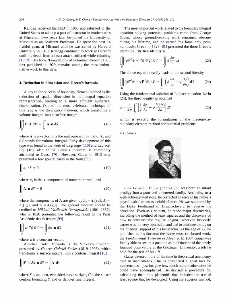
Carl Friedrich Gauss (1777–1855) has been called the

greatest mathematician in modern mathematics for his

setting up the rigorous foundation for mathematics. Euler,

on the other hand, was more intuitive and has been criticized

by pure mathematicians as being lacking rigor. However, by

the number indelible marks that Euler left in many science

and engineering fields, he certainly earned the title of the

greatest applied mathematician ever lived [58].

2.2. Lagrange

Joseph-Louis Lagrange (1736–1813), Italian by birth,

German by adoption, and French by choice, was next to

Euler the foremost mathematician of the 18th century. At

age 18 he was appointed Professor of Geometry at the Royal

Artillery School in Turin. Euler was impressed by his work,

and arranged a prestigious position for him in Prussia.

Despite the inferior condition in Turin, Lagrange only

wanted to be able to devote his time to mathematics; hence

declined the offer. However, in 1766, when Euler left Berlin

for St Petersburg, Frederick the Great arranged for Lagrange

to fill the vacated post. Accompanying the invitation was a

modest message saying, ‘It is necessary that the greatest

A.H.-D. Cheng, D.T. Cheng / Engineering Analysis with Boundary Elements 29 (2005) 268–302272

geometer of Europe should live near the greatest of Kings.’

To D’Alembert, who recommended Lagrange, the king

wrote, ‘To your care and recommendation am I indebted for

having replaced a half-blind mathematician with a

mathematician with both eyes, which will especially please

the anatomical members of my academy.’

After the death of Frederick, the situation in Prussia became

unpleasant for Lagrange. He left Berlin in 1787 to become a

member of the Academie des Sciences in Paris, where he

remained for the rest of his career. Lagrange’s contributions

were mostly in the theoretical branch of mathematics. In 1788

he published the monumental work Mecanique Analytique

that unified the knowledge of mechanics up to that time. He

banished the geometric idea and introduced differential

equations. In the preface, he proudly announced: ‘One will

not find figures in this work. The methods that I expound

require neither constructions, nor geometrical or mechanical

arguments, but only algebraic operations, subject to a regular

and uniform course.’ [31,128].

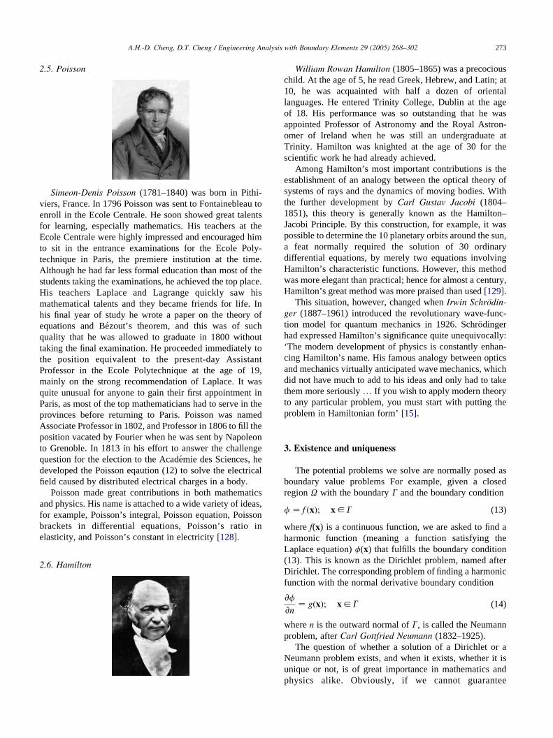
2.3. Laplace

Pierre-Simon Laplace (1749–1827), born in Normandy,

France, came from relatively humble origins. But with the

help of Jean le Rond D’Alembert (1717–1783), he was

appointed Professor of Mathematics at the Paris Ecole

Militaire when he was only 20-year old. Some years later, as

examiner of the scholars of the royal artillery corps, Laplace

happened to examine a 16-year old sub-lieutenant named

Napoleon Bonaparte. Fortunately for both of their careers, the

examinee passed. When Napoleon came to power, Laplace

was rewarded: he was appointed the Minister of Interior for a

short period of time, and later the President of the Senate.

Among Laplace’s greatest achievement was the five-

volume Traite du Mecanique Celeste that incorporated all

the important discoveries of planetary system of the

previous century, deduced from Newton’s law of gravita-

tion. Upon presenting the monumental work to Napoleon,

the emperor teasingly chided Laplace for an apparent

oversight: ‘They told me that you have written this huge

book on the system of the universe without once mentioning

its Creator’. Whereupon Laplace drew himself up and

bluntly replied, ‘I have no need for that hypothesis.’ [31].

He was eulogized by his disciple Poisson as ‘the Newton of

France’ [86]. Among the important contributions of Laplace in

mathematics and physics included probability, Laplace

transform, celestial mechanics, the velocity of sound, and

capillary action. He was considered more than anyone else to

have set the foundation of the probability theory [76].

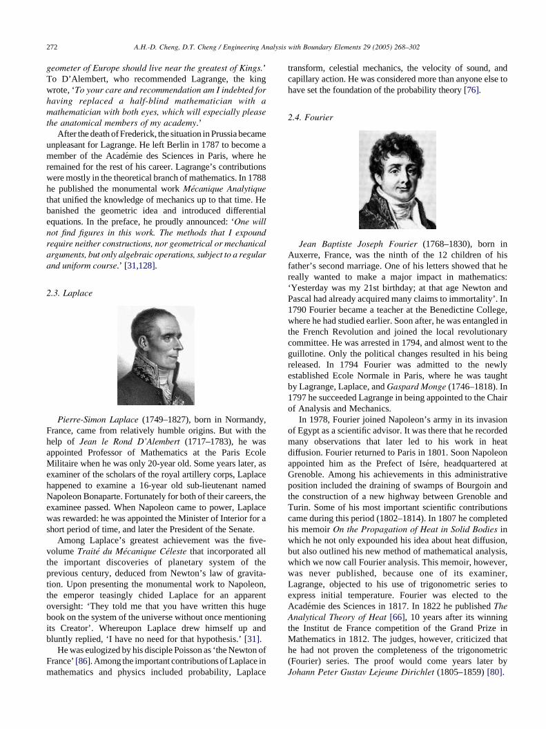
2.4. Fourier

Jean Baptiste Joseph Fourier (1768–1830), born in

Auxerre, France, was the ninth of the 12 children of his

father’s second marriage. One of his letters showed that he

really wanted to make a major impact in mathematics:

‘Yesterday was my 21st birthday; at that age Newton and

Pascal had already acquired many claims to immortality’. In

1790 Fourier became a teacher at the Benedictine College,

where he had studied earlier. Soon after, he was entangled in

the French Revolution and joined the local revolutionary

committee. He was arrested in 1794, and almost went to the

guillotine. Only the political changes resulted in his being

released. In 1794 Fourier was admitted to the newly

established Ecole Normale in Paris, where he was taught

by Lagrange, Laplace, and Gaspard Monge (1746–1818). In

1797 he succeeded Lagrange in being appointed to the Chair

of Analysis and Mechanics.

In 1978, Fourier joined Napoleon’s army in its invasion

of Egypt as a scientific advisor. It was there that he recorded

many observations that later led to his work in heat

diffusion. Fourier returned to Paris in 1801. Soon Napoleon

appointed him as the Prefect of Isere, headquartered at

Grenoble. Among his achievements in this administrative

position included the draining of swamps of Bourgoin and

the construction of a new highway between Grenoble and

Turin. Some of his most important scientific contributions

came during this period (1802–1814). In 1807 he completed

his memoir On the Propagation of Heat in Solid Bodies in

which he not only expounded his idea about heat diffusion,

but also outlined his new method of mathematical analysis,

which we now call Fourier analysis. This memoir, however,

was never published, because one of its examiner,

Lagrange, objected to his use of trigonometric series to

express initial temperature. Fourier was elected to the

Academie des Sciences in 1817. In 1822 he published The

Analytical Theory of Heat [66], 10 years after its winning

the Institut de France competition of the Grand Prize in

Mathematics in 1812. The judges, however, criticized that

he had not proven the completeness of the trigonometric

(Fourier) series. The proof would come years later by

Johann Peter Gustav Lejeune Dirichlet (1805–1859) [80].

A.H.-D. Cheng, D.T. Cheng / Engineering Analysis with Boundary Elements 29 (2005) 268–302 273

2.5. Poisson

Simeon-Denis Poisson (1781–1840) was born in Pithi-

viers, France. In 1796 Poisson was sent to Fontainebleau to

enroll in the Ecole Centrale. He soon showed great talents

for learning, especially mathematics. His teachers at the

Ecole Centrale were highly impressed and encouraged him

to sit in the entrance examinations for the Ecole Poly-

technique in Paris, the premiere institution at the time.

Although he had far less formal education than most of the

students taking the examinations, he achieved the top place.

His teachers Laplace and Lagrange quickly saw his

mathematical talents and they became friends for life. In

his final year of study he wrote a paper on the theory of

equations and Bezout’s theorem, and this was of such

quality that he was allowed to graduate in 1800 without

taking the final examination. He proceeded immediately to

the position equivalent to the present-day Assistant

Professor in the Ecole Polytechnique at the age of 19,

mainly on the strong recommendation of Laplace. It was

quite unusual for anyone to gain their first appointment in

Paris, as most of the top mathematicians had to serve in the

provinces before returning to Paris. Poisson was named

Associate Professor in 1802, and Professor in 1806 to fill the

position vacated by Fourier when he was sent by Napoleon

to Grenoble. In 1813 in his effort to answer the challenge

question for the election to the Academie des Sciences, he

developed the Poisson eqaution (12) to solve the electrical

field caused by distributed electrical charges in a body.

Poisson made great contributions in both mathematics

and physics. His name is attached to a wide variety of ideas,

for example, Poisson’s integral, Poisson equation, Poisson

brackets in differential equations, Poisson’s ratio in

elasticity, and Poisson’s constant in electricity [128].

2.6. Hamilton

William Rowan Hamilton (1805–1865) was a precocious

child. At the age of 5, he read Greek, Hebrew, and Latin; at

10, he was acquainted with half a dozen of oriental

languages. He entered Trinity College, Dublin at the age

of 18. His performance was so outstanding that he was

appointed Professor of Astronomy and the Royal Astron-

omer of Ireland when he was still an undergraduate at

Trinity. Hamilton was knighted at the age of 30 for the

scientific work he had already achieved.

Among Hamilton’s most important contributions is the

establishment of an analogy between the optical theory of

systems of rays and the dynamics of moving bodies. With

the further development by Carl Gustav Jacobi (1804–

1851), this theory is generally known as the Hamilton–

Jacobi Principle. By this construction, for example, it was

possible to determine the 10 planetary orbits around the sun,

a feat normally required the solution of 30 ordinary

differential equations, by merely two equations involving

Hamilton’s characteristic functions. However, this method

was more elegant than practical; hence for almost a century,

Hamilton’s great method was more praised than used [129].

This situation, however, changed when Irwin Schrodin-

ger (1887–1961) introduced the revolutionary wave-func-

tion model for quantum mechanics in 1926. Schrodinger

had expressed Hamilton’s significance quite unequivocally:

‘The modern development of physics is constantly enhan-

cing Hamilton’s name. His famous analogy between optics

and mechanics virtually anticipated wave mechanics, which

did not have much to add to his ideas and only had to take

them more seriously . If you wish to apply modern theory

to any particular problem, you must start with putting the

problem in Hamiltonian form’ [15].

3. Existence and uniqueness

The potential problems we solve are normally posed as

boundary value problems For example, given a closed

region U with the boundary G and the boundary condition

f Z f ðxÞ; x2G (13)

where f(x) is a continuous function, we are asked to find a

harmonic function (meaning a function satisfying the

Laplace equation) f(x) that fulfills the boundary condition

(13). This is known as the Dirichlet problem, named after

Dirichlet. The corresponding problem of finding a harmonic

function with the normal derivative boundary condition

vf

vnZ gðxÞ; x2G (14)

where n is the outward normal of G, is called the Neumann

problem, after Carl Gottfried Neumann (1832–1925).

The question of whether a solution of a Dirichlet or a

Neumann problem exists, and when it exists, whether it is

unique or not, is of great importance in mathematics and

physics alike. Obviously, if we cannot guarantee

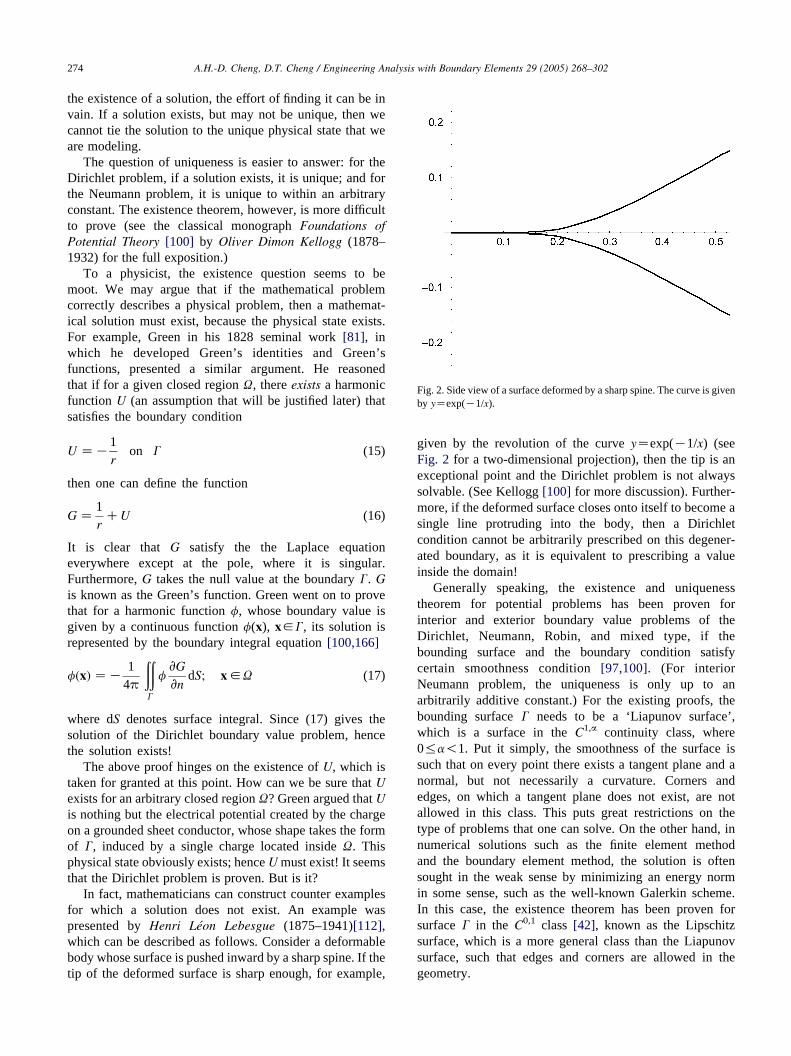
Fig. 2. Side view of a surface deformed by a sharp spine. The curve is given

by yZexp(K1/x).

A.H.-D. Cheng, D.T. Cheng / Engineering Analysis with Boundary Elements 29 (2005) 268–302274

the existence of a solution, the effort of finding it can be in

vain. If a solution exists, but may not be unique, then we

cannot tie the solution to the unique physical state that we

are modeling.

The question of uniqueness is easier to answer: for the

Dirichlet problem, if a solution exists, it is unique; and for

the Neumann problem, it is unique to within an arbitrary

constant. The existence theorem, however, is more difficult

to prove (see the classical monograph Foundations of

Potential Theory [100] by Oliver Dimon Kellogg (1878–

1932) for the full exposition.)

To a physicist, the existence question seems to be

moot. We may argue that if the mathematical problem

correctly describes a physical problem, then a mathemat-

ical solution must exist, because the physical state exists.

For example, Green in his 1828 seminal work [81], in

which he developed Green’s identities and Green’s

functions, presented a similar argument. He reasoned

that if for a given closed region U, there exists a harmonic

function U (an assumption that will be justified later) that

satisfies the boundary condition

U ZK1

ron G (15)

then one can define the function

G Z1

rCU (16)

It is clear that G satisfy the the Laplace equation

everywhere except at the pole, where it is singular.

Furthermore, G takes the null value at the boundary G. G

is known as the Green’s function. Green went on to prove

that for a harmonic function f, whose boundary value is

given by a continuous function f(x), x2G, its solution is

represented by the boundary integral equation [100,166]

fðxÞ ZK1

4p

ððG

fvG

vndS; x2U (17)

where dS denotes surface integral. Since (17) gives the

solution of the Dirichlet boundary value problem, hence

the solution exists!

The above proof hinges on the existence of U, which is

taken for granted at this point. How can we be sure that U

exists for an arbitrary closed region U? Green argued that U

is nothing but the electrical potential created by the charge

on a grounded sheet conductor, whose shape takes the form

of G, induced by a single charge located inside U. This

physical state obviously exists; hence U must exist! It seems

that the Dirichlet problem is proven. But is it?

In fact, mathematicians can construct counter examples

for which a solution does not exist. An example was

presented by Henri Leon Lebesgue (1875–1941)[112],

which can be described as follows. Consider a deformable

body whose surface is pushed inward by a sharp spine. If the

tip of the deformed surface is sharp enough, for example,

given by the revolution of the curve yZexp(K1/x) (see

Fig. 2 for a two-dimensional projection), then the tip is an

exceptional point and the Dirichlet problem is not always

solvable. (See Kellogg [100] for more discussion). Further-

more, if the deformed surface closes onto itself to become a

single line protruding into the body, then a Dirichlet

condition cannot be arbitrarily prescribed on this degener-

ated boundary, as it is equivalent to prescribing a value

inside the domain!

Generally speaking, the existence and uniqueness

theorem for potential problems has been proven for

interior and exterior boundary value problems of the

Dirichlet, Neumann, Robin, and mixed type, if the

bounding surface and the boundary condition satisfy

certain smoothness condition [97,100]. (For interior

Neumann problem, the uniqueness is only up to an

arbitrarily additive constant.) For the existing proofs, the

bounding surface G needs to be a ‘Liapunov surface’,

which is a surface in the C1,a continuity class, where

0%a!1. Put it simply, the smoothness of the surface is

such that on every point there exists a tangent plane and a

normal, but not necessarily a curvature. Corners and

edges, on which a tangent plane does not exist, are not

allowed in this class. This puts great restrictions on the

type of problems that one can solve. On the other hand, in

numerical solutions such as the finite element method

and the boundary element method, the solution is often

sought in the weak sense by minimizing an energy norm

in some sense, such as the well-known Galerkin scheme.

In this case, the existence theorem has been proven for

surface G in the C0,1 class [42], known as the Lipschitz

surface, which is a more general class than the Liapunov

surface, such that edges and corners are allowed in the

geometry.

A.H.-D. Cheng, D.T. Cheng / Engineering Analysis with Boundary Elements 29 (2005) 268–302 275

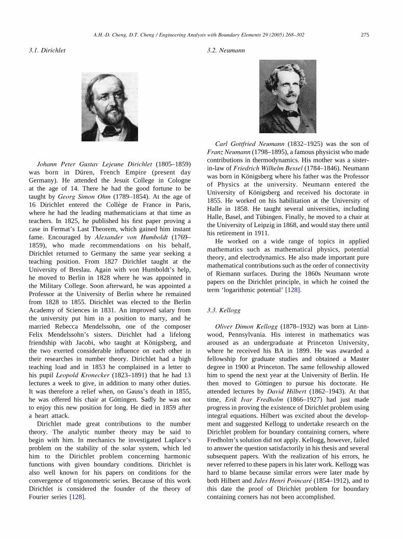
3.1. Dirichlet

Johann Peter Gustav Lejeune Dirichlet (1805–1859)

was born in Duren, French Empire (present day

Germany). He attended the Jesuit College in Cologne

at the age of 14. There he had the good fortune to be

taught by Georg Simon Ohm (1789–1854). At the age of

16 Dirichlet entered the College de France in Paris,

where he had the leading mathematicians at that time as

teachers. In 1825, he published his first paper proving a

case in Fermat’s Last Theorem, which gained him instant

fame. Encouraged by Alexander von Humboldt (1769–

1859), who made recommendations on his behalf,

Dirichlet returned to Germany the same year seeking a

teaching position. From 1827 Dirichlet taught at the

University of Breslau. Again with von Humboldt’s help,

he moved to Berlin in 1828 where he was appointed in

the Military College. Soon afterward, he was appointed a

Professor at the University of Berlin where he remained

from 1828 to 1855. Dirichlet was elected to the Berlin

Academy of Sciences in 1831. An improved salary from

the university put him in a position to marry, and he

married Rebecca Mendelssohn, one of the composer

Felix Mendelssohn’s sisters. Dirichlet had a lifelong

friendship with Jacobi, who taught at Konigsberg, and

the two exerted considerable influence on each other in

their researches in number theory. Dirichlet had a high

teaching load and in 1853 he complained in a letter to

his pupil Leopold Kronecker (1823–1891) that he had 13

lectures a week to give, in addition to many other duties.

It was therefore a relief when, on Gauss’s death in 1855,

he was offered his chair at Gottingen. Sadly he was not

to enjoy this new position for long. He died in 1859 after

a heart attack.

Dirichlet made great contributions to the number

theory. The analytic number theory may be said to

begin with him. In mechanics he investigated Laplace’s

problem on the stability of the solar system, which led

him to the Dirichlet problem concerning harmonic

functions with given boundary conditions. Dirichlet is

also well known for his papers on conditions for the

convergence of trigonometric series. Because of this work

Dirichlet is considered the founder of the theory of

Fourier series [128].

3.2. Neumann

Carl Gottfried Neumann (1832–1925) was the son of

Franz Neumann (1798–1895), a famous physicist who made

contributions in thermodynamics. His mother was a sister-

in-law of Friedrich Wilhelm Bessel (1784–1846). Neumann

was born in Konigsberg where his father was the Professor

of Physics at the university. Neumann entered the

University of Konigsberg and received his doctorate in

1855. He worked on his habilitation at the University of

Halle in 1858. He taught several universities, including

Halle, Basel, and Tubingen. Finally, he moved to a chair at

the University of Leipzig in 1868, and would stay there until

his retirement in 1911.

He worked on a wide range of topics in applied

mathematics such as mathematical physics, potential

theory, and electrodynamics. He also made important pure

mathematical contributions such as the order of connectivity

of Riemann surfaces. During the 1860s Neumann wrote

papers on the Dirichlet principle, in which he coined the

term ‘logarithmic potential’ [128].

3.3. Kellogg

Oliver Dimon Kellogg (1878–1932) was born at Linn-

wood, Pennsylvania. His interest in mathematics was

aroused as an undergraduate at Princeton University,

where he received his BA in 1899. He was awarded a

fellowship for graduate studies and obtained a Master

degree in 1900 at Princeton. The same fellowship allowed

him to spend the next year at the University of Berlin. He

then moved to Gottingen to pursue his doctorate. He

attended lectures by David Hilbert (1862–1943). At that

time, Erik Ivar Fredholm (1866–1927) had just made

progress in proving the existence of Dirichlet problem using

integral equations. Hilbert was excited about the develop-

ment and suggested Kellogg to undertake research on the

Dirichlet problem for boundary containing corners, where

Fredholm’s solution did not apply. Kellogg, however, failed

to answer the question satisfactorily in his thesis and several

subsequent papers. With the realization of his errors, he

never referred to these papers in his later work. Kellogg was

hard to blame because similar errors were later made by

both Hilbert and Jules Henri Poincare (1854–1912), and to

this date the proof of Dirichlet problem for boundary

containing corners has not been accomplished.

A.H.-D. Cheng, D.T. Cheng / Engineering Analysis with Boundary Elements 29 (2005) 268–302276

Kellogg received his PhD in 1903 and returned to the

United States to take up a post of instructor in mathematics

at Princeton. Two years later he joined the University of

Missouri as an Assistant Professor. He spent the next 14

fruitful years at Missouri until he was called by Harvard

University in 1919. Kellogg continued to work at Harvard

until his death from a heart attack suffered while climbing

[13,59]. His book ‘Foundations of Potential Theory’ [100],

first published in 1929, remains among the most author-

itative work to this date.

4. Reduction in dimension and Green’s formula

A key to the success of boundary element method is the

reduction of spatial dimension in its integral equation

representation, leading to a more efficient numerical

discretization. One of the most celebrated technique of

this type is the divergence theorem, which transforms a

volume integral into a surface integralðððU

V$A dV Z

ððG

A$n dS (18)

where A is a vector, n is the unit outward normal of G, and

dV stands for volume integral. Early development of this

type was found in the work of Lagrange [110] and Laplace.

Eq. (18), also called Gauss’s theorem, is commonly

attributed to Gauss [70]. However, Gauss in 1813 only

presented a few special cases in the form [99]ððG

nx dS Z 0 (19)

where nx is the x-component of outward normal, andððG

A$n dS Z 0 (20)

where the components of A are given by AxZAx(y,z), AyZAy(x,z), and AzZAz(x,y). The general theorem should be

credited to Mikhail Vasilevich Ostrogradski (1801–1862),

who in 1826 presented the following result to the Paris

Academie des Sciences [99]ðððU

a$Vf dV Z

ððG

fa$n dS (21)

where a is a constant vector.

Another useful formula is the Stokes’s theorem,

presented by George Gabriel Stokes (1819–1903), which

transforms a surface integral into a contour integral [162]ððS

ðV!AÞ$n dS Z

ðC

A$ds (22)

where S is an open, two sided curve surface, C is the closed

contour bounding S, and ds denotes line integral.

The most important work related to the boundary integral

equation solving potential problems came from George

Green, whose groundbreaking work remained obscure

during his lifetime, and he earned his fame only post-

humously. Green in 1828 [81] presented the three Green’s

identities. The first identity isðððU

ðfV2j CVf$VjÞ dV Z

ððG

fvj

vndS (23)

The above equation easily leads to the second identityðððU

ðfV2j KjV

2fÞ dV Z

ððG

fvj

vnKj

vf

vn

� �dS (24)

Using the fundamental solution of Laplace equation 1/r in

(24), the third identity is obtained

f Z1

4p

ððG

1

r

vf

vnKf

vð1=rÞ

vn

� �dS (25)

which is exactly the formulation of the present-day

boundary element method for potential problems.

4.1. Gauss

Carl Friedrich Gauss (1777–1855) was born an infant

prodigy into a poor and unlettered family. According to a

well-authenticated story, he corrected an error in his father’s

payroll calculations as a child of three. He was supported by

the Duke Ferdinand of Braunschweig to receive his

education. Even as a student, he made major discoveries,

including the method of least squares and the discovery of

how to construct the regular 17-gon. However, his early

career was not very successful and had to continue to rely on

the financial support of his benefactor. At the age of 22, he

published as his doctoral thesis the most celebrated work,

the Fundamental Theorem of Algebra. In 1807 Gauss was

finally able to secure a position as the Director of the newly

founded observatory at the Gottingen University, a job he

held for the rest of his life.

Gauss devoted more of his time in theoretical astronomy

than in mathematics. This is considered a great loss for

mathematics—just imagine how much more mathematics he

could have accomplished. He devised a procedure for

calculating the orbits planetoids that included the use of

least square that he developed. Using his superior method,

A.H.-D. Cheng, D.T. Cheng / Engineering Analysis with Boundary Elements 29 (2005) 268–302 277

Gauss redid in an hour’s time the calculation on which Euler

had spent 3 days, and which sometimes was said to have led to

Euler’s loss of sight. Gauss remarked unkindly, ‘I should also

have gone blind if I had calculated in that fashion for 3 days’.

Gauss not only adorned every branches of pure

mathematics and was called the Prince of Mathematicians,

he also pursued work in several related scientific fields,

notably physics, mechanics, and astronomy. Together with

Wilhelm Eduard Weber (1804–1891), he studied electro-

magnetism. They were the first to have successfully

transmitted telegraph [30,31].

4.2. Green

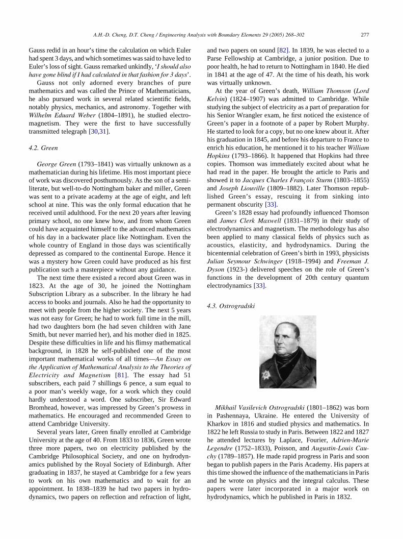
George Green (1793–1841) was virtually unknown as a

mathematician during his lifetime. His most important piece

of work was discovered posthumously. As the son of a semi-

literate, but well-to-do Nottingham baker and miller, Green

was sent to a private academy at the age of eight, and left

school at nine. This was the only formal education that he

received until adulthood. For the next 20 years after leaving

primary school, no one knew how, and from whom Green

could have acquainted himself to the advanced mathematics

of his day in a backwater place like Nottingham. Even the

whole country of England in those days was scientifically

depressed as compared to the continental Europe. Hence it

was a mystery how Green could have produced as his first

publication such a masterpiece without any guidance.

The next time there existed a record about Green was in

1823. At the age of 30, he joined the Nottingham

Subscription Library as a subscriber. In the library he had

access to books and journals. Also he had the opportunity to

meet with people from the higher society. The next 5 years

was not easy for Green; he had to work full time in the mill,

had two daughters born (he had seven children with Jane

Smith, but never married her), and his mother died in 1825.

Despite these difficulties in life and his flimsy mathematical

background, in 1828 he self-published one of the most

important mathematical works of all times—An Essay on

the Application of Mathematical Analysis to the Theories of

Electricity and Magnetism [81]. The essay had 51

subscribers, each paid 7 shillings 6 pence, a sum equal to

a poor man’s weekly wage, for a work which they could

hardly understood a word. One subscriber, Sir Edward

Bromhead, however, was impressed by Green’s prowess in

mathematics. He encouraged and recommended Green to

attend Cambridge University.

Several years later, Green finally enrolled at Cambridge

University at the age of 40. From 1833 to 1836, Green wrote

three more papers, two on electricity published by the

Cambridge Philosophical Society, and one on hydrodyn-

amics published by the Royal Society of Edinburgh. After

graduating in 1837, he stayed at Cambridge for a few years

to work on his own mathematics and to wait for an

appointment. In 1838–1839 he had two papers in hydro-

dynamics, two papers on reflection and refraction of light,

and two papers on sound [82]. In 1839, he was elected to a

Parse Fellowship at Cambridge, a junior position. Due to

poor health, he had to return to Nottingham in 1840. He died

in 1841 at the age of 47. At the time of his death, his work

was virtually unknown.

At the year of Green’s death, William Thomson (Lord

Kelvin) (1824–1907) was admitted to Cambridge. While

studying the subject of electricity as a part of preparation for

his Senior Wrangler exam, he first noticed the existence of

Green’s paper in a footnote of a paper by Robert Murphy.

He started to look for a copy, but no one knew about it. After

his graduation in 1845, and before his departure to France to

enrich his education, he mentioned it to his teacher William

Hopkins (1793–1866). It happened that Hopkins had three

copies. Thomson was immediately excited about what he

had read in the paper. He brought the article to Paris and

showed it to Jacques Charles Francois Sturm (1803–1855)

and Joseph Liouville (1809–1882). Later Thomson repub-

lished Green’s essay, rescuing it from sinking into

permanent obscurity [33].

Green’s 1828 essay had profoundly influenced Thomson

and James Clerk Maxwell (1831–1879) in their study of

electrodynamics and magnetism. The methodology has also

been applied to many classical fields of physics such as

acoustics, elasticity, and hydrodynamics. During the

bicentennial celebration of Green’s birth in 1993, physicists

Julian Seymour Schwinger (1918–1994) and Freeman J.

Dyson (1923-) delivered speeches on the role of Green’s

functions in the development of 20th century quantum

electrodynamics [33].

4.3. Ostrogradski

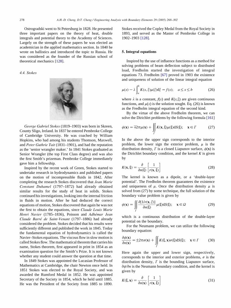
Mikhail Vasilevich Ostrogradski (1801–1862) was born

in Pashennaya, Ukraine. He entered the University of

Kharkov in 1816 and studied physics and mathematics. In

1822 he left Russia to study in Paris. Between 1822 and 1827

he attended lectures by Laplace, Fourier, Adrien-Marie

Legendre (1752–1833), Poisson, and Augustin-Louis Cau-

chy (1789–1857). He made rapid progress in Paris and soon

began to publish papers in the Paris Academy. His papers at

this time showed the influence of the mathematicians in Paris

and he wrote on physics and the integral calculus. These

papers were later incorporated in a major work on

hydrodynamics, which he published in Paris in 1832.

A.H.-D. Cheng, D.T. Cheng / Engineering Analysis with Boundary Elements 29 (2005) 268–302278

Ostrogradski went to St Petersburg in 1828. He presented

three important papers on the theory of heat, double

integrals and potential theory to the Academy of Sciences.

Largely on the strength of these papers he was elected an

academician in the applied mathematics section. In 1840 he

wrote on ballistics and introduced the topic to Russia. He

was considered as the founder of the Russian school of

theoretical mechanics [128].

4.4. Stokes

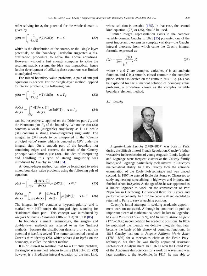
George Gabriel Stokes (1819–1903) was born in Skreen,

County Sligo, Ireland. In 1837 he entered Pembroke College

of Cambridge University. He was coached by William

Hopkins, who had among his students Thomson, Maxwell,

and Peter Guthrie Tait (1831–1901), and had the reputation

as the ‘senior wrangler maker.’ In 1841 Stokes graduated as

Senior Wrangler (the top First Class degree) and was also

the first Smith’s prizeman. Pembroke College immediately

gave him a fellowship.

Inspired by the recent work of Green, Stokes started to

undertake research in hydrodynamics and published papers

on the motion of incompressible fluids in 1842. After

completing the research Stokes discovered that Jean Marie

Constant Duhamel (1797–1872) had already obtained

similar results for the study of heat in solids. Stokes

continued his investigations, looking into the internal friction

in fluids in motion. After he had deduced the correct

equations of motion, Stokes discovered that again he was not

the first to obtain the equations, since Claude Louis Marie

Henri Navier (1785–1836), Poisson and Adhemar Jean

Claude Barre de Saint-Venant (1797–1886) had already

considered the problem. Stokes decided that his results were

sufficiently different and published the work in 1845. Today

the fundamental equation of hydrodynamics is called the

Navier–Stokes equations. The viscous flow in slow motion is

called Stokes flow. The mathematical theorem that carries his

name, Stokes theorem, first appeared in print in 1854 as an

examination question for the Smith’s Prize. It is not known

whether any student could answer the question at that time.

In 1849 Stokes was appointed the Lucasian Professor of

Mathematics at Cambridge, the chair Newton once held. In

1851 Stokes was elected to the Royal Society, and was

awarded the Rumford Medal in 1852. He was appointed

Secretary of the Society in 1854, which he held until 1885.

He was the President of the Society from 1885 to 1890.

Stokes received the Copley Medal from the Royal Society in

1893, and served as the Master of Pembroke College in

1902–1903 [128].

5. Integral equations

Inspired by the use of influence functions as a method for

solving problems of beam deflection subject to distributed

load, Fredholm started the investigation of integral

equations 73. Fredholm [67] proved in 1903 the existence

and uniqueness of solution of the linear integral equation

mðxÞKl

ðb

aKðx; xÞmðxÞdx Z f ðxÞ; a%x%b (26)

where l is a constant, f(x) and K(x,x) are given continuous

functions, and m(x) is the solution sought. Eq. (26) is known

as the Fredholm integral equation of the second kind.

By the virtue of the above Fredholm theorem, we can

solve the Dirichlet problems by the following formula [161]

fðxÞ ZH2pmðxÞC

ððG

Kðx; xÞmðxÞdSðxÞ; x2G (27)

In the above the upper sign corresponds to the interior

problem, the lower sign the exterior problem, m is the

distribution density, G is a closed Liapunov surface, f(x) is

the Dirichlet boundary condition, and the kernel K is given

by

Kðx; xÞ Zv

vnðxÞ

1

rðx; xÞ

� �(28)

The kernel is known as a dipole, or a ‘double-layer

potential’. The Fredholm theorem guarantees the existence

and uniqueness of m. Once the distribution density m is

solved from (27) by some technique, the full solution of the

boundary value problem is given by

fðxÞ Z

ððG

v½1=rðx; xÞ�

vnðxÞmðxÞdSðxÞ; x2U (29)

which is a continuous distribution of the double-layer

potential on the boundary.

For the Neumann problem, we can utilize the following

boundary equation:

vfðxÞ

vnðxÞZG2psðxÞC

ððG

Kðx; xÞsðxÞdSðxÞ; x2G (30)

Here again the upper and lower sign, respectively,

corresponds to the interior and exterior problems, s is the

distribution density, G is the bounding Liapunov surface,

vf/vn is the Neumann boundary condition, and the kernel is

given by

Kðx; xÞ Zv

vnðxÞ

1

rðx; xÞ

� �(31)

A.H.-D. Cheng, D.T. Cheng / Engineering Analysis with Boundary Elements 29 (2005) 268–302 279

After solving for s, the potential for the whole domain is

given by

fðxÞ Z

ððG

1

rðx; xÞsðxÞdSðxÞ; x2U (32)

which is the distribution of the source, or the ‘single-layer

potential’, on the boundary. Fredholm suggested a dis-

cretization procedure to solve the above equations.

However, without a fast enough computer to solve the

resultant matrix system, the idea was impractical; hence

further development of utilizing these equations was limited

to analytical work.

For mixed boundary value problems, a pair of integral

equations is needed. For the ‘single-layer method’ applied

to interior problems, the following pair

fðxÞ Z

ððG

1

rðx; xÞsðxÞdSðxÞ; x2Gf (33)

vfðxÞ

vnðxÞZ

ððCPV

v½1=rðx; xÞ�

vnðxÞsðxÞdSðxÞ; x2Gq (34)

can be, respectively, applied on the Dirichlet part Gf and

the Neumann part Gq of the boundary. We notice that (33)

contains a weak (integrable) singularity as x/x; while

(34) contains a strong (non-integrable) singularity. The

integral in (34) needs to be interpreted in the ‘Cauchy

principal value’ sense, which is denoted as CPV under the

integral sign. On a smooth part of the boundary not

containing edges and corners, the result of the Cauchy

principle value limit is just (30). This idea of interpreting

and handling this type of strong singularity was

introduced by Cauchy in 1814 [34].

A ‘double-layer method’ can also be formulated to solve

mixed boundary value problems using the following pair of

equations

fðxÞ Z

ððCPV

v½1=rðx; xÞ�

vnðxÞmðxÞdSðxÞ; x2G (35)

vfðxÞ

vnðxÞZ

ððHFP

v

vnðxÞ

v1=rðx; xÞ

vnðxÞ

� �mðxÞdSðxÞ; x2G (36)

The integral in (36) contains a ‘hypersingularity’ and is

marked with HFP under the integral sign, standing for

‘Hadamard finite part.’ This concept was introduced by

Jacques Salomon Hadamard (1865–1963) in 1908 [85].

In boundary element terminology, the single- and

double-layer methods are referred to as the ‘indirect

methods,’ because the distribution density m or s, not the

potential f itself, is solved. The numerical method based on

Green’s third identity (25), which solves f or vf/vn on the

boundary, is called the ‘direct method’.

It is of interest to mention that for a Dirichlet problem,

the single-layer method reduces to using (33) only. Eq. (33)

however is a Fredholm integral equation of the first kind,

whose solution is unstable [175]. In that case, the second

kind equation, (27) or (35), should be used.

Similar integral representation exists in the complex

variable domain. Cauchy in 1825 [35] presented one of the

most important theorems in complex variable—the Cauchy

integral theorem, from which came the Cauchy integral

formula, expressed as

f ðzÞ Z1

2pi

ðC

f ðzÞ

z Kzdz (37)

where z and z are complex variables, f is an analytic

function, and C is a smooth, closed contour in the complex

plane. When z is located on the contour, z2C, Eq. (37) can

be exploited for the numerical solution of boundary value

problems, a procedure known as the complex variable

boundary element method.

5.1. Cauchy

Augustin-Louis Cauchy (1789–1857) was born in Paris

during the difficult time of French Revolution. Cauchy’s father

was active in the education of young Augustin-Louis. Laplace

and Lagrange were frequent visitors at the Cauchy family

home, and Lagrange particularly took interest in Cauchy’s

mathematical ability. In 1805 Cauchy took the entrance

examination of the Ecole Polytechnique and was placed

second. In 1807 he entered Ecole des Ponts et Chaussees to

study engineering, specializing in highways and bridges, and

finished school in 2 years. At the age of 20, he was appointed as

a Junior Engineer to work on the construction of Port

Napoleon in Cherbourg. He worked there for 3 years and

performed excellently. In 1812, he became ill and decided to

returned to Paris to seek a teaching position.

Cauchy’s initial attempts in seeking academic appoint-

ment were unsuccessful. Although he continued to publish

important pieces of mathematical work, he lost to Legendre,

to Louis Poinsot (1777–1859), and to Andre Marie Ampere

(1775–1836) in competition for academic positions. In 1814

he published the memoir on definite integrals that later

became the basis of his theory of complex functions. In

1815 Cauchy lost out to Jacques Philippe Marie Binet

(1786–1856) for a mechanics chair at the Ecole Poly-

technique, but then he was finally appointed Assistant

Professor of Analysis there. In 1816 he won the Grand Prix

of the Academie des Sciences for a work on waves, and was

later admitted to the Academie. In 1817, he was able to

A.H.-D. Cheng, D.T. Cheng / Engineering Analysis with Boundary Elements 29 (2005) 268–302280

substitute for Jean-Baptiste Biot (1774–1862), Chair of

Mathematical Physics at the College de France, and later for

Poisson. It was not until 1821 that he was able to obtain a

full position replacing Ampere.

Cauchy was staunchly Catholic and was politically a

royalist. By 1830 the political events in Paris forced him to

leave Paris for Switzerland. He soon lost all his positions in

Paris. In 1831 Cauchy went to Turin and later accepted an

offer to become a Chair of Theoretical Physics. In 1833

Cauchy went from Turin to Prague, and returned to Paris in

1838. He regained his position at the Academie but not his

teaching positions because he had refused to take an oath of

allegiance to the new regime. Due to his political and

religious views, he continued to have difficulty in getting

appointment.

Cauchy was probably next to Euler the most published

author in mathematics, having produced five textbooks and

over 800 articles. Cauchy and his contemporary Gauss were

credited for introducing rigor into modern mathematics. It

was said that when Cauchy read to the Academie des

Sciences in Paris his first paper on the convergence of series,

Laplace hurried home to verify that he had not made mistake

of using any divergence series in his Mecanique Celeste. The

formulation of elementary calculus in modern textbooks is

essentially what Cauchy expounded in his three great

treatises: Cours d’Analyse de l’Ecole Royale Polytechnique

(1821), Resume des Lecons sur le Calcul Infinitesimal

(1823), and Lecons sur le Calcul Differentiel (1829). Cauchy

was also credited for setting the mathematical foundation for

complex variable and elasticity. The basic equation of

elasticity is called the Navier–Cauchy equation [8,79].

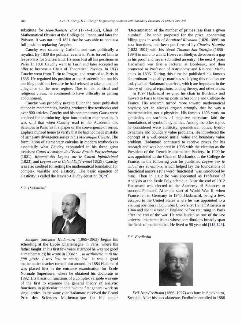
5.2. Hadamard

Jacques Salomon Hadamard (1865–1963) began his

schooling at the Lycee Charlemagne in Paris, where his

father taught. In his first few years at school he was not good

at mathematics; he wrote in 1936: ‘. in arithmetic, until the

fifth grade, I was last or nearly last’. It was a good

mathematics teacher turned him around. In 1884 Hadamard

was placed first in the entrance examination for Ecole

Normale Superieure, where he obtained his doctorate in

1892. His thesis on functions of a complex variable was one

of the first to examine the general theory of analytic

functions, in particular it contained the first general work on

singularities. In the same year Hadamard received the Grand

Prix des Sciences Mathematique for his paper

‘Determination of the number of primes less than a given

number’. The topic proposed for the prize, concerning

filling gaps in work of Bernhard Riemann (1826–1866) on

zeta functions, had been put forward by Charles Hermite

(1822–1901) with his friend Thomas Jan Stieltjes (1856–

1894) in mind to win it. However, Stieltjes discovered a gap

in his proof and never submitted an entry. The next 4 years

Hadamard was first a lecturer at Bordeaux, and then

promoted to Professor of Astronomy and Rational Mech-

anics in 1896. During this time he published his famous

determinant inequality; matrices satisfying this relation are

today called Hadamard matrices, which are important in the

theory of integral equations, coding theory, and other areas.

In 1897 Hadamard resigned his chair in Bordeaux and

moved to Paris to take up posts in Sorbonne and College de

France. His research turned more toward mathematical

physics; yet he always argued strongly that he was a

mathematician, not a physicist. His famous 1898 work on

geodesics on surfaces of negative curvature laid the

foundations of symbolic dynamics. Among the other topics

he considered were elasticity, geometrical optics, hydro-

dynamics and boundary value problems. He introduced the

concept of a well-posed initial value and boundary value

problem. Hadamard continued to receive prizes for his

research and was honored in 1906 with the election as the

President of the French Mathematical Society. In 1909 he

was appointed to the Chair of Mechanics at the College de

France. In the following year he published Lecons sur le

calcul des variations, which helped lay the foundations of

functional analysis (the word ‘functional’ was introduced by

him). Then in 1912 he was appointed as Professor of

Analysis at the Ecole Polytechnique. Near the end of 1912

Hadamard was elected to the Academy of Sciences to

succeed Poincare. After the start of World War II, when

France fell to Germany in 1940, Hadamard, being a Jew,

escaped to the United States where he was appointed to a

visiting position at Columbia University. He left America in

1944 and spent a year in England before returning to Paris

after the end of the war. He was lauded as one of the last

universal mathematicians whose contributions broadly span

the fields of mathematics. He lived to 98 year old [118,128].

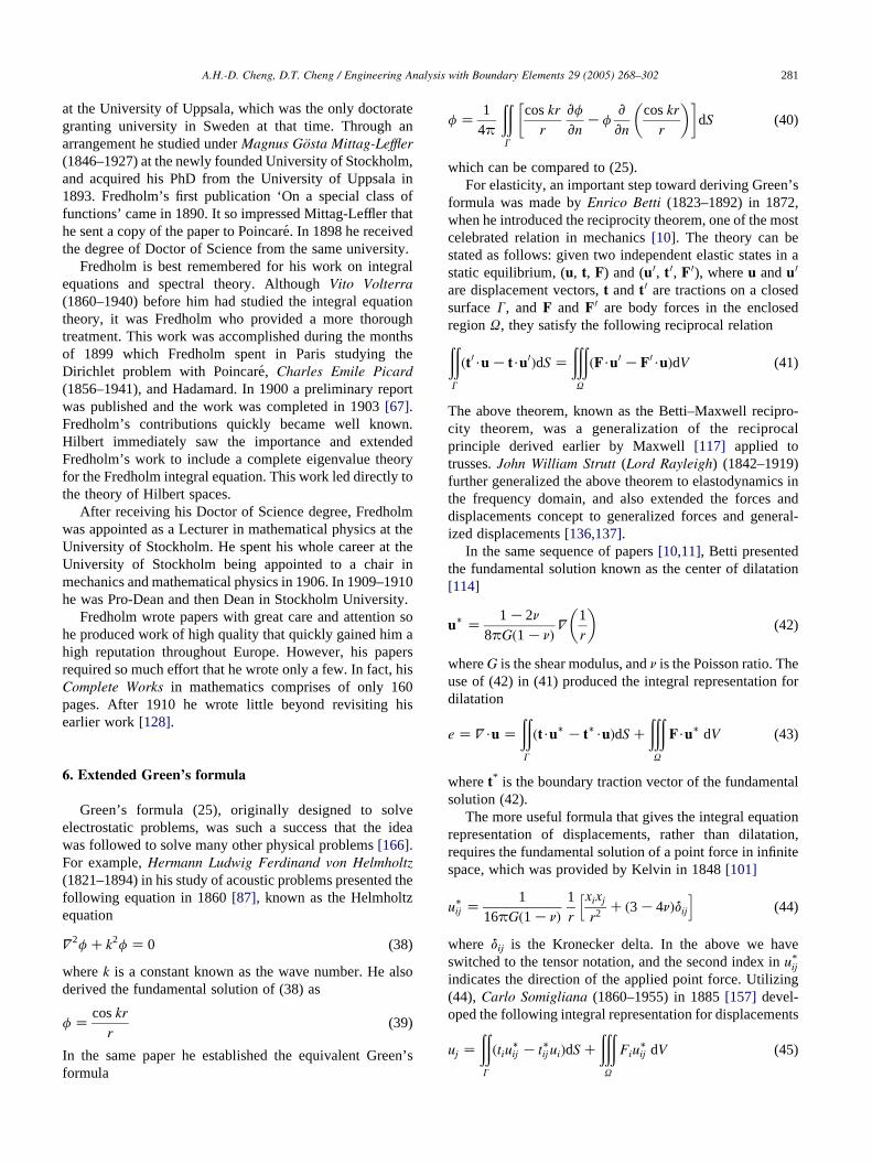
5.3. Fredholm

Erik Ivar Fredholm (1866–1927) was born in Stockholm,

Sweden. After his baccalaureate, Fredholm enrolled in 1886

A.H.-D. Cheng, D.T. Cheng / Engineering Analysis with Boundary Elements 29 (2005) 268–302 281

at the University of Uppsala, which was the only doctorate

granting university in Sweden at that time. Through an

arrangement he studied under Magnus Gosta Mittag-Leffler

(1846–1927) at the newly founded University of Stockholm,

and acquired his PhD from the University of Uppsala in

1893. Fredholm’s first publication ‘On a special class of

functions’ came in 1890. It so impressed Mittag-Leffler that

he sent a copy of the paper to Poincare. In 1898 he received

the degree of Doctor of Science from the same university.

Fredholm is best remembered for his work on integral

equations and spectral theory. Although Vito Volterra

(1860–1940) before him had studied the integral equation

theory, it was Fredholm who provided a more thorough

treatment. This work was accomplished during the months

of 1899 which Fredholm spent in Paris studying the

Dirichlet problem with Poincare, Charles Emile Picard

(1856–1941), and Hadamard. In 1900 a preliminary report

was published and the work was completed in 1903 [67].

Fredholm’s contributions quickly became well known.

Hilbert immediately saw the importance and extended

Fredholm’s work to include a complete eigenvalue theory

for the Fredholm integral equation. This work led directly to

the theory of Hilbert spaces.

After receiving his Doctor of Science degree, Fredholm

was appointed as a Lecturer in mathematical physics at the

University of Stockholm. He spent his whole career at the

University of Stockholm being appointed to a chair in

mechanics and mathematical physics in 1906. In 1909–1910

he was Pro-Dean and then Dean in Stockholm University.

Fredholm wrote papers with great care and attention so

he produced work of high quality that quickly gained him a

high reputation throughout Europe. However, his papers

required so much effort that he wrote only a few. In fact, his

Complete Works in mathematics comprises of only 160

pages. After 1910 he wrote little beyond revisiting his

earlier work [128].

6. Extended Green’s formula

Green’s formula (25), originally designed to solve

electrostatic problems, was such a success that the idea

was followed to solve many other physical problems [166].

For example, Hermann Ludwig Ferdinand von Helmholtz

(1821–1894) in his study of acoustic problems presented the

following equation in 1860 [87], known as the Helmholtz

equation

V2f Ck2f Z 0 (38)

where k is a constant known as the wave number. He also

derived the fundamental solution of (38) as

f Zcos kr

r(39)

In the same paper he established the equivalent Green’s

formula

f Z1

4p

ððG

cos kr

r

vf

vnKf

v

vn

cos kr

r

� �� �dS (40)

which can be compared to (25).

For elasticity, an important step toward deriving Green’s

formula was made by Enrico Betti (1823–1892) in 1872,

when he introduced the reciprocity theorem, one of the most

celebrated relation in mechanics [10]. The theory can be

stated as follows: given two independent elastic states in a

static equilibrium, (u, t, F) and (u 0, t 0, F 0), where u and u 0

are displacement vectors, t and t 0 are tractions on a closed

surface G, and F and F 0 are body forces in the enclosed

region U, they satisfy the following reciprocal relationððG

ðt0$u K t$u0ÞdS Z

ðððU

ðF$u0 KF0$uÞdV (41)

The above theorem, known as the Betti–Maxwell recipro-

city theorem, was a generalization of the reciprocal

principle derived earlier by Maxwell [117] applied to

trusses. John William Strutt (Lord Rayleigh) (1842–1919)

further generalized the above theorem to elastodynamics in

the frequency domain, and also extended the forces and

displacements concept to generalized forces and general-

ized displacements [136,137].

In the same sequence of papers [10,11], Betti presented

the fundamental solution known as the center of dilatation

[114]

u� Z1 K2n

8pGð1 KnÞV

1

r

� �(42)

where G is the shear modulus, and n is the Poisson ratio. The

use of (42) in (41) produced the integral representation for

dilatation

e Z V$u Z

ððG

ðt$u� K t�$uÞdS C

ðððU

F$u� dV (43)

where t* is the boundary traction vector of the fundamental

solution (42).

The more useful formula that gives the integral equation

representation of displacements, rather than dilatation,

requires the fundamental solution of a point force in infinite

space, which was provided by Kelvin in 1848 [101]

u�ij Z

1

16pGð1 KnÞ

1

r

xixj

r2C ð3 K4nÞdij

h i(44)

where dij is the Kronecker delta. In the above we have

switched to the tensor notation, and the second index in u*ij

indicates the direction of the applied point force. Utilizing

(44), Carlo Somigliana (1860–1955) in 1885 [157] devel-

oped the following integral representation for displacements

uj Z

ððG

ðtiu�ij K t�ij uiÞdS C

ðððU

Fiu�ij dV (45)

A.H.-D. Cheng, D.T. Cheng / Engineering Analysis with Boundary Elements 29 (2005) 268–302282

Eq. (45), called the Somigliana identity, is the elasticity

counterpart of Green’s formula (25).

Volterra [183] in 1907 presented the dislocation solution

of elasticity, as well as other singular solutions such as

the force double and the disclination, generally known as the

nuclei of strain [114]. Further dislocation solutions were

given by Somigliana in 1914 [158] and 1915 [159]. For a

point dislocation in unbounded three-dimensional space, the

resultant displacement field is

u�ijk Z

1

4pð1 KnÞ

!1

r2ð1 K2nÞðdkjxi Kdijxk KdikxjÞK

2

r2xixjxk

� �(46)

This singular solution can be distributed over the boundary

G to give the Volterra integral equation of the first kind

[182]

uk Z

ððG

u�kjinjmi dS C

ðððU

u�kiFi dV (47)

where mi is the component of the distribution density vector

m, also known as the displacement discontinuity. Eq. (47) is

equivalent to (35) of the potential problem, and can be called

the double-layer method. The counterpart of the single-layer

method (33) is given by the Somigliana integral equation

uj Z

ððG

u�jisi dS C

ðððU

u�jiFi dV (48)

where si is the component of the distribution density vector

s, known as the stress discontinuity.

Similar to Cauchy integral (37) for potential problems,

the complex variable potentials and integral equation

representation for elasticity exist, which was formulated

by Gury Vasilievich Kolosov (1867–1936) in 1909 [102].

These were further developed by Nikolai Ivanovich

Muskhelishvili (1891–1976) [125,126].

We can derive the above extended Green’s formulae in a

unified fashion. Consider the generalized Green’s theorem

[123]ðU

ðvLfugKuL�fvgÞdx Z

ðG

ðvBfugKuB�fvgÞdx (49)

In the above u and v are two independent vector functions, L

is a linear partial differential operator, L� is its adjoint

operator, B is the generalized boundary normal derivative,

and B� is its adjoint operator. The right hand side of (49) is

the consequence of integration by parts of the left hand side

operators. Eq. (49) may be compared with the Green’s

second identify (24). If we assume that u is the solution of

the homogeneous equations

LðuÞ Z 0 in U (50)

subject to certain boundary conditions, and v is replaced by

the fundamental solution of the adjoint operator satisfying

L�fGg Z d (51)

Eq. (49) becomes the boundary integral equation

u Z

ðG

ðuB�fGgKGBfugÞdx (52)

As an example, we consider the general second order linear

partial differential equation is two-dimension

Lfug Z Av2u

vx2C2B

v2u

vxvyCC

v2u

vy2CD

vu

vxCE

vu

vyCFu

(53)

where the coefficients A,B,., and F are functions of x and y.

The generalized Green’s second identity in the form of (49)

exists with the definition of the operators [83]

L�fvg Z

v2Av

vx2C2

v2Bv

vxvyC

v2Cv

vy2K

vDv

vxK

vEv

vyCFv

(54)

Bfug Z Avu

vxC2B

vu

vy

� �nx C C

vu

vyCEu

� �ny (55)

B�fvg Z

vAv

vxKDv

� �nx C 2

vBv

vxC

vCv

vy

� �ny (56)

If we require u and v to satisfy (50) and (51), respectively,

we then obtain the boundary integral equation formulation

(52).

6.1. Helmholtz

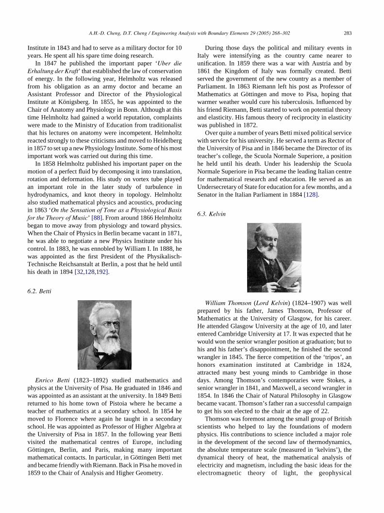
Hermann Ludwig Ferdinand von Helmholtz (1821–1894)

was born in Potsdam, Germany. He attended Potsdam

Gymnasium where his father was a teacher. His interests at

school were mainly in physics. However, due to the financial

situation of his family, he accepted a government grant to

study medicine at the Royal Friedrich-Wilhelm Institute of

Medicine and Surgery in Berlin. His research career began in

1841 when he worked on the connection between nerve fibers

and nerve cells for his dissertation. He rejected the dominant

physiology theory at that time, which was based on vital

forces, and strongly argued on the ground of physics and

chemistry principles. He graduated from the Medical

A.H.-D. Cheng, D.T. Cheng / Engineering Analysis with Boundary Elements 29 (2005) 268–302 283

Institute in 1843 and had to serve as a military doctor for 10

years. He spent all his spare time doing research.

In 1847 he published the important paper ‘Uber die

Erhaltung der Kraft’ that established the law of conservation

of energy. In the following year, Helmholtz was released

from his obligation as an army doctor and became an

Assistant Professor and Director of the Physiological

Institute at Konigsberg. In 1855, he was appointed to the

Chair of Anatomy and Physiology in Bonn. Although at this

time Helmholtz had gained a world reputation, complaints

were made to the Ministry of Education from traditionalist

that his lectures on anatomy were incompetent. Helmholtz

reacted strongly to these criticisms and moved to Heidelberg

in 1857 to set up a new Physiology Institute. Some of his most

important work was carried out during this time.

In 1858 Helmholtz published his important paper on the

motion of a perfect fluid by decomposing it into translation,

rotation and deformation. His study on vortex tube played

an important role in the later study of turbulence in

hydrodynamics, and knot theory in topology. Helmholtz

also studied mathematical physics and acoustics, producing

in 1863 ‘On the Sensation of Tone as a Physiological Basis

for the Theory of Music’ [88]. From around 1866 Helmholtz

began to move away from physiology and toward physics.

When the Chair of Physics in Berlin became vacant in 1871,

he was able to negotiate a new Physics Institute under his

control. In 1883, he was ennobled by William I. In 1888, he

was appointed as the first President of the Physikalisch-

Technische Reichsanstalt at Berlin, a post that he held until

his death in 1894 [32,128,192].

6.2. Betti

Enrico Betti (1823–1892) studied mathematics and

physics at the University of Pisa. He graduated in 1846 and

was appointed as an assistant at the university. In 1849 Betti

returned to his home town of Pistoia where he became a

teacher of mathematics at a secondary school. In 1854 he

moved to Florence where again he taught in a secondary

school. He was appointed as Professor of Higher Algebra at

the University of Pisa in 1857. In the following year Betti

visited the mathematical centres of Europe, including

Gottingen, Berlin, and Paris, making many important

mathematical contacts. In particular, in Gottingen Betti met

and became friendly with Riemann. Back in Pisa he moved in

1859 to the Chair of Analysis and Higher Geometry.

During those days the political and military events in

Italy were intensifying as the country came nearer to

unification. In 1859 there was a war with Austria and by

1861 the Kingdom of Italy was formally created. Betti

served the government of the new country as a member of

Parliament. In 1863 Riemann left his post as Professor of

Mathematics at Gottingen and move to Pisa, hoping that

warmer weather would cure his tuberculosis. Influenced by

his friend Riemann, Betti started to work on potential theory

and elasticity. His famous theory of reciprocity in elasticity

was published in 1872.

Over quite a number of years Betti mixed political service

with service for his university. He served a term as Rector of

the University of Pisa and in 1846 became the Director of its

teacher’s college, the Scuola Normale Superiore, a position

he held until his death. Under his leadership the Scuola

Normale Superiore in Pisa became the leading Italian centre

for mathematical research and education. He served as an

Undersecretary of State for education for a few months, and a

Senator in the Italian Parliament in 1884 [128].

6.3. Kelvin

William Thomson (Lord Kelvin) (1824–1907) was well

prepared by his father, James Thomson, Professor of

Mathematics at the University of Glasgow, for his career.

He attended Glasgow University at the age of 10, and later

entered Cambridge University at 17. It was expected that he

would won the senior wrangler position at graduation; but to

his and his father’s disappointment, he finished the second

wrangler in 1845. The fierce competition of the ‘tripos’, an

honors examination instituted at Cambridge in 1824,

attracted many best young minds to Cambridge in those

days. Among Thomson’s contemporaries were Stokes, a

senior wrangler in 1841, and Maxwell, a second wrangler in

1854. In 1846 the Chair of Natural Philosophy in Glasgow

became vacant. Thomson’s father ran a successful campaign

to get his son elected to the chair at the age of 22.

Thomson was foremost among the small group of British

scientists who helped to lay the foundations of modern

physics. His contributions to science included a major role

in the development of the second law of thermodynamics,

the absolute temperature scale (measured in ‘kelvins’), the

dynamical theory of heat, the mathematical analysis of

electricity and magnetism, including the basic ideas for the

electromagnetic theory of light, the geophysical

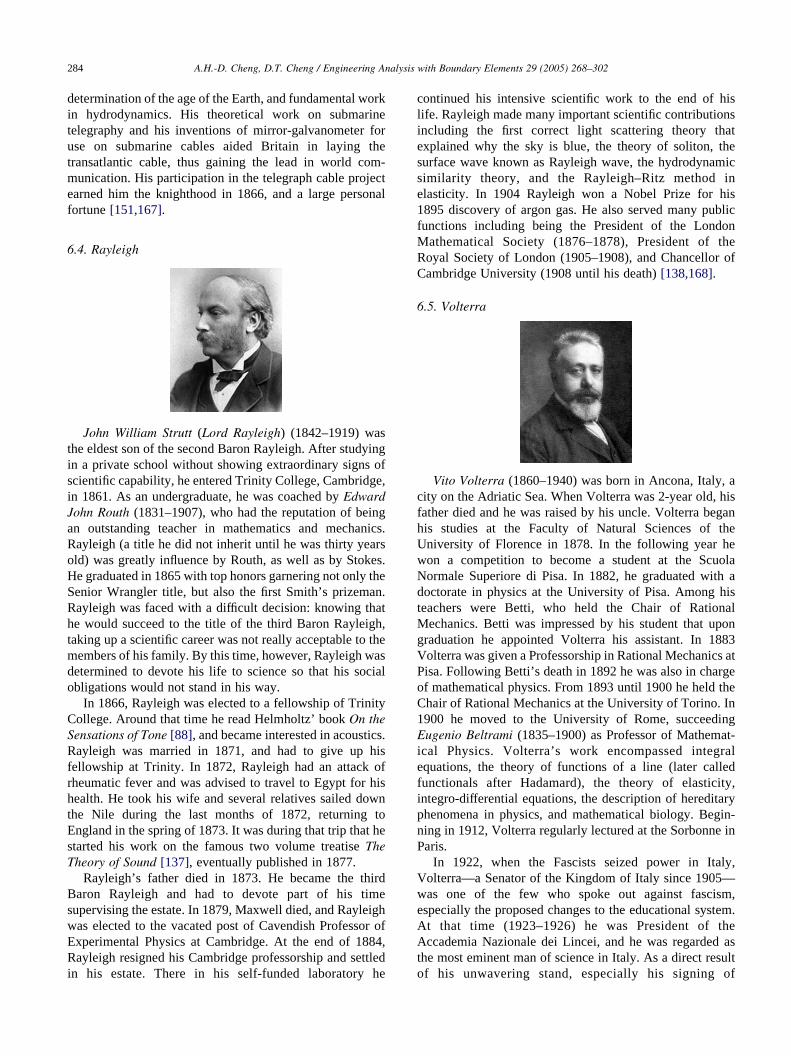
A.H.-D. Cheng, D.T. Cheng / Engineering Analysis with Boundary Elements 29 (2005) 268–302284

determination of the age of the Earth, and fundamental work

in hydrodynamics. His theoretical work on submarine

telegraphy and his inventions of mirror-galvanometer for

use on submarine cables aided Britain in laying the

transatlantic cable, thus gaining the lead in world com-

munication. His participation in the telegraph cable project

earned him the knighthood in 1866, and a large personal

fortune [151,167].

6.4. Rayleigh

John William Strutt (Lord Rayleigh) (1842–1919) was

the eldest son of the second Baron Rayleigh. After studying

in a private school without showing extraordinary signs of

scientific capability, he entered Trinity College, Cambridge,

in 1861. As an undergraduate, he was coached by Edward

John Routh (1831–1907), who had the reputation of being

an outstanding teacher in mathematics and mechanics.

Rayleigh (a title he did not inherit until he was thirty years

old) was greatly influence by Routh, as well as by Stokes.

He graduated in 1865 with top honors garnering not only the

Senior Wrangler title, but also the first Smith’s prizeman.

Rayleigh was faced with a difficult decision: knowing that

he would succeed to the title of the third Baron Rayleigh,

taking up a scientific career was not really acceptable to the

members of his family. By this time, however, Rayleigh was

determined to devote his life to science so that his social

obligations would not stand in his way.

In 1866, Rayleigh was elected to a fellowship of Trinity

College. Around that time he read Helmholtz’ book On the

Sensations of Tone [88], and became interested in acoustics.

Rayleigh was married in 1871, and had to give up his

fellowship at Trinity. In 1872, Rayleigh had an attack of

rheumatic fever and was advised to travel to Egypt for his

health. He took his wife and several relatives sailed down

the Nile during the last months of 1872, returning to

England in the spring of 1873. It was during that trip that he

started his work on the famous two volume treatise The

Theory of Sound [137], eventually published in 1877.

Rayleigh’s father died in 1873. He became the third

Baron Rayleigh and had to devote part of his time

supervising the estate. In 1879, Maxwell died, and Rayleigh

was elected to the vacated post of Cavendish Professor of

Experimental Physics at Cambridge. At the end of 1884,

Rayleigh resigned his Cambridge professorship and settled

in his estate. There in his self-funded laboratory he

continued his intensive scientific work to the end of his

life. Rayleigh made many important scientific contributions

including the first correct light scattering theory that

explained why the sky is blue, the theory of soliton, the

surface wave known as Rayleigh wave, the hydrodynamic

similarity theory, and the Rayleigh–Ritz method in

elasticity. In 1904 Rayleigh won a Nobel Prize for his

1895 discovery of argon gas. He also served many public

functions including being the President of the London

Mathematical Society (1876–1878), President of the

Royal Society of London (1905–1908), and Chancellor of

Cambridge University (1908 until his death) [138,168].

6.5. Volterra

Vito Volterra (1860–1940) was born in Ancona, Italy, a

city on the Adriatic Sea. When Volterra was 2-year old, his

father died and he was raised by his uncle. Volterra began

his studies at the Faculty of Natural Sciences of the

University of Florence in 1878. In the following year he

won a competition to become a student at the Scuola

Normale Superiore di Pisa. In 1882, he graduated with a

doctorate in physics at the University of Pisa. Among his

teachers were Betti, who held the Chair of Rational

Mechanics. Betti was impressed by his student that upon

graduation he appointed Volterra his assistant. In 1883

Volterra was given a Professorship in Rational Mechanics at

Pisa. Following Betti’s death in 1892 he was also in charge

of mathematical physics. From 1893 until 1900 he held the

Chair of Rational Mechanics at the University of Torino. In

1900 he moved to the University of Rome, succeeding

Eugenio Beltrami (1835–1900) as Professor of Mathemat-

ical Physics. Volterra’s work encompassed integral

equations, the theory of functions of a line (later called

functionals after Hadamard), the theory of elasticity,

integro-differential equations, the description of hereditary

phenomena in physics, and mathematical biology. Begin-

ning in 1912, Volterra regularly lectured at the Sorbonne in

Paris.

In 1922, when the Fascists seized power in Italy,

Volterra—a Senator of the Kingdom of Italy since 1905—

was one of the few who spoke out against fascism,

especially the proposed changes to the educational system.

At that time (1923–1926) he was President of the

Accademia Nazionale dei Lincei, and he was regarded as

the most eminent man of science in Italy. As a direct result

of his unwavering stand, especially his signing of

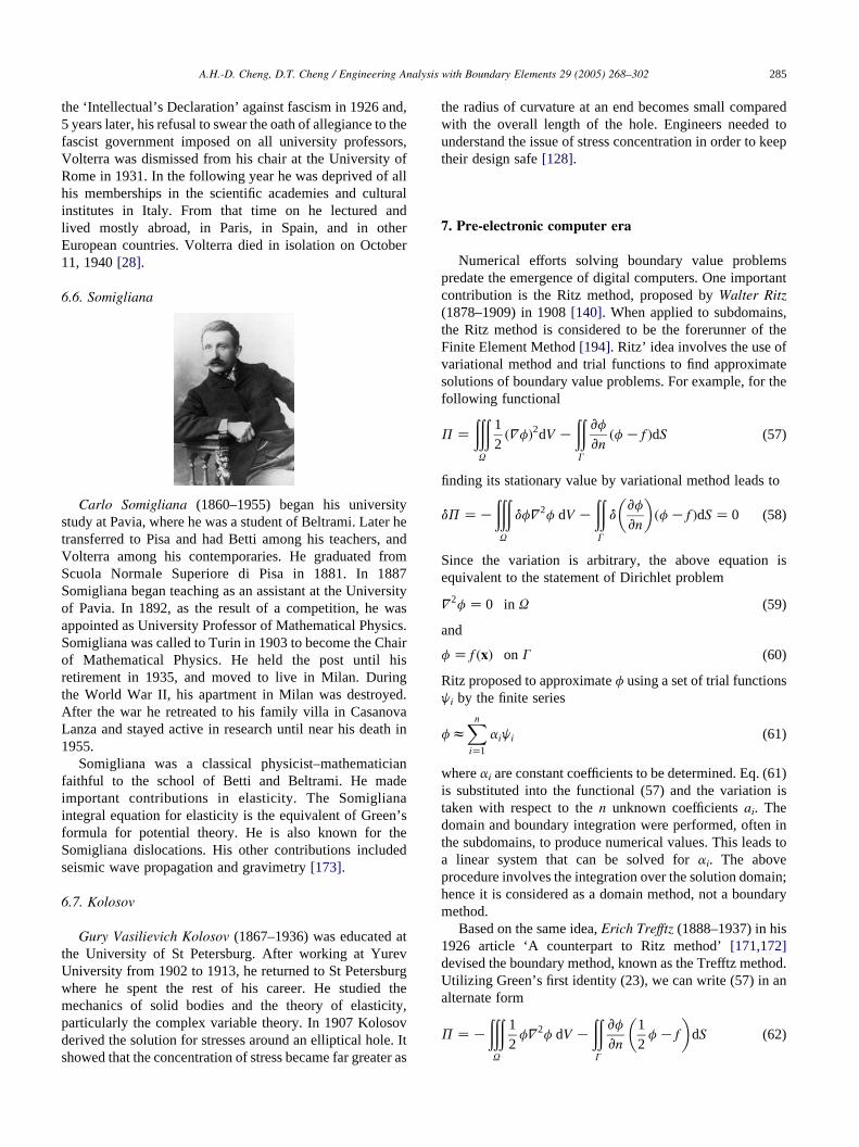
A.H.-D. Cheng, D.T. Cheng / Engineering Analysis with Boundary Elements 29 (2005) 268–302 285

the ‘Intellectual’s Declaration’ against fascism in 1926 and,

5 years later, his refusal to swear the oath of allegiance to the

fascist government imposed on all university professors,

Volterra was dismissed from his chair at the University of

Rome in 1931. In the following year he was deprived of all

his memberships in the scientific academies and cultural

institutes in Italy. From that time on he lectured and

lived mostly abroad, in Paris, in Spain, and in other

European countries. Volterra died in isolation on October

11, 1940 [28].

6.6. Somigliana

Carlo Somigliana (1860–1955) began his university

study at Pavia, where he was a student of Beltrami. Later he

transferred to Pisa and had Betti among his teachers, and

Volterra among his contemporaries. He graduated from

Scuola Normale Superiore di Pisa in 1881. In 1887

Somigliana began teaching as an assistant at the University

of Pavia. In 1892, as the result of a competition, he was

appointed as University Professor of Mathematical Physics.

Somigliana was called to Turin in 1903 to become the Chair

of Mathematical Physics. He held the post until his

retirement in 1935, and moved to live in Milan. During

the World War II, his apartment in Milan was destroyed.

After the war he retreated to his family villa in Casanova

Lanza and stayed active in research until near his death in

1955.

Somigliana was a classical physicist–mathematician

faithful to the school of Betti and Beltrami. He made

important contributions in elasticity. The Somigliana

integral equation for elasticity is the equivalent of Green’s

formula for potential theory. He is also known for the

Somigliana dislocations. His other contributions included

seismic wave propagation and gravimetry [173].

6.7. Kolosov

Gury Vasilievich Kolosov (1867–1936) was educated at

the University of St Petersburg. After working at Yurev

University from 1902 to 1913, he returned to St Petersburg

where he spent the rest of his career. He studied the

mechanics of solid bodies and the theory of elasticity,

particularly the complex variable theory. In 1907 Kolosov

derived the solution for stresses around an elliptical hole. It

showed that the concentration of stress became far greater as

the radius of curvature at an end becomes small compared

with the overall length of the hole. Engineers needed to

understand the issue of stress concentration in order to keep

their design safe [128].

7. Pre-electronic computer era

Numerical efforts solving boundary value problems

predate the emergence of digital computers. One important

contribution is the Ritz method, proposed by Walter Ritz

(1878–1909) in 1908 [140]. When applied to subdomains,

the Ritz method is considered to be the forerunner of the

Finite Element Method [194]. Ritz’ idea involves the use of

variational method and trial functions to find approximate

solutions of boundary value problems. For example, for the

following functional

P Z

ðððU

1

2ðVfÞ2dV K

ððG

vf

vnðf K f ÞdS (57)

finding its stationary value by variational method leads to

dP ZK

ðððU

dfV2f dV K

ððG

dvf

vn

� �ðf K f ÞdS Z 0 (58)

Since the variation is arbitrary, the above equation is

equivalent to the statement of Dirichlet problem

V2f Z 0 in U (59)

and

f Z f ðxÞ on G (60)

Ritz proposed to approximate f using a set of trial functions

ji by the finite series

fzXn

iZ1

aiji (61)

where ai are constant coefficients to be determined. Eq. (61)

is substituted into the functional (57) and the variation is

taken with respect to the n unknown coefficients ai. The

domain and boundary integration were performed, often in

the subdomains, to produce numerical values. This leads to

a linear system that can be solved for ai. The above

procedure involves the integration over the solution domain;

hence it is considered as a domain method, not a boundary

method.

Based on the same idea, Erich Trefftz (1888–1937) in his

1926 article ‘A counterpart to Ritz method’ [171,172]

devised the boundary method, known as the Trefftz method.

Utilizing Green’s first identity (23), we can write (57) in an

alternate form

P ZK

ðððU

1

2fV2f dV K

ððG

vf

vn

1

2f K f

� �dS (62)

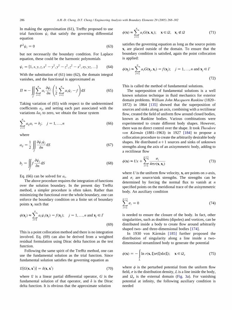
A.H.-D. Cheng, D.T. Cheng / Engineering Analysis with Boundary Elements 29 (2005) 268–302286

In making the approximation (61), Trefftz proposed to use

trial functions ji that satisfy the governing differential

equation

V2ji Z 0 (63)

but not necessarily the boundary condition. For Laplace

equation, these could be the harmonic polynomials

ji Z f1; x; y; z; x2 Ky2; y2 Kz2; z2 Kx2; xy; yz;.g (64)

With the substitution of (61) into (62), the domain integral

vanishes, and the functional is approximated as

PzK

ððG

Xn

iZ1

ai

vji

vn

1

2

Xn

iZ1

aiji K f

!dS (65)

Taking variation of (65) with respect to the undetermined

coefficients aj, and setting each part associated with the

variations daj to zero, we obtain the linear system

Xn

iZ1

aijai Z bj; j Z 1;.; n (66)

where

aij Z1

2

ððG

vjijj

vndS (67)

bj Z

ððG

fvjj

vndS (68)

Eq. (66) can be solved for ai.

The above procedure requires the integration of functions

over the solution boundary. In the present day Trefftz

method, a simpler procedure is often taken. Rather than

minimizing the functional over the whole boundary, one can

enforce the boundary condition on a finite set of boundary

points xj such that

fðxjÞzXn

iZ1

aijiðxjÞ Z f ðxjÞ; j Z 1;.; n and xj 2G

(69)

This is a point collocation method and there is no integration

involved. Eq. (69) can also be derived from a weighted

residual formulation using Dirac delta function as the test

function.

Following the same spirit of the Trefftz method, one can

use the fundamental solution as the trial function. Since

fundamental solution satisfies the governing equation as

LfGðx; x0Þg Z dðx; x0Þ (70)

where L is a linear partial differential operator, G is the

fundamental solution of that operator, and d is the Dirac

delta function. It is obvious that the approximate solution

fðxÞzXn

iZ1

aiGðx; xiÞ; x2U; xi ;U (71)

satisfies the governing equation as long as the source points

xi are placed outside of the domain. To ensure that the

boundary condition is satisfied, again the point collocation

is applied:

fðxjÞzXn

iZ1

aiGðxj; xiÞ Z f ðxjÞ; j Z 1;.; n and xj 2G

(72)

This is called the method of fundamental solutions.

The superposition of fundamental solutions is a well

known solution technique in fluid mechanics for exterior

domain problems. William John Macquorn Rankine (1820–

1872) in 1864 [135] showed that the superposition of

sources and sinks along an axis, combining with a rectilinear

flow, created the field of uniform flow around closed bodies,

known as Rankine bodies. Various combinations were

experimented to create different body shapes. However,

there was no direct control over the shape. It took Theodore

von Karman (1881–1963) in 1927 [184] to propose a

collocation procedure to create the arbitrarily desirable body

shapes. He distributed nC1 sources and sinks of unknown

strengths along the axis of an axisymmetric body, adding to

a rectilinear flow

fðxÞzUx CXnC1

iZ1

si

4prðx; xiÞ(73)

where U is the uniform flow velocity, xi are points on x-axis,

and si are source/sink strengths. The strengths can be

determined by forcing the normal flux to vanish at n

specified points on the meridional trace of the axisymmetric

body. An auxiliary condition

XnC1

iZ1

si Z 0 (74)

is needed to ensure the closure of the body. In fact, other

singularities, such as doublets (dipoles) and vortices, can be

distributed inside a body to create flow around arbitrarily

shaped two- and three-dimensional bodies [174].

In 1930 von Karman [185] further proposed the

distribution of singularity along a line inside a two-

dimensional streamlined body to generate the potential

fðxÞ ZK

ðL

ln rðx; xÞsðxÞdsðxÞ; x2Ue (75)

where f is the perturbed potential from the uniform flow

field, s is the distribution density, L is a line inside the body,

and Ue is the external domain (Fig. 3a). For vanishing

potential at infinity, the following auxiliary condition is

needed

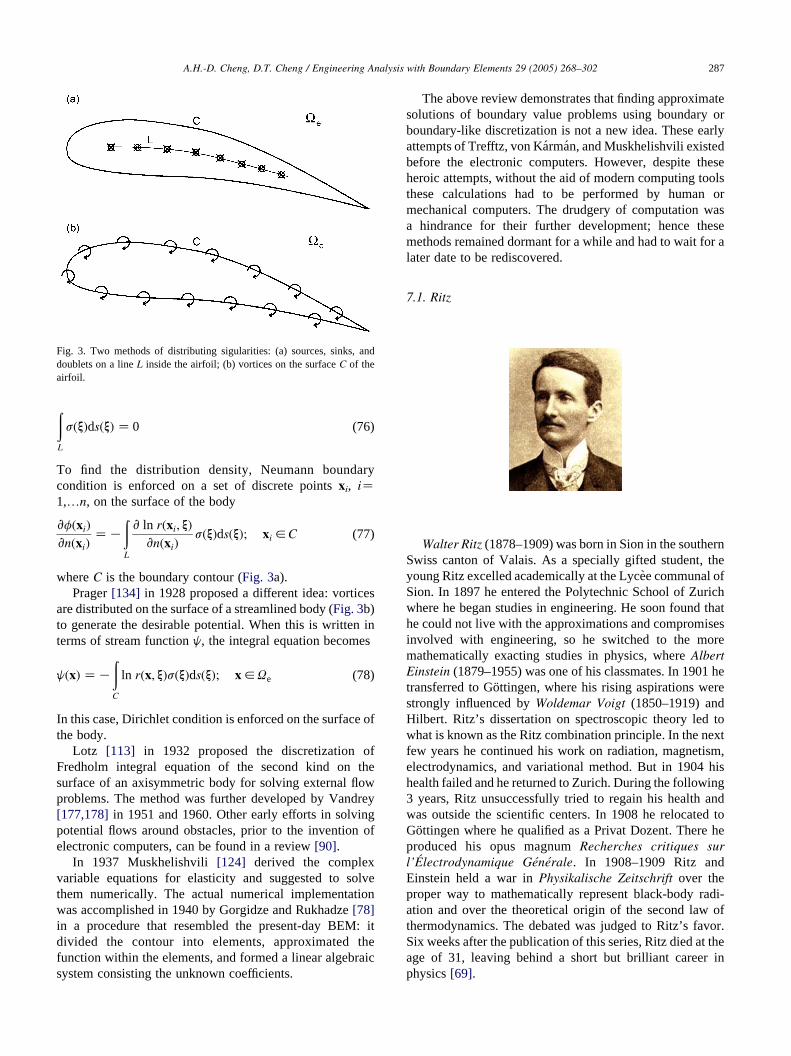
Fig. 3. Two methods of distributing sigularities: (a) sources, sinks, and

doublets on a line L inside the airfoil; (b) vortices on the surface C of the

airfoil.

A.H.-D. Cheng, D.T. Cheng / Engineering Analysis with Boundary Elements 29 (2005) 268–302 287

ðL

sðxÞdsðxÞ Z 0 (76)

To find the distribution density, Neumann boundary

condition is enforced on a set of discrete points xi, iZ1,.n, on the surface of the body

vfðxiÞ

vnðxiÞZK

ðL

v ln rðxi; xÞ

vnðxiÞsðxÞdsðxÞ; xi 2C (77)

where C is the boundary contour (Fig. 3a).

Prager [134] in 1928 proposed a different idea: vortices

are distributed on the surface of a streamlined body (Fig. 3b)

to generate the desirable potential. When this is written in

terms of stream function j, the integral equation becomes

jðxÞ ZK

ðC

ln rðx; xÞsðxÞdsðxÞ; x2Ue (78)

In this case, Dirichlet condition is enforced on the surface of

the body.

Lotz [113] in 1932 proposed the discretization of

Fredholm integral equation of the second kind on the

surface of an axisymmetric body for solving external flow

problems. The method was further developed by Vandrey

[177,178] in 1951 and 1960. Other early efforts in solving

potential flows around obstacles, prior to the invention of

electronic computers, can be found in a review [90].

In 1937 Muskhelishvili [124] derived the complex

variable equations for elasticity and suggested to solve

them numerically. The actual numerical implementation

was accomplished in 1940 by Gorgidze and Rukhadze [78]

in a procedure that resembled the present-day BEM: it

divided the contour into elements, approximated the

function within the elements, and formed a linear algebraic

system consisting the unknown coefficients.

The above review demonstrates that finding approximate

solutions of boundary value problems using boundary or

boundary-like discretization is not a new idea. These early

attempts of Trefftz, von Karman, and Muskhelishvili existed

before the electronic computers. However, despite these

heroic attempts, without the aid of modern computing tools

these calculations had to be performed by human or

mechanical computers. The drudgery of computation was

a hindrance for their further development; hence these

methods remained dormant for a while and had to wait for a

later date to be rediscovered.

7.1. Ritz

Walter Ritz (1878–1909) was born in Sion in the southern

Swiss canton of Valais. As a specially gifted student, the

young Ritz excelled academically at the Lycee communal of

Sion. In 1897 he entered the Polytechnic School of Zurich

where he began studies in engineering. He soon found that

he could not live with the approximations and compromises

involved with engineering, so he switched to the more

mathematically exacting studies in physics, where Albert

Einstein (1879–1955) was one of his classmates. In 1901 he

transferred to Gottingen, where his rising aspirations were

strongly influenced by Woldemar Voigt (1850–1919) and

Hilbert. Ritz’s dissertation on spectroscopic theory led to

what is known as the Ritz combination principle. In the next

few years he continued his work on radiation, magnetism,

electrodynamics, and variational method. But in 1904 his

health failed and he returned to Zurich. During the following

3 years, Ritz unsuccessfully tried to regain his health and

was outside the scientific centers. In 1908 he relocated to

Gottingen where he qualified as a Privat Dozent. There he

produced his opus magnum Recherches critiques sur

l’Electrodynamique Generale. In 1908–1909 Ritz and

Einstein held a war in Physikalische Zeitschrift over the

proper way to mathematically represent black-body radi-

ation and over the theoretical origin of the second law of

thermodynamics. The debated was judged to Ritz’s favor.

Six weeks after the publication of this series, Ritz died at the

age of 31, leaving behind a short but brilliant career in

physics [69].

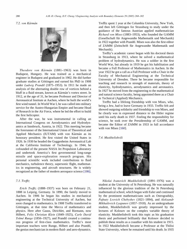
A.H.-D. Cheng, D.T. Cheng / Engineering Analysis with Boundary Elements 29 (2005) 268–302288

7.2. von Karman

Theodore von Karman (1881–1963) was born in

Budapest, Hungary. He was trained as a mechanical

engineer in Budapest and graduated in 1902. He did further

graduate studies at Gottingen and earned his PhD in 1908

under Ludwig Prandtl (1875–1953). In 1911 he made an

analysis of the alternating double row of vortices behind a

bluff in a fluid stream, known as Karman’s vortex street. In

1912, at the age of 31, he became Professor and Director of

Aeronautical Institute at Aachen, where he built the world’s

first wind tunnel. In World War I, he was called into military

service for the Austro-Hungarian Empire and became Head

of Research in the Air Force, where he led the effort to build

the first helicopter.

After the war, he was instrumental in calling an

International Congress on Aerodynamics and Hydrodyn-

amics at Innsbruck, Austria, in 1922. This meeting became

the forerunner of the International Union of Theoretical and

Applied Mechanics (IUTAM) with von Karman as its

honorary president. He first visited the United States in

1926. In 1930 he headed the Guggenheim Aeronautical Lab

at the California Institute of Technology. In 1944, he

cofounded of the present NASA Jet Propulsion Laboratory

and undertook America’s first governmental long-range

missile and space-exploration research program. His

personal scientific work included contributions to fluid

mechanics, turbulence theory, supersonic flight, mathemat-

ics in engineering, and aircraft structures. He is widely

recognized as the father of modern aerospace science [186].

7.3. Trefftz

Erich Trefftz (1888–1937) was born on February 21,

1888 in Leipzig, Germany. In 1890, the family moved to

Aachen. In 1906 he began his studies in mechanical

engineering at the Technical University of Aachen, but

soon changed to mathematics. In 1908 Trefftz transferred to

Gottingen, at that time the Mecca of mathematics and

physics. Here after Gauss, Dirichlet, and Riemann, now

Hilbert, Felix Christian Klein (1849–1925), Carle David

Tolme Runge (1856–1927), and Prandtl created a continu-

ous progress of first-class mathematics. Trefftz’s most

important teachers were Runge, Hilbert and also Prandtl,

the genius mechanician in modern fluid- and aero-dynamics.

Trefftz spent 1 year at the Columbia University, New York,

and then left Gottingen for Strassburg to study under the

guidance of the famous Austrian applied mathematician

Richard von Mises (1883–1953), who founded the GAMM

(Gesellschaft fur Angewandte Mathematik und Mechanik)

in 1922 together with Prandtl. Mises was also the first editor

of ZAMM (Zeitschrift fur Angewandte Mathematik und

Mechanik).

Trefftz’s academic career began with his doctoral thesis

in Strassburg in 1913, where he solved a mathematical

problem of hydrodynamics. He was a soldier in the first

World War, but already in 1919 he got his habilitation and

became a Full Professor of Mathematics in Aachen. In the

year 1922 he got a call as a Full Professor with a Chair in the

Faculty of Mechanical Engineering at the Technical

University of Dresden. There he became responsible for

teaching and research in strength of materials, theory of

elasticity, hydrodynamics, aerodynamics and aeronautics.

In 1927 he moved from the engineering to the mathematical

and natural science faculty, being appointed there as a Chair

in Technical (Applied) Mechanics.

Trefftz had a lifelong friendship with von Mises, who,

being a Jew, had to leave Germany in 1933. Trefftz felt and

showed outgoing solidarity and friendship to von Mises, and

he clearly was in expressed distance to the Hitler regime

until his early death in 1937. Feeling the responsibility for

science, he took over the Presidentship of GAMM, and

became the Editor of ZAMM in 1933 in full accordance

with von Mises [160].

7.4. Muskhelishvili

Nikolai Ivanovich Muskhelishvili (1891–1976) was a

student at the University of St Petersburg. He was naturally

influenced by the glorious tradition of the St Petersburg

mathematical school, which began with Euler and continued

by the prominent mathematicians such as Ostrogradsky,

Pafnuty Lvovich Chebyshev (1821–1894), and Aleksandr

Mikhailovich Lyapunov (1857–1918). As an undergraduate

student, Muskhelishvili was greatly impressed by the

lectures of Kolosov on the complex variable theory of

elasticity. Muskhelishvili took this topic as his graduation

thesis and performed brilliantly that Kolosov decided to

publish these results as a coauthor with his student in 1915.

In 1922 Muskhelishvili became a Professor at the Tbilisi

State University, where he remained until his death. In 1935

A.H.-D. Cheng, D.T. Cheng / Engineering Analysis with Boundary Elements 29 (2005) 268–302 289

he published the masterpiece Some Basic Problems of the

Mathematical Theory of Elasticity, which won him the

Stalin Prize of the First Degree. He held many positions

such as Chair, Director, President, at Tbilisi and the

Georgian Branch of USSR Academy of Sciences, and

received many honors [196,197].

8. Electronic computer era

Although electronic computers were invented in the

1940s, they did not become widely available to common

researchers until the early 1960s. It is not surprising that the

development of the finite element method [38], as well as a

number of other numerical methods, started around that

time. A number of independent efforts of experimenting on

boundary methods also emerged in the early 1960s. Some of

the more significant ones are reviewed below.

Friedman and Shaw [68] in 1962 solved the scalar wave

equation

V2f K1

c2

v2f

vt2Z 0 (79)

in the time domain for the scattered wave field resulting

from a shock wave impinging on a cylindrical obstacle. In

the above f is the velocity potential and c is the wave speed.

The use of the fundamental solution

G ZK1

rd

r

cK ðt K t0Þ

h i(80)

where d is the Dirac delta function, in Green’s second

identity (24) produced the boundary integral equation

fscðx; tÞ Z1

4p

ðtC

0

ððG

Gvfsc

vnKfsc

vG

vn

� �dS dt0 (81)

where fsc is the scattered wave field. Eq. (81) was further

differentiated with respect to time to create the equation for

acoustic pressure. For a two-dimensional problem, the

equation was discretized in space (boundary contour) and in

time that resulted into a double summation. Variables were

assumed to be constant over space and time subintervals, so

the integration could be performed exactly. Finite difference

explicit time-stepping scheme was used and the resultant

algebraic system required only successive, not simultaneous

solution. The computation was carried out using a Monroe

desk calculator [154]. The scattering due to a box-shaped

rigid obstacle was solved. The work was extended in 1967

by Shaw [152] to handle different boundary conditions on

the obstacle surface, and by Mitzner [122] using the retarded

potential integral representation.

Banaugh and Goldsmith [5] in 1963 tackled the two-

dimensional wave equation in the frequency domain,

governed by the Helmholtz equation (38). The 2-D boundary

integral equation counterpart to the 3-D version (40) is

f Zi

4

ðC

Hð1Þ0 ðkrÞ

vf

vnKf

vHð1Þ0 ðkrÞ

vn

" #ds (82)

where Hð1Þ0 is the Hankel function of the first kind of order

zero, k is the wave number, and iZffiffiffiffiffiffiK1

p. Eq. (82) is solved in

the complex variable domain. Similar to Friedman and Shaw

[68], the integration over a subinterval was made easy by

assuming constant variation of the potential on the

subinterval. The problem of a steady state wave scattered

from the surface of a circular cylinder was solved as a

demonstration. An IBM 7090 mainframe computer was used

for the numerical solution. It is of interest to observe that the

discretization was restricted to 36 points, corresponding to 72

unknowns (real and imaginary parts), due to the memory

restriction of the computer. A larger linear system would

have required the read/write operation on the tape storage and

special linear system solution algorithm.

In the same year (1963) Chen and Schweikert [36] solved

the three-dimensional sound radiation problem in the

frequency domain using the Fredholm integral equation of

the second kind

vfðxÞ

vnðxÞZK2psðxÞC

ððG

sðxÞv

vnðxÞ

eikr

r

� �dSðxÞ; x2G

(83)

Problems of vibrating spherical and cylindrical shells in

infinite fluid domain were solved. The surface was divided

into triangular elements. An IBM 704 mainframe was used,

which allowed up to 1000 degrees of freedom to be

modeled.

Subsequent work using integral equation solving acous-

tic scattering problems included Chertock [37] in 1964, and

Copley in 1967 [40] and 1968 [41]. Copley was the first to

report the non-uniqueness of integral equation formulation

due to the existence of eigen frequencies. Schenck [150] in

1968 presented the CHIEF (combined Helmholtz integral

equation formulation). Waterman developed the null-field

and T-matrix method, first in 1965 [188] for solving

electromagnetic scattering problems, and then in 1969

[189] for acoustic problems. In both the CHIEF and the

T-matrix method, the so-called ‘null-field integral equation’

or the ‘interior Helmholtz integral equation’ was utilized:

0 Z

ððG

fðxÞvGðx; xÞ

vnðxÞKGðx; xÞ

vfðxÞ

vnðxÞdSðxÞ; x2Ui (84)

where Ui is the interior of the scatterer, and

G ZK1

4preKikr (85)

is the free-space Green’s function of Helmholtz equation.

The left hand side of (84) is null because the source point x

is placed inside the body, which is outside the wave field.

The above equation was combined with the exterior integral

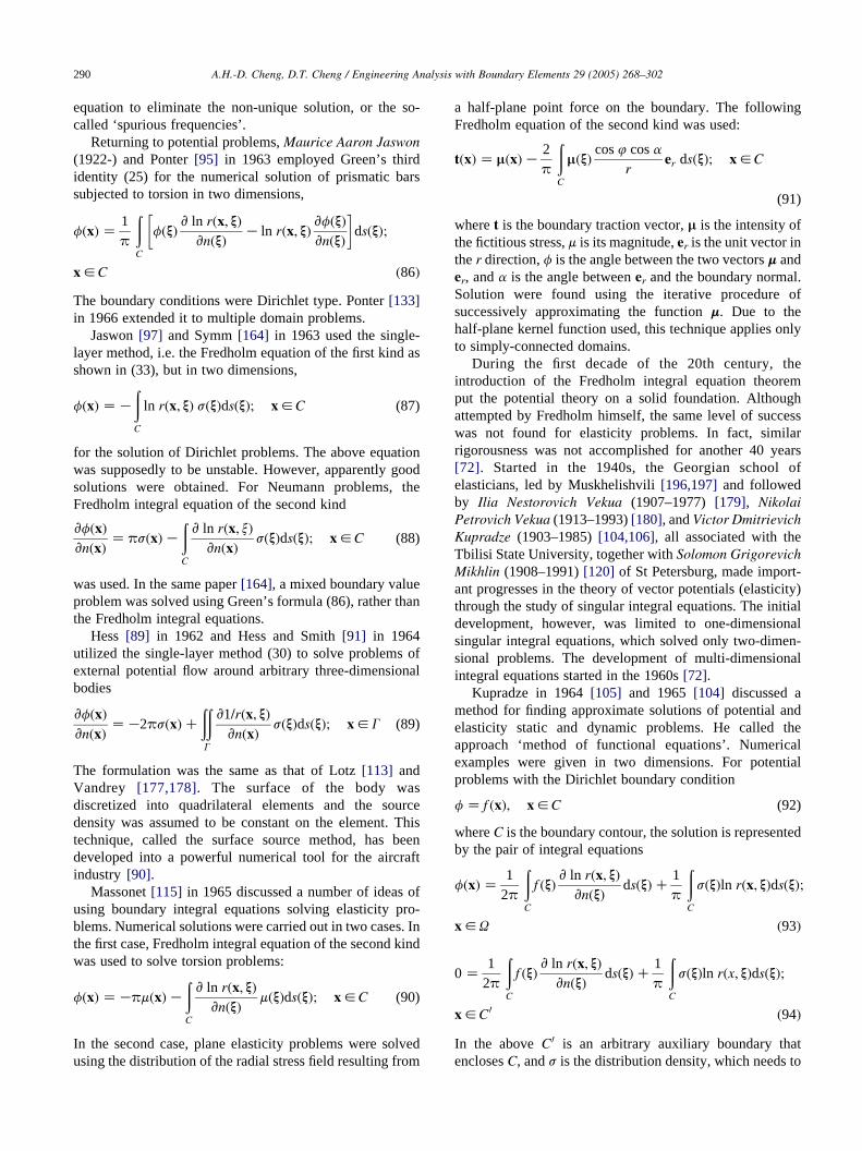
A.H.-D. Cheng, D.T. Cheng / Engineering Analysis with Boundary Elements 29 (2005) 268–302290

equation to eliminate the non-unique solution, or the so-

called ‘spurious frequencies’.

Returning to potential problems, Maurice Aaron Jaswon

(1922-) and Ponter [95] in 1963 employed Green’s third

identity (25) for the numerical solution of prismatic bars

subjected to torsion in two dimensions,

fðxÞ Z1

p

ðC

fðxÞv ln rðx; xÞ

vnðxÞK ln rðx; xÞ

vfðxÞ

vnðxÞ

� �dsðxÞ;

x2C ð86Þ

The boundary conditions were Dirichlet type. Ponter [133]

in 1966 extended it to multiple domain problems.

Jaswon [97] and Symm [164] in 1963 used the single-

layer method, i.e. the Fredholm equation of the first kind as

shown in (33), but in two dimensions,

fðxÞ ZK

ðC

ln rðx; xÞ sðxÞdsðxÞ; x2C (87)

for the solution of Dirichlet problems. The above equation

was supposedly to be unstable. However, apparently good

solutions were obtained. For Neumann problems, the

Fredholm integral equation of the second kind

vfðxÞ

vnðxÞZ psðxÞK

ðC

v ln rðx; xÞ

vnðxÞsðxÞdsðxÞ; x2C (88)

was used. In the same paper [164], a mixed boundary value

problem was solved using Green’s formula (86), rather than

the Fredholm integral equations.

Hess [89] in 1962 and Hess and Smith [91] in 1964

utilized the single-layer method (30) to solve problems of

external potential flow around arbitrary three-dimensional

bodies

vfðxÞ

vnðxÞZK2psðxÞC

ððG

v1=rðx; xÞ

vnðxÞsðxÞdsðxÞ; x2G (89)

The formulation was the same as that of Lotz [113] and

Vandrey [177,178]. The surface of the body was

discretized into quadrilateral elements and the source

density was assumed to be constant on the element. This

technique, called the surface source method, has been

developed into a powerful numerical tool for the aircraft

industry [90].

Massonet [115] in 1965 discussed a number of ideas of

using boundary integral equations solving elasticity pro-

blems. Numerical solutions were carried out in two cases. In

the first case, Fredholm integral equation of the second kind

was used to solve torsion problems:

fðxÞ ZKpmðxÞK

ðC

v ln rðx; xÞ

vnðxÞmðxÞdsðxÞ; x2C (90)

In the second case, plane elasticity problems were solved

using the distribution of the radial stress field resulting from

a half-plane point force on the boundary. The following

Fredholm equation of the second kind was used:

tðxÞ Z mðxÞK2

p

ðC

mðxÞcos 4 cos a

rer dsðxÞ; x2C

(91)

where t is the boundary traction vector, m is the intensity of

the fictitious stress, m is its magnitude, er is the unit vector in

the r direction, f is the angle between the two vectors m and

er, and a is the angle between er and the boundary normal.

Solution were found using the iterative procedure of

successively approximating the function m. Due to the

half-plane kernel function used, this technique applies only

to simply-connected domains.

During the first decade of the 20th century, the

introduction of the Fredholm integral equation theorem

put the potential theory on a solid foundation. Although

attempted by Fredholm himself, the same level of success

was not found for elasticity problems. In fact, similar

rigorousness was not accomplished for another 40 years

[72]. Started in the 1940s, the Georgian school of

elasticians, led by Muskhelishvili [196,197] and followed

by Ilia Nestorovich Vekua (1907–1977) [179], Nikolai

Petrovich Vekua (1913–1993) [180], and Victor Dmitrievich

Kupradze (1903–1985) [104,106], all associated with the

Tbilisi State University, together with Solomon Grigorevich

Mikhlin (1908–1991) [120] of St Petersburg, made import-

ant progresses in the theory of vector potentials (elasticity)

through the study of singular integral equations. The initial

development, however, was limited to one-dimensional

singular integral equations, which solved only two-dimen-

sional problems. The development of multi-dimensional

integral equations started in the 1960s [72].

Kupradze in 1964 [105] and 1965 [104] discussed a

method for finding approximate solutions of potential and

elasticity static and dynamic problems. He called the

approach ‘method of functional equations’. Numerical

examples were given in two dimensions. For potential

problems with the Dirichlet boundary condition

f Z f ðxÞ; x2C (92)

where C is the boundary contour, the solution is represented

by the pair of integral equations

fðxÞ Z1

2p

ðC

f ðxÞv ln rðx; xÞ

vnðxÞdsðxÞC

1

p

ðC

sðxÞln rðx; xÞdsðxÞ;

x2U ð93Þ

0 Z1

2p

ðC

f ðxÞv ln rðx; xÞ

vnðxÞdsðxÞC

1

p

ðC

sðxÞln rðx; xÞdsðxÞ;

x2C 0 ð94Þ

In the above C 0 is an arbitrary auxiliary boundary that

encloses C, and s is the distribution density, which needs to

A.H.-D. Cheng, D.T. Cheng / Engineering Analysis with Boundary Elements 29 (2005) 268–302 291

be solved from (94). We notice that the above equations

involve the distribution of both the single-layer and the

double-layer potential. Another observation is that in (94) the

center of singularity x is located on C 0, which is outside of the

solution domain U. Since C and C 0 are distinct contours, Eq.

(94) is not an integral equation in the classical sense, in which

the singularities are located on the boundary. This is why the

term ‘functional equation’ was used instead. In the numerical

implementation, C 0 was chosen as a circles, upon which n

nodes were selected to place the singularity. Since the

singularities were not located on the boundary C, the

integrals in (94) were regular and could be numerically

evaluated using a simple quadrature rule. Gaussian quad-

rature with n nodes was used for the integration. The resultant

linear system was solved for the n discrete s values located at

the quadrature nodes. Eq. (93) was then used to find solution

at any point in the domain.

For elasticity problems, the same technique was

employed. For static, two-dimensional problems with

prescribed boundary displacement

ui Z fiðxÞ; x2C (95)

the following pair of vector integral equations solve the

boundary value problem:

ujðxÞ Z1

p

ðC

siðxÞufijðx; xÞdsðxÞK

1

2p

ðC

fiðxÞudijðx; xÞdsðxÞ;

x2U ð96Þ

0 Z1

p

ðC

siðxÞufijðx; xÞdsðxÞK

1

2p

ðC

fiðxÞudijðx; xÞdsðxÞ;

x2C 0 ð97Þ

where si is the distribution density (vector), and the kernel

ufij Z

1

4Gð1 KnÞð3 K4nÞdij ln r K

xixj

r2

h i(98)

is the fundamental solution due to a point force (single-layer

potential) in the xj direction, and

udij Z

1

2ð1 KnÞ

!1

rð1 K2nÞ

nixj

rK

njxi

rCdij

vr

vn

� �C2

xixj

r2

vr

vn

� �(99)

is the fundamental solution due to a dislocation (double-

layer potential) oriented in the xj direction. Kupradze’s

method was closely followed in Russia under the name

‘potential method’, particularly in the solution of shells [71,

176] and plates [103,181].

Kupradze’s technique of distributing fundamental sol-

utions on an exterior, auxiliary boundary has been

considered by some as the origin of the ‘method of

fundamental solutions’ [14]. However, in most applications

[65], the method of fundamental solutions often bypasses

the integral equation formulation. It considers the distri-

bution of admissible solutions of discrete and unknown

density on an external auxiliary boundary, for example, in

the form of (71). The boundary conditions are satisfied by

collocating at a set of boundary nodes. Hence the method of

fundamental solutions, although can be viewed as a special

case of the method of functional equations, was in

fact independently developed. For example, Oliveira [130]

in 1968 proposed the use of fundamental solution of

point forces linearly distributed over linear segments to

solve plane elasticity problems. For potential problems,

the recent origin can be traced to Mathon and Johnston [116]

in 1977.

Another type of problems that has traditionally used

boundary methods involves problems with discontinuities

such as fractures, dislocations resulting from imperfec-

tions of crystalline structures, interface between dissim-

ilar materials, and other discontinuities. In these cases,

certain physical quantities, such as displacements or

stresses, suffer a jump. These discontinuities can be

simulated by the distribution of singular solutions such

as the Volterra [183] and Somigliana dislocations [158,

159] over the physical surface, which often results in

integral equations [12,62]. For example, integral

equation of this type

AðxÞjðxÞC1

p

ðb

a

Bðx0Þjðx0Þ

x0 Kxdx0 C

ðb

aKðx; x0Þjðx0Þdx0 Z f ðxÞ;

a!x!b ð100Þ

and other types were numerically investigated by

Erdogan and Gupta [60,61] in 1972 using Chebyshev

and Jacobi polynomials for the approximation. These

type of one-dimensional singular integral equations has

also been solved using piece-wise, low degree poly-

nomials [74].

The review presented so far has focused on the solution

of physical and engineering problems. The formulations

often borrow the physical idea of distributing concentrated

loads; hence the integral equations are typically singular.

Due to the existence of multiple spatial and the time

dimensions in physical problems, the integral equations are

often multi-dimensional.

For the mathematical community, the effort of finding

approximate solutions of integral equations existed since the

major breakthrough of Fredholm in the 1900s. Early efforts

focused on finding successive approximations of linear,

one-dimensional, and non-singular integral equations.

Different kinds of integral equations that may or may not

have physical origin were investigated. One of the first

monographs on numerical solution of integral equations is

by Buckner [29] in 1952. Another early monograph is by

Mikhlin and Smolitsky [121] in 1967. The field flourished in

the 1970 with the publication of several monographs—

Kagiwada and Kalaba [98] in 1974, Atkinson [2] in 1976,

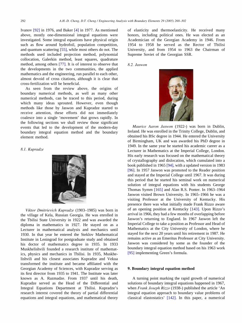
A.H.-D. Cheng, D.T. Cheng / Engineering Analysis with Boundary Elements 29 (2005) 268–302292

Ivanov [92] in 1976, and Baker [4] in 1977. As mentioned

above, mostly one-dimensional integral equations were

investigated. Some integral equations have physical origin

such as flow around hydrofoil, population competition,

and quantum scattering [55], while most others do not. The

methods used included projection method, polynomial

collocation, Galerkin method, least squares, quadrature

method, among others [77]. It is of interest to observe that

the developments in the two communities, the applied

mathematics and the engineering, run parallel to each other,

almost devoid of cross citations, although it is clear that

cross-fertilization will be beneficial.

As seen from the review above, the origins of

boundary numerical methods, as well as many other

numerical methods, can be traced to this period, during

which many ideas sprouted. However, even though

methods like those by Jaswon and Kupradze started to

receive attention, these efforts did not immediately

coalesce into a single ‘movement’ that grows rapidly. In

the following sections we shall review those significant

events that led to the development of the modern-day

boundary integral equation method and the boundary

element method.

8.1. Kupradze

Viktor Dmitrievich Kupradze (1903–1985) was born in

the village of Kela, Russian Georgia. He was enrolled in

the Tbilisi State University in 1922 and was awarded the

diploma in mathematics in 1927. He stayed on as a

Lecturer in mathematical analysis and mechanics until

1930. In that year he entered the Steklov Mathematical

Institute in Leningrad for postgraduate study and obtained

his doctor of mathematics degree in 1935. In 1933

Muskhelishvili founded a research institute of mathemat-

ics, physics and mechanics in Tbilisi. In 1935, Muskhe-

lishvili and his closest associates Kupradze and Vekua

transformed the institute and became affiliated with the

Georgian Academy of Sciences, with Kupradze serving as

its first director from 1935 to 1941. The Institute was later

known as A. Razmadze. From 1937 until his death,

Kupradze served as the Head of the Differential and

Integral Equations Department at Tbilisi. Kupradze’s

research interest covered the theory of partial differential

equations and integral equations, and mathematical theory

of elasticity and thermoelasticity. He received many

honors, including political ones. He was elected as an

Academician of the Georgian Academy in 1946. From

1954 to 1958 he served as the Rector of Tbilisi

University, and from 1954 to 1963 the Chairman of

Supreme Soviet of the Georgian SSR.

8.2. Jaswon

Maurice Aaron Jaswon (1922-) was born in Dublin,

Ireland. He was enrolled in the Trinity College, Dublin, and

obtained his BSc degree in 1944. He entered the University

of Birmingham, UK and was awarded his PhD degree in

1949. In the same year he started his academic career as a

Lecturer in Mathematics at the Imperial College, London.

His early research was focused on the mathematical theory

of crystallography and dislocation, which cumulated into a

book published in 1965 [94], with a updated version in 1983

[96]. In 1957 Jaswon was promoted to the Reader position

and stayed at the Imperial College until 1967. It was during

this period that he started his seminal work on numerical

solution of integral equations with his students George

Thomas Symm [165] and Alan R.S. Ponter. In 1963–1964

Jaswon visited Brown University. In 1965–1966 he was a

visiting Professor at the University of Kentucky. His

presence there was what initially made Frank Rizzo aware

of an opening position at Kentucky [143]. Upon Rizzo’s

arrival in 1966, they had a few months of overlapping before

Jaswon’s returning to England. In 1967 Jaswon left the

Imperial College to take a position as Professor and Head of

Mathematics at the City University of London, where he

stayed for the next 20 years until his retirement in 1987. He

remains active as an Emeritus Professor at City University.

Jaswon was considered by some as the founder of the

boundary integral equation method based on his 1963 work

[95] implementing Green’s formula.

9. Boundary integral equation method

A turning point marking the rapid growth of numerical

solutions of boundary integral equations happened in 1967,

when Frank Joseph Rizzo (1938-) published the article ‘An

integral equation approach to boundary value problems of

classical elastostatics’ [142]. In this paper, a numerical

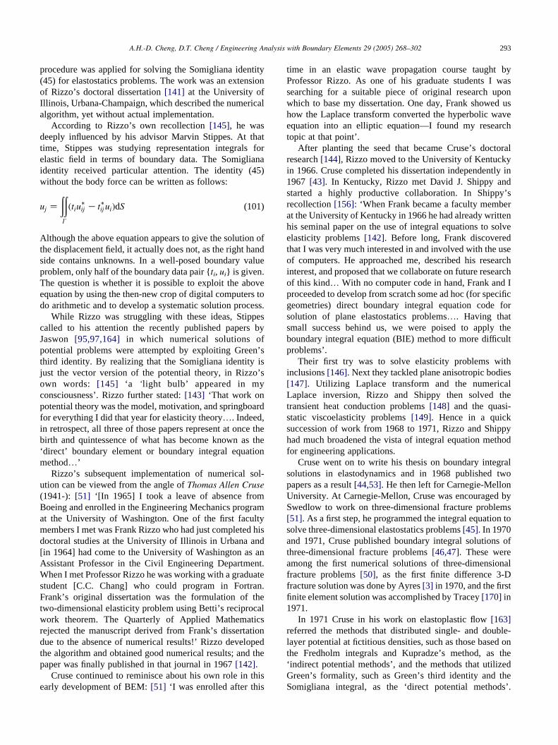
A.H.-D. Cheng, D.T. Cheng / Engineering Analysis with Boundary Elements 29 (2005) 268–302 293

procedure was applied for solving the Somigliana identity

(45) for elastostatics problems. The work was an extension

of Rizzo’s doctoral dissertation [141] at the University of

Illinois, Urbana-Champaign, which described the numerical

algorithm, yet without actual implementation.

According to Rizzo’s own recollection [145], he was

deeply influenced by his advisor Marvin Stippes. At that

time, Stippes was studying representation integrals for

elastic field in terms of boundary data. The Somigliana

identity received particular attention. The identity (45)

without the body force can be written as follows:

uj Z

ððG

ðtiu�ij K t�ij uiÞdS (101)

Although the above equation appears to give the solution of

the displacement field, it actually does not, as the right hand

side contains unknowns. In a well-posed boundary value

problem, only half of the boundary data pair {ti, ui} is given.

The question is whether it is possible to exploit the above

equation by using the then-new crop of digital computers to

do arithmetic and to develop a systematic solution process.

While Rizzo was struggling with these ideas, Stippes

called to his attention the recently published papers by

Jaswon [95,97,164] in which numerical solutions of

potential problems were attempted by exploiting Green’s

third identity. By realizing that the Somigliana identity is

just the vector version of the potential theory, in Rizzo’s

own words: [145] ‘a ‘light bulb’ appeared in my

consciousness’. Rizzo further stated: [143] ‘That work on

potential theory was the model, motivation, and springboard

for everything I did that year for elasticity theory.. Indeed,

in retrospect, all three of those papers represent at once the

birth and quintessence of what has become known as the

‘direct’ boundary element or boundary integral equation

method.’

Rizzo’s subsequent implementation of numerical sol-

ution can be viewed from the angle of Thomas Allen Cruse

(1941-): [51] ‘[In 1965] I took a leave of absence from

Boeing and enrolled in the Engineering Mechanics program

at the University of Washington. One of the first faculty

members I met was Frank Rizzo who had just completed his

doctoral studies at the University of Illinois in Urbana and

[in 1964] had come to the University of Washington as an

Assistant Professor in the Civil Engineering Department.

When I met Professor Rizzo he was working with a graduate

student [C.C. Chang] who could program in Fortran.

Frank’s original dissertation was the formulation of the

two-dimensional elasticity problem using Betti’s reciprocal

work theorem. The Quarterly of Applied Mathematics

rejected the manuscript derived from Frank’s dissertation

due to the absence of numerical results!’ Rizzo developed

the algorithm and obtained good numerical results; and the

paper was finally published in that journal in 1967 [142].

Cruse continued to reminisce about his own role in this

early development of BEM: [51] ‘I was enrolled after this

time in an elastic wave propagation course taught by

Professor Rizzo. As one of his graduate students I was

searching for a suitable piece of original research upon

which to base my dissertation. One day, Frank showed us

how the Laplace transform converted the hyperbolic wave

equation into an elliptic equation—I found my research

topic at that point’.

After planting the seed that became Cruse’s doctoral

research [144], Rizzo moved to the University of Kentucky

in 1966. Cruse completed his dissertation independently in

1967 [43]. In Kentucky, Rizzo met David J. Shippy and

started a highly productive collaboration. In Shippy’s

recollection [156]: ‘When Frank became a faculty member

at the University of Kentucky in 1966 he had already written

his seminal paper on the use of integral equations to solve

elasticity problems [142]. Before long, Frank discovered

that I was very much interested in and involved with the use

of computers. He approached me, described his research

interest, and proposed that we collaborate on future research

of this kind. With no computer code in hand, Frank and I

proceeded to develop from scratch some ad hoc (for specific

geometries) direct boundary integral equation code for

solution of plane elastostatics problems.. Having that

small success behind us, we were poised to apply the

boundary integral equation (BIE) method to more difficult

problems’.

Their first try was to solve elasticity problems with

inclusions [146]. Next they tackled plane anisotropic bodies

[147]. Utilizing Laplace transform and the numerical

Laplace inversion, Rizzo and Shippy then solved the

transient heat conduction problems [148] and the quasi-

static viscoelasticity problems [149]. Hence in a quick

succession of work from 1968 to 1971, Rizzo and Shippy

had much broadened the vista of integral equation method

for engineering applications.

Cruse went on to write his thesis on boundary integral

solutions in elastodynamics and in 1968 published two

papers as a result [44,53]. He then left for Carnegie-Mellon

University. At Carnegie-Mellon, Cruse was encouraged by

Swedlow to work on three-dimensional fracture problems

[51]. As a first step, he programmed the integral equation to

solve three-dimensional elastostatics problems [45]. In 1970

and 1971, Cruse published boundary integral solutions of

three-dimensional fracture problems [46,47]. These were

among the first numerical solutions of three-dimensional

fracture problems [50], as the first finite difference 3-D

fracture solution was done by Ayres [3] in 1970, and the first

finite element solution was accomplished by Tracey [170] in

1971.

In 1971 Cruse in his work on elastoplastic flow [163]

referred the methods that distributed single- and double-

layer potential at fictitious densities, such as those based on

the Fredholm integrals and Kupradze’s method, as the

‘indirect potential methods’, and the methods that utilized

Green’s formality, such as Green’s third identity and the

Somigliana integral, as the ‘direct potential methods’.

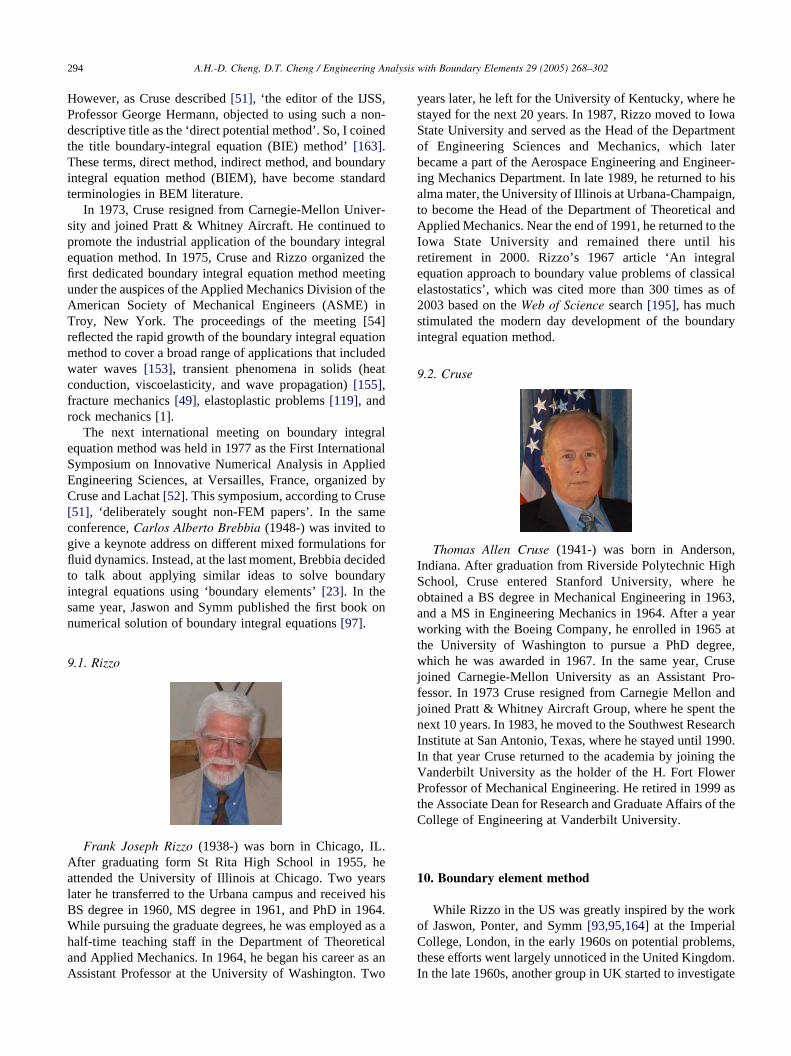
A.H.-D. Cheng, D.T. Cheng / Engineering Analysis with Boundary Elements 29 (2005) 268–302294

However, as Cruse described [51], ‘the editor of the IJSS,

Professor George Hermann, objected to using such a non-

descriptive title as the ‘direct potential method’. So, I coined

the title boundary-integral equation (BIE) method’ [163].

These terms, direct method, indirect method, and boundary

integral equation method (BIEM), have become standard

terminologies in BEM literature.

In 1973, Cruse resigned from Carnegie-Mellon Univer-

sity and joined Pratt & Whitney Aircraft. He continued to

promote the industrial application of the boundary integral

equation method. In 1975, Cruse and Rizzo organized the

first dedicated boundary integral equation method meeting

under the auspices of the Applied Mechanics Division of the

American Society of Mechanical Engineers (ASME) in

Troy, New York. The proceedings of the meeting [54]

reflected the rapid growth of the boundary integral equation

method to cover a broad range of applications that included

water waves [153], transient phenomena in solids (heat

conduction, viscoelasticity, and wave propagation) [155],

fracture mechanics [49], elastoplastic problems [119], and

rock mechanics [1].

The next international meeting on boundary integral

equation method was held in 1977 as the First International

Symposium on Innovative Numerical Analysis in Applied

Engineering Sciences, at Versailles, France, organized by

Cruse and Lachat [52]. This symposium, according to Cruse

[51], ‘deliberately sought non-FEM papers’. In the same

conference, Carlos Alberto Brebbia (1948-) was invited to

give a keynote address on different mixed formulations for

fluid dynamics. Instead, at the last moment, Brebbia decided

to talk about applying similar ideas to solve boundary

integral equations using ‘boundary elements’ [23]. In the

same year, Jaswon and Symm published the first book on

numerical solution of boundary integral equations [97].

9.1. Rizzo

Frank Joseph Rizzo (1938-) was born in Chicago, IL.

After graduating form St Rita High School in 1955, he

attended the University of Illinois at Chicago. Two years

later he transferred to the Urbana campus and received his

BS degree in 1960, MS degree in 1961, and PhD in 1964.

While pursuing the graduate degrees, he was employed as a

half-time teaching staff in the Department of Theoretical

and Applied Mechanics. In 1964, he began his career as an

Assistant Professor at the University of Washington. Two

years later, he left for the University of Kentucky, where he

stayed for the next 20 years. In 1987, Rizzo moved to Iowa

State University and served as the Head of the Department

of Engineering Sciences and Mechanics, which later

became a part of the Aerospace Engineering and Engineer-

ing Mechanics Department. In late 1989, he returned to his

alma mater, the University of Illinois at Urbana-Champaign,

to become the Head of the Department of Theoretical and

Applied Mechanics. Near the end of 1991, he returned to the

Iowa State University and remained there until his

retirement in 2000. Rizzo’s 1967 article ‘An integral

equation approach to boundary value problems of classical

elastostatics’, which was cited more than 300 times as of

2003 based on the Web of Science search [195], has much

stimulated the modern day development of the boundary

integral equation method.

9.2. Cruse

Thomas Allen Cruse (1941-) was born in Anderson,

Indiana. After graduation from Riverside Polytechnic High

School, Cruse entered Stanford University, where he

obtained a BS degree in Mechanical Engineering in 1963,

and a MS in Engineering Mechanics in 1964. After a year

working with the Boeing Company, he enrolled in 1965 at

the University of Washington to pursue a PhD degree,

which he was awarded in 1967. In the same year, Cruse

joined Carnegie-Mellon University as an Assistant Pro-

fessor. In 1973 Cruse resigned from Carnegie Mellon and

joined Pratt & Whitney Aircraft Group, where he spent the

next 10 years. In 1983, he moved to the Southwest Research

Institute at San Antonio, Texas, where he stayed until 1990.

In that year Cruse returned to the academia by joining the

Vanderbilt University as the holder of the H. Fort Flower

Professor of Mechanical Engineering. He retired in 1999 as

the Associate Dean for Research and Graduate Affairs of the

College of Engineering at Vanderbilt University.

10. Boundary element method

While Rizzo in the US was greatly inspired by the work

of Jaswon, Ponter, and Symm [93,95,164] at the Imperial

College, London, in the early 1960s on potential problems,

these efforts went largely unnoticed in the United Kingdom.

In the late 1960s, another group in UK started to investigate

A.H.-D. Cheng, D.T. Cheng / Engineering Analysis with Boundary Elements 29 (2005) 268–302 295

integral equations. According to Watson [191]: ‘I was

introduced to boundary integral equations in 1966, as a

research student at the University of Southampton under

Hugh Tottenham. Tottenham possessed a remarkable

library of Soviet books, and encouraged research students to

explore possible applications of the work of Muskhelishvili

[126], Kupradze [104] and others. I laboured through

Muskhelishvili’s complex variable theory, and struggled

with Kupradze’s tortuous mathematical notation without the

benefit of being able to read the text.. I pondered among

other things the problems posed by edges and corners and

came to understand that the fictitious force densities would

probably tend to infinity near such features. My attempts to

determine the nature of the supposed singularities, however,

were unsuccessful.’ Doctoral dissertations based on indirect

methods of Kupradze produced around this time included

that by Banerjee [6] in 1970, and Watson [190] and Tomlin

[169] in 1973.

At that time, Brebbia was also a PhD student at the

University of Southampton under Tottenham. His research

was on the numerical solution of complex double curved

shell structures and he investigated a range of techniques

including variational methods, finite elements, and integral

equations [18]. As a part of his dissertation work, Brebbia

spent 18 months at Massachusetts Institute of Technology,

first working with Eric Reissner (1913–1996), and then

Jerry Connor. Reissner’s introduction of the mixed

formulations of variational principles coupled with Breb-

bia’s knowledge of integral equations gave Brebbia a better

understanding of the generalized weak formulations. Jerry

Connor was at that time carrying out research in the solution

of mixed formulations using finite elements. The collabor-

ation between Brebbia and Connor resulted in two finite

element books [24, 39].

With his new knowledge, Brebbia returned to South-

ampton and completed his thesis on shell analysis [18]. He

was appointed a Lecturer at the Civil Engineering Depart-

ment. He continued his effort in producing integral equation

result for complex shell elements, but decided it was

insufficiently versatile to warrant further development. It

was in 1970 that Brebbia gave his PhD student Jean-Claude

Lachat the task of developing boundary integral equation

formulation seeking to obtain the same versatility as curved

finite elements.

Until that time, the US and the UK schools have been

largely working in isolation from each other, except for the

influence of Jaswon’s work on Rizzo’s research, and the

fundamental ideas of mixed formulations migrated from

MIT to Southampton by Brebbia. In 1972, Brebbia was

organizing the First International Conference on Variational

Methods in Engineering at Southampton with Tottenham

[27]. Although both organizers were working on integral

equations at that time, the inclusion of a special session on

this subject was an afterthought on the assumption that it

would be possible to tie the boundary integral equations

with the variational formulation. Brebbia invited Cruse to

deliver an opening lecture on the boundary-integral

equation method in the conference [48]. As recalled by

Brebbia [22]: ‘Since the beginning of the 1960s, a group

existed at Southampton University working on applications

of integral equations in engineering. Our work was up to

then directly related to the European Mathematical Schools

that originated in Russia. The inclusion of Boundary

Integral Equations as one of the topics of the conference

was a last moment decision, as up to then they were not

interpreted in a variational way. Meeting Tom opened to

us the scenario of the research in BIE taking place in

America, most of it related to his work. It was a historical

landmark for our group and from then on, we continued to

collaborate very closely with Tom’.

The above conference was also the occasion for Brebbia,

Cruse, and Lachat to get together to discuss the latest

research. Lachat went on to offer Watson a position in his

laboratory through Brebbia [23]. In Watson’s recollection

[191]: ‘Towards the end of 1971 I was contacted by

Brebbia, who asked that I pay him an overnight visit to

discuss the implementation of boundary element methods

with his external PhD student, Jean-Claude Lachat. .Lachat discussed with me through Brebbia as interpreter

some aspects of boundary elements, and then produced a job

application form, requesting that I reply to his offer within

four weeks. . I decided to accept. Lachat, . was head of

the Departement Theorique et Engrenages [at Centre

Technique des Industries Mecaniques] . At the beginning

of 1973 I started work on boundary elements. I was to

develop firstly a program for plane strain, then one for three

dimensional analysis. Lachat knew of the work of Rizzo and

Cruse, and proposed that the direct formulation be used. I

readily agreed, having met Cruse in 1972 and discussed with

him the direct and indirect approaches. The finite element

programming had been most instructive in respect of shape

functions, Gaussian quadrature and out-of-core simul-

taneous equation solution techniques. It seemed clear that

the boundary elements should be isoparametric, with at least

quadratic variation so that curved surfaces could be

modelled accurately. Analytical integration was then out

of the question, and Gaussian quadrature was far superior to

Simpson’s rule. Adaptations of Gaussian quadrature could

integrate weakly singular functions, but Cauchy principal

values could not be computed directly by quadrature. . The

problem of Cauchy principal values was solved by not

calculating them’. Lachat finished his dissertation in 1975

[107], and the paper of Lachat and Watson [108] was

published in 1976, which was considered as the first

published work that incorporates the above-mentioned finite

element ideas into boundary integral method.

Up to 1977 the numerical method for solving integral

equations had been called the ‘boundary integral equation

method’, following Cruse’s naming. However, with the

growing popularity of the finite element method, it became

clear that many of the finite element ideas can be applied to

the numerical technique solving boundary integral

A.H.-D. Cheng, D.T. Cheng / Engineering Analysis with Boundary Elements 29 (2005) 268–302296

equations. This is particularly demonstrated in the work of

Lachat and Watson [108]. Furthermore, parallel to the

theoretical development of finite element method, it was

shown that the weighted residual technique can be used to

derive the boundary integral equations [19,25]. The term

‘boundary element method,’ mirroring ‘finite element

method,’ finally emerged in 1977.

The creation of the term ‘boundary element method’ was

a collective effort by the research group at the University of

Southampton. According to Jose Dominguez [57]: ‘The

term Boundary Element Method was coined by C.A.

Brebbia, J. Dominguez, P. K. Banerjee and R. Butterfield

at the University of Southampton. It was used for the first

time in three publications of these authors appeared in 1977:

a journal paper by Brebbia and Dominguez [25], a [chapter

in book] by Banerjee and Butterfield [7], and Dominguez’s

PhD Thesis [56] (in Spanish). Those four authors never

wrote a paper on the subject together but they collectively

came to this name at the University of Southampton. At that

time, R. Butterfield was a [Senior Lecturer], C.A. Brebbia

was a Senior Lecturer, J. Dominguez was a Visiting

Research Fellow, and P.K. Banerjee, who had been student

and researcher at Southampton [earlier], was a frequent

visitor. In some occasions, this group or part of it, met for

lunch at the University or even participated at courses

organized by Carlos Brebbia in Southampton or London.

The phrase Boundary Element Method came out as part of

the discussions in one of these meetings and was used by all

of them in their immediate work.’ (text in square brackets is

correction by the authors.) It was also stated in a preface by

Brebbia [19]: ‘The term ‘boundary element’ originated

within the Department of Civil Engineering at Southampton

University. It is used to indicate the method whereby the

external surface of a domain is divided into a series of

elements over which the functions under consideration can

vary in different ways, in much the same manner as in finite

elements.’

Brebbia presented the boundary element method using

the weighted residuals formulation [19,21,25]. The devel-

opment of solving boundary value problems using functions

defined on local domains with low degree of continuity was

strongly influenced by the development of extended

variational principles and weighted residuals in the mid

1960s. Key players included Eric Reissner [139] and

Kyuichiro Washizu [187], who pioneered the use of

mixed variational statements that allowed the flexibility in

choosing localized functions. To deal with non-conservative

and time-dependent problems, the strategy shifted from the

variational approach to the method of weighted residuals

combined with the concept of weak forms. Brebbia [19]

showed that one could generate a spectrum of methods

ranging from finite elements to boundary elements.

Consider a function f satisfying the linear partial

differential operator L in the following fashion

Lffg Z bðxÞ; x2U (102)

and subject to the essential and natural boundary conditions

Sffg Z f ðxÞ; x2G1

Nffg Z gðxÞ; x2G2

(103)

where S and N are the corresponding differential operators.

Our goal is to find the approximate solution that minimizes

the error with respect to a weighing function w in

the following fashion:

hLffgKb;wiU

Z hNffgKg; S�fwgiG2K hSffgK f ;N�fwgiG1

(104)

where S* and N* are the adjoint operators of S and N, and the

angle brackets denote the inner product,

ha;big Z

ðg

aðxÞbðxÞdx (105)

Eq. (104) can be considered as the theoretical basis for a

number of numerical methods [19]. For example, finite

difference can be interpreted as a method using Dirac delta

function as the weighing function and enforcing the boundary

conditions exactly. The well-known Galerkin formulation in

finite element method uses of the basis function for w the same

as that used for the approximation of f.

For the boundary element formulation, we perform

integration by parts on (104) for as many times as necessary

to obtain

hf;L�fwgiU Z hSffg;N�fwgiG2K hNffg; S�fwgiG1

C hf ;N�fwgiG1K hg; S�fwgiG2

C hb;wiU

(106)

where L� is the adjoint operators of L. The idea for the

boundary method is to replace w by the fundamental

solution G*, which satisfies

L�fG�g Z d (107)

such that (106) reduces to

f Z hSffg;N�fG�giG2K hNffg; S�fG�giG1

C hf ;N�fG�giG1K hg; S�fG�giG2

C hb;G�iU (108)

This is the weighted residual formulation for boundary

element method. For the case of Laplace equation, which is

self-adjoint, with the boundary conditions

f Z f ðxÞ; x2G1

vf

vnZ gðxÞ; x2G2

(109)

A.H.-D. Cheng, D.T. Cheng / Engineering Analysis with Boundary Elements 29 (2005) 268–302 297

Eq. (108) becomes

f ZK1

4p

ððG1

1

r

vf

vndS C

1

4p

ððG1

fvð1=rÞ

vndS

K1

4p

ððG2

1

rg dS C

1

4p

ððG2

fvð1=rÞ

vndS (110)

which is just Green’s formula (25) with boundary conditions

substituted in.

In commissioning the term ‘boundary element method’,

Brebbia considered that the method would gain in generality

if it was based on the mixed principles and weighted

residual formulations. Others have used different interpret-

ations. For example, Banerjee and Butterfield [7] in 1977

followed Kupradze’s idea of distributing sources for solving

potential problems and forces for elasticity problems, and

also called it ‘boundary element method.’ Similarly, the

articles by Brady and Bray [16,17] in 1978 used the term

BEM, but were also based on the indirect formulation. Even

in Brebbia’s 1978 book on boundary element method [19],

the indirect formulation was considered, thought not in

details.

In the subsequent years, the term BEM has been broadly

used as a generic term for a number of boundary based

numerical schemes, whether ‘elements’ were used or not.

The present article will not argue whether in certain

instances the term boundary element is a misnomer or not.

As the present review has demonstrated, the theoretical

foundations of these methods are closely related and the

histories of their development intertwined. Hence, as

indicated in Section 1, the present review accommodates

the broadest usage.

In 1978, Brebbia published the first textbook on BEM

‘The Boundary Element Method for Engineers’ [19]. The

book contained a series of computer codes developed by

Dominguez. In the same year, Brebbia organized the first

conference dedicated to the BEM: the First International

Conference on Boundary Element Methods, at the

University of Southampton [20]. This conference series

has become an annual event and is nowadays organized

by the Wessex Institute of Technology. The most recent

in the series as of this writing is the 26th conference in

2004 [26]. In 1984 Brebbia founded the Journal

‘Engineering Analysis—Innovations in Computational

Techniques.’ It initially published papers involving

boundary element as well as other numerical methods.

In 1989, the journal was renamed to ‘Engineering

Analysis with Boundary Elements’ and became a journal

dedicated to the boundary element method. The journal is

at the present published by Elsevier and enjoys a high

impact factor among the engineering science and

numerical method journals.

10.1. Brebbia

Carlos Alberto Brebbia (1938-) was born in Rosario,

Argentina. He received a BS degree in civil engineering

from the University of Litoral, Rosario. He did early

research on the application of Volterra equations to creep

buckling and other problems. His mentor there was Jose

Nestor Distefano, latterly of the University of California,

Berkeley. Brebbia went to the University of Southampton,

UK to carry out his PhD study under Hugh Tottenham.

During the whole 1966 and first 6 months in 1967, he

visited MIT and conducted research under Eric Reissner

and Jerry Connor. He attributed his success with FEM as

well as BEM to these great teachers. Brebbia was granted

his PhD at Southampton in 1967. After a year’s research

at the UK Electricity Board Laboratories, in 1970 Brebbia

started working as a Lecturer at Southampton. In 1975, he

accepted a position as Associate Professor at Princeton

University, where he stayed for over a year. He then

returned to Southampton where he eventually became a

Reader. In 1979, Brebbia was again in the US holding a

full professor position at the University of California,

Irvine. In 1981, he moved back to the UK and founded

the Wessex Institute of Technology as an international

focus for BEM research. He has been serving as its

Director since.

11. Conclusion

In this article we reviewed the heritage and the early

history of the boundary element method The heritage is

traced to its mathematical foundation developed in the late

eighteenth to early 18th century, in terms of the Laplace

equation, the existence and uniqueness of solution of

boundary value problems, the Gauss and Stokes theorems

that allowed the reduction in spatial dimensions, the Green’s

identities, Green’s function, the Fredholm integral

equations, and the extension of Green’s formula to

acoustics, elasticity, and other physical problems. The

pioneers behind these mathematical developments were

celebrated with short biographies.

We then observe that in the first half of the 20th century

there existed various attempts to find numerical solutions

without the aid of the modern day electronic computers.

Once electronic computers became widely available, 1960s

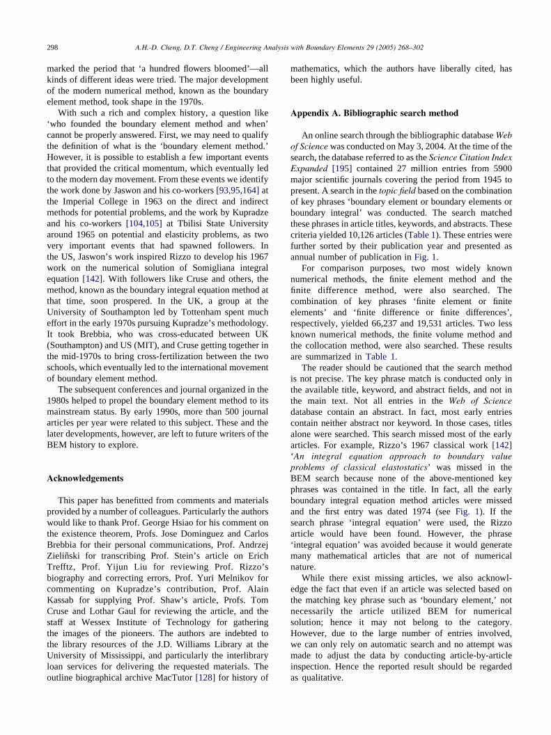
A.H.-D. Cheng, D.T. Cheng / Engineering Analysis with Boundary Elements 29 (2005) 268–302298

marked the period that ‘a hundred flowers bloomed’—all

kinds of different ideas were tried. The major development

of the modern numerical method, known as the boundary

element method, took shape in the 1970s.

With such a rich and complex history, a question like

‘who founded the boundary element method and when’

cannot be properly answered. First, we may need to qualify

the definition of what is the ‘boundary element method.’

However, it is possible to establish a few important events

that provided the critical momentum, which eventually led

to the modern day movement. From these events we identify

the work done by Jaswon and his co-workers [93,95,164] at

the Imperial College in 1963 on the direct and indirect

methods for potential problems, and the work by Kupradze

and his co-workers [104,105] at Tbilisi State University

around 1965 on potential and elasticity problems, as two

very important events that had spawned followers. In

the US, Jaswon’s work inspired Rizzo to develop his 1967

work on the numerical solution of Somigliana integral

equation [142]. With followers like Cruse and others, the

method, known as the boundary integral equation method at

that time, soon prospered. In the UK, a group at the

University of Southampton led by Tottenham spent much

effort in the early 1970s pursuing Kupradze’s methodology.

It took Brebbia, who was cross-educated between UK

(Southampton) and US (MIT), and Cruse getting together in

the mid-1970s to bring cross-fertilization between the two

schools, which eventually led to the international movement

of boundary element method.

The subsequent conferences and journal organized in the

1980s helped to propel the boundary element method to its

mainstream status. By early 1990s, more than 500 journal

articles per year were related to this subject. These and the

later developments, however, are left to future writers of the

BEM history to explore.

Acknowledgements

This paper has benefitted from comments and materials

provided by a number of colleagues. Particularly the authors

would like to thank Prof. George Hsiao for his comment on

the existence theorem, Profs. Jose Dominguez and Carlos

Brebbia for their personal communications, Prof. Andrzej

Zielinski for transcribing Prof. Stein’s article on Erich

Trefftz, Prof. Yijun Liu for reviewing Prof. Rizzo’s

biography and correcting errors, Prof. Yuri Melnikov for

commenting on Kupradze’s contribution, Prof. Alain

Kassab for supplying Prof. Shaw’s article, Profs. Tom

Cruse and Lothar Gaul for reviewing the article, and the

staff at Wessex Institute of Technology for gathering

the images of the pioneers. The authors are indebted to

the library resources of the J.D. Williams Library at the

University of Mississippi, and particularly the interlibrary

loan services for delivering the requested materials. The

outline biographical archive MacTutor [128] for history of

mathematics, which the authors have liberally cited, has

been highly useful.

Appendix A. Bibliographic search method

An online search through the bibliographic database Web

of Science was conducted on May 3, 2004. At the time of the

search, the database referred to as the Science Citation Index

Expanded [195] contained 27 million entries from 5900

major scientific journals covering the period from 1945 to

present. A search in the topic field based on the combination

of key phrases ‘boundary element or boundary elements or

boundary integral’ was conducted. The search matched

these phrases in article titles, keywords, and abstracts. These

criteria yielded 10,126 articles (Table 1). These entries were

further sorted by their publication year and presented as

annual number of publication in Fig. 1.

For comparison purposes, two most widely known

numerical methods, the finite element method and the

finite difference method, were also searched. The

combination of key phrases ‘finite element or finite

elements’ and ‘finite difference or finite differences’,

respectively, yielded 66,237 and 19,531 articles. Two less

known numerical methods, the finite volume method and

the collocation method, were also searched. These results

are summarized in Table 1.

The reader should be cautioned that the search method

is not precise. The key phrase match is conducted only in

the available title, keyword, and abstract fields, and not in

the main text. Not all entries in the Web of Science

database contain an abstract. In fact, most early entries

contain neither abstract nor keyword. In those cases, titles

alone were searched. This search missed most of the early

articles. For example, Rizzo’s 1967 classical work [142]

‘An integral equation approach to boundary value

problems of classical elastostatics’ was missed in the

BEM search because none of the above-mentioned key

phrases was contained in the title. In fact, all the early

boundary integral equation method articles were missed

and the first entry was dated 1974 (see Fig. 1). If the

search phrase ‘integral equation’ were used, the Rizzo

article would have been found. However, the phrase

‘integral equation’ was avoided because it would generate

many mathematical articles that are not of numerical

nature.

While there exist missing articles, we also acknowl-

edge the fact that even if an article was selected based on

the matching key phrase such as ‘boundary element,’ not

necessarily the article utilized BEM for numerical

solution; hence it may not belong to the category.

However, due to the large number of entries involved,

we can only rely on automatic search and no attempt was

made to adjust the data by conducting article-by-article

inspection. Hence the reported result should be regarded

as qualitative.

A.H.-D. Cheng, D.T. Cheng / Engineering Analysis with Boundary Elements 29 (2005) 268–302 299

References

[1] Altiero NJ, Sikarskie DL. An integral equation method applied to

penetration problems in rock mechanics. In: Cruse TA, Rizzo FJ,

editors. Boundary-integral equation method: computational appli-

cations in applied mechanics, AMD-vol. 11, 1975. p. 119–41.

[2] Atkinson KE. A survey of numerical methods for the solution of

fredholm integral equations of the second kind. SIAM 1976.

[3] Ayres DJ. A numerical procedure for calculating stress and

deformation near a slit in a three dimensional elastic plastic solid.

Eng Fract Mech 1970;2:87–106.

[4] Baker CTH. The numerical treatment of integral equations. Oxford:

Oxford University Press; 1977.

[5] Banaugh RP, Goldsmith W. Diffraction of steady acoustic waves by

surfaces of arbitrary shape. J Acoust Soc Am 1963;35:1590–601.

[6] Banerjee PK. A contribution to the study of axially loaded pile

foundations. PhD Thesis. University of Southampton; 1970.

[7] Banerjee PK, Butterfield R. Boundary element method in geome-

chanics. In: Gudehus G, editor. Finite elements in geomechanics.

New York: Wiley; 1977. p. 529–70. Chapter 16.

[8] Belhoste B. Augustin-Louis Cauchy. A biography. Berlin: Springer;

1991.

[9] Belytschko T, Lu YY, Gu L. Element-free Galerkin methods. Int

J Numer Meth Engng 1994;37:229–56.

[10] Betti E. Teoria della elasticita. Nuovo Cimento, Ser 1872;2:6–10.

[11] Betti E. Sopra l’equazioni di equilibrio dei corpi solidi elastici.

Annali delle Universita Toscane 1874;10:143–58.

[12] Bilby BA. Continuous distributions of dislocations. In: Sneddon IN,

Hill R, editors. Progress in solid mechanics. Amsterdam: North-

Holland; 1960. p. 329–98.

[13] Birkhoff GD. Oliver Dimon Kellogg—in memoriam. Bull Am Math

Soc 1933;39:171–7.

[14] Bogomolny A. Fundamental solutions method for elliptic boundary

value problems. SIAM J Numer Anal 1985;22:644–69.

[15] Boyer CB. A history of mathematics. 2nd ed. New York: Wiley;

1991.

[16] Brady BHG, Bray JW. Boundary element method for determining

stresses and displacements around long opening in a triaxial stress-

field. Int J Rock Mech Min Sci 1978;15:21–8.

[17] Brady BHG, Bray JW. Boundary element method for elastic analysis

of tabular orebody extraction, assuming complete plane strain. Int

J Rock Mech Min Sci 1978;15:29–37.

[18] Brebbia CA. On hyperbolic paraboloidal shells. PhD Thesis,

University of Southampton; 1968.

[19] Brebbia CA. The boundary element method for engineers.

London/New York: Pentech Press/Halstead Press; 1978.

[20] Brebbia CA, editor. Recent advances in boundary element methods.

Proceedings of first internatonal conference on boundary element

methods, University of Southampton.

[21] Brebbia CA. Introduction to boundary element methods. In:

Brebbia CA, editor. Recent advances in boundary element methods,

Proceedings of first international confeerence on boundary element

methods. Pentech: University of Southampton; 1978. p. 1–42.

[22] Brebbia CA. Tribute to Tom Cruse, Tom Cruse Commemorative

Issue. In: Brebbia CA, Cheng AH-D, editors. Eng Anal Bound Elem,

24, 2000. p. 701.

[23] Brebbia CA. personal communication; 2004.

[24] Brebbia CA, Connor JJ. Fundamentals of finite element techniques

for structural engineers. London: Butterworth; 1973.

[25] Brebbia CA, Dominguez J. Boundary element methods for potential

problems. Appl Math Modell 1977;1:372–8.

[26] Brebbia CA. Boundary elements XXVI. Proceedings of 26th

international conference on boundary element methods. Bologna,

Italy: WIT Press; 2004.

[27] Brebbia CA, Tottenham H. The first international conference on

variational methods in engineering. University of Southampton, UK

1972.

[28] Brunner H. 1896–1996: One hundred years of Volterra integral

equations of the first kind. Appl Numer Math 1997;24:83–93.

[29] Buckner HF. Die praktische Behandlung von Integralgleichungen.

Berlin: Springer; 1952.

[30] Buhler WK, Gauss A. Gauss, a biographical study. Berlin: Springer;

1981.

[31] Burton DM. The history of mathematics—an introduction. Newton,

MA: Allyn and Bacon; 1985.

[32] Cahan D, editor. Hermann von Helmholtz and the foundation of

nineteenth century science. Berkeley, CA: U. California Press;

1993.

[33] Cannell DM. George Green, mathematician and physicist 1793–

1841, the background to his life and work. 2nd ed.: SIAM; 2001.

[34] Cauchy A-L. Memoire sur les integrales definies, Memoires des

divers savants, ser 2 1;1827:601-799 [written 1814].

[35] Cauchy A-L. Lecons sur les applications de calcul infinitesimal a la

geometries; 1826–1828.

[36] Chen LH, Schweikert DG. Sound radiation from an arbitrary body.

J Acoust Soc Am 1963;35:1626–32.

[37] Chertock G. Sound radiation from vibrating surfaces. J Acoust Soc

Am 1964;36:1305–13.

[38] Clough RW. The finite element method in plane stress analysis.

Proceedings of second ASCE Conference on electronic computation;

1960.

[39] Connor JJ, Brebbia CA. Finite element techniques for fluid flow.

London: Newnes–Butterworths; 1976.

[40] Copley LG. Integral equation method for radiation from vibrating

bodies. J Acoust Soc Am 1967;41:807–16.

[41] Copley LG. Fundamental results concerning integral representation

in acoustic radiation. J Acoust Soc Am 1968;44:28–32.

[42] Costabel M. Boundary integral operators on Lipschitz domains:

elementary results. SIAM J Math Anal 1988;19:613–26.

[43] Cruse TA. The transient problem in classical elastodynamics solved

by integral equations. Doctoral dissertation. University of Washing-

ton; 1967, 117 pp.

[44] Cruse TA. A direct formulation and numerical solution of the general

transient elastodynamic problem—II. J Math Anal Appl 1968;22:

341–55.

[45] Cruse TA. Numerical solutions in three dimensional elastostatics. Int

J Solids Struct 1969;5:1259–74.

[46] Cruse TA. Lateral constraint in a cracked, three-dimensional elastic

body. Int J Fract Mech 1970;6:326–8.

[47] Cruse TA, VanBuren W. Three-dimensional elastic stress analysis of

a fracture specimen with an edge crack. Int J Fract Mech 1971;7:

1–15.

[48] Cruse TA. In: Brebbia CA, Tottenham H, editors. Application of the

boundary-integral equation solution method in solid mechanics.

Variational method in engineering, vol. II, Proceedings of an

international conference. Southampton: Southampton University

Press; 1972. p. 9–929.

[49] Cruse TA. Boundary-integral equation fracture mechanics analysis.

In: Cruse TA, Rizzo FJ, editors. Boundary-integral equation method:

computational applications in applied mechanics, AMD-vol. 11,

1975. p. 31–46.

[50] Cruse TA. BIE fracture mechanics: 25 years of developments. Comp

Mech 1996;18:1–11.

[51] Cruse TA. Boundary integral equations—a personal view. In:

Brebbia CA, Cheng AH-D, editors. Tom Cruse commemorative

issue: III. Eng Anal Bound Elem, 25, 2001. p. 709–12.

[52] Cruse TA, Lachat J-C. Proceedings of the international symposium

on innovative numerical analysis in applied engineering sciences,

Versailles, France; 1977.

[53] Cruse TA, Rizzo FJ. A direct formulation and numerical solution of

the general transient elastodynamic problem—I. J Math Anal Appl

1968;22:244–59.

A.H.-D. Cheng, D.T. Cheng / Engineering Analysis with Boundary Elements 29 (2005) 268–302300

[54] Cruse TA, Rizzo FJ. Boundary-integral equation method: compu-

tational applications in applied mechanics. Applied mechanics

conference, ASME, Rensselaer Polytechnic Institute, June 23–25,.

AMD-vol. 11 1975.

[55] Delves LM, Mohamed JL. Computational methods for integral

equations. Cambridge: Cambridge University Press; 1985.

[56] Dominguez J. Stress analysis around anchor plates: a boundary

element method application. PhD Thesis. Universidad de Sevilla;

1977.

[57] Dominguez J. personal communication; 2003.

[58] Dunham W. Euler, the master of us all. Math Assoc Am 1999.

[59] Ehrlich P. Kellogg, Bliss, Hedrick—Mizzou math pioneers.

Critical Points, 4. Department of Mathematics, University

of Missouri; 1999 [http://www.math.missouri.edu/wnews/issue4/

pioneers.html].

[60] Erdogan F, Gupta GD. Numerical solution of singular integral-

equations. Q J Appl Math 1972;29:525–34.

[61] Erdogan F, Gupta GD, Cook TS. Numerical solution of singular

integral equations. In: Sih GC, editor. Mechanics of fracture 1,

methods of analysis and solutions of crack problems, 1973. p. 368–

425.

[62] Eshelby JD. The continuum theory of lattice defects. Solid State

Phys 1956;3:79–114.

[63] Euler L. Principes generaux du mouvement des fluides. Mem Acad

Sci Berlin 1755;11:274–315.

[64] Euler L. Opera Omnia, Series prima: Opera mathematica (29

volumes), Series secunda: Opera mechanica et astronomica (31

volumes), Series tertia: Opera physica, Miscellanea (12 volumes),

Series quarta: A. Commercium epistolicum (10 volumes), edited by

the Euler Committee of the Swiss Academy of Science. Basel:

Birkhauser; 2003.

[65] Fairweather G, Karageorghis A. The method of fundamental

solutions for elliptic boundary value problems. Adv Comput Math

1998;9:69–95.

[66] Fourier JBJ. Theorie Analytique de la Chaleur (The analytical theory

of heat); 1822.

[67] Fredholm I. Sur une classe d’equations fonctionelles. Acta Math

1903;27:365–90.

[68] Friedman MB, Shaw R. Diffraction of pulse by cylindrical obstacles

of arbitrary cross section. J Appl Mech, Trans ASME 1962;29:40–6.

[69] Fritzius RS. In: Hsu JP, Zhang YZ, editors. Abbreviated biographical

sketch of Walter Ritz, Appendix. Lorentz and Poincare invariance—

100 years of realtivity. Singapore: World Scientific Publishers; 2003.

[70] Gauss CF. Theoria attractionis corporum sphaeroidicorum ellipti-

corum homogeneorum methodo novo tractata. Commentationes

societatis regiae scientiarum Gottingensis recentiores 1813;II:2–5.

[71] Gavelya SP. Periodical problems for shallow shells of arbitrary

curvature with apertures. Rep Ukrain Acad Sci 1969;8:703–8.

[72] Gegelia T, Jentsch L. Potential methods in continuum mechanics.

Georgian Math J 1994;1(6):599–640.

[73] Gellert W, Gottwald S, Hellwich M, Kastner H, Kustner H, editors.

The VNR concise encyclopedia of mathematics. 2nd ed. New York:

Van Nostrand Reinhold; 1989.

[74] Gerasoulis A. The use of piecewise quadratic polynomials for the

solution of singular integral equations of the Cauchy type. Comp

Math Appl 1982;8:15–22.

[75] Geroski PA. Models of technology diffusion. Res Policy 2000;29:

603–25.

[76] Gillispie CC. Pierre-Simon Laplace, 1749–1827, a life in exact

science. Princeton: Princeton University Press; 1997.

[77] Golberg MA. A survey of numerical methods for integral equations.

In: Golberg MA, editor. Solution methods for integral equations.

New York: Plenum Press; 1978. p. 1–58. Chapter 1.

[78] Gorgidze AY, Rukhadze AK. On the numerical solution of the

integral equations of the plane theory of elasticity. Soobshchenia

Gruz. Filiala A.N.S.S.S.R. 1940;1:255–8 [in Russian].

[79] Grabiner JV. The origin of Cauchy’s rigorous calculus. Cambridge,

MA: MIT Press; 1981.

[80] Grattan-Guinness I. Joseph Fourier, 1768–1830. Cambridge, MA:

MIT Press; 1972.

[81] Green G. An essay on the application of mathematical analysis to the

theories of electricity and magnetism. Printed for the Author by

Wheelhouse T. Nottigham; 1828. 72 p. Also, Mathematical papers of

George Green. Chelsea Publishing Co.; 1970. p. 1–115.

[82] Green G. In: Ferrers NM, editor. Mathematical papers of George

Green [reprinted by Chelsea Publ. Co., New York, 1970].

[83] Greenberg MD. Application of Green’s functions in science and

engineering. Englewood Cliffs, NJ: Prentice Hall; 1971.

[84] Gupta KK, Meek JL. A brief history of the beginning of the finite

element method. Int J Numer Meth Eng 1996;39:3761–74.

[85] Hadamard J. Theorie des equations aux derivees partielles lineaires

hyperboliques et du probleme de Cauchy. Acta Math 1908;31:

333–80.

[86] Hahn R. Laplace as a Newtonian Scientist, a paper delivered at a

Seminar on the Newtonian influence. Clark Library, UCLA; 1967.

[87] Helmholtz H. Theorie der Luftschwingungen in Rohren mit offenen

Enden. Journal fur die reine und angewandte Mathematik 1860;57:

1–72.

[88] Helmholtz H. Die Lehre von den Tonempfindungen, (On the

Sensations of Tone); 1863.

[89] Hess JL. Calculations of potential flow about bodies of revolution

having axes perpendicular to the free stream direction. J Aero Sci

1962;29:726–42.

[90] Hess JL. Review of integral-equation techniques for solving

potential-flow problems with emphasis on the surface source

method. Comp Meth Appl Mech Eng 1975;5:145–96.

[91] Hess JL, Smith AMO. Calculations of nonlifting potential flow about

arbitrary three-dimensional bodies. J Ship Res 1964;8:22–44.

[92] Ivanov VV. The theory of approximate methods and their application

to the numerical solution of singular integral equations.: Noordhoff;

1976 [Russian edition 1968].

[93] Jaswon MA. Integral equation methods in potential theory I. Proc R

Soc, A 1963;275:23–32.

[94] Jaswon MA. An introduction to mathematical crystallography. New

York: American Elsevier; 1965.

[95] Jaswon MA, Ponter AR. An integral equation solution of the torsion

problem. Proc R Soc, A 1963;273:237–46.

[96] Jaswon MA, Rose MA. Crystal symmetry: theory of colour

crystallography. New York: Halsted Press; 1983.

[97] Jaswon MA, Symm GT. Integral equation methods in potential

theory and elastostatics. London: Academic Press; 1977.

[98] Kagiwada H, Kalaba RE. Integral equations via imbedding methods.

New York: Addison-Wesley; 1974.

[99] Katz VJ. The history of Stokes theorem. Math Mag 1979;52:146–56.

[100] Kellogg OD. Foundations of potential theory.: Dover; 1953.

[101] Kelvin WT. Note on the integrations of the equations of equilibrium

of an elastic solid. Cambridge Dublin Math J 1848;3.

[102] Kolosov GV. On an application of complex function theory to a

plane problem of the mathematical theory of elasticity.: Yuriev;

1909 [in Russian].

[103] Kulakov VM, Tolkachev VM. Bending of plates of an arbitrary

shape. Rep Russ Acad Sci 1976;230.

[104] Kupradze VD. Potential methods in the theory of elasticity. In:

Sneddon IN, Hills R, editors. Israeli program for scientific

translation, 1965 [earlier edition: Kupradze VD, Dynamical

problems in elasticity, vol. III in Progress in solid mechanics, eds.

Sneddon IN, Hills R. North-Holland; 1963].

[105] Kupradze VD, Aleksidze MA. The method of functional equations

for the approximate solution of some boundary value problems. Zh

vichisl mat i mat fiz 1964;4:683–715 [in Russian].

[106] Kupradze VD, Gegelia TG, Basheleishvili MO, Burchuladze TV.

Three-dimensional problems of the mathematical theory of elasticity

and thermoelasticity.: North-Holland; 1979 [Russian edition 1976].

A.H.-D. Cheng, D.T. Cheng / Engineering Analysis with Boundary Elements 29 (2005) 268–302 301

[107] Lachat JC. A further development of the boundary integral technique

for elastostatics. Doctoral dissertation. University of Southampton;

1975.

[108] Lachat JC, Watson JO. Effective numerical treatment of boundary

integral equations: a formulation for three-dimensional elastostatics.

Int J Numer Meth Eng 1976;10:991–1005.

[109] Laplace PS. Histoire de l’Academie des Sciences de Paris, p. 135,

1782/85; p. 252, 1787/89.

[110] Lagrange J. Miscellanea Taurinasia 1760;2:273.

[111] Lagrange J-L. Memoires de l’Academie Royale des Sciences de

Paris. Savants etrangers 1773;VII.

[112] Lebesgue H. Sur des cas d’impossibilite du probleme de Dirichlet.

Comptes Rendus de la Societe Mathematique de France 1913;41:17.

[113] Lotz I. Calculation of potential flow past airship body in a yaw.

NACA TM 675 1932.

[114] Love AEH. A treatise on the mathematical theory of elasticity. 4th

ed. New York: Dover; 1944.

[115] Massonet CE. In: Zienkiewicz OC, Hollister GS, editors. Numerical

use of integral procedures. Stress analysis. New York: Wiley; 1965.

p. 198–235. Chapter 10.

[116] Mathon R, Johnston RL. The approximate solution of elliptic

boundary-value problems by fundamental solutions. SIAM J Numer

Anal 1977;14:638–50.

[117] Maxwell JC. On the calculation of the equilibrium and stiffness of

frames. Phil Mag 1864;27:294–9.

[118] Maz’ya V, Shaposhnikova T. Jacques Hadamard, a universal

mathematician. Am Math Soc 1998.

[119] Mendelson A, Albers LU. Application of boundary integral equation

to elastoplastic problems. In: Cruse TA, Rizzo FJ, editors. Boundary-

integral equation method: computational applications in applied

mechanics, AMD-vol. 11, 1975. p. 47–84.

[120] Mikhlin SG. Integral equations and their applications to certain

problems in mechanics, mathematical physics and technology. 2nd

rev ed. New York: Pergamon Press; 1964 [first Russian edition

1949].

[121] Mikhlin SG, Smolitsky JL. Approximation methods for the solution

of differential and integral equations. Amsterdam: Elsevier; 1967.

[122] Mitzner KM. Numerical solution for transient scattering from a hard

surface of arbitrary shape—retarded potential technique. J Acoust

Soc Am 1967;42:391–7.

[123] Morse PM, Feshbach H. Methods of theoretical physics. New York:

McGraw-Hill; 1953.

[124] Muskhelishvili NI. On the numerical solution of the plane problems

of the theory of elasticity. Trudy Tbilisskogo Matematicheskogo

Instituta 1937;1:83–7 [in Georgian].

[125] Muskhelishvili NI. Singular integral equations.: Noordhoff; 1953

[Russian edition 1946].

[126] Muskhelishvili NI. Some basic problems of the mathematical theory

of elasticity.: Noordhoof; 1959 [first Russian edition 1933].

[127] Oden JT. Historical comments on finite elements. In: Nash SG,

editor. A history of scientific computing. ACM Press; 1990. p. 152–

66.

[128] O’Connor JJ, Robertson EF. MacTutor history of mathematics

archive, [http://www-groups.dcs.st-and.ac.uk/history/; 2003.

[129] O’Donnell S. William Rowan Hamilton—portrait of a prodigy.

Dublin: Boole Press; 1983.

[130] Oliveira ERA. Plane stress analysis by a general integral method.

J Eng Mech Div, ASCE 1968;94:79–101.

[131] Peaceman DW. A personal retrospection of reservoir simulation. In:

Nash SG, editor. A history of scientific computing. ACM Press;

1990. p. 106–29.

[132] Poisson P-S. Bulletin de in soclete philomatique 1813;3:388.

[133] Ponter ARS. An integral equation solution of the inhomogeneous

torsion problem. J SIAM Appl Math 1966;14:819–30.

[134] Prager W. Die Druckverteilung an Korpern in ebener Potentialstro-

mung. Physik Zeitschr. 1928;29:865.

[135] Rankine WJM. On plane water-lines in two dimensions. Phil Trans

1864.

[136] Rayleigh JWS. Proc London Math Soc 1873;4:357–68.

[137] Rayleigh JWS.. 2nd ed The theory of sound. vols 1 and 2. New York:

Dover; 1945 [originally published in 1877].

[138] Rayleigh RJS. Life of John William Strutt, Third Baron Rayleigh

1924. London.

[139] Reissner E. On a variational theorem in elasticity. J Math Phys 1950;

29:90–5.

[140] Ritz W. Uber eine neue methode zur Losung gewissen variations—

Problems der mathematischen physik. J Reine Angew Math 1908;

135:1–61.

[141] Rizzo FJ. Some integral equation methods for plane problems of

classical elastostatics. Doctoral dissertation. University of Illinois,

Urbana-Champaign; 1964, p. 34.

[142] Rizzo FJ. An integral equation approach to boundary value problems

of classical elastostatics. Q Appl Math 1967;25:83–95.

[143] Rizzo FJ. The boundary element method, some early history—a

personal view. In: Beskos DE, editor. Boundary element methods in

structural analysis. ASCE; 1989. p. 1–16.

[144] Rizzo FJ. In honor of T.A. Cruse. In: Brebbia CA, Cheng AH-D,

editors. Tom Cruse Commemorative Issue. Eng Anal Bound Anal,

24, 2000. p. 703–5.

[145] Rizzo FJ. Springs, formulas and flatland: a path to boundary integral

methods in elasticity. Electron J Bound Elem 2003;1:1–7 [http://

tabula.rutgers.edu/EJBE/].

[146] Rizzo FJ, Shippy DJ. Formulation and solution procedure for the

general non-homogeneous elastic inclusion problem. Int J Solids

Struct 1968;4:1161–79.

[147] Rizzo FJ, Shippy DJ. A method for stress determination in plane

anisotropic bodies. J Compos Mater 1970;4:36–61.

[148] Rizzo FJ, Shippy DJ. A method of solution for certain problems of

transient heat conduction. AIAA J 1970;8:2004–9.

[149] Rizzo FJ, Shippy DJ. An application of the correspondence principle

of linear viscoelasticity theory. SIAM J Appl Math 1971;21:321–30.

[150] Schenck HA. Improved integral formulation for acoustic radiation

problems. J Acoust Soc Am 1968;44:41–58.

[151] Sharlin HI. Kelvin, William Thomson, Baron,. Encyclopædia

Britannica 2003.

[152] Shaw RP. Diffraction of acoustic pulses by obstacles of arbitrary

shape with a Robin boundary condition. J Acoust Soc Am 1967;41:

855–9.

[153] Shaw RP. Boundary integral equation methods applied to water

waves. In: Cruse TA, Rizzo FJ, editors. Boundary-integral equation

method: computational applications in applied mechanics, AMD-

vol. 11, 1975. p. 7–14.

[154] Shaw RP. A history of boundary elements, in Boundary Elements

XV. In: Brebbia CA, Rencis JJ, editors. Fluid flow and compu-

tational aspects, Worcester, Massachusetts, vol. 1. CMP/Elsevier;

1993. p. 265–80.

[155] Shippy DJ. Application of the boundary-integral equation method to

transient phenomena in solids. In: Cruse TA, Rizzo FJ, editors.

Boundary-integral equation method: computational applications in

applied mechanics, AMD-vol. 11, 1975. p. 15–30.

[156] Shippy DJ. Early development of the BEM at the University of

Kentucky. Electron J Bound Elem 2003;1:26–33 [http://tabula.

rutgers.edu/EJBE/].

[157] Somigliana C. Sopra l’equilibrio di un corpo elastico isotropo.

Nuovo Cimento, ser 1885;3:17–20.

[158] Somigliana C. Sulla teoria delle distorsioni elastiche. Note I e II Atti

Accad Naz Lincei Classe Sci Fis Mat e Nat 1914;23:463–72.

[159] Somigliana C. Sulla teoria delle distorsioni elastiche. Note I e II Atti

Accad Naz Lincei Classe Sci Fis Mat e Nat 1915;24:655–66.

[160] Stein E. An appreciation of Erich Trefftz. Comput Assist Mech Eng

Sci 1997;4:301–4.

[161] Sternberg WJ, Smith TL. The theory of potential and spherical

harmonics.: University of Toronto Press; 1944.

A.H.-D. Cheng, D.T. Cheng / Engineering Analysis with Boundary Elements 29 (2005) 268–302302

[162] Stokes GG. A Smith’s prize paper. Cambridge University Calendar;

1854.

[163] Swedlow JL, Cruse TA. Formulation of boundary integral equations

for three-dimensional elasto-plastic flow. Int J Solids Struct 1971;7:

1673–83.

[164] Symm GT. Integral equation methods in potential theory, II. Proc R

Soc, A 1963;275:33–46.

[165] Symm GT. Integral equation methods in elasticity and potential

theory. Doctoral dissertation. Imperial College; 1964.

[166] Tazzioli R. Green’s function in some contributions of 19th century

mathematicians. Historia Mathematica 2001;28:232–52.

[167] Thompson SP. The life of William Thomson. Baron Kelvin of Largs.

vols. 1 and 2. New York: Macmillan; 1910.

[168] Timoshenko SP. History of strength of materials.: Dover; 1983.

[169] Tomlin GR. Numerical analysis of continuum problems in zoned

anisotropic media. PhD Thesis. University of Southampton; 1973.

[170] Tracey DM. Finite elements for determination of crack tip elastic

stress intensity factors. Eng Fract Mech 1971;3:255–65.

[171] Trefftz E. Ein Gegenstuck zum Ritz’schen verfahren. Verh d.2.

Intern Kongr f Techn Mech (Proc second international congress

applied mechanics), Zurich 1926;131–7.

[172] Trefftz E. Konvergenz und fehlerabschatzung beim Ritz’schen

verfahren. Math Ann 1928;100:503–21.

[173] Tricomi GF. Matematici italiani del primo secolo dello stato

unitario, Memorie dell’Accademia delle Scienze di Torino. Classe

di Scienze fisiche matematiche e naturali, ser IV I;1962.

[174] Twaites B, editor. Incompressible aerodynamics. Oxford: Oxford

University Press; 1960.

[175] Twomey S. On numerical solution of Fredholm integral equations of

first kind by inversion of linear system produced by quadrature.

J ACM 1963;10:97–101.

[176] Vainberg DV, Sinyavskii AL. Application of the potential method

for numerical analysis of deformation in cylindrical shells. Rep

Ukrain Acad Sci 1960;7:907–12.

[177] Vandrey F. On the calculation of the transverse potential flow past a

body of revolution with the aid of the method of Mrs Flugge-Lotz.

Astia AD40 089 1951.

[178] Vandrey F. A method for calculating the pressure distribution of a

body of revolution moving in a circular path through a prefect

incompressible fluid. Aero Res Council R&M No. 3139 1960.

[179] Vekua IN. New methods for solving elliptic equations. Amsterdam:

North-Holland; 1967.

[180] Vekua NP. Systems of singular integral equations and some

boundary value problems.: Noordhoof; 1967.

[181] Veriuzhskii YV. Numerical potential methods in some problems of

applied mechanics.: Kiev State University Publishers; 1978.

[182] Volterra V. Sulla inversione degli integrali multipli. Atti Accad Naz

Lincei Rend Cl Sci Fis Mat Natur 1896;5:289–300.

[183] Volterra V. Sur l’equilibre des carps elastiques multiplement

connexes. Anna Sci de l’Ecole Norm Super, Paris 1907;24:401–517.

[184] von Karman T. Berechnung der druckverteilung an luftschiffkor-

pern. Abhandl Aerodynamischen Inst Tech Hoch Aachen 1927;6:

3–13.

[185] von Karman T. Calculation of pressure distribution on airship hulls.

NACA TM 574 1930.

[186] von Karman T. (with Edson L.). The wind and beyond. Little Brown

and Co.; 1967.

[187] Washizu K. Variational methods in elasticity and plasticity.:

Pergamon Press; 1968.

[188] Waterman PC. Matrix formulation of electromagnetic scattering.

Proc IEEE 1965;53:805–12.

[189] Waterman PC. New formulation of acoustic scattering. J Acoust Soc

Am 1969;45:1417–29.

[190] Watson JO. The analysis of stress in thick shells with holes, by

integral representation with displacement. PhD Thesis. University of

Southampton; 1973.

[191] Watson JO. Boundary elements from 1960 to the present day.

Electron J Bound Elem 1960;1:34–6 [http://tabula.rutgers.edu/

EJBE/].

[192] Williams LP. Helmholtz, Hermann von. Encyclopædia Britannica;

2003.

[193] Young DM. A historical review of iterative methods. In: Nash SG,

editor. A history of scientific computing. ACM Press; 1990. p. 180–

94.

[194] Zienkiewicz OC, Taylor RL. Finite element method. 5th ed.:

Butterworth–Heinemann; 2000.

[195] Science Citation Index Expanded, the Web of Science, Institute for

Scientific Information, http://www.isinet.com/isi/products/citation/

scie/index.html; 2003.

[196] Niko Muskhelishvili, Curriculum Vitae, http://www.rmi.acnet.ge/

person/muskhel/; 2003.

[197] A survey of Muskhelishvili’s scientific heritage, http://kr.cs.ait.ac.th/

wradok/mus/mus10.htm; 2003.