MULTIUSER OPTIMIZATION:DISTRIBUTED ALGORITHMS AND ERROR ANALYSIS

JAYASH KOSHAL, ANGELIA NEDIC AND UDAY V. SHANBHAG∗

Abstract. Traditionally, a multiuser problem is a constrained optimization problem character-ized by a set of users, an objective given by a sum of user-specific utility functions, and a collectionof linear constraints that couple the user decisions. The users do not share the information abouttheir utilities, but do communicate values of their decision variables. The multiuser problem is tomaximize the sum of the users-specific utility functions subject to the coupling constraints, whileabiding by the informational requirements of each user. In this paper, we focus on generalizations ofconvex multiuser optimization problems where the objective and constraints are not separable by userand instead consider instances where user decisions are coupled, both in the objective and throughnonlinear coupling constraints. To solve this problem, we consider the application of gradient-baseddistributed algorithms on an approximation of the multiuser problem. Such an approximation isobtained through a Tikhonov regularization and is equipped with estimates of the difference betweenthe optimal function values of the original problem and its regularized counterpart. In the algorith-mic development, we consider constant steplength primal-dual and dual schemes in which the iteratecomputations are distributed naturally across the users, i.e., each user updates its own decision only.Convergence in the primal-dual space is provided in limited coordination settings, which allows fordiffering steplengths across users as well as across the primal and dual space. We observe that ageneralization of this result is also available when users choose their regularization parameters in-dependently from a prescribed range. An alternative to primal-dual schemes can be found in dualschemes which are analyzed in regimes where approximate primal solutions are obtained through afixed number of gradient steps. Per-iteration error bounds are provided in such regimes and exten-sions are provided to regimes where users independently choose their regularization parameters. Ourresults are supported by a case-study in which the proposed algorithms are applied to a multi-userproblem arising in a congested traffic network.

1. Introduction. This paper deals with generic forms of multiuser problemsarising often in network resource management, such as rate allocation in communica-tion networks [7, 9, 13, 22, 23, 25]. A multiuser problem is a constrained optimizationproblem associated with a finite set of N users (or players). Each user i has a con-vex cost function fi(xi) that depends only on its decision vector xi. The decisionvectors xi, i = 1, . . . , N are typically subject to a finite system of linear inequalitiesaTj (x1, . . . , xN ) ≤ bj for j = 1, . . . ,m, which couple the user decision variables. Themultiuser problem is formulated as a convex minimization of the form

minimize

N∑i=1

fi(xi)

subject to aTj (x1, . . . , xN ) ≤ bj , j = 1, . . . ,m (1.1)

xi ∈ Xi, i = 1, . . . , N,

where Xi is the set constraint on user i decision xi (often Xi is a box constraint). Inmany applications, users are characterized by their payoff functions rather than costfunctions, in which case the multiuser problem is a concave maximization problem.In multiuser optimization, the problem information is distributed. In particular, itis assumed that user i knows only its function fi(xi) and the constraint set Xi.Furthermore, user i can modify only its own decision xi but may observe the decisions

∗ Department of Industrial and Enterprise Systems Engineering, University of Illinois, Urbana IL61801, Email: {koshal1,angelia,udaybag}@illinois.edu. This work has been supported by NSF awardsCMMI 0948905 and CCF-0728863. The authors are grateful to the two reviewers and the associateeditor Prof. S. Zhang for their comments and suggestions, all of which have greatly improved thepaper.

(xj)j 6=i of the other users. In effect, every user can see the entire vector x. Finally, itis often desirable that the algorithmic parameters (such as regularization parametersand steplengths) be chosen with relative independence across users since it is oftenchallenging to both mandate choices and enforce consistency across users.

The goal in multiuser optimization is to solve problem (1.1) in compliance withthe distributed information structure of the problem. More specifically, our focusis on developing distributed algorithms that satisfy several properties: (1) Limitedinformational requirements: Any given user does not have access to the utilities orthe constraints of other users; (2) Single timescale: Two-timescale schemes for solvingmonotone variational problems require updating regularization parameters at a slowtimescale and obtaining regularized solutions at a fast timescale. Coordinating acrosstimescales is challenging and our goal lies in developing single timescale schemes;and (3) Limited coordination of algorithm parameters: In truly large-scale networks,enforcing consistency across algorithm parameters is often challenging and ideally,one would like minimal coordination across users in specifying algorithm parameters.

Our interest is in first-order methods, as these methods have small overhead periteration and they exhibit stable behavior in the presence of various sources of noise inthe computations, as well as in the information exchange due to possibly noisy linksin the underlying communication network over which the users communicate.

Prior work [7, 9, 13, 22, 23, 25] has largely focused on multiuser problem (1.1).Both primal, primal-dual and dual schemes are discussed typically in a continuous-time setting (except for [13] where dual discrete-time schemes are investigated). Bothdual and primal-dual discrete-time (approximate) schemes, combined with simpleaveraging, have been recently studied in [14–16] for a general convex constrainedformulation. All of the aforementioned work establishes the convergence propertiesof therein proposed algorithms under the assumption that the users coordinate theirsteplengths, i.e., the steplength values are equal across all users.

This paper generalizes the standard multiuser optimization problem, definedin (1.1), in two distinct ways: (1) The user objectives are coupled by a congestionmetric (as opposed to being separable). Specifically, the objective in (1.1) is replaced

by a system cost given by∑Ni=1 fi(xi) + c(x1, . . . , xN ), with a convex coupling cost

c(x1, . . . , xN ); and (2) The linear inequalities in (1.1) are replaced with general convexinequalities. In effect, the constraints are nonlinear and not necessarily separable byuser decisions.

To handle these generalizations of the multiuser problem, we propose approximat-ing the problems with their regularized counterparts and, then, solving the regularizedproblems in a distributed fashion in compliance with the user specific information (userfunctions and decision variables). We provide an error estimate for the difference be-tween the optimal function values of the original and the regularized problems. Forsolving the regularized problems, we consider distributed primal-dual and dual ap-proaches, including those requiring inexact solutions of Lagrangian subproblems. Weinvestigate the convergence properties and provide error bounds for these algorithmsusing two different assumptions on the steplengths, namely that the steplengths arethe same across all users and the steplengths differ across different users. These resultsare extended to regimes where the users may select their regularization parametersfrom a broadcasted range.

The work in this paper is closely related to the distributed algorithms in [5, 27]and the more recent work on shared-constraint games [29, 30], where several classesof problems with the structures admitting decentralized computations are addressed.

2

However, the algorithms in the aforementioned work hinge on equal steplengths for allusers and exact solutions for their success. In most networked settings, these require-ments fail to hold, thus complicating the application of these schemes. Furthermore,due to the computational complexity of obtaining exact solutions for large scale prob-lems, one is often more interested in a good approximate solution (with a provableerror bound) rather than an exact solution.

Related is also the literature on centralized projection-based methods for opti-mization (see for example books [3,8,21]) and variational inequalities [8,10–12,20,24].Recently, efficient projection-based algorithms have been developed in [1,2,18,26] foroptimization, and in [17,19] for variational inequalities. The algorithms therein are allwell suited for distributed implementations subject to some minor restrictions such aschoosing Bregman functions that are separable across users’ decision variables. Theaforementioned algorithms will preserve their efficiency as long as the stepsize valuesare the same for all users. When the users are allowed to select their stepsizes withina certain range, there may be some efficiency loss. By viewing the stepsize variationsas a source of noise, the work in this paper may be considered as an initial step intoexploring the effects of “noisy” stepsizes on the performance of first-order algorithms,starting with simple first-order algorithms which are known to be stable under noisydata.

A final note is in order regarding certain terms that we use throughout the paper.The term “error analysis” pertains to the development of bounds on the differencebetween a given solution or function value and its optimal counterpart. The term“coordination” assumes relevance in distributed schemes where certain algorithmicparameters may need to satisfy a prescribed requirement across all users. Finally, itis worth accentuating why our work assumes relevance in implementing distributedalgorithms in practical settings. In large-scale networks, the success of standard dis-tributed implementations is often contingent on a series of factors. For instance, con-vergence often requires that steplengths match across users, exact/inexact solutionsare available in bounded time intervals and finally, users have access to recent updatesby the other network participants. In practice, algorithms may not subscribe to theserestrictions and one may be unable to specify the choice of algorithm parameters, suchas steplengths and regularization parameters, across users. Accordingly, we extendstandard fixed-steplength gradient methods to allow for heterogeneous steplengthsand diversity in regularization parameters.

The paper is organized as follows. In Section 2, we describe the problem of in-terest, motivate it through an example and recap the related fixed-point problem.In Section 3, we propose a regularized primal-dual method to allow for more generalcoupling among the constraints. Our analysis is equipped with error bounds whenstep-sizes and regularization parameters differ across users. Dual schemes are dis-cussed in Section 4, where error bounds are provided for the case when inexact primalsolutions are used. The behavior of the proposed methods is examined for a multiusertraffic problem in Section 5. We conclude in Section 6.

Throughout this paper, we view vectors as columns. We write xT to denote thetranspose of a vector x, and xT y to denote the inner product of vectors x and y. Weuse ‖x‖ =

√xTx to denote the Euclidean norm of a vector x. We use ΠX to denote

the Euclidean projection operator onto a set X, i.e., ΠX(x) , argminz∈X ‖x− z‖.

2. Problem Formulation. Traditionally, the multiuser problem (1.1) is charac-terized by a coupling of the user decision variables only through a separable objectivefunction. In general, however, the objective need not be separable and the user de-

3

cisions may be jointly constrained by a set of convex constraints. We consider ageneralization to the canonical multiuser optimization problem of the following form:

minimize f(x),N∑i=1

fi(xi) + c(x)

subject to dj(x)≤ 0 for all j = 1, . . . ,m, (2.1)

xi ∈ Xi for all i = 1, . . . , N,

where N is the number of users, fi(xi) is user i cost function depending on a de-cision vector xi ∈ Rni and Xi ⊆ Rni is the constraint set for user i. The functionc(x) is a joint cost that depends on the user decisions, i.e., x = (x1, . . . , xN ) ∈ Rn,

where n =∑Ni=1 ni. The functions fi : Rni → R and c : Rn → R are convex

and continuously differentiable. Further, we assume that dj : Rn → R is a contin-uously differentiable convex function for every j. Often, when convenient, we willwrite the inequality constraints dj(x) ≤ 0, j = 1, . . . ,m, compactly as d(x) ≤ 0 withd(x) = (d1(x), . . . , dm(x))T . Similarly, we use ∇d(x) to denote the vector of gradi-ents ∇dj(x), j = 1, . . . ,m, i.e., ∇d(x) = (∇d1(x), . . . ,∇dm(x))T . The user constraintsets Xi are assumed to be nonempty, convex and closed. We denote by f∗ and X∗,respectively, the optimal value and the optimal solution set of this problem.

Before proceeding, we motivate the problem of interest via an example drawnfrom communication networks [9, 25], which can capture a host of other problems(such as in traffic or transportation networks).

Example 1. Consider a network (see Fig 2.1) with a set of J link constraintsand bj being the finite capacity of link j, for j ∈ J. Let R be a set of user-specificroutes, and let A be the associated link-route incidence matrix, i.e., Ajr = 1 if j ∈ rimplying that link j is traversed on route r, and Ajr = 0 otherwise.

4 651 2 3λ1

λ4λ2 λ3λ5

x1

x2x3

x1

x2

x3

λi : Lagrange Multipliers

Fig. 2.1. A network with 3 users and 5 links.

Suppose, the rth user has an associ-ated route r and a rate allocation (flow)denoted by xr. The corresponding utilityof such a rate is given by Ur(xr). As-sume further that utilities are additive im-plying that total utility is merely givenby∑r∈R Ur(xr). Further, let c(x) repre-

sent the congestion cost arising from us-ing the same linkages in a route. Underthis model the system optimal rates solvethe following problem.

maximize∑r∈R

Ur(xr)− c(x)

subject to Ax ≤ b, x ≥ 0. (2.2)

At first glance, under suitable concavity assumptions on the utility functions andcongestion cost, problem (2.2) is tractable from the standpoint of a centralized al-gorithm. However, if the utilities are not common knowledge, then such centralizedschemes cannot be employed; instead our focus turns to developing distributed itera-tive schemes that respect the informational restrictions imposed by the application.

We are interested in algorithms aimed at solving system optimization problem (2.1)by each user executing computations only in the space of its own decision variables.Our approach is based on casting the system optimization problem as a fixed point

4

problem through the variational inequality framework. Toward this goal, we let

L(x, λ) = f(x) + λT d(x), X = X1 ×X2 × · · · ×XN .

We also write x = (xi;x−i) with x−i = (xj)j 6=i to denote a vector where xi is viewedas variable and x−i is viewed as parameter. We let Rm+ denote the nonnegative or-thant in Rm. Under suitable strong duality conditions, from the first-order optimalityconditions and the decomposable structure of X it can be seen that (x∗, λ∗) ∈ X×Rm+is a solution to (2.1) if and only x∗i solves the parameterized variational inequalitiesVI(Xi,∇xiL(xi;x

∗−i, λ

∗)), i = 1, . . . , N , and λ∗ solves VI(R+m,−∇λL(x∗, λ)). A vec-

tor (x∗, λ∗) solves VI(Xi,∇xiL(xi;x∗−i, λ

∗)), i = 1, . . . , N and VI(Rm+ ,−∇λL(x∗, λ))if and only if each x∗i is a zero of the parameterized natural map1 Fnat

Xi(xi;x

∗−i, λ

∗) = 0,for i = 1, . . . , N, and λ∗ is a zero of the parameterized natural map Fnat

Rm+(λ;x∗) = 0,

i.e.,

FnatXi (xi;x

∗−i, λ

∗) , xi −ΠXi(xi −∇xiL(xi;x∗−i, λ

∗)) for i = 1, . . . , N,

FnatR+m

(λ;x∗) , λ−ΠR+m

(λ+∇λL(x∗, λ)),

where ∇xL(x, λ) and ∇λL(x, λ) are, respectively, the gradients of the Lagrangianfunction with respect to x and λ. Equivalently, letting x∗ = (x∗1, . . . , x

∗N ) ∈ X, a

solution to the original problem is given by a solution to the following system ofnonsmooth equations:

x∗ = ΠX(x∗ −∇xL(x∗, λ∗)),λ∗ = ΠRm+ (λ∗ +∇λL(x∗, λ∗)). (2.3)

Thus, x∗ solves problem (2.1) if and only if it is a solution to the system (2.3) forsome λ∗ ≥ 0. This particular relation motivates our algorithmic development.

We now discuss the conditions that we use in the subsequent development. Specif-ically, we assume that the Slater condition holds for problem (2.1).

Assumption 1. (Slater Condition) There exists a Slater vector x ∈ X such thatdj(x) < 0 for all j = 1, . . . ,m.

Under the Slater condition, the primal problem (2.1) and its dual have the sameoptimal value, and a dual optimal solution λ∗ exists. When X is compact for example,the primal problem also has a solution x∗. A primal-dual optimal pair (x∗, λ∗) is alsoa solution to the coupled fixed-point problems in (2.3). For a more compact notation,we introduce the mapping Φ(x, λ) as

Φ(x, λ) , (∇xL(x, λ),−∇λL(x, λ)) = (∇xL(x, λ),−d(x)), (2.4)

and we let z = (x, λ). In this notation, the preceding coupled fixed-point problemsare equivalent to a variational inequality requiring a vector z∗ = (x∗, λ∗) ∈ X × Rm+such that

(z − z∗)TΦ(z∗) ≥ 0 for all z = (x, λ) ∈ X × Rm+ . (2.5)

In the remainder of the paper, in the product space Rn1 × · · · × RnN , we use‖x‖ and xT y to denote the Euclidean norm and the inner product that are induced,

1See [8], volume 1, 1.5.8 Proposition, page 83.

5

respectively, by the Euclidean norms and the inner products in the component spaces.Specifically, for x = (x1, . . . , xN ) with xi ∈ Rni for all i, we have

xT y =

N∑i=1

xTi yi and ‖x‖ =

√√√√ N∑i=1

‖xi‖2.

We now state our basic assumptions on the functions and the constraint sets inproblem (2.1).

Assumption 2. The set X is closed, convex, and bounded. The functions fi(xi),i = 1, . . . , N , and c(x) are continuously differentiable and convex.

Next, we define the gradient map

F (x) =(∇x1

(f1(x1) + c(x))T , . . . ,∇xN (fN (xN ) + c(x))T)T,

for which we assume the following.Assumption 3. The gradient map F (x) is Lipschitz continuous with constant L

over the set X, i.e.,

‖F (x)− F (y)‖ ≤ L‖x− y‖ for all x, y ∈ X.

3. A Regularized Primal-Dual Method. In this section, we present a dis-tributed gradient-based method that employs a fixed regularization in the primal anddual space. We begin by discussing the regularized problem in Section 3.1 and pro-ceed to provide bounds on the error in Section 3.2. In Section 3.3, we examine themonotonicity and Lipschitzian properties of the regularized mapping and develop themain convergence result of this section in Section 3.4. Notably, the theoretical resultsin Section 3.4 prescribe a set from which users may independently select steplengthswith no impact on the overall convergence of the scheme. Finally, in Section 3.5, wefurther weaken the informational restrictions of the scheme by allowing users to selectregularization parameters from a broadcasted range, and we extend the Lipschitzianbounds and convergence rates to this regime.

3.1. Regularization. For approximately solving the variational inequality (2.5),we consider its regularized counterpart obtained by regularizing the Lagrangian inboth primal and dual space. In particular, for ν > 0 and ε > 0, we let Lν,ε denote theregularized Lagrangian, given by

Lν,ε(x, λ) = f(x) +ν

2‖x‖2 + λT d(x)− ε

2‖λ‖2. (3.1)

The regularized variational inequality requires determining a vector z∗ν,ε = (x∗ν,ε, λ∗ν,ε) ∈

X × Rm+ such that

(z − z∗ν,ε)TΦν,ε(z∗ν,ε) ≥ 0 for all z = (x, λ) ∈ X × Rm+ , (3.2)

where the regularized mapping Φν,ε(x, λ) is given by

Φν,ε(x, λ) , (∇xLν,ε(x, λ),−∇λLν,ε(x, λ)) = (∇xL(x, λ) + νx,−d(x) + ελ). (3.3)

The gradient map ∇xLν,ε(x, λ) is given by

∇xLν,ε(x, λ) , (∇x1Lν,ε(x, λ), . . . ,∇xNLν,ε(x, λ))

6

where ∇xiLν,ε(x, λ) = ∇xi(f(x) + λT d(x)

)+νxi. It is known that, under some condi-

tions, the unique solutions z∗ν,ε of the variational inequality in (3.2) converge, as ν → 0and ε→ 0, to the smallest norm solution of the original variational inequality in (2.5)(see [8], Section 12.2). We, however, want to investigate approximate solutions andestimate the errors resulting from solving a regularized problem instead of the originalproblem, while the regularization parameters are kept fixed at some values.

To solve the variational inequality (3.2), one option lies in considering projectionschemes for monotone variational inequalities (see Chapter 12 in [8]). However, thelack of Lipschitz continuity of the mapping precludes a direct application of theseschemes. In fact, the Lipschitz continuity of Φν,ε(z) cannot even be proved when thefunctions f and dj have Lipschitz continuous gradients. In proving the Lipschitzianproperty, we observe that the boundedness of the multipliers cannot be assumed ingeneral. However, the “bounding of multipliers λ” may be achieved under the Slaterregularity condition. In particular, the Slater condition can be used to provide acompact convex region containing all the dual optimal solutions. Replacing Rm+ withsuch a compact convex set results in a variational inequality that is equivalent to(3.2),

Determining a compact set containing the dual optimal solutions can be accom-plished by viewing the regularized Lagrangian Lν,ε as a result of two-step regulariza-tion: we first regularize the original primal problem (2.1), and then we regularize itsLagrangian function. Specifically, for ν > 0, the regularized problem (2.1) is given by

minimize fν(x),N∑i=1

(fi(xi) +

ν

2‖xi‖2

)+ c(x)

subject to dj(x)≤ 0 for all j = 1, . . . ,m, (3.4)

xi ∈ Xi for all i = 1, . . . , N.

Its Lagrangian function is

Lν(x, λ) = f(x) +ν

2‖x‖2 + λT d(x) for all x ∈ X, λ ≥ 0, (3.5)

and its corresponding dual problem is

maximize vν(λ), minx∈XLν(x, λ)

subject to λ≥ 0.

We use v∗ν to denote the optimal value of the dual problem, i.e., v∗ν = maxλ≥0 vν(λ),and we use Λ∗ν to denote the set of optimal dual solutions. For ν = 0, the value v∗0 isthe optimal dual value of the original problem (2.1) and Λ∗0 is the set of the optimaldual solutions of its dual problem.

Under the Slater condition, for every ν > 0, the solution x∗ν to problem (3.4) existsand therefore strong duality holds [4]. In particular, the optimal values of problem(3.4) and its dual are equal, i.e., f(x∗ν) = v∗ν , and the dual optimal set Λ∗ν is nonemptyand bounded [28]. Specifically, we have

Λ∗ν ⊆

λ ∈ Rm∣∣∣ m∑j=1

λj ≤f(x) + ν

2 ‖x‖2 − v∗νmin1≤j≤m{−dj(x)} , λ ≥ 0

for all ν > 0.

When the Slater condition holds and the optimal value f∗ of the original problem (2.1)is finite, the strong duality holds for that problem as well, and therefore, the preceding

7

relation also holds for ν = 0, with v∗0 being the optimal value of the dual problemfor (2.1). In this case, we have f∗ = v∗0 , while for any ν > 0, we have v∗ν = f(x∗ν)for a solution x∗ν of the regularized problem (3.4). Since f(x∗ν) ≥ f∗, it follows thatv∗ν ≥ v∗0 for all ν ≥ 0, and therefore,

Λ∗ν ⊆

λ ∈ Rm∣∣∣ m∑j=1

λj ≤f(x) + ν

2 ‖x‖2 − v∗0min1≤j≤m{−dj(x)} , λ ≥ 0

for all ν ≥ 0,

where the set Λ∗0 is the set of dual optimal solutions for the original problem (2.1).Noting that a larger set on the right hand side can be obtained by replacing v∗0 withany lower-bound estimate of v∗0 [i.e., v(λ) for some λ ≥ 0], we can define a compactconvex set Dν for every ν ≥ 0, as follows:

Dν =

λ ∈ Rm∣∣∣ m∑j=1

λj ≤f(x) + ν

2‖x‖2 − v(λ)

min1≤j≤m{−dj(x)} , λ ≥ 0

for every ν ≥ 0, (3.6)

which satisfies

Λ∗ν ⊂ Dν , for every ν ≥ 0. (3.7)

Observe that v∗0 ≤ v∗ν ≤ vν′ for 0 ≤ ν ≤ ν′, implying that D0 ⊆ Dν ⊆ Dν′ . Therefore,the compact sets Dν are nested, and their intersection is a nonempty compact set Dwhich contains the optimal dual solutions Λ∗0 of the original problem.

In the rest of the paper, we will assume that the Slater condition holds and theset X is compact (Assumption 2), so that the construction of such nested compactsets is possible. Specifically, we will assume that a family of nested compact convexsets Dν ⊂ Rm+ , ν ≥ 0, satisfying relation (3.7) has already been determined. In thiscase, the variational inequality of determining zν,ε = (xν,ε, λν,ε) ∈ X ×Dν such that

(z − zν,ε)TΦν,ε(zν,ε) ≥ 0 for all z = (x, λ) ∈ X ×Dν , (3.8)

has the same solution set as the variational inequality in (3.2), where λ is constrainedto lie in the nonnegative orthant.

3.2. Regularization error. We now provide an upper bound on the distancesbetween xν,ε and x∗ν . Here, xν,ε is the primal component of zν,ε, the solution of thevariational inequality in (3.8) and x∗ν is the solution of the regularized problem in (3.4)for given positive parameters ν and ε.

Proposition 3.1. Let Assumption 2 hold except for the boundedness of X.Also, let Assumption 1 hold. Then, for any ν > 0 and ε > 0, for the solutionzν,ε = (xν,ε, λν,ε) of variational inequality (3.8), we have

ν‖x∗ν − xν,ε‖2 +ε

2‖λν,ε‖2 ≤

ε

2‖λ∗ν‖2 for all λ∗ν ∈ Λ∗ν ,

where x∗ν is the optimal solution of the regularized problem (3.4) and Λ∗ν is the set ofoptimal solutions of its corresponding dual problem.

Proof. The existence of a unique solution x∗ν ∈ X of problem (3.4) follows fromthe continuity and strong convexity of fν . Also, by the Slater condition, the dualoptimal set Λ∗ν is nonempty. In what follows, let λ∗ν ∈ Λ∗ν be an arbitrary but fixeddual optimal solution for problem (3.4). To make the notation simpler, we use ξ to

8

denote the pair of regularization parameters (ν, ε), i.e., ξ = (ν, ε). When the interplaybetween the parameters is relevant, we will write them explicitly.

From the definition of the mapping Φξ it follows that the solution zξ = (xξ, λξ) ∈X×Dν is a saddle-point for the regularized Lagrangian function Lξ(x, λ) = L(x, λ)+ν2‖x‖2 − ε

2‖λ‖2, i.e.,

Lξ(xξ, λ) ≤ Lξ(xξ, λξ) ≤ Lξ(x, λξ) for all x ∈ X and λ ∈ Dν . (3.9)

Recalling that Λ∗ν ⊆ Dν , and by letting λ = λ∗ν in the first inequality of the precedingrelation, we obtain

0 ≤ Lξ(xξ, λξ)− Lξ(xξ, λ∗ν) = (λξ − λ∗ν)T d(xξ)−ε

2‖λξ‖2 +

ε

2‖λ∗ν‖2. (3.10)

We now estimate the term (λξ −λ∗ν)T d(xξ) =∑mj=1(λξ,j −λ∗ν,j)dj(xξ) by considering

the individual terms, where λ∗ν,j is the j-th component of λ∗ν . By convexity of eachdj , we have

dj(xξ) ≤ dj(x∗ν) +∇dj(xξ)T (xξ − x∗ν) ≤ ∇dj(xξ)T (xξ − x∗ν),

where the last inequality follows from x∗ν being a solution to the primal regularizedproblem (hence, dj(x

∗ν) ≤ 0 for all j). By multiplying the preceding inequality with

λξ,j (which is nonnegative) and by adding over all j, we obtain

m∑j=1

λξ,jdj(xξ) ≤m∑j=1

λξ,j∇dj(xξ)T (xξ − x∗ν).

By the definition of the regularized Lagrangian Lξ(x, λ), we have

m∑j=1

λξ,j∇dj(xξ)T (xξ − x∗ν) = ∇xLξ(xξ, λξ)T (xξ − x∗ν)− (∇f(xξ) + νxξ)T

(xξ − x∗ν)

≤ − (∇f(xξ) + νxξ)T

(xξ − x∗ν),

where the inequality follows from ∇xLξ(xξ, λξ)T (xξ − x∗ν) ≤ 0, which holds in viewof the second inequality in saddle-point relation (3.9) with x = x∗ν ∈ X. Therefore,by combining the preceding two relations, we obtain

m∑j=1

λξ,jdj(xξ) ≤ − (∇f(xξ) + νxξ)T

(xξ − x∗ν). (3.11)

By convexity of each dj , we have dj(xξ) ≥ dj(x∗ν)+∇dj(x∗ν)T (xξ−x∗ν) By multiplyingthe preceding inequality with −λ∗ν,j (which is non-positive) and by adding over all j,we obtain

−m∑j=1

λ∗ν,jdj(xξ) ≤ −m∑j=1

λ∗ν,jdj(x∗ν)−

m∑j=1

λ∗ν,j∇dj(x∗ν)T (xξ − x∗ν)

=

m∑j=1

λ∗ν,j∇dj(x∗ν)T (x∗ν − xξ),

9

where the equality follows from (λ∗ν)T d(x∗ν) = 0, which holds by the complementarityslackness of the primal-dual pair (x∗ν , λ

∗ν) of the regularized problem (3.4). Using the

definition of the Lagrangian function Lν in (3.5) for the problem (3.4), we have

m∑j=1

λ∗ν,j∇dj(x∗ν)T (x∗ν − xξ) = ∇xLν(x∗ν , λ∗ν)T (x∗ν − xξ)− (∇f(x∗ν) + νx∗ν)

T(x∗ν − xξ)

≤ − (∇f(x∗ν) + νx∗ν)T

(x∗ν − xξ),

where the inequality follows from relation ∇xL(x∗ν , λ∗ν)T (x∗ν − xξ) ≤ 0, which in turn

holds since (x∗ν , λ∗ν) is a saddle-point of the Lagrangian function Lν(x, λ) over X×Dν

and xξ ∈ X. Combining the preceding two relations, we obtain

−m∑j=1

λ∗ν,jdj(xξ) ≤ − (∇f(x∗ν) + νx∗ν)T

(x∗ν − xξ) = (∇f(x∗ν) + νx∗ν)T

(xξ − x∗ν).

The preceding relation and inequality (3.11), yield

(λξ−λ∗ν)T d(xξ) =

m∑j=1

(λξ,j−λ∗ν,j)dj(xξ) ≤ (∇f(x∗ν)−∇f(xξ))T (xξ−x∗ν)−ν‖xξ−x∗ν‖2.

From the monotonicity of ∇f , we have (∇f(x∗ν) − ∇f(xξ))T (xξ − x∗ν) ≤ 0, thus

implying (λξ−λ∗ν)T d(xξ) ≤ −ν‖xξ−x∗ν‖2. Finally, by combining the preceding relationwith (3.10), and recalling notation ξ = (ν, ε), we obtain for any solution x∗ν ,

ν‖xν,ε − x∗ν‖2 +ε

2‖λν,ε‖2 ≤

ε

2‖λ∗ν‖2 for all λ∗ ∈ Λ∗ν , (3.12)

thus showing the desired relation.As an immediate consequence of Proposition 3.1, in view of Λ∗ν ⊂ Dν , we have

‖xν,ε − x∗ν‖ ≤√

ε

2νmaxλ∗∈Dν

‖λ∗‖ for all ν > 0 and ε > 0. (3.13)

This relation provides a bound on the distances of the solutions x∗ν of problem (3.4)and the component xν,ε of the solution zν,ε of the regularized variational inequality in(3.8). The relation suggests that a ν larger than ε would yield a better error bound.Note, however, that increasing ν would correspond to the enlargement of the set Dν ,and therefore, increasing value for maxλ∗∈Dν ‖λ∗‖. When the specific structure ofthe sets Dν is available, one may try to optimize the term

√ε

2ν maxλ∗∈Dν ‖λ∗‖ withrespect to ν, while ε is kept fixed. In fact, the following result provides a simple resultwhen Dν is specified using the Slater point x.

Lemma 3.2. Under the assumptions of Proposition 3.1, for a fixed ε > 0, thetightest bound for ‖xν,ε − x∗ν‖ is given by

‖xν,ε − x∗ν‖ ≤

√ε(f(x)− v(λ)

)min1≤j≤m{−dj(x)} ‖x‖

.

Proof. Using ‖x‖2 ≤ ‖x‖1, from relation (3.13) we have

‖xν,ε − x∗ν‖ ≤√

ε

2ν

(maxλ∈Dν

‖λ‖2)≤√

ε

2ν

(maxλ∈Dν

‖λ‖1).

10

But by the structure of the set Dν , we have that√ε

2ν

(maxλ∈Dν

‖λ‖1)

=

√ε

2ν

(f(x) + ν

2‖x‖2 − v(λ)

min1≤j≤m{−dj(x)}

)=

√ε

2ν

(f(x)− v(λ)

min1≤j≤m{−dj(x)}

)+

√νε

2

( 12‖x‖2

min1≤j≤m{−dj(x)}

)=

√ε√

2 min1≤j≤m{−dj(x)}

(a√ν

+ b√ν

),

where a = f(x) − v(λ) and b = 12‖x‖2. It can be seen that the function h(ν) =

a/√ν+b√ν has a unique minimum at ν∗ = a

b , with the minimum value h(ν∗) = 2√ab.

Thus, we have

√ε

2ν

(maxλ∈Dν

‖λ‖1)≤

√ε(f(x)− v(λ)

)min1≤j≤m{−dj(x)}

‖x‖,implying the desired estimate.

When the set X is bounded, as another consequence of Proposition 3.1, we mayobtain the error bounds on the sub-optimality of the vector xν,ε by using the preced-ing error bound. Specifically, we can provide bounds on the violation of the primalinequality constraints dj(x) ≤ 0 at x = xν,ε. Also, we can estimate the difference inthe values f(xν,ε) and the primal optimal value f∗ of the original problem (2.1). Thisis done in the following lemma.

Lemma 3.3. Let Assumptions 2 and 1 hold. For any ν, ε > 0, we have

max {0, dj(xν,ε)} ≤MdjMν

√ε

2νfor all j = 1, . . . ,m,

|f(xν,ε)− f(x∗)| ≤MfMν

√ε

2ν+ν

2D2,

with Mdj = maxx∈X ‖∇dj(x)‖ for each j, Mf = maxx∈X ‖∇f(x)‖, Mν = maxλ∈Dν ‖λ‖and D = maxx∈X ‖x‖.

Proof. Let ν > 0 and ε > 0 be given, and let j ∈ {1, . . . ,m} be arbitrary. Sincedj is convex, we have

dj(xν,ε) ≤ dj(x∗ν) +∇dj(x∗ν)T (xν,ε − x∗ν) ≤ ‖∇dj(x∗ν)‖ ‖xν,ε − x∗ν‖,

where in the last inequality we use dj(x∗ν) ≤ 0, which holds since x∗ν is the solution

to the regularized primal problem (3.4). Since X is compact, the gradient norm‖∇dj(x)‖ is bounded by some constant, say Mdj . From this and the estimate

‖xν,ε − x∗ν‖ ≤√

ε

2ν‖λ∗ν‖, (3.14)

which follows by Proposition 3.1, we obtain

dj(xν,ε) ≤Mdj

√ε

2ν‖λ∗ν‖,

11

where λ∗ν is a dual optimal solution of the regularized problem. Since the set of dualoptimal solutions is contained in the compact set Dν , the dual solutions are bounded.Thus, for the violation of the constraint dj(x) ≤ 0, we have

max{0, dj(xν,ε)} ≤MdjMν

√ε

2ν,

where Mν = maxλ∈Dν ‖λ‖. Next, we estimate the difference |f(xν,ε) − f(x∗)|. Wecan write

|f(xν,ε)− f(x∗)| ≤ |f(xν,ε)− f(x∗ν)|+ f(xν)− f∗, (3.15)

where we use 0 ≤ f(x∗ν)− f∗. By convexity of f , we have

∇f(x∗ν)T (xν,ε − x∗ν) ≤ f(xν,ε)− f(x∗ν) ≤ ∇f(xν,ε)T (xν,ε − x∗ν).

Since xν,ε, x∗ ∈ X and X is compact, by the continuity of the gradient ‖∇f(x)‖, the

gradient norm is bounded over the set X, say by a scalar Mf , so that

|f(xν,ε)− f(x∗ν)| ≤Mf ‖xν,ε − x∗ν‖.

Using the estimate (3.14) and the boundedness of the dual optimal multipliers, similarto the preceding analysis, we obtain the following bound

|f(xν,ε)− f(x∗ν)| ≤MfMν

√ε

2ν.

By substituting the preceding relation in inequality (3.15), we obtain

|f(xν,ε)− f(x∗)| ≤MfMν

√ε

2ν+ f(xν)− f∗.

Further, by using the estimate f(x∗ν) − f∗ ≤ ν2 maxx∈X ‖x‖2 = ν

2D2 of Lemma 7.1

(see appendix), we obtain the desired relation.Next, we discuss how one may specify ν and ε. Given a threshold error δ on the

deviation of the obtained function value from its optimal counterpart, we have that|f(xν,ε)− f(x∗)| < δ, if the following holds

MfMν

√ε

2ν+ν

2D2 < δ.

But by the structure of the set Dν , we have that

Mν =

√ε

2ν

(maxλ∈Dν

‖λ‖1)

=

√ε

2ν

(f(x) + ν

2‖x‖2 − v(λ)

min1≤j≤m{−dj(x)}

)=

√ε

2ν

(f(x)− v(λ)

min1≤j≤m{−dj(x)}

)+

√νε

2

(‖x‖2

2

min1≤j≤m{−dj(x)}

)

=1√

2 min1≤j≤m{−dj(x)}

(a√ε√ν

+ b√εν

),

12

where a = f(x)− v(λ) and b = ‖x‖22 . Thus, we have

MfMν

√ε

2ν+ν

2D2 ≤ Mf√

2 min1≤j≤m{−dj(x)}

(a√ε√ν

+ b√εν

)+ν

2D2 < δ.

Next, we may choose parameters ν and ε so that the above inequality is satisfied. Theexpression suggests that one must choose ε < ν (as Mf could be large). Thus settingε = ν3, we will obtain a quadratic inequality in parameter ν which can subsequentlyallow for selecting ν and therefore ε.

Unfortunately, the preceding results do not provide a bound on ‖xν,ε − x∗‖ andindeed for the optimal ν∗ minimizing ‖xν,ε − x∗‖, the error in ‖xν,ε − x∗ν‖ can belarge (due to error in ‖x∗ν − x∗‖). The challenge in obtaining a bound on ‖x∗ν,ε − x∗‖implicitly requires a bound on ‖x∗ν − x∗‖ which we currently do not have access to.Note that by introducing a suitable growth property on the function, one may obtaina handle on ‖x∗ν − x∗‖.

3.3. Properties of Φν,ε. We now focus on characterizing the mapping Φν,εunder the following assumption on the constraint functions dj for j = 1, . . . ,m.

Assumption 4. For each j, the gradient ∇dj(x) is Lipschitz continuous over Xwith a constant Lj > 0, i.e.,

‖∇dj(x)−∇dj(y)‖ ≤ Lj‖x− y‖ for all x, y ∈ X.

Under this and the Slater assumption, we prove and the strong monotonicity andthe Lipschitzian nature of Φν,ε(x, λ).

Lemma 3.4. Let Assumptions 2–4 hold and let ν, ε ≥ 0. Then, the regularizedmapping Φν,ε is strongly monotone over X × Rm+ with constant µ = min{ν, ε} andLipschitz over X ×Dν with constant LΦ(ν, ε) given by

LΦ(ν, ε) =√

(L+ ν +Md +MνLd)2 + (Md + ε)2, Ld =

√√√√ m∑j=1

L2j ,

where L is a Lipschitz constant for ∇f(x) over X, Lj is a Lipschitz constant for∇dj(x) over X, Md = maxx∈X ‖∇d(x)‖, and Mν = maxλ∈Dν ‖λ‖.

Proof. We use λ1,j and λ2,j to denote the jth component of vectors λ1 and λ2.For any two vectors z1 = (x1, λ1), z2 = (x2, λ2) ∈ X × Rm+ , we have

(Φν,ε(z1)− Φν,ε(z2))T (z1 − z2)

=

(∇xL(x1, λ1)−∇xL(x2, λ2) + ν(x1 − x2)

−d(x1) + ελ1 + d(x2)− ελ2

)T (x1 − x2

λ1 − λ2

)= (∇f(x1)−∇f(x2))T (x1 − x2) + ν‖x1 − x2‖2

+

m∑j=1

(λ1,j∇dj(x1)− λ2,j∇dj(x2))T (x1 − x2)

−m∑j=1

(dj(x1)− dj(x2))(λ1,j − λ2,j) + ε‖λ1 − λ2‖2.

13

By using the monotonicity of ∇f(x), and by grouping the terms with λ1,j and λ2,j ,separately, we obtain

(Φν,ε(z1)− Φν,ε(z2))T (z1 − z2) ≥ ν‖x1 − x2‖2

+

m∑j=1

λ1,j

(dj(x2)− dj(x1) +∇dj(x1)T (x1 − x2)

)+

m∑j=1

λ2,j

(dj(x1)− dj(x2)−∇dj(x2)T (x1 − x2)

)+ ε‖λ1 − λ2‖2.

Now, by non-negativity of λ1,j , λ2,j and convexity of dj(x) for each j, we have

λ1,j

(dj(x2)− dj(x1) +∇dj(x1)T (x1 − x2)

)≥ 0,

λ2,j

(dj(x1)− d(x2)−∇dj(x2)T (x1 − x2)

)≥ 0.

Using the preceding relations, we get

(Φν,ε(z1)− Φν,ε(z2))T (z1 − z2) ≥ ν‖x1 − x2‖2 + ε‖λ1 − λ2‖2 ≥ min{ν, ε} ‖z1 − z2‖2,

showing that Φν,ε is strongly monotone with constant µ = min{ν, ε}.Next, we show that Φν,ε is Lipschitz over X ×Dν . Thus, given ν, ε ≥ 0, and any

two vectors z1 = (x1, λ1), z2 = (x2, λ2) ∈ X ×Dν , we have

‖Φν,ε(z1)− Φν,ε(z2)‖=

∥∥∥∥( ∇f(x1)−∇f(x2) + ν(x1 − x2) +∑mj=1 (λ1,j∇dj(x1)− λ2,j∇dj(x2))

−d(x1) + d(x2) + ε(λ1 − λ2)

)∥∥∥∥≤ ‖∇f(x1)−∇f(x2)‖+ ν‖x1 − x2‖+

∥∥∥∥∥∥m∑j=1

(λ1,j∇dj(x1)− λ2,j∇dj(x2))

∥∥∥∥∥∥+‖d(x1)− d(x2)‖+ ε‖λ1 − λ2‖. (3.16)

By the compactness of X (Assumption 2) and the continuity of ∇dj(x) for eachj, the boundedness of ∇d(x) = (∇d1(x), . . . ,∇dm(x))T follows, i.e.,

‖∇d(x)‖ ≤Md for all x ∈ X and some Md > 0. (3.17)

Furthermore, by using the mean value theorem (see for example [3], page 682, Prop.A.22), we can see that d(x) is Lipschitz continuous over the set X with the sameconstant Md. Specifically, for all x, y ∈ X, there exists a θ ∈ [0, 1] such that

‖d(x)− d(y)‖ = ‖∇d(x+ θ(y − x))(x− y)‖ ≤Md‖x− y‖.

By using the Lipschitz property of ∇f(x) and d(x), and by adding and subtractingthe term

∑mj=1 λ1,j∇dj(x2), from relation (3.16) we have

‖Φν,ε(z1)− Φν,ε(z2)‖ ≤ L‖x1 − x2‖+ ν‖x1 − x2‖+

m∑j=1

λ1,j ‖∇dj(x1)−∇dj(x2)‖

+

m∑j=1

|λ1,j − λ2,j | ‖∇dj(x2)‖+Md‖x1 − x2‖+ ε‖λ1 − λ2‖,

14

where we also use λ1,j ≥ 0 for all j. By using Holder’s inequality and the boundednessof the dual variables λ1, λ2 ∈ Dν , we get

m∑j=1

λ1,j ‖∇dj(x1)−∇dj(x2)‖ ≤‖λ1‖

√√√√ m∑j=1

‖∇dj(x1)−∇dj(x2)‖2

≤Mν

√√√√ m∑j=1

L2j ‖x1 − x2‖,

where in the last inequality we also use the Lipschitz property of ∇dj(x) for each j.Similarly, by Holder’s inequality and the boundedness of ∇d(x) [see (3.17)], we have

m∑j=1

|λ1,j − λ2,j | ‖∇dj(x2)‖ ≤Md‖λ1 − λ2‖.

By combining the preceding three relations and letting Ld =√∑m

j=1 L2j , we obtain

‖Φν,ε(z1)− Φν,ε(z2)‖ ≤(L+ ν +Md +MνLd)‖x1 − x2‖+ (Md + ε)‖λ1 − λ2‖.

Further, by Holder’s inequality, we have

‖Φν,ε(z1)− Φν,ε(z2)‖ ≤√

(L+ ν +Md +MνLd)2 + (Md + ε)2√‖x1 − x2‖2 + ‖λ1 − λ2‖2

= LΦ(ν, ε)‖z1 − z2‖,

thus showing the Lipschitz property of Φν,ε.

3.4. Primal-dual method. The strong monotonicity and Lipschitzian natureof the regularized mapping Φν,ε for given ν > 0 and ε > 0, imply that standard pro-jection algorithms can be effectively applied. Our goal is to generalize these schemesto accommodate the requirements of limited coordination. While in theory, conver-gence of projection schemes relies on consistency of primal and dual step-lengths, inpractice, this requirement is difficult to enforce. In this section, we allow for differentstep-lengths and show that such a scheme does indeed result in a contraction.

Now, we consider solving the variational inequality in (3.8) by using a primal-dualmethod in which the users can choose their primal steplengths independently withpossibly differing dual steplengths. In particular, we consider the following algorithm:

xk+1i = ΠXi(x

ki − αi∇xiLν,ε(xk, λk)),

λk+1 = ΠDν (λk + τ∇λLν,ε(xk, λk)), (3.18)

where αi > 0 is the primal steplength for user i and τ > 0 is the dual steplength.Next, we present our main convergence result for the sequence {zk} with zk = (xk, λk)generated using (3.18).

Theorem 3.5. Let Assumptions 2–4 hold. Let {zk} be a sequence generated by(3.18). Then, we have

‖zk+1 − zν,ε‖ ≤√qν,ε‖zk − zν,ε‖ for all k ≥ 0,

15

where qν,ε is given by

qν,ε =

1 + α2maxL

2Φ(ν, ε)− 2µτ + (αmin − τ) max{1− 2ν, M2

d}+2(αmax − αmin)LΦ(ν, ε), for τ < αmin ≤ αmax;

1 + α2maxL

2Φ(ν, ε)− 2αminµ

+2(αmax − αmin)LΦ(ν, ε), for αmin ≤ τ < αmax;

1 + τ2L2Φ(ν, ε)− 2µαmin + (τ − αmin) max{1− 2ε, M2

d}+2(αmax − αmin)LΦ(ν, ε), for αmin ≤ αmax ≤ τ,

where αmin = min1≤i≤N{αi}, αmax = max1≤i≤N{αi}, Md = maxx∈X ‖∇d(x)‖, µ =min{ν, ε} and LΦ(ν, ε) is as defined in Lemma 3.4.

Proof. Let {αi}Ni=1 be the user dependent steplengths of the primal iterationsand let αmin = min1≤i≤N{αi} and αmax = max1≤i≤N{αi} denote the minimum andmaximum of the user steplengths. Using xi,ν,ε = ΠXi(xi,ν,ε − αi∇xiLν,ε(xν,ε, λν,ε)),non-expansive property of projection operator and Cauchy-Schwartz inequality, it canbe verified that

‖xk+1 − xν,ε‖2 ≤ ‖xk − xν,ε‖2 + α2max‖∇xLν,ε(xk, λk)−∇xLν,ε(xν,ε, λν,ε)‖2

− 2αmin(∇xLν,ε(xk, λk)−∇xLν,ε(xν,ε, λν,ε))T (xk − xν,ε)+ 2(αmax − αmin)‖∇xLν,ε(xk, λk)−∇xLν,ε(xν,ε, λν,ε)‖‖xk − xν,ε‖,

and

‖λk+1 − λν,ε‖2 ≤ ‖λk − λν,ε‖2 + τ2‖(−d(xk) + ελk)− (−d(xν,ε) + ελν,ε)‖2−2τ(−d(xk) + ελk + d(xν,ε)− ελν,ε)T (λk − λν,ε).

Summing the preceding two relations, we obtain

‖zk+1 − zν,ε‖2 ≤ ‖zk − zν,ε‖2 + max{α2max, τ

2}‖Φ(zk)− Φ(zν,ε)‖2

− 2αmin(∇xLν,ε(xk, λk)−∇xLν,ε(xν,ε, λν,ε))T (xk − xν,ε)+ 2(αmax − αmin)‖∇xLν,ε(xk, λk)−∇xLν,ε(xν,ε, λν,ε)‖ ‖xk − xν,ε‖− 2τ(∇λLν,ε(xk, λk)−∇λLν,ε(xν,ε, λν,ε))T (λk − λν,ε). (3.19)

We now consider three cases:Case 1 (τ < αmin ≤ αmax): By adding and subtracting

2τ(∇xLν,ε(xk, λk)−∇xLν,ε(xν,ε, λν,ε))T (xk − xν,ε),we see that relation in (3.19) can be written as

‖zk+1 − zν,ε‖2 ≤ ‖zk − zν,ε‖2 + α2max‖Φν,ε(zk)− Φν,ε(zν,ε)‖2

− 2τ(Φν,ε(zk)− Φν,ε(zν,ε))

T (zk − zν,ε)− 2(αmin − τ)

(∇xLν,ε(xk, λk)−∇xLν,ε(xν,ε, λν,ε)

)T(xk − xν,ε)

+ 2(αmax − αmin)‖∇xLν,ε(xk, λk)−∇xLν,ε(xν,ε, λν,ε)‖‖xk − xν,ε‖.By Lemma 3.4, the mapping Φν,ε is strongly monotone and Lipschitz with constantsµ = min{ν, ε} and LΦ(ν, ε), respectively. Hence, from the preceding relation we obtain

‖zk+1 − zν,ε‖2 ≤ (1 + α2maxL

2Φ(ν, ε)− 2τµ)‖zk − zν,ε‖2

− 2(αmin − τ)(∇xLν,ε(xk, λk)−∇xLν,ε(xν,ε, λν,ε)

)T(xk − xν,ε)

+ 2(αmax − αmin)‖∇xLν,ε(xk, λk)−∇xLν,ε(xν,ε, λν,ε)‖‖xk − xν,ε‖.16

Now ‖∇xLν,ε(xk, λk)−∇xLν,ε(xν,ε, λν,ε)‖‖xk−xν,ε‖ ≤ ‖Φ(zk)−Φ(zν,ε)‖‖zk−zν,ε‖ ≤LΦ(ν, ε)‖zk − zν,ε‖2 and thus we get

‖zk+1 − zν,ε‖2 ≤ (1 + α2maxL

2Φ(ν, ε)− 2τµ)‖zk − zν,ε‖2 + 2(αmax − αmin)LΦ(ν, ε)‖zk − zν,ε‖2

− 2(αmin − τ)(∇xLν,ε(xk, λk)−∇xLν,ε(xν,ε, λν,ε)

)T(xk − xν,ε).

(3.20)

We next estimate the last term in the preceding relation. By adding and subtracting∇xLν,ε(xν,ε, λk), we have(

∇xLν,ε(xk, λk) − ∇xLν,ε(xν,ε, λν,ε))T (xk − xν,ε)=(∇xLν,ε(xk, λk)−∇xLν,ε(xν,ε, λk)

)T(xk − xν,ε)

+(∇xLν,ε(xν,ε, λk)−∇xLν,ε(xν,ε, λν,ε)

)T(xk − xν,ε).

Using the strong monotonicity of ∇xLν,ε, and writing the second term on the righthand side explicitly, we get(

∇xLν,ε(xk, λk) − ∇xLν,ε(xν,ε, λν,ε))T (xk − xν,ε) ≥ ν‖xk − xν,ε‖2

+

m∑j=1

(∇dj(xν,ε)(λkj − λν,ε,j)

)T(xk − xν,ε)

≥ ν‖xk − xν,ε‖2

−1

2

∥∥∥∥∥∥m∑j=1

∇dj(xν,ε)(λkj − λν,ε,j)

∥∥∥∥∥∥2

+ ‖xk − xν,ε‖2 ,

where the last step follows by noting that ab ≥ − 12 (a2 + b2). Using Cauchy-Schwartz

and Holder’s inequality, we have∥∥∥∥∥∥m∑j=1

∇dj(xν,ε)(λkj − λν,ε,j)

∥∥∥∥∥∥2

≤

m∑j=1

‖∇dj(xν,ε)‖ |λkj − λν,ε,j |

2

≤

m∑j=1

‖∇dj(xν,ε)‖2 ‖λk − λν,ε‖2

≤M2d ‖λk − λν,ε‖2,

where in the last step, the boundedness of ∇d(x) over X was employed (‖∇d(x)‖ ≤Md). By combining the preceding relations, we obtain(

∇xLν,ε(xk, λk) − ∇xLν,ε(xν,ε, λν,ε))T (xk − xν,ε)≥ −1

2

((1− 2ν)‖xk − xν,ε‖2 +M2

d‖λk − λν,ε‖2)

≥ −1

2max{1− 2ν, M2

d}‖zk − zν,ε‖2.

If the above estimate is substituted in (3.20), we obtain

‖zk+1 − zν,ε‖2 ≤ qν,ε‖zk − zν,ε‖2,

where qν,ε = 1 + α2maxL

2Φ(ν, ε) − 2µτ + (αmin − τ) max{1 − 2ν, M2

d} + 2(αmax −αmin)LΦ(ν, ε), thus showing the desired relation.

17

Case 2 (αmin ≤ τ < αmax): By adding and subtracting

2αmin(∇λLν,ε(xk, λk)−∇λLν,ε(xν,ε, λν,ε))T (λk − λν,ε),

for τ < αmax relation (3.19) reduces to

‖zk+1 − zν,ε‖2 ≤ ‖zk − zν,ε‖2 + α2max‖Φ(zk)− Φ(zν,ε)‖2

− 2αmin(Φ(zk)− Φ(zν,ε))T (zk − zν,ε)

− 2(τ − αmin)(∇λLν,ε(xk, λk)−∇λLν,ε(xν,ε, λν,ε))T (λk − λν,ε)+ 2(αmax − αmin)‖∇xLν,ε(xk, λk)−∇xLν,ε(xν,ε, λν,ε)‖‖xk − xν,ε‖,

which by Lipschitz continuity and strong monotonicity of Φ implies,

‖zk+1 − zν,ε‖2 ≤ (1 + α2maxL

2Φ(ν, ε)− 2αminµ)‖zk − zν,ε‖2

+ 2(αmax − αmin)‖∇λLν,ε(xk, λk)−∇λLν,ε(xν,ε, λν,ε)‖‖λk − λν,ε‖+ 2(αmax − αmin)‖∇xLν,ε(xk, λk)−∇xLν,ε(xν,ε, λν,ε)‖‖xk − xν,ε‖.

Using Holder’s inequality, we get

‖zk+1 − zν,ε‖2 ≤ (1 + α2maxL

2Φ(ν, ε)− 2αminµ)‖zk − zν,ε‖2

+ 2(αmax − αmin)‖Φ(zk)− Φ(zν,ε)‖‖zk − zν,ε‖.

Finally using Lipschitz continuity of Φ we get

‖zk+1 − zν,ε‖2 ≤ q‖zk − zν,ε‖2,

where qν,ε = 1 + α2maxL

2Φ(ν, ε)− 2αminµ+ 2(αmax − αmin)LΦ(ν, ε).

Case 3 (αmin ≤ αmax ≤ τ): Note that

(∇xLν,ε(xk, λk)−∇xLν,ε(xν,ε, λν,ε))T (xk − xν,ε)=(Φν,ε(z

k)− Φν,ε(zν,ε))T

(zk − zν,ε)−(−d(xk) + ελk + d(xν,ε)− ελν,ε)T (λk − λν,ε).

Thus, from the preceding equality and relation (3.19), where αmax < τ , we have

‖zk+1 − zν,ε‖2 ≤ ‖zk − zν,ε‖2 + τ2‖Φ(zk)− Φ(zν,ε)‖2

− 2αmin(Φ(zk)− Φ(zν,ε))T (zk − zν,ε)

− 2(τ − αmin)(∇λLν,ε(xk, λk)−∇λLν,ε(xν,ε, λν,ε))T (λk − λν,ε)+ 2(αmax − αmin)‖∇xLν,ε(xk, λk)−∇xLν,ε(xν,ε, λν,ε)‖‖xk − xν,ε‖.

By Lemma 3.4, the mapping Φν,ε is strongly monotone and Lipschitz with constantsµ = min{ν, ε} and LΦ(ν, ε), respectively. Hence, it follows

‖zk+1 − zν,ε‖2 ≤ (1 + τ2L2Φ(ν, ε)− 2αminµ)‖zk − zν,ε‖2

− 2(τ − αmin)(∇λLν,ε(xk, λk)−∇λLν,ε(xν,ε, λν,ε))T (λk − λν,ε)+ 2(αmax − αmin)‖∇xLν,ε(xk, λk)−∇xLν,ε(xν,ε, λν,ε)‖‖xk − xν,ε‖,

18

which can be further estimated as

‖zk+1 − zν,ε‖2 ≤ (1 + τ2L2Φ(ν, ε)− 2αminµ)‖zk − zν,ε‖2 + 2(αmax − αmin)LΦ(ν, ε)‖zk − zν,ε‖2

− 2(τ − αmin)(∇λLν,ε(xk, λk)−∇λLν,ε(xν,ε, λν,ε))T (λk − λν,ε).(3.21)

Next, we estimate the last term on the right hand side of the preceding relation.Through the use of Cauchy-Schwartz inequality, we have(

d(xk)− d(xν,ε))T

(λk − λν,ε) ≤1

2

∥∥d(xk)− d(xν,ε)∥∥2

+1

2‖λk − λν,ε‖2.

By the continuity of the gradient mapping of d(x) = (d1(x), . . . , dm(x))T and itsboundedness (‖∇d(x)‖ ≤Md), using the Mean-value Theorem we further have∥∥d(xk)− d(xν,ε)

∥∥2 ≤M2d‖xk − xν,ε‖2.

From the preceding two relations we have

(d(xk)− d(xν,ε)

)T(λk − λν,ε) ≤

M2d

2‖xk − xν,ε‖2 +

1

2‖λk − λν,ε‖2,

which when substituted in inequality (3.21) yields

‖zk+1 − zν,ε‖2 ≤(1 + τ2L2

Φ(ν, ε)− 2µαmin + 2(αmax − αmin)LΦ(ν, ε))‖zk − zν,ε‖2

+(τ − αmin)(1− 2ε)‖λk − λν,ε‖2 + (τ − αmin)M2d‖xk − xν,ε‖2.

The desired relation follows by observing that

(1− 2ε)‖λk − λν,ε‖2 +M2d‖xk − xν,ε‖2 ≤ max{1− 2ε, M2

d} ‖zk − zν,ε‖2.

An immediate corollary of Theorem 3.5 is obtained when all users have the samesteplength. More precisely, we have the following algorithm:

xk+1 = ΠX(xk − α∇xLν,ε(xk, λk)),λk+1 = ΠDν (λk + τ∇λLν,ε(xk, λk)), (3.22)

where α > 0 and τ > 0 are, respectively, primal and dual steplengths. We presentthe convergence of the sequence {zk} with zk = (xk, λk) in the next corollary.

Corollary 3.6. Let Assumptions 2–4 hold. Let {zk} be a sequence generatedby (3.22) with the primal and dual step-sizes chosen independently. Then, we have

‖zk+1 − zν,ε‖ ≤√qν,ε‖zk − zν,ε‖ for all k ≥ 0,

where qν,ε is given by

qν,ε = 1− 2µmin{α, τ}+ max{α2, τ2}L2Φ(ν, ε) + θ(α, τ),

and θ(α, τ) ,

{(α− τ) max{1− 2ν, M2

d} for τ ≤ α,(τ − α) max{1− 2ε, M2

d} for α < τ,

19

µ = min{ν, ε} and L2Φ(ν, ε) is as given in Lemma 3.4.

Note that when αmin = αmax = τ and τ < 2µ/L2Φ(ν, ε), Theorem 3.5 implies the

standard contraction result for a strongly monotone and Lipschitz mapping. However,Theorem 3.5 does not guarantee the existence of a tuple (αmin, αmax, τ) resulting ina contraction in general, i.e., does not ensure that qν,ε ∈ (0, 1). This is done in thefollowing lemma.

Lemma 3.7. Let qν,ε be as given in Theorem 3.6. Then, there exists a tuple(αmin, αmax, τ) such that qν,ε ∈ (0, 1).

Proof. It suffices to show that there exists a tuple (αmin, αmax, τ) such that

0 < 1 + α2maxL

2Φ(ν, ε)− 2µτ + (αmin − τ) max{1− 2ν, M2

d}+2(αmax − αmin)LΦ(ν, ε) < 1 τ < αmin ≤ αmax

0 < 1 + α2maxL

2Φ(ν, ε)− 2αminµ

+2(αmax − αmin)LΦ(ν, ε) < 1 αmin ≤ τ < αmax

0 < 1 + τ2L2Φ(ν, ε)− 2µαmin + (τ − αmin) max{1− 2ε, M2

d}+2(αmax − αmin)LΦ(ν, ε) < 1 αmin ≤ αmax ≤ τ.

Also, it suffices to prove only one of the cases since the other cases follow by in-terchanging the roles of τ and αmin or τ and αmax . We consider the case whereτ < αmin ≤ αmax. Here, if αmax < 2µ/L2

Φ(ν, ε) then there is β < 1 such that settingτ = βαmax we have q < 1. To see this let αmin = β1αmax such that β < β1 ≤ 1 andmax{1− 2ν,M2

d} = M2d . Consider

qν,ε − 1 = −2µτ + α2maxL

2Φ(ν, ε) + (αmin − τ)M2

d + 2(αmax − αmin)LΦ(ν, ε).

Setting τ = βαmax, αmin = β1αmax, the preceding relation reduces to

qν,ε − 1 = −2µβαmax + α2maxL

2Φ(ν, ε) + αmax(β1 − β)M2

d + 2αmax(1− β1)LΦ(ν, ε).

Using β < β1 ≤ 1 we obtain

qν,ε − 1 ≤ −2µβαmax + α2maxL

2Φ(ν, ε) + αmax(1− β)M2

d + 2αmax(1− β)LΦ(ν, ε).

We are done if we show that the expression on the right hand side of the precedingrelation is negative for some β i.e.,

−2µβαmax + α2maxL

2Φ(ν, ε) + αmax(1− β)M2

d + 2αmax(1− β)LΦ(ν, ε) < 0.

Following some rearrangement it can be verified that

β >αmaxL

2Φ(ν, ε) +M2

d + 2LΦ(ν, ε)

2µ+M2d + 2LΦ(ν, ε)

.

Since we have αmaxL2Φ(ν, ε) < 2µ it follows that the expression on right hand side of

the preceding relation is strictly less than 1 and we have

β ∈(αmaxL

2Φ(ν, ε) +M2

d + 2LΦ(ν, ε)

2µ+M2d + 2LΦ(ν, ε)

, 1

),

implying that we have β ∈ (0, 1).The previous result is motivated by several issues arising in practical settings.

First there may be errors due to noisy links in the communication network, which maycause inconsistencies across steplengths. Often, it may be difficult to even enforce

20

this consistency. As a consequence, we examine the extent to which the convergencetheory is affected by a lack of consistency. A related question is whether one can,in a distributed setting, impose alternative requirements that weaken consistency.This can be achieved by setting bounds on the primal and dual steplengths which areindependent. For instance, if αmax <

2µL2

Φ(ν,ε), then it suffices to choose τ independently

as τ ≤ βαmax ≤ β 2µL2

Φ(ν,ε), where β is chosen independently. Importantly, Lemma 3.7

provides a characterization of the relationship between αmin, αmax and τ using thevalues of problem parameters, to ensure convergence of the scheme. Expectedly, asthe numerical results testify, the performance does deteriorate when there αi’s and τdo not match.

Finally, we remark briefly on the relevance of allowing for differing steplengths.In distributed settings, communication of steplengths may be corrupted via error dueto noisy communication links. A majority of past work on such problems (cf. [13,14])requires that steplengths be consistent across users. Furthermore, in constrainedregimes, there is a necessity to introduce both primal (user) steplengths and dual(link) steplengths. We show that there may be limited diversity across all of theseparameters while requiring that these parameters together satisfy some relationship.One may question if satisfying this requirement itself requires some coordination. Infact, we show that this constraint is implied by a set of private user-specific and dualrequirements on their associated steplengths, allowing for ease of implementation.

3.5. Extension to independently chosen regularization parameters. Inthis subsection, we extend the results of the preceding section to a regime where theith user selects its own regularization parameter νi. Before proceeding, we providea brief motivation of such a line of questioning. In networked settings specifyingsteplengths and regularization parameters for the users at every instant is generallychallenging. Enforcing consistent choices across these users is also difficult. An alter-native lies in broadcasting a range of choices for steplengths, as done in the previoussubsection. In this section, we show that an analogous approach can be leveraged forspecifying regularization parameters, with limited impacts on the final results. Im-portantly, the benefit of these results lies in the fact that enforcement of consistencyof regularization parameters is no longer necessary. We start with definition of theregularized Lagrangian function with user specific regularization terms. In particular,we let

LV,ε(x, λ) = f(x) +1

2xTV x+ λT d(x)− ε

2‖λ‖2 (3.23)

where V is a diagonal matrix with diagonal entries ν1, . . . , νN . In this case, lettingνmax , max

i∈{1,...,N}{νi}, for some x ∈ X and λ ≥ 0, we define the set Dνmax given by:

Dνmax=

λ ∈ Rm∣∣∣ m∑j=1

λj ≤f(x) + νmax

2 ‖x‖2 − v(λ)

min1≤j≤m{−dj(x)} , λ ≥ 0

. (3.24)

We consider the regularized primal problem (2.1) with the regularization term 12x

TV x.We let Λ∗V be the set of dual optimal solutions of such regularized primal problem.Then, relation (3.6) holds for Λ∗V and Dνmax

, i.e., Λ∗V ⊆ Dνmaxand, therefore, the

development in the preceding two sections extends to this case as well. We let x∗Vand λ∗V denote primal-dual of the regularized primal problem with the regularizationterm 1

2xTV x. Analogously, we let x∗V,ε and λ∗V,ε denote respectively the primal and

21

the dual part of the saddle point solution for LV,ε(x, λ) over X ×Rm+ . We present themodified results in the form of remarks and omit the details of proofs.

The bound of Proposition 3.1 when user i uses its own regularization parameterνi will reduce to:

(x∗V − xV,ε)TV (x∗V − xV,ε) +ε

2‖λV,ε‖2 ≤

ε

2‖λ∗V‖2 for all λ∗V ∈ Λ∗V ,

and thus we have the following bound

‖x∗V − xV,ε‖ ≤√

ε

2νminmax

λ∗∈Dνmax

‖λ∗‖,

where νmin , mini∈{1,...,N}

{νi}.The result in Lemma 3.3 is replaced by the following one.Lemma 3.8. Let Assumptions 1 and 2 hold. For any νi > 0, i = 1, . . . , N, and

ε > 0, we have

max {0, dj(xV,ε)} ≤MdjMνmax

√ε

2νminfor all j = 1, . . . ,m,

|f(xV,ε)− f(x∗)| ≤MfMνmax

√ε

2νmin+νmax

2D2,

with Mdj = maxx∈X ‖∇dj(x)‖ for each j = 1, . . . ,m, Mf = maxx∈X ‖∇f(x)‖,Mνmax

= maxλ∗∈Dνmax

‖λ∗‖ and D = maxx∈X ‖x‖.Our result following Lemma 3.3 where we describe how one may choose param-

eters ε and ν to get within a given threshold error on the deviation of the obtainedfunction value from its optimal counterpart will have to be reconsidered using the ap-propriate parameters νmin and νmax. More precisely, we will have |f(xV,ε)−f(x∗)| < δif we have

MfMνmax

√ε

νmin+νmax

2D2 < δ.

Following a similar analysis and using the structure of the set Dνmax , we have

Mνmax

√ε

2νmin=

√ε

2νmin

(max

λ∈Dνmax

‖λ‖1)

=

√ε

2νmin

(f(x) + νmax

2 ‖x‖2 − v(λ)

min1≤j≤m{−dj(x)}

)=

√ε

2νmin

(f(x)− v(λ)

min1≤j≤m{−dj(x)}

)+

√ε

2νmin

( νmax

2 ‖x‖2min1≤j≤m{−dj(x)}

),

Letting a = f(x)−v(λ)√2 min1≤j≤m{−dj(x)} and b = ‖x‖2

2√

2 min1≤j≤m{−dj(x)} , we have

MfMνmax

√ε

νmin+νmax

2D2 ≤Mf

a√ε√

νmin+ b

√εν2

max

νmin

+νmax

2D2 < δ.

Next, we may choose parameters νmin, νmax and ε so that the above inequality issatisfied. The expression suggests that one must choose ε < νmin (as Mf could be

22

large). Thus, setting ε = νminν2max, we will obtain a quadratic inequality in parameter

νmax which can subsequently allow for selecting νmax and, therefore, selecting νmin

and ε.Analogous to the definition of the mapping Φν,ε(x, λ) in (3.3), we define the

regularized mapping corresponding to the Lagrangian in (3.23). Specifically, we havethe regularized mapping ΦV,ε(x, λ) given by

ΦV,ε(x, λ) , (∇xLV,ε(x, λ),−∇λLV,ε(x, λ)) = (∇xL(x, λ) + V x,−d(x) + ελ).

The properties of ΦV,ε, namely, strong monotonicity and Lipschitz continuity remain.Specifically, ΦV,ε is strongly monotone with the same constant µ as before, i.e., µ =min{νmin, ε}. However, Lipschitz constant is not the same. Letting LΦ(V, ε) denote aLipschitz constant for ΦV,ε, we have

LΦ(V, ε) =√

(L+ νmax +Md +MνmaxLd)2 + (Md + ε)2. (3.25)

The result of Theorem 3.5 can be expressed as in the following corollary.Corollary 3.9. Let Assumptions 1-4 hold. Let {zk} be a sequence generated

by (3.18) with each user using νi as its regularization parameter instead of ν. Then,we have

‖zk+1 − zV,ε‖ ≤√qV,ε‖zk − zV,ε, ‖

with qV,ε as given in Theorem 3.5, where LΦ(ν, ε) is replaced by LΦ(V, ε) from (3.25).

4. A Regularized Dual Method. The focus in Section 3 has been on primal-dual method dealing with problems where a set of convex constraints couples theuser decisions. A key property of our primal-dual method is that both schemes havethe same time-scales. In many practical settings, the primal and dual updates arecarried out by very different entities so that the time-scales may be vastly different.For instance, the dual updates of the Lagrange multipliers could be controlled by thenetwork operator and might be on a slower time-scale than the primal updates thatare made by the users. Dual methods have proved useful in multiuser optimizationproblems and their convergence to the optimal primal solution has been studied forthe case when the user objectives are strongly convex [13,25].

In this section, we consider regularization to deal with the lack of strong con-vexity of Lagrangian subproblems and to also accommodate inexact solutions of theLagrangian subproblems. For the inexact solutions, we develop error bounds. In-exactness is essential in constructing distributed online schemes that require primalsolutions within a fixed amount of time. In the standard dual framework, for eachλ ∈ Rm+ , a solution x(λ) ∈ X of a Lagrangian subproblem is given by a solution toVI(X,∇xL(x, λ)), which satisfies the following inequality:

(x− x(λ))T ∇xL(x(λ), λ) ≥ 0 for all x ∈ X,

where ∇λL(x(λ), λ) = ∇xf(x(λ)) +∑mj=1 λj∇dj(x(λ)). An optimal dual variable λ

is a solution of VI(Rm+ ,−∇λL(x(λ), λ)) given by

(λ− λ)T (−∇λL(x(λ), λ)) ≥ 0 for all λ ∈ Rm+ ,

where ∇λL(x, λ) = d(x). We consider a regularization in both primal and dual spaceas discussed in Section 3. In Section 4.1, we discuss the exact dual method and

23

provide the contraction results in the primal and dual space as well as bounds on theinfeasibility. These results are extended to allow for inexact solutions of Lagrangiansubproblems in Section 4.2.

4.1. Regularized exact dual method. We begin by considering an exact dualscheme for the regularized problem given by

xt = ΠX(xt − α∇xLν,ε(xt, λt)), (4.1)

λt+1 = ΠDν (λt + τ∇λLν,ε(xt, λt)) for t ≥ 0, (4.2)

where the set Dν is as defined in (3.6). In the primal step (4.1), the vector xt denotesthe solution x(λt) of the fixed-point equation corresponding to the current Lagrangemultiplier λt.

We now focus on the conditions ensuring that the sequence {λt} converges to theoptimal dual solution λ∗ν,ε and that the corresponding {x(λt)} converges to the primaloptimal x∗ν,ε of the regularized problem. We note that Proposition 3.1 combined withLemma 3.3 provide bounds on the constraint violations, and a bound on the differencein the function values f(x∗ν,ε) and the primal optimal value f∗ of the original problem.

Lemma 4.1. Under Assumption 2, the function −d(x(λ)) is co-coercive in λ withconstant ν

M2d

, where Md = maxx∈X ‖∇d(x)‖.Proof. Let λ1 and λ2 ∈ Rm+ . Let x1 and x2 denote the solutions to VI(X,∇xLν,ε(x, λ1))

and VI(X,∇xLν,ε(x, λ2)), respectively. Then, we have the following inequalities:

(x2 − x1)T (∇fν(x1) +

m∑j=1

λ1,j∇dj(x1)) ≥ 0,

(x1 − x2)T (∇fν(x2) +

m∑j=1

λ2,j∇dj(x2)) ≥ 0,

where λ1,j and λ2,j denote the jth component of vectors λ1 and λ2, respectively.Summing these inequalities, we get

m∑j=1

λ1,j(x2 − x1)T∇dj(x1) +

m∑j=1

λ2,j(x1 − x2)T∇dj(x2)

≥ (x2 − x1)T (∇fν(x2)−∇fν(x1)) ≥ ν‖x2 − x1‖2. (4.3)

By using the convexity of the functions dj and inequality (4.3), we obtain

(λ2 − λ1)T (−d(x2) + d(x1)) =

m∑j=1

λ1,j(dj(x2)− dj(x1)) +

m∑j=1

λ2,j(dj(x1)− dj(x2))

≥m∑j=1

λ1,j(x2 − x1)T∇dj(x1) +

m∑j=1

λ2,j(x1 − x2)T∇dj(x2)

≥ ν‖x2 − x1‖2. (4.4)

Now, by using the Lipschitz continuity of d(x), as implied by Assumption 2, wesee that ‖x2 − x1‖2 ≥ ν

M2d‖d(x2) − d(x1)‖2 with Md = maxx∈X ∇d(x), which when

substituted in the preceding relation yields the result.We now prove our convergence result for the dual method, relying on the exact

solution of the corresponding Lagrangian subproblem.

24

Proposition 4.2. Let Assumptions 1 and 2 hold, and let the step size τ be suchthat

τ <2ν

M2d + 2εν

with Md = maxx∈X∇d(x).

Then, for the sequence {λt} generated by the dual method in (4.2), we have

‖λt+1 − λ∗ν,ε‖ ≤ q‖λt − λ∗ν,ε‖ where q = 1− τε.

Proof. By using the definition of the dual method in (4.2) and the non-expansivityof the projection, we obtain the following set of inequalities:

‖λt+1 − λ∗ν,ε‖2 ≤ ‖λt + τ(d(xt)− ελt)−(λ∗ν,ε + τ(d(x∗ν,ε)− ελ∗ν,ε)

)‖2

= ‖(1− τε)(λt − λ∗ν,ε)− τ(d(x∗ν,ε)− d(xt)

)‖2

= (1− τε)2‖λt − λ∗ν,ε‖2 + τ2‖d(x∗ν,ε)− d(xt)‖2

− 2τ(1− τε)(λt − λ∗ν,ε)T(d(x∗ν,ε)− d(xt)

).

By invoking the co-coercivity of −d(x) from Lemma 4.1, we further obtain

‖λt+1 − λ∗ν,ε‖2 ≤ (1− τε)2‖λt − λ∗ν,ε‖2 +

(τ2 − 2τ(1− τε) ν

M2d

)‖d(x∗ν,ε)− d(xt)‖2.

A contraction may be obtained by choosing τ such that (τ2 − 2τ(1− τε) νM2d

) < 0

and τ <1

εas given by τ <

2ν/M2d

1 + 2εν/M2d

<1

ε.

We therefore conclude that ‖λt+1 − λ∗ν,ε‖2 ≤ (1− τε)2‖λt − λ∗ν,ε‖2 for all t ≥ 0.Next, we examine two remaining concerns. First, can a bound on the norm

‖xt−x∗ν,ε‖ be obtained, where xt = x(λt)? Second, can one make a rigorous statementregarding the infeasibility of xt, similar to that provided in the context of the primal-dual method in Section 3?

Proposition 4.3. Let Assumptions 1 and 2 hold. Then, for the sequence {xt},with xt = x(λt), generated by the dual method (4.1) using a step-size τ such thatτ < 2ν

M2d+2εν

, we have for all t ≥ 0,

‖xt − x∗ν,ε‖ ≤Md

ν‖λt − λ∗ν,ε‖ and max{0, dj(xt)} ≤

M2d

ν‖λt − λ∗ν,ε‖.

Proof. From relation (4.4) in the proof of Lemma 4.1, the Cauchy-Schwartzinequality and the boundedness of ∇dj(x) for all j = 1, . . . ,m, we have

‖xt − x∗ν,ε‖2 = ‖x(λt)− x(λ∗ν,ε)‖2

≤ 1

ν

(λt − λ∗ν,ε)T (−d(x(λt)) + d(x(λ∗ν,ε))

)≤ Md

ν‖λt − λ∗ν,ε‖‖x(λt)− x(λ∗ν,ε)‖,

25

implying that ‖xt − x∗ν,ε‖ ≤ Md

ν ‖λt − λ∗ν,ε‖. Furthermore, a bound on max{0, dj(xt)}can be obtained by invoking the convexity of each of the functions dj and the bound-edness of their gradients, as follows:

dj(xt) ≤ dj(x∗ν,ε) +∇dj(x∗ν,ε)T (xt − x∗ν,ε) ≤Md‖xt − x∗ν,ε‖ ≤

M2d

ν‖λt − λ∗ν,ε‖,

where in the second inequality we use dj(x∗ν,ε) ≤ 0. Thus, a bound on the violation

of constraints dj(x) ≤ 0 at x = xt is given by max{0, dj(xt)} ≤ M2d

ν ‖λt − λ∗ν,ε‖.4.2. Regularized inexact dual method. The exact dual scheme requires solv-

ing the Lagrangian subproblem to optimality for a given value of the Lagrange mul-tiplier. In practical settings, primal solutions are obtained via distributed iterativeschemes and exact solutions are inordinately expensive from a computational stand-point. This motivates our study of the error properties resulting from solving theLagrangian subproblem inexactly for every iteration in dual space. In particular, weconsider a method executing a specified fixed number of iterations, say K, in the pri-mal space for every iteration in the dual space. Our intent is to provide error boundscontingent on K. The inexact form of the dual method is given by the following:

xk+1(λt) = ΠX(xk(λt)− α∇xLν,ε(xk(λt), λt)) k = 0, . . . ,K − 1, t ≥ 0, (4.5)

λt+1 = ΠDν(λt + τ∇λLν,ε(xK(λt), λt)

)t ≥ 0. (4.6)

Throughout this section, we omit the explicit dependence of x on λ, by letting xk(t) ,xk(λt). We have the following result.

Lemma 4.4. Let Assumptions 1–4 hold. Let {xk(t)}, k = 1, . . . ,K, t ≥ 0 begenerated by (4.5) using a step-size α, with 0 < α < 2

Lfwhere Lf = L+ ν+MνLd, L

and Ld are Lipschitz constants for the gradient maps ∇f and ∇d respectively, whileMν = maxλ∈Dν ‖λ‖. Then, we have for all t and all k = 1, . . . ,K,

‖xk(t)− x(t)‖ ≤ qk/2p ‖x0(t)− x(t)‖,

where x(t) := x(λt) solves the Lagrangian subproblem corresponding to the multiplierλt and qp = 1− αν(2− αLf ).

Proof. We observe that for each λt the mapping ∇xLν,ε(xk(λt), λt) of the La-grangian subproblem is strongly monotone and Lipschitz continuous. The geometricconvergence follows directly from [10], page 164, Theorem 13.1.

Our next proposition provides a relation for ‖λt+1−λ∗ν,ε‖ in terms of ‖λt−λ∗ν,ε‖2with an error bound depending on K and t.

Proposition 4.5. Let Assumptions 2–4 hold. Let the sequence {λt} be generatedby (4.5)–(4.6) using a step-size α as in Lemma 4.4 and a step-size τ such that

τ < min

{2ν

M2d + 2εν

,2ε

1 + ε2

}with Md = max

x∈X‖∇d‖.

We then have for all t ≥ 0,

‖λt+1 − λ∗ν,ε‖2 ≤ qt+1d ‖λ0 − λ∗ν,ε‖2 +

1− qt+1d

1− qdM2d

(qdq

Kp + 2τ2Mx q

K/2p

),

where qp = 1− αν(2− αLf ), qd = (1− τε)2 + τ2, and Mx = maxx,y∈X ‖x− y‖.26

Proof. In view of (4.6) and the non-expansive property of the projection, we have

‖λt+1 − λ∗ν,ε‖2 ≤∥∥(1− τε)(λt − λ∗ν,ε)− τ

(d(x∗ν,ε)− d(xK(t))

)∥∥2

= (1− τε)2‖λt − λ∗ν,ε‖2 + τ2 ‖d(x∗ν,ε)− d(xK(t))‖2︸ ︷︷ ︸Term1

−2τ(1− τε) (λt − λ∗ν,ε)T(d(x∗ν,ε)− d(xK(t))

)︸ ︷︷ ︸Term2

. (4.7)

Next, we provide bounds on terms 1 and 2. For term 1 by adding and subtractingd(x(t)), we obtain

‖d(x∗ν,ε)− d(xK(t))‖2 = ‖d(x∗ν,ε)− d(x(t)) + d(x(t))− d(xK(t))‖2

≤ ‖d(x∗ν,ε)− d(x(t))‖2 + ‖d(x(t))− d(xK(t))‖2 + 2‖d(x∗ν,ε)− d(x(t))‖‖d(x(t))− d(xK(t))‖.

By using the Lipschitz continuity of d(x) for x ∈ X, we further have for all t ≥ 0,

‖d(x∗ν,ε)− d(xK(t))‖2 ≤ ‖d(x∗ν,ε)− d(x(t))‖2 + ‖d(x(t))− d(xK(t))‖2+2M2

d‖x∗ν,ε − x(t)‖ ‖x(t)− xK(t)‖. (4.8)

Now, we consider term 2, for which by adding and subtracting d(x(t)), and by usingthe co-coercivity of −d(x(λ)) (see (4.4)), we obtain

(λt − λ∗ν,ε)T(d(x∗ν,ε)− d(xK(t))

)= (λt − λ∗ν,ε)T

(d(x∗ν,ε)− d(x(t))

)+ (λt − λ∗ν,ε)T

(d(x(t))− d(xK(t))

)≥ ν

M2d

‖d(x∗ν,ε)− d(x(t))‖2 + (λt − λ∗ν,ε)T(d(x(t))− d(xK(t))

).

Thus, we have

−2τ(1− τε)(λt − λ∗ν,ε)T(d(x∗ν,ε)− d(xK(t))

)≤ −2τ(1− τε) ν

M2d

‖d(x∗ν,ε)− d(x(t))‖2

+τ2‖λt − λ∗ν,ε‖2 + (1− τε)2∥∥d(x(t))− d(xK(t))

∥∥2. (4.9)

From relations (4.7), (4.8) and (4.9), by grouping the corresponding expressions ac-cordingly, we obtain

‖λt+1 − λ∗ν,ε‖2 ≤((1− τε)2 + τ2

)‖λt − λ∗ν,ε‖2

+

(τ2 − 2τ(1− τε) ν

M2d

)‖d(x∗ν,ε)− d(x(t))‖2

+((1− τε)2 + τ2

)‖d(x(t))− d(xK(t))‖2

+2τ2M2d‖x∗ν,ε − x(t)‖ ‖x(t)− xK(t)‖.

By Lemma 4.4, we have ‖xK(t)−x(t)‖ ≤ qK/2p ‖x0(t)−x(t)‖ with qp = 1−αν(2−αLf ).By using this, the Lipschitz continuity of d(x) over X, and ‖x∗ν,ε − x(t)‖ ≤Mx whereMx = maxx,y∈X ‖x− y‖, we obtain

‖λt+1 − λ∗ν,ε‖2 ≤((1− τε)2 + τ2

)‖λt − λ∗ν,ε‖2 +

(τ2 − 2τ(1− τε) ν

M2d

)M2dM

2x

+((1− τε)2 + τ2

)M2d qKp + 2τ2M2

dMx qK/2p .

27

By choosing τ such that

τ < min

{2ν

M2d + 2εν

,2ε

1 + ε2

},

we ensure that (1 − τε)2 + τ2 < 1 and τ2 − 2τ(1 − τε) νM2d< 0. Therefore for such a

τ , by letting qd = (1− τε)2 + τ2, we have

‖λt+1 − λ∗ν,ε‖2 ≤ qd‖λt − λ∗ν,ε‖2 + qdM2d qKp + 2τ2M2

dMx qK/2p ,

and by recursively using the preceding estimate, we obtain

‖λt+1 − λ∗ν,ε‖2 ≤ qt+1d ‖λ0 − λ∗ν,ε‖2 +

1− qt+1d

1− qdM2d

(qdq

Kp + 2τ2Mx q

K/2p

).

Note that by Proposition 4.5, we have limK→∞ qKp = 0 since qp < 1 and, hence,

the term1−qt+1

d

1−qd M2d (qdq

Kp + 2τ2Mx q

K/2p ) converges to zero. This is precisely what

we expect: as the Lagrangian problem is solved to a greater degree of exactness, themethod approaches the exact regularized counterpart of section 4.1. Also, note thatwhen K is fixed the following limiting error holds

limt→∞

‖λt+1 − λ∗ν,ε‖2 ≤1

1− qdM2d

(qdq

Kp + 2τ2Mx q

K/2p

).

We now establish bounds on the norm ‖xK(t) − x∗ν,ε‖ and the constraint violation

dj(x) at x = xK(t) for all j.

Proposition 4.6. Under assumptions of Proposition 4.5, for the sequence {xK(t)}generated by (4.5)–(4.6) we have for all t ≥ 0,

‖xK(t)− x∗ν,ε‖ ≤ qK/2p Mx +Md

ν‖λt − λ∗ν,ε‖,

max{0, dj(xK(t))} ≤Md

(qK/2p Mx +

Md

ν‖λt − λ∗ν,ε‖

),

where qp, Mx and Md are as defined in Proposition 4.5.

Proof. Consider ‖xK(t) − x∗ν,ε‖. By Lemma 4.4 we have ‖xK(t) − x(t)‖ ≤qK/2p ‖x0(t)−x(t)‖, while by co-coercivity of −d(x), it can be seen that ‖x(t)−x∗ν,ε‖ ≤Md

ν ‖λt − λ∗ν,ε‖. Hence,

‖xK(t)− x∗ν,ε‖ ≤ ‖xK(t)− x(t)‖+ ‖x(t)− x∗ν,ε‖ ≤ qK/2p Mx +Md

ν‖λt − λ∗ν,ε‖,

where we also use ‖x0(t)− x(t)‖ ≤Mx. For the constraint dj , by convexity of dj andusing dj(x

∗ν,ε) we have for any t ≥ 0,

dj(xK(t)) ≤ dj(x∗ν,ε) +∇d(x∗ν,ε)

T (xK(t)− x∗ν,ε)

≤ ‖∇d(x∗ν,ε)‖ ‖xK(t)− x∗ν,ε‖ ≤Md

(qK/2p Mx +

Md

ν‖λt − λ∗ν,ε‖

),

28

where in the last inequality we use the preceding estimate for ‖xK(t) − x∗ν,ε‖. Thus,

for the violation of dj(x) at x = xK(t) we have,

max{0, dj(xK(t))} ≤Md

(qK/2p Mx +

Md

ν‖λt − λ∗ν,ε‖

).

One may combine the result of Proposition 4.6 with the estimate for ‖λt − λν,ε‖of Proposition 4.5 to bound the norm ‖xK(t) − x(t)‖ and the constraint violationmax{0, dj(xK(t))} in terms of initial multiplier λ0 and the optimal dual solution λ∗ν,ε.

An obvious challenge in implementing such schemes is that convergence relies onexact primal solutions. Often, there is a fixed amount of time available for obtainingprimal updates, leading us to consider whether one could construct error boundsfor dual schemes where an approximate primal solution is obtained through a fixednumber of gradient steps.

Finally, we discuss an extension of the preceding results to the case of indepen-dently chosen regularization parameters. Analogous to Section 3.5, we extend theresults of dual method to the case when user i selects a regularization parameter νifor its own Lagrangian subproblem. As in Section 3.5, the results follow straight-forwardly from the results developed so far in this section. We briefly discuss themodified results here for completeness.

As in Section 3.5, Lagrange multiplier λ belongs to set Dνmaxdefined in (3.24). In

this case, similar to the proof of Lemma 4.1, it can be seen that the function −d(x(λ))is co-coercive in λ with constant νmin

M2d. The result of Proposition 4.2 will require the

dual steplength τ to satisfy the following relation:

τ <2νmin

M2d + 2ενmin

.

Similarly, the result of Proposition 4.3 will hold with νmin replacing the regularizationparameter ν i.e., for τ such that τ < 2νmin

M2d+2ενmin

, we have for all t ≥ 0,

‖xt − x∗V,ε‖ ≤Md

νmin‖λt − λ∗V,ε‖ and max{0, dj(xt)} ≤

M2d

νmin‖λt − λ∗V,ε‖.

Finally, Lemma 4.4 will hold with Lf defined by Lf = L + νmax + MνLd and qp =1−ανmin(2−αLf ). Also, for the result of Proposition 4.5 to hold, the dual steplengthτ should be required to satisfy

τ < min

{2νmin

M2d + 2ενmin

,2ε

1 + ε2

}.

5. Case Study. In this section, we report some experimental results for the al-gorithms developed in preceding sections. We use the knitro solver [6] on Matlab 7to compute a solution of the problem and examine the performance of our proposedmethods on a multiuser optimization problem involving a serial network with mul-tiple links. The problem captures traffic and communication networks where usersare characterized by utility/cost functions and are coupled through a congestion cost.This case manifests itself through delay arising from the link capacity constraints. InSection 5.1, we describe the underlying network structure and the user objectives and

29

we present the numerical results for the primal-dual and dual methods, respectively.In each instance, an emphasis will be laid on determining the impact of the exten-sions, specifically independent primal and dual step-lengths and independent primalregularization (primal-dual), and inexact solutions of the Lagrangian subproblems(dual).

- User Flow

- Multipliers

Fig. 5.1. A network with 5 users and 9 links.

5.1. Network and user data. The network comprises of a set of N userssharing a set L of links (see Fig. 5.1 for an illustration). A user i ∈ N has a costfunction fi(xi) of its traffic rate xi given by

fi(xi) = −ki log(1 + xi) for i = 1, . . . , N. (5.1)

Each user selects an origin-destination pair of nodes on this network and faces con-gestion based on the links traversed along the prescribed path connecting the selectedorigin-destination nodes. We consider the congestion cost of the form:

c(x) =

N∑i=1

∑l∈L

xli

N∑j=1

xlj , (5.2)

where, xlj is the flow of user j on link l. The total cost of the network is given by

f(x) =

N∑i=1

fi(x) + c(x) =

N∑i=1

−ki log(1 + xi) +

N∑i=1

∑l∈L

xli

N∑j=1

xlj .

Let A denote the adjacency matrix that specifies the set of links traversed bythe traffic generated by the users. More precisely, Ali = 1 if traffic of user i goesthrough link l and 0 otherwise. It can be seen that ∇c(x) = 2ATAx and thus theLipschitz constant of the gradient map ∇f(x) is given by L =

√∑i k

2i + 2‖ATA‖.

Throughout this section, we consider a network with 9 links and 5 users. Table 5.1

30

User(i) Links traversed ki1 L2, L3, L6 102 L2, L5, L9 03 L1, L5, L9 104 L6, L4, L9 105 L8, L9 10

Table 5.1Network and User Data

summarizes the traffic in the network as generated by the users and the parameterski of the user objective. The user traffic rates are coupled through the constraint ofthe form

∑Ni=1Alixi ≤ Cl for all l ∈ L , where Cl is the maximum aggregate traffic

through link l. The constraint can be compactly written as Ax ≤ C, where C is thelink capacity vector and is given by C = (10, 15, 20, 10, 15, 20, 20, 15, 25).

Regularized Primal-Dual Method. Figure 5.2 shows the number of iterationsrequired to attain a desired error level for ‖zk − z∗ν,ε‖ with {zk} generated by primal-dual algorithm (3.22) for different values of the step-size ratio β = α/τ betweenthe primal step-size α and dual stepsize τ . Note that in this case each user hasthe same step-size and the regularization parameter. Relations in Lemma 3.7 areused to obtain the theoretical range for the ratio parameter β and the correspondingstep-lengths. The regularization parameters ν and ε were both set at 0.1, such thatµ = min{ν, ε} = 0.1 and the algorithm was terminated when ‖zk − z∗ν,ε‖ ≤ 10−3. Itcan be observed that the number of iterations required for convergence decreases asthe step-size ratio of approaches the value 1.

0.98 1 1.021.1

1.12

1.14

1.16

1.18

1.2x 10

5

ratio of step−length( β=primal/dual)

itera

tion

iteration v/s beta

α ≥ τα < τ

Fig. 5.2. Performance of Primal-Dual Method for independent step-sizes in primal and dualspace.

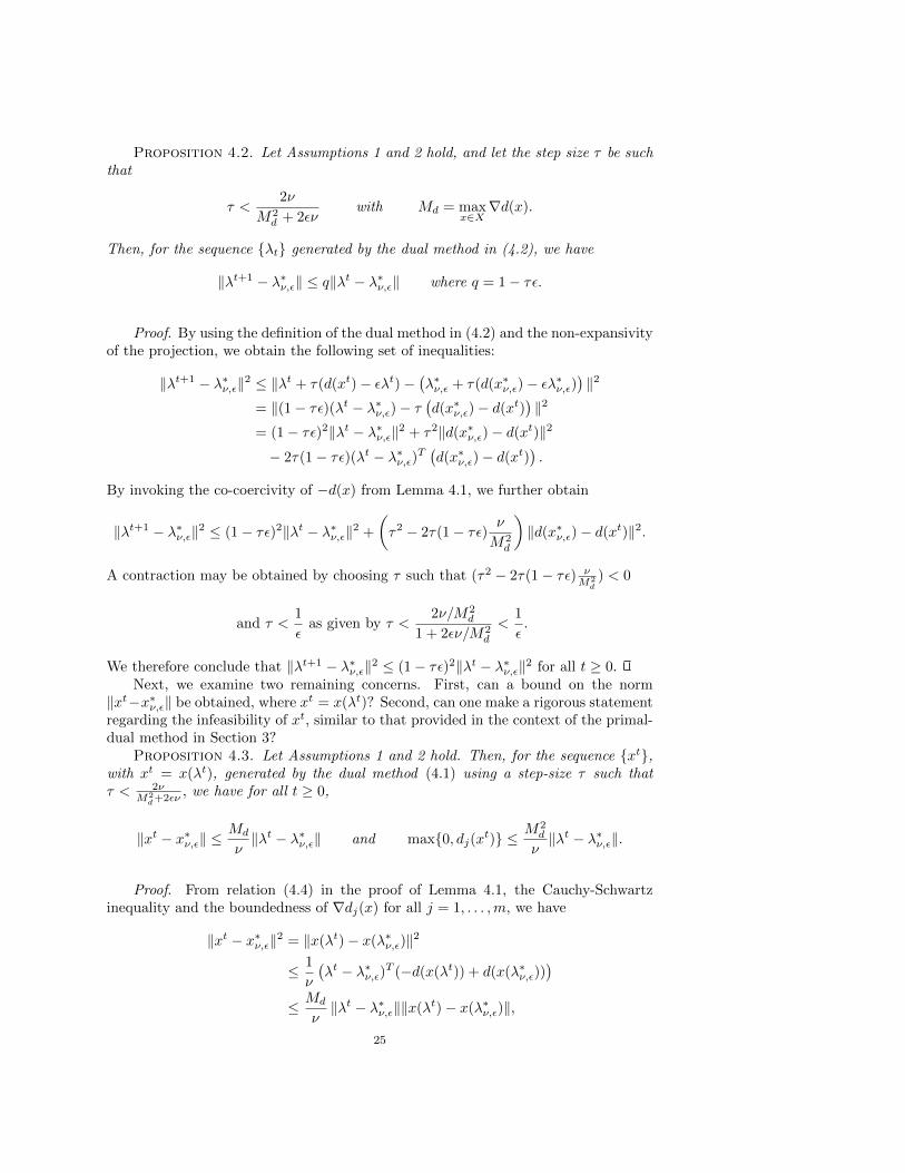
Figure 5.3 illustrates the performance of the primal-dual algorithm in terms of thenumber of iterations required to attain ‖zk− z∗ν,ε‖ < 10−3 as the steplength deviationin primal space αmax − αmin increases. All users employ the same regularizationparameter νi = ν = 0.1 and the dual regularization parameter ε is chosen to be 0.1.The plot demonstrates that, as the deviation between users’ step-sizes increases, thenumber of iteration for a desired accuracy also increases.

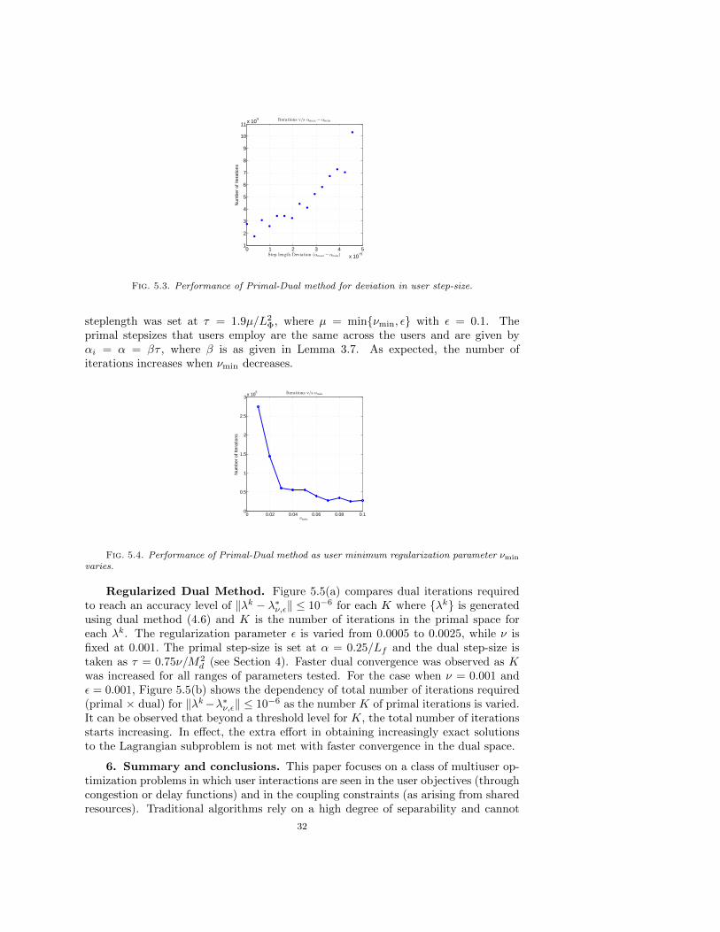
Next, we let each user choose its own regularization parameter νi with uniformdistribution over interval (νmin, 0.1) for a given νmin ≤ 0.1. Figure 5.4 shows theperformance of the primal-dual algorithm in terms of the number of iterations requiredto attain the error ‖zk − z∗V,ε‖ < 10−3 as νmin is varied from 0.01 to 0.1. The dual

31

0 1 2 3 4 5x 10

−5

1

2

3

4

5

6

7

8

9

10

11x 10

4

Step length Deviation (αmax − αmin)

Num

ber

of It

erat

ions

Iterations v/s αmax − αmin

Fig. 5.3. Performance of Primal-Dual method for deviation in user step-size.

steplength was set at τ = 1.9µ/L2Φ, where µ = min{νmin, ε} with ε = 0.1. The

primal stepsizes that users employ are the same across the users and are given byαi = α = βτ , where β is as given in Lemma 3.7. As expected, the number ofiterations increases when νmin decreases.

0 0.02 0.04 0.06 0.08 0.10

0.5

1

1.5

2

2.5

3x 10

5

νmin

Num

ber

of It

erat

ions

Iterations v/s νmin

Fig. 5.4. Performance of Primal-Dual method as user minimum regularization parameter νmin

varies.

Regularized Dual Method. Figure 5.5(a) compares dual iterations requiredto reach an accuracy level of ‖λk − λ∗ν,ε‖ ≤ 10−6 for each K where {λk} is generatedusing dual method (4.6) and K is the number of iterations in the primal space foreach λk. The regularization parameter ε is varied from 0.0005 to 0.0025, while ν isfixed at 0.001. The primal step-size is set at α = 0.25/Lf and the dual step-size istaken as τ = 0.75ν/M2

d (see Section 4). Faster dual convergence was observed as Kwas increased for all ranges of parameters tested. For the case when ν = 0.001 andε = 0.001, Figure 5.5(b) shows the dependency of total number of iterations required(primal × dual) for ‖λk−λ∗ν,ε‖ ≤ 10−6 as the number K of primal iterations is varied.It can be observed that beyond a threshold level for K, the total number of iterationsstarts increasing. In effect, the extra effort in obtaining increasingly exact solutionsto the Lagrangian subproblem is not met with faster convergence in the dual space.

6. Summary and conclusions. This paper focuses on a class of multiuser op-timization problems in which user interactions are seen in the user objectives (throughcongestion or delay functions) and in the coupling constraints (as arising from sharedresources). Traditional algorithms rely on a high degree of separability and cannot

32

8 10 12 14 16 18 201000

2000

3000

4000

5000

6000

7000

8000

primal iterations

dual

iter

atio

nsdual iteration v/s primal iteration

ζ=(0.001,0.0005)

ζ=(0.001,0.001

ζ=(0.001,0.0015))

ζ=(0.001,0.002)

ζ=(0.001,0.0025)

(a)

5 10 15 203

3.5

4

4.5

5

5.5

6x 104

primal iterations

tota

l no.

of i

tera

tions

(b)

Fig. 5.5. Inexact Dual Method: (a) Comparison of dual iterations for a fixed number K ofprimal iterations; (b) Dependency of the total number of primal and dual iterations as the numberK of primal iterations varies.

be directly employed. They also rely on coordination in terms of uniform or equalstep-sizes across users. The coordination requirements have been weakened to variousdegrees in the present work, which considers primal-dual and dual gradient algo-rithms, derived from the fixed-point formulations of the regularized problem. Theseschemes are analyzed in an effort to make rigorous statements regarding convergencebehavior as well as provide error bounds in regularized settings that limited coordi-nation across step-length choices and inexact solutions. Our main contributions aresummarized next:

(1) Regularized primal-dual method: Under suitable convexity assumptions, weconsider a regularized primal-dual projection scheme and provide error boundsfor the regularized solution and optimal function value with respect to theiroptimal counterparts. In addition, we also obtain a bound on the infeasibilityfor the regularized solution. We also show that, under some conditions, themethod can be extended to allow not only for independent selection of primaland dual stepsizes as well as independently chosen steplengths by every userbut also when users choose their regularization parameter independently.

(2) Regularized dual method: In contrast with (1), applying dual schemes wouldrequire an optimal primal solution for every dual step. We show the contrac-tive nature of a regularized dual scheme reliant on exact primal solutions.Furthermore, we develop asymptotic error bounds where for each dual iter-ation, the primal method for solving the Lagrangian subproblem terminatesafter a fixed number of steps. We also provide error bounds for the obtainedsolution and Lagrange multiplier as well as an upper bound on the infeasibil-ity. Finally, we extend these results to the case when each user independentlychooses its regularization parameter.

It is of future interest to consider the algorithms proposed in [17, 19] as appliedto multiuser problem, whereby the users are allowed to implement step-sizes withina prescribed range of values. For this, at first, we would have to develop the errorbounds for the algorithms in [17,19] for the case when different users employ different

33

steplengths.

7. Appendix. Lemma 7.1. Let Assumption 2 hold. Then, for each ν > 0, wehave

0 ≤ f(x∗ν)− f∗ ≤ ν

2(D2 − ‖x∗ν‖2) where D = max

x∈X‖x‖.

Proof. Under Assumption 2, both the original problem and the regularized prob-lem have solutions. Since the regularized problem is strongly convex, the solutionx∗ν ∈ X is unique for every ν > 0. Furthermore, we have

fν(x∗ν)− fν(x) ≤ 0 for all x ∈ X.

Letting x = x∗ in the preceding relation, and using fν(x) = f(x) + ν2‖x‖2 and

f∗ = f(x∗) we get

f(x∗ν)− f∗ ≤ ν

2

(‖x∗‖2 − ‖x∗ν‖2

).

Since x∗ ∈ X solves the original problem and x∗ν ∈ X, we have 0 ≤ f(x∗ν) − f(x∗).Thus, from f∗ = f(x∗), using D = maxx∈X ‖x‖, it follows that 0 ≤ f(x∗ν) − f∗ ≤ν2

(‖x∗‖2 − ‖x∗ν‖2

)≤ ν

2 (D2 − ‖x∗ν‖2).

REFERENCES

[1] A. Beck and M. Teboulle, A fast iterative shrinkage-thresholding algorithm for linear inverseproblems, SIAM Journal on Imaging Sciences, 2 (2009), pp. 183–202.

[2] , Gradient-based algorithms with applications to signal-recovery problems, in ConvexOptimization in Signal Processing and Communications, Y. Eldar and D. Palomar, eds.,Cambridge University Press, 2010, pp. 42–88.

[3] D. P. Bertsekas, Nonlinear Programming, Athena Scientific, Bellmont, MA, 1999.[4] D. P. Bertsekas, A. Nedic, and A. Ozdaglar, Convex Analysis and Optimization, Athena

Scientific, Belmont, MA, 2003.[5] D. P. Bertsekas and J. Tsitsiklis, Parallel and Distributed Computation: Numerical Meth-

ods, Prentice Hall Inc., 1989.[6] R. H. Byrd, M. E. Hribar, and J. Nocedal, An interior point algorithm for large-scale

nonlinear programming, SIAM Journal Optimization, 9 (1999), pp. 877–900 (electronic).Dedicated to John E. Dennis, Jr., on his 60th birthday.

[7] M. Chiang, S. Low, A. Calderbank, and J. Doyle, Layering as optimization decomposi-tion: A mathematical theory of network architectures, Proceedings of the IEEE, 95 (2007),pp. 255–312.

[8] F. Facchinei and J.-S. Pang, Finite-Dimensional Variational Inequalities and Complemen-tarity Problems, vol. 1 and 2, Springer-Verlag Inc., New York, 2003.

[9] F. Kelly, A. Maulloo, and D. Tan, Rate control for communication networks: shadowprices, proportional fairness, and stability, Journal of the Operational Research Society,49 (1998), pp. 237–252.

[10] I. Konnov, Methods for solving multivalued variational inequalities, in At the turn of the20th–21st centuries (Russian), Kazan. Mat. Obs., Kazan, 2003, pp. 68–79.

[11] , Equilibrium models and variational inequalities, Elsevier, 2007.[12] G. Korpelevich, The extragradient method for finding saddle points and other problems,

Matekon, 12 (1976), pp. 747–756.[13] S. Low and D. Lapsley, Optimization flow control, I: Basic algorithm and convergence,

IEEE/ACM Transactions on Networking, 7 (1999), pp. 861–874.[14] A. Nedic and A. Ozdaglar, Subgradient methods in network resource allocation: Rate anal-

ysis, in 42nd Annual Conference on Information Sciences and Systems, CISS, Princeton,2008, pp. 1189–1194.

[15] , Approximate primal solutions and rate analysis for dual subgradient methods, SIAMJournal on Optimization, 19 (2009), pp. 1757–1780.

34

[16] , Subgradient methods for Saddle-Point problems, Journal of Optimization Theory andApplications, 142 (2009), pp. 205–228.

[17] A. Nemirovski, Prox-method with rate of convergence O(1/T) for variational inequalities withlipschitz continuous monotone operators and smooth convex-concave saddle point problems,SIAM Journal On Optimization, 15 (2004), pp. 229–251.

[18] Y. Nesterov, Smooth minimization of non-smooth functions, Mathematical Programming,Ser. A, 103 (2005), pp. 127–152.

[19] Y. Nesterov, Dual extrapolation and its applications to solving variational inequalities andrelated problems, Mathematical Programming, 109 (2007), pp. 319–344.

[20] J.-S. Pang and D. Chan, Iterative methods for variational and complementarity problems,Mathematical Programming, 24 (1982), pp. 284–313.

[21] B. T. Polyak, Introduction to Optimization, Optimization Software, May 1987.[22] X. Qin and R. Berry, Distributed power allocation and scheduling for parallel channel wireless

networks, in Third International Symposium on Modeling and Optimization in Mobile, AdHoc, and Wireless Networks, 2005. WIOPT, 2005, pp. 77–85.

[23] S. Shakkottai and R. Srikant, Network optimization and control, Foundations and Trendsin Networking, 2 (2007), pp. 271–379.

[24] M. Solodov and P. Tseng, Modified projection-type methods for monotone variational in-equalities, SIAM Journal on Control and Optimization, 34 (1996), pp. 1814–1830.

[25] R. Srikant, Mathematics of Internet Congestion Control, Birkhauser, 2004.[26] P. Tseng, On accelerated proximal gradient methods for convex-concave optimization. submit-

ted to SIAM Journal on Optimization, 2008.[27] J. Tsitsiklis, Problems in decentralized decision making and computation, PhD thesis, Mas-

sachusetts Institute of Technology, 1984.[28] H. Uzawa, Iterative methods in concave programming, Studies in Linear and Nonlinear Pro-

gramming, (1958), pp. 154–165.[29] H. Yin, U. Shanbhag, and P. Mehta, Nash equilibrium problems with congestion costs and

shared constraints, in Proceedings of the 48th IEEE Conference on Decision and Control,2009 held jointly with the 2009 28th Chinese Control Conference. CDC/CCC 2009., 2009,pp. 4649–4654.

[30] H. Yin, U. V. Shanbhag, and P. G. Mehta, Nash equilibrium problems with congestion costsand shared constraints, To appear in IEEE Transactions of Automatic Control (July 2011),(2009).

35