helicopter flight simulation motion platform requirements · · 2013-08-30helicopter flight...

NASA/TP-1999-208766

Helicopter Flight Simulation Motion Platform

Requirements

Jeffery Allyn Schroeder

Ames Research Center, Moffett Field, California

National Aeronautics and

Space Administration

Ames Research Center

Moffett Field, California 94035-1000

July 1999

https://ntrs.nasa.gov/search.jsp?R=19990080926 2018-05-29T12:34:03+00:00Z

NASA Center tbr AeroSpace Information

7121 Standard Drive

Hanover, MD 21076-1320

(301) 621-0390

Available from:

National Technical Information Service

5285 Port Royal Road

Springfield, VA 22161(703) 487-4650

Contents

Summary ......................................................................................................................................... 1

1. Introduction .................................................................................................................................. 3

Background ............................................................................................................................... 3

Purpose of This Report ............................................................................................................... 10

Approach ................................................................................................................................. 10

Contributions ........................................................................................................................... 10

Outline .................................................................................................................................... 11

2. The Vertical Motion Simulator ........................................................................................................ 13

General Description .................................................................................................................... 13

Performance Characteristics ......................................................................................................... 13

3. Yaw Experiment ............................................................................................................................ 15

Background ............................................................................................................................... 15

Experimental Setup .................................................................................................................... 15

Results .................................................................................................................................... 19

4. Vertical Experiment I: Atltitude Control ............................................................................................ 31

Background ............................................................................................................................... 31


Results .................................................................................................................................... 34

5. Vertical Experiment II: Compensatory Tracking .................................................................................. 41

Background ............................................................................................................................... 41

Experimental Setup .................................................................................................................... 4 !

Results .................... ."............................................................................................................... 42

6. Vertical Experiment III: Altitude and Altitude-Rate Estimation ............................................................... 49

Background ............................................................................................................................... 40


Results: Objective Performance Data ............................................................................................. 5 l

7. Roll-Lateral Experiment .................................................................................................................. 55

Background ............................................................................................................................... 55


Results .................................................................................................................................... 57

8. Discussion of Overall Results .......................................................................................................... 63

General Discussion .................................................................................................................... 63

Proposed Fidelity Criteria versus Results of Previous Rcsearch .......................................................... 63

A General Method for Configuring Motion Systems ........................................................................ 66

iii

9.Conclusions.................................................................................................................................69

Summary.................................................................................................................................69RecommendationsforFutureWork...............................................................................................69

AppendixA--HumanMotionSensingCharacteristics..............................................................................71

AppendixB--HeightRegulationAnalysiswithPreviousModel ................................................................ 75

Appendix C--Example of Repeated-Measures Analysis ............................................................................ 81

Appendix D--Review of Cooper-Harper Handling Qualities Rating Scale .................................................... 83

References ........................................................................................................................................ 85

iv

Helicopter Flight Simulation Motion Platform Requirements

JEFFERY ALLYN SCHROEDER


Summary

Flight simulators attempt to reproduce actual flight pilot-

vehicle behavior on the ground reasonably and safely. This

reproduction is especially challenging for helicopter flight

simulators, which is the subject of this work, for the pilot

is often inextricably dependent on external cues for pilot-

vehicle stabilization. One of the important simulator cues

is platform motion; however, its required fidelity is not

known. Cockpit motion effects on pilot-vehicle

performance, on pilot workload, and on pilot motion

perception were examined in several experiments in order

to determine the required motion fidelity for helicopter

flight simulation. In each experiment, a large-

displacement motion platform was used that, for some

configurations, allowed pilots to fly tasks with a one-to-

one correspondence between the motion and visual cues.

In all evaluations, representative helicopter math models

were employed, and in two cases a specially developed

model from AH-64 Apache flight test data was used.

Platform motion characteristics were modified to give

motion cues varying from full motion, relativc to the

visual scene, to no motion. Four of the six rigid-body

degrees of freedom were explored: roll rotation, yawrotation, lateral translation, and vertical translation. The

pitch rotation and longitudinal translation degrees of

freedom remain for future work; however, it was hypothe-

sized that thcir requirements mirror those of roll rotation

and lateral translation. Several key results were found fromthe evaluations. First, lateral and vertical translational

motion platform cues had significant effects on simulation

fidelity. Their presence improved pilot-vchiclc

performance, reduced pilot physical and mental workload,

and improved pilot opinion of how faithfully the simula-

tions represented flight. Second, yaw and roll rotational

motion platform cues were not as important as the lateral

and the vertical translational platform cues. In particular,

the yaw rotational motion platform cue did not appear at

all useful in improving performance or reducing workload.

Third, when the lateral translational motion platform cues

were combined with visual yaw rotational cues, pilots

believed they were physically rotating when the motion

platform was not rotating. Thus, an overall efficiency inthe use of motion cues can be obtained by combining

only the lateral translational platform cues with

satisfactory visual cues. Fourth, vertical and roll/lateral

specifications were revised and validated that provide

simulator users with a prediction of motion fidelity based

on the frequency-response characteristics of their motion

control laws. Fifth, vertical platform motion affected pilot

estimates of steady-state altitude during altitude reposi-

tionings. This refutes the view that pilots estimatealtitude and altitude rate in simulation solely from visualcues. Since these studies have shown that translational

motion platform cues had more important effects on

simulation fidelity than did rotational cues, an alternative

to today's hexapod platform design is suggested which

emphasizes the translational cues. And sixth, the

combined results led to a general method for configuring

helicopter motion systems as well as for developingsimulator tasks that more likely represent actual flight.

The overall results can servc as a guide to future simulator

designers and to today's operators.

1. Introduction

Background

Purpose of Flight Simulation

Flight simulation had its origins near to those of powered

flight itself (ref. 1). Since then, simulation has been used

principally for two distinct disciplines in aviation:

training and research and development. However, flight

training is its most frequent application, in which it is

used primarily to reduce cost and increase safety. Almost

all of the major airlines use flight simulation today

whenever they can receive a training credit for doing so.

This is because an hour in the simulator is less expensive

than an hour in the airplane. For example, a B-747 aircraft

costs about $12,500 per hour to operate versus about

$750 per hour for a 747 simulator (ref. 2).

These cost reductions are put to both training and

retraining uses. The Federal Aviation Administration

(FAA) will certify certain simulators such that, with only

simulator training, a new pilot may fly the actual aircraft

for the first time carrying passengers (ref. 3). Once a pilot

is qualified in a particular aircraft, mandatory periodic

proficiency checks are then conducted in the simulator.

Some of these latter checks may also include recovery

from failures or unusual attitudes (ref. 4). This training is

considered too hazardous to perform in the actual aircraft.

Although the previous discussion relates to fixed-wing

transport training, a similar use for flight simulation is

under way for helicopter training. For helicopters,

however, less is known about what level of fidelity isneeded for these simulators. The FAA has released an

Advisory Circular suggesting fidelity requirements for

helicopter simulators (ref. 5), but little data exist to

support the requirements. Its development started with the

fixed-wing Advisory Circular (ref. 3), and the specifica-

tions in most areas were made more stringent owing to

the greater dependency a pilot places on external cues in

helicopter flight than in fixed-wing flight.

The other principal use of flight simulation is for research

and development. When an aircraft system, or component,reaches a mature level of development, it is often evalu-

ated by a pilot in simulation. These simulations may beused to evaluate a new vehicle's handling qualities or the

functionality of a new system component in a morerealistic and safer environment prior to flight testing.

Flight simulation results may also yield a final product,

such as data for a handling-qualities specification. Finally,

flight simulation may be used to determine the causalfactors in an accident. An accident scenario can be

duplicated in order to hypothesize crew action in responseto events.

In the above instances, flight simulation attempts to

imitate flight. Figure 1 illustrates the key components of

simulation and flight. In flight, a pilot receives cues that

indicate vehicle motion in three main ways. First, motion

is perceived from visual cues with the eyes. Second, the

pilot perceives motion from the vehicle's acceleration.

Third, the pilot can infer, or predict motion, via the

kinesthetic force and position cues that the vehicle's force-

feel system provides. The latter is an often neglected, but

important, cueing source (refs. 6, 7).

In contrast, the pilot seldom receives any of these cues

accurately in simulation. The aircraft is now represented

by a mathematical aircraft model, which is likely to

contain inaccuracies. The visual system, which is

typically computer generated, does not provide the cueingrichness of the real world. The simulator visual field of

view is usually less than that of the vehicle, and the

visual acuity provided today is incapable of rendering

20/20 vision. The vehicle's force-feel system is usually

the easiest to replicate, although matching the nonlinear

effects (friction, free-play, and hysteresis) and the inertia

characteristics can be challenging. This challenge results

both from a surprising lack of flight data and from

simulator force-feel system limitations. And because the

simulator displacements are constrained, the motion

system can typically provide only a subset of the in-flightaccelerations. It is the motion system that is the focus of

this report.

Of the above cueing sources, only the motion platform

has practical hard technological limits in its capability to

reproduce the in-flight cues. Thus, in light of those hardlimits and the associated costs of providing them, estab-

lishing reliable motion fidelity requirements is warranted.

This is especially true for helicopters, since the pilot often

stabilizes the pilot-vehicle system, and this stabilization

is only possible via feedback from the simulator's cueing

systems.

The Role of Platform Motion in Flight Simulation

The role of platform motion has been the subject of greatdebate. Some researchers and users believe in the extreme

that no platform motion is necessary. Some believe in the

exact opposite. As pointed out by Boldovici (ref. 8),

"Debates about whether to buy motion bases often include

anecdotes, misinterpretation of research results, and

incomplete knowledge of the research issues that underliethe research results." Toward understanding the role of

motion in flight simulation, the arguments for the

support of each of these views are given below.

Task

Stickforce

cue8I_ Force-feel I ._[

Pilot L_ dynamics ] I "- I

T I Stick displacementcues IReal-world motion cues

Aircraft

Real-world visual cues

v

Flight

Simulator

stickforce

I cues I Simulated I IPilot _ force-feel

"n'm'°"I I Idisplacement cues I

Simulator motion cues

Simulator visual cues

Aircraftmodel

Motion

system

Visualsystem

v

Simulation

Figure 1. Flight versus simulation.

The Case Against Platform Motion. Cardullo

cites many of the reasons users either do not employ

motion or believe it is unnecessary (ref. 9). First,

platform motion usually does not have the face validity

that a simulation component such as the visual system

does. Face validity is defined as a seamless one-to-one

correspondence with the real world. Some subsequently

argue that since the true motion environment cannot be

duplicated faithfully, a subset of it should not be

presented, for the cues are incorrect. It is also argued that

providing platform motion is not cost effective. Finally,

opponents of motion note that transfer-of-training studies

have found no basis for a motion requirement. In

particular, the U.S. Air Force's

standard view for training is that motion is not required in

the simulation of any aircraft with centerline thrust.

Roscoe (ref. 10) states that "Complex cockpit motion,

whether slightly beneficial or detrimental on

balance.., has so little effect on training transfer thatits contribution is difficult to measure at all." The two

studies most often cited showing that motion did not have

a training benefit for several tasks are those by Waters

et al. (ref. 11) and Gray and Fuller (ref. 12). However,

Cardullo points out that these two studies have largely

been discredited because of the poor experimental

apparatus used in each study (ref. 9). In particular, the

motion systems had large motion platform delays.

4

Boldovici(ref.8),inanextensivereviewfortheU.S.Army,presentsseveralreasonsfornotusingmotionplatforms:(1)theabsenceofsupportingresearchresults,(2)possiblelearningofunsafebehaviorbasedonincorrectplatformcueing,(3)achievementofgreatertrainingtransferbymeansotherthanmotioncueing,(4)undesir-ableeffectsofpoormotionsynchronization,(5)direct,indirect,andhiddencosts,(6)alternativestomotionbasesforproducingmotioncueing(e.g.,g-seats,pressuresuits),and(7)benignforceenvironments.

Poormotionsynchronization,whichdoesnothaveaprecisedefinition,hascausedsomepilotstoexperiencesimulatorsickness.Thisdiscomfortaffectsboththepilot'sperformanceandhisacceptanceofasimulator.Surprisinglythediscomfortcanlast,orevendevelop,hoursafterthesimulatorsession.TheU.S.Navyhasrecommendedthatmotionbasesbeturnedoffif sicknessdevelops;however,thatrecommendationnotesthatsomecrewsalsobecomesickintheactualvehicle(ref.13).Somebranchesofthearmedservicesrequireawaitingperiodbetweenasimulatorsessionandflight.

Finally,severalresearchershavedefinedtasksforwhichmotiondoesnotseemtoaddbenefit.Hunteretal.(ref.14)andPuigetal.(ref.15)indicatethatmotiondoesnotseemtobeverybeneficialfortasksinwhichthepilotcreateshisownmotion.Suchinstanceswouldbefortrackingtasksinadisturbance-freeenvironment.TheCaseFor PlatformMotion.Hallattemptstodeterminewhenplatformmotionisandisnotimportant(ref.16).Hecontendsthatnon-visualcuesareoflittleimportanceforprimarilyopen-loop,lowpilot-vehiclegain,lowworkloadmaneuverswithstrongvisualcues.However,healsostatesthatmotioncuesaremoreimportantwhenthepilotworkloadincreases,whenthepilot-vehiclegainrises,orwhenthevehiclestabilitydegrades.Thelattercertainlyoccursinhelicoptersimulation.

ShowaherandParrisconductedastudyinwhichpilotshadtorecoverfromanengine-outduringtakeoffinaKC-135aircraft(ref.17).Theyshowedthattheadditionofmotionsignificantlyreducedtheamountofyawactivityduringanengine-outwhencomparedtotheno-motioncase.Inthesamestudy,theyalsoshowedthattheadditionofmotionaffectedinexperiencedpilots'abilitytoperformprecisionrollingmaneuvers,butthattheadditionofmotionhadnosignificanteffectonexperiencedpilotsforthesametask.

Youngshowedthatplatformmotionreducedthepilot'sresponsetimetoafailureordisturbancewhileonaglidepathcomparedtotheno-motioncase(ref.18).Inthesamepaper,resultswerepresentedshowingthatwhenhelicopterpilotsandhighlytrainednon-pilotshoveredan

unaugmentedhelicoptermodel,theirperformancesignifi-cantlyimprovedwiththeadditionofmotion.Performancedidnotimproveforthemoderatelytrainednon-pilots.

HosmanandvanderVaart(ref.19)foundthatperformanceimprovedwithmotioninrollforbothdisturbancerejectionandtrackingoverthatoftheno-motioncase.However,therollmotioninthiscaseincludedthespuriouslateralspecificforcecuesowingtothelackofsimulatortranslationalmotionavailabletoaccountforcoordination.

OneofthefewstudiesthathasexaminedtheperformanceeffectsoffullmotionversusnomotionwasperformedfortherollaxisbyMcMillanetal.(ref.20).Thatstudyalsoshowedsignificantimprovementintracking,butlittleimprovementinatransfer-of-trainingmetricwhenfullmotionwaspresentovertheno-motioncase.SimilarresultswerepresentbyLevisonetal.(ref.21).

Boldovici(ref.8),inhisbalancedpresentationonbothsidesofthemotionargument,givesasetofreasonsforemployingmotionplatforms:(1)toreducetheincidenceofsimulatorsickness(notethatthisargumentisusedbothforandagainstmotion),(2)users'andbuyers'acceptanceofimprovedvalidity,(3)trainees'motivation,(4)tolearnhowtoperformtime-constraineddangeroustasks,and(5)toovercometheinabilitytoperformsometaskswithoutmotion.

Fordifficultcontroltasks,earlystudiesshowedthatmotionallowsapilottoformthenecessaryleadcompen-sationmorereadilywithaccelerationcuesthanwiththevisualdisplaysalone(refs.18,22).Forstabilizationtasksapilotwilloftenusethisleadcompensationtoreducetheopen-loopsystemphaselossandthusallowanincreaseinthepilot-vehicleopen-loopcrossoverfrequencytoapointhigherthanthatachievedwithoutmotion(ref.23).Thisincreasedcrossoverfrequency,withthesameorbetterphasemargin,yieldstrackingperformancemoreakintothatof flight.

Interestingly,theFAAhasbeenastrongsupporterofplatformmotion.Indeed,if adeviceistobecalledasimulatorbytheFAA,it musthavemotion.If adevicedoesnothavemotion,thentheFAAtermsit "aflighttrainingdevice"(refs.3,5).

Developing Requirements for Motion

Since instances have clearly arisen in which the addition

of platform motion shows significant benefits, the

question remains "For those instances, what are the

motion requirements?" Defining the necessary require-ments for the quality, or fidelity, of that motion has been

difficult. The fact that requirements are not known is

evidentfromthefollowingquotesfromtheliterature."Unfortunately,explicitdefinitionsof'valuable'motionfidelity,forspecificresearchortrainingobjectives,remainforthemostpartundetermined"(ref.24)."Formalexperimentstodetermineacceptable attenuation and phase

lag of the force vector are limited in scope..."(ref. 25). "Future research topics in the area of flight

simulation techniques should encompass minimum

essential visual and motion cueing requirements for a

particular flying mission" (ref. 2).

Although definitive answers regarding necessary motion

requirements do not exist, regulators still suggest which

motion degrees of freedom may be useful. These sugges-

tions depend on the level of simulator sophistication

desired by the user. For instance, the FAA specifies two

levels of motion sophistication for helicopter flight

simulators: full six-degrees-of-freedom motion, and three-

degrees-of-freedom motion (ref. 5). For the latter, the

nominal three degrees of freedom are pitch, roll, and

vertical. If degrees of freedom different from these are

selected by a user, they must be qualified by the FAA on a

case-by-case basis. Although the selection of the pitch,

roll, and vertical degrees of freedom is reasonable, evidence

to support the selection of these axes or any set of axes is

lacking.

Even though existing motion criteria are incomplete,however, considerable research has been performed. To

divide and conquer the problem, the six degrees of freedom

are often broken into two categories: rotational motion

and translational motion. But even at this high level,

differences in opinion exist on the relative cueing impor-

tance of these two categories. For example Stapleford

et al. (ref. 26) state, for tracking, "Translational motion

cues appear to be generally.less important than rotational

ones, although linear motion can be significant in specialsituations." Young states "For most applications, simu-

lation of vehicle angular motions is more important than

translational simulation" (ref. 18). In contrast, the

concluding remarks of Bray (ref. 27) state, "For largeaircraft, due to size and to the basic nature of their

maneuvering dynamics, the cockpit lateral translationalacceleration cues appear to be much more important thanthe roll acceleration cues. There was the indication that

this observation might be extended to the generalization

that, in each plane of motion, the linear cues are muchmorc valuable than the rotational cues."

Reasons for these differences of opinion at a high level are

unclear and point to the need for additional research. But

before the appropriate directions for the additional research

can be determined, a careful review of past work is

warranted. Those analytical and experimental efforts that

havc addressed motion requirements are discussed below.

Analytical Motion Research. Many decisions are

made during both the design and development of a

particular simulation. All of the components shown in

figure 1 must be selected, and their characteristics must be

specified. If an analytical model was available that

accounted for the fidelity effects of these components, then

one could inexpensively make performance trade-offs to

optimize both the cost and utility of a simulator system.

So, a good analytical model would have great use.

Although the dynamics of the non-piloted components of

figure 1 are straightforward, the difficulty facing the

modeler is the pilot block. Pilots are often adaptive,

nonlinear, and inconsistent, and modeling their input/

output characteristics is a challenge. A possible break-

down of the key processes carded out by a pilot is shown

in figure 2. These key processes are sensation, perception,

and compensation. The general characteristics of these

processes are discussed next, because knowledge of themis relevant to the experimental designs presented in latersections.

RemnantSimulator

Pilot : stick

Task force

demandsI

--I_ I CompensationI

I

I Perception [I

I Sensation ]

Simulator

visual, motion,

and stick cues

Figure 2. Top-level pilot model.

The sensation block in figure 2 is often used as the

starting point when motion requirements are hypothesized,

and a large database exists on human motion-sensingcharacteristics (refs. 28-36). The details of the human

motion sensing systems are given in appendix A, but four

key points are made here. First, the bandwidth of the total

human motion sensory system encompasses the typical

pilot-vehicle range of frequencies (0.1-10 rad/sec). Second,

for the experiments that are subsequently described, thethresholds of human motion sensors were exceeded;

however, the literature acknowledges that motion-sensing

thresholds differ among individuals and that thcy depend

on whether the subject is active or passive during the

motionstimulus(ref.36).Third,previousincorporationofthemotiondynamicsandthresholdsintomodelsofapilot-vehiclesystemhasnotresultedinanimprovedabilitytomodelpilot-vehiclebehavior(ref.35).Finally,previouseffortstogenerateanintegratedmotioncueingmodelhaveconcludedthatadditionalexperimentsneedtobeconductedbeforethatgoalcanbeaccomplished(ref.31).

Oncethecuesaresensed,theperceptionblockoffigure2comesnext.Atthispoint,anintegratedperceptualprocesslikelyoccurs,buthowit isaccomplishedisnotknownexactly.Onehastoknowhowalloftheexternalcues(visual,kinesthetic,andtactile)aresummedtodevelopthepilot'sperceptionofmotion.Unfortunately,littleisknownabouthowthesecuesaffectmotionperception,andfurthercarefulexperimentsarerequiredtoexploretheperceptualinteractionsthatoccuramongthesecues.

Afterthepilothasdevelopedanestimateofthevehiclestatefromtheoutputoftheperceptionblock,compensa-tionis thenappliedtothisstatevector.Fundamentally,itisknownthatthepilotappliescompensationnecessarytohave"integrator-like"or"K/s-like"characteristicsinthecrossoverregionofthepilot-vehicleopen-loopcombina-tion(ref.37).Todothis,apilotwill typicallyprovideupto1secofleadbeforehisestimateofataskworkloadisdegraded.

ApplicationoftheaboveconceptsispresentedinappendixB,whichgivesdetailsofastructuralpilotmodelfortheverticalaxisexperimentdescribedinsection4.It isshownthatthemodelcapturesthegeneralclosed-loopperformancetrends.However,itunderpredictsthemagnitudeofthesetrendstothepointthatit suggestsnofidelitydifferencesshouldexistwhen,infact,theydoexist.Inaddition,themodelisincomplete,forit doesnotaccountforthegainonmotionplatformacceleration.

Tosummarize,acredibleanalyticalmodeldoesnotyetexistforflightsimulation.Moreexperimentaldataareneededtodevelop and refine the model further. The experi-

ments that have been performed to date are discussed next.

Experimental Motion Research. Many previous

experiments have contributed toward the development of

motion-fidelity requirements. Although some of the data

from these previous studies may be correlated, differences

in visual and motion systems, tasks, and vehicle dynamics

typically prevent the consistent understanding and

development of motion-fidelity criteria. Below, key resultsof both rotational and translational experiments are

presented.

Experimental Rotational Criteria. Staplefordet al. examined the effects of roll and roll-lateral motion

on a pilot's ability to track a target during a disturbance

(ref. 26). Using both a tracking and a disturbance input,

some key aspects of how the pilot closes the visual and

motion feedback loops were presented. They suggested

that angular cues be accurate in the 0.5-10 rad/sec range;

however, "accurate" was not precisely defined.

Bergeron evaluated the effects of attenuating only the

motion filter gain in the angular degrees of freedom

(ref. 38). For the highly stabilized vehicle that was

simulated, the results suggested that motion has no effect

on the performance of single-axis stabilization tasks.

Motion effects became evident only when simultaneous

control of two angular axes was required. Presenting as

little as 25% of the full motion produced results

comparable to those for full motion.

In the Netherlands, van Gool suggested that second-order

pitch and roll high-pass filters with break frequencies of

0.5 rad/sec appear adequate (ref. 39). This result was for

stabilizing the pitch and roll attitude of a DC-9 on

approach. Both the high-frequency gain and damping ratio

of the motion filter were unity in all of van Gool's

motion configurations.

Cooper and Howlett examined five tasks with a helicopter

model in an attempt to determine motion fidelity require-

ments for a particular six-degrees-of-freedom hexapod

motion platform (ref. 40). They made the point that toachieve maximum results from a simulator, the structure

and values of the high-pass motion filters need to betailored for the task while staying within the platform

excursion limits. Although motion amplitude can be

reduced by either reducing the motion filter gain or the

time-constant, their experience had been that it was betterto use the combination of both rather than reducing onlythe time-constant. Their tentative conclusion was that it

was best to use a gain of 0.8 in pitch and roll with a time-constant of 4 sec.

Using a fixed-wing model, the effects of roll-only motion

were examined by Jex et al. (ref. 41). Their recommenda-

tion was to provide the pilot with accurate roll-rate

motion cues at frequencies above 0.5-1.0 rad/sec with a

first-order high-pass filter. A filter time-constant of2-3 sec was recommended. Here, the word "accurate"

included the allowance of a 0.54).7 gain on the filter.

Not providing the initial full roll-rate cue was deemed

acceptable.

Shirachi and Shirley used a model of a Boeing 367

transport for a disturbancc-rejection task in roll (ref. 42).

The simulator motion platform had sufficient lateral

translational displacement to coordinate the rolling

maneuvers. The results suggested that if the high-

frequency gain on the roll high-pass filter was lower than

about 0.5 performance would approach that of no motion.

Thisgainlimitationwasdeemedacceptablewithasecond-orderhigh-passfilterbreakfrequencyof0.7rad/sec.

Brayfoundthatforalargetransportaircraftwithfullrollgain,motionfilterbreakfrequenciesof0.5rad/seccausedslightcontradictionsinthevisualandrollmotions(ref.27).Increasingthebreakfrequencyto1.0or1.4rad/secresultedinareductionofsomepilots'abilitytostabilizetheDutchrollmotions.

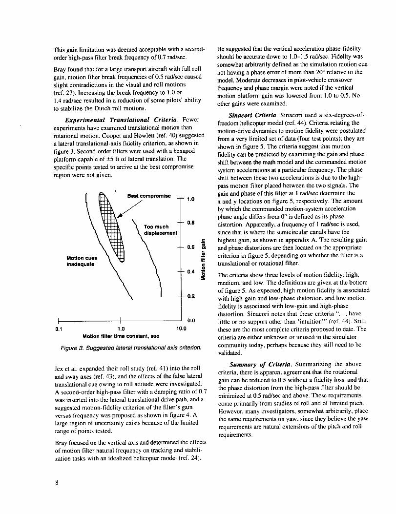
Experimental Translational Criteria. Fewer

experiments have examined translational motion than

rotational motion. Cooper and Howlett (ref. 40) suggesteda lateral translational-axis fidelity criterion, as shown in

figure 3. Second-order filters were used with a hexapod

platform capable of +_5 ft of lateral translation. The

specific points tested to arrive at the best compromise

region were not given.

I0.1

Motion cuesinadequate

" Best compromise .

J

I1.0

Motion filter time constant, sec

10.0

1.0

0.8

.¢_I00.6 m

0.4

0.2

0.0

Figure 3. Suggested lateral translational axis criterion.

¢:0

Jex et al. expanded their roll study (ref. 41) into the roll

and sway axes (ref. 43), and the effects of the false lateraltranslational cue owing to roll attitude were investigated.

A second-order high-pass filter with a damping ratio of 0.7

was inserted into the lateral translational drive path, and a

suggested motion-fidelity criterion of the filter's gainversus frequency was proposed as shown in figure 4. A

large region of uncertainty exists because of the limited

range of points tested.

Bray focused on the vertical axis and determined the effectsof motion filter natural frequency on tracking and stabili-

zation tasks with an idealized helicopter model (ref. 24).

He suggested that the vertical acceleration phase-fidelity

should be accurate down to 1.0-1.5 rad/sec. Fidelity was

somewhat arbitrarily defined as the simulation motion cue

not having a phase error of more than 20 ° relative to the

model. Moderate decreases in pilot-vehicle crossover

frequency and phase margin were noted if the vertical

motion platform gain was lowered from 1.0 to 0.5. No

other gains were examined.

Sinacori Criteria. Sinacori used a six-degrees-of-

freedom helicopter model (ref. 44). Criteria relating the

motion-drive dynamics to motion fidelity were postulated

from a very limited set of data (four test points); they are

shown in figure 5. The criteria suggest that motion

fidelity can be predicted by examining the gain and phaseshift between the math model and the commanded motion

system accelerations at a particular frequency. The phaseshift between these two accelerations is due to the high-

pass motion filter placed between the two signals. The

gain and phase of this filter at 1 rad/sec determine the

x and y locations on figure 5, respectively. The amount

by which the commanded motion-system acceleration

phase angle differs from 0° is defined as its phasedistortion. Apparently, a frequency of I rad/sec is used,since that is where the semicircular canals have the

highest gain, as shown in appendix A. The resulting gain

and phase distortions are then located on the appropriatecriterion in figure 5, depending on whether the filter is atranslational or rotational filter.

The criteria show three levels of motion fidelity: high,

medium, and low. The definitions are given at the bottom

of figure 5. As expected, high motion fidelity is associated

with high-gain and low-phase distortion, and low motion

fidelity is associated with low-gain and high-phasedistortion. Sinacori notes that these criteria "... have

little or no support other than 'intuition'" (ref. 44). Still,

these are the most complete criteria proposed to date. Thecriteria are either unknown or unused in the simulator

community today, perhaps because they still need to bevalidated.

Summary of Criteria. Summarizing the above

criteria, there is apparent agreement that the rotational

gain can be reduced to 0.5 without a fidelity loss, and that

the phase distortion from the high-pass filter should be

minimized at 0.5 rad/sec and above. These requirements

come primarily from studies of roll and of limited pitch.

However, many investigators, somewhat arbitrarily, place

the same requirements on yaw, since they believe the yaw

requirements are natural extensions of the pitch and roll

requirements.

- 0.0

"The Leans"0.2

0.4 _

o.6 "_Travellimits Region of uncertainty

exceeded0.8

e Force"I I 1.0

0.0 0.2 0.4 0.6 0.8 1.0

Sway high-pass filter natural frequency, rad/sec

Figure 4. Sway motion fidelity criterion (ref. 43).

I0.0

I0.2

Specific force- -100

• 80

Low

6O

Medium

I I0.4 0.6

Gain @ 1 rad/eec

- - 40

. . 20

High

Low

Rotational velocity

Medium

High

0 I I I0.8 1.0 0.0 0.2 0.4 0.6 0.8

Gain @ 1 rad/sec

100

8O

6O

4O

2O

01.0

Q)

fJQ)

13

v-

@r-

.o

O

.m"O

bltllJ=

¢L

HighMediumLow

Motion sensations are close to those of visual flight

Motion sensation differences are noticeable but not objectionable

Differences are noticeable and objectionable, loss of performance, disorientation

Figure 5. Sinacori motion-fidefity criteria (ref. 44).

9

For the translational motion fidelity, the agreement is less

apparent. The data for the translational requirements are

primarily from lateral translational-axis experiments, withsome data from the vertical axis. There are also disagree-ments as to whether these translational cues are more

important that the rotational cue, or vice versa.

Since motion fidelity has not been thoroughly examined

in all axes, it is possible that some motion degrees offreedom are redundant with the other simulator cues that

also allow motion perception. If a motion degree of

freedom is unnecessary, then a savings might be realized

as a result of the reduced complexity in the design,

development, and operation of flight simulators. If a

savings benefit is not chosen by a manufacturer, at least

an operator would know not to concentrate on tuning the

motion in an unnecessary degree of freedom.

An answer to "How much platform motion is enoughT' is

likely to be vehicle and task dependent. Vehicles that rely

greatly on the pilot for stabilization, such as helicopters,will have more stringent platform-motion requirements

than vehicles that do not depend on the pilot for stabili-

zation. As such, this report focuses on the former, more

stringent case.

Purpose of This Report

The purpose of this report is to develop reasonable

guidelines for the use of motion in helicopter simulations.

Areas in which weak guidance exists on how to employ

key motion cues will be strengthened. Specifically, it will

be first determined if yaw requirements are a natural

extension of pitch and roll requirements. Second, the

fidelity effects of vertical motion and their interaction withvisual cues in altitude control will be determined. Finally,

requirements for the relative magnitudes of roll and lateral

translational motion will be investigated.

Approach

Although platform-motion research has been conducted

previously, the approach used here is, perhaps, morevalid. Therc are several reasons for this greater validity.

First, the world's largest displacement flight simulator

was used in all of the experiments. Use of this experi-mental device allows selected flying tasks to be duplicated

faithfully. That is, the math model, the visual cues, andthe motion cues can be matched as a baseline, and then the

effects of altering motion can be subsequently determined.

Second, representative helicopter math models were used,with onc model identified from flight test. This

approach allows helicopter-specific requirements to bedetermined. Third, highly experienced test pilots were used

as subjects, and their insightful comments allow confident

extrapolations from simulation to flight. Finally, the

results were corroborated with both objective and subjec-

tive data. In most cases, enough data were collected to

allow the measures to be quantified statistically, an

advantage that limited facility-use time often does notallow.

These methods should provide a high degree of confidence

in the results. They were applied in order to the yaw,

vertical, roll, and lateral translational degrees of freedom.

Motions in the yaw and vertical axes were examined first,

because these motions are the simplest. That is, the

gravity vector remains aligned relative to the cockpit for

these motions. Next, the coupled roll and lateral axes were

explored. These motions are coupled, since the gravity

vector rotates relative to the cockpit. The coupled pitch

and longitudinal axes have been left for future work;

however, the requirements in pitch and longitudinal are

not expected to differ substantially from those of roll andlateral.

Contributions

1. The results indicate that yaw rotational platform

motion has no significant effect in hovering flight

simulation. For three tasks that broadly represented

hovering flight, the addition of yaw-rotational motion

yielded insignificant changes in pilot-vehicle posi-

tioning performance, pilot control activity, pilots'

rating of required control compensation, and pilots'

opinion of motion fidelity.

2. Lateral translation of the motion platform has a

significant effect on hovering flight simulation. For

three tasks that broadly represent hovering flight, theaddition of lateral translational motion improved

pilot-vehicle positioning performance, reduced pilot

control activity, lowered pilot ratings of requiredcontrol compensation, and improved pilots' opinions

of motion fidelity.

3. Lateral translation of the motion platform, plus

typical visual cues, made pilots believe that the

motion platform was rotating when it was not. That

is, pilots believed they were physically rotating when

the yaw platform degree of freedom was stationary. A

hypothesis is that the time delay for the onset ofvection is reduced, thus making pilots believe they

are rotating.

10

4. Thethreepreviouscontributionsmaybecombinedtosuggestthatif lateraltranslationalplatformmotionispresented,availablesimulatorplatformactuatordisplacementshouldnotbeusedforyaw.Instead,theactuatordisplacementshouldbedivertedtoaxesthatcanderivemorebenefitfrommotion.

5. Verticalplatformmotionhasasignificanteffectonsimulationfidelity.Fortargettrackinganddisturbance-rejectiontasks,thefollowingoccurredastheplatformmotionnearedvisualscenemotion:(a)improvedtrackinganddisturbance-rejectionperformance,(b)reducedpilotcontrolactivity,(c)improvedpilotopinionofmotionfidelity,(d)improvedpilot-vehicletarget-trackingphasemargin,(e)higherpilot-vehicledisturbance-rejectioncrossoverfrequenciesthatwerecorrelatedwithverticalaccelerationphasingratherthanwithverticalaxisgain,and(f)additionalpilot-vehicledisturbance-rejectionphasemarginthatwascorrelatedwithverticalaxisgainratherthanwithverticalaccelerationphasing.

6. A previouslydevelopedandunvalidatedmotion-fidelitycriterionfortheverticalaxiswasrevisedandvalidated.Thenewcriterionpredictsthefidelityeffectsofchangesinthegainandthebreakfrequencyofhigh-passmotionfilters.Therevisedspecificationallowsformorereductionintheverticalgainthanpreviouslyspecified.Therevisionalsosuggeststhatthecombinationofareductioningainandanincreasein filternaturalfrequencyisworsethaneitherperturbationalone.

7. Verticalplatformmotionaffectedpilotestimatesofsteady-statealtitudeduringaltituderepositionings.Thisresultrefutesthegenerallyacceptedviewthatapilot'saltitudeandahitude-ratefeedbacksarederivedfromthevisualcuesalone.Theimplicationisthattheinputandoutputcueingassumptionsinexistingpilotmodelsareincorrect.

8. Forcoordinationrequirementsinthecoupledrollandlateralmotionaxes,acombinationofpreviousandhereinrevisedcriteriaresultedinagoodpredictionofmotionfidelity.Also,substantialimprovementsinperformanceandopinionweredemonstratedbetweenthefull-motionandno-motionconfigurations.

9. Aprocedurewasdevelopedthatallowssimulatoruserstoconfiguretheirmotionplatformstoextractthemostsimulatorfidelitytheycanfromthedevice.Theprocedureusesthefidelitycriteriavalidatedherein.It suggeststousersthatif theyarenotsatisfiedwiththeirpredictedfidelitytheyshouldconsidermodifyingthesimulatedtask.

Theseresultswillprovideguidancetosimulatormanufacturers,operators,andregulatorsonhowtobuildbetterhelicoptersimulatorsandhowtousethemmoreeffectivelyfortrainingandresearch.

Outline

Because the Vertical Motion Simulator at NASA Ames

Research Center was used in all the experiments discussed

in this report, that facility is described first. Fivc

experiments are then discussed: the Yaw Experiment;

Vertical Experiments I, II, and III; and the Roll-Lateral

Experiment. The experiments are presented in a common

format in which each experiment addresses key questions

that still remain regarding how pilots use platform-motion

cues. The Yaw Experiment focused on the interaction

between lateral translational platform motion and yaw

rotational platform motion. Vertical Experiment I

explored the ways in which the quality of vertical motion

cues affects end-to-end pilot-vehicle performance and pilot

opinion. Vertical Experiment II determined how key

metrics in the pilot-vehicle control loops vary as the

quality of vertical motion cues changes. Vertical

Experiment III examined the interaction between the

vertical platform-motion cue and the visual cues. And in

the Roll-Lateral Experiment, the interaction between roll

and lateral translational platform-motion cues was

explored.

The results of these five experiments are then summarized

and presented as a set of recommendations for the manu-facturer and user communities. In the interest of consist-

ency, the recommendations of this work are also discussed

comparatively with the results of previous work in

motion cueing. Finally, a procedurc that makes the mosteffective use of the recommendations in configuring

motion cues for any motion platform is suggested,

principal conclusions are set forth, and areas requiringfurther research are identified.

11

2. The Vertical Motion Simulator

General Description

The Vertical Motion Simulator (VMS) (ref. 45) at NASA

Ames Research Center was used in all of the experiments

reported herein. It is the world's largest flight simulator.

A cutaway view of the motion system and its position,

velocity, and acceleration limits are shown in figure 6. It

is an electrohydraulic servo system, with a payload of

140,000 lb. This payload is pneumatically counter-

weighted with pressurized nitrogen. Both the vertical and

lateral translational degrees of freedom are driven with

separate electric motors in a rack-and-pinion arrangement.

The remaining degrees of freedom are hydraulic.

VMS Nominal Operational Motion Limits

Axis Diapl Velocity Accel

Vertical _+30 16 24

Longitudinal +_20 8 16

Lateral +4 4 10

Roll _+18 40 115

Pitch _+18 40 115

Yaw +_24 46 115

All numbers, units ft, deg, sec

\

Five interchangeable cockpits are available from which

to choose for each experiment. Each cockpit has a different

window layout and can have a different stick, instruments,

and visual system image generators. Thus, these

characteristics are described separately for each experiment.

Performance Characteristics

The dynamic performance of the VMS depends on the

axis. Using frequency-response testing techniques

(ref. 46), the dynamics of the yaw rotational, longi-

tudinal, lateral, and vertical translational axes were fitted

with equivalent time delays (that is, the phase response

was approximated as a pure time delay) as shown below.

Equations (2) and (3) are taken from previous work

(ref. 47).

Vsi------_m(s) = e _13s (1)_com

Xsim (s) = e _lTs (2)com

Ysim (s) = e _13s (3)Y corn

hsim (s) = c -0"los (4)

h com

The subscript sim refers to the actual simulator

acceleration, and the subscript corn refers to the

commanded simulator acceleration. Only these four

degrees of freedom are listed because the other two degreesof freedom were not used in this work.

Figure 6. Vertical Motion Simulator.

13

3. Yaw Experiment

Background

Research in the yaw axis has been sparse and

inconclusive. Meiry, in the first detailed investigation into

the effects of yaw rotational motion, found that adding the

motion was beneficial (ref. 22). The study indicated a

reduction in pilot time delay of 100 msec, with a

concomitant improvement in performance. In contrast,

two studies that examined a pilot's ability to perform

hovering flight tasks with a representative vehicle model

found little or no effect of yaw rotational platform motion

on pilot-vehicle performance or on pilot opinion

(refs. 48, 49).

In the latter studies, the variations in yaw rotational

platform motion ranged from no-motion to full-motion,

where full-motion refers to a platform that moves thesame amount that the math model moves. Pilots were

intentionally located at the vehicle's center of rotation and

only experienced the rotational motion cues associated

with the vehicle yaw motion. Thus, the translational

accelerations typically produced by yaw motion, when the

pilot is displaced from the center-of-rotation, were absent

by design. The tasks were target tracking in the presence

of an atmospheric disturbance and heading captures. These

results suggested that the usefulness of the yaw degree of

freedom be explored further.

The purpose of the study described in this section is to

extend the previous research and, more specifically, to

determine if yaw platform motion has a significant effect

on pilot-vehicle performance and pilot opinion in situa-

tions more representative of flight. If yaw platform

motion is unnecessary, then a savings might be realized

from a reduced level of complexity in the design, develop-

ment, and operation of flight simulators. In addition, theactuator displacement usurped by the yaw degree offreedom could be made available for more useful

displacements in other degrees of freedom.

First, the experimental setup is described, which includes

the three piloting tasks, the vehicle math model, the

simulator cueing systems, and the motion system

configurations that were evaluated. This description is

followed by a presentation of both the objective and

subjective results, which are summarized at the end.

Experimental Setup

There can be confusion when the words "yaw motion" arcused to describe a motion situation. This confusion arises

because the motion that occurs at the vehicle's center of

mass is different from the motion experienced at the

pilot's location. For instance, for the purposes here, when

a pilot sits forward of the yaw center of rotation, a vehicle

yawing motion produces both yaw and lateral translation

cues at the pilot's location. Since the motion at the

pilot's location is what the simulator is trying to repro-

duce, all subsequent discussions of motion refer to pilot-station motion. In addition, in this section, the word

"rotation" refers to orientation changes about the yaw

axis, and the word "translation" refers to sway motion in

the vehicle's y body-axis.

Tasks

Three tasks were developed to represent a broad class of

situations in which both lateral-translational and yaw-

rotational motion cues may be useful in flight simulation.

Task 1 was a small-amplitude command task that allowed

for full math-model motion to be provided by the motion

system. Task 2 was a large-amplitude command task thatdid not allow full math-model motion to be presented, for

the simulator cab rotational and longitudinal translationallimits would have been exceeded; however, it was

accompanied by strong rotational visual cues. Task 3 was

a disturbance-rejection task, which also allowed full math-

model motion to be provided by the motion system, but

with the pilot also controlling vehicle altitude.

Task 1 : 15° yaw rotational capture

In the first task, the pilot controlled the vehicle only

about the yaw axis. The pilot was required to acquire

rapidly a north heading from 15° yaw rotationaloffsets to either the east or west. This task allowed

for full math-model motion to be represented by the

motion system in all axes (rotational and transla-

tional). An aircraft plan view, with the pilot's

simulated position relative to the inertially fixedcenter of mass (c.m.), is shown in figure 7.

The desired pilot-vehicle performance for the task wasto rapidly capture and stay within +1 ° about north

with two overshoots or less. This 2° range was

visually demarcated by the sides of a vertical pole,

shown in the pilot's forward field of view in figure 8.

The pilot's reference on the aircraft for positioning

was a fixed vertical line centered on the head-up

display. Pilots performed six captures with each

motion configuration, alternating between initial west

and east directions. The repositionings from north to

the initial east or west initial positions were not partof the task.

15

c.m.

Figure 7. Pilot location in plan view.

Figure 8. Pilot's visual scene in Tasks 1 and 3.

Task 2:180 ° hover turn

The second task required a 180 ° pedal turn over a

runway, which was to be performed in 10 sec. The

pilot again controlled the aircraft with the pedals

only, and the position of the c.m. remained fixed with

respect to Earth. This maneuver was taken from the

current U.S. Army rotary-wing design standard

(ref. 50) and, with one proviso, is representative of a

handling qualities maneuver performed for the

acceptance of military helicopters. However, in the

military acceptance maneuver, the pilot controls all

six degrees of freedom rather than one.

This maneuver did not allow for full math-model

motion, since the simulator cab cannot rotate 180 °.

As a result, attenuated motion was used, as described

later. Desired performance was to stabilize at the endof the turn to within +3 ° and within 10 sec. Pilots

performed six 180 ° turns, always turning over the

same side of the runway to keep the visual sceneconsistent for the set of turns. Figure 9 shows the

visual scene from the starting position.

Task 3: Yaw rotational regulation

The third task required the pilot to perform a rapid 9-ft

climb while attempting to maintain a constant

heading. This disturbance-rejection task was challeng-

ing, because collective lever movement in the

unaugmented AH-64 model results in a substantial

yawing moment disturbance (because of engine

torque) that must be countered (rejected) by the pilot

with pedal inputs. This task allowed full vertical,

yaw-rotational, and lateral-translational motion at the

pilot's station. Desired performance was for the pilot

to acquire the new height as quickly as possible while

keeping the heading within +1 o of north. The samevisual scene was presented as in Task 1 (fig. 8), but

with the scene also indicating height variations as the

vehicle model changed altitude.

Simulated Vehicle Math Model

The math model represented an unaugmented AH-64

Apache helicopter in hover, which had been identifiedfrom flight-test data and subsequently validated by several

AH-64 pilots (ref. 51). Equation (5) describes the vehicle

dynamics for the rotational _ and vertical h degrees offreedom"

Figure 9. Pilot's visual scene in Task 2.

16

I!][_o2700o0o0oo01F•_-o0oo

1 0.000 0.000 -12.9J[zl

[0.494 0.266.][_5r ]

+/0.000 14.6// I[0.000l.O00JJicJ

(5)

The collective position _5c and pedal position 8r are in

inches. The variable zl was an additional state added to

approximate the effects of dynamic inflow (ref. 51). All

other vehicle states were kinematically related to the above

dynamics. So, in effect, the vehicle c.m. was constrained

to remain on a vertical axis fixed with respect to Earth for

all tasks. Although the tail rotor in an actual helicopter

produces both a side force and a moment about the c.m.,

only the moment was represented in this experiment, aresult of the fixed c.m. These vehicle constraints were

introduced to simplify the number of motion sensations

that had to be interpreted by the pilot. In addition, no

coordination of the gravity vector was required, for it

remained fixed relative to the pilot. No atmospheric

turbulence was present in any of the tasks. The collective

lever was used for Task 3 only.

The pilot was located 4.5 ft forward of the c.m., which

represents the AH-64 pilot location. Thus for this case,

math model rotational accelerations were accompanied by

lateral translational accelerations at the pilot's station, and

rotational rates were accompanied by longitudinal accel-

erations at the pilot's station. Specifically, the accelera-

tions at the pilot's station in this experiment were asfollows:

axp = -4.5_ 2 (6)

ayp = 4.5_ (7)

vp = v (8)

where the subscript p refers to the pilot's station.

Simulator and Cockpit

The Vertical Motion Simulator, described in section 2,

was used. The mainframe-computer cycle time was 25msec. The Evans and Sutherland CT5A visual system

provided the visual cues, and it had a math-model-to-visual-image-generation delay of 86 msec (ref. 52). This

delay is typical of today's flight simulators. The visual

field of view is shown in figurc 10. The visual cues

30o

200

/[lOO

-20

-30

'411° 60 °

Figure 10. Cockpit visual field of view.

presented to the pilot did not vary and were always those

of the math model. These cues represented the pilot's

physical offset of 4.5 ft forward of the vehicle's c.m.

Conventional pedals and a left-hand collective lever were

used. The pedals had a travel of +2.7 in, a breakout force

of 3.0 lb, a force gradient of 3 lb/in, and a damping ratioof 0.5. The collective had a travel of +5 in, no force

gradient, and the friction was adjustable by the pilot.

All cockpit instruments were disabled, which made the

visual scene and motion system cues the only primary

cues available to the pilot. Rotor and transmission noises

were present to mask the motion-system noise. Six

NASA Ames test pilots participated in Task 1, and five of

the same six participated in Tasks 2 and 3. All pilots had

extensive rotorcraft flight and simulation experience.

Motion System Configurations

Four motion-system configurations were examined for

each of three tasks: (1) translational and rotational

motion, (2) translational without rotational motion,

(3) rotational without translational motion, and (4) no

motion. Figure 11 illustrates, in a plan view, the

simulator cab motion for these configurations for Task 1,

which was the +15 ° heading turns. In the Translation+Rotation case, the cab translates and rotates as if it were

placed on the end of a 4.5-fi vector rotating in the

horizontal plane. This case represented physical reality, or

the truth case. In the Translational case, the pilot always

points in the same direction, as the cab translates in x

and y. In the Rotation case, the cab rotates but does not

translate. Finally, in the Motionless case, the cab does notmove.

17

Translational + Rotation Translational

Q 0Rotation Motionless

Figure 11. Simulator cockpit motion configurations in planview.

When either translational motion or rotational motion was

present for Tasks 1 and 3 (yaw rotational regulation), itwas the full translational or rotational motion calculated

by the vehicle math model. That is, the cockpit providedthe full accelerations that the math model calculated and

that the visual scene provided, along with the effective

motion delays in equations (1)-(4). This statement was

true, except for the longitudinal motion provided by the

translational motion configuration; for yaw turns about a

point, the longitudinal acceleration at the pilot's station is

always negative (centripetal acceleration in eq. (6)). These

accelerations, if integrated twice to motion-system

position commands, would cause continual longitudinal

cab movement aft for this motion configuration.

Eventually, the simulator cab would exceed its available

longitudinal displacement. Thus, a second order, high-pass

filter was used in the longitudinal axis so that the cab

would return to its initial position in the steady state.

This type filter is typically used in flight simulation, andit had the form of

.. Ks 2

Xc°m (s) = s2 + 2_°)mS + ¢'°m2 (9)

axp

where Xcom is the commanded longitudinal acceleration of

the simulator cab, axp is the math model's longitudinal

acceleration at the pilot's position, K is the motion gain,

is the damping ratio, and com is the filter's natural

frequency.

As described earlier, Task 2 (180 ° hover turn) did not

allow full motion. Thus, a high-pass filter of the same

lorm in equation (9) was used in all axes. The values of K

and Q0mwere empirically selected to use as much cockpit

motion as available (fig. 6).

For Task 3, the vertical motion was always the full mathmodel vertical motion, even in the Motionless condition.

That is, Motionless for Task 3 refers to the simulator cab

being motionless in the horizontal plane. Table 1 lists

K and o3m for each tested configuration in each axis.

A configuration with K = 1 and com= 1.0E-5 rad/sec

effectively makes the filter in equation (9) unity for the

tasks, considering the task time-scale. The filter damping

ratio (4) was 0.7 for all configurations.

Each of these tasks could be performed on a typical

hexapod motion system, except for the vertical transla-

tions required in Task 3. In particular, the amount of cab

translation corresponding to the +15 ° rotations in Task 1

is less than +1.2 ft. For Task 2, typical pilot aggressive-

ness levels resulted in maximum cab yaw orientations ofless than +5 ° and lateral travels of less than _+0.5 ft.

Finally, for Task 3, maximum cab yaw orientations werealso less than +5 ° and lateral travels were less than

_+0.5 ft. However, the vertical simulator cab translation

for Task 3 was near 10 ft, which could not be

accomplished by today's hexapods.

Procedure

Pilots were asked to rate the overall level of compensation

required for a task using the following descriptors: not-a-factor, minimal, moderate, considerable, extensive, and

maximum-tolerable. These descriptors were taken from the

Cooper-Harper Handling Qualities Scale (ref. 53), and

were thus familiar to all the test pilots. For analysis,

these adjectives were given interval numerical values from

-1 to 4, respectively.

Next, the pilots rated the motion fidelity according to the

following three categories: (1) Low Fidelity--motion

cueing differences from actual flight were noticeable and

objectionable, (2) Medium Fidelity--motion cueing

differences from actual flight were perceptible, but not

objectionable, and (3) High Fidelity--motion cues were

close to those of actual flight. These definitions were

taken (and slightly modified) from Sinacori (ref. 44)

(modification discussed later in sec. 4). For this

experiment, pilots had to rely on recollection of their

actual in-flight experience. These subjective ratings were

given numerical values 0 to 2, respectively.

Finally, the pilots were asked to report whether they

perceived any cockpit translational or rotational motion. A

zero was assigned if they did not feel a particular motion.

Each of the four configurations was flown four times in a

random sequence by each pilot.

18

Table1.Motionfilterquantitiesforyawtasks.

Rotation

Task K tom K(rad/sec)

Lateral Longitudinal Vertical

tom K tom K tom

(tad/see) (tad/see) (rad/sec)

1 - translational 1.00 1.0E-5 1.00

+rotational


1 - rotational 1.00 1.0E-5 0.00

1 - motionless 0.00 1.0E-5 0.00

2 - translational 0.35 0.55 0.35

+rotational

2 - translational 0.00 0.55 0.35

2 - rotational 0.35 0.55 0.00

2 - motionless 0.00 0.55 0.00


+rotational


3 - rotational 1.00 1.0E-5 0.00

3 - motionless 0.00 1.0E-5 0.00

1.0E-5 1.00 1.0E-5 0.00 1.0E-5

1.0E-5 1.00 0.2 0.00 1.0E-5

1.0E-5 0.00 1.0E-5 0.00 1.0E-5

1.0E-5 0.00 1.0E-5 0.00 1.0E-5

0.55 0.35 0.55 0.00 1.0E-5

0.55 0.35 0.55 0.00 1.0E-5

0.55 0.00 0.55 0.00 1.0E-5

0.55 0.00 0.55 0.00 1.0E-5

1.0E-5 1.00 1.0E-5 1.00 1.0E-5

1.0E-5 1.00 0.2 1.00 1.0E-5

1.0E-5 0.00 1.0E-5 1.00 1.0E-5

1.0E-5 0.00 1.0E-5 1.00 1.0E-5

Results

Using standard terminology, the above experimental

design is called a two-factor fully-within-subjects factorial

experiment (ref. 54). The two factors were translationaland rotational motion. Each of the two factors had two

motion levels: present or absent. The combination of thetwo levels within each factor results in four motion

configurations for each task. An analysis of variance was

performed on the data taken for each task, with thc

observed significance levels (p-values) given below. The

quantity F(x,y) is the estimated ratio of the effects due to

individual subjects, plus the effects due to experimental

variation, all divided by the effects due to individual

subjects. The values of x and y are the numerator anddenominator statistical degrees of freedom, respectively.

The p-values represent the probability of making an error

in stating that a difference exists based on the experi-mental results when no difference actually exists. If no

difference actually exists, the variations are due to

randomness. Typically, differences are deemed significant

for p < 0.05 (5 chances in 100 of making an error). An

example of how data are processed using the above is

given in appendix C.

Task 1:15 ° Yaw Rotational Capture

Objective Performance Data. Figure 12 shows a

representative time-history of several key variables forTask 1 for both the full motion (Translation+Rotation)

and the motionless condition. Peak yaw rates (not shown)

for the full-motion run were near 10°/see. Comparing thefull-motion case with the Motionless case shows that the

latter had more yaw rotational overshoots about north,

higher math model yaw rotational accelerations, and larger

control inputs.

Figure 13 depicts, for the four motion conditions, themeans (circles and x's) and standard deviations (vertical

lines through circles and x's) of the number of times

pilots overshot the +1 ° heading point about north. Thesolid and dashed lines connecting the means arc drawn to

show trends when going from "No rotation" to"Rotation."

19

20 20

_, 100"0

0

'*" 0

e]¢eo

>" -10

-2O

5

i J

o>,,

-5

o_ 10Q

o

>" -10

-20

5

¢'4

oEL>,,

-5

Illl/I n/IX¥41h

20U0

qP

._=m 0UQ

,,,,,

2

m>. -20

f-

ro 01D6O.

-1

-2

0

20

0

r0

¢1

P

la

>" -20

2O 40 60 80

Time, secTranslation+Rotation

.F.

0

-1

-2

1O0 0 20 40 60

Time, secMotionless

Figure 12. Comparison of full motion and no motion for Task 1.

80 1O0

2O

2O

15mOOc-

O

"6dZ

9

T

T i

I i

i I

NOtranslationI

,Translation I

±

No rotation Rotation

Figure 13. Measured performance for Task 1.

1.5

1D

"ID

O.

W

Ee,- 0.5

I

I

I

±

No translation

Translation

I

I

I

) II

i


Figure 14. Control rate for Task 1.

So, figure 13 shows that when no rotational and no

translational motions were present (Motionless configu-

ration of fig. 11), the mean number of overshoots outside

the _1 ° criterion was 11 per run. When only lateral

translational motion was present, the mean number of

overshoots was 7 per run, etc. This measure is generally

indicative of the level of damping, or relative stability, in

the pilot-vehicle system. The analysis of variance forthese results shows that when translational motion was

added, the decrease in the number of overshoots was

statistically significant (F(1,4) -- 9.16, p = 0.039). Thedecrease in overshoots with the addition of rotational

motion was marginally significant (F(1,4) = 5.58,

p -- 0.077). Of the six measures to be discussed, this was

the only task of the three in which the addition of the yaw

platform rotational motion indicated an improvement.

However, the statistical reliability of the improvement

was marginal: The effects of rotational and translationalmotion did not interact in this measure (i.e., they were

statistically independent).

Figure 14 illustrates the rrns cockpit control (pedal) ratefor the four motion configurations. Often, this measure is

associated with pilot workload, with more control rate

being generally indicative that more pilot lead compensa-

tion is required. The analysis of variance for these datashows that when translational motion was added, the

decrease in pedal rate was statistically significant(F(1,4) = 18.53, p = 0.013). No significant differenceswere noted when rotational motion was added, and

rotational and translational motion effects did not interact.

It is not surprising that the addition of the lateral

translational motion improves the pilot-vehicle perfor-mance for this and the later tasks. The addition of the

translational cue not only better emulates the real world

cue, but it also provides a strong indication of the

vehicle's rotational acceleration (eq. (7)). Thus, the pilot

can use this information effectively to place a zero in the

open loop of his rotational-rate control in order to

ameliorate the effects of high-frequency lags.

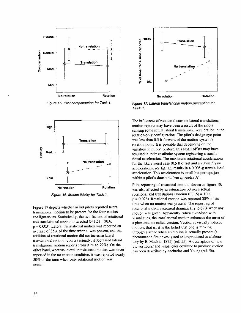
Subjective Perforrnanee Data. Figure 15 shows the

means and standard deviations of the compensation

required (i.e., extensive, considerable, moderate, or

minimum), as rated by the pilots, for the four motionconditions. When translational motion was added, the

compensation that was required significantly decreased

from considerable to moderate compensation (F(1,5) =

6.83, p = 0.047) and no significant differences were foundfor the addition of rotational motion. Rotational and

translational motion did not interact for pilot compensa-

tion. These subjective pilot opinions are consistent with

the objective control-rate differences just discussed. Thatis, the addition of translational motion reduced control

activity, which in turn likely reduced pilot opinion of the

required compensation.

Similar results were obtained for the pilots' rating of

motion fidelity, as shown in figure 16. When translational

motion was added, the motion fidelity rating improved

(F(1,5) = 7.74, p = 0.039). The fidelity increased from

low-to-medium to medium-to-high, on average. Although

the data visually suggest an improvement in fidelity with

the addition of rotational motion, the improvement was

not statistically significant. Rotational and translational

motion did not interact in the fidelity ratings.

21

Extens.

Consid.4='Mme"0D.

Eo Mod.(3

Min.

It No translation

_ ;__i I

L i@______ __Translation

"0

0O.

==

0

E

C

(D

E

"6

100%

O%

ranslstion

No translation i-

.i

t T

I

f

I


Figure 15. Pilot compensation for Task 1.


Figure 17. Lateral translational motion perception forTask 1.

010

iT.

High

Mad.

Low

Translation

T1- No translation_._

]i i


Figure 16. Motion fidelity for Task 1.

Figure 17 depicts whether or not pilots reported lateral

translational motion to be present for the four motion

configurations. Statistically, the two factors of rotational

and translational motion interacted (F(1,5) = 30.6,

p = 0.003). Lateral translational motion was reported an

average of 85% of the time when it was present, and theaddition of rotational motion did not increase lateral

translational motion reports (actually, it decreased lateral

translational motion reports from 91% to 79%). On theother hand, whereas lateral translational motion was never

reported in the no-motion condition, it was reported nearly

50% of the time when only rotational motion was

present.

The influences of rotational cues on lateral translational

motion reports may have been a result of the pilots

sensing some actual lateral translational acceleration in the

rotation-only configuration. The pilot's design eye-point

was less than 0.5 ft forward of the motion-system's

rotation point. It is possible that depending on the

variation in pilots' posture, this small offset may have

resulted in their vestibular system registering a transla-tional acceleration. The maximum rotational accelerations

for the likely worst case (0.5 ft offset and a 20°/see 2yaw

accelerations, see fig. 12) results in a 0.005-g translational

acceleration. This acceleration is small but perhaps just

within a pilot's threshold (see appendix A).

Pilot reporting of rotational motion, shown in figure 18,

was also affected by an interaction between actualrotational and translational motion (F(1,5) = 10.4,

p = 0.023). Rotational motion was reported 30% of the

time when no motion was present. The reporting of

rotational motion increased dramatically to 87% when any

motion was given. Apparently, when combined withvisual cues, the translational motion enhances the onset of

a phenomenon called vection. Vection is visually inducedmotion; that is, it is the belief that one is moving

through a scene when no motion is actually present (a

phenomenon first investigated and reproduced in a labora-

tory by E. Mach in 1875) (ref. 55). A description of howthe vestibular and visual cues combine to produce vection

has been described by Zacharias and Young (ref. 56).

22

"OO

On

£

O

E

oO

E

"6

100%

o%

Translation

T

Jti/ I

I

I /

I

I

_L

J

f

J

J

J

No translation


Figure 18. Rotational motion perception for Task 1.

To summarize the results for this task, translational

motion was clearly the most important motion variable.

Translational motion improved pilot-vehicle performance,

lowered control activity, lowered pilot compensation,

improved pilot impression of motion fidelity, and caused

pilots to believe that rotational motion was present whenit was not. The addition of rotational motion showed no

statistically significant improvement, with the exception

of a marginal statistically significant decrease in thenumber of overshoots.

Task 2:180 ° Hover Turn

Objective Performance Data. Figure 19 is a

representative time-history of several key variables for theTranslation+Rotation motion and Motionless conditions

in Task 2. Peak math model, and thus visual, yaw rates

for this turn were 50°/sec (not shown). These rates were,

of course, attenuated by the motion system (table 1) sothat it remained within its displacement constraints. In the

Motionless configuration, an increase in yaw overshoots

is noted, which is evident in the displacements, rates,

accelerations, and control inputs. These trends areconsistent with those of Task 1.

Figure 20 depicts, for the four motion conditions, themeans and standard deviations of the number of times

pilots overshot the +3 ° heading criterion about the runway

centerline during the 180 ° turns. When translationalmotion was added, the decrease in the number of over-

shoots was marginally significant statistically (F(1,4) =

5.40, p = 0.081). Interestingly, in this case, the addition

of rotational motion made the performance worse, and this

result was statistically significant (F(1,4) = 13.26,

p = 0.022). Rotational and translational motion did notinteract in this measure.

These results are not easily explained; however, it must beremembered that in this task the motion platform never

presented the pilots with full math-model motion. It is

therefore possible that some false cueing in rotation,

owing to the motion filter and its selected parameters, had

a negative effect on performance in this case. A rough

approximation confirms this possibility. For instance, if

one modeled the yaw rotation between 0° and 180 ° by

.= -- sm rot (10)

2

then the peak yaw rate would be (n/2)o_. Since the peak

yaw rates were 50°/sec, this gives a natural frequency of

approximately 0.6 rad/sec. This frequency is a reasonable

approximation of the heading time-histories, if onediscounts the holding times at both 0° and 180 °. That is,

the periods would be about ! 0 sec. Since the yaw rota-tional motion filter for this configuration had a break

frequency of 0.55 rad/sec, the motion cue's phase distor-tion at the task frequency was 90 °. It is possible that this

distortion was adversely affecting performance.

Figure 21 illustrates the rms pedal rate for this task. The

analysis of variance indicated that the decrease in pedal ratewas statistically significant when translational motion

was added (F(I,4) = 11.69, p = 0.027). No significantdifferences were noted when rotational motion was added,

and translational and rotational motion effects did not

interact.

Subjective Performance Data. The average pilot-

rated compensation required for this task is shown in

figure 22. Large variations in pilot opinion occurred, butno statistically significant differences were noted. Based on

the variation in the data, one cannot say that the motion

configurations affected the amount of subjective compen-

sation required. However, the trends shown in figure 22

follow those in Task 1 (fig. 15).

Figure 23 shows the mean motion-fidelity ratings for

Task 2. Here motion fidelity was significantly higher

when translational motion was present (F(I,4) -- 47.9,

p = 0.002), whereas the presence of rotational motion did

not affect rated fidelity. Rotational and translational effects

did not interact. So, pilots believed that the lack of trans-

lational motion was objectionable as compared to flight.

However, the lack of rotational motion, as long as there

was translational motion, was not perceived as a fidelity

degradation.

23

0

o

a

100

50

o

-50

-10o

-150

5

a n

10o

0

-50!

-100

, -150

¢MeJ

-5

¢3

-5

tn i J

5O 50

"0

o _ o

-50 -50

2 2 ....

c C

-1 -1

-2 .... -2 , ,

0 20 40 60 80 0 20 40 60 80

Time, sec Time, sec


24

10

6OOt-

.a® 4>O

'5d 2

Z

-2

T

I

I

t I

} No translation i _

Translation


Figure 20. Measured pefformance for Task 2.

High

m

Med.

Low

Translation t

T

T No translation _ _K

J_/



1.5tJI1)

e-

"lOOD.

w

Err 0.5

Extens.

r"

o Consid.

wC(llQ.

Eo Mod.

Min.

T

I T

I INo translation

i Translation .LI


Figure 21. Control rate for Task2.

T

I

/ No translation

ITranslation

±



Figure 24 illustrates pilot reports of whether lateral

translational motion was present. There were significantly

more reports of lateral translational motion when it was

present (70%), than when it was not (5%) (F(1,4) = 14.8,

p -- 0.018). There was no significant effect of rotational

motion on lateral translational motion reports, nor was

there any significant rotational motion and lateral

translational motion interaction (unlike Task 1).

In the reporting of rotational motion, the rotational and

translational motion factors interacted (fig. 25) (F(I,4) =

20.0, p = 0.011). Rotational motion was reported 90% of

the time when translational motion was present, both

when rotational motion was actually present and when it

was absent. Only when translational motion was absent

did the presence of rotational motion lead to increased

reports of rotational motion. When no motion was

presented, rotational reports occurred 27% of the time on

average, but increased to 65% of the time when a

rotational motion was added.

To summarize lhe resulls for this task, lateral translalional

motion was again the key motion variable. Its addition

reduced control activity, improved motion fidelity, and led

to the belief that rotational motion was also present when

it was not present. These results are similar to those of

Task 1, except for the interesting result that the addition

of rotational motion degraded performance slightly in

Task 2.

25

"Om1::OQ.

.o

OE

t-

O

100%

(b _Translation

)

T

- No translation

± ±



13O1:0D.

0E_JeGE

"6

100%

0%

Translation

g /

f

I .//

/

_,_ No translationI

// I

I

±



Task 3: Yaw Rotational Regulation

Objective Performance Data. Figure 26 depicts key

variables in a sample run for the Translation+Rotation and

Motionless conditions in Task 3. The peak yaw rate for

this run was 7.5°/sec (not shown). The peak yaw

accelerations for this task were similar to those of Task 1,

but the rms accelerations were slightly higher in Task 3

than in Task 1 (5.67°/sec 2versus 4.21°/sec2, respectively).The amount of visual rotation was less in this

disturbance-rejection task than in the command task of

Task 1. Slightly more acceleration overshoots were

present when motion was removed.

Figure 27 depicts, for the four motion conditions, themeans and standard deviations of the number of times

pilots had an excursion outside +1 o about north per run.When translational motion was added, the decrease in

the number of overshoots was statistically significant

(F(1,4) = 8.06, p = 0.047). The addition of rotational

motion did not yield a significant difference. The effects ofrotational and translational motion did not interact in this

measure.

Figure 28 illustrates the pedal rate for the four

configurations. Unlike the results for the previous two

tasks, the addition of translational motion did not signifi-

cantly reduce the rms pedal rate. However, the addition of

rotational motion actually increased pedal rate (F(1,4) =

18.74, p = 0.012). The rotational and translational motioneffects did not interact. So this is another case in which

the addition of rotational motion made matters worse;

however, as figure 28 shows, the percentage increase incontrol rate was not dramatic.

The cause for the performance degradation with the

addition of rotational platform motion is unknown. The

opposite result occurred in Task 1. No attempts were made

to explain why with an analytical model; that is left forfuture work. However, during the model development, a

modeler will face the difficulty of determining how a pilot

integrates both the rotational and translational cue.

Subjective Performance Data. Average pilot

compensation ratings are shown in figure 29. The

improvement in the ratings for the translational motion

conditions, relative to those in the rotational motion

conditions, was marginally significant (F(1,4) = 6.38,

p -- 0.065). The addition of rotational motion resulted in

no statistical difference in compensation. The effects ofrotational and translational motion did not interact.

The same result occurred for rated fidelity, which is

presented in figure 30. The addition of translational

motion resulted in an improvement in fidelity ratings that

was marginally significant (F(I,4) = 6.15, p = 0.068).

The addition of rotational motion again made no differ-ence. The effects of rotational and translational motion

were statistically independent.

Figure 31 illustrates the percentage of the time that pilots

reported the presence of lateral translational motion. The

addition of translational motion significantly increased the

number of reports of lateral translational motion (F(I,4) =

12.1, p = 0.025). Interestingly, the addition of rotational

motion led to a marginally significant decrease in the

reports of lateral translational motion (F(1,4) = 5.4,

p = 0.08).

Figure 32 illustrates the percentage of the time that pilots

reported the presence of rotational motion. No significant

effects were found, with rotation being reported an average

of 73% of the time, independent of the motion

configuration.

26

10 10

OIO

"O

.9

I

-5

-10

5

04(J

0

-5

O1

"O

=-O

°-

o3:e0>-

OdO

o_

2_

<

-5

-10

5

-5

I

J

Ii

Hf_

O4 2OoQ

Q

2® 0

2

_ -20

r-

w"o

a.

-2 J J

50 100 150

Time, se¢

¢D

-20 50 100

Time, sec


27

28

50

40

O

o 30

(II>0

"6 20li

Z

10

T

T INo translation

1


Figure 27. Measured pefformance for Task 3.

1.5

M"OI)Q.e 0.5E

¢C

0

I

kb

I Translation l IL

±

i i


Figure 28. Control rate for Task 3.

Extens.

I-o Conaid.IQmCOrlEo Mod.O

Min.

I No translation

I

1 Translation

T-4

±



High

._ Med.t Translation

T

i No translation

i)

T

±

Low -



"o(b1:0O.

0E

e-

<,.,oE

.i

"8

100% -

0%-

T

_ranslation

I

I

I No translation

T

)1(

i



o,oo. I' I_ T

0cL (]) I Translation

E I No translation I.,.;2 I I

IE i= j_"6

0%-



In summary, the results of this task do not reveal manydifferences from those of Tasks 1 or 2. Lateral transla-

tional motion was again the dominant variable. Its

addition improved pilot-vehicle performance, although its

effect on rated pilot compensation and fidelity was lessreliable than it was in the other two tasks. The only

statistically significant effect of rotation was a deleterious

effect on control activity.

Combined Results

Table 2 summarizes the effects of the presence of lateral

translational or yaw rotational motion on the six meas-

urables for the three tasks. All of the improvements in the

measures occur for the presence of lateral translational

motion, except for one. In that case, a marginally

significant effect was noted in pilot-vehicle stability forthe addition of yaw rotation. Statistically significant

degradations in the measures occurred only for the addition

of yaw rotational motion. Interactions between lateraltranslational and yaw rotational motion occurred only in

the lateral translational and yaw rotational motion

perception reporting. However, in Tasks 1, 2, and 3,

pilots reported (on average) rotational motion being

present 87%, 90%, and 80% of the time, respectively,

when only lateral translational motion was present.

The claim made as a result of these evaluations is that

yaw rotational platform motion is not adding value to

helicopter flight simulation. However, the claim that yaw

rotational platform motion does not provide a cue is not

made. During the course of these studies, a hypothesis

was raised that the pilots simply were not sensing

whatever cue the yaw rotational platform motion was

providing. As previously stated, each task resulted in

enough motion so that the physiological thresholds, as

measured in passive situations, were exceeded. However,

the possibility remained that, since the pilots were

actively a part of the control loop rather than passive

observers, those passive thresholds may have risen to the

point that the yaw rotational motion platform cue was not

being sensed.

This hypothesis is rejected based on the following. Todetermine if whatever cue the yaw rotational platform

motion might be providing was indeed being sensed, an

additional motion configuration was evaluated on an ad

hoc basis. That configuration simply reversed the sign in

the yaw rotational platform motion command. So for

math model rotations to the right, the visual scene

correspondingly moved to the right, but the platform

moved a symmetric amount to the left. This configuration

was extremely disliked by all the pilots, some of whom

experienced physical discomfort. Thus, what appears to be

happening in the typical motion configuration (with

correct motion signs) is that the yaw rotational platform

motion cue is simply confirming the already compellingrotational cues that come from the visual scene. This

conclusion is also supported by the earlier studies

performed by the author (refs. 48, 49) in which the pilot

was sitting at the rotational center. In that case, no

translational cue was present, so the yaw rotational cuewas redundant with the visual cue.

Table 2. Summary of yaw task results.

Measure

Translational Rotational

Task: 1 2 3 1 2 3

Translational/

rotational interaction

1 2 3

Pilot-vehicle stability + + + + - 0

Control rate + + 0 0 0 -

Compensation + 0 + 0 0 0

Fidelity + + + 0 0 0

Translational reporting + + O -

Rotational reporting 0 0

X

X X

+: Significant improvement; +: marginal improvement; -: significant degradation; O: no effect; X: interaction.

29

Inadditiontothesecompellingvisualcues,whenlateraltranslationalmotionispresent,itscombinationwiththevisualcuesprovidesmorethanenoughcuestocausethepilottobelieveheisrotatingwhenheisnotphysicallyrotating.Whentheyawrotationalplatformcueisin theoppositedirection,it isnolongerprovidingconfirmation,butit isinsteadprovidingconflict.Consistentwiththisexplanationisthedictum"badmotionisworsethannomotion"inthatspuriousmotioncuesdestroyanyvectionthathasbeengeneratedbytheothermotionandvisualcues(ref.9).

Earlierit wasstatedthatMeiry'syawexperiment(ref.22)showedthattheadditionof rotational motion improved

performance. It is possible that the difference in experi-

mental setup between that experiment and the one reported

here could account for the difference, although the results

of Task 1 in the present study did agree with those of

Meiry by showing a marginal improvement in perfor-

mance. In Meiry's experiment, pilots countered a consid-

erable yaw rotational disturbance (white noise with a15° rms), did not control a model representative of a

helicopter (the model resulted in yaw rate proportional to

pilot input at all frequencies), and the visual system was a

line on an oscilloscope. So, with this deprived-cue visual

system and with only a yaw rotational cue, yaw rotational

motion might have helped. However, Meiry's study didnot determine if the lateral translational motion cue could

have provided an equivalent substitute for the yaw

rotational cue, which was the principal result shown here.

Effect of Results

The effect of these results is twofold. First, for simulators

with independent-axis motion drives, that is, dedicated

servos for each axis, excluding the yaw platform rotational

degree-of-freedom capability would result in a cost savingsto manufacturers. To users of motion simulators that

already have a yaw rotational degree of freedom, less time,

if any, needs to be spent configuring and tuning that axis

for a given application.

Second, for simulators without independent-axis motion

drives, such as the common synergistic hexapod motion

systems (fig. 33), not using the yaw platform rotational

degree of freedom allows for more available displacementin the other motion axes. Since the same set of actuators

is used to move the platform to a desired position or

orientation, the available displacement or orientation of

any axis is a function of the displacement or orientation inanother axis.

An example of the dependency is shown in figure 34,

which was generated by Cooper and Howlett (ref. 40).

Loss of available motion in the longitudinal, lateral, and

vertical axes also occurs for rotations about the yaw axis.

Thus, users should disable yaw rotation and thereby gain

additional benefits in axes that provide added value in

flight simulation.

Figure 33. Typical hexapod motion drive system.

6O

4}"0

d"0= 0.H_II

0n.

-6O-60 0 60

Pitch attitude, deg

Figure 34. Effect of yaw angle orientation on pitch and roll

angles.

30

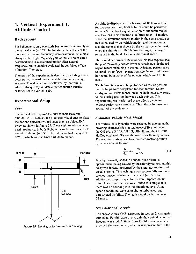
4. Vertical Experiment I:

Altitude Control

Background

For helicopters, only one study has focused extensively onthe vertical axis (ref. 24). In that study, the effects of the

motion-filter natural frequency were examined, but almost

always with a high-frequency gain of unity. The researchdescribed here also examined motion-filter natural

frequency, but in addition evaluated the combined effects

of motion-filter gain.

The setup of the experiment is described, including a task

description, the math model, and the simulator cueing

systems. This description is followed by the results,

which subsequently validate a revised motion-fidelitycriterion for the vertical axis.

Experimental Setup

Task

The vertical task required the pilot to increase aircraft

altitude 10 ft. To do so, the pilot used visual cues to place

the horizon between two red squares on an object 50 ft

away, as shown in figure 35. These sighting objects were

used previously, in both flight and simulation, for vehiclemodel validation (ref. 57). The red region had a height of

0.75 ft, which was the final altitude tolerance.

/0.75 ft _ Horizon

i"l'i2.! ft 10 ft

Red

111-Figure 35. Sighting object for vertical tracking.

An altitude displacement, or bob-up, of 10 fl was chosenfor two reasons. First, 10-ft bob-ups could be performed

in the VMS without any attenuation of the math modelaccelerations. This situation is referred to as l : l motion,

since the simulator cockpit motion is the same motion as

that calculated by the vehicle model, and the motion is

also the same as that shown by the visual scene. Second,when the aircraft was 10 ft below the target, the target

remained in the field of view of the visual scene.

The desired performance standard for this task required that

the pilot make only two or fewer reversals outside the red

region before stabilizing in the red. Adequate performance

required two or fewer reversals outside the top and bottom

horizontal boundaries of the objects, which are 2.25 ft

apart.

The bob-up task was to be performed as fast as possible.

Five bob-ups were completed for each motion-system

configuration. Pilots repositioned the helicopter downward

to the starling position between each bob-up. This

repositioning was performed at the pilot's discretion

without performance standards. Thus, the bob-down was

not part of the evaluation.


The vertical-axis dynamics were selected by averaging the

hovering characteristics (at sea level) of five helicopters:the OH-6A, BO-105, AH-1G, UH-1H, and the CH-53D.

Heffley et al. (ref. 58) was the source for these dynamics.

The resulting vertical-acceleration-to-collective-position

dynamics were as follows:

il 9s

_-(s)- (ll)s+0.3

A delay is usually added to a model such as this to

approximate the lag caused by the rotor dynamics, but this

delay was instead subsumed by the simulator motion and

visual systems. This technique was successfully used in a

previous model validation experiment (ref. 59). Inaddition, no torque or rpm limits were imposed on the

pilot. Also, since the task was limited to a single axis,there was no coupling into the directional axis. Atmo-

spheric conditions were calm air, no turbulence, andunrestricted visibility. The math model cycle time was25 msec.


The NASA Ames VMS, described in section 2, was again

employed. For this experiment, only the vertical degree of

freedom was used. A Singer Link DIG-I image generator

provided the visual scene, which was representative of thc

31

stateoftheartinthelate1970s.Thisvisualimagegeneratorwasdifferentfromthatreportedinsection3,aresultofschedulingconstraintsattheVMSfacility.Theimagegeneratorthatwasuseddidnothaveatexturingcapability.Thevisualdelayfromthemathmodeltothevisualimagewas83msec(ref.52),whichisatypicaldelayforflightsimulatorimagesystems.Visualleadcompensationwasnotusedtoreducethevisualdelay,thepurposebeingtomorecloselymatchthevisualandmotiondelays.Thismatchingisimperfect,sincethevertical-axisfrequencyresponsecanbeapproximatedbyanequivalenttimedelayof 140msec(eq.(4)).Thus,inthisexperiment,thevisualresponseeffectivelyleadsthemotionresponse.Thevisualfieldofviewwaspresentedonthreewindowsthatspanned+78 ° horizontally and +12 ° and-17 ° verti-

cally as shown in figure 36. The center window had the

principal objects in the field of view for the task, and the

information presented in the left and right windows was

limited to polygonal color variations on the ground. The

image that the pilot viewed for the task is shown in

figure 37.

t t t I r_

#,-,---'v--7_; -_ --/--4--,_'-- /

'_:75z:-:_-<_-.._ _k.,z/;._.:.;._>--:-->_-

Figure 36. Cockpit field of view for vertical tracking.

A conventional left-hand collective lever was used. It had a

travel of +_5in, had no force gradient, and the friction was

adjustable by the pilot. All flight instruments weredisabled so that all cues were from the visual scene and the

motion system. Rotor and transmission noises werepresent to partially mask the motion-system noise. The

head-up display shown in figure 37 was stowed for the

task. Three NASA Ames test pilots participated; they arehereinafter referred to as pilots A, B, and C. All three fly

rotorcraft and had extensive simulation experience.


A second-order high-pass filter, typical of that used in

most flight simulators, was placed between the mathmodel vertical acceleration and the simulator-commanded

acceleration. It had the form of

Ks 2

ilc°m (s)= s2 (12)+ 2_toS + to2

where hcom is the commanded vertical acceleration of the

simulator cab, h is the math model's vertical acceleration

at the pilot's station, K is the motion gain, _ is the

damping ratio, and to is the filter's natural frequency.

The damping ratio of the above filter was held fixed at

0.7. The two parameters that are used to then keep the

motion system within its displacement limits for a givenmath model and task are K and to. To reduce simulator

motions, either K is reduced or to is increased. Achieving

the proper balance between these two possible ways of

reducing the motion, while trying to minimize a loss

in motion fidelity, is not well defined. The criterion

suggested by Sinacori and discussed in section 1 was usedto select the characteristics of the motion configurations.

To validate or modify the criterion, 10 sets of gains and

natural frequencies were chosen to span the criterion, as

shown in figure 38. The values for the filter are given in

table 3. Note that configurations V3 and V4, fromtable 3, result in gain and phase-distortion coordinates of

[0.970, 45.01 and [0.795, 80.0[, respectively. Although

these filters have unity gain at high frequencies (K = 1),

the dynamics of the high-pass filter cause the abovc

attenuations and phase distortions at 1 rad/sec, which isthe frequency used to plot the motion filters against thecriterion.

Figure 37. Pilot's visual scene for vertical tracking.

32

\Fixed base

(u = 0.885 rad/sec

(x)= 0.521 rad/sec

(;) = 0.245 rad/sec

Low

I I0.0 0.2

I I0.4 0.6

Gain @ 1 rad/sec

Medium

High

0.8

Figure 38. Motion configurations for vertical tracking.

8O

60

40

20

0

1.0

O_(D

"lD

T-

@

J:

Table 3. Motion-filter quantities for vertical tracking.

Vertical

Configuration K co

(rad/sec)

V1 1.000 0.010

V2 0.901 0.245

V3 1.000 0.521

V4 1.000 0.885

V5 0.650 0.245

V6 0.670 0.521

V7 0.300 0.245

V8 0.309 0.521

V9 0.377 0.885

V 10 0.000 --

Procedure

For the pilot to rate the motion fidelity of each

configuration, a baseline was established for comparison.

The baseline specified that the pilots perform the task first

with 1:1 motion; this was a calibration run. Here, the

pilots were told that they had 1: 1 motion, and that the

sensations they were feeling were to be interpreted as the

"actual aircraft." The motion fidelity of all future config-

urations was then compared to this 1 : 1 motion baseline

configuration. This testing procedure allowed immediate

back-to-back comparisons of the effects of motion

parameter changes. This procedure mitigates some of the

problems that occur in simulation fidelity experiments

that compare the actual aircraft to the simulation back-to-

back, even when the events occur in the same day.

33

During the evaluations, the pilots had no knowledge of

the configuration changes, except when they were told ofthe full-motion "calibration runs." Still, the 1:1 motion

case (configuration V1 in table 3) was also evaluated;

during its evaluation, the pilot was not told he had the

1: 1 configuration.

Pilots A and C completed all the configurations listed in

table 3 in one session, Pilot B completed all the config-

urations in two sessions, and all of the configurations

were evaluated by all three pilots. Some configurations

were repeated if time permitted. For each configuration,

pilots assigned a motion-fidelity rating using the defini-

tions in figure 4. Then, the pilots answered questions

regarding the aircraft's characteristics, their task perfor-

mance, and the compensation required to perform the task.

The pilots were also asked to estimate the relative use ofthe motion and visual feedback cues.

Results

The results of Vertical Experiment I consist of objective

performance data and subjective fidelity ratings. Relevant

pilot comments will be added in the discussion of theseresults.

Objective Performance Data

Again, compelling performance differences are shown

between full motion and no motion in figure 39

(configurations V1 and V 10, respectively). For the

configuration VI case, well damped, accurate bob-ups

were achieved with the vertical velocity remaining within

10 ft/sec; the vertical acceleration remained within 0.5 g,

and the collective stayed within 1.5 in. A drastic difference

is evident in the no-motion case (V10). Initially, the pilotovershot the 85-ft desired altitude and then returned to the

starting point as he responded to the unfamiliar cues.

Since the acceleration feedback cue was the only cue that

changed from the full- to the no-motion case, part of the

pilot's collective input must have been a result of thatcue. With the acceleration cue removed in the V10

configuration, the pilot had to adjust his compensationbased on the new set of cues. With time in the motionless

configuration, the performance improved, but even the

final repositioning took longer in the fixed-base case thanin the full-motion case. These differences have obvious

training implications, for the pilot must develop different

mental compensation between the two cases. No data were

taken when returning to the full-motion case for recalibra-

tion, but pilots commented that relearning the full-motion

configuration was easy and natural.

Figures 40 through 49 show phase-plane portraits for each

motion configuration. Each portrait shows three runs, one

for each pilot, using his best performance run if an evalu-

ation was repeated. Both the bob-up and bob-down arc

shown. These plots show how the motion changes

affected the pilot's ability to capture the upper desired

point smoothly. Ideally, these plots should be well-

damped and approximately oval.

Figure 40 indicates that some overshoots were present for

the full-motion condition, but overall the trajectories were

well damped and smooth. There was reasonably precise

control about the 85-ft altitude point, with one instance of

a pilot not arresting the vertical velocity soon enough,

which caused a position overshoot. Little change in

performance, or perhaps a slight improvement, is noted

for the slight motion changes of configuration V2 in

figure 41.

The high-gain, moderate phase-distortion case of

configuration V3 in figure 42 still produces well-damped

trajectories on ascents. The acceleration cues for this

configuration lead the math model by 90 ° at 0.52 rad/sec.If the motion between the ascents and descents were sinu-

soidal, the frequency of the maneuver would be approxi-

mately 2 rad/sec. This value is approximated by letting

h = 80 + 5sin cot (13)

1_= 5oJcoso_t (14)

max = 10 ft / sec _ co = 2 rad / sec (15)

For the initial phase of the maneuver, therefore, the

motion cues would be accurate, but the subsequent

stabilization at a particular altitude would produce some

miscues, for lower frequency content would be present.

Pilots seemed to have more difficulty in returning to the

starting point than in the first two configurations;

however, this repositioning was not officially part of the

evaluations. For the high-gain and high-phase-distortion

case of configuration V4 in figure 43, the overshoots were

more prominent, and the overall control was much less

precise.

34

90 90

85

75

70

85

_= so

75

7O

10

5

0>

d-5

>

-10

-15

10

5

_." 0

>

>

-10

-15

20

U

® 10

c 0¢,}

_ -lO0

>

-2O

-30

2O

10

= 0

_ -lO0>

-20

, , -30

2

-2

-3

50 100 0

Time, sec

50

Time, sec

100

Figure 39. Altitude control: full motion versus no motion.

35

36

90

85

75

7O-20 -10 0 10 20

Vertical velocity, ft/sec

Figure 40. Phase-plane portrait for configuration Vl.

90

85

d==8o

75

I

: • :._i:_i I_:.iI

\ /

\70

-20 -10 0 I 0 20

Vertical velocity, f',Jsec

Figure 4 I. Phase plane portrait for configuration V2.

90

85

=_=80

751\

\

\\" ,-"/i70

-20 -10 0 10 20

Vertical velocity, ftJsec

Figure 42. Phase-plane portrait for configuration V3.

90

I .

85

d

75 _ :

\

7O-20 -10 0 10 20

Vertical velocity, ft/$ec


For the medium-gain, low-phase-distortion case of

configuration V5 in figure 44, the bob-up trajectoriesshow good performance, with the trajectories being

similar to those of the full-motion case, or at least similar

to those of the V2 case. The gain is lowered to 65% of

full motion for the V5 configuration.

Increasing the phase distonion from configuration V5 to

configuration V6 caused a slight reduction in the precision

around the desired stationkeeping point with a few under-

shoots of the ascent point as shown in figure 45. The gain

reduction in going from V3 to V6 does not appear to

degrade performance significantly.

The low-gain, low-phase-distortion case, configuration V7

in figure 46, resulted in less precision with more over- and

undershoots than in the previous configurations. Here the

gain is at 30% of full motion at high frequencies.

Performance definitely decreases when the gain drops from

0.65 in configuration V5 to 0.3 in V7.

The precision in V7 also appears worse than in the V4

case of high gain and high phase distortion. Increasing the

phase distortion to the V8 case in figure 47 shows a

further reduction in precision from that of the V7 case.

Again, the gain of 30% is insufficient, but the combina-

tion of the low gain with some phase distortion makes the

performance even more degraded.

The low-gain, high-washout case of configuration V9 in

figure 48 exhibits a further degradation, the middle of the

desired oval being occupied with the aircraft's trajectory.

Finally, the no-motion case of configuration VI0 in

figure 49 indicates the worst performance of all; the

imprecise control of velocity is obvious at both the top

and bottom points.

90

85

4::

so

,<

75

70

iI.

\_ /

-20 -10 0 10 20

Vertical velocity, ft/se¢


90

85

d"0

,.._=8o.,,,,,,

<

75

7O-20 -10 0 10 20



90

85

4::c-

so

75

7O

w

•...j i¸ -

\ K-2(\\ \ j J

-20 -10 0 10 20



90

85

"_ eo

75

\ I70 _' '

-20 -10 0 10 20

Vertical velocity, flJsec


90

85

d

,,,..,

75

:: y i¸

\\ (-- ,_/

\,_1 /70

-20 -10 0 10 20



90

85

¢:d

eo

<

75

'lll:_x --_. _\ _tI

\

J

70-20 -10 0 10 20


Figure 49. Phase-plane portrait for configuration V l O.

3?

Subjective Performance Data

Figure 50 shows pilot motion-fidelity ratings along with

the postulated boundaries of Sinacori (ref. 44). The pilots

unanimously rated the high-gain, low-washout configura-

tions V 1 and V2 as having high fidelity. If either the gain

was reduced (as in V5) or the phase distortion increased

(as in V3), one of the three pilots reduced his rating to

medium. When a combination of this gain and phase

distortion was examined, that is, configuration V6, the

ratings dropped on average across one level. However, one

of the pilots did not perceive differences between the V3 or

V5 configuration and the V6 combination.

@Vl0Fixed base

Low

_ - Pilot A

] - Pilot B

O - Pilot C

[]®

.100

8O

6O

I I I0.0 0.2

Medium

2O

tl

®o0.4 0.6 0.8 1.0

Gain @ 1 rad/sec

Figure 50. Motion fidefity ratings for altitude control.

A

4)

@

i@

U.Ca.

The next individual changes in gain or phase from the V3

and V5 cases to the V4 and V7 cases produced, on average,

a decrease from high to medium fidelity. However, acombination of these effects, encompassed by the V9

configuration, produced unanimously low fidelity ratings.

Unsurprisingly, the fixed-base configuration, V 10, also

produced unanimously low fidelity ratings.

These ratings suggest that for this task, the fidelity

criterion for the vertical axis appears to decrease from

high-gain/low-phase-distortion in a direction toward the

fixed-base case. The combination configurations V2,

V6, and V9 result in ratings predicted by the criterion.

However, either reducing the gain or increasing the phase

distortion resulted in fidelity ratings better than predicted,

on average.

Combined Results

It is reasonable to suggest a revision to the Sinacori

criterion (ref. 44) if objective performance, subjective

pilot fidelity ratings, and subjective pilot comments are

consistent. Each of the configurations is discussed, and

when a consistency exists that does not align with the

criterion, then a modification to the criterion is suggested.

With the full-motion case, configuration V l, pilots were

consistent in their comments that they achieved desired

performance, that compensation was minimal to moderate,

and that they felt that they could be very aggressive with

the vehicle. All ratings were high fidelity, and the

objective performance was good.

For the configuration with a slight decrease in gain and an

increase in phase distortion, V2, the comments indicated

that a difference was noted. Two of the three pilots noticed

a slight decrease in performance, and the compensation

increased over that of the V 1 case. Yet all pilots rated the

configuration high fidelity, since they felt is was "close to

visual flight." Here is where the fidelity definitions could

be made more precise, because a pilot is faced with a

potential dilemma with a configuration that has noticeable

but not objectionable differences (medium fidelity defini-

tion), yet is close to visual flight (high fidelity defini-

tion). Pilots apparently felt that when it was necessary to

group the ratings into three categories, the V2 configura-

tion was in the most favorable category. Yet they all

perceived a difference. It appears that the pilots may havebeen sensitive to the differences in the immediate accel-

eration because of collective input. This initial accelera-

tion is proportional to the high-frequency motion gain,

and it is reasonable that the 10% change between these

configurations could be noticed. It is also reasonable that

the variation was not objectionable.

For the high-gain and moderate phase-distortion case,

configuration V3, all pilots noticed the necessity to

change their control input technique. Two pilots noticed

the unpredictability, or the "slipperiness," of this config-

uration. Only one downgraded the fidelity rating to

medium. The objective performance did not change

appreciably in the bob-up, but difficulty was perceived in

repositioning downward. Although the ratings indicated

the configuration was high fidelity, the comments and the

performance did not agree. Thus, the V3 configuration

should not be placed in the high-fidelity region.

Increasing the phase distortion further to the V4

configuration resulted in a perceived degradation in

38

performance,andthisisevidentfromthephase-planedata.Theaggressivenesslevelwasreduced,andtherequiredcompensationincreased.Twoofthethreepilotsnoticedaphasingdifferencebetweenthevisualandthemotioncues,yetwithalloftheabove,theyratedthisconfigurationnoworsethanmedium.However,onepilotthoughtthatitwasclosetobeingobjectionable.Consideringthecommentsandtheperformance,it appearsthatthefidelitywasclosertolowthantheratedmedium,andthusnochangeissuggested.

Comparingthesenear-unitymotiongainresultswiththeonlyothersetofhighqualityexperimentaldataforheli-copters(ref.24)showssimilartrends.Thatexperimentshowedthatfortrackingarandomlymovingtarget,whiletheopen-loopcrossoverfrequencyremainednearlyinvariantwithincreasesinmotion-systemphasedistortion,thephasemarginincreasedby30° whengoingfromamotionphasedistortionof 108° toaphasedistor-tion of 16°. For a phase distortion of 43 °, which is similar

to configuration V3, a phase margin degradation of 15°

was measured. The comments and objective performance

data from the present experiment, for these cases, indicated

a similar trend in stability degradation, yet the subjective

fidelity ratings for this task still rated the V4

configuration as medium fidelity.

In another experiment (ref. 60), for aircraft with poor

longitudinal flying qualities in a landing task, it was

observed that phase distortions higher than 90 ° caused

"essentially uncontrolled touchdowns." Thus, considering

previous data and the lack of consistency in this experi-

ment's objective and subjective results for these config-

urations, it seems appropriate to retain the hypothesized

fidelity breakpoints suggested by Sinacori (ref. 44) for the

near-unity gain configurations.

Returning to the low phase-distortion configuration with

moderate gain, V5, pilot comments and objective perfor-

mance generally indicated no degradation from the full-

motion case. Only one pilot rated the fidelity as medium

(owing to a slight vertical oscillation). From the consis-tency of these results, it appears that when the phase

distortion is less than 30% lowering of the gain required

for high motion fidelity from 0.8 to 0.6 is appropriate.

Keeping essentially the same motion gain, but increasingthe phase distortion to configuration V6 resulted in

comments indicating a performance loss because of a

reduction in precision and aggressiveness. Fidelity ratings

of medium are consistent wJth Sinacori's hypothesized

boundaries fief. 44).

A reduction of gain to 0.3, but with a low phase

distortion in configuration V7 resulted in adequate

performance, fears of overshooting, and comments that the

motion was almost unusable. These comments were

repeated for the remaining configurations, V8 and V9; the

objective performance worsened as the phase distortion

increased. From the comments and ratings, configurationsV7, V8, and V9 were consistent with Sinacori's hypothe-

sized boundaries (re/'. 44). Therefore, regardless of the

phase distortion, a gain of 0.3 results in low fidelity.

Referring to the fixed-base configuration, VI0, two pilots

said that they put the control input in the wrong direction

during the run. Pilots were generally stunned at the effects

of the total loss of motion. During the 1:1 calibration

runs, one pilot made a comment prior to the evaluations

that "The visual scene is so compelling at conveying the

error that it seems to primarily be a visual task... I

would expect the effects of motion to be minor." Another

pilot commented after the fixed-base configuration "I have

never experienced such a dramatic disconnect from reality

as during that configuration, as compared to the full-motion case." Thus, caution should be used when inter-

preting a priori conjectures on the value of motion, even

when given by experienced test pilots with considerable

simulation experience.

Motion cues were certainly perceived by the pilots in all

but this fixed-based configuration. This is evident from

the performance and comments, but it is also consistentwith tests that have determined the vertical-acceleration

sensing threshold to be in the 0.09-0.27 ft/sec 2 range

(ref. 19). This threshold was exceeded in all but the fixed-

base configuration.

Suggested Revision to Fidelity Criteria

Based on these results, a revision to the vertical axis of

Sinacori's criterion is suggested in figure 51. Here, the

changes consist of lowering the gain required when the

phase distortion is low. The gain for the high-fidelity

region is reduced to account for the results of the V5

configuration. The medium-fidelity region has been

extended to a lower gain, but kept above that of the V7

configuration, which has a gain of 0.3. These suggestionsare consistent in trend with the data of Mitchell and Hart

(ref. 47), which indicated a preference for low-gain, low

phase-distortion motion over high-gain, high phase-

distortion motion. Also, the fidelity boundaries have been

rounded to account for the reduction in fidelity when a

gain attenuation is combined with phase distortion. The

determination of exactly where the rounding should beginand end requires additional dam.

Also, slight wording changes are suggested to the motion-

fidelity definitions of figure 4 to alleviate the previouslymentioned difficulties in their use. The word "disorienta-

tion" should be removed; it caused some pilots to shy

39

awayfromthelowrating.Althoughaconfigurationmayhavebeenobjectionable,thepilotsfeltnodisorientation.Thesuggestedrewording,asnotedonfigure51,shouldsuffice,sinceanydisorientationexperiencedwouldbeexpectedtoreceivean"objectionable"description.

Significantdifferencesinmeasuredperformanceandinperceivedfidelitywereevidentacrosstheseconfigurations.TheanalyticalmodeldiscussedinappendixBpredicteda

performancedecreasewhenthemotionfilternaturalfrequencyincreased.However,thepredictedbandwidthsoftheprimaryloopdidnotdifferbyafactorof 1.5,whichwasthegeneralguidelinesuggestedfordeterminingdissimilaritybetweenmotionconfigurationresponses(ref.61).Althoughthisanalyticalmodelisperhapsthemostreasonableavailable,thisexperimentdemonstratedthatadditionaldataareneededinordertocontinueitsrefinementandvalidation.

Vertical axis - 80

-- Ref. 44

Modified

I I0.0 0.2

Low

II/ Medium

1 l

0.4 0.6 0.8Gain @ 1 red/sec

- 6O

-40

- 20

0.0

O

{.1O

Ev-

Oe-o

o

.B"o

ool¢Br-

9.

HighMedium

Low

Motion sensations are not noticeably different from those of visual flight

Motion sensation differences are noticeable but not objectionable

Motion sensation differences are noticeable and objectionable

Figure 51. Suggested vertical criterion and fidelity definitions.

4O

5. Vertical Experiment II:

Compensatory Tracking

Background

In Vertical Experiment I, the global performance effects of

motion-filter gain and natural frequency variations were

examined during tracking. In Vertical Experiment II, amore detailed examination of the same filter variations

was conducted for a new task: key pilot-vehicle frequency-

response metrics were measured during combined trackingand disturbance regulation. This procedure allowed for the

influence of the motion-filter changes to be examined

simultaneously for these two important piloting tasks.

The task and experimental apparatus are first described.

Then, objective pilot-vehicle performance metrics and

subjective motion-fidelity ratings arc discussed.

Experimental Setup

Task

Figure 52 shows the display presented to the pilot. The

object was to null the error between the moving targetaircraft and the horizontal dashed line that was fixed to the

pilot' s aircraft.

A system block diagram depicting how the error developed

is shown in figure 53. Two external inputs were used in a

scheme similar to that developed by Stapleford et at.

(ref. 26).

Target Aircraft

Fixed horizontal lines

Figure 52. Pilot's display for vertical compensatory

tracking.

ih +

(_Cd Aircraft

l Visual ]hardware _

h

Figure 53. Vertical compensatory loop.

The target was driven by a sum-of-sines (SOS) input, andthe vehicle was disturbed by a separate SOS input that

was summed with the pilot's collective position. These

SOS's were as follows:

ih (t) = 2.573 sin(0.15t) + 2.202 sin(0.34t)

+ 1.563 sin(0.64t) + 0.923 sin(l.13t)(16)

+ 0.411 sin(2.05t) + 0.150 sin(3.56t)

+ 0.040 sin(6.32t) feet

5cd (t) = 0.029 sin(O.28t) + 0.058 sin(O.49t)

+ 0.999 sin(O.8Ot) + O.167 sin(1.50t)(17)

+ 0.209 sin(2.67t) + 0.201 sin(4.63t)

+ 0.148 sin(8.50t) inches of collective

Each component of each SOS completed an integral

number of cycles in the task time-length of 204.8 sec.

A warm-up period of 10 sec preceded the run, and a cool-

down period of 3 sec followed the run. To prevent the

pilot from separating target motion from disturbancemotion, the disturbance input, _5c_,was selected so that its

resulting altitude spectral content (when filtered by the

vehicle dynamics) matched the target shaping function(refs. 26, 41). If the pilot is able to separate the target

motion (which is sensed only visually) from the distur-

bance motion (which is sensed visually and vestibularly),

previous research has shown that pilots may alter theirbehavior and potentially ignore the motion cues when

nulling the target motion (ref. 26). The above spectral

matching is an attempt to prevent this behavior.

The above shaping function was determined empirically.

The compromised result of this shaping was that the

highest frequency component of the target input wasbelow the simulator's visible threshold of 3-4 arc min,

and the lowest component of the disturbance input wasbelow the vestibular translational acceleration detection

threshold of 0.01 g's (ref. 28). As shown in figure 53,

the pilot received two external cues for use in zeroing the

target error, e: a visual cue, and a motion cue. The

dynamics between the pilot input and these cues arediscussed in the sections that follow; however, only thc

block labeled "motion filter" was modified in this experi-

ment. The details of these blocks will be described later.

Although the pilot was instructed to null the displayed

error constantly, the desired performance for thc task was

to keep the error within one-half the height of the targetvertical tail for half of the run length. The target was

placed 100 ft in front of the aircraft, and the hcight of thcvertical tail was 3 ft.

41


The vertical-axis dynamics were the same as for Vertical

Experiment I given by equation (11). Again, only this

single degree of freedom was modeled, and the pilot

controlled this degree of freedom with a collective lever in

the cockpit.

motion fidelity of each configuration, using the motion-

fidelity definitions given in figure 4. Between each

configuration, in order to calibrate or recalibrate them-

selves to the true vehicle model response, pilots flew the

model with full motion (configuration VI) in a visual

scene depicting objects of known size (shown in fig. 35).

All six pilots flew all 10 configurations.


The simulator and cockpit were also the same as for

Vertical Experiment I. All flight instruments were again

disabled. Six NASA Ames test pilots participated (three of

the six being the same three who participated in Vertical

Experiment I), hereinafter referred to as pilots A-F. All

pilots had extensive rotorcraft flight and simulation

experience.


The second-order high-pass motion filter given by

equation (12) was used. The gains, damping ratio, and

natural frequencies evaluated were the same as for Vertical

Experiment I, which are given in table 3.

Procedure

All configurations were tested in blind evaluations, and

they were randomized. Pilots were asked to rate the

Results


Time-histories and standard deviations of several pertinentvariables for a full-motion case (V 1) and a no-motion case

(V10) are shown in figure 54. Both of these runs were

made by the same pilot. This comparison reveals that

when going from full motion to no motion, the target

error, vehicle acceleration, and collective displacement all

increase. Rather than compare time-histories across the

10 cases and six pilots, several pilot-vehicle performance

metrics were determined, and the statistical significancewas evaluated.

First, since the two sum-of-sines inputs were statistically

independent, two effective open-loop pilot-vehicle

describing functions may be determined (ref. 41 ). One

open-loop describing function applies to the target errors

caused by target motion; it is determined by calculating

the ratios of the Fourier coefficients of h(j(0)/e(j(o) at the

V1 VIO

.1= 10 __d 0

.lO r I 1 I S

2010 offi31 ft

.d

¢q o ffi7.2 ft/Nc 2

20 "_ I dll_lCl[IkJJ¢l [ =1"jlj4111'l_ljt ' JId "tllla_Ld d

:" "_ F _ 1 1 l

.,,ll t.al,0-.ab-J, Nd l. tlm|-= ,,,li" a'T T-IT' 3

2 { ] [ '] I

0 50 100 150 200

Time, sec

_L_

0 50 100 150 200

Time. 8ec

Figure 54. Compensatory tracking: full motion versus no motion.

42

target input frequencies. The other describing function

applies to target errors caused by the disturbance input; itis determined from the ratios of the Fourier coefficients of

--8_(jto)/5cLo_(Jto) at the disturbance input frequencies.

These two describing functions are referred to the "target

following" and "disturbance rejection" describing functionshereinafter.

From these describing functions, open-loop crossover

frequencies and phase margins were determined by linear

interpolation. Figure 55 shows the magnitude and phase

responses of the disturbance-rejection describing function.The data for this example are from the full-motion run

(V I ) in figure 54. Linear interpolation between the data at

the appropriate frequencies (shown in fig. 55) gives a

crossover frequency of 3.3 rad/sec and a phase marginof 28 °.

The above two measures provide useful information about

the character of the pilot-vehicle response. In particular,

the crossover frequency is a rough measure of how fast

the error is initially zeroed; the higher the crossover

frequency, the faster the initial nulling of the error. The

phase margin is a rough measure of the damping ratio ofthe error response; the higher the phase margin, the more

damped the error response.

Each of these open-loop describing functions includes a

different combination of both the pilot's internal visual

and motion compensation applied to the visual error and

to the acceleration feedback (refs. 26, 41 ). Although only

the motion cues were changed here, the pilot's internal

compensation may change in an attempt to account for

degradations in either the visual or motion cues. Theoverall effect of these changes on pilot-vehicle

performance and opinion are given next.

Target Following. The target-following crossover

frequencies are given in figure 56 for all of the config-

urations. For easy reference, the motion-filter gain K and

natural frequency to, rounded to one decimal place, areindicated above each bar. The mean value (bar height) and

standard deviation (horizontal line above bar) are shown,

each determined from six values. Each of the six values

corresponds to the individual average for each pilot across

his runs. Upon examining the variance ratio, or F-test

20

10

tn"O

a;

gg

-10

-2O

-1 O0

-150

1D

-200

a.

-250

10 "1

XX × '

-300

10 -1

L L i , L J

X

I

10 0

Crossover frequency

I :

:1

I,I

1

1

)<

I

Phase margin

X

X

, i i J I

10 0

Frequency, rad/sec

i

101

101

Figure 55. Example disturbance-rejection describing function.

43

O6

I,,.

Cm

C

EP

O"

0

£u

1.0 0.3 0.4 0.0K 1.0 0.9 0.5 0.9 0.0

CO -]-O'O 7- -1- T

O i i l A i

V1 V4 V8 V9 VIO

0.90.2 1.0

0.5

-[-

I t

V2 V3

0.3

0.7 0.7 0.20.2 0.5 7-

T T

i i i

V5 V6 V7

Configuration

Figure 56. Target-following pilot-vehicle open-loop crossover frequencies.

(ref. 54), for these data, the differences among the config-

urations were not significant at the 5% level. In addition,

no coherent trend was present among the motion-filter

variations. This result agrees with, and extends, the results

of Bray (ref. 24), which indicated an invariance in target-

following open-loop crossover frequency for motion filter

natural frequencies between 0.2 and 1.25 rad/sec with K =

1 for all configurations. The results from the present

experiment indicate that this invariance across natural

frequency variations also holds for motion-gain changes.

Thus, it appears that the initial quickness with which the

pilot closes the target-tracking loop does not depend on

the motion cue. That result is intuitive; it might be

expected that the speed with which this loop is closed

would be based on a pilot's mental model of the speed

with which the loop should be closed. The pilot initiates

and generates his own motion in this loop.

Figure 57 shows the target-following loop phase margins

for all configurations. Unlike the target-following cross-

over results, statistical differences are present in the phase

margins, although the range of the means is only l 0 °. The

largest phase margin occurred with the full-motion

condition (V1), and phase margin was progressively lost

as K was reduced and o.}m was increased. Using the

Newman-Keuls method (ref. 62) to determine which

means are statistically different from each other at the 5%

level, the results indicate that configurations V1 and V3

were different from V4 and from V6-V10, and that

configurations V2 and V5 were different from V8.

50 , _ ,

o_G)"o

40E"Or-

e_ 30Ill

E

.c 20

E

_ 10

a.

K 1.0 1.0Co 0.0 0,9 0.5 0.7

-I- 0"2-I- 1.0 0.2

-[- ._L_ 0.9 _ 0.7 0.3 0.4 O.Oo.o

i I__ 0.5 0.9

i I

I '

i

I

I i I ' t , I , , L ,

V1 V2 V3 V4 V5 V6 V7 V8 V9 Vl 0

Configuration

Figure 57. Target-following pilot-vehicle open-loop phase margins.

44

These results are partially consistent with those of Bray

(ref. 24), which indicated that target-tracking phase margin

degraded as tomwas increased from 0.2 to 1.25 rad/sec at a

unity gain (K = 1). However, Bray's results exhibited

larger variations in the measured phase margins, including

an almost 20 ° variation between tom = 0.2 and 0.5 rad/sec.

Only a slight difference was measured in this experiment

between the nearly equivalent VI and V2 motion

configurations.

These phase-margin target-following results suggest that

the resulting damping of the error to a nulled steady-statevalue is affected by motion variations. This result isconsistent with the results in section 4. That is, as the

quality of the motion improved in that purely target-

following task; the principal effect on performance was in

damping (see figs. 40--49).

It was also suggested in section 4 that the high-fidelity

portion of the Sinacori criterion should include config-

uration V5. The performance results shown here for target

following are consistent with that suggestion.

Disturbance Rejection. Pilot-vehicle open-loop

crossover frequencies for the disturbance-rejection loop are

shown in figure 58. The crossover magnitudes appear to

be roughly ordered by phase distortion level, that is, bysuccessive increases in tom.The statistical results reveal

that at the 5% level, configurations VI, V2, and V7 all

had higher crossover frequencies than the fixed-base case

V10. Again, these results are consistent with the

configurations tested by Bray (ref. 24), and they extend

those results by suggesting that the open-loop crossover

appears to be affected by changes in tomat all levels of

motion-filter steady-state gain K.

Figure 59 shows the disturbance-rejection loop phase

margins. Here the configurations are ordered by progres-

sive reductions in K. Statistically, configuration V3 was

better than any of the other cases, and configurations VI

and V4 were better than V 10. Bray showed, for K = l, that

the low and high phase distortion cases have roughly the

same phase margin, with perhaps a slight peaking at

moderate amounts of phase distortion. Here, more relative

peaking in phase margin was observed for the V3 casethan was found by Bray. The crossover frequency for

V3 was reduced, which alone might contribute to an

increased phase margin; however, V4 had a low crossover

frequency, but not an accompanying phase-margin peak.With the unknown details of the pilot feedbacks, the V3

configuration must be coupling in with the vehicle

dynamics in a manner different from that in the other

configurations.

The overall disturbance-rejection results suggest three

points. First, the speed at which the disturbance is rejected

is affected primarily by the high-pass motion filter's

natural frequency. Second, motion-filter gain appears to

affect the relative damping of the disturbance-rejection

loop, rather than being driven more by filter natural

frequency as in the target-following loop. Third, both the

lowest crossover frequency and the lowest phase margin of

the disturbance-rejection loop occurred in the no-motion

case.

4 i 1'.0o i K

Q_w 03

t-

p.

_2-E

_-0W

£U

O:9

0.2 0.7

0.,2 0.7

o._1.0

1.o 0..90,5

* t

V3 V4

0.4

0.0

013

0.3

0.5

I

V8O i = I I I i i i

V1 V2 V5 V6 V7 V9 V10Configuration

Figure 58. Disturbance-relection pilot-vehicle open-loop crossover frequencies.

45

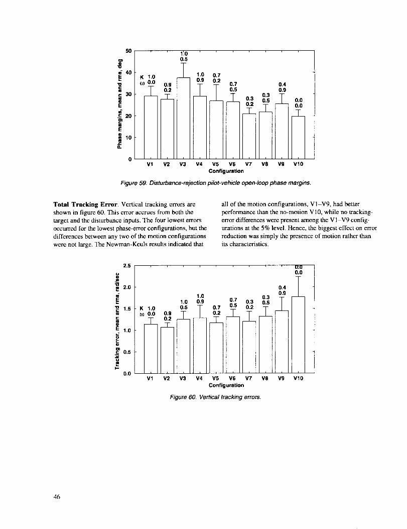
5O

O"O

40E113CIIS

c 30Q

EW

c 20

m

E

= 10M.1=D.

K 1.00.0

_L0.90.2

1'.00.5

0 I I I ,

Vl V2 V4

I

I

]V3

1.00.9

5_0.70.2

0.7

0.5i 0.30.2

1

V5 V6 V7

Configuration

0.40.9

0.3 T0.5 0.0

-]- 0.0

V8 V9 VIO

Figure 59. Disturbance-rejection pilot-vehicle open-loop phase margins.

Total Tracking Error. Vertical tracking errors are

shown in figure 60. This error accrues from both the

target and the disturbance inputs. The four lowest errors

occurred for the lowest phase-error configurations, but the

differences between any two of the motion configurations

were not large. The Newman-Keuls results indicated that

all of the motion configurations, V I-V9, had better

performance than the no-motion V I0, while no tracking-

error differences were present among the VI-V9 config-

urations at the 5% level. Hence, the biggest effect on error

reduction was simply the presence of motion rather than

its characteristics.

G1(D

C

EL..

(11

U

i"-

2.5

2.0

1.5 K 1.06O 0.0

__Z_1.0

0.5

0.0 'V1

0.90.2

V2

1.01.0 0.9 0.70.5 _ 0.7 0.5

_T_-- 02_T_

J J _ i i

V3 V4 V5 V6 V7

Configuration

Figure 60. Vertical tracking errors.

0.40.9

0.3 T0.3 0.5

o.g -I-

0.0

T

/

i i i

V8 V9 V10

46


Figure 61 provides the motion-fidelity ratings using the

definitions stated earlier. The ratings are divided into

"high," "medium," "low," and "split," where split refers to

a pilot assigning inconsistent ratings for repeated runs ofthe same configuration. Split ratings only occurred for the

VI configuration; this was more likely, because

configuration VI had more repeat evaluations than theother cases. The ratings indicate that no pilot perceived the

K = 0.3 cases to be high fidelity. Configuration V2

received the best overall ratings, and also had the lowest

mean tracking error as shown earlier. Configuration V3

surprisingly received two low ratings; V4 received no low

ratings. Configuration V6, which is essentially a combi-nation of the natural frequency of V3 and the gain of V5,

was rated worse than either V3 or V5. No configurations

in which the high-pass filter's high-frequency gain wasless than 0.3 was judged to be high fidelity. All pilots

rated the fixed-base condition to be low fidelity.

Summarizing the results of this section, the presence and

quality of motion influenced both target tracking and

disturbance rejection. Motion-filter natural frequency

affected both target tracking and disturbance rejection,

whereas motion gain affected only disturbance rejection.Overall, the results from this dual task are consistent with

those presented in section 4.

IVl0

Fixedbase

V9

L_

V8

I Io.o 0.2

High, Medium, Low,Split I

V4

V6

Medium

V5

I I0.4 o.6

Gain @ 1 rad/sec

8O

AO1

¢,)

so13

V3 '-

g40_

0

0V2 _

m

2o _.

I High

0.8 1.0

Figure 61. Pilot motion fidelity ratings for vertical task.

47

6. Vertical Experiment IIhAltitude and Altitude-Rate

Estimation

Background

Relative to flight, simulation has perennially producedless effective control of altitude and altitude rate. Fixed-

wing landings in simulation usually have higher runway

position dispersions and higher mean touchdown veloci-

ties than in flight. Bray showed that with a 16-in black-and-white television monitor, simulator vertical

displacements of at least +20 ft are required in order to

achieve the desired fidelity in the landing task (rcf. 60).

In helicopter simulations, pilots often comment that the

vertical damping (as perceived from the visual and motion

cues) is less than it is in flight (refs. 59, 63q55). Since

the math models have often been developed and validated

from in-flight measurements, attempts to determine thecause have focused on the simulator visual and motion

cues.

Often, the assumption is made that pilots obtain vehicle

acceleration information from the motion system, and rate

or position information from the visual system, as shown

in figure 62. Thus, decreasing motion gain or increasingwashout frequency is assumed not to affect the outer rate

and position loops. In this work, an experiment was

designed to test this assumption by exploring the effectsof visual scene properties and vertical motion on theestimation of altitude and altitude rate.

Experimental Setup

Five factors were incorporated in Vertical Experiment III:

(1) reposition direction, (2) initial altitude, (3) presence of

vertical motion, (4) visual scene level-of-detail control,

and (5) visual scene mean object size.

Tasks

The experiment involved two tasks.

1. In the first task, the altitude repositioning task, pilotswere instructed either to double or halve their initial

altitude. The initial altitudes were 15.6, 18.3, and

21.0 ft. Altitude was the only degree of freedom under

the pilot's control. No time requirement was placedon the task, and no requirements were imposed on

overshooting or undershooting what the pilots felt tobe their doubled (or halved) altitude.

2. In the second task, the altitude-rate control task,

pilots were instructed to climb or descend at aconstant rate of 3 ft/sec. The climbs started at an

altitude of 7.5 ft and ended at 42.5 ft. The descentsstarted at an altitude of 42.5 ft and ended at 7.5 ft.

These unusually specific altitudes were selected toallow one-to-one motion and visual cues in the

Vertical Motion Simulator.

For both tasks, all instruments were disabled so that

pilots would have to estimate their altitude and altitude

rate from the visual scene, motion system, or cockpit

collective movement. Although pilots would ordinarily

accomplish these tasks in flight by referring to aninstrument that measures either altitude or altitude rate,

these instruments were intentionally disabled so that the

possible value of the motion and visual cueing variationscould be determined.

T Acceleration Motion

cue I ,,,tem

Rate-of-climb and t Visual [_,altitude cues system

Figure 62. Typical assumptions in the apportioning ofsimulation cues.


The math model represented the AH-64 Apache helicopter:

[i_] I-0.122-ll81Ih]+F14.6][_c ] (18)i, =L 0.0 -12.9JLz, j L1.00j L •

The state z, was added to approximate the effects of

dynamic inflow into the rotor. All other displacements andorientations were held fixed at zero.


The simulator and cockpit were the same as for the yaw

experiment described in section 3. The Evans and

Sutherland CT5A visual system was used, but both thehardware and software were modified to achieve the visual

variations described below.

49

Design of Visual Scenes

Simulated scenes are typically less dense (fewer objects

per degree of field of view) at lower altitudes than at

higher altitudes. In flight, objects invisible at high

altitudes become visible at low altitudes, as the angle that

the object subtends at the eye becomes larger. When this

subtended angle exceeds an optical resolution threshold,

the object can be seen. These changes in detail cannot be

represented accurately owing to the required computational

load in the image generator. Instead, visual databases,

which are sets of objects, are stored and then faded in and

out of the scene according to range. This fading is adjusted

so that the transitions between databases appear natural.

How an image generator accomplishes this fading of

objects is called "level-of-detail management."

For this experiment, visual databases were constructed of

green polygons on a brown ground plane. These polygons

were randomly positioned at locations within a 430-ftradius forward of the aircraft. Each database was associated

with a particular altitude band (2.5-ft band). These bandsoccurred between altitudes of 5 and 45 ft. As the vehicle

moved between these 2.5-ft altitude bands, one database

smoothly faded out while the new database faded in.

For each altitude, whether or not a polygon was displayed

at that altitude depended on which of two visual thresholdswas used. The "small" visual threshold allowed objects to

be drawn when their vertical visual angle spanned at least

0.1 °; the "large" visual threshold allowed objects to bedrawn when their vertical visual angles spanned 0.2 ° .

In either case, the polygons were all rendered in a commonset. That is, the polygons were all distributed on a ground

plane; whether or not they were then drawn depended onthe visual threshold used. Thus, at the 0.1 o threshold,

more polygons wcrc drawn than in the 0.2 ° threshold. Thepolygons that would appear in the 0.2 ° threshold would

also appear at the 0.1 o threshold. Four different ground

planes of polygons, two each for the two visual

thresholds, were used so that any effects found would notbe due to some unfortuitous and unusual random

placement of the polygons.

Three levels of "level-of-detail management" were

evaluated: high, medium, and low. For the high condition,

62 polygon sizes were distributed exponentially in thedatabase with diameters between 0.025 ft and 17.23 ft.

The exponential spread was determined according to therelation

d i =17.23(0.9) i I=0,1 ..... 61 (19)

where di is the diameter of the ith polygon.

These 62 polygon sizes were placed in the common

database in the following manner. First, the largest

polygons were randomly placed until a specified portion of

the unfilled area was filled. Then, polygons of the next

largest size were randomly placed in the remaining area

until that same proportion of the unfilled area was filled.

This continued, allowing no overlapping regions, until

polygons of all 62 sizes were placed. Since the image

generator could display a maximum of 1350 polygons at

60 Hz, the proportion parameter was selected such thatthis maximum was not exceeded.

For the medium condition, the polygon sizes were

distributed evenly, not exponentially, between 0.025 ft

and 17.23 ft. For the low condition, only a single database

was presented at all altitudes, so no fading in and out

occurred. For the low condition, two sets of only three

polygon sizes were used: one set had polygon diameters of

3, 5.23, and 7.46 ft. The other set had polygon diameters

of 6, 10.45, and 14.9 ft. These sizes were chosen using

the following rationale. First, the largest polygons in each

set spanned 0.1 and 0.2 visual degrees at the 45-ft altitude.

Second, the smallest polygon in the large set of sizes

spanned approximately twice as much visual angle as the

small polygon in the small set.

Analytical Evaluation of Visual Scenes

Several metrics were used to evaluate the efficacy of using

these procedures in constructing the databases. First, the

number of visible polygons is plotted for each of three 10°

elevation bands (in fig. 63). These three 10° elevation

bands between 0 ° and 30° below the horizon nearly span

the field of view represented by the cockpit windows. As

shown, in the high condition, the number of polygons

visible is nearly constant versus altitude for each elevation

band. However, it is difficult to compare the medium and

low condition in terms of the level-of-detail represented.

For the medium condition, the number of polygons

visible always increases with altitude, but in the low

condition, the number of polygons in the 0°-10 ° elevationband decreases with increasing altitude.

5O

LODconstancy

1_i --High

....................... ---- Medium

1 ...............::::S,ow

| 0°- 10° degrees

.._ 600 _ below horizon.....

o5 45

900 T 10°-20°

600 T below horizon . _...._.""' _ - P

_ O_"6Q.

"_ 20°- 30*

0 --J:2-5 45

Altitude,ft Altitude,ft

Figure 63. Visible polygons for the three level-of-detail visual databases.

Another metric, mean visual form ratio, was also

examined. Mean visual form ratio is the average angular

width divided by angular length. It is simply a function of

altitude and range to an object. Figure 64 shows that the

mean form ratio was invariant for the high condition,

decreased slightly with altitude for the medium condition,

and dramatically decreased with altitude for the lowcondition.


Two motion configurations were presented: full motionand no motion.

Procedure

Five NASA Ames test pilots flew the two tasks. All of

the pilots had extensive rotorcraft and simulation experi-

ence. Pilots signaled the initiation and conclusion of the

task by pulling a trigger on the centerstick. The pilots

solo 40

EO

u- 20_

oi

\\

\

LODcoherency.........Low

.... Medium

-- High

""....

5 45Altitude,ft

Figure 64. Mean visual form ratio for the three level-of-detail visual databases.

participated in one or two sessions per day, with each

session lasting 1 to 2 hr. Pilots received training duringtheir first session and a short refamiliarization on subse-

quent sessions. These training sessions used several high

level-of-detail databases constructed especially for training

purposes (they were not used in the data collection). Pilotsevaluated the configurations in a randomized order.

Results: Objective Performance Data

All of the results for the altitude repositioning task were

analyzed using a repeated measures analysis of variance(ref. 54). For this task, the pilot's altitude repositioning

error was determined by

actual altitude change 1

- desired altitude changeJ% repositioning error --

desired altitude change

(20)

Figure 65 shows the mean percent repositioning error for

three of the five experimental factors: vertical motion

presence, reposition direction, and initial altitude. Across

all visual databases, accuracy in altitude repositioning

improved when motion was present (F(1,4) = 39.347,

p = 0.003), with an overall tendency to overshoot the

desired altitude change. This result was very surprising,for conventional wisdom would suggest that estimating

the required altitude change would be a purely visual task.

It would be expected, based on the results of Vertical

Experiments I and II, that the trajectory quality betweenthe two final altitude points would be improved with

motion (motion allowing the generation of lead, thus

improving the open-loop phase margin). However, it was

not expected that the presence of motion would affect the

51

¢.

P

O.

60*

40

2O

-20

Double

Absent I

|Halve

_15.671633

Motion Repoettiondirection

Initial

altitude

Figure 65. Altitude repositioning error.

altitude endpoint. Apparently the pilot was combining the

visual and motion cues in a way that improved his

estimate of the vehicle's state.

In comparing climbs versus descents, pilots were better at

halving the altitude than they were at doubling it (F(1,4) =

23.339, p = 0.008); there was a tendency to ascend too

high when doubling altitude and to descend too little when

halving altitude. Finally, figure 65 shows that better

accuracy resulted when starting at higher initial altitudes

(F(1,4) = 14.064, p = 0.002); there was an overall

tendency to overshoot the desired altitude. Interestingly,

there were no statistically significant main effects found

when varying the level-of-detail quality among the

databases, nor for the minimum resolution size.

No main effects were found for visual scene level-of-detail

manipulations, but there was a statistically significant

interaction between level-of-detail and initial altitude

(F(4,16) = 3.451, p = 0.032). Figure 66 illustrates this

interaction. For the ascents, the final altitude more closely

matches the desired doubled altitude as the level-of-detail

becomes more constant. Only for the 21-ft initial-altitude

descents did the high constancy level-of-detail database not

result in the best repositioning performance. So, it

appears useful to attempt to have the visual system mimic

the level-of-detail changes, as one would experience in the

real world.

Altitude-Rate Control Task. The performance

measurement for the altitude-rate control task was mean

absolute vertical rate during the climb or descent. Only

data between vehicle altitudes of ] 0 and 40 ft were used,

thus eliminating the initiation of either the climb or the

descent.

55-

5O

45

40

35

Initial altitude• 15.67• 18.33

-. • 21.oo

........7_".....................l ................."_"........ Double 21.00IM

•............................................r......... Double 16.33

....................................................................Double 15.67

10 ¸i O

.....................................i .............21.oo........_...................+....................'t .........Half 10.33....................................................................Hal f 15.67

Low Medium HighLOD constancy

Figure 66. Altitude reposition versus level-of-detail and

initial altitude.

RepoeltionlnginslructionB

[ , °-°-°

_. t A:gned

3.00 ............................................. eed

>_ 2.50

2.00Abeent Preeent

Platform motion

Figure 67. Vertical speed dependence on motion and

movement direction.

Statistically, there were significant effects for the presence

of vertical platform motion (F(I,4) = 78.846, p = 0.001)

and for movement direction (F(I,4) = 14.806, p = 0.018).

There was also a significant interaction between these two

factors (F(I,4) = 12.379, p = 0.024). Figure 67 shows

these effects. Note that the vertical rates were slower with

motion than without motion, and that the vertical rates

were slower when descending than when climbing. Thc

presence or absence of platform motion had a stronger

effect on performance than the movement direction.

52

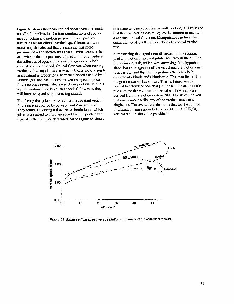
Figure 68 shows the mean vertical speeds versus altitudefor all of the pilots for the four combinations of move-

ment direction and motion presence. These profiles

illustrate that for climbs, vertical speed increased with

increasing altitude, and that the increase was more

pronounced when motion was absent. What seems to be

occurring is that the presence of platform motion reducesthe influence of optical flow rate changes on a pilot's

control of vertical speed. Optical flow rate when moving

vertically (the angular rate at which objects move visually

in elevation) is proportional to vertical speed divided byaltitude (ref. 66). So, at constant vertical speed, optical

flow rate continuously decreases during a climb. If pilots

try to maintain a nearly constant optical flow rate, they

will increase speed with increasing altitude.

The theory that pilots try to maintain a constant optical

flow rate is supported by Johnson and Awe (ref. 67).

They found that during a fixed-base simulation in which

pilots were asked to maintain speed that the pilots oftenslowed as their altitude decreased. Since Figure 68 shows

this same tendency, but less so with motion, it is believedthat the acceleration cue mitigates the attempt to maintain

a constant optical flow rate. Manipulations in level-of-

detail did not affect the pilots' ability to control verticalrate.

Summarizing the experiment discussed in this section,

platform motion improved pilots' accuracy in the altitude

repositioning task, which was surprising. It is hypothe-

sized that an integration of the visual and the motion cues

is occurring, and that the integration affects a pilot's

estimate of altitude and altitude rate. The specifics of this

integration are still unknown. That is, future work is

needed to determine how many of the altitude and altitude-

rate cues are derived from the visual and how many are

derived from the motion system. Still, this study showed

that one cannot ascribe any of the vertical states to a

single cue. The overall conclusion is that for the control

of altitude in simulation to be more like that of flight,

vertical motion should be provided.

6.00

4.00¸

O

"wo 2.00¸

0.0010

_"_" NNC

..,,-_z.-- _ - _- ..... Moil \,,, .....,,: .............................................Qn Descend

_, .. ...... .°.°°..I ..........--:,;;......

15 20 25 30 35Altitude.ft

Figure 68. Mean vertical speed versus platform motion and movement direction.

53

7. Roll-Lateral Experiment

Background

In flight simulation, the roll and lateral translational

degrees of freedom are treated together for several reasons.

First, owing to the motion platform geometry, a certain

amount of lateral translational motion must accompany a

rolling motion to locate the center of rotation properly.Second, for coordinated maneuvers, in which the body-axis

lateral aero-propulsive forces are zero, lateral translational

platform motion provides an acceleration to counteract the"leans" that would result from only rolling the cockpit.

Figure 69 shows a coordinated and an extremelyuncoordinated case (roll only) with a pendulum hanging

from the top of a rolling flight simulator cockpit. In bothcases, altitude remains constant. In the coordinated case,

the platform moves laterally with an acceleration of

g*tan_,t; however, the body-axis lateral component ofthe aero-propulsive force is zero which keeps ay = O.

Sustaining the platform acceleration to maintain thiscoordination consumes available lateral displacement

quickly.

Coordinated Uncoordinated

_plat Qplat

/ ! /Y'_Plat= gtan_pi'7. JD/Yp'at=O

/_J/_OcockPit g_'_sin(_plat

Figure 69. Coordinated vs. uncoordinated flight.

Most motion-base flight simulators are hexapods with

similar displacement capabilities. In these devices,sufficient lateral translational platform travel is not

available to simulate exactly the motion cues that a pilot

would receive in coordinated flight. To reduce the amount

of lateral displacement used, platform drivc commands useseveral methods. In one method, the roll angle of the

motion platform is reduced relative to the model (and thusthe visual scene). This requires less lateral travel, since

less lean-due-to-roll motion is present. In the second

method, less than the full amount of lateral translational

motion required for coordination is used. The purpose of

his study was to investigate the trade-off between these

two options.

Experimental Setup

Task

Constant-altitude lateral side steps were performed between

two points 20 ft apart. A positioning sight in the visual

scene allowed pilots to use parallax to determine their

positioning error precisely. The desired positioning

performance standard was +3 ft about the desired hover

point (which was 20 ft away), and the adequate perfor-mance standard was +8 ft. The task had to be completed in

less than ! 0 sec for desired performance and in less than

15 sec for adequate performance. Pilots pressed an eventmarker on the center stick when they felt they had acquired

the station-keeping point. They were instructed that push-

ing this button meant that they were within the position

error for desired performance, and that they believed they

would remain within the desired performance standard.


The math model had only two degrees of freedom. Altitude

remained constant at 25 ft; heading, pitch, and

longitudinal position remained constant at zero. Pilots

controlled the vehicle with lateral displacements of a

center stick only. The equations for motion were

= --4.5_ + 1.7_la t (21)

_,= g sin _ (22)

where v is the body-fixed velocity in the y direction

(lateral). These equations represent a typical helicopter

math model that is fully coordinated at the aircraft's

c.m., since no lateral aero-propulsive forces are present

( ay = _, - g sin ¢). Actual helicopters have a drag owing tolateral translational velocity, and they also produce a sideforce at the rotor which contributes to a rolling moment.

Each of these real-world effects causes uncoordinated flight

during a side-step maneuver. This experiment used a fully

coordinated model, since the objective was to examine theeffects of uncoordinated simulation cues caused by simu-

lator platform displacement limitations. Thus, these real-world effects were intentionally absent. So the model

represented a vehicle in which only applied torques created

rolling motion (similar to an AV-8B-like concept) with

no drag owing to velocity (which is small near hover).

For the experiment, the pilot's abdomen was located at theaircraft's c.m. The roll-axis dynamics given above, when

combined with the visual system delay of 60 msec, had

55

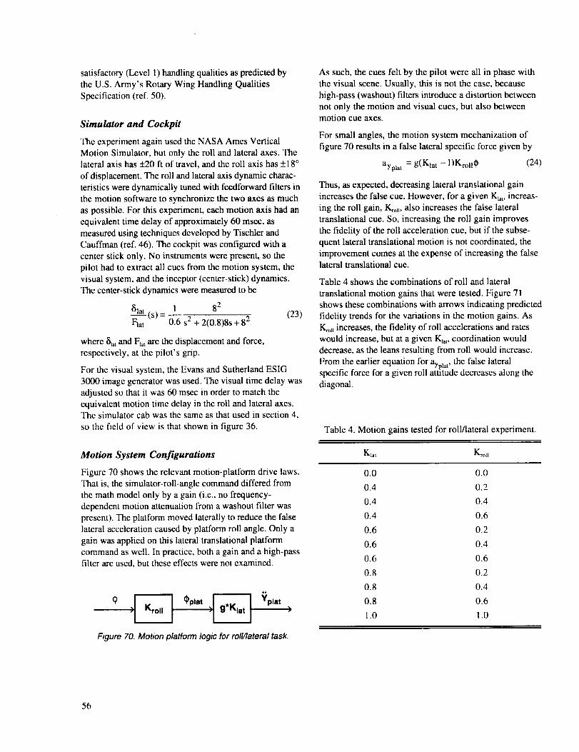
satisfactory(Level1)handlingqualitiesaspredictedbytheU.S.Army'sRotaryWingHandlingQualitiesSpecification(ref.50).


The experiment again used the NASA Ames Vertical

Motion Simulator, but only the roll and lateral axes. Thelateral axis has +20 ft of travel, and the roll axis has +18 °

of displacement. The roll and lateral axis dynamic charac-

teristics were dynamically tuned with feedforward filters in

the motion software to synchronize the two axes as much

as possible. For this experiment, each motion axis had an

equivalent time delay of approximately 60 msec, as

measured using techniques developed by Tischler and

Cauffman (ref. 46). The cockpit was configured with a

center stick only. No instruments were present, so the

pilot had to extract all cues from the motion system, the

visual system, and the inceptor (center-stick) dynamics.

The center-stick dynamics were measured to be

Slat (s)= 1 8 2 (23)Fla t 0.6 s 2 + 2(0.8)8s + 8 2

where _,t and F_at are the displacement and force,

respectively, at the pilot's grip.

For the visual system, the Evans and Sutherland ESIG

3000 image generator was used. The visual time delay was

adjusted so that it was 60 msec in order to match the

equivalent motion time delay in the roll and lateral axes.The simulator cab was the same as that used in section 4,

so the field of view is that shown in figure 36.


Figure 70 shows the relevant motion-platform drive laws.

That is, the simulator-roll-angle command differed from

the math model only by a gain (i.e., no frequency-

dependent motion attenuation from a washout filter was

present). The platform moved laterally to reduce the false

lateral acceleration caused by platform roll angle. Only a

gain was applied on this lateral translational platform

command as well. In practice, both a gain and a high-passfilter are used, but these effects were not examined.

o,

Figure 70. Motion platform logic for roll�lateral task.

As such, the cues felt by the pilot were all in phase with

the visual scene. Usually, this is not the case, because

high-pass (washout) filters introduce a distortion between

not only the motion and visual cues, but also betweenmotion cue axes.

For small angles, the motion system mechanization of

figure 70 results in a false lateral specific force given by

ayplat = g(Kla t - l)Kroll 0 (24)

Thus, as expected, decreasing lateral translational gain

increases the false cue. However, for a given K_,L,increas-

ing the roll gain, I_,, also increases the false lateral

translational cue. So, increasing the roll gain improves

the fidelity of the roll acceleration cue, but if the subse-

quent lateral translational motion is not coordinated, the

improvement comes at the expense of increasing the falselateral translational cue.

Table 4 shows the combinations of roll and lateral

translational motion gains that were tested. Figure 71shows these combinations with arrows indicating predicted

fidelity trends for the variations in the motion gains. As

K_H increases, the fidelity of roll accelerations and rates

would increase, but at a given KI_,, coordination would

decrease, as the leans resulting from roll would increase.

From the earlier equation for ay 1 ' the false lateralpa2

specific force for a given roll attitude decreases along the

diagonal.

Table 4. Motion gains tested for roll/lateral experiment.

Klat Kroll

0.0 0.0

0.4 0.2

0.4 0.4

0.4 0.6

0.6 0.2

0.6 0.4

0.6 0.6

0.8 0.2

0.8 0.4

0.8 0.6

1.0 1.0

56

1.0 -- •

Kroll

0.8 --

0.6 i

0,4 --

0,2 m

Increasing roll fidelity

• •Increasing

• _coordinati;n

:0.0 = l I I I I

0.0 0.2 0.4 0.6 0.8 1.0

Klat

Figure 71. Configurations and fidelity effects for roll/lateral

experiment.

Procedure

Three test pilots participated in the study. The pilots werefrom NASA Ames, the Federal Aviation Administration,

and Lockheed-Martin. All pilots had significant flight and

simulation experience. The NASA and the FAA pilot had

extensive helicopter experience, and the Lockheed Martin

pilot had experience in hovering jet aircraft.

Pilots practiced with a motion configuration selected

randomly at the beginning of each test period. During the

trials, each of the three pilots evaluated the configurations

in a random order. Pilots rated each configuration after

performing the task with that configuration three times.

Pilots subjectively evaluated the configurations in two

categories: motion fidelity and handling qualities. For

motion fidelity, they used the scale developed by Sinacori

(ref. 44), but with the modifications suggested in Vertical

Experiment I. The scale is shown in table 5. To rate the

handling qualities, the Cooper-Harper scale was used

(ref. 53). An overview of the scale is given in

appendix D.

Table 5. Revised motion fidelity scale.

Fidelity rating Definition

High Motion sensations are likethose of flight

Motion sensations are

noticeably different from

flight, but not objectionable

Low Motion sensations are

noticeably different from

flight and are objectionable

Medium

Results


Again, compelling performance differences occurredbetween full motion and no motion, as shown in

figure 72. The solid lines in the figure represent fullmotion (K_ = K_L = 1), and the dotted lines represent no

motion. When transitioning from full to no motion,

performance degraded, and the magnitude and rate ofcontrol inputs increased. Pilot-vehicle performance degra-

dation typically becomes more marked as the dependency

on the pilot for control and stabilization increases. The

magnitude and rate of control input increases, because the

pilot is now trying to extract vehicle state informationkinesthetically (via sensing position and forces in the

limb-manipulator system), since the platform cues that

supplied lead information directly (from vehicle accelera-tion) are now missing. These tendencies are consistent

with the other studies in this report.

Figure 73 illustrates how overall positioning performancevaried with the configurations. Pilots assigned numerical

values to designate performance levels: a 1 for desired

performance; a 2 for adequate performance; and a 3 for

inadequate performance. Since pilots flew three runs for

each configuration, their performance for each one of the

three runs was assigned a value. Thus, if adequate perfor-mance was achieved on all three runs, thc score was 6.

Mean and standard deviations are shown.

57

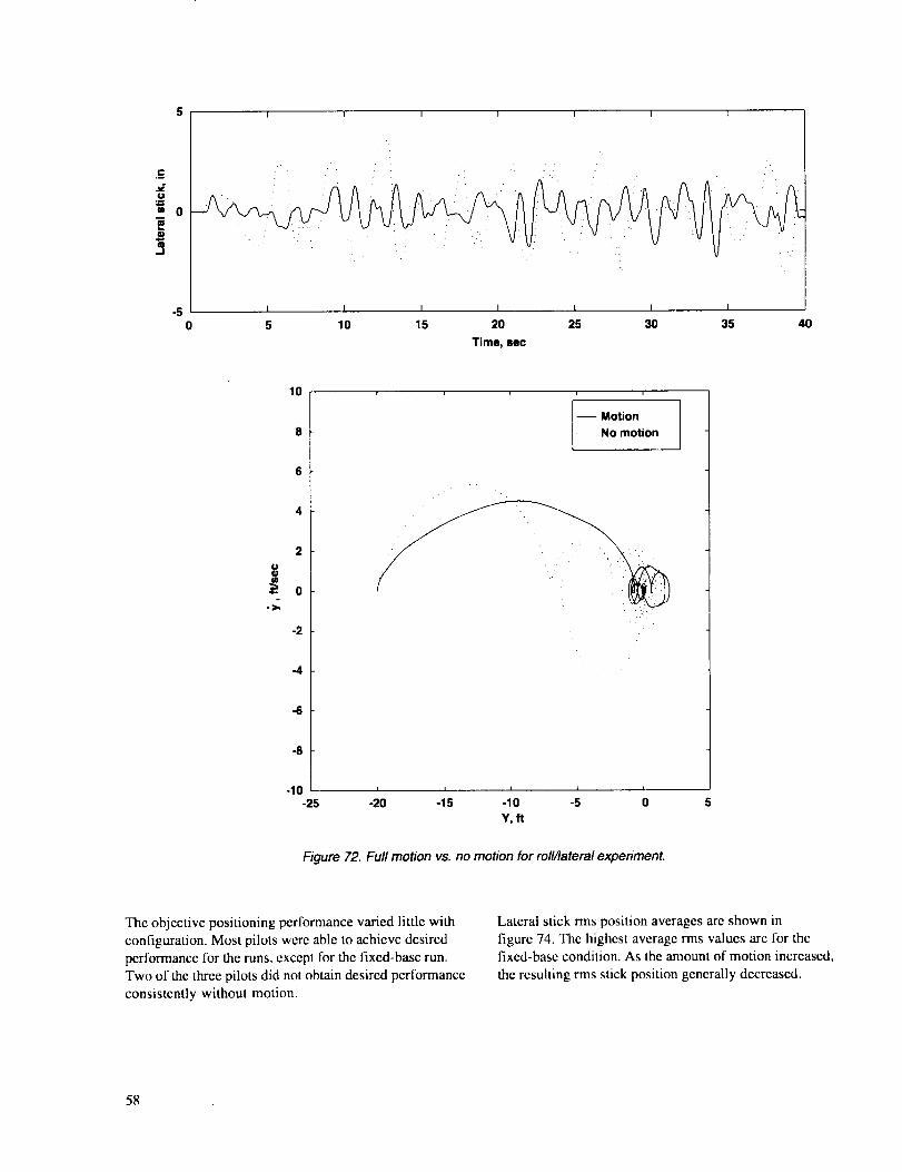
5 I I I I I l 1

.c

III--I

-50

• .h.'.

I I I I I I I

5 10 15 20 25 30 35

Time, sec

h

4O

OO

I0 i i

Motion

No motion

0

-2

-4

-6

-8

-10 ' ' ' _ '-25 -20 -15 -10 -5 0

Y, fl

Figure 72. Full motion vs. no motion for roll/lateral experiment.

The objective posluoning performance varied little with

configuration. Most pilots were able to achieve desired

performance for the runs, except for the fixed-base run.

Two of the three pilots did not obtain desired performance

consistently without motion.

Lateral stick rms position averages are shown in

figure 74. The highest average rms values arc for the

fixed-base condition. As the amount of motion increased,

the resulting rms stick position generally decreased.

58

£v

1.0

0.8

0.6

0.4

0.2

0.0

3 - Average(3) - Std. dev. J

3.67

(0.58)

0.0

3.17 3.00 3.00(0.29) (0.00) (0.00)

3.33 3.33 3.00(0.57) (0.57) (0.00)

3.00 3.00 3.17(0.00) (0.00) (0.29)

' t I I II

0.2 0.4 0.6 0.8 1.0

Klat

Figure 73. Positioning performance for roll/lateral

experiment.

3.00(0.00)

ov

1.0

I 3 -Average I(3) - Std. dev.

0.8

0.6

0.4

0.2

2.95

0.0 11"10) I

0.0 0.2

3.45 2.64 2.53(1.97) (0.81) (1.38)

2.98 3.33 2.72(1.24) (1.62) (1.46)

2.57 3.23 3.33(0.95) (1.62) (1.55)

2.18(0.77)

I I I I0.4 0.6 0.8 1.0

Klat

Figure 75. Rms lateral stick rate for roll/lateral experiment

(in/sec).

£

1.0

J 3 - Average ](3) - Std. dev.

0.8

0.6

0.4

0.2

0.88

0.0 (0"35) I

0.0 0.2

0.79 0.65 0.60(0.37) (0.16) (0.21)

0.77 0.80 0.68

(0.26) (0.31) (0.29)

0.69 0.86 0.81(0.17) (0.41) (0.27)

I I I I0.4 0.6 0.8 1.0

Klat

Figure 74. Rms lateral stick position for roll/lateral

experiment (in.).

0.51(0.12)

Figure 75 shows how rms of the lateral stick rate varied

over the configurations. Each value represents the average

of the three rms values (one for each pilot) for a concate-

nation of three time-histories (one for each run). The

fixed-base condition resulted in higher rms stick rates than

the larger motion conditions (Kla t = l/Kroll = l; KI_ =

0.8/K,oii = 0.6; Klat = 0.8/I_oll = 0.4; Klat = 0-6/K_oll =

0.6). Comparisons with and among the remaining

configurations are less clear.


Figure 76 shows how the motion fidelity ratings changed

versus roll gain and lateral translational gain. Numerical

values of 1, 2, and 3 were assigned to fidelity ratings of

Low, Medium, and High for determining the averages. All

pilots rated the fidelity of the fixed-base case as Low. In

general, as the amount of motion increased (increasing

both K_a, and K=H) the rated motion fidelity improved.

Interestingly, as K_,,H increased for a fixed Klat, fidelity

improved. This situation increases the false lateral specific

force cue, which would suggest a fidelity degradation.

However, it appears this degradation was more than

compensated for by an increase in roll fidelity.

ov

1.0 2.00(0.50)3 - Average I(3) - Std. dev.

0.8

0.6

0.4

0,2

1.00

0.0 110"00)

0.0

1.33 1.89 2.67(0.58) (0.19) (0.57)

1.00 1.67 2.00

(0.00) (0.58) (0.00)

1.50 1.00 1.17(0.87) (0.00) (0.29)

I I I I I0.2 0.4 0.6 0.8 1.0

Klat

Figure 76. Motion fidelity ratings for roll/lateral experiment.

59

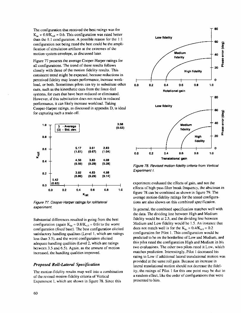
The configuration that received the best ratings was for

K_., = 0.8/K_, = 0.6. This configuration was rated better

than the 1:1 configuration. A possible reason for the 1: 1

configuration not being rated the best could be the ampli-fication of simulation artifacts at the extremes of the

motion-system envelope, as discussed later.

Figure 77 presents the average Cooper-Harper ratings for

all configurations. The trend of these results follows

closely with those of the motion fidelity results. This

consistent trend might be expected, because reductions in

perceived fidelity may lessen performance, increase work-load, or both. Sometimes pilots can try to substitute other

cues, such as the kinesthetic cues from the force-feel

systems, for cues that have been reduced or eliminated.However, if this substitution does not result in reduced

performance, it can likely increase workload. Taking

Cooper-Harper ratings, as discussed in appendix D, is ideal

for capturing such a trade-off.

1.0 3.58(0.s2)

0.8

0.6

0.4

0.2

0.0

3 - Average(3) - Std. dev.

5.42

(0.63)

0.0

5.17 3.61 2.83

(1.61) (0.67) (1.04)

4.50 3.83 4.08

(0.50) (0.29) (0.58)

3.92 4.83 4.58

(0.80) (0.29) (0.14)

I I I I I0.2 0.4 0.6 0.8 1.0

Klat

Figure 77. Cooper-Harper ratings for roll�lateral

experiment.

Substantial differences resulted in going from the best

configuration (again K_,, -- 0,8/K_o, = 0.6) to the worst

configuration (fixed base). The best configuration elicited

satisfactory handling qualities (Level 1, which are ratings

less than 3.5), and the worst configuration elicited

adequate handling qualities (Level 2, which are ratings

between 3.5 and 6.5). Again, as the amount of motion

increased, the handling qualities improved.

Proposed Roll-Lateral Specification

Thc motion-fidelity results map well into a combination

of the revised motion-fidelity criteria of Vertical

Experiment I, which are shown in figure 78. Since this

Low fidelity

/ / "'°'"°',, "0.0 0.2 0.4 0.6 0.8 1.0

Rotational gain

-80

-80

Low fidelity

- 411

/ / High 20

/ / T o0.0 0.2 0.4 0.6 0.8 1.0

Translational gain

Figure 78. Revised motion fidelity criteria from Vertical

Experiment I.

60 A

20

0

AolO

m

r"

n

experiment evaluated the effects of gain, and not the

effects of high-pass filter break frequency, the abscissas in

figure 78 can be combined as shown in figure 79. The

average motion-fidelity ratings for the tested configura-

tions are also shown on this combined specification.

In general, the combined specification matches well with

the data. The dividing line between High and Medium

fidelity would be at 2.5, and the dividing line between

Medium and Low fidelity would be 1.5. An instance thatdoes not match well is for the K_,, = 0.4/Kro]l : 0.2

configuration for Pilot 1. This configuration would be

predicted to be on the borderline of Low and Medium, and

this pilot rated the configuration High and Medium in his

two evaluations. The other two pilots rated it Low, which

matches prediction. Interestingly, Pilot 1 decreased his

rating to Low if additional lateral translational motion was

provided at the same roll gain. Because an increase inlateral translational motion should not decrease the fidel-

ity, the ratings of Pilot 1 for this one point may be due toa random effect, like the order of configurations that were

presented to him.

60

.o

1.0

I 3 - Average(3) - Std. dev.

0.8

0.6

0.4

0.2

1.00

0.0 (0"00) I

0.0 0.2

Low

fidelity

liMedium I High

Ifidelity I fidelity

I I

1_3 1._9 2.67(0 8) (0.19) (0.57)

1._)0 1._7 2.00 -- --

(o]oo) (o._ ---(o_

lJ50 1.00 1.17

(o._/_- -_.o-o3--(o_

I I t I0.4 0.6 0.8 1.0

Klat

2.00(0.50)

Figure 79. Proposed combined specification for m/I/lateral

gains.

The second poor match is for the full-motion (K_a, =

0.4/K_o_ = 0.2) configuration. On average, the pilots rated

the fidelity of this configuration Medium. A possible

reason that Medium, instead of High, ratings were given

is that some of the undesired side-effects of providing

extremely large motion were noticed. An example of a

VMS artifact is the rack-and-pinion noise that is propor-

tional to lateral-track velocity. Pilots commented on the

noise, and since it represents a sensation noticeably

different from flight, a rating of Medium fidelity results.

Since the K_a_= 0.8/K_oH = 0.6 configuration effectively

results in 48% of the lateral translational motion used in

the 1: 1 case, artifacts such as the above are reduced

significantly. Another possible side-effect is the imperfect

high-frequency coordination between the roll and lateral

axes; for high-frequency tracking, using high gains can

reveal a noticeable, but not objectionable, sensation (i.e.,

the definition of Medium fidelity). Still, with these two

exceptions, the criterion in figure 79 correlates well with

the data.

61

8. Discussion of Overall Results

General Discussion

These experiments showed the powerful effect that

platform motion has on pilot-vehicle performance and on

pilot opinion in flight simulation. Often, the quantitativemeasures have supported the pilot's subjective measures,

which adds confidence to the results. In addition,

frequency-response analyses offer an explanation of howthe characteristics of the motion filter affect closed-loop

performance.

The powerful effect of motion was shown even when the

pilot was creating his own motion, which was the case in

all of the tasks except the disturbance-rejection taskdiscussed in section 5. This result conflicts with the views

of Hunter et al. (ref. 14) and Puig et al. (ref. 15). Thedifference between these two views is almost certainly a

result of differences in vehicle dynamics. At low speed,

fixed-wing aircraft on stabilized paths do not require as

much compensation from a pilot as do helicopters. In

addition, the tasks that helicopters perform often require

the pilot to control all six degrees of freedom of the

vehicle simultaneously. Improved fidelity of external cues,

such as motion cues, aid in the effective pilot control of

the vehicle. Thus, motion requirements cannot be defined

by task alone. Both the task and the vehicle must beconsidered in concert.

This report has illustrated the performance and opinion

differences that arise when simulator motion is provided,

but it has not shown if there is any training benefit to the

use of motion. It is possible that training in a more

difficult task environment (no motion) may actually

shorten or improve training. For instance, learning to

balance a short inverted pendulum can train a person to

balance a long inverted pendulum easily. However, if lackof motion causes a bad habit to be learned, then that

would certainly argue against training without motion.

The effectiveness of training without motion would

require a careful transfer-of-training study.

Among the motion configurations tested, it was thetranslational motion that always had a strong effect. Yaw

rotational motion was shown to be a redundant cue, and

less roll motion was more acceptable (when comparing

percent of full motion) than less lateral translational

motion. Requiring less motion in the rotational axes isstill consistent with the revised set of the Sinacori criteria

that were suggested in this report.

A question arises as to why only one of the threerotational cues is redundant. That is, why is yaw rota-

tional motion redundant, but pitch and roll motion useful?

A possibility is that the pitch and roll rotational cues (as

sensed by the inner ear) are no more important than the

yaw rotational cue, yet their usefulness arises from the

additional cues concomitant with pitch and roll motion.These additional cues have two sources.

First, pitch and roll motion cues interact with the gravity

vector, as discussed in section 7. Very few simulators can

remove the specific force cue that arises from either pitch

or roll attitude. As such, evaluating the effect of the

angular cue only is challenging; it has only been investi-

gated by Jex et at. (ref. 41) in which subjects rolled while

lying on their backs (thus the gravity vector did not

change relative orientation during an orientation).

Although that study showed an effect of roll, this could bedue to another factor (in addition, it might be argued that

compelling roll visual cues were not present in that study,

as only a horizon line was present).

The other factor is the tangential acceleration that resultsfrom the moment ann between the roll center of rotation

and the motion sensors on a human. It is not possible to

eliminate the effect of these tangential accelerations

completely, for the human motion sensors are in different

locations (inner ear, neck, buttocks, limbs). Some

experiments have isolated the head by fixing it in an

apparatus and subsequently performing reorientationsabout that axis, but those were not piloted experiments.

Thus, when pitching and rolling, isolating the angular cuefrom the translational cue is difficult if not impossible. It

is only in yaw that many of these cross-coupling effectsinto the translational axes are lessened (but perhaps not

removed completely, as discussed in sec. 3). Thus, the

above reasons may explain why the requirements on the

yaw axis are different from pitch and roll.

Although the longitudinal axis was not examined in thesestudies, no reason is offered as to why the requirements in

that axis might be different from those in either vertical orlateral translation.

63

Proposed Fidelity Criteria versus

Results of Previous Research

Since a cornerstone of the results presented herein was the

modification and validation of the fidelity criteria in

figure 78, placing those criteria in the context of other

work is important. The results of previous work are

discussed in section 1, and figure 80 correlates the previ-

ous work with the new criteria suggested here. In

figure 80, the points tested and found to have at least

adequate fidelity are shown. The word "adequate" is chosenin an effort to make a consistent comparison with the

earlier work. Much of the earlier work attempts to define a

boundary between adequate and inadequate rather than

breaking down adequate into three categories such as High,

Medium, and Low fidelity. However, it is appropriate thatthe user should strive to stay away from Low fidelity,

which would certainly be termed as inadequate, for the

motion sensations are objectionable. Thus, in comparing

the previous work with the proposed criteria, an

inconsistency would be present if previous work stated

that an "adequate" motion system setup was in the

proposed Low fidelity region.

In the rotational axes, the criteria apply only to pitch and

roll; yaw was found to be redundant. Only the work of

Bergeron (ref. 38) evaluated a range of yaw configurations,which was discussed earlier. The only inconsistency

between the previous work and the criteria suggested is the

work by Shirachi and Shirley (ref. 42). Their experiment

did not vary motion-filter natural frequency, which

provided 62.5 ° of phase distortion at 1 rad/sec, which is2.5 ° in excess of the Medium fidelity boundary. Still, the

boundary at 60 ° should remain, for both the work of

Stapleford et al. (ref. 26) and Bray (ref. 27) support it. If

Shirachi and Shirley had evaluated conditions with less

phase distortion, those conditions might have been

preferred.

In the translational axes, a "region of uncertainty" extends

into the Low fidelity region; this does not suggest an

inconsistency, however, because that area simply was not

evaluated by Jex et al. (ref. 43). However, a "delayed side

force" region cuts off an area in Medium fidelity. The

delayed-side-force region applies to the sway axis when

that axis is used to eliminate the specific force that arises

from platform roll. That region was not explored in

section 7, and it may merit additional examination.

However, the delayed-side-force region is certainly adequate

when trying to represent true math model cues, as shown

in the vertical experiments discussed in sections 4 and 5.

There is another inconsistency in the translational axis

when compared to the results of Cooper and Howlett

(ref. 40). The displacement of their simulator was clearly

limited as shown by their boundary "too much displace-

ment." And their report states "Pilot criticism to motion

anomalies during returns from steady maneuvers still is a

problem." So, their region of "best compromise" is likely

to be based on their simulator's capability. It is interest-

ing to note that their rotational axis filter is well within

the High fidelity region. Since their platform is syner-

gistic (angular motion usurps translational motion and

vice versa), figure 80 suggests that they might relax their

angular motion in order to gain translational motion. This

change might allow both angular and translational axes tobe in the Medium fidelity region for some maneuvers,

rather than one in High and one in Low. The remaining

comparisons in figure 80 for the translational axes arefavorable. In general, the suggested criteria are reasonably

consistent with those of previous work.

64

100

LOW fidelity 80

Shirachi-Shirley (ref. 42)

cc cs_ 60

V van GOOI )400..

2O

' 0I

0.0 0.2 0.4 0.6 0.8 1.0

Rotational gain

Bestcompromise

_ Cooper-Howlett (40)_. 100t _ _ TOO much

Motion cues E,/_ _ _ I_,. displacementinadequate -----Im_ _ | I "1J/re. Cooper-Howlett (40)Cooper-Howlett (40) /j _ ,!p_____ 80

/I " I _1m-_./ "Delayed sidq rc(/. /" "| _ Jex, et al. (41) _"

_4 Regi°n JJd_"

LOW fidelitv40 o.

"Acce Bray (24)

_._ Jex -._'_ _'-_"The leans" 20

Jex, et el. (4.1) High fidelity)o much

displaceme

I Jex, et el. I 0

0.0 0,2 0.4 0.6 0.8 1,0

Rotational gain

Figure 80. Comparison of previous work with suggested criteria.

55

A General Method for Configuring

Motion Systems

Based on these experiments, on the experience attained in

their development, and on the discussion above, figure 81

suggests a step-by-step method for users who configure

motion systems. In figure 81, boxes that are dashed, and

underlined words in the boxes, represent suggested

additions to current practice as a result of the research

described in this report. This method is in contrast to the

current trial-and-error method that is often used by motion-

tuning experts and in subjective pilot evaluations. A

recent improvement to the trial-and-error method has been

suggested through the use of an expert system by Grantand Reid (refs. 68, 69). However, their method does not

explicitly use motion-fidelity criteria as does the method

proposed here.

First, the task needs to be analyzed to determine if

fundamental motion frequencies are present. Some tasks

have a predominant task frequency. For instance, nap-of-

the-Earth flight over regularly varying terrain cannecessitate low-frequency heave cues (the frequency

determined by hill separation divided by vehicle tbrward

speed). In these instances, the motion-filter natural

frequency and gain should not be set independently in an

attempt to satisfy the motion-fidelity criteria. Otherwise,

pilots do not feel like they are falling or climbing whenthe visual scene indicates they are falling or climbing.

Setting the motion-filter natural frequency should take

priority over setting the gain. The filter natural frequencyshould be selected such that less than a 30° phase error at

that predominant task frequency exists. Then, the motion

gain can be selected by trying to maximize the criteria

shown in figure 78. Once these two parameters are

selected, the motion-filter configuration should be

evaluated with a pilot flying the task in simulation todetermine if simulator excursions reach their physical

limits. If the physical displacement limits are reached,

Start

r

I Are there I

i fundamental motion II

I frequencies? J

Set motion gain and

natural frequency in

each axis per criteria

Yes [ Set motion system (_

I to give < 30 ° phaseerror there

l

Evaluate to

Set motion gain

per criteria

determine if you are

within motion limits

, , _No_ I Is motion fidelity acceptable? iI I

..I

_Yes

I Done

Figure 8 I. Method for configuring motion systems.

task

66

then the motion gain should be lowered until the ensuingmotion remains off the limits.

If fundamental motion frequencies do not exist, then the

gain and natural frequency of the motion filter can be set

independently. In this instance, the highest fidelity should

be sought in accordance with the criteria in figure 78.

Iteration with a pilot still needs to be performed to

determine the reachable fidelity level. At the end of either

of these paths, a certain achievable fidelity level will bereached.

If the desired fidelity level cannot be achieved for a given

simulator's displacement capability, then the user should

consider changing the task. Often the task is considered a

given and is treated as inviolate, since its origins may be

from flight test experience. However, trying to extrapolatesimulator results to flight when the simulator can only

duplicate the task with low fidelity will usually result in a

poor extrapolation.

Poor extrapolations from simulation to flight have

occurred frequently because of a control sensitivity that is

too high. Pilots improperly perceive vehicle sensitivity to

control stick inputs if tasks are not developed in concert

with a simulator's displacement capability. Rather than

change the task, the simulator's gain is reduced, which

gives the pilot a false reading of the true sensitivity.

If the process of developing a task is considered as a

feedback process with the attained simulator fidelity as a

performance metric, then modifying both the motion cuesand the task itself should be considered. It may be the only

method for achieving high simulation fidelity.

Extrapolations to flight can then be made with improvedconfidence.

Generally, this method should serve as a useful guide for

configuring motion systems and for selecting tasks tominimize differences between simulation and flight.

Although the method is iterative, it is possible that itscombination with the expert system ideas of Grant and

Reid (refs. 68, 69) might prove useful.

67

9. Conclusions

Summary

The five piloted helicopter simulation experiments

described in this report produced several important results.

Four of the six degrees of freedom were examined: roll,

yaw, lateral, and vertical. These experiments were

performed on the world's largest displacement flight

simulator, making it possible to perform many of the

tasks with the motion and visual cues matching exactly.

Using these experiments as a baseline allowed the effects

of degraded motion cues to be examined.

Representative helicopter math models were used; in somecases, the models were derived from flight test data.

Experienced test pilots were the experimental subjects, and

both objective and subjective data were employed in

developing the principal conclusions that follow.

1. Yaw rotational platform motion has no significant

effect on hovering flight simulation. The presence of

yaw platform rotational motion did not contribute to

significant improvements in pilot-vehicle perfor-

mance, control activity, pilot-rated compensation, or

pilot-rated motion fidelity.

2. Lateral translational platform motion has a significant

effect on hovering flight simulation. In contrast to

yaw rotational cues, the presence of lateral transla-

tional motion did contribute to improvements in

pilot-vehicle performance, reductions in control

activity, lower pilot-rated compensation, and higher

pilot-rated motion fidelity.

3. Lateral translational platform motion combined with

visual yaw cues made pilots believe yaw platform

rotational motion was present when it was not. This

visual and motion cueing combination gave pilots a

strong sensation that both rotational and lateraltranslational motions were present. It is believed that

more rapid vection was produced by the lateral

translational motion cue. Thus, for hovering flight

simulation, one should represent the lateral transla-

tional acceleration cue, for it is important to all the

aspects of pilot-vehicle performance and pilot

opinion. The same point cannot be made for yaw-axis

rotational motion. As such, since many of today's

hexapod motion platforms achieve both lateral

translational and yaw rotational motion with the same

set of limited-travel actuators, a high weighting

should be placed on representing the former cues

rather than the latter. An alternative to modifying

today's hexapod motion platforms is to develop a new

simulator configuration that emphasizes limited

translational motion. Because lateral and vertical

translational motions are the most prevalent, placinga cab on the end of a cantilevered arm that can rotate

in azimuth and elevation would provide these

motions. Different length arms could be used

depending on the vehicle capability, the evaluation

requirements, or both.

4. Vertical platform motion has a significant effect on

pilot-vehicle performance, control activity, and

motion fidelity. Pilots were surprised at the perfor-

mance results and at how their technique had to

change when all motion was removed. Two of the

three pilots made collective inputs in the wrong

direction when flying fixed base. Until the value of

vertical motion was demonstrated, pilot subjective

impressions were that the vertical task was primarily

visual. Thus, caution should be used when interpret-

ing piloted subjective impressions of the value ofmotion. From these vertical-axis results, a revised

specification was developed that better correlated with

existing experimental results.

5. Vertical motion cues affected altitude estimation.

Pilots, when asked to double or halve their altitude,

had their performance significantly affected by vertical

platform motion. With vertical motion, pilots more

accurately doubled and halved their altitude. Until

now, it was generally accepted that steady-state

altitude estimation was derived from visual cues only.

A hypothesis is that the pilot estimates vehicle state

using all the available sensory inputs. As a part of

this, some significant weighting is applied to

acceleration cues that provide a component of the

pilot's position estimate.

6. A specification for roll-lateral motion requirements

was developed. For a side-step task that exactly

reproduced motion and visual cues, significant

performance and opinion differences resulted asmotion was removed. A combination of translational

and rotational gain specifications provided a good

prediction of motion-fidelity ratings.

Recommendations for Future Work

Two additional degrees of freedom, pitch and surge,

should be examined. The results for these two coupled

axes are expected to be similar to those of

the coupled roll and lateral axes.

69

2. Thespecificationdemarcationsbetweenhigh,

medium, and low fidelity were determined based on

the granularity of the points tested. Further efforts areneeded to determine the curves that divide the fidelity

regions more precisely.

3. Controlled experiments should be performed on

several representative hexapod platforms to quantify

the performance benefits of allowing increased motion

in the other axes when turning the yaw rotational

displacement off.

4. Continued attempts should be made to model the

pilot-vehicle system in the simulator environment.Several unusual results, such as the performance

degradation with the addition of yaw rotational

motion and the improved estimation of height withthe addition of vertical motion have been shown here.

Future models need to account for these findings.

5. Does learning to fly a helicopter on a substandard or

suboptimal motion platform increase total training

costs, or does it pose a safety hazard? To answer these

questions, a careful transfer-of-training study needs to

be performed.

70

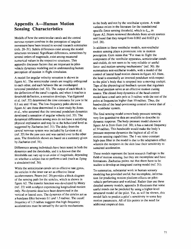
Appendix AmHuman Motion

Sensing Characteristics

Models of how the semicircular canals and the central

nervous system combine in the perception of angularmovement have been treated in several research summaries

(refs. 28-31). Subtle differences exist among the model

structures reviewed. Significant differences, sometimes by

several orders of magnitude, exist among measured

numerical values in the respective structures. This

appendix discusses factors that are important in pilot-

vehicle dynamics modeling and in understanding human

perception of motion in flight simulation.

A model for angular velocity sensation is shown in

figure A1. The semicircular canals are roughly orthogonalto each other, and each behaves like an overdamped

torsional pendulum (ref. 32). The output of each block is

the deflection of the canal' s cupula, and when it reaches a

threshold deflection, a sensation develops. Van Egmond

et al. (ref. 32) determined the time constants for yaw to be

0.1 sec and 10 sec. The low-frequency poles shown in

figure A 1 are those determined in a later study by Jones

et al., who assumed that the torsional pendulum dynamics

developed a sensation of angular velocity (ref. 33). The

dynamical differences among axes do not have a satisfying

physical explanation and may lie at the behavioral level as

suggested by Zacharias (ref. 3 !). The delay from the

central nervous system was included by Levison et al.

(ref. 35) for the yaw axis and was carried over to the other

axes. The thresholds shown are based on a summary given

by Zacharias (ref. 31).

Differences among individuals have been noted in both the

dynamics and the thresholds, and it is known that the

thresholds can vary up to an order of magnitude, depending

on whether a subject has to perform a task (such as flyinga simulator) (ref. 36).

While the semicircular canals act as effective rate gyros,the utricles in the inner ear act as effective linear

accelerometers. Peters (ref. 28) provides a block diagram

of the sensing path for the utricles, which is shown in

figure A2. The transfer function was developed by Meiry(ref. 22) with a subject experiencing longitudinal motion

only. No dynamic data have been determined in the

vertical or lateral axes. The dynamics of the utricles act as

a bandpass filter between 0.1 and 1.5 rad/sec. The cutoff

frequency of 1.5 rad/sec suggests that high-frequency

accelerations must be sensed by the tactile mechanisms

in the body and not by the vestibular system. A widevariance exists in the literature for the translational

specific force sensing threshold, which is clam in

figure A2. Peters reviewed thresholds from seven sources

and found that they ranged from 0.002 and 0.023 g's

(ref. 28).

In addition to these vestibular models, nonvestibular

motion sensing plays a prominent role in motion

perception. Gum states that "For man in flight the

component of the vestibular apparatus, semicircular canals

and otolith, do not seem to be very reliable or useful

force- and motion-sensing mechanisms" (ref. 30). Hesummarizes nonvestibular models, with a model of the

control of lateral head motion shown in figure A3. Here,

the head is essentially an inverted pendulum with respect

to the pilot's body that is strapped into a moving cockpit.

Taps of the physiological feedback system that regulates

the head position serve as an effective motion cueingsource. The closed-loop dynamics of the head-control

model have a real-axis pole at 3 rad/sec with the rest of the

poles at frequencies higher than 10 rad/sec. Thus, thebandwidth of the head-positioning control is twice that of

the vestibular system.

The final sensing model covers body pressure sensing;

very few quantitative data are available to describe its

dynamic response. The body-pressure model shown in

figure A4 is from Gum (ref. 30); it has a natural frequencyof 34 rad/sec. This bandwidth would make the body's

pressure response dynamics the highest of all of its

motion-sensing capabilities. The 1-sec time-constant

high-pass filter in the model is due to the adaptation effect

wherein the receptors in the skin lose their sensitivity tosustained acceleration.

These models represent the latest research findings in thefield of motion sensing, but they are incomplete and have

limitations. Zacharias points out that there have to be

studies to develop an integrated cueing model (ref. 31).

To summarize, substantial work in human sensory

modeling has provided useful, but incomplete, informa-

tion for predicting motion platform effects on pilot-

vehicle performance and workload. Rather than use thesedetailed sensory models, appendix B illustrates that some

useful trends can be predicted by using a higher-level

structural model of the pilot. Yet, as will be shown, this

model fails to predict a pilot's sensitivity to some key

motion parameters. All of this points to the need for

additional empirical data.

71

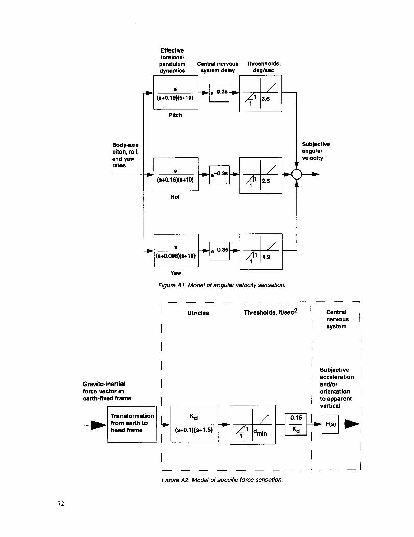
Body-axispitch, roll,and yawrates

Effectivetorsional

pendulumdynamics

(s+0.19)(s+10)

Pitch

Central nervous

system delay

Threshholds,deglsec

1 3.6

(s+0.16)(s+10)

Roll

/_1 1 2.5

s+0.0 s+10)

Ysw

Figure A 1. Mode/of angular velocity sensation.

Subjectiveangularvelocity

Grevito-inertislforce vector in

earth-fixed frame

---_l Transformation

from earth to

head frame

m

I Utricles

I

I

I

I

I

(s+0.1)ls+1.51

I

m --

Thresholds, ft/sec 2 Central

nervous

system

Subjectiveacceleration

and/ororientation

to apparent

vertical

II

IFigure A2. Model of specific force sensation.

?2

Head

roll

inertia

specific

torque(disturbance)

Desired

head

roll Muscle

__ 1330(s+12.5)

Head

1

s2+10s+7.812

73.8

Muscle spindle feedback

Specific torque

due to gravity

5(S+4)

(S+20)

Head

roll

Figure A3. Lateral head motion control model

F

Central nervousBody/pressure dynamics

system delay

0.036

_ e "0-05s

(s2+30s+1170)

Adaptation

ss+l

Figure A4. Body-pressure sensing model.

Offset threshold

/1

73

Appendix B--Height Regulation

Analysis with Previous Model

To acquire insight into the potential effects of motion on

a pilot during the performance of a task, a state-of-the-art

analytical model was used. The model was applied to the

experiment described under Vertical Experiment I (sec. 4).The task in that experiment was an altitude reposition

during hover, so it was a single-axis task. A plausibleinterconnection of the relevant system dynamics in the

task is shown in figure B 1. Here the pilot desires to attain

the commanded altitude, he. Based on the motion and

visual cues, the pilot then adjusts his collective control

position _i¢to zero the difference between his actual andcommanded altitude. All of the elements and connections

in figure B 1 are adequately known except for the pilotelement.

Aircraft

"e

'I tMo,,o -- system

t Visual Isystem _'_

Figure B1. Altitude reposition block diagram in simulation.

In particular, what is not known is how the pilot usesthe motion and visual cues to estimate vehicle state.

Although the motion system has only acceleration as its

input, and the visual system has only position as its

input, what are each of these system's effective outputs? Itis reasonable to assume that the motion system provides a

salient acceleration cue and that the visual system provides

a strong position cue. It is often assumed that the visual

system also supplies the velocity cue via the time-rate-of-change of the displayed positions. And certainly at a

steady-state velocity, the motion system provides no cue.

These very assumptions are made by Hess and Malsbury

(ref. 61) as shown in their "structural model of the pilot,"

which is reproduced in figure B2 in the context of the

altitude repositioning task discussed in section 4.

The pilot is assumed to close loops around vertical

acceleration, vertical velocity, and vertical displacement.

In the model, the acceleration is derived solely from the

motion feedback; however, it might be argued thatacceleration could also be derived from the second time-

derivative of the displacement. In the acceleration feedback

path, two dynamical elements are shown. The first is a

high-pass motion filter, which attenuates motion at all

frequencies via K and at frequencies below to. Both of

these parameters are adjustable in a given simulation

facility based on the task demands and the facility's

motion displacement capability. The second dynamic

element is the motion-system servo hardware. Using the

frequency-response testing techniques developed by

Tischler and Cauffman (ref. 46), the simulator has

vertical-axis drive dynamics (approximately) of

fisim (S) (8)(26) 031)hco m (s +8)(s + 26)

The vehicle vertical velocity and displacement are derived

from the visual system, which is represented by an

83-msec time delay. Hess and Malsbury point out inreference 61 that the vertical velocity sensing assumption

affects the primary control loop, but that it is currently

not known how to select the appropriate division of the

vertical velocity estimation between the motion and visualcues, which is a motivation for Vertical Experiment III

described in section 6.

The pilot gains shown in figure B2 are selected based on a

set of adjustment rules proposed by Hess and Malsbury.

For these tasks, only the high-pass filter was changed, and

using the adjustment rules results in the change of three

variables Kfi, Kfi, and K h. The gain Ki_ is determined so

that the lowest damping ratio of any oscillatory roots in

the h(s) / hc (s) transfer function is at least 0.15. This

value of damping ratio is selected to represent a trade-off

between stability and high-frequency phase-lag reduction(ref. 70). In reference 70, Hess points out that requiring an

identical damping ratio of this loop for all configurations

reduces the sensitivity of the modeling procedure to the

particular value chosen.

Then, with the motion loop closed, Kfiis determined so

as not to violate the combination of a phase margin of 45 °

and a gain margin of 4 dB in the vertical velocity open-

loop hcue(S)/he(s). These values are selected by Hess to

achieve adequate stability margins for the vertical-velocity

loop. Again, Hess states that requiring all configurations

to have the same level of relative stability (same phase

and gain margin) reduces the sensitivity of the model to

the particular values chosen.

75

hc +

r

iI

Pilot

IlIIIL--.

Central nervous and

neuromuscular system Aircraft• K_ .. ..

)._ - _ -I KS .. I dynamics .. motion filter i

Ihsim I hfilt 2 I

, I, '1 I-L

hcue

r i

I II • -0"083a _ i

I II II I

I II J

Visual systemhardware

I 1

Motion

system

Figure B2. Structural pilot model for Vertical Experiment I (ref. 61).

Finally, the gain K h is chosen to have adequate frequency

separation between the altitude and vertical-velocity loopswhile maintaining good altitude-loop crossover charac-

teristics. A useful rule-of-thumb is to separate the altitude

and vertical-velocity crossover frequencies by a factor of 4

(ref. 71).

This pilot gain determination process was repeated for the

high-pass motion filter variations in Vertical

Experiment I. Although the motion filter gain, K, was

changed in that experiment, note that the adjustment rules

of the model do not account for an effect due to that gain

K. That is because any changes in K are offset by adjust-

ments in Ki_. So, the model only predicts performancedifferences owing to changes in the motion-filter natural

frequency and not its gain.

For the five motion configurations that encompassed the

motion-filter natural frequency changes, the predictionsof the model are shown in table B 1. The motion-filter

configurations, V1, V2, V3, V4, and V10 are fully

described in Vertical Experiment I; however, V 1 essen-

tially represents a motion-filter transfer function of unity,

and V2 through V4 represent increasing break frequencies

of 0.245 to 0.885 tad/see. The V10 configuration has nomotion at all.

The last two columns of table B1 are the altitude-rate

pilot-vehicle crossover frequency and the closed-loop

altitude-rate bandwidth, respectively. The definition of

bandwidth used in reference 61 was that of the -90 ° phase

point. The frequency responses along with the bandwidth

measure are shown in figure B3.

Note that the analytical model predicts a reduction in the

vertical-velocity closed-loop bandwidth, from 6.36 to

4.27 rad/sec, as the motion feedback degrades from nearfull-motion to no motion. For the no-motion case, VI0,

the pilot has to increase his visual velocity feedback,

which results in a higher crossover frequency than before,

but in a lower closed-loop bandwidth.

76

TableB1.Analyticalpilot-vehiclecharacteristics.

Configuration Kh KI_ Ki_ lacue/ he toe(l/see) (1/sec) (rad/sec)

ia/lac BW(md/sec)

V1 0.323 0.542 0.217 1.20 6.36

V2 0.299 0.565 0.240 1.24 6.24

V3 0.335 0.595 0.215 1.33 6.13

V4 0.385 0.636 0.213 1.50 5.85

V10 0.795 0.725 0.000 3.10 4.27

2O

In"ID

"o

t-

10

-10

-20-1

10

n a I I I I I I I a I L a _ u I

10 01

10

-50

qD

- 1 O0

o.

-150

-200

10 °1

-- Vl

V2

.... V3

V4

VIO

%

t _ _ f , I

t i a L

10 0

Frequency, rad/sec

\

h L i

Figure B3. Closed-loop vertical-velocity frequency responses.

101

If the changes in the closed-loop system roots areexamined for the above configurations, the effective heave

damping goes from -1.4 sec 1 for the full-motion case(V1) to -1.1 sec I for the V4 configuration. The locationof this root accounts for much of the bandwidth difference.

This root is also the principal root of interest in the

pilot's control of altitude. The corresponding effects on

the other roots are minimal. The heave damping

argument, however, does not hold for the no-motion case(V10). In fact, although the bandwidth is less in this case,

the damping of the primary closed-loop roots is good.

The above model also predicts a degradation in closed-loop

performance from degradations in the motion filter alone.

77

FigureB4illustrateshowtheclosed-loop vertical-velocity

roots migrate as the motion filter changes. However, these

closed-loop poles are those that result when the model's

gains are fixed at the full-motion (V1) condition for all the

remaining conditions (V2, V3, V4, VI0). This situationwas examined to show the effect of the motion filter alone

without pilot adaptation. Only the region near the origin

is depicted, since the poles and zeros far from the origin

exhibit negligible change.

Two effects of the motion filter alone are noticed. First,

the effective heave damping is reduced as the motion

filter's natural frequency increases. This result also occurs

when the adjustment rules of the model are followed.

Second, pole-zero dipoles form in which the separation

between the pole and zero become more prominent as themotion filter is made more restrictive (going from VI to

V4). As the filter natural frequency increases, these dipoles

encroach upon the pilot-vehicle crossover frequency. Thus,

a broad range of integrator-like characteristics in the

crossover region does not occur. So if the pilot wanted to

achieve a similar, but slower, closed-loop response, more

than just a simple gain change on his part would be

necessary. He would also have to adjust his dynamic

compensation, which would likely entail an increase in

workload or a reduction in his opinion of simulator

fidelity. As expected, the closed-loop bandwidth without

using the pilot adjustment rules becomes worse. The

bandwidth of the VI0 configuration is 3.60 rad/sec

without the adjustment rules versus 4.27 rad/secwith them.

Since this model was applied to Vertical Experiment I

(sec. 4), it is interesting to compare the phase-plane time-histories from that experiment (figs. 40-43, 49) with the

phase-plane time-histories that the model predicts. The

model's predictions for the five configurations analyzed(V1, V2, V3, V4, and V10) are shown in figure B5.

Although the model shows degradations as the quality of

the platform motion becomes worse, the model poorly

represents the experimental results in two ways. First, the

model introduces a pronounced underdamped oscillatory

m

Nm

CI)Q

g

0.8

0.6

0.4

0.2

4}.2

4}.4

-0.6

-0.8

-1-2

I I I I I I I f I_ I

// × /v4

/ // /

/ // /

/ _' V3I o/ I \

IxlI I

kl

Decreasingheavedamping

..... X .... X..... XX .........

Vl V2 V3 V4

o

x

o

V2/_.

\jI v

x

I I i I J I I I i

-1.8 -1.6 -1.4 -1.2 -1 -0.8 -0.6 4}.4 -0.2Realaxis

Figure B4. Closed-loop vertical-velocity spectrum versus motion filter changes.

78

mode for the V1-V4 configurations, which has a frequency

of 8 rad/sec. This mode is not present in the experimental

results, which show a reasonably smooth response during

the ascent. Second, the model does not predict the oscilla-

tory behavior that occurs experimentally at the terminal

altitude point (85 ft), which is especially prevalent in the

motionless (V 10) configuration. The adjustment rules

need to be modified in the model in an attempt to match

the experimental results. This modification is left forfuture work.

It should be clear that some key assumptions are made in

the development of this model, such as which parts of the

simulator system provide which cues, and the adjustment

rules are somewhat of an art. The bottom line is that

today's models are incomplete and certainly not validated.

The lack of adequate analytical models has been noted by

others. Breuhaus pointed out that it is a dubious assump-

tion that one knows all of the important cues and their

interrelationships (ref. 72). Heffley et al. stated that when

a modeler begins to assemble all of the components that

are believed to influence the pilot-vehicle loop in simula-

tion that one notices the fragmentary nature of, and the

serious gaps in, the quantification of the componentcharacteristics (ref. 73). More empirical results from

systematic and realistic investigations are needed before

useful analytical models can be created.

12 I I I I I I I I I

10

8 ••

2

8

-2-10

6

"o

<4

I L

-8 -6

\

I I I L

-4 -2 0 2


Figure B5. Predicted phase-plane responses.

-- V1V2

- - V3

V4

• • V18

o

I I I

4 6 8 10

79

Appendix CmExample of

Repeated-Measures Analysis

A researcher wants to know if the differences among

collected data are due to a manipulated experimental factor,

or if they are due to random effects. If data are taken from

a random sample of individuals, each of whom has

experienced a different combination of the experimentalfactors, then experimental error may be attributed to two

effects. The first effect is sampling error and the second

effect is error resulting from differences among theindividuals.

Repeated-measures allows the differences amongindividuals to be accounted for in the analysis. This is

accomplished by having each individual experience each

experimental manipulation. It is a technique often used

when subjects are available for a long period of time, suchas in a research institution. Details of repeated-measures

theory may be found in Myers (ref. 54). Only a briefoverview will be given here. An example of the data

processing involved is given next.

The example uses the pilot compensation ratings forTask 1 in section 3 (15 ° yaw rotational capture). A plot

of the data is given in figure 15. Table C1 contains the

average compensation rating given by each pilot for all ofthe combinations of translational and rotational motion.

The first column gives the pilot number, 1-6. The second

column indicates if translational motion was present. A

l means translational motion was present, and a zeromeans it was not. Column three indicates if rotational

motion was present. Column four gives the average

compensation rating, where the average is taken over the

repeated runs performed by each pilot. Here the values

correspond to 0 = minimal, l = moderate, 2 = consid-erable, and 3 = maximum tolerable.

The purpose of the statistical analysis is to determine if

pilots provide better compensation ratings for particular

motion configurations. Specifically, it can be determined

if the ratings are influenced by the presence of transla-

tional motion, by the rotational motion, or by a combi-

nation of the two motions. Although figure 15 suggests

that the translational motion is likely to be the dominant

factor, the statistical analysis provides quantitativeinformation on how often such variations are due to

random effects. So, the analysis indicates how solid theinferences drawn from the data are.

Table C 1. Average pilot compensation ratings for yaw

experiment Task 1.

Pilot (i) Translational Rotational Average

on (j) on (k) rating (Y)

1 0 0 2.67

1 0 1 2.25

1 1 0 1.75

1 1 1 1.75

2 0 0 2.25

2 0 1 1.75

2 1 0 0.75

2 1 1 0.00

3 0 0 1.25

3 0 1 1.25

3 1 0 1.00

3 l 1 1.00

4 0 0 3.00

4 0 1 3.00

4 1 0 3.00

4 1 1 3.00

5 0 0 2.50

5 0 1 2.50

5 1 0 0.25

5 1 1 0.00

6 0 0 1.75

6 0 1 2.00

6 1 0 1.25

6 1 1 1.00

To determine whether the differences noted owing to

translational motion are statistically significant, the ratio

MStran s / MSuan_lpil.t is formed. The numerator of this ratio,MS_,s is the between-groups mean square. The denomi-

nator of this ratio, MStrans/pilo t, is the population errorvariance. The higher this ratio, the more likely that the

differences between the two translational configurationsare due to the effect of translational motion and that they

are not random results. The relations for these terms are:

F - MStrans (CI)

MStrans / pilot

MStran s - SStrans (C2)(a-l)

81

where

SStrans / pilot

MSwans/pil°t - (a - l)(n - 1)

SStrans/pilot -

Ik _ Yijk ]2

SSu_ls -

- C - SStran s - SSpilo t

nb

and for Task 1 in the Yaw experiment:

SSpil°t = ab

E Yijk

C= J

i = 1..... 6 = pilot

abn

C

C

j = 0,1 = translational configuration (off or on)

k = 0,1 = rotational configuration (off or on)

a = 2 = number of lateral configurations

b = 2 = number of rotational configurations

n = 6 = number of pilots

Using the values from table C1, then the equations_,come

C - (40'92)2 = 69.77(2)(2)(6)

(8.42) 2 + (4.75) 2 + (4.50) 2

+ (12.00) 2 + (5.25) 2 + (6.00) 2

SSpil°t = (2)(2)

- 69.77 = 10.55

(C3)

(C4)

(C5)

(C6)

(C7)

(C8)

(C9)

SStran s =

SStrans/pilo t =

(26"17)2 +(14"75)2 69.77= 5.43 (CIO)(6)(2)

-(4.92) 2 + (4.00) 2 + (2.50) 2

+ (6.00) 2 + (5.00) 2 + (3.75) 2

2

"(3.50) 2 + (0.75) 2 + (2.00) 2

+ (6.00) 2 + (0.25) 2 + (2.25) 24- (CI1)

2

- 69.77 - 5.43 - 10.55 = 3.98

3.98MStrans/pilo t - - 0.796 (C12)

(1)(5)

5.43MStran s - - 5.43 (C13)

(1)

5.43F - = 6.82 (C14)

0.796

Statistically, the F-ratio is the distribution of the ratio of

two independently distributed chi-squares each divided by

their degrees of freedom. The degrees of freedom are the

number of independent observations that were summed in

obtaining the chi-square distribution. For the above

F-ratio example, the numerator and denominator have

(a - 1 = 1) and (n - 1 = 5) degrees of freedom, respec-

tively. The resulting F-ratio, for these degrees-of-freedom,

is then be compared against tabulated critical regions to

determine if it is large enough to be considered significant.

If the F-ratio is large enough, then the effect of the

experimental factor is said to be significant. Otherwise,

the differences may be due to random error. In the

example, an F = 6.82 means there are 4.7 chances in 100

that the differences would occur randomly. These low odds

suggest that turning translational motion on and off is

affecting the results.

82

Appendix DmReview of Cooper-

Harper Handling Qualities RatingScale

The term "handling qualities" is defined as "those qualities

or characteristics of an aircraft that govern the ease and

precision with which a pilot is able to perform the tasks

required in support of an aircraft role" (ref. 53). The

subjective scale that has become the worldwide standard

for measuring handling qualities is the Cooper-Harper

Handling Qualities Rating Scale (ref. 53), which is shown

in figure D1.

After completing a flying task, the pilot assigns a

numerical rating by proceeding through the decision treeon the left-hand side of the scale. The decision tree

separates the handling qualities into four categories:

(1) satisfactory (rating<3.5), (2) unsatisfactory but

tolerable (3.5 < rating < 6.5), (3) unacceptable (6.5 <

rating < 9.5), and (4) uncontrollable (9.5 < rating). The

first three categories are referred to as Level 1, Level 2,

and Level 3 handling qualities, respectively.

The first question, "Is it controllable?," must be answered

in the context of the task. If the pilot can control the

aircraft in order to perform the task, even if it requires hisundivided attention, then the aircraft is controllable.

Otherwise, the aircraft is uncontrollable, and the assigned

rating is a 10.

The second question, "Is adequate performance attainable

with a tolerable pilot workload?," requires the experi-

menter to define performance standards. Engineers and

pilots, at the beginning of an experiment, jointly decide

on two performance standards: desired and adequate. An

example would be for a pilot to fly a landing approachwhile maintaining airspeed to within +5 knots for desired

performance and +10 knots for adequate performance.

Returning to the second question, the pilot nowdetermines not only whether the adequate performance

standard was met, but if the workload was also tolerable.

If the answer to this question is yes, then the task can be

performed with reasonable precision, even though it mighttake considerable mental and physical compensation on

the part of the pilot.

If the pilot proceeds to the third question, "Is it

satisfactory without improvement?" he now has to decide

whether the vehicle is good enough as it is for its intendeduse or if he thinks it should be changed. The vehicle does

not have to be perfect, just good enough.

When the pilot proceeds to the right-hand side of the scale,

a numerical rating is assigned based on the descriptors ofthe aircraft characteristics and the demands on the pilot.

This process is often a balance between the performance

achieved and the compensation required by the pilot in

order to achieve that performance.

The Cooper-Harper Handling Qualities Scale has been

used successfully since 1969, and it is an excellent way to

obtain high-quality subjective data from pilots. These dataoften correlate well with the objective data collected.

83

Adequacy for Selected Task orRequired Operation*

I Yes

Is itsatisfactory without

improvement?

TYes

Is adequateperformance No

attainable with a tolerablepilot workload?

_Yes

is Noit controllable?

Start

No Deficiencies--_ warrant

improvement

AircraftCharacteristics

ExcellentHighly desirable

GoodNegligible deficiencies

Fair - Some mildlyunpleasant deficiencies

Demands on the Pilot in Selected HQRTask or Required Operation*

Pilot compensation not a factor for 1desired performance

Pilot compensation not a factor for 2desired performance

Minimal pilot compensation required fordesired performance 3

Deficienciesrequire

improvement

Minor but annoyingdeficiencies

Moderately objectionabledeficiencies

Very objectionable buttolerable deficiencies

Major deficiencies

Major deficiencies

Major deficiencies

Improvementv mandatory _ Major deficiencies

Desired performance requires moderatepilot compensation

Adequate performance requiresconsiderable pilot compensation

Adequate performance requires extensive 6pilot compensation

Adequate performance not attainable withmaximum tolerable pilot compensation.Controllability not in question.

Considerable pilot compensation is required 8for control

Intense pilot compensation is required to 9retain control

Control will be lost during someportion of required operation

*Definition of required operation involves designation of flightphase and subphases with accompanying conditions.

10

Figure D1. Cooper-Harper Handling Qualities Rating Scale.

84

References

1. Haward, D. M.: The Sanders Teacher. Flight, vol. 2,

no. 50, Dec. 1910, pp. 1006-1007.

2. Baarspul, M.: A Review of Flight Simulation

Techniques. Progress in Aerospace Sciences, vol. 27,

1990, pp. 1-120.

3. Airplane Simulator Qualification. FAA Advisory

Circular AC 120-40B, U. S. Department of

Transportation, Washington, D. C., July 1991.

4. Donohue, J. A.: Keepin' the Shiny Side Up. Air

Transport World, vol. 32, no. 10, Oct. 1995,

pp. 47-50.

5. Helicopter Simulator Qualification. FAA Advisory

Circular AC- 120-63, U. S. Department of Transpor-

tation, Washington, D. C., Oct. 1994.

6. Johnston, D. E.; and McRuer, D. T.: Investigation of

Interactions between Limb-Manipulator Dynamicsand Effective Vehicle Roll Control Characteristics.

NASA CR-3983, 1986.

7. Watson, D. C.; and Schroeder, J. A.: Effects of Stick

Dynamics on Helicopter Flying Qualities. AIAA

Paper 90-3477, Proceedings of the AIAA Guidance,

Navigation, and Control Conference, Portland, Oreg.,

1990, pp. 1460-1479.

8. Boldovici, J. A.: Simulator Motion. U. S. Army

Research Institute Technical Report 961, Alexandria,

Va., Sept. 1992.

9. Cardullo, F. M.: An Assessment of the Importance of

Motion Cuing Based on the Relationship Between

Simulated Aircraft Dynamics and Pilot Performance:

A Review of the Literature. Paper No. 91-2980,

Proceedings of the AIAA Flight Simulation Tech-

nologies Conference, New Orleans, La., 1991,

pp. 436-447.

10. Roscoe, S. N.: Aviation Psychology. The Iowa State

University Press, Ames, Iowa, 1980.

11. Waters, B. K.; Grunzke, P. M.; Irish, P. A., III; and

Fuller, J. H., Jr.: Preliminary Investigation of

Motion, Visual, and g-Seat Effects in the Advanced

Simulator for Undergraduate Pilot Training (ASUPT).

Proceedings of the AIAA Visual and MotionSimulation Conference, 1976.

12. Gray, T. H.; and Fuller, R. R.: Effects of Simulator

Training and Platform Motion on Air-to-Surface

Weapons Delivery Training. AFHRL TR-77-29,

July 1977.

13. Simulator Sickness Field Manual Mod. 3. U. S.

Naval Training Systems Center, Orlando, Fla., 1988.

14. Hunter, S.; Gundry, A. J.; and Rolfe, J. M.: Human

Factors in Flight Simulation: Annotated Bibliog-

raphy. AGARD Report R-656, 1977.

15. Puig, J. A.; Harris, W. T.; and Ricard, G. L.: Motion

in Flight Simulation: An Annotated Bibliography.

NAVTRAEQUIPC-IH-298, Naval Training

Equipment Center, Orlando, Fla., 1978.

16. Hall, J. R.: The Need for Platform Motion in Modern

Piloted Flight Training Simulators. Technical

Memorandum FM35, The Royal Aerospace

Establishment, Bedford, U. K., Oct. 1989.

17. Showalter, T. W.; and Parris, B. L.: The Effects of

Motion and g-Seat Cues on Pilot Simulator

Performance of Three Piloting Tasks. NASA

TP-1601, 1980.

18. Young, L. R.: Some Effects of Motion Cues onManual Tracking. AIAA J. Spacecraft and Rockets,

vol. 4, no. 10, 1967, pp. 1300-1303.

19. Hosman, R. J. A. W.; and van der Vaart, J. C.:

Thresholds of Motion Perception and Parameters ofVestibular Models Obtained from Tests in a Motion

Simulator: Effects of Vestibular and Visual Motion

Performance on Task Performance. Memorandum

M-372, Delft University of Technology, Delft,

Netherlands, 1980.

20. McMillan, G. R.; Martin, E. A.; Flach, J. M.; and

Riccio, G. E.: Advanced Dynamic Seat: An

Alternative to Platform Motion. Proceedings of the

7th Interservice/Industry Training Equipment

Conference, Nov. 1985, pp. 153-163.

21. Levison, W. H.; Lancraft, R. E.; and Junker, A. M.:

Effects of Simulator Delays on Performance and

Learning in a Roll Axis Tracking Task. AFFDL

TR-3134, Wright-Patterson Air Force Base, Ohio,

1979, pp. 168-188.

22. Meiry, J. L.: The Vestibular System and Human

Dynamic Space Orientation. NASA CR-628, 1966.

23. Shirley, R. S.; and Young, L. R.: Motion Cues inMan-Vehicle Control. IEEE Trans. on Man-Machine

Sys., vol. MMS-9, no. 4, 1968, pp. 121-128.

24. Bray, R. S.: Visual and Motion Cueing in HelicopterSimulation. NASA TM-86818, 1985.

25. Rolfe, J. M.; and Staples, K. J.: Flight Simulation.

Cambridge University Press, Cambridge, 1986,

p. 117.

85

26.Stapleford,R.L.;Peters,R.A.;andAlex,F.R.:ExperimentsandaModelforPilotDynamicswithVisualandMotionInputs.NASACR-1325,1969.

27.Bray,R.S.:InitialOperatingExperiencewithanAircraftSimulatorHavingExtensiveLateralMotion.NASATMX-62155,May1972.

28.Peters,R.A.:DynamicsoftheVestibularSystemandTheirRelationtoMotion Perception, Spatial

Disorientation, and Illusions. NASA CR-1309,

Apr. 1969.

29. Young, L. R.; Meiry, J. L.; Newman, J. S.; and

Feather, J. E.: Research in Design and Development

of a Functional Model of the Human Nonauditory

Labyrinths. AMRL TR-68-102, Dayton, Ohio, 1969.

30. Gum, D. R.: Modeling of the Human Force and

Motion-Sensing Mechanisms. AFHRL TR-72-54,

Wright-Patterson Air Force Base, Ohio, June 1973.

31. Zacharias, G. L.: Motion Cue Models for Pilot-

Vehicle Analysis. AMRL TR-78-2, Wright-PattersonAir Force Base, Ohio, Mar. 1978.

32. Van Egmond, A. A. J.; Groen, J. J.; and Jongkees,L. B. W.: The Mechanics of Semicircular Canal.

J. Physiol., vol. 110, 1949, pp. 1-17.

33. Jones, G. M.; Barry, W.; and Kowalsky, N.:

Dynamics of Semicircular Canals Compared in Yaw,

Pitch, and Roll. Aerospace Medicine, vol. 35,

no. 10, 1964, pp. 984-989.

34. Young, L. R.; and Oman, C. M.: Model for

Vestibular Adaptation to Horizontal Rotation.

Aerospace Medicine, vol. 40, no. 10, 1969,

pp. 1076-1080.

35. Levison, W. H; and Junker, A. M.: A Model for the

Pilot's Use of Motion Cues in Roll-Axis Tracking

Task. Bolt, Beranek, and Newman Report No. 3528,June 1977.

36. Samji, A.; and Reid, L. D.: The Detection of Low

Amplitude Yawing Motion Transients in a Flight

Simulator. IEEE Trans. Systems, Man, and

Cybernetics, vol. 22, no. 2, Mar./Apr. 1992,

pp. 300-306.

37. McRuer, D. T.; and Krendel, E. S.: Mathematical

Models of Human Pilot Behavior. AGARDograph

No. 188, Jan. 1974.

38. Bergeron, H. P.: The Effects of Motion Cues on

Compensatory Tasks. AIAA Paper 70-352, 1970.

39. van Gool, M. F. C.: Influence of Motion Washout

Filters on Pilot Tracking Performance. Paper 19,

AGARD-CP-249, 1978.

40. Cooper, D. E.; and Howlett, J. J.: Ground Based

Helicopter Simulation. American Helicopter Society

Symposium on Status of Testing and Model

Techniques for V/STOL Aircraft, Esssington, Pa.,1973.

41. Jex, H. R.; Magdaleno, R. E.; and Junker, A. M.:

Roll Tracking Effects of g-Vector Tilt and Various

Types of Motion Washout. NASA CP-2060, 1978,

pp. 463-502.

42. Shirachi, D. K.; and Shirley, R. S.: Visual/MotionCue Mismatch in a Coordinated Roll Maneuver.

NASA CR-166259, Nov. 1981.

43. Jex, H. R.; Jewell, W. F.; Magdaleno, R. E.; and

Junker, A. M.: Effects of Various Lateral-Beam

Washouts on Pilot Tracking and Opinion in the

Lamar Simulator. AFFDL-TR-79-3134, 1979,

Dayton, Ohio, pp. 244-266.

44. Sinacori, J. B.: The Determination of Some

Requirements for a Helicopter Flight Research

Simulation Facility. NASA CR-152066, 1977.

45. Danek, G. L.: Vertical Motion SimulatorFamiliarization Guide. NASA TM-103923, 1993.

46. Tischler, M. B.; and Cauffman, M. G.: Frequency-

Response Method for Rotorcraft System Identifi-

cation: Flight Applications to BO-105 Coupled

Rotor/Fuselage Dynamics. J. Am. Helicop. Soc.,

vol. 37, no. 3, July 1992, pp. 3-17.

47. Mitchell, D. G.; and Hart, D. C.: Effects of

Simulator Motion and Visual Characteristics on

Rotorcraft Handling Qualities Evaluations. NASA

CR-3220, 1993, pp. 341-359.

48. Schroeder, J. A.: Simulation Motion Effects on

Single Axis Compensatory Tracking. Paper

No. 93-3579, Proceedings of AIAA Flight

Simulation Technologies Conference, Monterey,

Calif., Aug 1993, pp. 202-213.

49. Schroeder, J. A.: Evaluation of Simulation Motion

Fidelity Criteria in the Vertical and Directional Axes.

J. Am. Helicop. Soc., vol. 41, no. 2, Apr. 1996,

pp. 44-57.

50. Handling Qualities Requirements for Military

Rotorcraft. Aeronautical Design Standard 33D

(ADS-33D), U. S. Army Aviation and Troop

Command, St. Louis, Mo., July, 1994.

86

51.Schroeder,J.A.;Tischler,M.B.;Watson,D.C.;andEshow,M.M.;IdentificationandSimulationEvaluationofaCombatHelicopterinHover.AIAAJ.Guidance,Control,andDynamics,vol.18,no.1,1995,pp.31-38.

52.McFarland,R.E.:TransportDelayCompensationforComputer-GeneratedImagerySystems.NASATM-100084,1988.

53.Cooper,G.E.;andHarper,R.P.,Jr.:TheUseofPilotRatingin theEvaluationofAircraftHandlingQualifies.NASATND-5153,1969.

54.Myers,J.L.:FundamentalsofExperimentalDesign.AllynandBacon,Inc.,Boston,1972,pp.167-190.

55.Young,L. R.:VisuallyInducedMotioninFlightSimulation.Paper16,AGARDCP-249,Brussels,1978.

56.Zacharias,G.L.;andYoung,L.R.:InfluenceofCombinedVisualandVestibularCuesonHumanPerceptionandControlofHorizontalRotation.ExperimentalBrainResearch,vol.41,no.2,pp.159-171.

57.Schroeder,J.A.;Moralez,E.;andMerrick,V.K.:SimulationEvaluationoftheControlSystemCommandMonitoringConceptfortheNASAV/STOLResearchAircraft(VSRA).AIAAPaper87-2255,ProceedingsofAIAAGuidance,NavigationandControlConference,Monterey,Calif.,Aug.1987,pp.133-154.

58.Heffley,R.K.;Jewell,W.F.;Lehman,J.M.;andVanWinkle,R.A.:A CompilationandAnalysisofHelicopterHandlingQualitiesData.Vol.1:DataCompilation. NASA CR-3144, 1979.

59. Schroeder, J. A.; Tischler, M. B.; Watson, D. C.;

and Eshow, M. M.: Identification and Simulation

Evaluation of an AH-64 Helicopter Hover Math

Model. Paper No. 91-2877, Proceedings of the

AIAA Atmospheric Flight Mechanics Conference,New Orleans, La., 1991, pp. 264-297.

60. Bray, R. S.: A Study of Vertical Motion

Requirements for Landing Simulation. HumanFactors, vol. 15, no. 6, 1973, pp. 561-568.

61. Hess, R. A.; and Malsbury, T.: Closed-Loop

Assessment of Flight Simulator Fidelity. AIAA

J. Guidance, Control, and Dynamics, vol. 14,

no. 1, 1991, pp. 191-197.

62. Snedecor, G. W.; and Cochran, W. G.: Statistical

Methods, Sixth Ed., The Iowa State University Press.

Ames, Iowa, 1967, p. 265.

63. Paulk, C. H., Jr.; Astill, D. L.; and Donley, S. T.:Simulation and Evaluation of the SH-2F Helicopter

in a Shipboard Environment Using the Interchange-

able Cab System. NASA TM-84387, 1983.

64. Ferguson, S. W.; Clement, W. F.; Cleveland, W. B.;

and Key, D. L.: Assessment of Simulation Fidelity

Using Measurements of Piloting Technique in Flight.

Proceedings of the American Helicopter Society, May

1984, pp. 67-92.

65. Johnson, W. W.; and Schroeder, J. A.: Visual-

Motion Cueing in the Control of Altitude. IEEEInternational Conference on Systems, Man, and

Cybernetics, Vancouver, British Columbia, Oct.

1995, pp. 2676-2681.

66. Warren, R.: Optical Transformation during

Movement: Review of the Optical Concomitants of

Egomotion. Report No. AFOSR-TR-82-1028,

Aviation Psychology Laboratory, Ohio State

University, Columbus, Ohio, Oct. 1982.

67. Johnson, W. W.; and Awe, C. A.: The Selective Use

of Functional Optical Variables in the Control of

Forward Speed. NASA TM-108849, 1994.

68. Grant, P. R.; and Reid, L. D.: Motion Washout

Filter Tuning: Rules and Requirements. AIAA J.

Aircraft, vol. 34, no. 2, Mar.-Apr. 1997,

pp. 145-151.

69. Grant, P. R.; and Reid, L. D.: PROTEST: An Expert

System for Tuning Simulator Washout Filters.

AIAA J. Aircraft, vol. 34, no. 2, Mar.-Apr. 1997,

pp. 152-159.

70. Hess, R. A.: Model for Human Use of Motion Cuesin Vehicular Control. AIAA J. Guidance, Control,

and Dynamics, vol. 13, no. 3, 1990, pp. 476-482.

71. Hess, R. A.: Theory for Aircraft Handling Qualities

Based upon a Structural Pilot Model. AIAA J.Guidance, Control, and Dynamics, vol. 12, no. 6,

1989, pp. 792-797.

72. Breuhaus, W. O.: Recent Experience with In-Flight

Simulation., AGARD CP-17, pt. 2, Sept. 1966,

pp. 577-620.

73. Heffley, R. K.; Clement, W. F.; et al.: Determina-tion of Motion and Visual System Requirements for

Flight Training Simulators. Technical Report 546,

U. S. Army Research Institute for the Behavioral andSocial Sciences, Fort Rucker, Ala., Aug. 1981.

87

Form Approved

REPORT DOCUMENTATION PAGE OM8No.ozo4-ola8

Public reporting burden for this collection of information is estimated to average 1 hour per response, including the time for rewewing instructions, searching existing data sources,gathering and maintaimng the data needed, and completing and reviewing the collection of information Send comments regarding this burden estimate or any other aspect of thiscollection of information, including suggestions for reducing this burden, to Washington Headquarters Services, Directorate for information Operations and Reports, 1215 JeffersonDavis Highway, Suite 1204, Arlington, VA 22202-4302, and to the Office of Management and Budget, Paperwork Reduction Project (0704-0t88), Washington, DC 20503

I

1. AGENCY USE ONLY (Leave blank) 2. REPORT DATE 3. REPORT TYPE AND DATES COVERED

July 1999 Technical Publication4. TITLE AND SUBTITLE 5. FUNDING NUMBERS

Helicopter Flight Simulation Motion Platform Requirements

8. AUTHOR(S)

Jeffery Allyn Schroeder

7. PERFORMINGORGANIZATIONNAME(S)ANDADDRESS(ES)


Moffett Field, CA 94035-11300

9. SPONSORING/MONITORING AGENCY NAME(S) AND ADDRESS(ES)

National Aeronautics and Space Administration

Washington, DC 20546-0001

548-40-12

8. PERFORMING ORGANIZATION

REPORT NUMBER

A-9900432

10. SPONSORING/MONITORING

AGENCY REPORT NUMBER

NASA/TP-1999-208766

11. SUPPLEMENTARY NOTES

Point of Contact: Jeffery Allyn Schroeder, Ames Research Center, MS 262-2(650) 604-4037

Moffett Field, CA 94035-1000

12S. DISTRIBUTION/AVAILABILITY STATEMENT

Unclassified -- Unlimited

Subject Category O1

Availability: NASA CASI (301) 621-0390

Distribution: Standard

12b. DISTRIBUTION CODE

13. ABSTRACT (Maximum 200 words)

To determine motion fidelity requirements, a series of piloted simulations was performed. Several

key results were found. First, lateral and vertical translational platform cues had significant effects on fidelity.

Their presence improved performance and reduced pilot workload. Second, yaw and roll rotational platform

cues were not as important as the translational platform cues. In particular, the yaw rotational motion plat-

form cue did not appear at all useful in improving performance or reducing workload. Third, when the lateral

translational platform cue was combined with visual yaw rotational cues, pilots believed the platform was

rotating when it was not. Thus, simulator systems can be made more efficient by proper combination of

platform and visual cues. Fourth, motion fidelity specifications were revised that now provide simulator users

with a better prediction of motion fidelity based upon the frequency responses of their motion control laws.

Fifth, vertical platform motion affected pilot estimates of steady-state altitude during altitude repositionings.

Finally, the combined results led to a general method for configuring helicopter motion systems and for

developing simulator tasks that more likely represent actual flight. The overall results can serve as a guide to

future simulator designers and to today's operators.

14. SUBJECT TERMS

Flight simulation, Helicopters, Motion platforms

17. SECURITY CLASSIFICATION

OF REPORT

Unclassified

NSN 7540-01-280-5500


OF THIS PAGE

Unclassified


OF ABSTRACT

15. NUMBER OF PAGES

8416. PRICE CODE

A05

20. LIMITATION OF ABSTRACT

Standard Form 298 (Rev 2-89)Prescribed by ANSI Std Z39-lS

2ge- 102

helicopter flight simulation motion platform requirements · · 2013-08-30helicopter flight...

Documents