helical waveguide with two bendings, and applications …

Progress In Electromagnetics Research B, Vol. 26, 115–147, 2010

HELICAL WAVEGUIDE WITH TWO BENDINGS, ANDAPPLICATIONS

Z. Menachem and S. Tapuchi

Department of Electrical EngineeringSami Shamoon College of EngineeringIsrael

Abstract—This paper presents an improved approach for thepropagation of electromagnetic (EM) fields along a helical hollowwaveguide that consists of two bendings in the same direction. Inthis case, the objective is to develop a mode model for infrared (IR)wave propagation, in order to represent the effect of the radius of thecylinder of the helix and the step’s angle on the output fields and theoutput power transmission. This model enables us to understand moreprecisely the influence of the step’s angle and the radius of the cylinderof the helix on the output results of each section (bending). The outputtransverse components of the field, the output power transmission andthe output power density for all bending are improved by increasingthe step’s angle or the radius of the cylinder of the helix, especially inthe cases of space curved waveguides. This mode model can be a usefultool to improve the output results in all the cases of the helical hollowwaveguides with two bendings for industrial and medical regimes.

1. INTRODUCTION

Various methods of cylindrical hollow metallic or metallic with innerdielectric coating waveguide have been proposed in the literature [1–18]. A review of the hollow waveguide technology [1, 2] and areview of IR transmitting, hollow waveguides, fibers and integratedoptics [3] were published. The first theoretical analysis of the problemof hollow cylindrical bent waveguides was published by Marcatiliand Schmeltzer [4], where the theory considers the bending as asmall disturbance and uses cylindrical coordinates to solve Maxwell

Received 15 August 2010, Accepted 19 September 2010, Scheduled 29 September 2010Corresponding author: Z. Menachem ([email protected]).

116 Menachem and Tapuchi

equations. They derive the mode equations of the disturbed waveguideusing the ratio of the inner radius r to the curvature radius R as a smallparameter (r/R ¿ 1). Their theory predicts that the bending has littleinfluence on the attenuation of a hollow metallic waveguide. However,practical experiments have shown a large increase in the attenuation,even for a rather large R.

Marhic [5] proposed a mode-coupling analysis of the bendinglosses of circular metallic waveguide in the IR range for large bendingradii. In the circular guide it is found that the preferred TE01 modecan couple very effectively to the lossier TM11 mode when the guideundergoes a circular bend. The mode-coupling analysis [5] developedto study bending losses in microwave guides has been applied to IRmetallic waveguides at λ = 10.6µm. For circular waveguides, themicrowave approximation has been used for the index of refraction andthe straight guide losses, and the results indicate very poor bendingproperties due to the near degeneracy of the TE01 and TM11 modes,thereby offering an explanation for the high losses observed in practice.

Miyagi et al. [6] suggested an improved solution, which providedagreement with the experimental results, but only for r/R ¿ 1. Adifferent approach [5, 7] treats the bending as a perturbation thatcouples the modes of a straight waveguide. That theory explainsthe large difference between the metallic and metallic-dielectric bentwaveguide attenuation. The reason for this difference is that in metallicwaveguides the coupling between the TE and TM modes caused by thebending mixes modes with very low attenuation and modes with veryhigh attenuation, whereas in metallic-dielectric waveguides, both theTE and TM modes have low attenuation. The EH and HE modes havesimilar properties and can be related to modes that have a large TMcomponent.

Hollow waveguides with both metallic and dielectric internallayers were proposed to reduce the transmission losses. Hollow-corewaveguides have two possibilities. The inner core materials haverefractive indices greater than one (namely, leaky waveguides) or theinner wall material has a refractive index of less than one. A hollowwaveguide can be made, in principle, from any flexible or rigid tube(plastic, glass, metal, etc.) if its inner hollow surface (the core) iscovered by a metallic layer and a dielectric overlayer. This layerstructure enables us to transmit both the TE and TM polarizationwith low attenuation [5, 7].

A method for the EM analysis of bent waveguides [8] is based onthe expansion of the bend mode in modes of the straight waveguides,including the modes under the cutoff. A different approach to calculatethe bending losses in curved dielectric waveguides [9] is based on

Progress In Electromagnetics Research B, Vol. 26, 2010 117

the well-known conformal transformation of the index profile andon vectorial eigenmode expansion combined with perfectly matchedlayer boundary conditions to accurately model radiation losses. Animproved ray model for simulating the transmission of laser radiationthrough a metallic or metallic dielectric multibent hollow cylindricalwaveguide was proposed in [10, 11]. It was shown theoretically andproved experimentally that the transmission of CO2 laser radiation ispossible even through bent waveguide.

The propagation of EM waves in a loss-free inhomogeneous hollowconducting waveguide with a circular cross section and uniform planecurvature of the longitudinal axis was considered in [12]. For smallcurvature the field equations can be solved by means of an analyticalapproximation method. In this approximation the curvature of theaxis of the waveguide was considered as a disturbance of the straightcircular cylinder, and the perturbed torus field was expanded ineigenfunctions of the unperturbed problem. An extensive survey of therelated literature can be found especially in the book on EM waves andcurved structures [13]. The radiation from curved open structures ismainly considered by using a perturbation approach, that is by treatingthe curvature as a small perturbation of the straight configuration.The perturbative approach is not entirely suitable for the analysis ofrelatively sharp bends, such as those required in integrated optics andespecially short millimeter waves.

The models based on the perturbation theory consider the bendingas a perturbation (r/R ¿ 1), and solve problems only for a large radiusof curvature.

Several methods of propagation along the toroidal and helicalwaveguides were developed in [14–18], where the derivation is basedon Maxwell’s equations. The method in [14] has been derived forthe analysis of EM wave propagation in dielectric waveguides witharbitrary profiles, with rectangular metal tubes, and along a curveddielectric waveguide. An improved approach has been derived for thepropagation of EM field along a toroidal dielectric waveguide with acircular cross-section [15]. The method in [16] has been derived forthe propagation of EM field along a helical dielectric waveguide witha circular cross section. The method in [17] has been derived for thepropagation of EM field along a helical dielectric waveguide with arectangular cross section. It is very interesting to compare betweenthe mode model methods for wave propagation in the waveguide witha rectangular cross section, as proposed in Refs. [14, 17] as regardto the mode model methods for wave propagation in the waveguidewith a circular cross section, as proposed in [15, 16]. The methodsin [14, 15] have been derived for one bending of the toroidal waveguide


(approximately a plane curve) in the case of small values of step angleof the helix. The methods in [16, 17] have been derived for one bendingof the helical waveguide (a space curved waveguide) for an arbitraryvalue of the step’s angle of the helix. The method in [18] has beenderived for the propagation of EM field along the toroidal waveguidethat consists of two bendings in the same direction, and the main stepsof the method for the two bendings were introduced, in detail, for smallvalues of step angles. The methods in [14–18] employ toroidal or helicalcoordinates (and not cylindrical coordinates, such as in the methodsthat considered the bending as a perturbation (r/R ¿ 1)).

The calculations in all the two above methods [14–18], are basedon using Laplace and Fourier transforms, and the output fields arecomputed by the inverse Laplace and Fourier transforms. Laplacetransform on the differential wave equations is needed to obtain thewave equations (and thus also the output fields) that are expresseddirectly as functions of the transmitted fields at the entrance of thewaveguide at ζ = 0+. Thus, the Laplace transform is necessary toobtain the comfortable and simple input-output connections of thefields. The objective in all these methods [14–18] was to develop amode model in order to provide a numerical tool for the calculation ofthe output fields for a curved waveguide. The technique of the methodsis quite different. The technique for a rectangular cross section [14, 17]is based on Fourier coefficients of the transverse dielectric profile andthose of the input wave profile, and the output fields were computedby the inverse Laplace and Fourier transforms. On the other hand,the technique for a circular cross section [15, 16, 18] was based onthe development of the longitudinal components of the fields intoFourier-Bessel series, and the transverse components of the fields wereexpressed as functions of the longitudinal components in the Laplaceplane and were obtained by using the inverse Laplace transform.

The main objective of this paper is to generalize the method [18]from a toroidal dielectric waveguide (approximately a plane curve) withtwo bendings to a helical waveguide (a space curved waveguide for anarbitrary value of the step’s angle of the helix) with two bendings.The objective is to presents an improved approach for the propagationof EM field in the case of the helical waveguide that consists of twobendings in the same direction. The main steps of the method forthe helical waveguide with two bendings will be introduced in thederivation, for arbitrary values of the step’s angle (and not for smallvalues of step angles). Our method employs helical coordinates (andnot cylindrical coordinates, such as in the methods that consideredthe bending as a perturbation (r/R ¿ 1)). The derivation for the firstsection and the second section of the helical waveguide with the two


bendings is based on Maxwell’s equations. The separation of variablesis obtained by using the orthogonal-relations. The longitudinalcomponents of the fields are developed into the Fourier-Bessel series.The transverse components of the fields are expressed as functions ofthe longitudinal components in the Laplace plane and are obtained byusing the inverse Laplace transform by the residue method. The resultsof this model are applied to the study of helical hollow waveguideswith two bendings, that are suitable for transmitting IR radiation,especially CO2 laser radiation. In this paper, we supposed that themodes excited at the input of the waveguide by the conventional CO2

laser IR radiation (λ = 10.6µm) are closer to the TEM polarizationof the laser radiation. The TEM00 mode is the fundamental and themost important mode. This means that a cross-section of the beamhas a Gaussian intensity distribution.

2. THE DERIVATION

The method presented in [18] is generalized from a toroidal waveguide(approximately a plane curve) with two bendings to a helical waveguide(a space curved waveguide for an arbitrary value of the step’s angle ofthe helix) with two bendings. Namely, the calculations in our methodare dependent also on the arbitrary value of the step’s angle of the helix.This model enables us to understand more precisely the influence of thestep’s angle and the radius of the cylinder of the helix on the outputresults of each section (bending).

(a) (b)

E = E , E = E ro2 r1 θo2 θ1

H = H , H = H ro2 r1 θo2 θ1

I

II

E , E r2 θ2

H , H r2 θ2

E , E ro θo

H , H ro θo

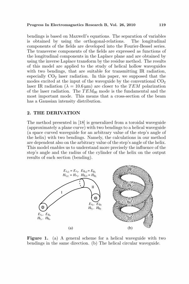
Figure 1. (a) A general scheme for a helical waveguide with twobendings in the same direction. (b) The helical circular waveguide.


Let us assume that the helical waveguide consists of two bendingsin the same direction as shown in Fig. 1(a). The helical circularwaveguide is shown in Fig. 1(b). The main steps for calculations ofthe output fields and the output power transmission in the case ofthe helical waveguide with two bendings in the same direction areintroduced in this derivation, based on the method presented in [18].The coordinates of an arbitrary point on the toroidal system (r, θ, ζ)with a given bending (R) are shown in Fig. 2, where X = R cosφ andY = R sinφ.

Further, we assume that the first bending (Fig. 1(a)) is R1, thelength is ζ1 = (R1φ1)/ cos δp, and the metric coefficient is hζ1 =1 + (r/R1) sin θcos2(δp), where δp is the step’s angle of the helix.Likewise, the radius of the curvature of the second bending is R2,the length is ζ2 = (R2φ2)/ cos δp, and the metric coefficient is hζ2 =1+(r/R2) sin θcos2(δp), as shown in Fig. 1(a). The total length in thiscase is given by ζ = ζ1 + ζ2. The cases for a straight waveguide areobtained by letting R1 →∞ and R2 →∞.

We start by finding the metric coefficients from the helicaltransformation of the coordinates. The helical transformation of thecoordinates is achieved by two rotations and one translation, and is

Z

Y

R

X

θ

φ

ζ

r

Figure 2. A general scheme ofthe toroidal system (r, θ, ζ) andthe curved waveguide.

Z

Z

X

X

YK

ζ

A

Figure 3. Rotations and transla-tion of the orthogonal system (X,ζ, Z) from point A to the orthog-onal system (X,Y, Z) at point K.


given in the form:(

XYZ

)=

(cos(φc) − sin(φc) 0sin(φc) cos(φc) 0

0 0 1

)(1 0 00 cos(δp) − sin(δp)0 sin(δp) cos(δp)

)(r sin θ

0r cos θ

)

+

(R cos(φc)R sin(φc)ζ sin(δp)

), (1)

where ζ is the coordinate along the helix axis, R is the radius of thecylinder, δp is the step’s angle of the helix (see Figs. 3–4(a)), andφc = (ζ cos(δp))/R. Likewise, 0 ≤ r ≤ a + δm, where 2a is theinternal diameter of the cross-section of the helical waveguide, δm is thethickness of the metallic layer, and d is the thickness of the dielectriclayer (see Fig. 4(b)).

Figure 3 shows the rotations and translation of the orthogonalsystem (X, ζ, Z) from point A to the orthogonal system (X, Y, Z) atpoint K . In the first rotation, the ζ and Z axes rotate around the Xaxis of the orthogonal system (X, ζ, Z) at the point A until the Z axisbecomes parallel to the Z axis (Z ‖ Z), and the ζ axis becomes parallelto the X, Y plane (ζ ‖(X,Y )) of the orthogonal system (X,Y, Z) atthe point K. In the second rotation, the X and ζ axes rotate aroundthe Z axis (Z ‖ Z) of the orthogonal system (X, ζ, Z) until X ‖ X andζ ‖ Y . After the two above rotations, we have one translation from theorthogonal system (X, ζ, Z) at the point A to the orthogonal system(X, Y, Z) at the point K.

ZZ

ζA

ζ

'

_

_

ζ

δ

δ

p

p

pδ

2a

cφR

2 πR

substrate

metal layerdielectric layer

air

(a) (b)

Figure 4. (a) Deployment of the helix. (b) A cross-section of thewaveguide (r, θ).


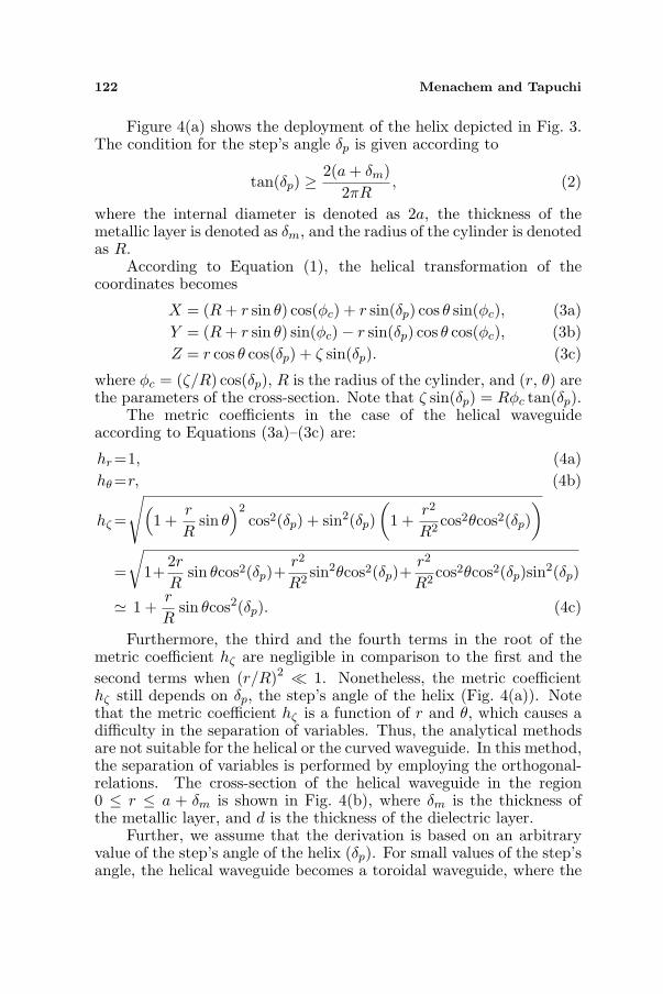
Figure 4(a) shows the deployment of the helix depicted in Fig. 3.The condition for the step’s angle δp is given according to

tan(δp) ≥ 2(a + δm)2πR

, (2)

where the internal diameter is denoted as 2a, the thickness of themetallic layer is denoted as δm, and the radius of the cylinder is denotedas R.

According to Equation (1), the helical transformation of thecoordinates becomes

X = (R + r sin θ) cos(φc) + r sin(δp) cos θ sin(φc), (3a)Y = (R + r sin θ) sin(φc)− r sin(δp) cos θ cos(φc), (3b)Z = r cos θ cos(δp) + ζ sin(δp). (3c)

where φc = (ζ/R) cos(δp), R is the radius of the cylinder, and (r, θ) arethe parameters of the cross-section. Note that ζ sin(δp) = Rφc tan(δp).

The metric coefficients in the case of the helical waveguideaccording to Equations (3a)–(3c) are:

hr =1, (4a)hθ =r, (4b)

hζ =

√(1 +

r

Rsin θ

)2cos2(δp) + sin2(δp)

(1 +

r2

R2cos2θcos2(δp)

)

=

√1+

2r

Rsin θcos2(δp)+

r2

R2sin2θcos2(δp)+

r2

R2cos2θcos2(δp)sin2(δp)

' 1 +r

Rsin θcos2(δp). (4c)

Furthermore, the third and the fourth terms in the root of themetric coefficient hζ are negligible in comparison to the first and thesecond terms when (r/R)2 ¿ 1. Nonetheless, the metric coefficienthζ still depends on δp, the step’s angle of the helix (Fig. 4(a)). Notethat the metric coefficient hζ is a function of r and θ, which causes adifficulty in the separation of variables. Thus, the analytical methodsare not suitable for the helical or the curved waveguide. In this method,the separation of variables is performed by employing the orthogonal-relations. The cross-section of the helical waveguide in the region0 ≤ r ≤ a + δm is shown in Fig. 4(b), where δm is the thickness ofthe metallic layer, and d is the thickness of the dielectric layer.

Further, we assume that the derivation is based on an arbitraryvalue of the step’s angle of the helix (δp). For small values of the step’sangle, the helical waveguide becomes a toroidal waveguide, where the


radius of the curvature of the helix can then be approximated by theradius of the cylinder (R). In this case, the toroidal system (r, θ, ζ)in conjunction with the curved waveguide is shown in Fig. 2, and thetransformation of the coordinates (3(a)–(c)) is given as a special caseof the toroidal transformation of the coordinates, as follows

X = (R + r sin θ) cos(

ζ

R

), (5a)

Y = (R + r sin θ) sin(

ζ

R

), (5b)

Z = r cos θ, (5c)

and the metric coefficients are given by

hr = 1, (6a)hθ = r, (6b)

hζ = 1 +r

Rsin θ. (6c)

The generalization of the method from a toroidal waveguide [18](approximately a plane curve) with two bendings to a helical waveguide(a space curved waveguide for an arbitrary value of the step’s angle ofthe helix) with two bendings is presented in this paper. The derivationis based on Maxwell’s equations for the computation of the EM fieldand the radiation power density at each point during propagation alonga helical waveguide, with a radial dielectric profile. The longitudinalcomponents of the fields are developed into the Fourier-Bessel series.The transverse components of the fields are expressed as a function ofthe longitudinal components in the Laplace transform domain. Finally,the transverse components of the fields are obtained by using theinverse Laplace transform by the residue method, for an arbitrary valueof the step’s angle of the helix (δp).

The wave equations for the electric and magnetic field componentsin the inhomogeneous dielectric medium ε(r) are derived for a lossydielectric media in metallic boundaries of the waveguide. The cross-section of the helical waveguide is shown in Fig. 4(b) for the applicationof the hollow waveguide, in the region 0 ≤ r ≤ a+ δm, where δm is thethickness of the metallic layer, and d is the thickness of the dielectriclayer.

The derivation is given for the lossless case to simplify themathematical expressions. In a linear lossy medium, the solutionis obtained by replacing the permittivity ε by εc = ε − j(σ/ω) inthe solutions for the lossless case, where εc is the complex dielectricconstant, and σ is the conductivity of the medium. The boundaryconditions for a lossy medium are given after the derivation. For most


materials, the permeability µ is equal to that of free space (µ = µ0).The wave equations for the electric and magnetic field components inthe inhomogeneous dielectric medium ε(r) are given by

∇2E + ω2µεE +∇(E · ∇ε

ε

)= 0, (7a)

and

∇2H + ω2µεH +∇ε

ε× (∇×H) = 0, (7b)

respectively. The transverse dielectric profile (ε(r)) is defined asε0(1 + g(r)), where ε0 represents the vacuum dielectric constant, andg(r) is its profile function in the waveguide. The normalized transversederivative of the dielectric profile (gr) is defined as (1/ε(r))(∂ε(r)/∂r).

From the transformation of Equations (3a)–(3c) we can derive theLaplacian of the vector E (i.e., ∇2E), and obtain the wave equationsfor the electric and magnetic fields in the inhomogeneous dielectricmedium. It is necessary to find the values of ∇ · E, ∇(∇ · E),∇× E, and ∇× (∇× E) in order to obtain the value of ∇2E, where∇2E = ∇(∇·E)−∇× (∇×E). All these values are dependent on themetric coefficients ((4a)–(4c)).

The ζ component of ∇2E is given by

(∇2E)ζ = ∇2Eζ +2

Rh2ζ

[sin θ

∂

∂ζEr + cos θ

∂

∂ζEθ

]− 1

R2h2ζ

Eζ , (8)

where

∇2Eζ =∂2

∂r2Eζ +

1r2

∂2

∂θ2Eζ +

1r

∂

∂rEζ

+1hζ

[sin θ

R

∂

∂rEζ +

cos θ

rR

∂

∂θEζ +

1hζ

∂2

∂ζ2Eζ

]. (9)

The longitudinal components of the wave Equations (7a) and (7b) areobtained by deriving the following terms[

∇(E · ∇ε

ε

)]

ζ

=1hζ

∂

∂ζ[Ergr] , (10)

and [∇ε

ε× (∇×H)

]

ζ

= jωε

[∇ε

ε×E

]

ζ

= jωεgrEθ. (11)

The longitudinal components of the wave Equations (7a) and (7b) arethen written in the form

(∇2E)ζ+ k2Eζ +

1hζ

∂

∂ζ(Ergr) = 0, (12)

(∇2H)ζ+ k2Hζ + jωεgrEθ = 0, (13)


where (∇2E)ζ , for instance, is given in Equation (8). The local wavenumber parameter is k = ω

√µε(r) = k0

√1 + g(r), where the free-

space wave number is k0 = ω√

µ0ε0.The transverse Laplacian operator is defined as

∇2⊥ ≡ ∇2 − 1

h2ζ

∂2

∂ζ2. (14)

The Laplace transform

a(s) = L{a(ζ)} =∫ ∞

ζ=0a(ζ)e−sζdζ (15)

is applied on the ζ-dimension, where a(ζ) represents any ζ-dependentvariables, where ζ = (Rφc)/ cos(δp).

The next steps are given in detail in [15, 18], as a part of ourderivation. Let us repeat these main steps, in brief.

The longitudinal components of the fields (Eζ , Hζ) are developedinto Fourier-Bessel series as follows:Eζ(s)=

∑

n′

∑

m′

[An′m′(s)cos(n′θ)+Bn′m′(s)sin(n′θ)

]Jn′

(Pn′m′

r

a

), (16a)

Hζ(s)=∑

n′

∑

m′

[Cn′m′(s)cos(n′θ)+Dn′m′(s)sin(n′θ)

]Jn′

(P ′

n′m′r

a

), (16b)

where Pnm and P ′nm are the mth roots of the equations Jn(x) = 0 and

dJn(x)/dx = 0, respectively.By substituting Equation (8) into Equation (12) and by using

the Laplace transform (15), the longitudinal components of the waveequations (Equations (12) and (13)) are described in the Laplacetransform domain, as coupled wave equations. The transverse fields forthe first section of the helical hollow waveguide with two bendings atζ = ζ1 are obtained directly from the Maxwell equations, and by usingthe Laplace transform (15). The transverse fields for the first sectionof the helical hollow waveguide are dependent only on the longitudinalcomponents of the fields and as function of the step’s angle (δp) of thehelix, as follows:

Er1(s)=1

s2 + k2h2ζ1

{−jωµ0

r

[r

R1cos θcos2(δp)Hζ1 +hζ1

∂

∂θHζ1

]hζ1

+s

[sin θ

R1cos2(δp)Eζ1 +hζ1

∂

∂rEζ1

]+sEr0−jωµ0Hθ0hζ1

}. (17a)

Eθ1(s)=1

s2 + k2h2ζ1

{s

r

[r

R1cos θcos2(δp)Eζ1 + hζ1

∂

∂θEζ1

]

+jωµ0hζ1

[sinθ

R1cos2(δp)Hζ1+hζ1

∂

∂rHζ1

]+sEθ0+jωµ0Hr0hζ1

},(17b)


Hr1(s)=1

s2 + k2h2ζ1

{jωε

r

[r

R1cos θcos2(δp)Eζ1 + hζ1

∂

∂θEζ1

]hζ1

+s

[sin θ

R1cos2(δp)Hζ1 +hζ1

∂

∂rHζ1

]+sHr0 +jωεEθ0hζ1

}, (17c)

Hθ1(s)=1

s2 + k2h2ζ1

{s

r

[r

R1cos θcos2(δp)Hζ1 + hζ1

∂

∂θHζ1

]

−jωεhζ1

[sinθ

R1cos2(δp)Eζ1+hζ1

∂

∂rEζ1

]+sHθ0−jωεEr0hζ1

}, (17d)

where ζ1 is the coordinate along the first section of the helical axis, R1

is the radius of the cylinder of the first section of the helical axis, wherethe metric coefficient is hζ1 = 1 + (r/R1) sin θcos2(δp). The transversefields are substituted into the coupled wave equations. The longitudinalcomponents of the fields are developed into Fourier-Bessel series, inorder to satisfy the metallic boundary conditions of the circular cross-section. The condition is that we have only ideal boundary conditionsfor r = a. Thus, the electric and magnetic fields will be zero inthe metal. Two sets of equations are obtained by substitution thelongitudinal components of the fields into the wave equations. Thefirst set of the equations is multiplied by cos(nθ)Jn(Pnmr/a), and afterthat by sin(nθ)Jn(Pnmr/a), for n 6= 0. Similarly, the second set ofthe equations is multiplied by cos(nθ)Jn(P ′

nmr/a), and after that bysin(nθ)Jn(P ′

nmr/a), for n 6= 0. In order to find an algebraic systemof four equations with four unknowns, it is necessary to integrateover the area (r, θ), where r = [0, a], and θ = [0, 2π], by using theorthogonal-relations of the trigonometric functions. The propagationconstants βnm and β′nm of the TM and TE modes of the hollow

waveguide [19] are given, respectively, by βnm =√

k2o − (Pnm/a)2

and β′nm =√

k2o − (P ′

nm/a)2, where the transverse Laplacian operator

(∇2⊥) is given by −(Pnm/a)2 and −(P ′

nm/a)2 for the TM and TE modesof the hollow waveguide, respectively.

2.1. The Elements of the Boundary Conditions’ Vectors inthe Entrance of the First Section of the Helical Waveguide.

The separation of variables is obtained by using the orthogonal-relations. Thus the algebraic equations (n 6= 0) are given by

α(1)n An + β(1)

n Dn =1π

(BC1)n, (18a)

α(2)n Bn + β(2)

n Cn =1π

(BC2)n, (18b)


β(3)n Bn + α(3)

n Cn =1π

(BC3)n, (18c)

β(4)n An + α(4)

n Dn =1π

(BC4)n. (18d)

Further we assume n′ = n = 1. The elements (α(1)n , β

(1)n , etc), on

the left side of (18a) for n = 1 are given for an arbitrary value of thestep’s angle (δp) for the first section of the helical waveguide by:

α(1)mm′1 = π

(s2 + β2

1m′) [(

s2 + k20

)G

(1)mm′00 + k2

0G(1)mm′01

]

+π1

R41

k20s

2

(14cos4(δp)G

(1)mm′02 +

12cos4(δp)G

(1)mm′03

)

+πk20

{s2G

(1)mm′01 +G

(1)mm′05 +

1R2

1

(G

(1)mm′00 +G

(1)mm′01

)

+3

2R21

β21m′cos4(δp)

(G

(1)mm′02 + G

(1)mm′03

)

+1

4R41

cos4(δp)(G

(1)mm′02 + G

(1)mm′03

)

+1

8R41

cos8(δp)(G

(1)mm′06 +G

(1)mm′07

)}

+πs2

[G

(1)mm′08 +

12R2

1

cos2(δp)G(1)mm′00

+1

4R21

(cos4(δp)β2

1m′G(1)mm′02 + cos2(δp)G

(1)mm′09

)

+1

2R21

P1m′

acos2(δp)

(G

(1)mm′10 +

12cos2(δp)G

(1)mm′11

)]

+πk40cos4(δp)

[3

2R21

(G

(1)mm′03 + G

(1)mm′04

)

+1

8R41

cos8(δp)(G

(1)mm′07 + G

(1)mm′12

)], (19a)

β(1)mm′1 =−jωµ0πs

{G

(1)mm′13 +

(12cos2(δp) +

34cos4(δp)

)1

R21

G(1)mm′14

+(

12

+ cos2(δp))

1R2

1

G(1)mm′15 − 1

2R21

G(1)mm′00

−cos2(δp)1

R21

P ′1m′

aG

(1)mm′16

}, (19b)

where the elements of the matrices (G(1)mm′00 , etc.) are given in


Appendix A. Similarly, the rest of the elements on the left side inEquations (18a)–(18d) are obtained. We establish an algebraic systemof four equations with four unknowns. All the elements of the matricesin the Laplace transform domain are dependent on the step’s angleof the helix (δp), the Bessel functions; the dielectric profile g(r); thetransverse derivative gr(r); and (r, θ).

The elements of the boundary conditions’ vectors on the right sidein Equations (18a)–(18d) are changed at the entrance of every sectionof the helical waveguide with two bendings. These elements are givenin conjunction with the excitation of every section, as follows:

(BC1)1 =∫ 2π

0

∫ a

0(BC1) cos(θ)J1(P1mr/a)rdrdθ, (20a)

(BC2)1 =∫ 2π

0

∫ a

0(BC2) sin(θ)J1(P1mr/a)rdrdθ, (20b)

(BC3)1 =∫ 2π

0

∫ a

0(BC3) cos(θ)J1(P ′

1mr/a)rdrdθ, (20c)

(BC4)1 =∫ 2π

0

∫ a

0(BC4) sin(θ)J1(P ′

1mr/a)rdrdθ. (20d)

In the case of the TEM00 mode in excitation for the first section ofthe helical waveguide with two bendings (Fig. 1(a)), the elements ofthe boundary conditions’ vectors are obtained, where:

BC1 = BC2 = jωµ0H+θ0

sgrh2ζ1 +

2R1

hζ1 sin θ(jωµ0H

+θ0

s + k2E+r0

hζ1

)

+2

R1hζ1 cos θ

(−jωµ0H

+r0

s + k2E+θ0

hζ1

)+ k2h3

ζ1E+r0

gr, (21a)

BC3 = BC4 = −jωεE+θ0

sgrh2ζ1 +

2R1

hζ1 sin θ(k2hζ1H

+r0− jωεsE+

θ0

)

+2

R1hζ1 cos θ

(k2hζ1H

+θ0

+ jωεsE+r0

)+ k2h3

ζ1H+r0

gr. (21b)

The elements of the boundary conditions (e.g., (BC2)1) at ζ = 0+ onthe right side in (18b) are given by

(BC2)1 =[(

s2 + k2h2ζ1

) (sEζ0 + E′

ζ0

)]+ jωµ0Hθ0sgrh

2ζ1

+2

R1hζ1 sin θ

(jωµ0Hθ0s + k2Er0hζ1

)

+2

R1hζ1 cos θ

(−jωµ0Hr0s + k2Eθ0hζ1

)+ k2h3

ζ1Er0gr,

where the metric coefficient is hζ1 = 1 + (r/R1) sin θcos2(δp).


The boundary conditions at ζ1 = 0+ for TEM00 mode inexcitation become to

(BC2)1 = 2π

{∫ a

0Q(r)(k(r) + js)k(r)J1m(P1mr/a)rdr

}δ1n

+4jsπ

R21

cos2(δp){∫ a

0Q(r)k(r)J1m(P1mr/a)r2dr

}δ1n

+9π

2R21

cos4(δp){∫ a

0Q(r)k2(r)J1m(P1mr/a)r3dr

}δ1n

+3jsπ

2R21

cos4(δp){∫ a

0Q(r)k(r)J1m(P1mr/a)r3dr

}δ1n

+8π

R21

cos2(δp){∫ a

0Q(r)k2(r)J1m(P1mr/a)r2dr

}δ1n, (22)

whereQ(r) =

E0

nc(r) + 1gr exp (−(r/wo)

2).

Similarly, the remaining elements of the boundary conditions at ζ = 0+

are obtained. The matrix system of the Equations (18a)–(18d) is solvedto obtain the coefficients (A1, B1, etc).

According to the Gaussian beams [20] the parameter w0 is theminimum spot-size at the plane z = 0, and the electric field atthe plane z = 0 is given by E = E0 exp[−(r/wo)

2]. The modesexcited at ζ = 0 in the waveguide by the conventional CO2 laser IRradiation (λ = 10.6µm) are closer to the TEM polarization of the laserradiation. The TEM00 mode is the fundamental and most importantmode. This means that a cross-section of the beam has a Gaussianintensity distribution. The relation between the electric and magneticfields [20] is given by E/H =

√µ0/ε0 ≡ η0, where η0 is the intrinsic

wave impedance. Suppose that the electric field is parallel to the y-axis. Thus the components of Ey and Hx are written by the fieldsEy = E0 exp[−(r/wo)

2] and Hx = −(E0/η0) exp[−(r/wo)2].

After a Gaussian beam passes through a lens and before it entersto the waveguide, the waist cross-sectional diameter (2w0) can thenbe calculated approximately for a parallel incident beam by meansof w0 = λ/(πθ) ' (fλ)/(πw). This approximation is justified if theparameter w0 is much larger than the wavelength λ. The parameterof the waist cross-sectional diameter (2w0) is taken into account inour method, instead of the focal length of the lens (f). The initialfields at ζ = 0+ are formulated by using the Fresnel coefficients of the


transmitted fields [21] as follows

E+r0

(r, θ, ζ = 0+) = TE(r)(E0e−(r/wo)2 sin θ), (23a)

E+θ0

(r, θ, ζ = 0+) = TE(r)(E0e−(r/wo)2 cos θ), (23b)

H+r0

(r, θ, ζ = 0+) = −TH(r)((E0/η0)e−(r/wo)2 cos θ), (23c)

H+θ0

(r, θ, ζ = 0+) = TH(r)((E0/η0)e−(r/wo)2 sin θ), (23d)

where E+ζ0

(r) = H+ζ0

= 0, TE(r) = 2/[n(r)+1], TH(r) = 2n(r)/[n(r)+1], and n(r) = (εr(r))1/2. The index of refraction is denoted by n(r).The index of refraction is denoted by n(r).

2.2. The Transverse Components of the Fields of the FirstSection of the Helical Waveguide, at ζ = ζ1.

The output transverse components of the fields of the helical waveguideare dependent also on the step’s angle of the helix (δp) and the radiusof the cylinder of the helix for the first section (R1). The outputtransverse components of the fields are finally expressed in a form oftransfer matrix functions for the first bending of the helical waveguideas follows:

Er1(r, θ, ζ1) = E+r0(r)e

−jkhζ1ζ1− jωµ0

R1hζ1cos2 θcos2(δp)

∑

m′Cm′

S1 (ζ1)J1(ψ)

−jωµ0

R1hζ1 sin θ cos θcos2(δp)

∑

m′Dm′

S1(ζ1)J1(ψ)

+jωµ0

rh2

ζ1 sin θ∑

m′Cm′

S1 (ζ1)J1(ψ)

−jωµ0

rh2

ζ1 cos θ∑

m′Dm′

S1(ζ1)J1(ψ)

+1

R1sin θ cos θcos2(δp)

∑

m′Am′

S2(ζ1)J1(ξ)

+1

R1sin2θcos2(δp)

∑

m′Bm′

S2 (ζ1)J1(ξ)

+hζ1 cos θ∑

m′Am′

S2(ζ1)dJ1

dr(ξ)

+hζ1 sin θ∑

m′Bm′

S2 (ζ1)dJ1

dr(ξ), (24)


where hζ1 = 1 + (r/R1) sin θcos2(δp), R is the radius of the cylinder,δp is the the step’s angle, ψ = [P ′

1m′(r/a)] and ξ = [P1m′(r/a)]. Thecoefficients are given in the above equation, for instance

Am′S1(ζ1) = L−1

{A1m′(s)

s2 + k2(r)h2ζ1

}, (25a)

Am′S2(ζ1) = L−1

{sA1m′(s)

s2 + k2(r)h2ζ1

}, (25b)

where

m′ = 1, . . . N, 3 ≤ N ≤ 50. (25c)

Similarly, the other transverse components of the output fields areobtained. The first fifty roots (zeros) of the equations J1(x) = 0 anddJ1(x)/dx = 0 may be found in tables [22, 23].

2.3. The Elements of the Boundary Conditions’ Vectors inthe Entrance of the Second Section of the HelicalWaveguide at ζ = ζ1

The elements of the boundary conditions’ vectors (20a)–(20d) in thecase of the TEM00 mode in excitation for the second section of thehelical waveguide with two bendings are obtained from the algebraicsystem of Equations (18a)–(18d) for n = 1, as follows:

BC1 = BC2 = jωµ0Hθ(ζ = ζ1)sgrh2ζ2

+2

R2sin θhζ2

(jωµ0Hθ(ζ = ζ1)s + k2Er(ζ = ζ1)hζ2

)

+2

R2cos θhζ2

(−jωµ0Hr(ζ = ζ1)s + k2Eθ(ζ = ζ1)hζ2

)

+k2h3ζ2Er(ζ = ζ1)gr, (26a)

BC3 = BC4 = −jωεEθ(ζ = ζ1)sgrh2ζ2

+2

R2sin θhζ2

(k2hζ2Hr(ζ = ζ1)− jωεsEθ(ζ = ζ1)

)

+2

R2cos θhζ2

(k2hζ2Hθ(ζ = ζ1) + jωεsEr(ζ = ζ1)

)

+k2h3ζ2Hr(ζ = ζ1)gr. (26b)

Equations (26a)–(26b) are different from Equations (21a)–(21b)by the initial fields. The initial field, for instance, at the entrance ofthe first section of the helical waveguide at ζ = 0+ is denoted as E+

r0


according to (23a), but the initial field of the second section of thehelical waveguide in the entrance, at ζ = ζ1, is denoted as Er(ζ = ζ1),according to (24). Similarly, the remaining initial fields are obtained.

These expressions (26a), (26b) are dependent on the radius of thecylinder of the helix of the first section (R1) and the second section (R2)of the helical waveguide with two bendings (R1 6= R2). Note that theseexpressions are given also for arbitrary values of the step’s angle (andnot for small values of the step angles). Actually, these expressions((26a), (26b)) for the helical waveguide with two bendings consist ofall the information at the output fields of the first section (the Bessel-equations, the dielectric profile g(r), the transverse derivative gr(r), theparameters of the cross-section (r, θ), and the propagation constantsβnm and β′nm of the TM and TE modes of the hollow waveguide,respectively).

2.4. The Transverse Fields for the Second HelicalWaveguide at ζ = ζ1 + ζ2

The expression [1/(s2 + k2h2ζ1

)](sE+r0− jωµ0H

+θ0

hζ1) in Equation (17a)for the first section of the helical waveguide with two bendings dependson the inital fields E+

r0(23a) and H+

θ0(23d). In the same principle we

have the expression [1/(s2 +k2h2ζ2

)](sEr(ζ = ζ1)− jωµ0Hθ(ζ = ζ1)hζ2)for the second section of the helical waveguide with two bendings, thatdepends on the output fields Er(ζ = ζ1) and Hθ(ζ = ζ1) (e.g., (24)) atζ = ζ1 of the first section of the helical waveguide with two bendings.

The values of the input fields of the second section of the helicalwaveguide with two bendings are functions of the parameters of thefirst section (R1, ζ1, and hζ1) and the second section (R2, ζ2, and hζ2)as shown in Fig. 1(a). The expressions are functions of the cross-section(r, θ), the sum of the modes and the old coefficients of the first sectionof the helical waveguide with two bendings.

The output transverse components of the fields of the helicalwaveguide are dependent also on the step’s angle of the helix (δp)and the radius of the cylinder of the helix for the first section (R1)and for the second section (R2). The output transverse components ofthe fields are finally expressed in a form of transfer matrix functions


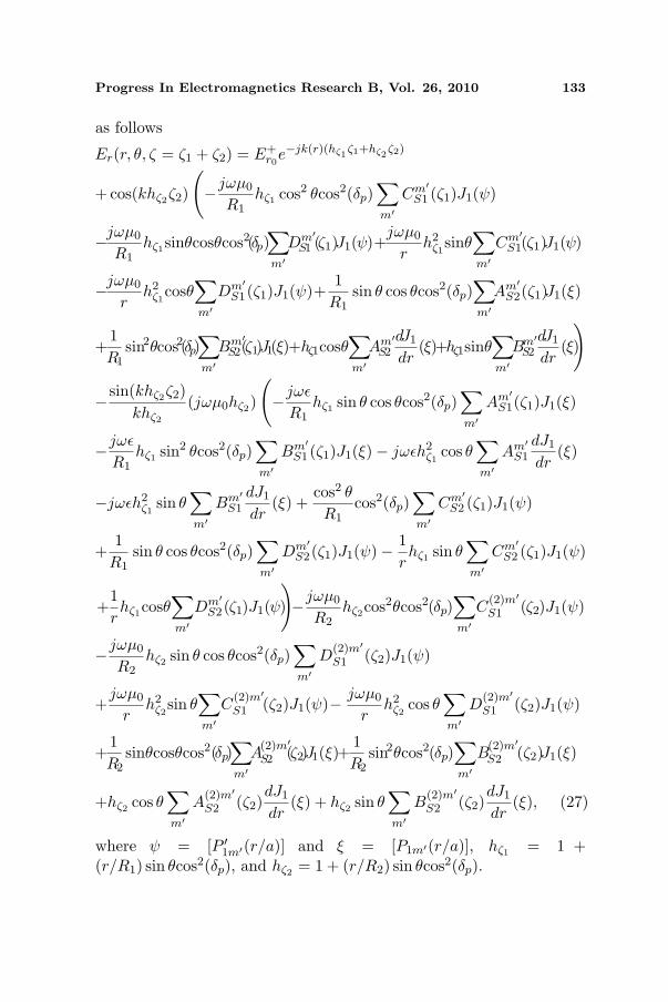
as follows

Er(r, θ, ζ = ζ1 + ζ2) = E+r0

e−jk(r)(hζ1ζ1+hζ2

ζ2)

+cos(khζ2ζ2)

(−jωµ0

R1hζ1 cos2 θcos2(δp)

∑

m′Cm′

S1 (ζ1)J1(ψ)

−jωµ0

R1hζ1sinθcosθcos2(δp)

∑

m′Dm′

S1 (ζ1)J1(ψ)+jωµ0

rh2

ζ1sinθ∑

m′Cm′

S1(ζ1)J1(ψ)

−jωµ0

rh2

ζ1cosθ∑

m′Dm′

S1(ζ1)J1(ψ)+1


∑

m′Am′

S2(ζ1)J1(ξ)

+1R1

sin2θcos2(δp)∑

m′Bm′

S2(ζ1)J1(ξ)+hζ1cosθ∑

m′Am′

S2

dJ1

dr(ξ)+hζ1sinθ

∑

m′Bm′

S2

dJ1

dr(ξ)

)

−sin(khζ2ζ2)khζ2

(jωµ0hζ2)

(−jωε


∑

m′Am′

S1(ζ1)J1(ξ)

−jωε

R1hζ1 sin2 θcos2(δp)

∑

m′Bm′

S1 (ζ1)J1(ξ)− jωεh2ζ1 cos θ

∑

m′Am′

S1

dJ1

dr(ξ)

−jωεh2ζ1 sin θ

∑

m′Bm′

S1

dJ1

dr(ξ) +

cos2 θ

R1cos2(δp)

∑

m′Cm′

S2 (ζ1)J1(ψ)

+1


∑

m′Dm′

S2(ζ1)J1(ψ)− 1rhζ1 sin θ

∑

m′Cm′

S2 (ζ1)J1(ψ)

+1rhζ1cosθ

∑

m′Dm′

S2(ζ1)J1(ψ)

)−jωµ0

R2hζ2cos2θcos2(δp)

∑

m′C

(2)m′S1 (ζ2)J1(ψ)

−jωµ0


∑

m′D

(2)m′S1 (ζ2)J1(ψ)

+jωµ0

rh2

ζ2sin θ∑

m′C

(2)m′S1 (ζ2)J1(ψ)− jωµ0

rh2

ζ2 cos θ∑

m′D

(2)m′S1 (ζ2)J1(ψ)

+1R2

sinθcosθcos2(δp)∑

m′A

(2)m′S2 (ζ2)J1(ξ)+

1R2

sin2θcos2(δp)∑

m′B

(2)m′S2 (ζ2)J1(ξ)

+hζ2 cos θ∑

m′A

(2)m′S2 (ζ2)

dJ1

dr(ξ) + hζ2 sin θ

∑

m′B

(2)m′S2 (ζ2)

dJ1

dr(ξ), (27)

where ψ = [P ′1m′(r/a)] and ξ = [P1m′(r/a)], hζ1 = 1 +

(r/R1) sin θcos2(δp), and hζ2 = 1 + (r/R2) sin θcos2(δp).


The new coefficients are given in the above equation, for instance

A(2)m′S1 (ζ2) = L−1

[A

(2)1m′(s)

s2 + k2(r)h2ζ2

], (28a)

A(2)m′S2 (ζ2) = L−1

[sA

(2)1m′(s)

s2 + k2(r)h2ζ2

], (28b)

wherem′ = 1, . . . N, 3 ≤ N ≤ 50. (28c)

Similarly, the other output transverse components of the fields areobtained, in a form of transfer matrix functions (e.g., Equation (27)).The above general solutions of the output transverse components ofthe fields (e.g., Equation (27)) at ζ = ζ1 + ζ2 are dependent on theinitial fields at ζ = ζ1 along the total length ζ = ζ1 + ζ2, whereζ1 = (R1φ1)/ cos δp and ζ2 = (R2φ2)/ cos δp. Note that the mainexpression of the solution of the output transverse components of thefields (e.g., Equation (24)) is proportional to E+

r0exp[−jk(r)hζ1ζ1].

In the same principle, the main expression for the second sectionof the helical waveguide with two bendings (e.g., Equation (27)) isproportional to E+

r0exp[−jk(r)(hζ1ζ1 + hζ2ζ2)].

These above solutions (e.g., (27)) consist of the sum of theprinciple expression and other expressions. The principle expressionis multiplication of the initial field at ζ = 0+ (23a) with the exponent[exp[−jk(r)(hζ1ζ1 + hζ2ζ2)]]. All the above derivation is introducedin the case of the helical waveguide with two bendings in the samedirection.

The inverse Laplace transform is performed in this study by adirect numerical integration in the Laplace transform domain by theresidue method, as follows

f(ζ) = L−1[f(s)] =1

2πj

∫ σ+j∞

σ−j∞f(s)esζds =

∑n

Res[esζ f(s);Sn]. (29)

By using the inverse Laplace transform (29) we can compute theoutput transverse components in the real plane and the output powerdensity at each point at ζ = (Rφc)/ cos(δp). The integration path in theright side of the Laplace transform domain includes all the singularitiesaccording to Equation (29). All the points Sn are the poles of f(s) andRes[esζ f(s);Sn] represent the residue of the function in a specific pole.According to the residue method, two dominant poles for the helicalwaveguide are given by

s = ±j k(r)hζ = ±j k(r)(1 +

r

Rsin θcos2(δp)

).


Finally, knowing all the transverse components, the ζ componentof the average-power density Poynting vector is given by

Sav =12Re {ErHθ

∗ −EθHr∗} . (30)

where the asterisk indicates the complex conjugate.The total average-power transmitted along the guide in the ζ

direction can be obtained now by the integral of Equation (30) overthe waveguide cross section. Thus, the output power transmission isgiven by

T =12

∫ 2π

0

∫ a

0Re

{ErHθ

∗ −EθHr∗}

rdrdθ. (31)

Lossy Medium CaseIn a linear lossy medium, the solution is obtained by replacing

the permittivity ε by εc = ε − j(σ/ω) in the preceding mathematicalexpressions, where εc is the complex dielectric constant and σ is theconductivity of the medium. The coefficients are obtained directly fromthe algebraic Equations (18a)–(18d) and are expressed as functionsin the Laplace transform domain. To satisfy the metallic boundaryconditions of a circular cross-section we find the new roots P

(new)1m and

P′(new)1m of the equations J1(z) = 0 and dJ1(z)/dz = 0, respectively,

where z is complex. Thus, from the requirement that the coefficientsvanish, the new roots P

(new)1m and P

′(new)1m are calculated by developing

into the Taylor series, in the first order at 1/σ. The new roots in thecase of a lossy medium are complex. The complex Bessel functions arecomputed by using NAG subroutine [24]. The explanation is given indetail in [15].

Several examples computed on a Unix system are presented inthe next section, in order to demonstrate the results of this proposedmethod for the helical waveguide that consists of two bendings. Wesuppose that the transmitted fields of the initial fields (TEM00 modein excitation) are formulated by using the Fresnel coefficients (23a)–(23d).

3. NUMERICAL RESULTS

This section presents several examples that demonstrate features ofthe proposed mode model derived in the previous section. The cross-section of the curved waveguide (Fig. 4(b)) is made of a tube of varioustypes of material, a metallic layer, and a dielectric layer upon it.The next examples represent the case of the hollow waveguide with


a metallic layer (Ag) coated by a thin dielectric layer (AgI). For silverhaving a conductivity of 6.14 ×107 (ohm · m)−1 and the skin depth at10.6µm is 1.207× 10−8 m.

Three test-cases are demonstrated for small values of the step’sangle (δp). In these cases, δp ≥ 2(a + δm)/(2πR), according to thecondition (2). Note that for small values of the step’s angle, the helicalwaveguide becomes approximately a toroidal waveguide (see Fig. 2),where the radius of the curvature of the helix can then be approximatedby the radius of the cylinder (R).

The first test-case is demonstrated for the straight waveguide(R →∞). The results of the output transverse components of the fieldsand the output power density (|Sav|) (e.g., Fig. 5(a)) show the samebehavior of the solutions as shown in the results of [15] for the TEM00

mode in excitation. The result of the output power density (Fig. 5(a))is compared also to the result of published experimental data [25] (seealso in Fig. 5(b)). This comparison shows good agreement (a Gaussianshape) as expected, except for the secondary small propagation mode.The experimental result (Fig. 5(b)) is affected by the additionalparameters (e.g., the roughness of the internal wall of the waveguide)which are not taken theoretically into account. In this example, thelength of the straight waveguide is 1 m, the diameter (2a) of thewaveguide is 2mm, the thickness of the dielectric layer [d(AgI)] is0.75µm, and the minimum spot-size (w0) is 0.3 mm. The refractiveindices of the air, the dielectric layer (AgI) and the metallic layer (Ag)are n(0) = 1, n(AgI) = 2.2, and n(Ag) = 13.5 − j75.3, respectively.The value of the refractive index of the material at a wavelength ofλ = 10.6µm is taken from the table compiled by Miyagi et al. in [6].

The second test-case is demonstrated in Fig. 5(c) for the toroidaldielectric waveguide. Fig. 5(d) shows the experimental result thatwas received in the laboratory of Croitoru at Tel-Aviv University.This experimental result was obtained from the measurements of thetransmitted CO2 laser radiation (λ = 10.6µm) propagation througha hollow tube covered on the bore wall with silver and silver-iodidelayers (Fig. 4(b)), where the initial diameter (ID) is 1 mm (namely,small bore size).

The output modal profile is greatly affected by the bending, andthe theoretical and experimental results (Figs. 5(c)–5(d)) show thatin addition to the main propagation mode, several other secondarymodes and asymmetric output shape appear. The amplitude of theoutput power density (|Sav|) is small as the bending radius (R) issmall, and the shape is far from a Gaussian shape. This result agreeswith the experimental results, but not for all the propagation modes.The experimental result (Fig. 5(d)) is affected by the bending and


-1.0

-0.5

0.0

0.5x [mm] -0.5

0.0

0.5

1.0

y [mm]

0.0

0.2

0.4

0.6

0.8

1.0

-0.6-0.4

-0.2 0

0.2 0.4

x [mm] -0.4

-0.2 0

0.2 0.4

0.6

y [mm]

0 0.1 0.2 0.3 0.4 0.5 0.6

(a) (b)

(c) (d)

|S | [W/m ]av2

|S | [W/m ]av 2

Figure 5. The output power density for R → ∞, where a = 1 mm,w0 = 0.3mm, and the length of the straight waveguide is 1 m: (a)theoretical result; (b) experimental result. The output power densityfor the toroidal dielectric waveguide, where a = 0.5mm, w0 = 0.2mm,R = 0.7m, φ = π/2, and ζ = 1m: (c) theoretical result; (d)experimental result. The other parameters are: d(AgI) = 0.75µm,λ = 10.6µm, n(0) = 1, n(AgI) = 2.2, and n(Ag) = 13.5− j75.

additional parameters (e.g., the roughness of the internal wall of thewaveguide) which are not taken theoretically into account. In thisexample, a = 0.5mm, R = 0.7m, φ = π/2, and ζ = 1 m. The thicknessof the dielectric layer [d(AgI)] is 0.75µm (Fig. 4(b)), and the minimumspot size (w0) is 0.2 mm. The values of the refractive indices of theair, the dielectric layer (AgI) and the metallic layer (Ag) are n(0) = 1,n(AgI) = 2.2, and n(Ag) = 13.5−j75.3, respectively. In both theoreticaland experimental results (Figs. 5(c)–5(d)) the shapes of the outputpower density for the curved waveguide are not symmetric.

The third test-case is demonstrated in Fig. 6 for the toroidalwaveguide. The theoretical mode-model’s result and the experimentalresult [11] are demonstrated in normalized units where the length ofthe curved waveguide (ζ) is 0.55 m, the diameter (2a) of the waveguideis 2.4 mm, and the minimum spot size (w0) is 0.1mm.

This comparison (Fig. 6) between the theoretical mode-model


and the experimental data [11] shows an approximated result. Forall the examples, our theoretical mode-model takes into account onlythe dielectric losses and the bending losses, in conjunction withthe problem of the propagation through a curved waveguide. Theexperimental result [11] takes into account additional parameters (e.g.,the roughness of the internal wall of the waveguide) which are not takentheoretically into account. For small values of the bending (1/R) inthe case of small step’s angle, the output power transmission is largeand decreases with increasing the bending.

0

0.2

0.4

0.6

0.8

1

0 0.5 1 1.5 2

T (

norm

. u

nit

s)

1/R (1/m)

Mode-modelExperimental data

Figure 6. The theoretical mode-model’s result and the experimentalresult [11] where the hollow metallic waveguide (Ag) is covered insidethe walls with a AgI film. The output power transmission as afunction of 1/R for δp = 0, where ζ = 0.55m, where a = 1.2mm,d(AgI) = 0.75µm, w0 = 0.1mm, λ = 10.6µm, n(0) = 1, n(AgI) = 2.2,and n(Ag) = 10.

75

80

85

90

95

100

0.5 1 1.5 2 2.5 3

(%

) T

RA

NS

MIS

SIO

N

R [m]

w 0= 0.06 mm

w 0= 0.15 mm

Figure 7. The output power transmission as a function of the radiusof the cylinder (R) for ζ1 = 1 m in two cases of the spot size: (a)w0 = 0.06mm; (b) w0 = 0.15mm, for δp = 1. The optimum resultis obtained by the first solution of the first section of the helicalwaveguide.


75

80

85

90

95

100

0.6 0.8 1 1.2 1.4 1.6 1.8 2

(%

) T

RA

NS

MIS

SIO

N

1/R (1/m)

δp = 0.0

δp = 0.2

δp = 0.4

δp = 0.6

δp = 0.8

δp = 1 75

80

85

90

95

100

0.5 1 1.5 2 2.5 3

(%

) T

RA

NS

MIS

SIO

N

R [m]

δp = 0.0

δp = 0.2

δp = 0.4

δp = 0.6

δp = 0.8

δp = 1

(a) (b)

Figure 8. (a) The output power transmission of the helical waveguideas a function of 1/R, where R is the radius of the cylinder. (b) Theoutput power transmission of the helical waveguide as a function ofR. Six results are demonstrated for six values of δp (δp = 0, 0.2, 0.4,0.6, 0.8, 1), where ζ = 1 m, a = 1mm, w0 = 0.06mm, nd = 2.2, andn(Ag) = 13.5− j75.3.

The contribution of this paper is demonstrated in Figs. 7, 8(a),8(b), 9(a)–9(e) and in Figs. 10(a)–10(e), in order to understand theinfluence of the step’s angle (δp) and the radius of the cylinder (R) onthe output power transmission, as defined in Equation (31), and theoutput fields. Fig. 7 represents the effect of the radius of the cylinderon the output power transmission for the first section of the helicalwaveguide (Fig. 1(a)), for δp = 1, where δp is the step’s angle of thehelix. The output power transmission as a function of the radius of thecylinder (R) of the helix is shown in Fig. 7 where the length of the firstsection of the helical waveguide (ζ1) is 1 m, and where the values ofthe spot-size (w0) are 0.06mm and 0.15 mm. The diameter (2a) of thewaveguide is 2 mm, and the value of the refractive index of the materialat a wavelength of λ = 10.6µm. The output power transmission (T )is at least equal to 75% (75% ≤ T ≤ 100%). The optimum result isobtained where the spot-size (w0) is 0.06mm.

Figure 8(a) demonstrates the influence of the step’s angle andthe bending (1/R) on the output power transmission. Fig. 8(b)demonstrates the influence of the step’s angle and the radius of thecylinder (R) on the output power transmission. Figs. 8(a) and 8(b)are demonstrated for six values of δp (δp = 0, 0.2, 0.4, 0.6, 0.8, 1),where the length of the first section of the helical waveguide (ζ1) is 1 m,and where the values of the spot-size (w0) is 0.06 mm. The diameter(2a) of the waveguide is 2 mm, and the value of the refractive indexof the material at a wavelength of λ = 10.6µm. The output powertransmission (T ) is at least equal to 75% (75% ≤ T ≤ 100%).


-1

-0.5 0

0.5x [mm]

-1

-0.5

0

0.5

1

y [mm]

0 100 200 300 400 500 600

-1

-0.5 0

0.5x [mm]

-1

-0.5

0

0.5

1

y [mm]

0 100 200 300 400 500 600 700

-1

-0.5 0

0.5x [mm]

-1

-0.5

0

0.5

1

y [mm]

0 0.2 0.4 0.6 0.8

1 1.2 1.4 1.6

-1

-0.5 0

0.5x [mm]

-1

-0.5

0

0.5

1

y [mm]

0 0.2 0.4 0.6 0.8

1 1.2 1.4 1.6 1.8

-1

-0.5 0

0.5x [mm]

-1

-0.5

0

0.5

1

y [mm]

0 0.1 0.2 0.3 0.4 0.5 0.6 0.7 0.8 0.9

(a) (b)

(c) (d)

(e)

|S | [W/m ]av2

|E | [V/m]r |E | [V/m]θ

|H | [A/m]r |H | [A/m]θ

Figure 9. The solution of the output transverse components (a)–(d),and the output power density (e) in the case of the helical waveguidewith two bendings, where δp = 0.5, R1 = 0.5m and R2 = 0.4 m,φ1 = π, φ2 = π/2, a = 1mm, d(AgI) = 0.75 µm, λ = 10.6µm,w0 = 0.06mm, n(0) = 1, n(AgI) = 2.2, and n(Ag) = 13.5− j75.3.

For an arbitrary value of R, the output power transmission islarge for large values of δp and decreases with decreasing the value ofδp. On the other hand, for an arbitrary value of δp, the output powertransmission is large for large values of R and decreases with decreasingthe value of R. Note that for small values of the step’s angle, the radiusof the curvature of the helix can be approximated by the radius of thecylinder (R). In this case, the output power transmission is large forsmall values of the bending (1/R), and decreases with increasing thebending. Thus, this model can be a useful tool to find the parameters(δp and R) which will give us the improved results (output powertransmission) of a helical hollow waveguide in the cases of space curvedwaveguides.


-1

-0.5 0

0.5x [mm]

-1

-0.5

0

0.5

1

y [mm]

0 100 200 300 400 500 600 700

-1

-0.5 0

0.5x [mm]

-1

-0.5

0

0.5

1

y [mm]

0 100 200 300 400 500 600 700

-1

-0.5 0

0.5x [mm]

-1

-0.5

0

0.5

1

y [mm]

0 0.2 0.4 0.6 0.8

1 1.2 1.4 1.6 1.8

-1

-0.5 0

0.5x [mm]

-1

-0.5

0

0.5

1

y [mm]

0 0.2 0.4 0.6 0.8

1 1.2 1.4 1.6 1.8

-1

-0.5 0

0.5x [mm]

-1

-0.5

0

0.5

1

y [mm]

0 0.1 0.2 0.3 0.4 0.5 0.6 0.7 0.8 0.9

1

(a) (b)

(c) (d)

(e)

|S | [W/m ]av 2

|E | [V/m]r |E | [V/m]θ

|H | [A/m]r |H | [A/m]θ

Figure 10. The solution of the output transverse components (a)–(d),and the output power density (e) in the case of the helical waveguidewith two bendings, where δp = 1, R1 = 0.5m and R2 = 0.4 m,φ1 = π, φ2 = π/2, a = 1 mm, d(AgI) = 0.75 µm, λ = 10.6µm,w0 = 0.06mm, n(0) = 1, n(AgI) = 2.2, and n(Ag) = 13.5− j75.3.

Figures 9(a)–9(e) show the results of the output transversecomponents and the output power density of the field where δp = 0.5,R1 = 0.5 m and R2 = 0.4m, φ1 = π, φ2 = π/2, a = 1 mm,d(AgI) = 0.75µm, λ = 10.6µm, w0 = 0.06 mm, n(0) = 1, n(AgI) = 2.2,and n(Ag) = 13.5 − j75.3. The output transverse components of thefield show that in addition to the main propagation mode, several othersecondary modes appear.

By increasing only the parameter of the step’s angle of the helicalwaveguide with two bendings (R1 = 0.5m, R2 = 0.4m) from δp = 0.5to δp = 1, the results of the output transverse components and theoutput power density of the field are changed, as shown in Figs. 10(a)–10(e). The amplitude of the output power density in Fig. 9(e) is smaller


as regard to the amplitude of the output power density in Fig. 10(e).The amplitude is small as the step’s angle of the helical waveguide issmall.

The output results are greatly affected by the step’s angle, by theradius of the cylinder of the helix, and by the spot size (w0). This modemodel can be a useful tool in order to determine the optimal conditionsfor practical applications (output fields, output power density andoutput power transmission as function of the step’s angle and theradius of the cylinder of the helix). This mode model can be a usefultool to improve the output results in all the cases of the helical hollowwaveguides with two bendings for industrial and medical regimes.

4. CONCLUSIONS

The main objective was to generalize the method [18] to provide anumerical tool for the calculation of the output transverse fields and theoutput power density in the case of the helical waveguide that consistsof two bendings in the same direction, as shown in Fig. 1(a). The mainsteps of the method for the helical waveguide with two bendings aregiven in the derivation, in detail, for an arbitrary value of the step’sangle of the helix.

Three test-cases were demonstrated for small values of the step’sangle (δp). In these cases, δp ≥ 2(a + δm)/(2πR), according to thecondition (2). Note that for small values of the step’s angle, the helicalwaveguide becomes approximately a toroidal waveguide (see Fig. 2),where the radius of the curvature of the helix can then be approximatedby the radius of the cylinder (R).

The first test-case was demonstrated for the straight waveguide(R →∞). The results of the output transverse components of the fieldsand the output power density (|Sav|) (e.g., Fig. 5(a)) show the samebehavior of the solutions as shown in the results of [15] for the TEM00

mode in excitation. The result of the output power density (Fig. 5(a))was compared also to the result of published experimental data [25] (seealso in Fig. 5(b)). This comparison shows good agreement (a Gaussianshape) as expected, except for the secondary small propagation mode.The experimental result (Fig. 5(b)) is affected by the additionalparameters (e.g., the roughness of the internal wall of the waveguide)which are not taken theoretically into account.

The second test-case was demonstrated in Fig. 5(c) for the toroidalwaveguide, and Fig. 5(d) shows the experimental result. The outputmodal profile is greatly affected by the bending, and the theoreticaland experimental results (Figs. 5(c)–5(d)) show that in additionto the main propagation mode, several other secondary modes and


asymmetric output shape appear. The amplitude of the output powerdensity (|Sav|) is small as the bending radius (R) is small, and the shapeis far from a Gaussian shape. This result agrees with the experimentalresults, but not for all the propagation modes. The experimental result(Fig. 5(d)) is affected by the bending and additional parameters (e.g.,the roughness of the internal wall of the waveguide) which are nottaken theoretically into account. In both theoretical and experimentalresults (Figs. 5(c)–5(d)) the shapes of the output power density forthe curved waveguide are not symmetric.

The third test-case was demonstrated in Fig. 6 for the toroidaldielectric waveguide. This comparison (Fig. 6) between the theoreticalmode-model and the experimental data [11] shows an approximatedresult. For all the examples, our theoretical mode-model takes intoaccount only the dielectric losses and the bending losses, in conjunctionwith the problem of the propagation through a curved waveguide. Theexperimental result [11] takes into account additional parameters (e.g.,the roughness of the internal wall of the waveguide) which are not takentheoretically into account. For small values of the bending (1/R) inthe case of small step’s angle, the output power transmission is largeand decreases with increasing the bending.

The contribution of this paper is demonstrated in Figs. 7, 8(a),8(b), 9(a)–9(e) and in Figs. 10(a)–10(e), in order to understand theinfluence of the step’s angle (δp) and the radius of the cylinder (R)on the output power transmission. Fig. 7 represents the effect of theradius of the cylinder on the output power transmission for the firstsection of the helical waveguide (Fig. 1(a)), for δp = 1, where δp is thestep’s angle of the helix. The output power transmission as a functionof the radius of the cylinder (R) of the helix is shown in Fig. 7 wherethe length of the first section of the helical waveguide (ζ1) is 1 m, andwhere the values of the spot-size (w0) are 0.06 mm and 0.15 mm.

Figure 8(a) demonstrates the influence of the step’s angle andthe bending (1/R) on the output power transmission. Fig. 8(b)demonstrates the influence of the step’s angle and the radius of thecylinder (R) on the output power transmission. Figs. 8(a) and 8(b)are demonstrated for six values of δp (δp = 0, 0.2, 0.4, 0.6, 0.8, 1),where the length of the first section of the helical waveguide (ζ1)is 1 m, and where the values of the spot-size (w0) is 0.06mm. InFigs. 7, 8(a), and 8(b), the diameter (2a) of the waveguide is 2 mm,and the value of the refractive index of the material at a wavelengthof λ = 10.6µm. The output power transmission (T ) is at least equalto 75% (75% ≤ T ≤ 100%).

For an arbitrary value of R, the output power transmission islarge for large values of δp and decreases with decreasing the value


of δp. On the other hand, for an arbitrary value of δp, the outputpower transmission is large for large values of R and decreases withdecreasing the value of R. Note that for small values of the step’sangle, the radius of curvature of the helix can be approximated by theradius of the cylinder (R). In this case, the output power transmissionis large for small values of the bending (1/R), and decreases withincreasing the bending. Thus, this model can be a useful tool to findthe parameters (δp and R) which will give us the improved results(output power transmission) of a helical hollow waveguide in the casesof space curved waveguides.

The output transverse components of the field (Figs. 9(a)–9(d))show that in addition to the main propagation mode, several othersecondary modes appear. The output power density of the field isshown in Fig. 9(e). The output results are greatly affected by thestep’s angle, by the radius of the cylinder of the helix, and by the spotsize (w0).

By increasing only the parameter of the step’s angle of the helicalwaveguide with two bendings (R1 = 0.5m, R2 = 0.4m) from δp = 0.5to δp = 1, the output transverse components and the output powerdensity of the field are changed. The amplitude is small as the step’sangle of the helical waveguide is small.

This mode model can be a useful tool in order to determine theoptimal conditions for practical applications (output fields, outputpower density and output power transmission as function of the step’sangle and the radius of the cylinder of the helix). This mode modelcan be a useful tool to improve the output results in all the cases of thehelical hollow waveguides with two bendings for industrial and medicalregimes.

APPENDIX A.

The elements of the matrices (G(1)mm′00 , etc.) are given by:

G(1)mm′00 =

∫ a

0J1

(P1m′

r

a

)J1

(P1m

r

a

)rdrδ1n,

G(1)mm′01 =

∫ a

0g(r)J1

(P1m′

r

a

)J1

(P1m

r

a

)rdrδ1n,

G(1)mm′02 =

∫ a

0J1

(P1m′

r

a

)J1

(P1m

r

a

)r3drδ1n,

G(1)mm′03 =

∫ a

0g(r)J1

(P1m′

r

a

)J1

(P1m

r

a

)r3drδ1n,


G(1)mm′04 =

∫ a

0g2(r)J1

(P1m′

r

a

)J1

(P1m

r

a

)r3drδ1n,

G(1)mm′05 =

∫ a

0k2g(r)J1

(P1m′

r

a

)J1

(P1m

r

a

)rdrδ1n,

G(1)mm′06 =

∫ a

0J1

(P1m′

r

a

)J1

(P1m

r

a

)r5drδ1n,

G(1)mm′07 =

∫ a

0g(r)J1

(P1m′

r

a

)J1

(P1m

r

a

)r5drδ1n,

G(1)mm′08 =

∫ a

0gr

(P1m′

a

)J1′(P1m′

r

a

)J1

(P1m

r

a

)rdr,

G(1)mm′09 =

∫ a

0grJ1

(P1m′

r

a

)J1

(P1m

r

a

)r2drδ1n,

G(1)mm′10 =

∫ a

0J1′(

P1m′r

a

)J1

(P1m

r

a

)r2drδ1n,

G(1)mm′11 =

∫ a

0grJ1

′(

P1m′r

a

)J1

(P1m

r

a

)r3drδ1n,

G(1)mm′12 =

∫ a

0g2(r)J1

(P1m′

r

a

)J1

(P1m

r

a

)r5drδ1n,

G(1)mm′13 =

∫ a

0grJ1

′(

p′1m′r

a

)J1

(P1m

r

a

)drδ1n,

G(1)mm′14 =

∫ a

0grJ1

(p′1m′r

a

)J1

(P1m

r

a

)r2drδ1n,

G(1)mm′15 =

∫ a

0J1

(P ′

1m′r

a

)J1

(P1m

r

a

)rdrδ1n,

G(1)mm′16 =

∫ a

0J1′(

P ′1m′r

a

)J1

(P1m

r

a

)r2drδ1n.

Similarly, the remaining elements are obtained. The coefficientsare obtained directly from the algebraic system of equations (18a)–(18d) and are expressed as functions in s-plane. Similarly, the othercoefficients are obtained.

REFERENCES

1. Harrington, J. A. and Y. Matsuura, “Review of hollow waveguidetechnology,” SPIE, Vol. 2396, 1995

2. Harrington, J. A., D. M. Harris, and A. Katzir (eds.), BiomedicalOptoelectronic Instrumentation, 4–14, 1995.


3. Harrington, J. A., “A review of IR transmitting, hollowwaveguides,” Fiber and Integrated Optics, Vol. 19, 211–228, 2000.

4. Marcatili, E. A. J. and R. A. Schmeltzer, “Hollow metallic anddielectric waveguides for long distance optical transmission andlasers,” Bell Syst. Tech. J., Vol. 43, 1783–1809, 1964.

5. Marhic, M. E., “Mode-coupling analysis of bending losses in IRmetallic waveguides,” Appl. Opt., Vol. 20, 3436–3441, 1981.

6. Miyagi, M., K. Harada, and S. Kawakami, “Wave propagationand attenuation in the general class of circular hollow waveguideswith uniform curvature,” IEEE Trans. Microwave Theory Tech.,Vol. 32, 513–521, 1984.

7. Croitoru, N., E. Goldenberg, D. Mendlovic, S. Ruschin, andN. Shamir, “Infrared chalcogenide tube waveguides,” SPIE,Vol. 618, 140–145, 1986.

8. Melloni, A., F. Carniel, R. Costa, and M. Martinelli,“Determination of bend mode characteristics in dielectricwaveguides,” J. Lightwave Technol., Vol. 19, 571–577, 2001.

9. Bienstman, P., M. Roelens, M. Vanwolleghem, and R. Baets,“Calculation of bending losses in dielectric waveguides usingeigenmode expansion and perfectly matched layers,” IEEEPhoton. Technol. Lett., Vol. 14, 164–166, 2002.

10. Mendlovic, D., E. Goldenberg, S. Ruschin, J. Dror, andN. Croitoru, “Ray model for transmission of metallic-dielectrichollow bent cylindrical waveguides,” Appl. Opt., Vol. 28, 708–712,1989.

11. Morhaim, O., D. Mendlovic, I. Gannot, J. Dror, and N. Croitoru,“Ray model for transmission of infrared radiation throughmultibent cylindrical waveguides,” Opt. Eng., Vol. 30, 1886–1891,1991.

12. Kark, K. W., “Perturbation analysis of electromagnetic eigen-modes in toroidal waveguides,” IEEE Trans. Microwave TheoryTech., Vol. 39, 631–637, 1991.

13. Lewin, L., D. C. Chang, and E. F. Kuester, ElectromagneticWaves and Curved Structures, Chap. 6, 58–68, Peter PeregrinusLtd., London, 1977.

14. Menachem, Z., “Wave propagation in a curved waveguide with ar-bitrary dielectric transverse profiles,” Journal of ElectromagneticWaves and Applications, Vol. 17, No. 10, 1423–1424, 2003, andProgress In Electromagnetics Research, Vol. 42, 173–192, 2003.

15. Menachem, Z., N. Croitoru, and J. Aboudi, “Improved modemodel for infrared wave propagation in a toroidal dielectric


waveguide and applications,” Opt. Eng., Vol. 41, 2169–2180, 2002.16. Menachem, Z. and M. Mond, “Infrared wave propagation

in a helical waveguide with inhomogeneous cross section andapplications,” Progress In Electromagnetics Research, Vol. 61,159–192, 2006.

17. Menachem, Z. and M. Haridim, “Propagation in a helicalwaveguide with inhomogeneous dielectric profiles in rectangularcross section,” Progress In Electromagnetics Research B, Vol. 16,155–188, 2009.

18. Menachem, Z., “Flexible hollow waveguide with two bendingsfor small values of step angles, and applications,” Progress InElectromagnetics Research B, Vol. 21, 347–383, 2010.

19. Collin, R. E., Foundation for Microwave Engineering, McGraw-Hill, New York, 1996.

20. Yariv, A., Optical Electronics, 3rd edition, Holt-Saunders Int.Editions, 1985.

21. Baden Fuller, A. J., Microwaves, Chap. 5, 118–120, PergamonPress, A. Wheaton and Co. Ltd, Oxford, 1969.

22. Olver, F. W. J., Royal Society Mathematical Tables, Zeros andAssociated Values, 2–30, University Press Cambridge, 1960.

23. Jahnke, E. and F. Emde, Tables of Functions with Formulae andCurves, Chap. 8, 166, Dover Publications, New York, 1945.

24. The Numerical Algorithms Group (NAG) Ltd., Wilkinson House,Oxford, U.K..

25. Croitoru, N., A. Inberg, M. Oksman, and M. Ben-David, “Hollowsilica, metal and plastic waveguides for hard tissue medicalapplications,” SPIE, Vol. 2977, 30–35, 1997.

helical waveguide with two bendings, and applications …

Documents