heightening walking above its pedestrian status: walking ... · heightening walking above its...
TRANSCRIPT

University of CaliforniaCenter for EconomicCompetitiveness in
Transportation
2016
Heightening Walking above itsPedestrian Status: Walking and Travel Behavior in California
Final Report UCCONNECT 2016 - TO 015 - 65A0529
Evelyn Blumenberg; Professor; University of California, Los AngelesKate Bridges; Masterʼs Candidate; University of California, Los AngelesMadeline Brozen, Associate Director, University of California, Los AngelesCarole Turley Voulgaris; Ph.D Candidate; University of California, Los Angeles
Sponsored by
Heightening Walking above its
Pedestrian Status:
Walking and Travel Behavior in
California
Evelyn Blumenberg, Kate Bridges, Madeline Brozen, and Carole Turley
Voulgaris
Institute of Transportation Studies, Luskin School of Public Affairs,
University of California, Los Angeles
June 30, 2016
TO 015 65A0529
i
DISCLAIMER STATEMENT
This document is disseminated in the interest of information exchange. The contents of this
report reflect the views of the authors who are responsible for the facts and accuracy of the
data presented herein. The contents do not necessarily reflect the official views or policies of
the State of California. This publication does not constitute a standard, specification or
regulation. This report does not constitute an endorsement by the Department of any product
described herein.
For individuals with sensory disabilities, this document is available in alternate formats. For
information, call (916) 654-8899, TTY 711, or write to California Department of
Transportation, Division of Research, Innovation and System Information, MS-83, P.O. Box
942873, Sacramento, CA 94273-0001.
ii
Table of Contents
LIST OF TABLES .............................................................................................................................................. V
LIST OF FIGURES ........................................................................................................................................... VI
LIST OF MAPS ............................................................................................................................................... VIII
EXECUTIVE SUMMARY ...............................................................................................................................IX
I. ONE STEP AT A TIME: INTRODUCTION .......................................................................................... 1
References .......................................................................................................................................................... 9
II. ARE THESE STREETS MADE FOR WALKING? WALKING AND THE BUILT
ENVIRONMENT IN CALIFORNIA .......................................................................................................... 12
Introduction .................................................................................................................................................... 12
Literature review: Walking and the built environment ......................................................................... 13
Density ......................................................................................................................................................... 13
Proximity to destinations ........................................................................................................................ 14
Diversity of land use ................................................................................................................................. 14
Street connectivity .................................................................................................................................... 15
Walkability composite measures ........................................................................................................... 16
Transportation versus leisure walking .................................................................................................. 17
Data and descriptive analysis ...................................................................................................................... 17
Modeling methodology ................................................................................................................................. 24
Model results .................................................................................................................................................. 27
Discussion ........................................................................................................................................................ 31
Conclusion ...................................................................................................................................................... 32
References ....................................................................................................................................................... 33

iii
III. THE INCREASE IN WALKING: WHAT ROLE FOR THE BUILT ENVIRONMENT? ........... 38
Introduction .................................................................................................................................................... 38
Change in walking .......................................................................................................................................... 39
Data .................................................................................................................................................................. 41
Methodology ................................................................................................................................................... 44
Descriptive analysis ....................................................................................................................................... 46
Model results .................................................................................................................................................. 52
Discussion ........................................................................................................................................................ 60
Conclusion ...................................................................................................................................................... 63
References ....................................................................................................................................................... 64
IV. CHANGE, CHANGE, CHANGE: THE RELATIONSHIP BETWEEN CHANGES IN
NEIGHBORHOOD CHARACTERISTICS AND CHANGES IN WALKING ................................. 67
Introduction .................................................................................................................................................... 67
Determinants of changes in walking mode share ................................................................................... 67
Data and methodology ................................................................................................................................. 70
Results .............................................................................................................................................................. 77
Discussion of results ..................................................................................................................................... 78
Conclusion ...................................................................................................................................................... 79
References ....................................................................................................................................................... 81
V. STRUTTING INTO PRACTICE: WALKING AND TRAVEL DEMAND MODELING .......... 85
Introduction .................................................................................................................................................... 85
Travel demand models: The basics ............................................................................................................ 88

iv
Methodology ................................................................................................................................................... 90
Improving walking in regional travel demand forecasts in major California regions ...................... 91
Quality of mode choice data .................................................................................................................. 91
Quality of the modeled relationship between capacity and demand ............................................ 92
Quality of infrastructure data ................................................................................................................. 94
Geographic coarseness of large-scale models .................................................................................... 95
Quality of route choice data ................................................................................................................... 96
Discussion and conclusion ........................................................................................................................... 97
References ....................................................................................................................................................... 99
APPENDIX A. STUDIES ON CHANGES IN WALKING IN THE UNITED STATES ............... 102
APPENDIX B: ALTERNATIVE MODEL RESULTS .............................................................................. 104
APPENDIX C. WALK SCORE®, NEIGHBORHOOD TYPE, AND SPRAWL ........................... 105
Walk Score® ................................................................................................................................................ 105
Overall study area ................................................................................................................................... 105
MSA ............................................................................................................................................................ 107
Neighborhood typology ............................................................................................................................. 111
Nodal degree ................................................................................................................................................ 119
APPENDIX D. WALK SCORE® BY COUNTY ................................................................................. 120
APPENDIX E. WALK SCORE® BY METROPOLITAN REGION .................................................. 124
APPENDIX F. INTERVIEW PROTOCOL ............................................................................................ 128

v
List of tables
Table 1. Variables included in logistic regression model ...................................................................... 26
Table 2. MSA effects and logistic regression model fit .......................................................................... 27
Table 3. Relationships between built environment characteristics and the odds of walking ....... 28
Table 4. Relationships between control variables and the odds of walking ..................................... 30
Table 5. Differences in sample sizes between survey years ................................................................. 42
Table 6. Correlations between trip origin and destination characteristics ...................................... 45
Table 7. Akaike Information Criterion (AIC) scores comparing model fit by neighborhood
variables .................................................................................................................................................. 46
Table 8. Observed changes between survey sample years .................................................................. 51
Table 9. Logistic regression predicting the odds that a trip will be a walk trip............................... 53
Table 10. Changes that would be expected to increase walking and compared to actual changes
.................................................................................................................................................................. 61
Table 11. Differences in sample sizes between survey years............................................................... 70
Table 12. Number of California census tracts meeting selected thresholds for survey-day trips
.................................................................................................................................................................. 73
Table 13. Change in walking mode shares within sample tracts ......................................................... 73
Table 14. Characteristics of tracts in study sample and within California ........................................ 74
Table 15. Correlations between walking mode share and among its potential predictors .......... 76
Table 16. Results of Tobit regression model predicting change in walking mode share ............... 77
Table 17. Metropolitan Planning Organizations selected for interviews ........................................... 90
Table 18. Number of households between CA travel survey years .................................................. 92
Table 19. Percent land area and population by Walk Score®--Overall study area ....................... 106
Table 20. Walk Score® —Study area and MSA .................................................................................... 107
Table 21. Walk Score® Composition by MSA, Percent Land Area and Percent Population ..... 108

vi
Table 22. Variables included in neighborhood classification analysis ............................................... 112
Table 23. Average built environment characteristics by neighborhood type ................................ 114
Table 24. Walk Score® distribution: Los Angeles county (Los Angeles MSA) .............................. 121
Table 25. Walk Score® distribution: Orange county (Los Angeles MSA) ...................................... 121
Table 26. Walk Score® distribution: San Diego county (San Diego MSA) ..................................... 121
Table 27. Walk Score® distribution: San Francisco county (Bay Area MSA) ................................. 122
Table 28. Walk Score® distribution: Alameda county (Bay Area MSA) .......................................... 122
Table 29. Walk Score® distribution: Contra Costa county (Bay Area MSA) ................................ 122
Table 30. Walk Score® distribution: Marin county (Bay Area MSA) ............................................... 122
Table 31. Walk Score® distribution: San Mateo county (Bay Area MSA) ...................................... 123
Table 32. Walk Score® distribution: Sacramento county (Sacramento MSA) ............................... 123
Table 33. Walk Score® distribution: El Dorado county (Sacramento MSA) .................................. 123
Table 34. Walk Score® distribution: Placer county (Sacramento MSA) ......................................... 123
Table 35. Walk Score® distribution: Yolo county (Sacramento MSA) ............................................ 123
List of figures
Figure 1. Increase in walking mode share by metropolitan area – 2001 to 2012 ............................. 4
Figure 2. Walking mode share by MSA ..................................................................................................... 18
Figure 3. Distribution of walk trips and non-walk trips by trip purpose .......................................... 19
Figure 4. Differences in individual-level characteristics between walkers and non-walkers......... 20
Figure 5. Youngest household member by walking and non-walking households. ......................... 21
Figure 6. Distribution of walk trips and non-walk trips by neighborhood type .............................. 22
Figure 7. Walking mode share by neighborhood type .......................................................................... 22
Figure 8. Average Walk Score® for the origin block groups of walk trips and non-walk trips ... 23

vii
Figure 9. Relationship between a block group's Walk Score®, street network connectivity and
walking mode share .............................................................................................................................. 23
Figure 10. Box plots of variation in Walk Score® and street network connectivity by
neighborhood type ............................................................................................................................... 24
Figure 11. Effects of MSA on the odds of walking .................................................................................. 28
Figure 12. Conceptual Model ..................................................................................................................... 44
Figure 13. Changes in mode shares within the study area, 2001-2012 ............................................. 46
Figure 14. Increases in walking mode share by metropolitan area, 2001-2012 ............................... 47
Figure 15. Changes in trip distance by mode and year, 2001-2012.................................................... 48
Figure 16. Distribution of walk trips among trip purposes, 2001-2012 ............................................ 49
Figure 17. Changes driver's license status among walkers and non-walkers, 2001-2012 ............. 49
Figure 18. Changes in employment status among walkers and non-walkers, 2001-2012 ............. 50
Figure 19. Changes in vehicle availability among walkers and non-walkers, 2001-2012 ................ 50
Figure 20. Effect of age on the probability of walking............................................................................ 54
Figure 21. Effects of licensure, employment, disability, and vehicle availability on the odds of
walking ..................................................................................................................................................... 55
Figure 22. Effects of block-group characteristics on the odds of walking ......................................... 56
Figure 23. Changes in the relationship between trip distance and the odds of walking, 2001-
2012 ......................................................................................................................................................... 56
Figure 24. Effects of trip purpose on the odds of walking .................................................................... 58
Figure 25. Effect of household size on the odds of walking ................................................................. 58
Figure 26. Effect of the presence of children on the odds of walking ............................................... 59
Figure 27. Effects of metropolitan area on the odds of walking ......................................................... 60
Figure 28. Increase in walking attributable to changes in trip, individual, household, and
neighborhood characteristics ............................................................................................................. 62
viii
Figure 29. Distributions of walking mode shares in sample tracts, 2001-2012 ............................... 74
Figure 30. Increase in walking attributable to changes in trip, individual, household, and
neighborhood characteristics ............................................................................................................. 86
Figure 31. Composition of land area and population by Walk Score® categories ........................ 106
Figure 32. Distribution of land use and population by Walk Score® categories and by study
region .................................................................................................................................................... 109
Figure 33. Walkable land area by county ............................................................................................... 110
Figure 34. Population in walkable areas by county .............................................................................. 111
Figure 35. Distribution of factor scores between census tracts ....................................................... 113
Figure 36. Variation in factor scores within and among neighborhood types ............................... 115
Figure 37. Characteristic images of each neighborhood type............................................................ 116
Figure 38. Share of census tracts in each neighborhood type by MSA............................................ 118
Figure 39. Walking mode shares by neighborhood type .................................................................... 118
Figure 40. Illustration of nodal degree .................................................................................................... 119
List of maps
Map 1. Study area: Bay Area, Los Angeles, Sacramento, San Diego ..................................................... 3
Map 2. Spatial distribution of California census tracts with enough survey-day trips in both years
to meet selected thresholds .............................................................................................................. 72
Map 3. Percent change of walking mode shares in sample tracts, 2001-2012 ................................. 75
Map 4. Example: Neighborhood types in the Los Angeles region ................................................... 117
Map 5. Bay Area Walk Score® .................................................................................................................. 124
Map 6. Los Angeles Walk Score® ............................................................................................................ 125
Map 7. Sacramento Walk Score® ............................................................................................................. 126
Map 8. San Diego Walk Score® ................................................................................................................ 127

ix
Executive summary
People walk a lot—to walk pets, to exercise and recreate, and to access public transit and local
shops. Walk trips begin and end almost every journey, even trips made by automobile. Data
from the current California Household Travel Survey (CHTS) show that walking occurs more
than trips by both transit and bicycle, making it the second most common travel mode in
California. Yet outside of select case studies in specific metropolitan areas, we know very little
about walking behavior in California. An improved understanding of the determinants of walking
will aid efforts to reduce driving and achieve greenhouse gas emission reduction targets.
In this study we draw on data from the last two California Household Travel Surveys to
examine walking behavior in four major California regions—the San Francisco Bay Area, Los
Angeles, Sacramento, and San Diego. The study includes four components; analyses of (a) the
change in walking over time (b) the relationship between walking and the built environment (c)
the determinants of change in walking over time and (d) the relationship between changes in
neighborhood characteristics and changes in walking. In each of the analyses, we pay particular
attention to differences across these four metropolitan regions. We pair our statistical analysis
with a set of interviews intended to understand whether and how walking trips are included in
regional travel demand models.
We find that, although walking remains a relatively small share (9%) of trips within the study
area, walking rates have increased dramatically over time. The share of trips by walking grew
almost twofold since 2001; from 5 percent to 9 percent. Moreover, while the share of walking
trips is relatively small, walking mode shares are nine times higher than the percentage of trips
taken by public transit or bicycle.
We further find that the decision to walk can be explained by a number of different factors
including characteristics of the person, household, trip, and built environment as well as the
region in which the trip occurs.
We find that built environment characteristics are positively related to both (a) walking mode
share and (b) changes in walking mode share over time. However, compared to other factors,
built environment characteristics have a relatively small effect on walking, a finding that is
consistent with other walking studies. However, our data also show that the characteristics of
neighborhoods are slowly changing over time in ways that are conducive to walking, for
example increasing housing and employment densities. Further, there is a strong relationship
between walking and trip distance, which also is influenced by the built environment,
particularly the quantity and quality of very local destinations.

x
With respect to the interviews, we find that most Metropolitan Planning Organizations (MPOs)
have shifted to activity-based models, which are better suited to understanding walking
compared to the traditional 4-step model. However, these models can be enhanced to
improve their attention to and treatment of walking. There remains a mismatch between the
goals of travel demand models (largely focused on the supply and demand for travel as
represented by the highway and transit network) and walking. Additionally, travel demand
modelers lack high quality, longitudinal data on the pedestrian volumes, flows and the
pedestrian environment.
Combined, our analysis provides the basis for a set of recommendations to encourage walking
and to better incorporate walking in future data collection efforts and regional travel demand
models. These include:
1. A focus on increasing intersection densities and providing better pedestrian route
directness.
2. Targeting changes in the built environment to population groups that already exhibit
relatively high rates of walking. These changes might include addressing safety and crime
issues as well as other issues affecting the pedestrian environment in low-income and
immigrant neighborhoods where a disproportionate number of households do not own
automobiles. Future developments may also involve improving the proximity of family-
and child-oriented amenities, such as high-quality schools and childcare facilities, which
may increase opportunities for walking by members of households with young children,
who are already more inclined to walk than their peers.
3. Adopting planning efforts to provide very local access (within a ½ mile) to important
destinations (e.g. parks, gyms, and other fitness venues, restaurants, cultural institutions,
and schools).
4. Collecting additional data on (a) walking behavior, (b) pedestrian volumes and location,
and (c) the pedestrian environment over time.

1
I. One step at a time: Introduction
Walking is an important travel mode. As numerous scholars have shown, walking can
potentially contribute to positive health outcomes, promote social interaction, and enable
access to opportunities particularly among individuals who cannot drive (Kuzmyak, Baber, &
Savory, 2006). Walking also has the collateral benefit of having a small environmental footprint,
potentially helping to relieve congestion and global warming. Finally, walking is an important
mode because it is a significant way in which people travel. After automobile trips, walking is
the second most common travel mode. According to data from the 2001 National Household
Travel Survey (NHTS), there were more than 42 billion walk trips per year comprising more
than 10 percent of all trips in the US (Agrawal & Schimek, 2007).
Despite its prevalence, walking tends to be one of the most understudied modes of travel
(Krizek, Handy, & Forsyth, 2009). One reason for this may be the difficulty in obtaining suitable
data. National travel surveys, such as the NHTS, tend to systematically underreport walk trips
(Agrawal & Schimek, 2007; Clifton & Krizek, 2004). Moreover, the sample sizes for national
surveys do not lend themselves to detailed analysis of specific cities and neighborhoods, since it
is rare for more than a very few households from the same neighborhood to be included in the
survey sample. While data from the Decennial Census and the American Community Survey
allow for more fine-grained spatial analysis, they only contain data on walking as part of the
journey to work (Plaut, 2005). Among all walk trips, only four percent are taken as part of the
trip to or from work; in comparison, almost 50 percent of walk trips are related to shopping,
errands, and personal business (Agrawal & Schimek, 2007). Consequently, existing studies tend
to rely on regional travel survey data; see, for example, studies on Atlanta (Frank, Kerr, Sallis,
Miles, & Chapman, 2008); Austin (Cao, Handy, & Mokhtarian, 2006); the Twin Cities (Forsyth,
Hearst, Oakes, & Schmitz, 2008; Forsyth, Oakes, Schmitz, & Hearst, 2007); the Bay Area
(Agrawal, Schlossberg, & Irvin, 2008; Cervero & Duncan, 2003); Portland (Agrawal et al., 2008);
and urbanized King County, Washington (Lin & Moudon, 2010; Moudon et al., 2007).
The existing body of research suggests that the amount of walking is influenced by a host of
factors including: individual and household characteristics, trip purpose and time, and
characteristics of the built environment.
Individual and household characteristics: Most studies show that individual and household
characteristics are the most influential characteristics in predicting walking behavior (Cervero &
Duncan, 2003). For example, lower-income walkers tend to walk more for utilitarian trips
(shopping and social events) and less for recreation compared to higher-income walkers.

2
Trip characteristics: Trip distance and purpose also influence the decision to walk. For transit
planners, distances of up to a half mile are commonly considered to qualify as “walking
distance” (Guerra, Cervero, & Tischler, 2012). According to data from the National Household
Travel Survey, the mean and median walk distance in the U.S. are 0.7 and 0.5 miles respectively
(Yang and Diez-Roux, 2012). Walk trips are a common part of the travel behavior of transit
commuters because walking is the predominate mode of access to transit (Lachapelle & Noland,
2012). People also walk for other types of local trips including trips for shopping, recreation,
and to walk pets (Handy & Clifton, 2001; Santos, McGuckin, Nakamoto, Gray, & Liss, 2011).
Built environment: There is a growing scholarship on the relationship between walking trips and
the built environment (see Handy, 2005; Owen et al., 2004; Saelens & Handy, 2008; Saelens, et
al., 2003 for reviews of the literature). Overall the findings from these studies are mixed. Early
research by Cervero and Radisch (1996) suggests that walking trip demand is more elastic than
the demand for commute trips; the choice to make trips by foot, therefore, would be more
sensitive to neighborhood characteristics and rates of vehicle ownership. Indeed, some scholars
find that walking is more likely to occur in high-density neighborhoods where there is a mix of
land uses (Badland & Schofield, 2005) and origins and destinations are proximate (Agrawal &
Schimek, 2007; Badland & Schofield, 2005; Handy, 2005; Saelens et al., 2003). Other scholars
find that while built environment characteristics are associated with walking trip purpose and
location, they are not associated with how much people walk (Forsyth et al., 2008, 2007;
Oakes, Forsyth, and Schmitz, 2007). Finally, the relationship between the built environment and
walking varies across population groups (Forsyth et al., 2009) as well as neighborhood types
(Blumenberg et al., 2015; Ralph et al., 2016; Voulgaris et al., forthcoming).
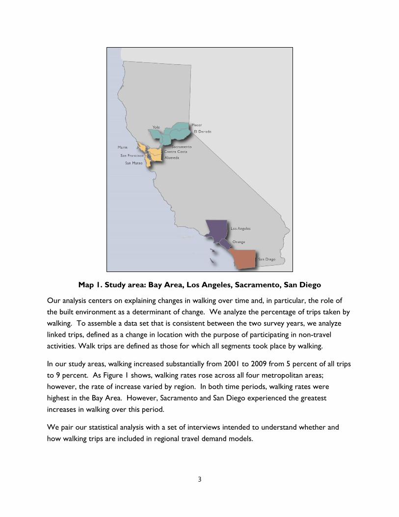
In this report, we extend the existing body of scholarship on walking by analyzing data from the
2001 and 2012 California Household Travel Survey (CHTS), a sample of some 42,000
households in the state. We examine walking in the four largest urbanized regions—the Bay
Area, Los Angeles, Sacramento, and San Diego—areas that comprise approximately 60 percent
of the state’s population. See Map 1 for the location of our study area.
3
Map 1. Study area: Bay Area, Los Angeles, Sacramento, San Diego
Our analysis centers on explaining changes in walking over time and, in particular, the role of
the built environment as a determinant of change. We analyze the percentage of trips taken by
walking. To assemble a data set that is consistent between the two survey years, we analyze
linked trips, defined as a change in location with the purpose of participating in non-travel
activities. Walk trips are defined as those for which all segments took place by walking.
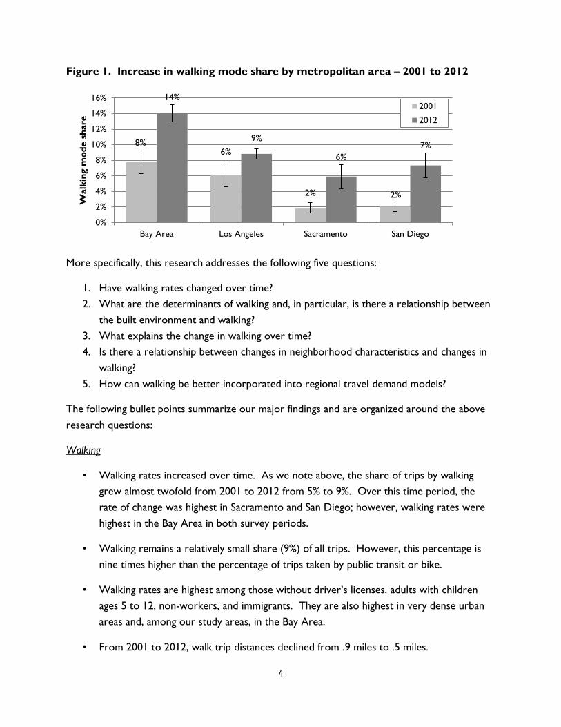
In our study areas, walking increased substantially from 2001 to 2009 from 5 percent of all trips
to 9 percent. As Figure 1 shows, walking rates rose across all four metropolitan areas;
however, the rate of increase varied by region. In both time periods, walking rates were
highest in the Bay Area. However, Sacramento and San Diego experienced the greatest
increases in walking over this period.
We pair our statistical analysis with a set of interviews intended to understand whether and
how walking trips are included in regional travel demand models.
4
Figure 1. Increase in walking mode share by metropolitan area – 2001 to 2012
More specifically, this research addresses the following five questions:
1. Have walking rates changed over time?
2. What are the determinants of walking and, in particular, is there a relationship between
the built environment and walking?
3. What explains the change in walking over time?
4. Is there a relationship between changes in neighborhood characteristics and changes in
walking?
5. How can walking be better incorporated into regional travel demand models?
The following bullet points summarize our major findings and are organized around the above
research questions:
Walking
• Walking rates increased over time. As we note above, the share of trips by walking
grew almost twofold from 2001 to 2012 from 5% to 9%. Over this time period, the
rate of change was highest in Sacramento and San Diego; however, walking rates were
highest in the Bay Area in both survey periods.
• Walking remains a relatively small share (9%) of all trips. However, this percentage is
nine times higher than the percentage of trips taken by public transit or bike.
• Walking rates are highest among those without driver’s licenses, adults with children
ages 5 to 12, non-workers, and immigrants. They are also highest in very dense urban
areas and, among our study areas, in the Bay Area.
• From 2001 to 2012, walk trip distances declined from .9 miles to .5 miles.
8%6%
2% 2%
14%
9%
6%
7%
0%
2%
4%
6%
8%
10%
12%
14%
16%
Bay Area Los Angeles Sacramento San Diego
Walk
ing m
od
e s
hare
2001
2012

5
• The 2012 travel survey is large and appears to have captured a significant number of
walk trips. In comparison, however, the sample of walk trips in the 2001 survey is
relatively small. Moreover, trip data in the two surveys were assembled differently,
complicating analyses of change over time.
Determinants of Walking
• Like other studies, we find that walking can be explained by a number of different
factors including characteristics of the individual, household, trip, and the built
environment as well as geographic location (in this case, residential location in one of
the four metropolitan areas in our study).
• There is a positive and statistically-significant relationship between walking and the built
environment.
• The built environment has a relatively small effect on walking compared to other factors
such as individual, household, and trip characteristics (e.g. distance and purpose). Trip
distance is a function of having proximate destinations and is therefore related to the
built environment.
• Factors with a strong association with walking include: trip distance, trip purpose
(particularly for home-based fitness trips), and the absence of a driver’s license.
Explanations for the Change in Walking over Time
• Observed changes in the built environment are positively associated with changes in
walk rates over time.
• There are two types of built environment effects: (a) changes in the characteristics of
the built environment toward environments conducive to walking and (b) changes in the
effect of the built environment on the likelihood of walking.
• Characteristics of the neighborhood (density, age of housing stock, percent youth) are
associated with walking. The magnitude of their effects has remained constant over
time.
• Neighborhood characteristics have a relatively small effect on changes in walking
compared to other factors such as (a) individual, household, and trip characteristics and
(b) changes in the magnitude of their effect on walking.
• Trip characteristics (trip distance and purpose) have the greatest effect on the likelihood
of walking; the magnitude of these effects has increased over time.

6
• There is a lack of built environment data by neighborhood over time. Consequently,
the analysis relies on a limited set of neighborhood characteristics included in the U.S.
Census.
Changes in Neighborhood Characteristics and Changes in Walking
• Changes in neighborhood characteristics are associated with changes in walking.
• The poverty rate is negatively related to walking; an increase in poverty is associated
with a decline in walking mode share.
• Intersection density is positively related to walking; an increase in the number of
intersections per acre is associated with an increase in walking mode share.
• The ability to construct longitudinal analyses of walking is limited by the small sample
size of the 2001 household travel survey as well as the lack of built environment data by
neighborhood over time.
Walking and Regional Travel Demand Models
• Most of the Metropolitan Planning Organizations (MPOs) that are responsible for
regional transportation planning within our study areas have shifted to activity-based
models, which are better suited to understanding walking compared to the traditional 4-
step model.
• Notable issues and gaps still exist including (a) a mismatch between the goals of travel
demand models (largely focused on the supply and demand for travel as represented by
the highway and transit network) and walking and (b) the lack of high quality,
longitudinal data on the pedestrian volumes, flows and the pedestrian environment,
sidewalks specifically.
The analysis has a few shortcomings that are important to note. First, there are some data
limitations that constrained our analysis including a relatively small sample size in 2001,
inconsistencies in the reporting of walk trips between the two survey years, and the lack of
longitudinal data on the built environment of neighborhoods. Second, there is a self-selection
bias related to residential location. Some respondents who are inclined to walk also may be
more likely to live in “walkable neighborhoods.” Studies show that controlling for residential
self-selection tends to diminish, but not eliminate, estimates of the effects of the built
environment on travel behavior (Cao et al., 2006; Ewing & Cervero, 2010; Handy, Cao, &

7
Mokhtarian, 2005; Mokhtarian & Cao, 2008; Zhou & Kockelman, 2008). Further, Levine et al.
(2005) argue that residential self-selection is one of the means by which the built environment
can influence travel behavior, especially if particular types of built environments are
undersupplied. Finally, while we find a relatively small relationship between the built
environment and walking, travel distance has a strong effect on walking and also is strongly
associated with characteristics of the built environment, particularly local access to
opportunities.
The findings of this study suggest the following recommendations, which we highlight in greater
detail in the conclusion in each of the subsequent chapters.
1. The data suggest that planners can facilitate walking by emphasizing increased
intersection densities and providing better pedestrian route directness. However,
substantial increases in walking can only occur with equally substantial changes in the
built environment.
2. Changes in the built environment targeted to population groups that already exhibit
relatively high rates of walking also may increase walking. These changes might include
addressing safety and crime issues in low-income neighborhoods where a
disproportionate number of households do not own automobiles. They may also
involve improving the proximity of family- and child-oriented amenities, such as high-
quality schools and childcare facilities, which may increase opportunities for walking by
members of households with young children, who are already more inclined to walk
than their peers.
3. Walk trips tend to be short. Therefore, planning efforts to provide very local access
(within a ½ mile) to important destinations (e.g. parks, fitness venues, schools, cultural
institutions, etc.) would increase the likelihood that some of these trips are taken on
foot.
4. Additional data are needed on (a) walking behavior, (b) pedestrian volumes and location,
and (c) the pedestrian environment over time to support future analyses of travel
behavior as well as regional travel models. Larger sample sizes are important,
particularly since a relatively small percentage of trips are walk trips. Moreover, the
data ought to be collected and assembled consistently over time to facilitate longitudinal
analyses.
We organize this report as a set of separate analytical chapters. In Chapter Two, we analyze
data from the 2012 CHTS to examine the relationship between walking and the built
environment. Working with the most recent data allows us to associate the microdata data
8
(data on trips and the individuals who make them) with a full complement of built environment
characteristics (including data on the pedestrian environment from Walk Score®).1 In Chapter
Three, we aggregate data from the two travel surveys to examine the determinants of change in
walking over time. In Chapter Four, we shift the unit of analysis from the trip to the census
tract. In this chapter we explore the relationship between changes in the characteristics of
census tracts and changes in walk rates over time. Finally, in Chapter Five, we report on the
findings from our interviews with planners and regional travel demand modelers. Each chapter
includes an associated literature review, discussion of methodology, and a set of policy
recommendations.2 Additional analyses and data including tables and maps by region and county
are included in the Appendices.
1Data provided by Redfin Real Estate https://www.redfin.com
2This report structure helps to explain why the content of the literature review in each of the analytical chapters
overlaps.

9
References
Agrawal, A. W., Schlossberg, M., & Irvin, K. (2008). How Far, by Which Route and Why? A
Spatial Analysis of Pedestrian Preference. Journal of Urban Design, 13(1), 81–98.
http://doi.org/10.1080/13574800701804074
Agrawal, A. W., Schlossberg, M., & Irvin, K. (2008). How Far, by Which Route and Why? A
Spatial Analysis of Pedestrian Preference. Journal of Urban Design, 13(1), 81–98.
http://doi.org/10.1080/13574800701804074
Badland, H., & Schofield, G. (2005). Transport, Urban Design and Physical Activity: An Evidence-
Based Update. Transportation Research Part D, 10, 177–196.
Blumenberg, E., Brown, A., Ralph, K., Taylor, B. D., & Turley Voulgaris. (2015). Typecasting
Neighborhoods and Travelers. Analyzing the Geography of Travel Behavior among Teens and Young
Adults in the U.S. University of California Los Angeles: Institute of Transportation Studies,
University of California, Los Angeles.
Cao, X., Handy, S., & Mokhtarian, P. L. (2006). The Influences of the Built Environment and
Residential Self-Selection on Pedestrian Behavior: Evidence from Austin, TX. Transportation,
33(1), 1–20. http://doi.org/10.1007/s11116-005-7027-2
Cervero, R., & Duncan, M. (2003). Walking, Bicycling, and Urban Landscapes: Evidence From
the San Francisco Bay Area. American Journal of Public Health, 93(9), 1478–1483.
http://doi.org/10.2105/AJPH.93.9.1478
Cervero, R., & Radisch, C. (1996). Travel Choices in Pedestrian Versus Automobile Oriented
Neighborhoods. Transport Policy, 3(3), 127–141. http://doi.org/10.1016/0967-070X(96)00016-9
Clifton, K. J., & Krizek, K. J. (2004). The Utility of the NHTS In Understanding Bicycle and
Pedestrian Travel (pp. 1–2). Presented at the National Household Travel Survey Conference:
understanding our nation’s travel.
Forsyth, A., Michael Oakes, J., Lee, B., & Schmitz, K. H. (2009). The Built Environment, Walking,
and Physical Activity: Is the Environment More Important to Some People Than Others?
Transportation Research Part D: Transport and Environment, 14(1), 42–49.
http://doi.org/10.1016/j.trd.2008.10.003
Forsyth, A., Hearst, M., Oakes, J. M., & Schmitz, K. H. (2008). Design and Destinations: Factors
Influencing Walking and Total Physical Activity. Urban Studies, 45(9), 1973–1996.
http://doi.org/10.1177/0042098008093386

10
Forsyth, A., Oakes, J. M., Schmitz, K. H., & Hearst, M. (2007). Does Residential Density Increase
Walking and Other Physical Activity? Urban Studies, 44(4), 679–697.
http://doi.org/10.1080/00420980601184729
Frank, L. D., Kerr, J., Sallis, J. F., Miles, R., & Chapman, J. (2008). A Hierarchy of
Sociodemographic and Environmental Correlates of Walking and Obesity. Preventive Medicine,
47(2), 172–178. http://doi.org/10.1016/j.ypmed.2008.04.004
Guerra, E., Cervero, R., & Tischler, D. (2012). Half-Mile Circle. Transportation Research Record:
Journal of the Transportation Research Board, 2276, 101–109. http://doi.org/10.3141/2276-12
Handy, S. (2005). Smart Growth and the Transportation-Land Use Connection: What Does the
Research Tell Us? International Regional Science Review, 28(2), 146–167.
http://doi.org/10.1177/0160017604273626
Handy, S., & Clifton, K. J. (2001). Local Shopping As a Strategy for Reducing Automobile Travel.
Transportation, 28, 317–346.
Krizek, K. J., Handy, S. L., & Forsyth, A. (2009). Explaining Changes in Walking and Bicycling
Behavior: Challenges For Transportation Research. Environment and Planning B: Planning and
Design, 36, 725–740.
Kuzmyak, J., Baber, C., & Savory, D. (2006). Use of Walk Opportunities Index to Quantify Local
Accessibility. Transportation Research Record: Journal of the Transportation Research Board, 1977,
145–153. http://doi.org/10.3141/1977-19
Lachapelle, U., & Noland, R. B. (2012). Does the Commute Mode Affect the Frequency of
Walking Behavior? The Public Transit Link. Transport Policy, 21, 26–36.
http://doi.org/10.1016/j.tranpol.2012.01.008
Lin, L., & Moudon, A. V. (2010). Objective Versus Subjective Measures of the Built Environment,
Which are Most Effective in Capturing Associations with Walking? Health & Place, 16(2), 339–
348. http://doi.org/10.1016/j.healthplace.2009.11.002
Moudon, A. V., Lee, C., Cheadle, A. D., Garvin, C., Johnson, D. B., Schmid, T. L., & Weathers,
R. D. (2007). Attributes of Environments Supporting Walking. American Journal of Health
Promotion, 21(5), 448–459. http://doi.org/10.4278/0890-1171-21.5.448
Oakes, J. M., Forsyth, A., & Schmitz, K. H. (2007). The Effects of Neighborhood Density and
Street Connectivity on Walking Behavior: The Twin Cities Walking Study. Epidemiologic
Perspectives & Innovations : EP+I, 4, 16. http://doi.org/10.1186/1742-5573-4-16

11
Owen, N., Humpel, N., Leslie, E., Bauman, A., & Sallis, J. F. (2004). Understanding Environmental
Influences on Walking: Review and Research Agenda. American Journal of Preventive Medicine,
27(1), 67–76. http://doi.org/10.1016/j.amepre.2004.03.006
Plaut, P. O. (2005). Non-Motorized Commuting in the US. Transportation Research Part D:
Transport and Environment, 10(5), 347–356. http://doi.org/10.1016/j.trd.2005.04.002
Ralph, K., Turley Voulgaris, C., Taylor, B. D., Blumenberg, E., & Brown, A. (2016). Youth,
Travel, and the Built Environment: Insights from Typecasting Places and Younger Travelers.
Presented at the Transportation Research Board 95th Annual Meeting. Retrieved from
https://trid.trb.org/view.aspx?id=1393735
Saelens, B. E., & Handy, S. L. (2008). Built Environment Correlates of Walking: A Review.
Medicine and Science in Sports and Exercise, 40(7 Suppl), S550–S566.
http://doi.org/10.1249/MSS.0b013e31817c67a4
Saelens, B. E., Sallis, J. F., & Frank, L. D. (2003). Environmental Correlates of Walking and
Cycling: Findings from the Transportation, Urban Design, And Planning Literatures. Annals of
Behavioral Medicine, 25(2), 80–91. http://doi.org/10.1207/S15324796ABM2502_03
Santos, A., McGuckin, H., Nakamoto, Gray, D., & Liss, S. (2011). Summary of Travel Trends: 2009
National Household Travel Survey (Trends in Travel Behavior, 1969-2009 No. FHWA-PL-11-022).
Washington, D.C.: US Department of Transportation.
Voulgaris, C. T., Taylor, B. D., Blumenberg, E., Brown, A., & Ralph, K. (Forthcoming).
Neighborhood Character and Travel Behavior: A Comprehensive Analysis of the U.S. Journal of
Transport and Land Use.
Yang, Y., & Diez-Roux, A. V. (2012). Walking Distance by Trip Purpose and Population
Subgroups. American Journal of Preventative Medicine, 43(1), 11–19.
12
II. Are these streets made for walking? Walking and the built environment in
California
Introduction
Planners, environmentalists and public health officials hope that by refashioning America’s
roadways to encourage pedestrian activity, cities will experience a plethora of social and
environmental benefits. Their premise is that cities where more people walk to complete their
daily activities will be full of healthy people, thriving businesses and socially-connected
neighborhoods. Although it is difficult to isolate causality, a growing body of research shows
relationships between walking and pedestrian-friendly neighborhoods and a number of
outcomes measures including lower obesity rates (Frank et al., 2004; Murphy et al., 2007),
higher property values (Pivo & Fisher, 2011; Rauterkus & Miller, 2011), increased social capital
(Leyden, 2003; Rogers et al., 2011), improved quality of life (Talen 2002; Jaśkiewicz & Besta,
2014), and better access to opportunities (Cerin et al., 2007).
Given the many purported benefits of walking, urban planners have championed “walkability”
through a variety of infrastructure projects and initiatives. The names, Great Streets, Safe
Streets, Complete Streets, and so on, convey the enthusiasm of planners for creating more
walkable neighborhoods. However, specific definitions of and measures of walkability are
needed if we are to evaluate the success of these efforts. While there is no shortage of possible
measures of walkability — the search for a single walkability measure is frustrated both by the
multi-dimensional character of the built environment and a lack of readily available built
environment data for all possible scopes (e.g. for national, regional, or local studies), scales (e.g.
with data measured at the city, neighborhood, or parcel level), and time periods.
The purpose of this analysis is to identify the relationships between several walkability measures
and to determine the degree to which such measures predict the likelihood of walking. We
draw on data from the 2012 California Household Travel Survey to determine how walking
varies within California’s four major metropolitan areas —the Bay Area, Los Angeles,
Sacramento, and San Diego— and compare this distribution to that of various measures that
have been proposed by researchers to quantify walking behavior. We then estimate a logistic
regression model to determine how well these measures of the built environment predict the
likelihood that a trip will take place by walking, controlling for trip, individual, and household
characteristics.
Our analysis is organized as follows. We first examine existing research on the factors
influencing travel behavior generally and the choice to walk more specifically. Following this
review, we present descriptive statistics on differences in walking across urban areas and

13
neighborhood types. As might be expected, there is more walking in the San Francisco region
and in “old urban” areas, neighborhoods with very high-densities and transit supply. We then
estimate a trip-level model to identify the factors related to the likelihood a trip will be
completed by walking, controlling for individual, household, trip, and built environment
characteristics and geographic location (e.g. metropolitan area).
Our findings suggest that all these factors influence the choice to walk. However, individual,
household and regional variables influence the choice to walk to a much greater degree than
built environment factors, a finding consistent with other research on this topic. We suggest
policymakers, planners and engineers recognize some groups are more likely to take walk trips
than others and consider prioritizing areas where these people live for improvements to the
walking environment.
Literature review: Walking and the built environment
Neighborhood and built environment characteristics influence travel decisions and behavior. In
their meta-analysis of existing literature on this topic, Ewing and Cervero (2010) find that built
environment variables have an inelastic relationship with most travel outcomes. With respect
to walking behavior, the variables with the largest effects include diversity of land use, access to
destinations and intersection density. Nevertheless, they conclude that in concert, multiple built
environment variables may exhibit large effects on walking behavior even after accounting for
socio-demographic characteristics. Their analysis builds on several previous studies which
consider the individual and sometimes overlapping components of the built environment that
affect travel behavior, such as density, diversity (of land use), design, destination accessibility,
distance to transit, and pedestrian amenities (An & Chen 2009; Cervero & Kockelman, 1997;
Ewing & Cervero, 2001, 2010; Ewing & Handy, 2009; Mathews et al., 2009).
The goal in studying each of these individual components is to determine which environmental
aspects encourage or dissuade walking. In some cases, specific measures—employment density,
residential density, or distance to commercial businesses—serve as proxies for these
dimensions. We briefly discuss these measures in turn below.
Density
Many studies report a strong positive correlation between various measures of density and
walking outcomes: population density (Agrawal & Schimek, 2007; Forsyth et al., 2008;
Greenwald & Boarnet, 2001; Kim & Susilo, 2013); employment density (An & Chen, 2009;
Wang, 2012); and residential density (Rajamani et al., 2003). The relationship between density
and walking behavior is likely nonlinear (Christiansen et al., 2016). Density of a certain

14
magnitude may provide, what Forsyth et al. (2008) refer to as, a “critical mass” to energize
street life with people walking. But, critical density is unlikely achieved without many of the
other built environment characteristics also known to encourage walking trips. Therefore,
density variables run the risk of overlapping with other built environment variables, in
particular, proximity to destinations and diversity of land uses. When considering density as a
walking determinant, an aptly mentioned question in Forsyth et al. (2008) asks: “Once this
critical mass of land use variety has been reached, will more mix matter?” Moreover, an
increasing number of destinations, density and diversity of land-use could eventually lead to
diminishing returns (Christiansen et al., 2016). At some threshold, increased density may
produce negative effects such as congestion that may influence affect modal decisions.
Proximity to destinations
Do people walk more when there are nearby places to go? In California, more than 25 percent
of California Household Travel Survey respondents reported that the greatest barrier to
walking was having “no place interesting to go” (McGuckin, 2012). Thus, it would seem likely
that increased proximity to desirable places (shopping, restaurants, parks, etc.) would motivate
individuals to make more walking trips. This assumption is supported by many scholars who find
a relationship between walking trip frequency, population density and destination proximity
(Handy et al., 2006; Kim & Susilo, 2013; McGuckin, 2012; Saelens & Handy, 2008). These factors
are likely interrelated: proximity to destinations increases with density and vice versa (Saelens &
Handy, 2008). Perceived proximity may also affect walking. Handy et al. (2006) find a positive
correlation between both perceived and objective proximity to destinations and walking.
Proximity to certain types of destinations may matter more than others. Are people more
likely to walk to a nearby transit stop than to school? Some studies examine the relationship
between walking and proximity to shopping districts (as well as the spatial distribution and
number of shopping destinations within an area). However, existing research does not address
which destination types are most strongly correlated with walk trips.
Diversity of land use
Areas with higher density and more proximate locations likely have a more diverse mix of land
uses; therefore, the mix of land uses may also be relevant in the relationship between walking
frequency and density (Kim & Susilo, 2013). A number of studies find a positive correlation
between mixed-land uses and walking or non-motorized travel (Forsyth et. al., 2008; Kim &
Susilo, 2013; Rajamani et al., 2003).

15
Street connectivity
The connectivity of street networks, or “directness or ease of travel between two points” also
emerges as a feature of the built environment pertinent to walking (Forsyth et al., 2008a-quoted
Saelens et al., 2003). Streets are commonly aligned in a gridiron pattern in older cities and
neighborhoods. This pattern gives rise to smaller blocks, more intersections, and shorter
distances from one intersection to the next. Conversely, newer or suburban environments
typically comprise neighborhoods with branching street networks and intersections. These
street connectivity patterns, or typologies, have been used as a proxy for urban sprawl
(Barrington-Leigh & Millard-Ball, 2015).
Many researchers posit that the number of linkages between streets or connections induce
walking. Wang (2012) measures connectivity as the density of four-way intersections and finds a
positive relationship with non-motorized trips. Ewing and Cervero (2010) find a higher average
elasticity between intersection and street density than other design variables. Interestingly, they
find a negative elasticity associated with percentage of four-way intersections. They note that
this measure of connectivity does not fully account for block length, which they believe explains
the discrepancy. Finally, Oakes et al. (2007) use block size as measure for connectivity and find
an increase in leisure walking with no effect on travel walking. The connectivity results, thus,
appear mixed, although they do represent a worthy attempt to quantify discernable patterns in
urban design.
Barrington-Leigh and Millard-Ball (2015) suggest average nodal degree as a useful measure of
street connectivity and as a proxy for sprawl. Average nodal degree is the average number of
legs at each intersection within an area (such as a census block group or tract). For example,
the end of a cul-de-sac has a nodal degree of one, and a four-legged intersection has a nodal
degree of four3. Neighborhoods with the highest average nodal degree are those with dense
grid networks and few dead-ends.
3See Appendix C for a detailed and graphic representation of this concept.

16
Walkability composite measures
No single measure of the built environment appears to have a predominant or “magical”
influence on people’s choice to walk. Rather, certain characteristics in combination create
places where people are likely to walk. Various researchers have devised or used composite
measures of walkability to capture multiple characteristics of the built environment; these
include Walk Score® (Foti & Waddel, 2014; Manaugh & El Geneidy, 2011; Weinberger & Sweet,
2012), neighborhood typologies (Blumenberg et al., 2015; Voulgaris et al., forthcoming),
walkability index (Frank et al., 2005), and Sprawl Index (Hamadi et al., 2015).
Walk Score® is a commercial product that rates neighborhoods on a scale from 1-100 of
walkability, from “car-dependent” to “walker’s paradise.”4 The algorithm counts destinations
across a number of categories (shopping, culture, dining, etc) by their distance and then
penalizes places with low population density or intersection connectivity. A number of studies
have tested the reliability of Walk Score® and find it to be correlated with components of
neighborhood walkability including street connectivity, access to public transit, and residential
density (Carr et al., 2010; Duncan et al., 2012).
Weinberger and Sweet (2012) find that Walk Score® is a reasonable predictor of walking
behavior, and can successfully be used to model the likelihood of walking across various trip
purposes. Their analysis also suggests that threshold effects exist with respect to Walk Score®;
the largest gains in walking trips occur between Walk Scores® of 50 and 100.
Manaugh and El-Geneidy (2011) compared multiple walkability indices, including Walk Score®
and walkability index, and their effectiveness in predicting walking behavior across various trip
purposes. They find, and are supported by later work by Koschinsky et al. (2016) that
walkability indices have a greater impact on wealthier and larger households. In other words,
elasticities are much higher for these groups, and relatively inelastic for low-income individuals.
This finding is consistent with other research concluding that socioeconomic factors have the
largest influence on a person’s likelihood to make a walk trip (Ewing & Cervero, 2010; Ewing et
al., 2014; Handy & Clifton, 2001). Public health researchers have used Walk Score® to examine
the relationship between walkability and obesity rates (Wasserman et. al, 2014).
4Data were provided by Redfin Real Estate, https://www.redfin.com

17
Blumenberg et al. (2015) and Voulgaris et al. (forthcoming) apply factor analysis and cluster
analysis to develop a categorical composite measure of the built environment. They classify
census tracts in the United States into one of seven distinct neighborhood types: Rural, New
Development, Patchwork, Urban Residential, Old Urban, and Mixed Use (or Job Center). Of
these, they find that “New Development” neighborhoods are the most car-dependent and “Old
Urban” neighborhoods are the least car-dependent.
Transportation versus leisure walking
Some environmental features that are conducive to utilitarian walk trips (e.g. proximity to
destinations) may not be conducive to recreational walk trips. For example, Lee and Moudon
(2006) find an inverse relationship between the presence of “hills” and recreational and
utilitarian walking. “Hills” may be related to more walking for recreation but less walking for
transport. Additionally the presence of transit, sidewalks, streetlights and connected land uses
(among others) appear to have negative associations with recreational walking but are positively
related to utilitarian walking (Forsyth et al., 2008). Therefore, trip purpose, at least in terms of
utilitarian versus recreational purposes, should be considered when understanding the
determinants of walking behavior. Other scholars suggest that walking for transportation may
actually replace walking for recreation, an idea referred to in public health and other literature
as an “activity budget” (Forsyth et al., 2008; Oakes et al., 2007). The concept behind the activity
budget is that, as with time, individuals make tradeoffs depending on how much total activity
they deem necessary. A person may forgo their recreational walk around the neighborhood for
a walk to work or school, and vice versa.
Data and descriptive analysis
We draw on the built environment and walking literature in assembling our analysis of walking
in California’s large metro regions. The 2012 California Household Travel Survey (CHTS) is the
primary data source for this study. Conducted by the California Department of Transportation,
the CHTS collects travel data on an approximate ten-year cycle from households throughout
California. Members of participating households completed travel diaries with detailed
information about all trips and activities during a pre-assigned 24-hour period, where dates
were assigned to ensure that data were collected for every day for a full year. Upon completing
the travel diary, survey participants reported their travel through a computer-assisted
telephone interview or by returning the travel diaries by mail.
Our analysis is limited to adult survey respondents living in one of California’s four major
metropolitan areas: the Bay Area (San Francisco, Marin, San Mateo, Contra Costa, and Alameda
counties), Los Angeles (Los Angeles and Orange counties), Sacramento (Sacramento, Placer, El

18
Dorado, and Yolo counties), and San Diego (San Diego county) (see Map 1) . These regions
and their component counties make up more than 60 percent of the state’s population
(California Department of Finance, 2016). Since the study focuses on intra-metropolitan travel,
we exclude from our analysis any trips that were longer than 150 miles.
Also, the study centers on utilitarian trips where the primary mode was walking. Thus, a trip is
defined as a change in location with the purpose of participating in non-travel activities.
However, the 2012 CHTS also includes information on trips with a purpose of changing
transportation modes (walking to a transit station or a remote parking location, for example) as
well as loop trips (for instance, going on a walk for exercise, where the trip begins and ends in
the same location). In order to limit our analysis to utilitarian walk trips, we removed all loop
trips from the data set and linked all mode-changing trips together to identify the trips’ ultimate
origins and destinations. Walk trips are defined as trips for which all segments took place by
walking.
Figure 2 shows how the walking mode share differs by metropolitan region. In this and other
figures throughout this paper, error bars indicate 95-percent confidence intervals. Walking is
highest in the Bay Area (13%) and lowest in Sacramento (5%).
Figure 2. Walking mode share by MSA
For the purposes of this analysis, we defined ten different trip purpose categories, which we
differentiated based on activities at trip origins and destinations. Most of these categories are
self-explanatory. Home-based fitness trips are not loop trips (such as recreational walks or bike
rides that begin and end at home), but rather trips to a location for fitness activities, such as a
gym, a fitness class, or a park. Home-based errands include trips for health care, banking, or
other household business. Home-based shopping trips include trips for both routine shopping
and shopping for major purposes. Home-based social/culture trips include trips for recreation
9% 13% 5% 7%0%
2%
4%
6%
8%
10%
12%
14%
16%
Los Angeles Bay Area Sacramento San Diego
Walk
ing m
od
e s
hare
of
trip
s

19
(except exercise), entertainment, visiting friends, and participation in civic and religious
activities.
Figure 3. Distribution of walk trips and non-walk trips by trip purpose
Walk trips differ from non-walk trips in terms of both trip purpose and trip length. As Figure 3
shows, home-based work trips, home-based errands trips, and trips that do not begin or end at
work or at home are underrepresented among walk trips. Work-based trips, home-based
shopping trips, and home-based fitness trips are overrepresented among walk trips. This
difference is most dramatic for home-based fitness trips. While only four percent of non-
walking trips are home-based fitness trips, this category represents eighteen percent of all walk
trips. With an average trip distance of a half-mile, walk trips are also substantially shorter than
non-walk trips, which are just over six miles long, on average.
12%
7%
24% 25%
12%9%
5% 4%2% 1%
4%
10%
18%20%
16%
7%4%
18%
1% 1%
0%
5%
10%
15%
20%
25%
30%
Sh
are
of
Tri
ps
Non-walk trips Walk trips

20
Figure 4. Differences in individual-level characteristics between walkers and non-
walkers
In addition to these trip-level differences, the 2012 CHTS data also allow us to compare
individual-level characteristics of people who made at least one survey-day walk trip (walkers)
to those who traveled exclusively by other modes on the survey day (non-walkers). On
average, walkers are slightly younger (by about eight months) than non-walkers, but this
difference is not significant at a 95-percent confidence level (remember that our analysis does
not include children). Figure 4 illustrates differences between walkers and non-walkers in terms
of sex, driver’s licensure, employment, disability, and nativity. Perhaps surprisingly, walkers are
about as likely as non-walkers to have a disability. Walkers are more likely than non-walkers to
be female, to be without a driver’s license, not to be employed or looking for work, and to be
foreign-born.
We also compare walking households (those in which at least one household member is a
walker) to non-walking households. The average income of a walking household is about
$78,000 per year. The average income of a non-walking household is higher at about $85,000
per year. However, the median incomes for both walking and non-walking households are
equal: $61,000 per year. The average household size for both walking and non-walking
household is also the same: 2.9 people. However, walking households have fewer vehicles per
driver. Non-walking households have an average of one vehicle per driver, and walking
households have an average of 0.8 vehicles per driver. Furthermore, although walking and non-
walking households are, on average, the same size, the age profile of household members is
48% 52%
7%
93%
65%
5%
31%
94%
3% 3%
73%
27%42%
58%
24%
76%
54%
7%
39%
93%
4% 4%
66%
34%
0%
10%
20%
30%
40%
50%
60%
70%
80%
90%
100%
Sh
are
of
Peo
ple
Non-walker
Walker

21
different. As shown in Figure 5, the youngest person in a walking household is more likely to be
a teen and less likely to be a toddler than the youngest person in a non-walking household.
Figure 5. Youngest household member by walking and non-walking households.
The confidential data from the 2012 CHTS includes the latitude and longitude coordinates for
each trip end. Using these coordinates, we geocoded each trip origin to a census block group.
This allows us to examine possible relationships between walking and the built environment.
For data on the built environment, we turned to three different sources:
Tract neighborhood types (Blumenberg et al., 2015; Voulgaris et al., forthcoming)
Block group5 Walk Score®6
Block group nodal degree (Barrington-Leigh & Millard-Ball 2015)
Figure 6 draws on the neighborhood types developed in Blumenberg et al. (2015) and Voulgaris
et al. (forthcoming) and shows the distribution of both walk trips and non-walk trips by
neighborhood type in our four metropolitan regions. Walk trips are underrepresented in the
three suburban neighborhood types (New Development, Patchwork, and Established Suburb),
and overrepresented in Old Urban and Mixed Use (which we now label as “Job Center”)
neighborhoods. The percentage of total walk trips that originate in Old Urban neighborhoods is
more than twice the share of total non-walk trips that originate in those neighborhoods.
5Walk Score® is a point-based measurement. The score for each block group is based on the population-weighted
center of that block group. 6Data were provided by Redfin Real Estate https://www.redfin.com
2%5%
14%
9%
3%
8%
17%
6%
0%
2%
4%
6%
8%
10%
12%
14%
16%
18%
20%
Youngest household
member is a baby (less
than two years old)
Youngest household
member is a toddler
(two to four years old)
Youngest household
member is a child (five
to twelve years old)
Youngest household
member is a teenager
Sh
are
of
ho
use
ho
lds
Non-walking household
Walking household
22
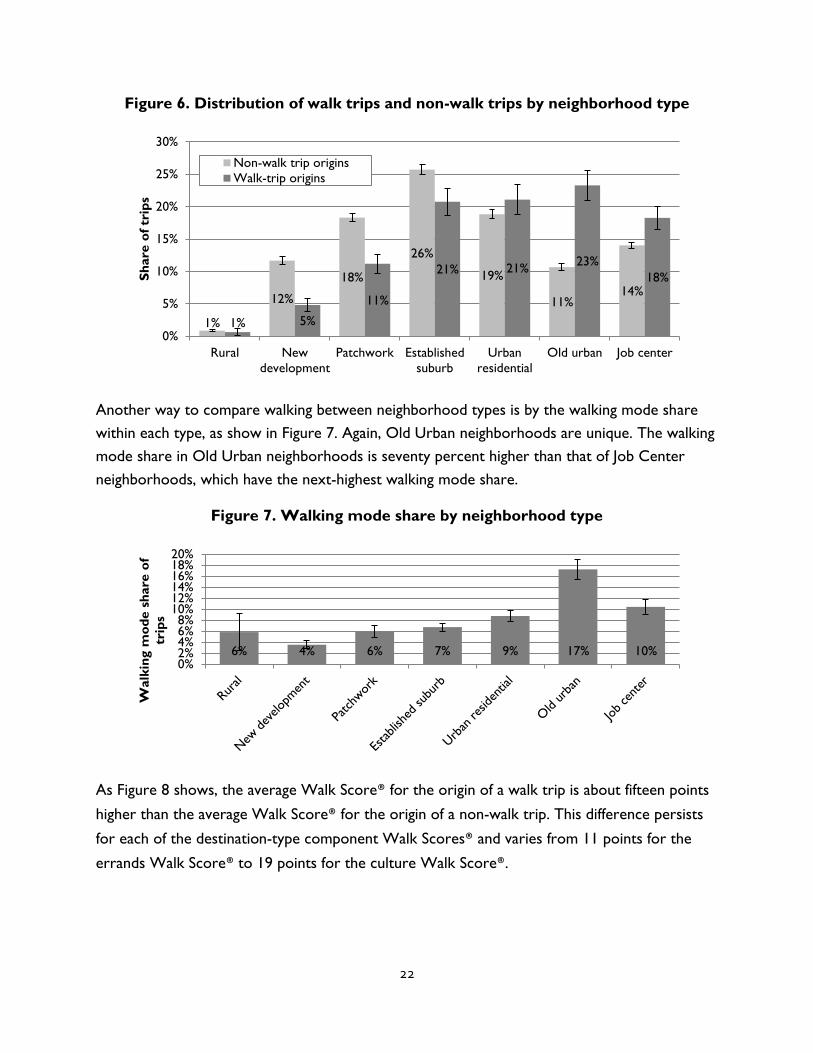
Figure 6. Distribution of walk trips and non-walk trips by neighborhood type
Another way to compare walking between neighborhood types is by the walking mode share
within each type, as show in Figure 7. Again, Old Urban neighborhoods are unique. The walking
mode share in Old Urban neighborhoods is seventy percent higher than that of Job Center
neighborhoods, which have the next-highest walking mode share.
Figure 7. Walking mode share by neighborhood type
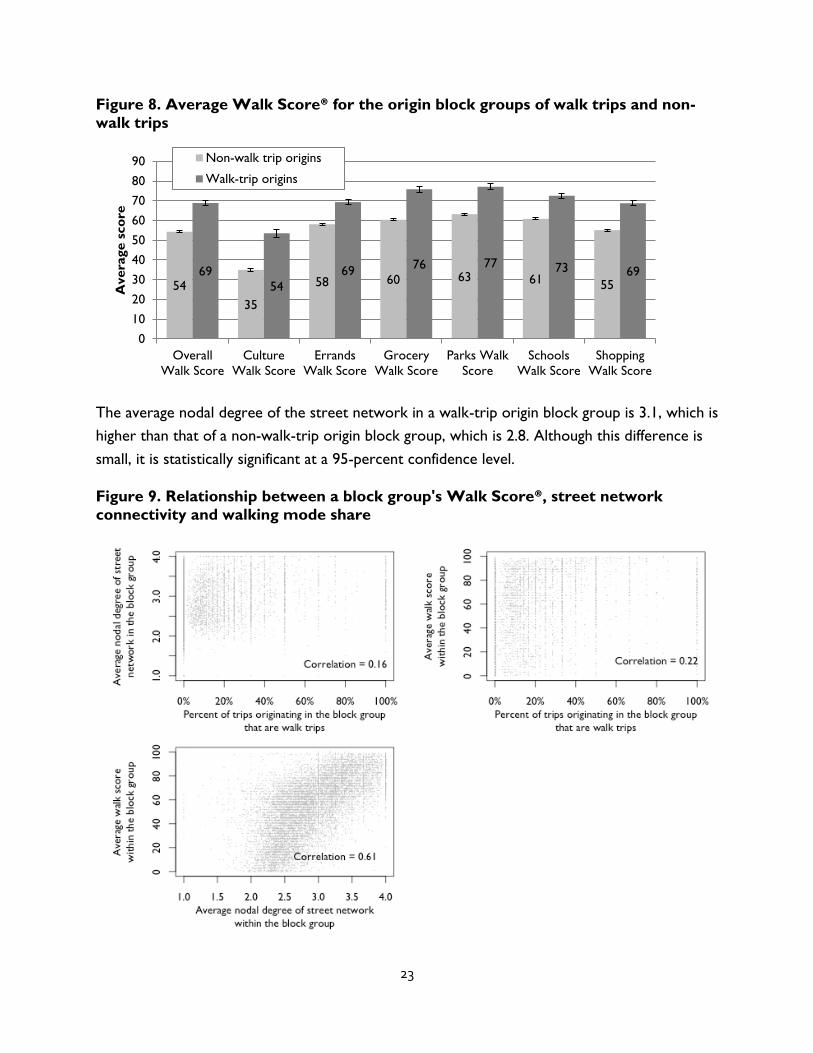
As Figure 8 shows, the average Walk Score® for the origin of a walk trip is about fifteen points
higher than the average Walk Score® for the origin of a non-walk trip. This difference persists
for each of the destination-type component Walk Scores® and varies from 11 points for the
errands Walk Score® to 19 points for the culture Walk Score®.
1%
12%
18%
26%
19%
11%14%
1% 5%
11%
21% 21%23%
18%
0%
5%
10%
15%
20%
25%
30%
Rural New
development
Patchwork Established
suburb
Urban
residential
Old urban Job center
Sh
are
of
trip
s
Non-walk trip origins
Walk-trip origins
6% 4% 6% 7% 9% 17% 10%0%2%4%6%8%
10%12%14%16%18%20%
Walk
ing m
od
e s
hare
of
trip
s
23
Figure 8. Average Walk Score® for the origin block groups of walk trips and non-walk trips
The average nodal degree of the street network in a walk-trip origin block group is 3.1, which is
higher than that of a non-walk-trip origin block group, which is 2.8. Although this difference is
small, it is statistically significant at a 95-percent confidence level.
Figure 9. Relationship between a block group's Walk Score®, street network connectivity and walking mode share
54
35
58 60 63 61 5569
54
6976 77 73 69
0
10
20
30
40
50
60
70
80
90
Overall
Walk Score
Culture
Walk Score
Errands
Walk Score
Grocery
Walk Score
Parks Walk
Score
Schools
Walk Score
Shopping
Walk Score
Avera
ge s
co
re
Non-walk trip origins
Walk-trip origins

24
As shown in Figure 9, there is a positive but weak relationship between a block group’s Walk
Score® and the walking mode share of trips that originate there, and also between the average
street network nodal degree within a block group and the walking mode share of trips that
originate there. Interestingly, Walk Score® and nodal degree are more highly correlated with
one another than either measure is with the walking mode share within a block group.
Figure 10 presents box plots to illustrate how Walk Score® and average nodal degree vary by
neighborhood type. Rural and New Development neighborhoods have the lowest Walk
Scores® and average nodal degree; Old Urban and Job Center neighborhoods have the highest
scores on both measures; and Patchwork, Established Suburb, and Urban Residential
neighborhoods fall somewhere in the middle.
Figure 10. Box plots of variation in Walk Score® and street network connectivity by neighborhood type
Modeling methodology
To better determine the relationship between the built environment characteristics described
above and walking in California’s major metropolitan areas, we incorporated them into a
logistic regression model predicting the likelihood that a particular trip will be a walk trip.
Several prior studies of walking behavior predict mode shares at the person or neighborhood
level.7 Others researchers have modeled mode choice at the trip level, and have found that
trip-level characteristics such as trip length and purpose have important effects on mode
7See, for example, Cao et al. (2006), Forsyth et al. (2007), Forsyth et al. (2009), Joh et al. (2015) and Lee &
Moudon (2006).

25
choice.8 By specifying our model at the trip-level, we are able to control for these trip-level
relationships in our analysis of the relationship between walking and the built environment
Person-level and neighborhood-level models typically analyze built-environment effects on
mode share by estimating relationships between shares of walk trips and the built-environment
characteristics of travelers’ residential locations. However, many trips have origins or
destinations that are outside the traveler’s residential neighborhood. In fact, as shown in Figure
3, about thirty percent of all trips have both an origin and a destination that was not the
traveler’s home. By estimating a trip-level model, we are able to control for the built-
environmental characteristics of trip origins, rather than only characteristics of the traveler’s
residential location.
Table 1 lists the variables that we include in our logistic regression model. We control for
twelve trip, individual, and household characteristics in order to find the independent
relationship between the likelihood of walking and each of three built environment variables.
We estimate three models: the first predicts walking mode choice based only on the MSA
where the traveler lives; the second adds the control variables from Table 1 which describes
trip, individual, and household characteristics; and the third adds the variables describing the
built environment. By comparing the model fit among these models, we can determine the
overall effect of the built environment (as described by Walk Score®, neighborhood type, and
street connectivity) on the odds of walking for a particular trip.
8 See, for example, Cervero & Duncan (2003) and Kockleman (1997).
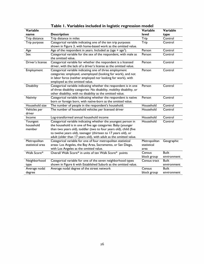
26
Table 1. Variables included in logistic regression model Variable
name Description
Variable
level
Variable
type
Trip distance Trip distance in miles Trip Control
Trip purpose Categorical variable indicating one of the ten trip purposes
shown in Figure 3, with home-based work as the omitted value.
Trip Control
Age Age of the respondent in years. Included as (age + age2). Person Control
Sex Categorical variable for the sex of the respondent, with male as
the omitted value.
Person Control
Driver’s license Categorical variable for whether the respondent is a licensed
driver, with the lack of a driver’s license as the omitted value.
Person Control
Employment Categorical variable indicating one of three employment
categories: employed, unemployed (looking for work), and not
in labor force (neither employed nor looking for work), with
employed as the omitted value.
Person Control
Disability Categorical variable indicating whether the respondent is in one
of three disability categories: No disability, mobility disability, or
other disability, with no disability as the omitted value.
Person Control
Nativity Categorical variable indicating whether the respondent is native
born or foreign born, with native-born as the omitted value.
Person Control
Household size The number of people in the respondent’s household. Household Control
Vehicles per
driver
The number of household vehicles per licensed driver Household Control
Income Log-transformed annual household income Household Control
Youngest
household
member
Categorical variable indicating whether the youngest person in
the household is in one of five age categories: Baby (younger
than two years old), toddler (two to four years old), child (five
to twelve years old), teenager (thirteen to 17 years old), or
adult (older than 17 years old), with adult as the omitted value.
Household Control
Metropolitan
statistical area
Categorical variable for one of four metropolitan statistical
areas: Los Angeles, the Bay Area, Sacramento, or San Diego,
with Los Angeles as the omitted value.
Metropolitan
statistical
area
Geographic
Walk Score® Overall Walk Score® in units of ten Walk Score® points Census
block group
Built
environment
Neighborhood
type
Categorical variable for one of the seven neighborhood types
shown in Figure 6 with Established Suburb as the omitted value.
Census tract Built
environment
Average nodal
degree
Average nodal degree of the street network Census
block group
Built
environment

27
Model results
Table 2 compares the model fit for each of the three models in terms of the Akaike Information
Criterion (AIC) and R2 as well as the coefficients for the MSA indicator variables. The model
explains about one percent of the variation in the decision to walk by MSA alone. When we
include variables describing trip, individual, and household characteristics, the predictive power
of the model increases significantly; this model explains 45 percent of the variation in the
decision to walk. Adding the built environment variables provides an even better fit, but the
difference is relatively minor; the full model explains an additional two percent of the variation
in the decision to walk for a particular trip.
Table 2. MSA effects and logistic regression model fit
Model: MSA only
MSA plus control
variables Full model
Model Fit
AIC 52,848 26,513 25,943
R2 0.01 0.45 0.47
MSA Effects (relative to Los Angeles), 95-percent confidence interval
Bay Area 0.68 – 0.78 0.47 – 0.61 0.40 – 0.55
Sacramento -0.35 – -0.15 -0.42 – -0.16 -0.24 – 0.02
San Diego -0.23 – -0.04 -0.13 – 0.11 -0.02 – 0.23
By comparing the MSA effects from the three models, as shown in Table 2 and illustrated in
Figure 11, we can determine the degree to which the control variables and the built
environment variables each explain differences in walking mode shares among the four MSAs.
The left set of bars in Figure 11 show that the odds that a trip will take place by walking are
greater in the Bay Area and lower in Sacramento and San Diego than in Los Angeles (the odds
that a trip will take place by walking is about the same in Sacramento as in San Diego). This is
consistent with the mode shares shown in Figure 2. The middle set of bars shows that when we
add controls for trip, individual, and household characteristics, the difference between Los
Angeles and San Diego disappears, indicating that this difference can be primarily explained by
non-built-environment characteristics. The right set of bars shows that when we add built
environment characteristics, we have explained most of the difference between San Diego,
Sacramento, and Los Angeles, although the odds of walking continue to be higher in the Bay
Area for reasons that are not included in the model.
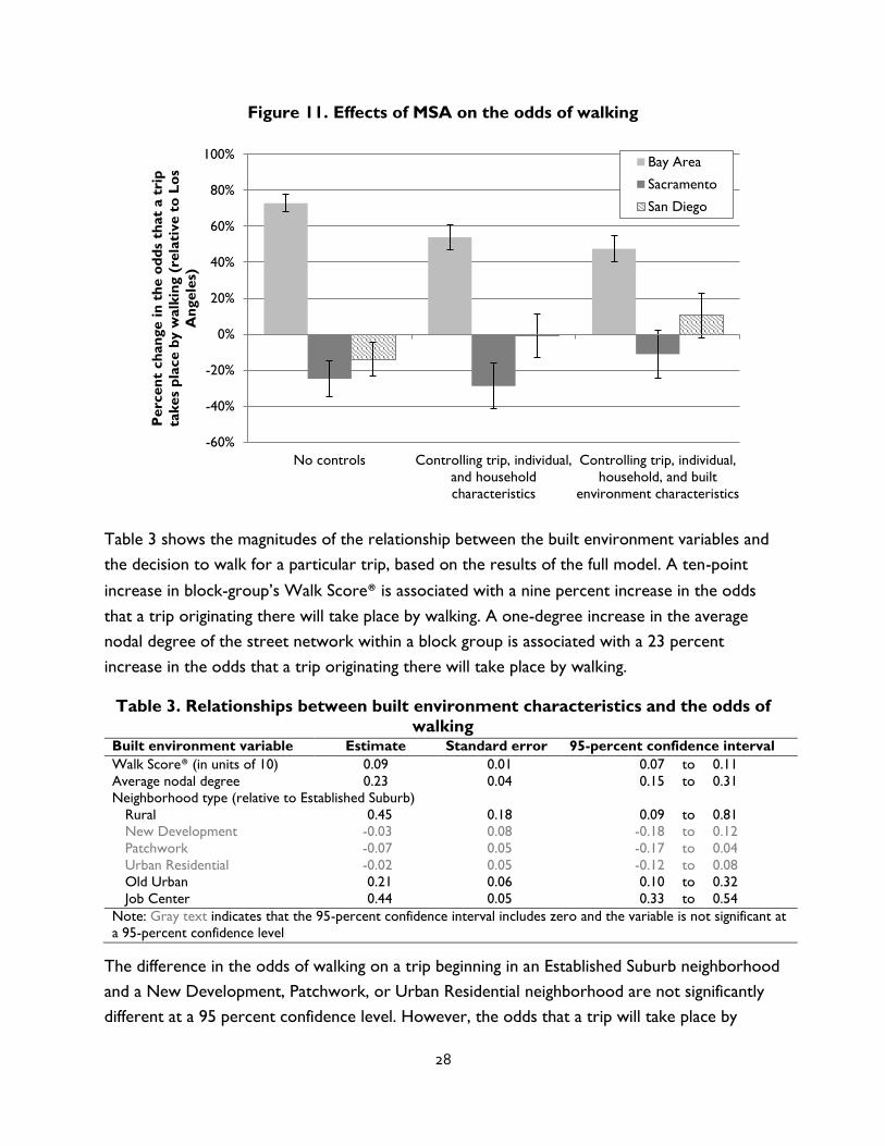
28
Figure 11. Effects of MSA on the odds of walking
Table 3 shows the magnitudes of the relationship between the built environment variables and
the decision to walk for a particular trip, based on the results of the full model. A ten-point
increase in block-group’s Walk Score® is associated with a nine percent increase in the odds
that a trip originating there will take place by walking. A one-degree increase in the average
nodal degree of the street network within a block group is associated with a 23 percent
increase in the odds that a trip originating there will take place by walking.
Table 3. Relationships between built environment characteristics and the odds of
walking Built environment variable Estimate Standard error 95-percent confidence interval
Walk Score® (in units of 10) 0.09 0.01 0.07 to 0.11
Average nodal degree 0.23 0.04 0.15 to 0.31
Neighborhood type (relative to Established Suburb)
Rural 0.45 0.18 0.09 to 0.81
New Development -0.03 0.08 -0.18 to 0.12
Patchwork -0.07 0.05 -0.17 to 0.04
Urban Residential -0.02 0.05 -0.12 to 0.08
Old Urban 0.21 0.06 0.10 to 0.32
Job Center 0.44 0.05 0.33 to 0.54
Note: Gray text indicates that the 95-percent confidence interval includes zero and the variable is not significant at
a 95-percent confidence level
The difference in the odds of walking on a trip beginning in an Established Suburb neighborhood
and a New Development, Patchwork, or Urban Residential neighborhood are not significantly
different at a 95 percent confidence level. However, the odds that a trip will take place by
-60%
-40%
-20%
0%
20%
40%
60%
80%
100%
No controls Controlling trip, individual,
and household
characteristics
Controlling trip, individual,
household, and built
environment characteristics
Perc
en
t ch
an
ge i
n t
he o
dd
s th
at
a t
rip
takes
pla
ce b
y w
alk
ing (
rela
tive t
o L
os
An
gele
s)
Bay Area
Sacramento
San Diego

29
walking is 21 percent greater if it begins in an Old Urban neighborhood and 44 percent greater
if it begins in a Job Center neighborhood than if it begins in an Established Suburb
neighborhood. The high densities and land use diversity within these neighborhood types might
help explain these results. However, trips beginning in Rural neighborhoods are also 45 percent
more likely than trips beginning in Established Suburb neighborhoods to take place by walking,
when we control for Walk Score®, network connectivity, and trip, individual, and household
characteristics. This is consistent with the observations in Figure 7 and Figure 10, which show
that Rural neighborhoods have a moderate walking mode share in spite of having relatively low
Walk Scores® and street network connectivity.
For comparison, Table 4 shows the estimated coefficients for the control variables in the full
model.9 Most of the control variables do have a significant relationship with the odds of walking,
although the magnitudes of these relationships vary substantially. The relationship between trip
distance and the odds that a trip will take place by walking is the most dramatic: a one-mile
reduction in trip distance is associated with a 240 percent increase in the odds that the trip will
take place by walking. A similar increase in the odds of walking are associated with a home-
based fitness trip purpose (207 percent more likely to be a walk trip than a home-based work
trip would be) or with the lack of a driver’s license (177 percent more likely to be a walk trip
than a trip by a person with a driver’s license would be).
9For most control variables, the coefficient estimates in the model that excluded the built environment variables
was within the 95-percent confidence interval of the coefficient estimates in the model that included them (shown
in Table 4). Exceptions were for the non-home-based work trip purpose, household size, and number of vehicles
per driver. The magnitudes of the coefficients for those three variables were greater when built environment
variables were not included in the model.

30
Table 4. Relationships between control variables and the odds of walking Estimate Standard error 95-percent confidence interval
Trip characteristics
Trip distance (miles) -2.40 0.03 -2.47 To -2.34
Trip purpose (relative to home-based work)
Non-home-based work 0.26 0.09 0.09 To 0.42
Other non-home-based -0.78 0.08 -0.93 To -0.63
Home-based errands -0.31 0.08 -0.46 To -0.15
Home-based shopping -0.05 0.08 -0.21 To 0.11
Home-based culture 0.31 0.09 0.14 To 0.48
Home-based dining 0.30 0.10 0.11 to 0.50
Home-based fitness 2.07 0.08 1.90 to 2.23
Home-based school 1.06 0.19 0.69 to 1.43
Home-based other 0.43 0.20 0.05 to 0.82
Individual characteristics
Age 0.03 0.01 0.01 to 0.04
Age squared -3.8x10⁻⁴ 6.5x10⁻⁵ -5.0x10⁻⁴ to -2.5x10⁻⁴
Sex (relative to male)
Female -0.05 0.03 -0.11 to 0.01
Driver’s license (relative to unlicensed)
Licensed -1.77 0.06 -1.89 to -1.64
Employment (relative to employed)
Unemployed 0.14 0.08 -0.01 to 0.29
Not in labor force 0.17 0.04 0.09 to 0.25
Disability (relative to no disability)
Mobility disability -0.68 0.10 -0.88 to -0.47
Other disability -0.75 0.11 -0.96 to -0.53
Nativity (relative to native-born)
Foreign-born 0.10 0.04 0.02 to 0.18
Household characteristics
Household size -0.11 0.02 -0.15 to -0.08
Vehicles per driver -0.82 0.04 -0.90 to -0.73
Income (log-transformed) -0.01 0.02 -0.05 to 0.03
Youngest household member (relative to adult)
Baby 0.28 0.11 0.08 to 0.49
Toddler -0.01 0.08 -0.16 to 0.14
Child -0.05 0.06 -0.16 to 0.06
Teen -0.17 0.07 -0.31 to -0.04
Note: Gray text indicates that the 95-percent confidence interval includes zero and the variable is not significant at
a 95-percent confidence level
31
Discussion
Overall, trip, individual, and household characteristics explain more of the variation in the
decision to walk than do characteristics of the built environment, as shown by the small
increase in model fit that is achieved from adding the built environment variables to the control
variables.
The differences in the odds of walking that can be explained by specific individual characteristics
are also, for the most part greater than the differences explained by specific built environment
characteristics. For example, the difference in the odds of walking associated with having a
driver’s license is four times the difference that would be expected based on a fifty-point
difference in Walk Score®. The difference in the odds of walking for a trip beginning in an
Established Suburb neighborhood (the most common neighborhood type in the study area)
compared to those for a trip beginning in an Old Urban neighborhood (the neighborhood type
with the most walking), would be about the same as the difference between a trip by an
employed person and one by a person who is not in the labor force. A trip by a person with a
disability in a block group with an average nodal degree of about four (a perfect grid network)
as likely to be a walk trip as one by a person with no disability in a block group with an average
nodal degree of about one (where all streets are dead ends).
In fact, holding all of the control variables constant, the greatest difference in the odds of
walking that we would expect to observe based on varying all of the built environment variables
from their minimum possible values to their maximum possible values would be a change of
about 75 percent —the equivalent of reducing a trip’s distance by about a third of a mile.
These findings are consistent with prior studies that suggest that socioeconomic factors have
greater effects on mode choice than characteristics of the built environment (Ewing & Cervero
2010) and that dramatic changes in the built environment are required to achieve moderate
changes in travel behavior. For example, a meta-analysis by Ewing and Cervero (2010) finds that
a doubling in density (measured as population density, employment density, or commercial
floor-area ration) is associated with increases in walking of about seven to four percent; a
doubling of diversity and destination accessibility measures (an entropy index, job-housing
balance, distance between homes and stores, or number of jobs within one mile) is associated
with increases in walking of 15 to 25 percent.

32
Conclusion
Although the built environment has less of an effect on the decision to walk than trip, individual,
and household characteristics, these effects are not unimportant for planners and policy makers
who seek to increase utilitarian walking. In general, planners and policy makers can do little to
influence the individual and household characteristics of travelers (and to the extent that they
can, they probably should not). They do, however, have a variety of tools at their disposal to
facilitate the development of built environments that are conducive to walking. The results of
this study suggest that such tools can have modest but real effects on the choice to walk for a
particular trip.
This study does not assess potential relationships between the built environment and trip
characteristics other than mode. However, such relationships could offer planners and policy-
makers an opportunity to indirectly influence walking mode choice by reducing trip distances,
particularly to destinations that correspond with trip purposes that are associated with greater
odds of walking, such as fitness, culture, school, and dining.

33
References
Agrawal, A. W., & Schimek, P. (2007). Extent and Correlates of Walking in the USA.
Transportation Research Part D: Transport and Environment, 12(8), 548–563.
http://doi.org/10.1016/j.trd.2007.07.005
An, M., & Chen, M. (2007). Estimating Nonmotorized Travel Demand. Transportation Research
Record: Journal of the Transportation Research Board, 2002, 18–25. http://doi.org/10.3141/2002-03
Barrington-Leigh, C., & Millard-Ball, A. (2015). A Century of Sprawl in the United States.
Proceedings of the National Academy of Sciences, 112(27), 8244–8249.
http://doi.org/10.1073/pnas.1504033112
Blumenberg, E., Brown, A., Ralph, K., Taylor, B. D., & Turley Voulgaris. (2015). Typecasting
Neighborhoods and Travelers. Analyzing the Geography of Travel Behavior among Teens and Young
Adults in the U.S. University of California Los Angeles: Institute of Transportation Studies,
University of California, Los Angeles.
California Department of Finance. (2016). Demographic Research. Retrieved June 30, 2016,
from http://www.dof.ca.gov/research/demographic/Estimates/
Cao, X., Handy, S. L., & Mokhtarian, P. L. (2006). The Influences of the Built Environment and
Residential Self-Selection on Pedestrian Behavior: Evidence from Austin, TX. Transportation,
33(1), 1–20. http://doi.org/10.1007/s11116-005-7027-2
Carr, L. J., Dunsiger, S. I., & Marcus, B. H. (2010). Walk Scoretm as a Global Estimate of
Neighborhood Walkability. American Journal of Preventive Medicine, 39(5), 460–463.
http://doi.org/10.1016/j.amepre.2010.07.007
Cerin, E., Leslie, E., du Toit, L., Owen, N., & Frank, L. D. (2007). Destinations that Matter:
Associations with Walking for Transport. Health & Place, 13(3), 713–724.
Cervero, R., & Duncan, M. (2003). Walking, Bicycling, and Urban Landscapes: Evidence From
the San Francisco Bay Area. American Journal of Public Health, 93(9), 1478–1483.
Cervero, R., & Kockelman, K. (1997). Travel demand and the 3Ds: Density, diversity, and
design. Transportation Research Part D: Transport and Environment, 2(3), 199–219.
http://doi.org/10.1016/S1361-9209(97)00009-6

34
Christiansen, L. B., Cerin, E., Badland, H., Kerr, J., Davey, R., Troelsen, J., Van Dyck, D., Mitas, J.,
Schofield, G., Sugiyama, T. (2016). International comparisons of the associations between
objective measures of the built environment and transport-related walking and cycling: IPEN
adult study. Journal of Transport & Health.
Duncan, D. T., Aldstadt, J., Whalen, J., & Melly, S. J. (2012). Validation of Walk Scores and
Transit Scores for Estimating Neighborhood Walkability and Transit Availability: A Small-Area
Analysis. GeoJournal, 78(2), 407–416. http://doi.org/10.1007/s10708-011-9444-4
Ewing, R., & Cervero, R. (2001). Travel and the Built Environment: A Synthesis. Transportation
Research Record: Journal of the Transportation Research Board, 1780, 87–114.
http://doi.org/10.3141/1780-10
Ewing, R., & Cervero, R. (2010). Travel and the Built Environment. Journal of the American
Planning Association, 76(3), 265–294.
Ewing, R., & Handy, S. (2009). Measuring the Unmeasurable: Urban design Qualities Related to
Walkability. Journal of Urban Design, 14(1), 65–84.
Ewing, R., Tian, G., Goates, J. P., Zhang, M., Greenwald, M. J., Joyce, A., Kircher, J., & Greene,
W. (2014). Varying Influences of the Built Environment on Household Travel In 15 Diverse
Regions Of The United States. Urban Studies, 42098014560991.
http://doi.org/10.1177/0042098014560991
Forsyth, A., Hearst, M., Oakes, J. M., & Schmitz, K. H. (2008). Design and Destinations: Factors
Influencing Walking and Total Physical Activity. Urban Studies, 45(9), 1973–1996.
http://doi.org/10.1177/0042098008093386
Forsyth, A., Michael Oakes, J., Lee, B., & Schmitz, K. H. (2009). The Built Environment, Walking,
and Physical Activity: Is the Environment More Important to Some People than Others?
Transportation Research Part D: Transport and Environment, 14(1), 42–49.
http://doi.org/10.1016/j.trd.2008.10.003
Forsyth, A., Oakes, J. M., Schmitz, K. H., & Hearst, M. (2007). Does Residential Density Increase
Walking and Other Physical Activity? Urban Studies, 44(4), 679–697.
http://doi.org/10.1080/00420980601184729
Foti, F., & Waddell, P. (2014). Modeling Walk Trips Using a Multi-modal Accessibility
Framework. Presented at the 93rd Annual Meeting of the Transportation Research Board.
35
Frank, L. D., Andresen, M. A., & Schmid, T. L. (2004). Obesity Relationships with Community
Design, Physical Activity, and Time Spent in Cars. American Journal of Preventive Medicine, 27(2),
87–96.
Frank, L. D., Schmid, T. L., Sallis, J. F., Chapman, J., & Saelens, B. E. (2005). Linking Objectively
Measured Physical Activity with Objectively Measured Urban Form: Findings from SMARTRAQ.
Active Living Research, 28(2, Supplement 2), 117–125.
http://doi.org/10.1016/j.amepre.2004.11.001
Greenwald, M., & Boarnet, M. (2001). Built Environment as Determinant of Walking Behavior:
Analyzing Non-work Pedestrian Travel in Portland, Oregon. Transportation Research Record:
Journal of the Transportation Research Board, 1780, 33–41. http://doi.org/10.3141/1780-05
Hamidi, S., Ewing, R., Preuss, I., & Dodds, A. (2015). Measuring Sprawl and Its Impacts: An
Update. Journal of Planning Education and Research, 35(1), 35–50.
http://doi.org/10.1177/0739456X14565247
Handy, S. (2005). Smart Growth and the Transportation-Land Use Connection: What Does the
Research Tell Us? International Regional Science Review, 28(2), 146–167.
http://doi.org/10.1177/0160017604273626
Handy, S., Cao, X., & Mokhtarian, P. L. (2006). Self-Selection in the Relationship between the
Built Environment and Walking: Empirical Evidence from Northern California. Journal of the
American Planning Association, 72(1), 55–74.
Handy, S., & Clifton, K. J. (2001). Local Shopping as a Strategy For Reducing Automobile Travel.
Transportation, 28, 317–346.
Jaśkiewicz, M., & Besta, T. (2014). Is Easy Access Related to Better Life? Walkability and
Overlapping of Personal and Communal Identity as Predictors of Quality of Life. Applied
Research in Quality of Life, 9(3), 505–516.
Joh, K., Chakrabarti, S., Boarnet, M. G., & Woo, A. (2015). The Walking Renaissance: A
Longitudinal Analysis of Walking Travel in the Greater Los Angeles Area, USA. Sustainability,
7(7), 8985–9011.
Kim, N. S., & Susilo, Y. O. (2013). Comparison of Pedestrian Trip Generation Models. Journal of
Advanced Transportation, 47, 399–412.

36
Kockelman, K. (1997). Travel Behavior as Function of Accessibility, Land Use Mixing, and Land
Use Balance: Evidence from San Francisco Bay Area. Transportation Research Record: Journal of the
Transportation Research Board, 1607, 116–125. http://doi.org/10.3141/1607-16
Koschinsky, J., Talen, E., Alfonzo, M., & Lee, S. (2016). How Walkable is Walker’s paradise?
Environment and Planning B: Planning and Design, 265813515625641.
http://doi.org/10.1177/0265813515625641
Lee, C., & Moudon, A. V. (2006). Correlates of Walking for Transportation or Recreation
Purposes. Journal of Physical Activity and Health, 3(Suppl 1), S77–S98.
Leyden, K. M. (2003). Social Capital and the Built Environment: The Importance of Walkable
Neighborhoods. American Journal of Public Health, 93(9), 1546–1551.
Manaugh, K., & El-Geneidy, A. (2011). Validating Walkability Indices: How Do Different
Households Respond to the Walkability of Their Neighborhood? Transportation Research Part D:
Transport and Environment, 16(4), 309–315.
Mathews, A., E., Colabianchi, N., Hutto, B., Pluto, D., M., & Hooker, S., P. (2009). Pedestrian
Activity Among California Adults. Journal of Physical Activity and Health, 6(1), pp 15-23.
McGuckin, N. (2012). Walking and Biking in California: Analysis of the CA-NHTS (Research Report
No. UCD-ITS-RR-12-13) (pp. 1–36). Davis, CA: Institute of Transportation Studies, University
of California, Davis.
Murphy, M. H., Nevill, A. M., Murtagh, E. M., & Holder, R. L. (2007). The Effect of Walking on
Fitness, Fatness and Resting Blood Pressure: A Meta-Analysis of Randomised, Controlled Trials.
Preventive Medicine, 44(5), 377–385. http://doi.org/10.1016/j.ypmed.2006.12.008
Oakes, J. M., Forsyth, A., & Schmitz, K. H. (2007). The Effects of Neighborhood Density and
Street Connectivity on Walking Behavior: The Twin Cities Walking Study. Epidemiologic
Perspectives & Innovations : EP+I, 4, 16. http://doi.org/10.1186/1742-5573-4-16
Pivo, G., & Fisher, J. D. (2011). The Walkability Premium in Commercial Real Estate
Investments. Real Estate Economics, 39(2), 185–219.
Rajamani, J., Bhat, C., Handy, S., Knaap, G., & Song, Y. (2003). Assessing Impact of Urban Form
Measures on Non-work Trip Mode Choice After Controlling for Demographic and Level-of-
Service Effects. Transportation Research Record: Journal of the Transportation Research Board, 1831,
158–165. http://doi.org/10.3141/1831-18
37
Rauterkus, S. Y., & Miller, N. (2011). Residential Land Values and Walkability. Journal of
Sustainable Real Estate, 3(1), 23–43.
Rogers, S. H., Halstead, J. M., Gardner, K. H., & Carlson, C. H. (2011). Examining Walkability
and Social Capital as Indicators of Quality of Life at the Municipal and Neighborhood Scales.
Applied Research in Quality of Life, 6(2), 201–213.
Saelens, B. E., & Handy, S. L. (2008). Built Environment Correlates of Walking: A Review.
Medicine and Science in Sports and Exercise., 40(7 Suppl), S550–S566.
Talen, E. (2002). Pedestrian Access as a Measure of Urban Quality. Planning Practice and
Research, 17(3), 257–278.
Voulgaris, C. T., Taylor, B. D., Blumenberg, E., Brown, A., & Ralph, K. (Forthcoming).
Neighborhood Character and Travel Behavior: A Comprehensive Analysis of the U.S. Journal of
Transport and Land Use.
Wang, K. (2012, November 15). Causality between the Built Environment and Travel Behavior: A
Structural Equations Model Applied to Southern California. Irvine, CA.
Wasserman, J., Suminski, R., Xi, J., Mayfield, C., Glaros, A., & Magie, R. (2014). A Multi-Level
Analysis Showing Associations Between School Neighborhood and Child Body Mass Index.
International Journal of Obesity, 38(7).
Weinberger, R., & Sweet, M. (2012). Integrating Walkability into Planning Practice.
Transportation Research Record: Journal of the Transportation Research Board, (2322), 20–30.

38
III. The increase in walking: What role for the built environment?
Introduction
Data show that rates of walking have increased over time (Ham et al., 2005; Joh et al., 2015;
Pucher et al., 2011; Simpson et al., 2003; Tudor-Locke et al., 2007; U.S. Department of
Transportation, 2010). Using a variety of sources and measures, these studies document recent
changes in walking in the U.S. Yet very few of these studies analyze the determinants of these
changes, the focus of our work. In this analysis, therefore, we examine changes in walking in
California. We draw on data from the 2001 and 2012 California Household Travel Surveys to
determine whether there has been an increase in walking in the four major metropolitan
regions in the state—the Bay Area, Los Angeles, Sacramento, and San Diego—where more
than 60 percent of the state’s population resides. We then use a set of logistic regressions to
identify changes in the individual, household, trip, and built-environment characteristics that we
predict explain the observed increase in walking across all four metropolitan regions.
We find that the change in walking has been due to a change in the composition of the
population toward population groups more likely to be “walkers,” those who take any trips by
walking, as well as an increase in the effect of some characteristics on walking over time. With
respect to the first, the changes include a substantial decline in the percentage of the population
with driver’s licenses, the percentage of the population who are employed, and the average
number of vehicles per driver. Neighborhood characteristics have also shifted in ways that are
conducive to walking. Three characteristics—trip length, the share of home-based fitness trips,
and the share of the study population living in the Bay Area—not only changed in a direction
consistent with increased walking, but the influence of these factors on walking also increased
between 2001 and 2012, magnifying the effect of these changes.
This demonstrates that substantial changes in walking mode share are possible through the
combination of a variety of factors, even when the effect of each individual factor may be small.
It also suggests that the relationship between walking mode share and trip, household, and
neighborhood characteristics can vary over time. This highlights to importance of frequent
calibration and validation of models used to predict walking mode share for planning purposes.

39
Change in walking
Data from a variety of sources show an increase in walking rates over time in the U.S. (See
Appendix A for a summary of these studies.) The National Household Travel Survey (NHTS), a
national inventory of daily travel in the U.S., shows that the percentage of trips taken on foot
increased from 8.6 percent in 2001 to 10.4 percent in 2009 (Santos et al., 2011). There was
also a 28 percent increase in the number people accessing transit by walking from 2001 to 2009
(Freeland et al., 2013). Due to inconsistencies in collecting data on walk trips, identifying where
this upward trend began is difficult (Clifton & Krizek, 2004). Traditional travel surveys tend to
undercount short trips, many of which are taken on foot (Stopher & Greaves, 2007), and the
NHTS only began specifically instructing survey respondents to report walk trips in 2001
(Santos et al., 2011). However, there is some evidence that walking mode shares in the United
States have been increasing since as early as 1995. For example, in a study of short trips (one
mile or less) Ham et al. (2005) find an increase in walking mode share between 1995 and 2001.
Walking rates have increased according to data from other studies, a finding that validates the
trends from national travel surveys. For example, the Behavioral Risk Factor Surveillance
System (BRFSS) is sponsored by a number of federal agencies including the Centers for Disease
Control and Prevention, and is the nation's premier system of health-related telephone surveys.
Data from the BRFSS show an increase in the prevalence of leisure walking from 1987-2000
(Simpson et al., 2003). Similarly, data from the American Heritage Time Use Study find an
increase in the percentage of adults that walks for exercise from 2.9 percent in 1985 to 5.4
percent in 2003 (Tudor-Locke et al., 2007). The duration of time adults spent walking for
exercise also increased from 30 to 45 minutes per day.
Increases in walking have not been uniform across population groups. Low-income adults,
women, minorities, and working-age adults have experienced the largest increases in walking
(Freeland et al., 2013; Pucher et al., 2011; Simpson et al., 2003). In contrast, rates of walking
among seniors have lagged (Pucher et al., 2011). Data from the 2001 and 2009 NHTS show that
the elderly (65 years and older) reported a decline across two measures – the percentage that
walked per week (45 percent to 41 percent) and the percentage that took five or more walk
trips per week (from 31 percent to 30 percent) (Pucher et al., 2011). Increases in walking also
vary across cities. As might be expected, the percentage of workers that walk to work is
highest in large, dense cities such as Boston (15 percent), Washington, DC (12 percent) and
New York (10.3 percent) (McKenzie, 2014). However, among the largest 50 cities, only Atlanta,
Boston, Chicago, Cleveland, Omaha, Sacramento, San Jose, and Seattle experienced statistically
significant gains from 2000 to 2008-2012 in the percentage of people that walked to work
(McKenzie, 2014).

40
Amidst these promising trends, these data suggest a few areas of concern. First, despite
numerous planning efforts aimed at creating walkable, mixed-use communities, there has been a
substantial decline in the percentage of commuters that walk to work. The walk commute
share fell from 5.6 percent in 1980 to 2.8 percent in 2008-12 (McKenzie, 2014). This finding
may or may not be troublesome since commute trips comprise only 16 percent of all trips
(Santos et al., 2011). Second, perhaps more problematic is the fact that despite increases in
walking, even people who are walking still are not active enough to meet national public health
goals. Simpson et al. (2003) find no increase in the prevalence of people meeting the
recommendation for moderate physical activity for at least 30 minutes per day, five or more
days per week. Only 20 percent met this goal, a figure well below the 30 percent target.
What explains observed increases in walking? There is a large and growing body of research on
the determinants of walking much of it focused on the relationship between the built
environment and walking behavior.10 Diverse in approach and data, these studies show that
socio-demographic factors such as age, race/ethnicity, immigrant status, household structure,
education, and income better predict walking behavior than attributes of the built environment.
Although less influential, the built environment—measured by characteristics such as density,
proximity to destinations, mixed-land use, and street connectivity—can also play a role.
Walkable neighborhoods may motivate walking; conversely families wanting to travel on foot
may move to neighborhoods where they can more easily walk to nearby destinations.
Very few studies have sought to explain increases in walking. There are a few exceptions. Joh
et al. (2015) use travel survey data for the Southern California region to predict changes in walk
trip share and rate from 2001 to 2009 across 46 Regional Statistical Areas, a geographic unit
used by the regional planning agency for determining socioeconomic development. They find an
association between increases in walking and increases in population, employment, and transit
service densities. The small sample size limited the number of variables included in their
analysis.
10
See Badland and Schofield (2005), Saelens and Handy (2008), Ewing and Cervero (2010), McCormack and Shiell
(2011) for reviews of this literature.

41
A number of other studies attempt to isolate the effects of various interventions on walking.
Ogilvie et al. (2007) review 19 randomized controlled trials and 29 non-randomized controlled
studies and find that:
“Interventions tailored to people’s needs, targeted at the most sedentary or at
those most motivated to change, and delivered either at the level of the
individual (brief advice, supported use of pedometers, telecommunications) or
household (individualised marketing) or through groups, can encourage people
to walk more, although the sustainability, generalisability, and clinical benefits of
many of these approaches are uncertain.”
The most successful of these interventions increased walking by up to 30-60 minutes a week on
average, at least in the short term. A few studies examine the relationship between
infrastructure investments and walking. These studies suggest that safety improvements and
the provision of high-quality, traffic-free walking routes increased walking; the largest effects
were among individuals without automobiles (Boarnet et al., 2005; Goodman et al., 2014).
Additionally, studies of household travel behavior before and after the opening of light rail
systems find associations between light rail use and physical activity through walking (Brown et
al., 2015; MacDonald et al., 2010).
Data
The primary data source for this study is the California Household Travel Survey (CHTS), a
survey conducted by the California Department of Transportation approximately every ten
years. The CHTS collects travel data from households throughout California. Members of
participating households completed travel diaries with detailed information about all trips and
activities during a pre-assigned 24-hour period, where dates were assigned to ensure that data
was collected for every day for a full year. Upon completing the travel diary, survey participants
reported their travel through a computer-assisted telephone interview or by returning the
travel diaries by mail.
We limited our analysis to adult survey respondents living in one of California’s four major
metropolitan areas: Los Angeles (Los Angeles and Orange Counties), the Bay Area (San
Francisco, Marin, San Mateo, Contra Costa, and Alameda counties), Sacramento (Sacramento,
Placer, El Dorado, and Yolo counties), and San Diego (San Diego county). Since the focus of
our analysis is on intra-metropolitan travel, we also excluded from our analysis trips that were
longer than 150 miles.

42
Table 5. Differences in sample sizes between survey years Unweighted sample size 2001 Survey 2012 Survey % change
Number of households 2,992 14,419 382%
Number of people 4,612 24,442 430%
Number of trips 20,248 93,918 364%
Our analysis relies on data from the 2001 and 2012 CHTSs. There were some important
differences in the survey methodology between the two years. First, the survey sample size was
much larger in 2012 than in 2001, as shown in

43
Table 5Table 11. Consequently, estimates of walking mode shares and other descriptive
statistics for 2001 have more uncertainty and wider confidence intervals than the same statistics
for 2012. Second, trips were defined differently between the two survey years. In 2001, a trip
was defined as a change in location with the purpose of participating in non-travel activities.
Thus, trips with a purpose of changing transportation modes (walking to a transit station or a
remote parking location, for example) were generally not included, nor were loop trips (for
instance, going on a walk for exercise, where the trip begins and ends in the same location). In
2012, both mode-changing trips and loop trips were counted as trips. In order to compare
travel between the two years, we removed all loop trips from the 2012 data set and linked all
mode-changing trips together to identify the trips’ ultimate origins and destinations. Walk trips
were defined as trips for which all segments took place by walking.
The confidential data from the CHTS includes the latitude and longitude coordinates for each
trip end. Using these coordinates, we geocoded each trip origin and destination to a census
block group. This procedure allows us to examine possible relationships between the likelihood
of walking and characteristics of the neighborhoods in which a trip takes place. There are no
longitudinal data sets characterizing the built environment in California over time. Therefore,
for this analysis, we relied on data from the 2000 and 2010 decennial censuses to determine
employment density, housing density, and the percentage of the population between the ages of
18 and 24 for each block group in which a trip from our sample began or ended.
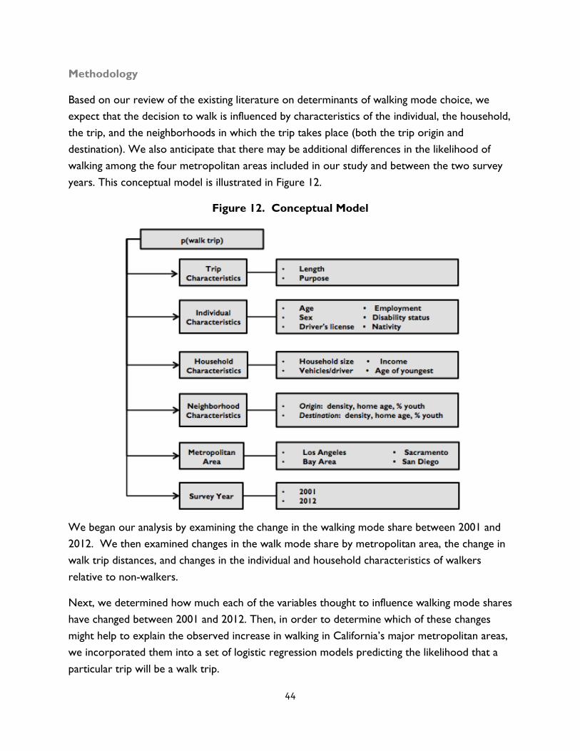
44
Methodology
Based on our review of the existing literature on determinants of walking mode choice, we
expect that the decision to walk is influenced by characteristics of the individual, the household,
the trip, and the neighborhoods in which the trip takes place (both the trip origin and
destination). We also anticipate that there may be additional differences in the likelihood of
walking among the four metropolitan areas included in our study and between the two survey
years. This conceptual model is illustrated in Figure 12.
Figure 12. Conceptual Model
We began our analysis by examining the change in the walking mode share between 2001 and
2012. We then examined changes in the walk mode share by metropolitan area, the change in
walk trip distances, and changes in the individual and household characteristics of walkers
relative to non-walkers.
Next, we determined how much each of the variables thought to influence walking mode shares
have changed between 2001 and 2012. Then, in order to determine which of these changes
might help to explain the observed increase in walking in California’s major metropolitan areas,
we incorporated them into a set of logistic regression models predicting the likelihood that a
particular trip will be a walk trip.

45
Several prior studies of walking behavior predict mode shares at the person or neighborhood
level.11 Others researchers have modeled mode choice at the trip level, and have found that
trip-level characteristics such as trip length and purpose have important effects on mode
choice12 By specifying our model at the trip-level, we are able to include these trip-level
relationships in our analysis.
Person-level and neighborhood-level models typically analyze built-environment effects on
mode share by estimating relationships between shares of walk trips and the built-environment
characteristics of travelers’ residential locations. However, many trips have origins or
destinations that outside the traveler’s residential neighborhood. In fact, as shown in Table 8,
about twenty percent of all trips in 2012 and nearly 30 percent of trips in 2001 had both an
origin and a destination that was not the traveler’s home. By estimating a trip-level model, we
are able to control for the built-environmental characteristics of trip origins and destinations,
rather than only characteristics of the traveler’s residential location.
For block-group density, we considered a model specification that included housing density and
employment density as separate variables and another that combines the two into a single
activity density variable indicating the number of jobs and homes per square kilometer. In all
models, income and density variables were log-transformed, since the effect of these variables is
more likely to be associated with proportional change (e.g. a ten percent increase) than with
absolute change (e.g. 100 additional homes or jobs per square km, or $6,000 of additional
income).
Since we excluded loop trips from the dataset, all trips have a distinct origin and destination.
However, since many trips take place within a neighborhood, or between similar
neighborhoods, the characteristics of trip origins and destinations are somewhat correlated,
especially for walk trips, as Table 6 shows. Nevertheless, the correlation is not strong enough
to preclude keeping both sets of neighborhood variables in the model if doing so provides the
best model fit.
Table 6. Correlations between trip origin and destination characteristics All trips Walk trips
Housing density 0.461 0.666
Employment density 0.340 0.754
Activity density 0.380 0.785
Housing age 0.428 0.672
Percent youth 0.228 0.713
11
See for example, Forsyth et al. (2009), Joh et al. (2015), Rodrıguez & Joo (2004), Weinberger & Sweet (2012). 12See, for example, Cervero & Duncan (2003), Kockleman (1997) and Manaugh & El-Geneidy (2013).

46
Table 7 compares the fit of six different sets of variables characterizing neighborhood densities.
Of these, the best-fitting model, as indicated by the lowest Akaike Information Criterion (AIC)
score is one that that combines housing and employment density into a single activity density
variable and includes information about both trip origins and destinations. Using this
neighborhood specification and the other variables listed from the conceptual model in Figure
12, we ran three logistic regression models: one including all observations from both years, a
second including only data from 2001, and a third including only data from 2012.
Table 7. Akaike Information Criterion (AIC) scores comparing model fit by
neighborhood variables
AIC score
Housing and employment
density combined into a single
activity density variable
Housing and employment density
as separate variables
Origins only 31,854 32,000
Destinations only 31,877 32,028
Origins and destinations 31,720 31,878
By comparing coefficient estimates between the 2001 and 2012 models, we identified variables
whose effect on walking mode choice varied by year. Based on these differences, we estimated
a fourth model in which we include data from both years, with interaction terms to determine
the change in effect size for those variables between 2001 and 2012.
Descriptive analysis
Figure 13 shows how mode shares have changed within the study area between 2001 and 2012.
The greatest change was a reduction in the share of trips by single-occupancy vehicle from 58
percent in 2001 to 47 percent in 2012. This difference is offset by an increase in multi-
occupancy vehicle trips from 33 to 41 percent (a 24 percent increase) and an increase in
walking trips from five to nine percent (an 80 percent increase).
Figure 13. Changes in mode shares within the study area, 2001-2012
58%
33%
5% 3% 1% 0%
47%41%
9%1% 1% 1%
0%10%20%30%40%50%60%70%
Sh
are
of
Tri
ps 2001
2012

47
As Figure 14 shows, the increase in walking mode share varied by metropolitan area. The most
modest gains were observed in the Los Angeles area, where the walking mode share increased
by about fifty percent. The Bay Area, which began with the highest walking mode share, saw an
increase of about 75 percent. Walking mode shares in both years were the lowest in the
Sacramento and San Diego areas. However, these areas saw the most dramatic increase in
walking; in both areas, the walking mode share increased about three-fold.
Figure 14. Increases in walking mode share by metropolitan area, 2001-2012
With the increases in walking mode share, we also observe changes in walk trip characteristics.
As shown in Figure 15, trip distance decreased for all modes between 2001 and 2012. The
average length of a walk trip declined from just under a mile in 2001 to half a mile in 2012. This
may indicate that short walk trips have become more common, or that the survey instrument
has improved to capture more short trips that had gone unreported in previous years.
8%6%
2% 2%
14%
9%
6%
7%
0%
2%
4%
6%
8%
10%
12%
14%
16%
Bay Area Los Angeles Sacramento San Diego
Walk
ing m
od
e s
hare
2001
2012
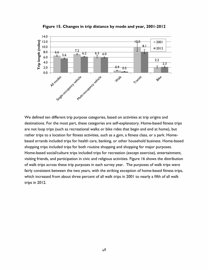
48
Figure 15. Changes in trip distance by mode and year, 2001-2012
We defined ten different trip purpose categories, based on activities at trip origins and
destinations. For the most part, these categories are self-explanatory. Home-based fitness trips
are not loop trips (such as recreational walks or bike rides that begin and end at home), but
rather trips to a location for fitness activities, such as a gym, a fitness class, or a park. Home-
based errands included trips for health care, banking, or other household business. Home-based
shopping trips included trips for both routine shopping and shopping for major purposes.
Home-based social/culture trips included trips for recreation (except exercise), entertainment,
visiting friends, and participation in civic and religious activities. Figure 16 shows the distribution
of walk trips across these trip purposes in each survey year. The purposes of walk trips were
fairly consistent between the two years, with the striking exception of home-based fitness trips,
which increased from about three percent of all walk trips in 2001 to nearly a fifth of all walk
trips in 2012.
6.67.2
6.3
0.9
10.0
2.2
5.66.2 6.0
0.5
8.1
2.3
0.0
2.0
4.0
6.0
8.0
10.0
12.0
14.0T
rip
len
gth
(m
iles) 2001
2012

49
Figure 16. Distribution of walk trips among trip purposes, 2001-2012
One explanation for the increase in walking may lie in reduced rates of driver’s licensure. As
Figure 17 shows, the share of the population without a driver’s increased from six percent 2001
to 11 percent in 2012. This increase was especially pronounced among those who made at least
one walking trip on the survey day (“walkers”).
Figure 17. Changes driver's license status among walkers and non-walkers, 2001-
2012
As shown in Figure 18, there were also large changes in employment status between 2001 and
2012, particularly in terms of the share of the population who were not in the workforce
(meaning they were neither employed nor looking for work. As with driver’s license status, this
difference was more pronounced for walkers than for non-walkers.
9%
14%
20%
25%
10% 10%
3% 3%3%
3%5%
10%
18% 20%16%
7%4%
18%
1% 1%
0%
5%
10%
15%
20%
25%
30%
35%P
erc
en
t o
f w
alk
tri
ps
2001
2012
6%
16%
5%
11%
24%
9%
0%
5%
10%
15%
20%
25%
30%
Everyone Walkers Non-walkers
Perc
en
t w
ith
ou
t a d
river'
s
licen
se
2001
2012

50
Figure 18. Changes in employment status among walkers and non-walkers, 2001-
2012
Figure 19 illustrates how household vehicle availability declined between 2001 and 2012. The
average number of household vehicles per driver declined in the households of both walkers
and non-walkers. In walker’s households, vehicle availability had declined to less than one
vehicle per licensed driver in 2012.
Figure 19. Changes in vehicle availability among walkers and non-walkers, 2001-
2012
Table 8 shows other observed changes between 2001 and 2012, based on a combination of
survey data and census data. Of particular interest for this study is the increase in the share of
71%63% 64%
55%72% 64%
20%32%
23%39%
20%31%
0%
20%
40%
60%
80%
100%
120%
Perc
en
t o
f sa
mp
le p
op
ula
tio
n
Not a worker
Unemployed
Employed
1.2
1.0
1.3
0.9
0.8
1.0
0.0
0.2
0.4
0.6
0.8
1.0
1.2
1.4
Everyone Walkers Non-walkers
Avera
ge p
ers
on
's h
ou
seh
old
veh
icle
s p
er
dri
ver
2001
2012
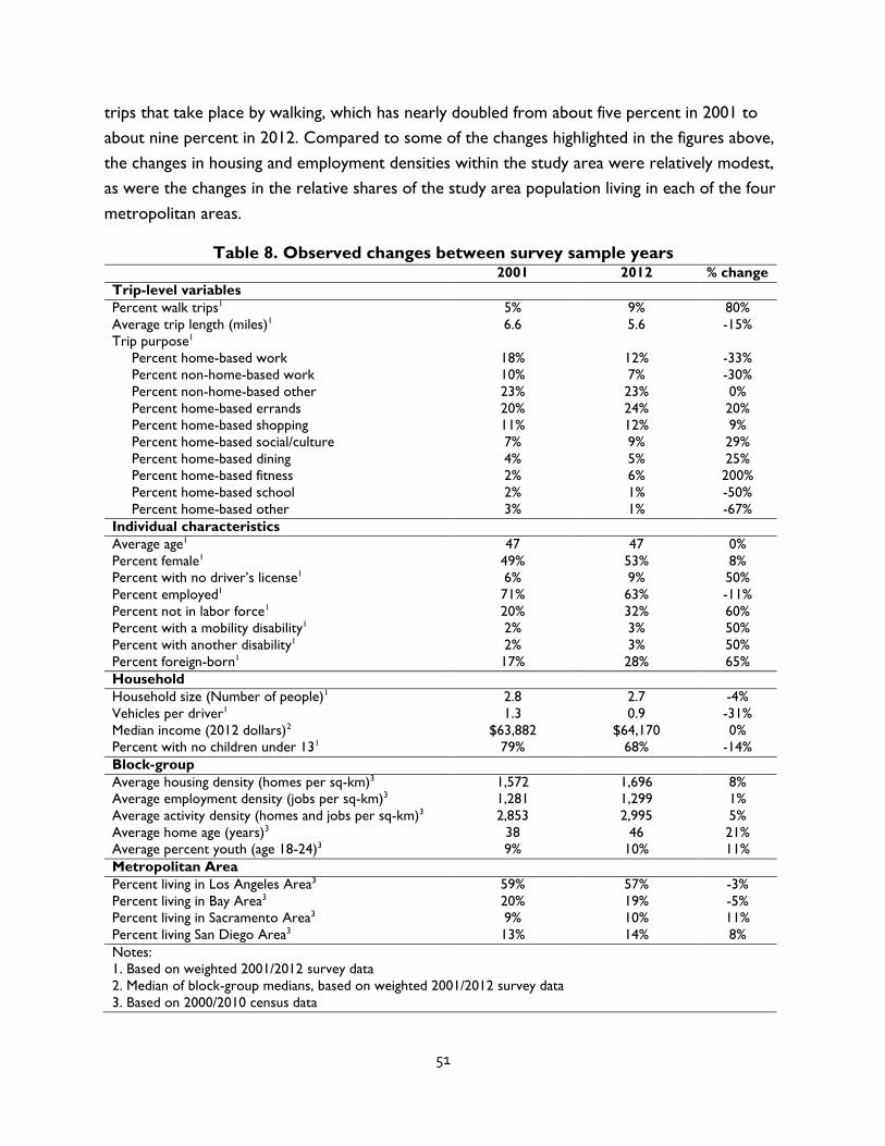
51
trips that take place by walking, which has nearly doubled from about five percent in 2001 to
about nine percent in 2012. Compared to some of the changes highlighted in the figures above,
the changes in housing and employment densities within the study area were relatively modest,
as were the changes in the relative shares of the study area population living in each of the four
metropolitan areas.
Table 8. Observed changes between survey sample years 2001 2012 % change
Trip-level variables
Percent walk trips1 5% 9% 80%
Average trip length (miles)1 6.6 5.6 -15%
Trip purpose1
Percent home-based work 18% 12% -33%
Percent non-home-based work 10% 7% -30%
Percent non-home-based other 23% 23% 0%
Percent home-based errands 20% 24% 20%
Percent home-based shopping 11% 12% 9%
Percent home-based social/culture 7% 9% 29%
Percent home-based dining 4% 5% 25%
Percent home-based fitness 2% 6% 200%
Percent home-based school 2% 1% -50%
Percent home-based other 3% 1% -67%
Individual characteristics
Average age1 47 47 0%
Percent female1 49% 53% 8%
Percent with no driver’s license1 6% 9% 50%
Percent employed1 71% 63% -11%
Percent not in labor force1 20% 32% 60%
Percent with a mobility disability1 2% 3% 50%
Percent with another disability1 2% 3% 50%
Percent foreign-born1 17% 28% 65%
Household
Household size (Number of people)1 2.8 2.7 -4%
Vehicles per driver1 1.3 0.9 -31%
Median income (2012 dollars)2 $63,882 $64,170 0%
Percent with no children under 131 79% 68% -14%
Block-group
Average housing density (homes per sq-km)3 1,572 1,696 8%
Average employment density (jobs per sq-km)3 1,281 1,299 1%
Average activity density (homes and jobs per sq-km)3 2,853 2,995 5%
Average home age (years)3 38 46 21%
Average percent youth (age 18-24)3 9% 10% 11%
Metropolitan Area
Percent living in Los Angeles Area3 59% 57% -3%
Percent living in Bay Area3 20% 19% -5%
Percent living in Sacramento Area3 9% 10% 11%
Percent living San Diego Area3 13% 14% 8%
Notes:
1. Based on weighted 2001/2012 survey data
2. Median of block-group medians, based on weighted 2001/2012 survey data
3. Based on 2000/2010 census data
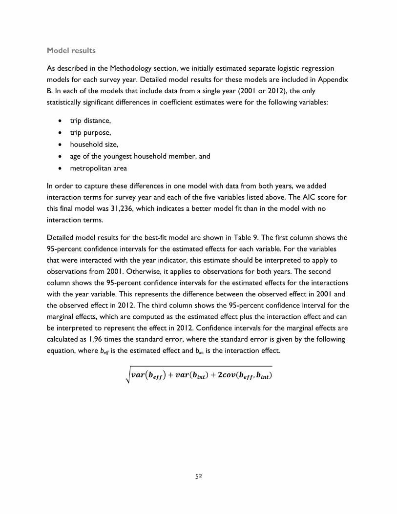
52
Model results
As described in the Methodology section, we initially estimated separate logistic regression
models for each survey year. Detailed model results for these models are included in Appendix
B. In each of the models that include data from a single year (2001 or 2012), the only
statistically significant differences in coefficient estimates were for the following variables:
trip distance,
trip purpose,
household size,
age of the youngest household member, and
metropolitan area
In order to capture these differences in one model with data from both years, we added
interaction terms for survey year and each of the five variables listed above. The AIC score for
this final model was 31,236, which indicates a better model fit than in the model with no
interaction terms.
Detailed model results for the best-fit model are shown in Table 9. The first column shows the
95-percent confidence intervals for the estimated effects for each variable. For the variables
that were interacted with the year indicator, this estimate should be interpreted to apply to
observations from 2001. Otherwise, it applies to observations for both years. The second
column shows the 95-percent confidence intervals for the estimated effects for the interactions
with the year variable. This represents the difference between the observed effect in 2001 and
the observed effect in 2012. The third column shows the 95-percent confidence interval for the
marginal effects, which are computed as the estimated effect plus the interaction effect and can
be interpreted to represent the effect in 2012. Confidence intervals for the marginal effects are
calculated as 1.96 times the standard error, where the standard error is given by the following
equation, where beff is the estimated effect and bint is the interaction effect.
√𝒗𝒂𝒓(𝒃𝒆𝒇𝒇) + 𝒗𝒂𝒓(𝒃𝒊𝒏𝒕) + 𝟐𝒄𝒐𝒗(𝒃𝒆𝒇𝒇, 𝒃𝒊𝒏𝒕)
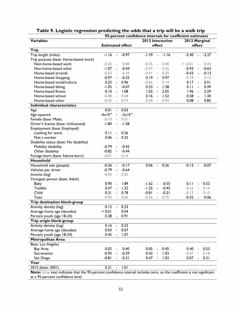
53
Table 9. Logistic regression predicting the odds that a trip will be a walk trip 95-percent confidence intervals for coefficient estimates
Variables
Estimated effect
2012 Interaction
effect
2012 Marginal
effect
Trip
Trip length (miles) -1.16 - -0.97 -1.39 - -1.16 -2.40 - -2.27
Trip purpose (base: Home-based work)
Non-home-based work -0.20 - 0.48 -0.35 - 0.40 > -0.01 - 0.33
Non-home-based other -1.07 - -0.44 -0.37 - 0.32 -0.93 - -0.63
Home-based errands -0.53 - 0.10 -0.41 - 0.29 -0.43 - -0.13
Home-based shopping -0.97 - -0.25 0.19 - 0.97 -0.19 - 0.12
Home-based social/culture 0.23 - 0.96 -0.66 - 0.14 0.17 - 0.51
Home-based dining -1.05 - -0.07 0.33 - 1.38 0.11 - 0.49
Home-based fitness 0.10 - 1.08 1.02 - 2.05 1.96 - 2.29
Home-based school -0.48 - 0.68 0.16 - 1.52 0.58 - 1.30
Home-based other -0.35 - 0.74 -0.39 - 0.94 0.08 - 0.85
Individual characteristics
Age 0.01 - 0.03
Age squared -4x10⁻⁴ - -2x10⁻⁴
Female (base: Male) -0.10 - 0.01
Driver’s license (base: Unlicensed) -1.80 - -1.58
Employment (base: Employed)
Looking for work 0.11 - 0.26
Not a worker 0.06 - 0.32
Disability status (base: No disability)
Mobility disability -0.79 - -0.42
Other disability -0.82 - -0.44
Foreign-born (base: Native-born) -0.01 - 0.14
Household
Household size (people) -0.36 - -0.17 0.06 - 0.26 -0.13 - -0.07
Vehicles per driver -0.79 - -0.64
Income (log) -0.05 - 0.02
Youngest person (base: Adult)
Baby 0.90 - 1.89 -1.62 - -0.55 0.11 - 0.52
Toddler 0.47 - 1.22 -1.25 - -0.45 -0.16 - 0.14
Child 0.21 - 0.78 -0.81 - -0.21 -0.12 - 0.10
Teen -0.92 - 0.06 -0.26 - 0.75 -0.32 - -0.06
Trip destination block-group
Activity density (log) 0.15 - 0.23
Average home age (decades) < 0.01 - 0.04
Percent youth (age 18-24) 0.28 - 0.91
Trip origin block-group
Activity density (log) 0.16 - 0.23
Average home age (decades) 0.03 - 0.07
Percent youth (age 18-24) 0.45 - 1.07
Metropolitan Area
Base: Los Angeles
Bay Area 0.02 - 0.40 0.05 - 0.45 0.40 - 0.53
Sacramento -0.95 - -0.39 0.42 - 1.03 -0.07 - 0.18
San Diego -0.81 - -0.31 0.47 - 1.03 0.07 - 0.31
Year
2012 (base: 2001) 0.21 - 1.01
Note: Gray text indicates that the 95-percent confidence interval includes zero, so the coefficient is not significant
at a 95-percent confidence level.

54
All of the individual characteristics and block-group characteristics had the same relationship
with the likelihood of walking in both survey years, as did two household characteristics:
household income and the number of household vehicles per driver.
As shown Table 9 and illustrated in Figure 20, the traveler’s age has a modest, but statistically
significant effect on the likelihood that a trip will be made by walking. Holding other variables
constant, for a person with a ten-percent probability of making a walk trip, the probability of
walking increases slightly until peaking at 13 percent in the traveler’s mid-thirties, then steadily
decreases to less than three percent by the traveler’s mid-eighties.
Figure 20. Effect of age on the probability of walking
Neither sex nor nativity has a statistically significant effect on the odds that a trip will be a walk
trip. As shown in Figure 21, driver’s licensure, employment, disability, and household vehicle
availability all have statistically significant relationships with the odds that a trip will be a walk
trip.
0%
5%
10%
15%
20%
25%
30%
35%
40%
45%
50%
18 22 26 30 34 38 42 46 50 54 58 62 66 70 74 78 82
Pro
bab
ilit
y o
f w
alk
ing, fo
r a p
ers
on
wh
o w
ou
ld h
ave h
ad
a
10%
pro
bab
ilit
y o
f w
alk
ing if
they w
ere
18 y
ears
old
Age
95-percent
confidence interval

55
For people who are not employed, either because they are not in the work force or because
they have not found employment, the odds of a given trip being a walk trip are about twenty
percent higher than for people who are employed.
Disability (whether mobility or other disability) reduces the odds that a trip will take place by
walking, and the magnitude of this effect is about the same as that of adding an additional
household vehicle per driver. Having a driver’s license likewise reduces the odds of walking, and
the magnitude of this effect is about twice that of having a disability or adding an additional
vehicle per driver.
Figure 21. Effects of licensure, employment, disability, and vehicle availability on
the odds of walking
Figure 22 illustrates the effects of three block-group characteristics at the trip origin and
destination on the odds that a trip will be a walk trip. For the most part, the effects are modest.
Doubling the activity density at either the trip origin or trip destination is associated with an
increase of just under twenty percent in the odds of walking. This would be about the same as
the effect of increasing the average block-group housing age by over 40 years or increasing the
share of young people by about 25 percentage points.
-200% -150% -100% -50% 0% 50% 100% 150% 200%
Not in work force (compared to employed)
Unemployed (compared to employed)
Percent change in the odds that a trip will be a walk trip
Licensed driver (compared to unlicensed)
Mobility disability (compared to no disability)
Other disability (compared to no disability)
One additional household vehicle per driver
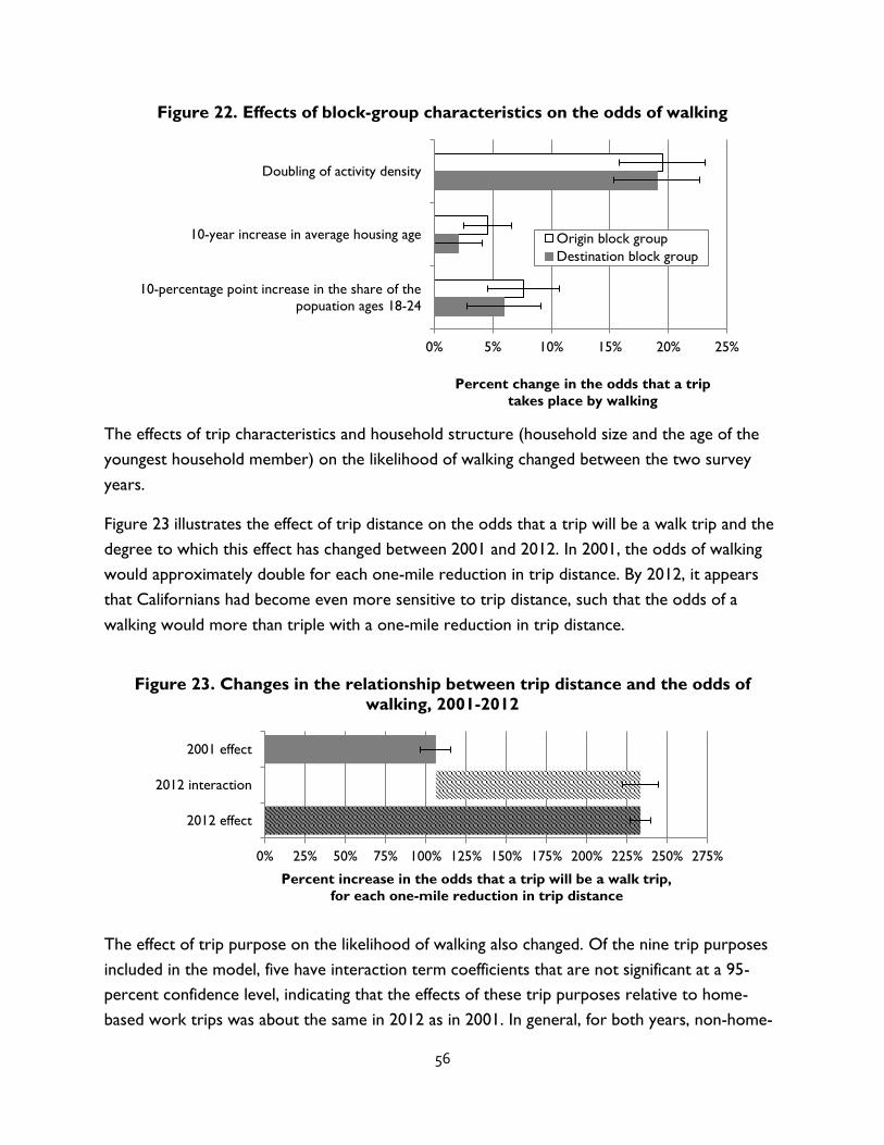
56
Figure 22. Effects of block-group characteristics on the odds of walking
The effects of trip characteristics and household structure (household size and the age of the
youngest household member) on the likelihood of walking changed between the two survey
years.
Figure 23 illustrates the effect of trip distance on the odds that a trip will be a walk trip and the
degree to which this effect has changed between 2001 and 2012. In 2001, the odds of walking
would approximately double for each one-mile reduction in trip distance. By 2012, it appears
that Californians had become even more sensitive to trip distance, such that the odds of a
walking would more than triple with a one-mile reduction in trip distance.
Figure 23. Changes in the relationship between trip distance and the odds of
walking, 2001-2012
The effect of trip purpose on the likelihood of walking also changed. Of the nine trip purposes
included in the model, five have interaction term coefficients that are not significant at a 95-
percent confidence level, indicating that the effects of these trip purposes relative to home-
based work trips was about the same in 2012 as in 2001. In general, for both years, non-home-
0% 5% 10% 15% 20% 25%
Doubling of activity density
10-year increase in average housing age
10-percentage point increase in the share of the
popuation ages 18-24
Percent change in the odds that a trip
takes place by walking
Origin block group
Destination block group
0% 25% 50% 75% 100% 125% 150% 175% 200% 225% 250% 275%
2001 effect
2012 interaction
2012 effect
Percent increase in the odds that a trip will be a walk trip,
for each one-mile reduction in trip distance

57
based work trips, home-based errand trips, and home-based other trips were as likely to be
walk trips as home-based work trips were. Non-home-based other trips were less likely to be
walk trips than home-based work trips were, and home-based social/cultural trips were more
likely.
Figure 24 illustrates the changes in the effect of trip purpose on walking between 2001 and
2012 for the trip purposes where these changes were significant. In 2001, home-based
shopping trips were less likely than home-based work trips to be walk trips. By 2012, this effect
seems to have disappeared, so that home-based shopping trips are about as likely as home-
based work trips are to be walk trips.
For home-based dining trips, the change in the effect between 2001 and 2012 was even more
dramatic: enough to change the direction of the effect relative to home-based work trips.
While home-based dining trips were less likely than work trips to be walk trips in 2001, they
were more likely than home-based work trips to be walk trips in 2012.
In 2001, the odds of a trip being a walk trip were just over fifty percent higher for home-based
fitness trips than for home-based work trip. By 2012, this already large effect had grown so that
the odds of walking for a home-based fitness trip were more than triple those for a home-
based work trip.
Finally, in 2001, home-based school trips were no more likely to be walk trips than home-based
work trips were. However, by 2012, the odds of walking for a home-based school trip were
almost double those for a home-based work trip.

58
Figure 24. Effects of trip purpose on the odds of walking
Figure 25. Effect of household size on the odds of walking
As Figure 25 shows, larger households are associated with increased odds that a trip by a
household member will be a walk trip, although the magnitude of the effect is much smaller in
2012 than in 2001. In addition to the number of household members, the ages of household
members also relates to the likelihood that a trip will take place by walking. Figure 26 illustrates
the effect of household children on the odds that a trip will be a walk trip. In general, children
make it more likely that a trip will be a walk trip. In 2001, the greatest effect is observed for the
presence of a baby, and the second-greatest effect is for the presence of a toddler. This pattern
-150% -100% -50% 0% 50% 100% 150% 200% 250% 300%
Percent change in the odds that a trip will be a walk trip,
relative to a home-based work trip
2001 effect
2012 Interaction effect
2012 marginal effect
Home-based
shopping
Home-based
fitness
Home-based
school
Home-based
dining
0% 5% 10% 15% 20% 25% 30% 35% 40%
2001 effect
2012 interaction
2012 effect
Percent increase in the odds that a trip will be a walk trip,
for each one-person reduction in household size

59
continues in 2012, but all effects are diminished so that only the effect of the presence of a baby
is associated with a significant increase in the odds that a trip will be a walk trip. The presence
of teenagers in a household does not have a significant effect on the odds of walking on a given
trip in 2001, but by 2012, household teenagers were associated with reduced odds of walking.
Figure 26. Effect of the presence of children on the odds of walking
Figure 27 illustrates the differences in the odds of walking among metropolitan areas and
between years. In 2001, a trip in the Bay Area was more likely to be a walk trip than a trip in
the Los Angeles area was, and this difference had more than doubled by 2012. In 2001, trips in
San Diego and Sacramento were both less likely than trips in Los Angeles to be walk trips. By
2012, this difference had disappeared in Sacramento and reversed itself in San Diego.
-100% -50% 0% 50% 100% 150% 200% 250%
Percent change in the odds that a trip will be a walk trip,
relative to one in a household with no children
2001 effect
2012 Interaction effect
2012 marginal effect
Youngest household
member is a baby
Youngest household
member is a toddler
Youngest household
member is child
Youngest household
member is a teen

60
Figure 27. Effects of metropolitan area on the odds of walking
Discussion
In general, trip characteristics (trip distance and trip purpose) have the greatest effects on the
odds of walking, and the magnitudes of these effects have increased between 2001 and 2012.
Individual and neighborhood characteristics have more modest effects on the odds of walking,
and these effects are consistent between the two survey years.
Table 10 identifies 18 different characteristics for which a change would be expected to
increase walking mode shares (by increasing the odds that any particular trip will be a walk
trip). For 12 of these 18 characteristics, the change that would have increased walking is the
change that was observed. In fact, for three characteristics—trip length, the share of home-
based fitness trips, and the share of the study population living in the Bay Area—not only did
change occur in a direction consistent with increased walking, but the influence of these factors
on walking also increased between 2001 and 2012, magnifying the effect of these changes. For
four of the 18 characteristics where a change could have contributed to increased walking, the
change that occurred was in the opposite direction to one consistent with more walking.
However, in all four cases, the effect of that quantity on walking had either been eliminated or
reversed by 2012.
Taken together, these results suggest that several changes occurred within California
metropolitan areas between 2001 and 2012 that contributed to the observed increases in
walking. Further, we found no counterbalancing changes appear to have mitigated the effects of
-120% -100% -80% -60% -40% -20% 0% 20% 40% 60% 80%
Percent change in the odds that a trip will be a walk trip,
relative to a trip in the Los Angeles metropolitan area
2001 effect
2012 Interaction effect
2012 marginal effect
Bay Area
Sacramento
San Diego
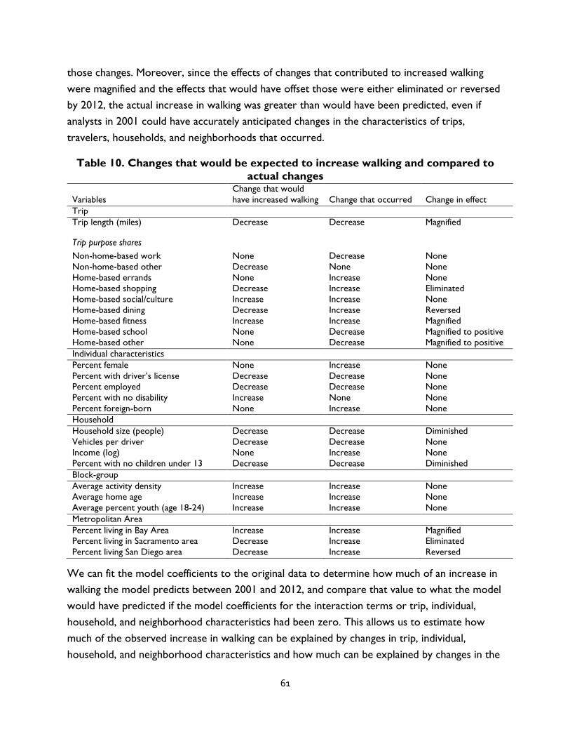
61
those changes. Moreover, since the effects of changes that contributed to increased walking
were magnified and the effects that would have offset those were either eliminated or reversed
by 2012, the actual increase in walking was greater than would have been predicted, even if
analysts in 2001 could have accurately anticipated changes in the characteristics of trips,
travelers, households, and neighborhoods that occurred.
Table 10. Changes that would be expected to increase walking and compared to
actual changes
Variables
Change that would
have increased walking Change that occurred Change in effect
Trip
Trip length (miles) Decrease Decrease Magnified
Trip purpose shares
Non-home-based work None Decrease None
Non-home-based other Decrease None None
Home-based errands None Increase None
Home-based shopping Decrease Increase Eliminated
Home-based social/culture Increase Increase None
Home-based dining Decrease Increase Reversed
Home-based fitness Increase Increase Magnified
Home-based school None Decrease Magnified to positive
Home-based other None Decrease Magnified to positive
Individual characteristics
Percent female None Increase None
Percent with driver’s license Decrease Decrease None
Percent employed Decrease Decrease None
Percent with no disability Increase None None
Percent foreign-born None Increase None
Household
Household size (people) Decrease Decrease Diminished
Vehicles per driver Decrease Decrease None
Income (log) None Increase None
Percent with no children under 13 Decrease Decrease Diminished
Block-group
Average activity density Increase Increase None
Average home age Increase Increase None
Average percent youth (age 18-24) Increase Increase None
Metropolitan Area
Percent living in Bay Area Increase Increase Magnified
Percent living in Sacramento area Decrease Increase Eliminated
Percent living San Diego area Decrease Increase Reversed
We can fit the model coefficients to the original data to determine how much of an increase in
walking the model predicts between 2001 and 2012, and compare that value to what the model
would have predicted if the model coefficients for the interaction terms or trip, individual,
household, and neighborhood characteristics had been zero. This allows us to estimate how
much of the observed increase in walking can be explained by changes in trip, individual,
household, and neighborhood characteristics and how much can be explained by changes in the

62
relationship between these characteristics and the odds of walking. These proportions are
illustrated in Figure 28. As shown, about 40 percent of the observed increase in walking can be
explained by changes in the relationships between walking and each trip, individual, household,
and neighborhood characteristic (for example, increased sensitivity to trip distance). The
remaining 60 percent of the observed increase can be explained by changes the characteristics
themselves (for example, reduced trip lengths, smaller household sizes, and higher densities), as
well as changes in the relative shares of population living in each MSA (for example, the
increased share of the study area population living in the Bay Area).
Figure 28. Increase in walking attributable to changes in trip, individual, household,
and neighborhood characteristics
Differences in trip characteristics (trip distance and trip purpose) explain about a quarter of the
observed increase in walking. Differences among the four metropolitan areas that are not
otherwise accounted for in the model contribute another 13 percent of the observed increase.
Changes in neighborhood characteristics (density, age of housing stock, and percent youth)
account for 10 percent of the increase.
Change in trip
characteristics
25%
Changes in individual characteristics
7%
Changes in
household
characteristics
4%
Changes in
neighborhood
characteristics
10%Changes in relative
MSA populations
13%
Changes in effects
of trip, household,
and neighborhood
characteristics
41%

63
Conclusion
The findings of this study suggest two important insights that should inform local planning for
pedestrians.
First, dramatic increases in walking are most likely to occur in connection with a confluence of
factors. While many of the factors associated with increased walking are beyond the control of
planners and policy makers, others may be influenced by planning and policy decisions. For
example, more walk trips are likely to result from land use plans that bring origins and
destinations closer together, especially for trip destinations that are already attractive for
walking, such as entertainment, culture, fitness, and recreation destinations, including parks and
open space. Likewise, improving the proximity of family- and child-oriented amenities, such as
high-quality schools and childcare facilities can increase opportunities for walking by members
of households with young children, who are already more inclined to walk than their peers.
These types of changes that could serve to reduce trip distances could become increasingly
effective in light of our finding that the decision to walk has become more sensitive to trip
distance since 2001.
Second, the significant changes in the effects of our explanatory variables over time highlights
the importance of frequent updates and recalibration of planning models that use these
relationships to predict future travel demand, since these relationships are not constant over
time. The danger of under-predicting walking mode shares is two-fold: first, it may lead planners
and policy makers to inadequately invest in walking amenities that can make walking safer and
more pleasant for the growing number of travelers who use this transportation mode. Second,
failure to accurately predict walking travel demand may lead to overinvestment in far more
expensive transportation infrastructure for motorized transportation modes.
There is a need for further research that examines changes in walking behavior over time. One
barrier to conducting such studies is a paucity of detailed time-series data about the
characteristics of built environment that are believed to influence the decisions to walk, such as
the presence and quality of pedestrian amenities. A second barrier is the lack of frequent travel
surveys that are designed to capture short, non-commute trips; these trips are the most likely
to walk trips, but have not been the focus of traditional travel surveys that have emphasized
regional travel. As data on travel and the built environment continue to improve in detail,
consistency over time, and collection frequency, researchers will be in position to greatly
improve the current understanding of the determinants of the decision to walk and factor that
are most likely to cause changes in walking behavior.

64
References
Badland, H., & Schofield, G. (2005). Transport, Urban Design And Physical Activity: An
Evidence-Based Update. Transportation Research Part D, 10, 177–196.
Bassett Jr, D. R., Pucher, J., Buehler, R., Thompson, D. L., & Crouter, S. E. (2008). Walking,
Cycling, and Obesity Rates in Europe, North America, and Australia. J Phys Act Health, 5(6),
795–814.
Boarnet, M. G., Day, K., Anderson, C., McMillan, T., & Alfonzo, M. (2005). California’s Safe
Routes To School Program: Impacts On Walking, Bicycling, And Pedestrian Safety. Journal of the
American Planning Association, 71(3), 301–317.
Brown, B. B., Werner, C. M., Tribby, C. P., Miller, H. J., & Smith, K. R. (2015). Transit Use,
Physical Activity, and Body Mass Index Changes: Objective Measures Associated With
Complete Street Light-Rail Construction. American Journal of Public Health, 105(7), 1468–1474.
http://doi.org/10.2105/AJPH.2015.302561
Cervero, R., & Duncan, M. (2003). Walking, Bicycling, and Urban Landscapes: Evidence From
the San Francisco Bay Area. American Journal of Public Health, 93(9), 1478–1483.
Clifton, K. J., & Krizek, K. J. (2004). The Utility of the NHTS in Understanding Bicycle and
Pedestrian Travel (pp. 1–2). Presented at the National Household Travel Survey Conference:
understanding our nation’s travel.
Ewing, R., & Cervero, R. (2010). Travel and the Built Environment. Journal of the American
Planning Association, 76(3), 265–294.
Forsyth, A., Michael Oakes, J., Lee, B., & Schmitz, K. H. (2009). The Built Environment, Walking,
and Physical Activity: Is the Environment More Important to Some People than Others?
Transportation Research Part D: Transport and Environment, 14(1), 42–49.
http://doi.org/10.1016/j.trd.2008.10.003
Freeland, A. L., Banerjee, S. N., Dannenberg, A. L., & Wendel, A. M. (2013). Walking Associated
with Public Transit: Moving Toward Increased Physical Activity in the United States. American
Journal of Public Health, 103(3), 536–542.
Goodman, A., Sahlqvist, S., & Ogilvie, D. (2014). New Walking and Cycling Routes and
Increased Physical Activity: One-And 2-Year Findings from the UK Iconnect Study. American
Journal of Public Health, 104(9), e38–e46.

65
Gordon-Larsen, P., Hou, N., Sidney, S., Sternfeld, B., Lewis, C. E., Jacobs, D. R., & Popkin, B. M.
(2009). Fifteen-Year Longitudinal Trends in Walking Patterns and Their Impact on Weight
Change. The American Journal of Clinical Nutrition, 89(1), 19–26.
Ham, S. A., Macera, C. A., & Lindley, C. (2005). Trends in Walking for Transportation in the
United States, 1995 and 2001. Preventing Chronic Disease, 2(4), A14.
Joh, K., Chakrabarti, S., Boarnet, M. G., & Woo, A. (2015). The Walking Renaissance: A
Longitudinal Analysis of Walking Travel in the Greater Los Angeles Area, USA. Sustainability,
7(7), 8985–9011.
Kockelman, K. (1997). Travel Behavior as Function of Accessibility, Land Use Mixing, and Land
Use Balance: Evidence from San Francisco Bay Area. Transportation Research Record: Journal of the
Transportation Research Board, 1607, 116–125. http://doi.org/10.3141/1607-16
MacDonald, J. M., Stokes, R. J., Cohen, D. A., Kofner, A., & Ridgeway, G. K. (2010). The Effect
of Light Rail Transit on Body Mass Index and Physical Activity. American Journal of Preventive
Medicine, 39(2), 105–112.
Manaugh, K., & El-Geneidy, A. (2011). Validating Walkability Indices: How Do Different
Households Respond to the Walkability of their Neighborhood? Transportation Research Part D:
Transport and Environment, 16(4), 309–315.
McCormack, G. R., & Shiell, A. (2011). In Search Of Causality: A Systematic Review of the
Relationship Between the Built Environment and Physical Activity Among Adults. International
Journal of Behavioral Nutrition and Physical Activity, 8(1), 125. http://doi.org/10.1186/1479-5868-8-
125
McKenzie, B. (2014). Modes Less Traveled—Bicycling and Walking to Work in the United
States: 2008–2012. US Census Bureau, New York.
Ogilvie, D., Foster, C. E., Rothnie, H., Cavill, N., Hamilton, V., Fitzsimons, C. F., Mutrie, N.,
Scottish Physical Activity Research Collaboration. (2007). Interventions to promote walking:
systematic review. Bmj.
Pucher, J., Buehler, R., Merom, D., & Bauman, A. (2011). Walking and Cycling in the United
States, 2001–2009: Evidence from the National Household Travel Surveys. American Journal of
Public Health, 101(S1), S310–S317.

66
Rodrı ́guez, D. A., & Joo, J. (2004). The Relationship between Non-Motorized Mode Choice and
the Local Physical Environment. Transportation Research Part D: Transport and Environment, 9(2),
151–173.
Saelens, B. E., & Handy, S. L. (2008). Built Environment Correlates of Walking: A Review.
Medicine and Science in Sports and Exercise, 40(7 Suppl), S550–S566.
Santos, A., McGuckin, H., Nakamoto, Gray, D., & Liss, S. (2011). Summary of Travel Trends: 2009
National Household Travel Survey (Trends in Travel Behavior, 1969-2009 No. FHWA-PL-11-022).
Washington, D.C.: US Department of Transportation.
Simpson, M. E., Serdula, M., Galuska, D. A., Gillespie, C., Donehoo, R., Macera, C., & Mack, K.
(2003). Walking Trends among US Adults: The Behavioral Risk Factor Surveillance System,
1987–2000. American Journal of Preventive Medicine, 25(2), 95–100.
Stopher, P. R., & Greaves, S. P. (2007). Household Travel Surveys: Where Are We Going?
Transportation Research Part A: Policy and Practice, 41(5), 367–381.
Talen, E. (2002). Pedestrian Access as a Measure of Urban Quality. Planning Practice and
Research, 17(3), 257–278.
Tudor-Locke, C., Van Der Ploeg, H. P., Bowles, H. R., Bittman, M., Fisher, K., Merom, D.,
Gershuny, J., Bauman, A., Egerton, M. (2007). Walking Behaviours from the 1965–2003
American Heritage Time Use Study (AHTUS). International Journal of Behavioral Nutrition and
Physical Activity, 4(1), 45.
Weinberger, R., & Sweet, M. (2012). Integrating Walkability into Planning Practice.
Transportation Research Record: Journal of the Transportation Research Board, (2322), 20–30.

67
IV. Change, change, change: The relationship between changes in neighborhood
characteristics and changes in walking
Introduction
Previous studies (Ham et al., 2005; Joh et al., 2015; Pucher et al., 2011; Santos et al., 2011;
Simpson et al., 2003; Tudor-Locke et al., 2007) as well as our analysis in Chapter III show that
rates of walking have increased over time. Yet only one of these studies analyzes whether
changes in neighborhood characteristics might contribute to observed changes in walking mode
choice within specific neighborhoods. This study seeks to address this gap in the literature by
examining the relationship between changes in walking mode choice and changes in other
neighborhood characteristics within California neighborhoods. To assemble a large enough
sample of census tracts, we draw on data from the 2001 and 2012 California Household Travel
Survey from throughout the state. We determine the change in walking mode choice in a
sample of over 1,300 California census tracts, which are home to 20 percent of the state’s
population, and which included enough trips to perform this analysis. We then use a Tobit
regression model to determine the degree to which these changes may be explained by changes
over time in the socioeconomic and built environment characteristics of these census tracts.
We find that changes in two census tract characteristics are associated with changes in walking
mode choice. First, walking and poverty rates are inversely related; a one percent reduction in
the poverty rate within a census tract is associated with a 0.4 percent increase in walking mode
share. Second, a one percent increase in intersection density is associated with a 0.75 percent
increase in walking mode share. These findings suggest three types of policy efforts to increase
walking mode shares: (1) policies to reduce poverty, (2) policies to minimize the effects of
poverty on walking mode choice, and (3) development patterns characterized by high
intersection density and pedestrian route directness.
Determinants of changes in walking mode share
Data from a variety of sources show an increase in walking mode share over time in the U.S.
(See Appendix A for a summary of these studies.) The National Household Travel Survey
(NHTS), a national inventory of daily travel in the U.S., shows that the percentage of trips taken
on foot increased from 8.6 percent in 2001 to 10.4 percent in 2009 (Santos et al., 2011). There
was also a 28 percent increase in the number people accessing transit by walking from 2001 to
2009 (Freeland et al., 2013). Due to inconsistencies in collecting data on walk trips, it is difficult
to identify from previous national travel surveys the start of this upward trend (Clifton &
Krizek, 2004). Traditional travel surveys tend to undercount short trips, many of which are
taken on foot (Stopher & Greaves, 2007), and the NHTS only began specifically instructing

68
survey respondents to report walk trips in 2001 (Santos et al., 2011). However, there is some
evidence that walking mode shares in the United States have been increasing since as early as
1995. For example, in a study of short trips (one mile or less) Ham et al. (2005) find an increase
in walking mode share between 1995 and 2001.
Walking rates have increased according to data from other studies, a finding that validates the
trends from national travel surveys. For example, the Behavioral Risk Factor Surveillance
System (BRFSS) is sponsored by a number of federal agencies including the Centers for Disease
Control and Prevention, and is the nation's premier system of health-related telephone surveys.
Data from the BRFSS show an increase in the prevalence of leisure walking from 1987-2000
(Simpson et al., 2003). Similarly, data from the American Heritage Time Use Study find an
increase in the percentage of adults that walks for exercise from 2.9 percent in 1985 to 5.4
percent in 2003 (Tudor-Locke et al., 2007). The duration of time adults spent walking for
exercise also increased from 30 to 45 minutes per day.
Increases in walking are not been uniform across population groups. Low-income adults,
women, minorities, and working-age adults have experienced the largest increases in walking
(Freeland et al., 2013; Pucher et al., 2011; Simpson et al., 2003). In contrast, rates of walking
among seniors have lagged (Pucher et al., 2011). Data from the 2001 and 2009 NHTS show that
the elderly (65 years and older) reported a decline across two measures – the percentage that
walked per week (45 percent to 41 percent) and the percentage that took five or more walk
trips per week (from 31 percent to 30 percent) (Pucher et al., 2011). Increases in walking also
vary across cities. As might be expected, the percentage of workers that walk to work is
highest in large, dense cities such as Boston (15 percent), Washington, DC (12 percent) and
New York (10.3 percent) (McKenzie, 2014). However, among the largest 50 cities, only Atlanta,
Boston, Chicago, Cleveland, Omaha, Sacramento, San Jose, and Seattle experienced statistically
significant gains from 2000 to 2008-2012 in the percentage of people that walked to work
(McKenzie, 2014).
Amidst these promising trends, these data suggest a few areas of concern. First, despite
numerous planning efforts aimed at creating walkable, mixed-use communities, there has been a
substantial decline in the percentage of commuters that walk to work. The walk commute
share fell from 5.6 percent in 1980 to 2.8 percent in 2008-12 (McKenzie, 2014). This finding
may or may not be troublesome since commute trips comprise only 16 percent of all trips
(Santos et al., 2011). Second, perhaps more problematic is the fact that despite increases in
walking, even people who are walking still are not active enough to meet national public health
goals. Simpson et al. (2003) find no increase in the prevalence of people meeting the

69
recommendation for moderate physical activity for at least 30 minutes per day, five or more
days per week. Only 20 percent met this goal, a figure well below the 30 percent target.
All of these studies suggest that walking is becoming an increasingly important mode of
transportation, but in order to ensure that these promising trends continue, planners and policy
makers need a better understanding of the factors that explain the observed increases in
walking. There is a large and growing body of research on the determinants of walking, much of
it focused on the relationship between the built environment and walking behavior.13 For the
most part, these have been cross-sectional studies. While cross-sectional studies offer some
insight into the effects that changes in individual, household, and neighborhood characteristics
may have on changes in walking behavior, they are less relevant than longitudinal studies based
on observed changes over time.
Of the longitudinal studies on walking behavior that have been completed, most have been
limited in their geographic scope and have assessed the effects of specific interventions. Ogilvie
et al. (2007) review 19 randomized controlled trials and 29 non-randomized controlled studies
and find that:
Interventions tailored to people’s needs, targeted at the most sedentary or at
those most motivated to change, and delivered either at the level of the
individual (brief advice, supported use of pedometers, telecommunications) or
household (individualised marketing) or through groups, can encourage people
to walk more, although the sustainability, generalisability, and clinical benefits of
many of these approaches are uncertain (Ogilvie et al., 2007, p. 1).
The most successful of these interventions increased walking by up to 30-60 minutes a week on
average, at least in the short term. A few studies examine the relationship between
infrastructure investments and walking. These studies suggest that safety improvements and the
provision of high-quality, traffic-free walking routes increased walking; the largest effects were
among individuals without automobiles (Boarnet et al., 2005; Goodman et al., 2014).
Additionally, studies of household travel behavior before and after the opening of light rail
systems find associations between light rail use and physical activity through walking (Brown et
al., 2015; MacDonald et al., 2010).
A study by Joh et al. (2015) is unique; it is a longitudinal study of changes in walking behavior
over a relatively large geographic area—the Los Angeles combined statistical area (CSA)—
using geographic areas—46 regional statistical areas (RSAs)—as the unit of analysis. Rather than
evaluating the effects of a specific intervention, they use a fixed-effects model to determine
13
See Badland & Schofield (2005), Saelens & Handy (2008), Ewing & Cervero (2010), McCormack & Shiell (2011)
for reviews of this literature.
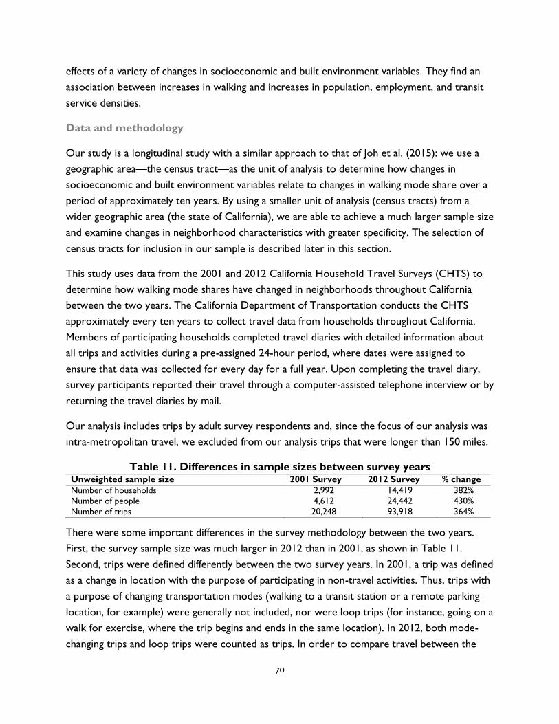
70
effects of a variety of changes in socioeconomic and built environment variables. They find an
association between increases in walking and increases in population, employment, and transit
service densities.
Data and methodology
Our study is a longitudinal study with a similar approach to that of Joh et al. (2015): we use a
geographic area—the census tract—as the unit of analysis to determine how changes in
socioeconomic and built environment variables relate to changes in walking mode share over a
period of approximately ten years. By using a smaller unit of analysis (census tracts) from a
wider geographic area (the state of California), we are able to achieve a much larger sample size
and examine changes in neighborhood characteristics with greater specificity. The selection of
census tracts for inclusion in our sample is described later in this section.
This study uses data from the 2001 and 2012 California Household Travel Surveys (CHTS) to
determine how walking mode shares have changed in neighborhoods throughout California
between the two years. The California Department of Transportation conducts the CHTS
approximately every ten years to collect travel data from households throughout California.
Members of participating households completed travel diaries with detailed information about
all trips and activities during a pre-assigned 24-hour period, where dates were assigned to
ensure that data was collected for every day for a full year. Upon completing the travel diary,
survey participants reported their travel through a computer-assisted telephone interview or by
returning the travel diaries by mail.
Our analysis includes trips by adult survey respondents and, since the focus of our analysis was
intra-metropolitan travel, we excluded from our analysis trips that were longer than 150 miles.
Table 11. Differences in sample sizes between survey years Unweighted sample size 2001 Survey 2012 Survey % change
Number of households 2,992 14,419 382%
Number of people 4,612 24,442 430%
Number of trips 20,248 93,918 364%
There were some important differences in the survey methodology between the two years.
First, the survey sample size was much larger in 2012 than in 2001, as shown in Table 11.
Second, trips were defined differently between the two survey years. In 2001, a trip was defined
as a change in location with the purpose of participating in non-travel activities. Thus, trips with
a purpose of changing transportation modes (walking to a transit station or a remote parking
location, for example) were generally not included, nor were loop trips (for instance, going on a
walk for exercise, where the trip begins and ends in the same location). In 2012, both mode-
changing trips and loop trips were counted as trips. In order to compare travel between the

71
two years, we removed all loop trips from the 2012 data set and linked all mode-changing trips
together to identify the trips’ ultimate origins and destinations. Walk trips were defined as trips
for which all segments took place by walking.
The confidential data from the CHTS includes the latitude and longitude coordinates for each
trip end. Using these coordinates, we geocoded each trip origin and assigned it to a census
tract. For each census tract, we calculated the walking mode share by determining the
proportion of trips originating in the tract that took place entirely by walking, using survey
weights to adjust for any over- or under-sampling of particular regions or population groups.
However, many tracts in the state did not contain any survey-day trip origins in one or both
survey years, and many more included too few survey-day trips origins for calculated mode
shares to be meaningful.
Table 12 shows the number of census tracts with enough trips to meet thresholds of one, ten,
20, and 50 survey-day trips in both survey years, and Map 2 illustrates the spatial distribution of
these census tracts. Census tracts with the greatest number of survey-day trips were generally
in the least-populous areas of the state, especially those that generate large numbers of trips by
non-residents. For example, the greatest number of survey-day trips originating in a single tract
for both survey years was near Yosemite National Park.
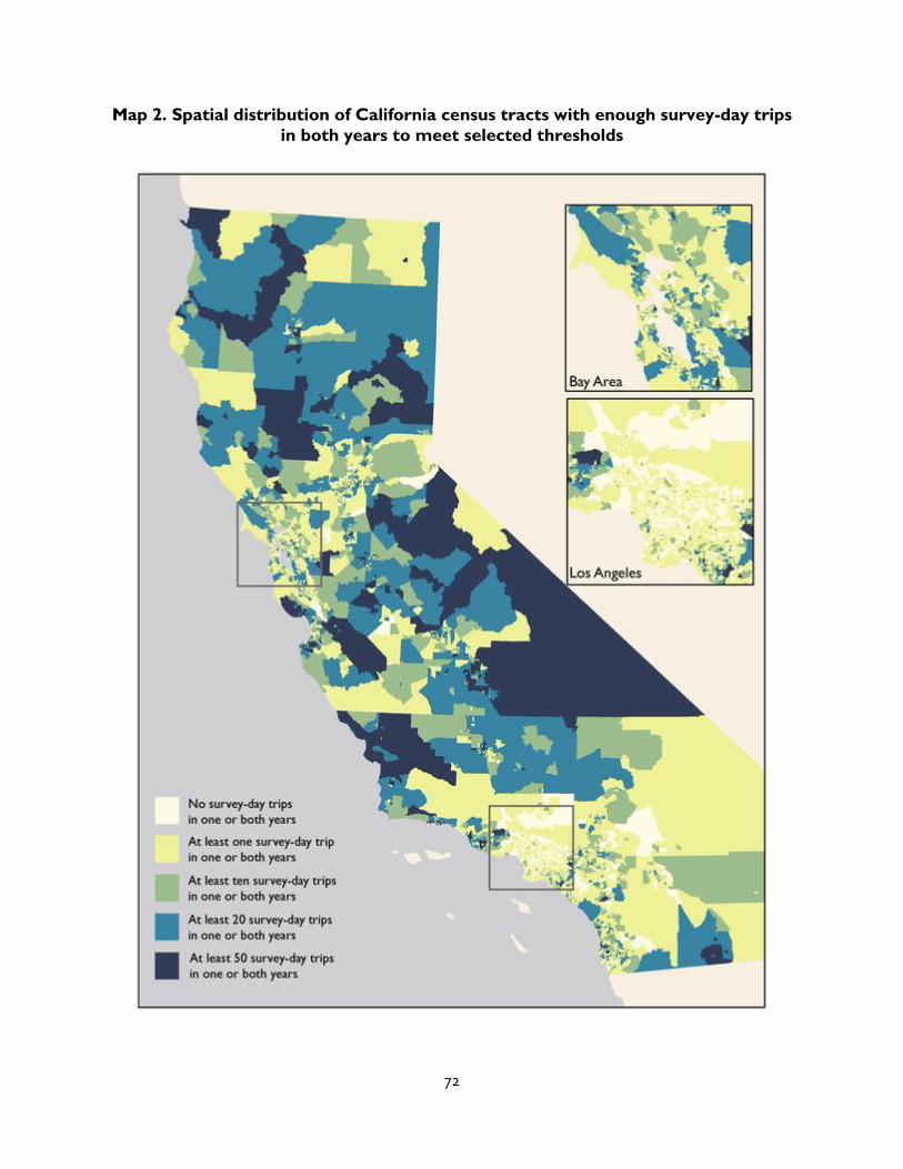
72
Map 2. Spatial distribution of California census tracts with enough survey-day trips
in both years to meet selected thresholds

73
Table 12. Number of California census tracts meeting selected thresholds for
survey-day trips 2001 CHTS 2012 CHTS Both Years
Number of census tracts in California (2010 boundaries) 8,057 8,057 8,057
Number of tracts with at least 1 survey-day trip origin 6,412 7,959 6,377
Number of tracts with at least 10 survey-day trip origins 2,951 6,609 2,783
Number of tracts with at least 20 survey-day trip origins 1,649 4,870 1,463
Number of tracts with at least 50 survey-day trip origins 575 1,884 429
In order to achieve a relatively large and diverse sample of census tracts while still using
meaningful estimates of walking mode share, we included all census tracts with at least 20
survey-day trip origins in our sample.
Throughout this paper, percent change for any census tract characteristic is calculated based on
the mid-point method, which yields values that can range from -200 percent to +200 percent:
𝑃𝑒𝑟𝑐𝑒𝑛𝑡 𝑖𝑛𝑐𝑟𝑒𝑎𝑠𝑒 = (𝑛𝑒𝑤 𝑣𝑎𝑙𝑢𝑒 − 𝑖𝑛𝑖𝑡𝑖𝑎𝑙 𝑣𝑎𝑙𝑢𝑒)
(12⁄ )(𝑛𝑒𝑤 𝑣𝑎𝑙𝑢𝑒 + 𝑖𝑛𝑖𝑡𝑖𝑎𝑙 𝑣𝑎𝑙𝑢𝑒)
Over the entire state, the walking mode share increased from 5 percent in 2001 to 9 percent in
2012, representing a 56 percent increase. Table 13 shows the changes in mode shares within
the sample tracts, and Figure 29 illustrates the distributions of the values in Table 13 and Map 3
shows the spatial distribution.
Table 13. Change in walking mode shares within sample tracts
Mean Median
2001 Walking mode share 5% 2%
2012 Walking mode share 8% 4%
Percent increase 45% 67%
For data on socioeconomic and housing characteristics of the census tracts in our sample, we
relied on data from the 2000 and 2010 United States Census, tabulated into consistent 2010
census boundaries by Logan, Xu, and Stults (2014). We obtained street network connectivity
data from Barrington-Leigh and Millard-Ball (2015). For some census tracts, the street network
was too sparse to calculate street network connectivity, and those tracts were excluded from
the sample, leaving a remaining sample of 1,303 census tracts. These tracts represent 16
percent of all census tracts in California and are home to 20 percent of the state’s population.
Our sample of census tracts is not representative of all California census tracts: the most
dense, urban census tracts appear to be the least likely to have been included in our sample.
However, as shown in Table 13, the walking mode shares and increases in walking within the
sample tracts and the increase in walking are comparable to those for the state overall.
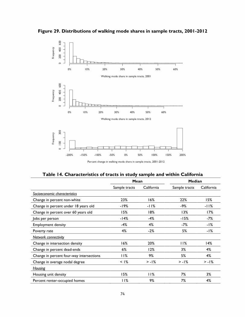
74
Figure 29. Distributions of walking mode shares in sample tracts, 2001-2012
Table 14. Characteristics of tracts in study sample and within California
Mean Median
Sample tracts California Sample tracts California
Socioeconomic characteristics
Change in percent non-white 23% 16% 22% 15%
Change in percent under 18 years old -19% -11% -9% -11%
Change in percent over 60 years old 15% 18% 13% 17%
Jobs per person -14% -4% -15% -7%
Employment density -4% 4% -7% -1%
Poverty rate 4% -2% 5% -1%
Network connectivity
Change in intersection density 16% 20% 11% 14%
Change in percent dead-ends 6% 12% 3% 4%
Change in percent four-way intersections 11% 9% 5% 4%
Change in average nodal degree < 1% > -1% > -1% > -1%
Housing
Housing unit density 15% 11% 7% 3%
Percent renter-occupied homes 11% 9% 7% 4%

75
Map 3. Percent change of walking mode shares in sample tracts, 2001-2012
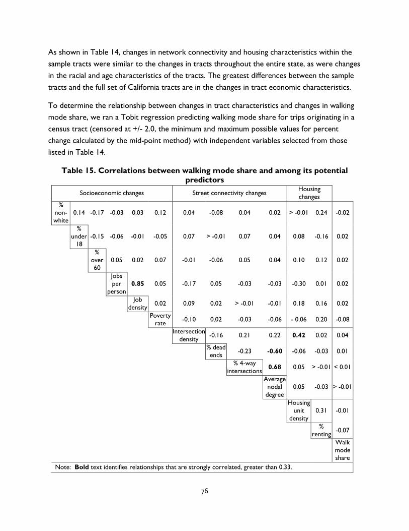
76
As shown in Table 14, changes in network connectivity and housing characteristics within the
sample tracts were similar to the changes in tracts throughout the entire state, as were changes
in the racial and age characteristics of the tracts. The greatest differences between the sample
tracts and the full set of California tracts are in the changes in tract economic characteristics.
To determine the relationship between changes in tract characteristics and changes in walking
mode share, we ran a Tobit regression predicting walking mode share for trips originating in a
census tract (censored at +/- 2.0, the minimum and maximum possible values for percent
change calculated by the mid-point method) with independent variables selected from those
listed in Table 14.
Table 15. Correlations between walking mode share and among its potential
predictors
Socioeconomic changes Street connectivity changes Housing
changes
%
non-
white
0.14 -0.17 -0.03 0.03 0.12 0.04 -0.08 0.04 0.02 > -0.01 0.24 -0.02
%
under
18
-0.15 -0.06 -0.01 -0.05 0.07 > -0.01 0.07 0.04 0.08 -0.16 0.02
%
over
60
0.05 0.02 0.07 -0.01 -0.06 0.05 0.04 0.10 0.12 0.02
Jobs
per
person
0.85 0.05 -0.17 0.05 -0.03 -0.03 -0.30 0.01 0.02
Job
density 0.02 0.09 0.02 > -0.01 -0.01 0.18 0.16 0.02
Poverty
rate -0.10 0.02 -0.03 -0.06 - 0.06 0.20 -0.08
Intersection
density -0.16 0.21 0.22 0.42 0.02 0.04
% dead
ends -0.23 -0.60 -0.06 -0.03 0.01
% 4-way
intersections 0.68 0.05 > -0.01 < 0.01
Average
nodal
degree
0.05 -0.03 > -0.01
Housing
unit
density
0.31 -0.01
%
renting -0.07
Walk
mode
share
Note: Bold text identifies relationships that are strongly correlated, greater than 0.33.

77
Table 15 shows the correlations among the variables considered for inclusion in the model,
with bold text to highlight correlations with a magnitude greater than 0.33. The model excludes
job density, housing unit density, percent dead ends, and percent four-way intersections, based
on their correlations with other variables.
Since both the dependent variables and all independent variables are expressed in terms of
percent change, the model coefficient estimates can be interpreted as elasticities: the percent
change in walking that would be anticipated for a one-percent change in the independent
variable.
Results
The results of the Tobit regression are summarized in Table 16. The model has an AIC score of
3917 and an R-squared value of 0.01. This suggests that only about one percent of the variation
in changes in walking mode shares in the sample census tracts can be explained by changes in
the built environment characteristics included in the model. This is not surprising; other studies
(including the research included in this report) show that trip, individual, and household
characteristics have a greater influence on mode choice than do neighborhood characteristics.
Moreover, reliable historical data on built environment characteristics that are likely to
influence walking mode choice —such as traffic congestion, the presence of sidewalks and
crosswalks, and quality of transit service— were not available for inclusion in the model.
Table 16. Results of Tobit regression model predicting change in walking mode
share
Estimated elasticity of walking
mode share
with respect to the variable
Standard
error
95-percent
confidence
interval P-value
Percent non-white 0.15 0.41 -0.65 to 0.96 0.713
Percent under 18 0.36 0.42 -0.46 to 1.17 0.394
Percent over 60 0.40 0.28 -0.15 to 0.96 0.154
Poverty rate -0.34 0.13 -0.59 to -0.10 0.007
Percent rental homes -0.40 0.29 -0.98 to 0.17 0.169
Jobs per person 0.15 0.15 -0.15 to 0.45 0.328
Intersection density 0.52 0.26 0.00 to 1.04 0.048
Average nodal degree -1.42 1.46 -4.27 to 1.44 0.331
Two coefficients are significant at a 95-percent confidence interval: the change in the poverty
rate and the change in intersection density. A one-percent increase in the poverty rate within a
census tract is associated with a 0.34-percent decrease in a census tract’s walking mode share.
A one-percent increase in the number of intersections per acre is associated with a 0.52-
percent increase in a census tract’s walking mode share.

78
Discussion of results
The negative elasticity of walking mode share with respect to the poverty rate may be
somewhat surprising, although the direction of the relationship is consistent with the findings
from the longitudinal study of regional statistical areas of Los Angeles by Joh et al. (2015), which
show a negative but statistically insignificant relationship between walking mode share and
household income.
The monetary cost of walking is minimal compared to the costs of vehicle ownership and
maintenance, or even compared to the cost of owning a bicycle or riding public transit. Thus,
one might expect residents of low-income neighborhoods to be the most likely to travel by
walking rather than by modes that incur greater monetary costs. Moreover, we calculated the
correlation between 2010 census tract poverty rates and current walking accessibility as
measured by Walk Score®, and found that neighborhood Walk Score® and neighborhood
poverty rates are positively correlated, with a Pearson correlation coefficient of 0.43.
However, while the monetary costs of walking may be the lowest, the time costs of walking are
the highest, since walking is the slowest mode. Many low-income neighborhoods are resource
poor, lacking in proximate opportunities easily reachable on foot such as available employment,
healthy food outlets, health-care services, social networks, and recreational facilities (Bostock,
2008; D’Angelo et al., 2011; Immergluck, 1998; Lovasi et al., 2009; Moore et al., 2008). Since
residents of low-income neighborhoods are likely to be constrained not only in terms of
money, but also in terms of time, greater reliance on motorized transportation may be a
necessity. These findings, however, may be influenced by the way in which we assembled the
data. Low-income adults are more likely to use transit than higher-income adults (Pucher &
Renne, 2003) and, therefore, we expect that they are also more likely to make walk trips to
access transit stops and stations (Besser & Danngenberg, 2005). However, short first- and last-
mile walk trips are excluded from our analysis since it focuses on linked trips taken to access an
ultimate destination.
The pedestrian environments in low-income neighborhoods may discourage walking. With
respect to the relationship between Walk Score® and poverty, Koschinsky et al. (2016)
compare Walk Score® with an alternative walkability index (the State of Place index) that
incorporates characteristics of the built environment that are not captured by Walk Score®,
including personal safety, traffic safety, and aesthetics. They find that the divergence between
Walk Score® and State of Place is greatest in low-income neighborhoods. Similarly, in their
study of low-income neighborhoods in New York, Neckerman et al. (2009:S264) find that poor
census tracts “had significantly fewer street trees, landmarked buildings, clean streets, and

79
sidewalk cafes, and higher rates of felony complaints, narcotics arrests, and vehicular crashes.”
Thus, low-income neighborhoods with high Walk Scores® may have less pedestrian-friendly
environments than high-income neighborhoods with the same Walk Scores®. Both Walk
Score® and State of Place are proprietary indices prepared and sold by for-profit firms
(Koschinsky et al., 2016).
The inverse relationship between walking mode shares and poverty rates may be partially
explained by perceptions of crime and safety in low-income neighborhoods. Studies show that
low-income women’s perceived lack of safety reduces their willingness to walk (Miles & Panton,
2006; Bennett et al., 2007). Participants in the Miles and Panton study expressed fears about
being assaulted or harassed or that passers-bys would fail to help them should a problem arise.
In a study of walking mode choice and crime rates in San Francisco, Ferrel et al. (2012) find that
the odds of walking are 17 percent lower for work trips and 61 percent lower for non-work
trips in high-crime areas, compared to low-crime areas. Yet, Joh et al. (2012) find that pro-
walking attitudes are more common in areas with high crime rates than in areas with low crime
rates. Together, these results may suggest that people living in neighborhoods with high crime
rates are especially likely to increase the share of trips they make by walking as the crime rates
in their neighborhoods decrease. However, no longitudinal studies have directly linked changes
in walking mode shares to changes in crime rates.
Thus, travel by a more leisurely mode such as walking may be a luxury that is more available to
residents of higher-income neighborhoods.
The elasticity of walking mode share with respect to intersection density is also statistically
significant and suggests that a one-percent increase intersection in density is associated with a
0.75 percent increase in walking. This is almost double the elasticity of 0.39 that Ewing and
Cervero (2010) find in their meta-analysis of seven cross-sectional studies that report a
relationship between walking and street or intersection density. Intersection density increases
the directness of walking routes, reducing walk trip distances and improving walking
accessibility.
Conclusion
The results of this analysis suggest two specific policy directions that show promise for further
increasing walking mode shares in neighborhoods throughout California.
First, despite research that suggests that residents of low-income neighborhoods have positive
attitudes towards walking, we find that walking mode shares have increased the most in
neighborhoods where the poverty rate has decreased. Thus, reducing poverty in California
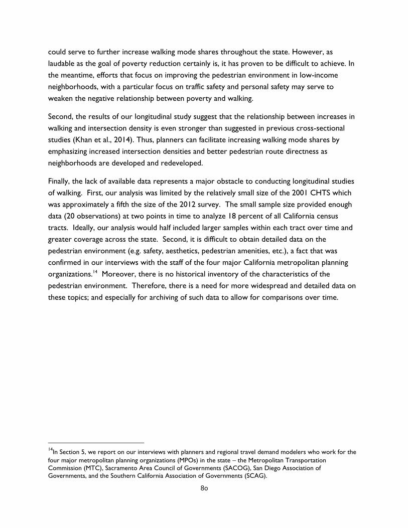
80
could serve to further increase walking mode shares throughout the state. However, as
laudable as the goal of poverty reduction certainly is, it has proven to be difficult to achieve. In
the meantime, efforts that focus on improving the pedestrian environment in low-income
neighborhoods, with a particular focus on traffic safety and personal safety may serve to
weaken the negative relationship between poverty and walking.
Second, the results of our longitudinal study suggest that the relationship between increases in
walking and intersection density is even stronger than suggested in previous cross-sectional
studies (Khan et al., 2014). Thus, planners can facilitate increasing walking mode shares by
emphasizing increased intersection densities and better pedestrian route directness as
neighborhoods are developed and redeveloped.
Finally, the lack of available data represents a major obstacle to conducting longitudinal studies
of walking. First, our analysis was limited by the relatively small size of the 2001 CHTS which
was approximately a fifth the size of the 2012 survey. The small sample size provided enough
data (20 observations) at two points in time to analyze 18 percent of all California census
tracts. Ideally, our analysis would half included larger samples within each tract over time and
greater coverage across the state. Second, it is difficult to obtain detailed data on the
pedestrian environment (e.g. safety, aesthetics, pedestrian amenities, etc.), a fact that was
confirmed in our interviews with the staff of the four major California metropolitan planning
organizations.14 Moreover, there is no historical inventory of the characteristics of the
pedestrian environment. Therefore, there is a need for more widespread and detailed data on
these topics; and especially for archiving of such data to allow for comparisons over time.
14
In Section 5, we report on our interviews with planners and regional travel demand modelers who work for the
four major metropolitan planning organizations (MPOs) in the state – the Metropolitan Transportation
Commission (MTC), Sacramento Area Council of Governments (SACOG), San Diego Association of
Governments, and the Southern California Association of Governments (SCAG).

81
References
Badland, H., & Schofield, G. (2005). Transport, Urban Design and Physical Activity: An Evidence-
Based Update. Transportation Research Part D, 10, 177–196.
Barrington-Leigh, C., & Millard-Ball, A. (2015). A Century of Sprawl in the United States.
Proceedings of the National Academy of Sciences of the United States of America, 112(27), 8244–
8249. http://doi.org/10.1073/pnas.1504033112
Bennett, G. G., McNeill, L. H., Wolin, K. Y., Duncan, D. T., Puleo, E., & Emmons, K. M. (2007).
Safe To Walk? Neighborhood Safety and Physical Activity Among Public Housing Residents.
PLOS Med, 4(10), e306. http://doi.org/10.1371/journal.pmed.0040306
Besser, L. M., & Dannenberg, A. L. (2005). Walking to Public Transit: Steps to Help Meet
Physical Activity Recommendations. American Journal of Preventive Medicine, 29(4), 273–280.
http://doi.org/10.1016/j.amepre.2005.06.010
Boarnet, M. G., Day, K., Anderson, C., McMillan, T., & Alfonzo, M. (2005). California’s Safe
Routes to School program: impacts on walking, bicycling, and pedestrian safety. Journal of the
American Planning Association, 71(3), 301–317.
Bostock, L. (2001). Pathways of Disadvantage? Walking as a Mode of Transport among Low-
Income Mothers. Health & Social Care in the Community, 9(1), 11–18.
Brown, B. B., Werner, C. M., Tribby, C. P., Miller, H. J., & Smith, K. R. (2015). Transit Use,
Physical Activity, and Body Mass Index Changes: Objective Measures Associated With
Complete Street Light-Rail Construction. American Journal of Public Health, 105(7), 1468–1474.
http://doi.org/10.2105/AJPH.2015.302561
Clifton, K. J., & Krizek, K. J. (2004). The Utility of the NHTS in Understanding Bicycle and
Pedestrian Travel (pp. 1–2). Presented at the National Household Travel Survey Conference:
understanding our nation’s travel.
D’Angelo, H., Suratkar, S., Song, H.-J., Stauffer, E., & Gittelsohn, J. (2011). Access to Food
Source and Food Source Use are Associated with Healthy and Unhealthy Food-Purchasing
Behaviours among Low-Income African-American Adults in Baltimore City. Public Health
Nutrition, 14(9), 1632–1639. http://doi.org/10.1017/S1368980011000498
Ewing, R., & Cervero, R. (2010). Travel and the Built Environment. Journal of the American
Planning Association, 76(3), 265–294.

82
Ferrell, C., Mathur, S., Meek, J., & Piven. (2012). Neighborhood Crime and Travel Behavior: An
Investigation of the Influence of Neighborhood Crime Rates on Mode Choice – Phase II (No. 11–4).
Mineta Transportation Institute Research Report. Retrieved from
http://transweb.sjsu.edu/project/2802.html
Freeland, A. L., Banerjee, S. N., Dannenberg, A. L., & Wendel, A. M. (2013). Walking Associated
with Public Transit: Moving Toward Increased Physical Activity in the United States. American
Journal of Public Health, 103(3), 536–542.
Goodman, A., Sahlqvist, S., & Ogilvie, D. (2014). New Walking and Cycling Routes and
Increased Physical Activity: One-And 2-Year Findings from the UK Iconnect Study. American
Journal of Public Health, 104(9), e38–e46.
Ham, S. A., Macera, C. A., & Lindley, C. (2005). Trends in Walking for Transportation in the
United States, 1995 and 2001. Preventing Chronic Disease, 2(4), A14.
Immergluck, D. (1998). Neighborhood Economic Development and Local Working: The Effect
of Nearby Jobs on Where Residents Work. Economic Geography, 74(2), 170–187.
http://doi.org/10.2307/144281
Joh, K., Chakrabarti, S., Boarnet, M. G., & Woo, A. (2015). The Walking Renaissance: A
Longitudinal Analysis of Walking Travel in the Greater Los Angeles Area, USA. Sustainability,
7(7), 8985–9011.
Joh, K., Nguyen, M. T., & Boarnet, M. G. (2012). Can Built and Social Environmental Factors
Encourage Walking among Individuals with Negative Walking Attitudes? Journal of Planning
Education and Research, 32(2), 219–236. http://doi.org/10.1177/0739456X11427914
Khan, M., M. Kockelman, K., & Xiong, X. (2014). Models for Anticipating Non-Motorized Travel
Choices, and the Role of the Built Environment. Transport Policy, 35, 117–126.
http://doi.org/10.1016/j.tranpol.2014.05.008
Koschinsky, J., Talen, E., Alfonzo, M., & Lee, S. (2016). How Walkable is Walker’s paradise?
Environment and Planning B: Planning and Design, 265813515625641.
http://doi.org/10.1177/0265813515625641
Logan, J. R., Xu, Z., & Stults, B. J. (2014). Interpolating U.S. Decennial Census Tract Data from
as Early as 1970 to 2010: A Longitudinal Tract Database. The Professional Geographer, 66(3),
412–420. http://doi.org/10.1080/00330124.2014.905156

83
Lovasi, G. S., Hutson, M. A., Guerra, M., & Neckerman, K. M. (2009). Built Environments and
Obesity in Disadvantaged Populations. Epidemiologic Reviews, 31, 7–20.
http://doi.org/10.1093/epirev/mxp005
MacDonald, J. M., Stokes, R. J., Cohen, D. A., Kofner, A., & Ridgeway, G. K. (2010). The Effect
of Light Rail Transit on Body Mass Index and Physical Activity. American Journal of Preventive
Medicine, 39(2), 105–112.
McCormack, G. R., & Shiell, A. (2011). In Search Of Causality: A Systematic Review of the
Relationship Between the Built Environment and Physical Activity Among Adults. International
Journal of Behavioral Nutrition and Physical Activity, 8(1), 125. http://doi.org/10.1186/1479-5868-8-
125
McKenzie, B. (2014). Modes Less Traveled—Bicycling and Walking to Work in the United
States: 2008–2012. US Census Bureau, New York.
Miles, R., & Panton, L. (2006). The Influence of the Perceived Quality of Community
Environments on Low-Income Women’s Efforts to Walk More. Journal of Community Health,
31(5), 379–392. http://doi.org/10.1007/s10900-006-9021-9
Moore, L. V., Diez Roux, A. V., Evenson, K. R., McGinn, A. P., & Brines, S. J. (2008). Availability
of Recreational Resources in Minority and Low Socioeconomic Status Areas. American Journal of
Preventive Medicine, 34(1), 16–22. http://doi.org/10.1016/j.amepre.2007.09.021
Neckerman, K. M., Lovasi, G. S., Davies, S., Purciel, M., Quinn, J., Feder, E., Raghunath, N.,
Wasserman, R., Rundle, A. (2009). Disparities in Urban Neighborhood Conditions: Evidence
from GIS Measures and Field Observation in New York City. Journal of Public Health Policy, 30
Suppl 1, S264-285. http://doi.org/10.1057/jphp.2008.47
Ogilvie, D., Foster, C. E., Rothnie, H., Cavill, N., Hamilton, V., Fitzsimons, C. F., Mutrie, N.,
Scottish Physical Activity Research Collaboration. (2007). Interventions to Promote Walking:
Systematic Review. Bmj.
Pucher, J., Buehler, R., Merom, D., & Bauman, A. (2011). Walking and Cycling in the United
States, 2001–2009: Evidence from the National Household Travel Surveys. American Journal of
Public Health, 101(S1), S310–S317.
Pucher, J., & Renne, J. (2001). Socioeconomics of Urban Travel: Evidence from the 2001 NHTS.
Transportation Quarterly, 57(3). Retrieved from
https://www.researchgate.net/publication/235359454_Socioeconomics_of_Urban_Travel_Evide
nce_from_the_2001_NHTS

84
Saelens, B. E., & Handy, S. L. (2008). Built Environment Correlates of Walking: A Review.
Medicine and Science in Sports and Exercise, 40(7 Suppl), S550–S566.
Santos, A., McGuckin, N., Nakamoto, H. Y., Gray, D., & Liss, S. (2011). Summary of Travel
Trends: 2009 National Household Travel Survey (No. FHWA-PL-ll-022). Federal Highway
Administration. Retrieved from https://trid.trb.org/view.aspx?id=1107370
Simpson, M. E., Serdula, M., Galuska, D. A., Gillespie, C., Donehoo, R., Macera, C., & Mack, K.
(2003). Walking trends among US adults: the behavioral risk factor surveillance system, 1987–
2000. American Journal of Preventive Medicine, 25(2), 95–100.
Stopher, P. R., & Greaves, S. P. (2007). Household Travel Surveys: Where are we going?
Transportation Research Part A: Policy and Practice, 41(5), 367–381.
Tudor-Locke, C., Van Der Ploeg, H. P., Bowles, H. R., Bittman, M., Fisher, K., Merom, D.,
Gershuny, J., Bauman, A., Egerton, M. (2007). Walking Behaviours from the 1965–2003
American Heritage Time Use Study (AHTUS). International Journal of Behavioral Nutrition and
Physical Activity, 4(1), 45.

85
V. Strutting into practice: Walking and travel demand modeling
Introduction
As previously extolled throughout this report, walking is a good way for people to travel.
Traveling by foot produces no greenhouse gas emissions, adds no congestion to the street or
highway network, and is good for individual and public health (Frank et al., 2004; Murphy et al.,
2007). Given these individual and societal benefits, cities, regional governments and
metropolitan planning organizations have been working to increase the number of trips
completed by walking. Enthusiasm toward walking has been aided by substantial increases in
federal investments in active transportation – bicycling and walking (Fields & Cradock, 2015).
National data show an increase in walking rates (Ham et al., 2005; Joh et al., 2015; Pucher et al.,
2011; Simpson et al., 2003; Tudor-Locke et al., 2007). Walking also has increased in California.
As noted in previous chapters, the walking mode share in the four primary metropolitan
statistical areas in California increased from 5 to 9 percent from 2001to 2012. As Figure 30
shows, and as previously described in Chapter 3, this growth has been related to two principal
factors: (1) changes in the characteristics of the population and the communities in which they
live and (2) changes in the effects of these characteristics on the likelihood of walking.
Given the benefits of and the increase in walking, metropolitan planning organizations (MPOs)
would be wise to understand and incorporate walking into their analyses of regional travel to
adequately plan for their regions. To what extent do MPOs already do this? More specifically,
for this research, we examine how regional travel demand models—models that estimate the
expected demand for transportation infrastructure—include walking and the factors related to
this mode of travel.

86
Figure 30. Increase in walking attributable to changes in trip, individual, household,
and neighborhood characteristics
As other scholars highlight, travel demand models often inadequately incorporate walking. In
fact, many regional models in the United States do not forecast non-motorized travel at all
(Singleton & Clifton, 2013). Singleton and Clifton (2013) reviewed the modeling framework for
the 48 largest MPOs serving greater than one million people. The authors organized the MPOs
into six categories. At the very top are MPOs that assigned walk and bicycle trips to the
network; at the very bottom are those MPOs that do not model non-motorized travel.
According to their framework, the MPOs in our study area (Bay Area, Sacramento, Los Angeles
and San Diego) all do a reasonably good job of incorporating walking into their modeling
efforts.
This study builds on the work of Singleton and Clifton (2013) through in-depth interviews with
the four major Metropolitan Planning Organizations (MPOs) in California; the Metropolitan
Transportation Commission (MTC), San Diego Association of Governments (SANDAG),
Sacramento Area Council of Governments (SaCOG) and the Southern California Association of
Governments (SCAG). All four MPOs were categorized near the top of Singleton and Clifton’s
(2013) spectrum.
Change in trip
characteristics
25%
Changes in individual characteristics
7%
Changes in
household
characteristics
4%Changes in
neighborhood
characteristics
10%
Changes in relative
MSA populations
13%
Changes in effects of
trip, household, and
neighborhood
characteristics
41%

87
Our research focuses on the following three questions:
1. How do current approaches to travel demand modeling incorporate walking behavior
and pedestrian infrastructure?
2. How sensitive are travel demand models to changes in walking behavior and factors
associated with walking behavior?
3. What, if any, improvements should be made to regional travel demand models to better
integrate and understand walking?
We find that activity-based travel demand models are better suited to incorporating walking
trips than the traditional four-step modeling approach. Three of the four15 MPOs currently use
activity-based models. However, even this approach can be strengthened with respect to the
walking component of the models. Our interviews reveal the following and suggest potential
improvements relate to five broad themes:
Quality of mode choice data: Household travel surveys, the common building block
for regional travel demand models, tend to underrepresent walking.
Quality of the modeled relationship between capacity and demand: The demand
for walking and the capacity to accommodate this mode of travel are different for
walking than for other modes. Regional travel demand models largely are used to make
large infrastructure decisions and to shape regional transportation policy. As currently
structured, they are not as useful in understanding and in making decisions regarding
investments necessary to induce or improve walking.
Quality of infrastructure data: There is no systematic inventory of the walking
network and the quality of pedestrian infrastructure. As such, MPOs are hard pressed
to quickly pinpoint where the pedestrian network needs to be improved.
Geographic coarseness of large-scale models: Models are built to understand
responses to larger-scale (e.g. regional) policies and projects than those that are
necessary to induce or improve walking (which are more likely to be at the
neighborhood level).
Quality of route choice data: There are limited data on walking, particularly as it
relates to the geography of walk trips. This gap inhibits model calibration and makes it
difficult to identify specific intersections or corridors on the network where pedestrian
volumes are likely to be high.
15
SCAG, the only MPO not currently using an activity-based model, has one in development and reports to be
making the switch within the next regional transportation plan update.

88
We expand on these themes as follows. We first define travel demand models, drawing from
the literature on their purposes and relative merits. We then the approach we took in our
interview process. We draw on these interview data in developing our major findings. Finally,
the chapter concludes with a discussion of how planning agencies can improve their
understanding of walking in the context of regional travel models.
Travel demand models: The basics
Travel demand models are tools to understand how current travel and future travel will be
distributed across a regional network. They seek to answer questions such as: how many more
trips can be expected due to population growth, where will those trips be located, and how will
travel be distributed across different modes? As travel demand grows, the network must
accommodate this growth. Consequently, Metropolitan Planning Organizations (MPOs) use the
output of travel demand models to make decisions about transportation investments to best
meet future needs.
To provide accurate predictions, travel demand models must accurately represent how people
travel. Trips are assigned to the transportation network which, therefore, requires modelers
to have accurate and detailed knowledge of the network. For example, they must have
information on such elements as: the number of lanes on any particular street in the network,
the number of turning lanes and the signal phasing, the length of highway on-ramps, etc. The
modelers synthesize the location of people and their associated demographic characteristics,
employment, and housing across the region. Travel demand modelers rely on these data to
perform complex scenarios to simulate regional travel.
The model output is then used to develop potential scenarios related to future travel patterns
and air quality, and to plan future infrastructure projects. For example, planners are interested
in the potential answers to the following types of questions. How will travel shift if additional
infill housing is created in certain locations? How will travelers likely respond to a new toll lane?
If there is new transit service, from where will riders come? Planners can forecast future
scenarios based on potential changes in the population, the transportation network, and the
built environment.
There are two basic model types. The four-step trip-level model remains the dominant
approach still used by most MPO’s (Clifton et al., 2016). Activity-, tour-based modeling is a
newer approach that provides a more representative understanding of individual daily travel
(National Academies of Sciences, 2015). Trip-level models identify origins and destinations and
assign trips to those locations. In contrast, tour-level models simulate travelers as they use the
system and conduct all of their daily activities. The decisions this traveler makes are constrained

89
by the number and type of activities and the available modes. In a trip-level approach, the model
could estimate that 85% of trips at a particular employment location will be by driving. Using
the tour- and activity-based approach, the number of trips by car at that location would depend
on how many people arrived by car on that particular day. As described by one of our
interviewees, the two model approaches should not produce different results at the macro
level but rather, activity-based models provide a much greater level of detail. Drawing on the
analogy of watching a television show in black and white versus color, one of our interviewees
explained “it’s still the same show. You just have a lot more nuance to what you're seeing.”
While the two model types may produce similar overall results, activity-based approaches are
generally viewed as the superior approach, particularly for walking (Davidson et al., 2007,
Cervero, 2006, Singleton & Clifton, 2013, Clifton et al., 2016). Activity-based models
understand walking is derived from an inherent need to perform individual and household
activities. Thus, these models understand travel for more purposes than the commute; which
we previous demonstrated is one of the least likely walking trip types. Secondly, activity-based
models take into account travel trade-offs between members of a household, such as
coordinating household vehicles. We similarly previously demonstrated how vehicle availability
affects the choice to make trips by walking.
More generally, significant improvements in activity-based approaches include linking activities
and travel, understanding time and space restrictions and incorporating characteristics of
individuals into the decision-making process. Further, mode choices are constrained to a
plausible range of options. For example, activity-based models assume that if a person did not
travel by a car when they left on their first trip of the morning, this individual does not have a
vehicle available for other trips during that day. Trips are not independent of each other; rather
people have chains of trips, known as tours, and complete their necessary travel within those
tours.
Limited technical and staff resources often hinder MPOs from moving to activity-based model
approaches. Clifton and Singleton (2013) review the modeling approaches of the 48 largest
MPOs in regions with populations greater than one million. They find that the four MPOs in
our study areas all consider walking trips at some point in the modeling process and, in
comparison to other large MPOs, give greater consideration to this mode. Our interviews build
on this research by developing an in depth understanding of where additional improvements are
required.
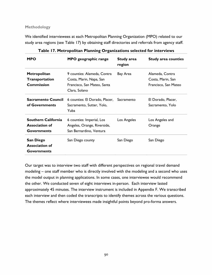
90
Methodology
We identified interviewees at each Metropolitan Planning Organization (MPO) related to our
study area regions (see Table 17) by obtaining staff directories and referrals from agency staff.
Table 17. Metropolitan Planning Organizations selected for interviews
MPO MPO geographic range Study area
region
Study area counties
Metropolitan
Transportation
Commission
9 counties: Alameda, Contra
Costa, Marin, Napa, San
Francisco, San Mateo, Santa
Clara, Solano
Bay Area Alameda, Contra
Costa, Marin, San
Francisco, San Mateo
Sacramento Council
of Governments
6 counties: El Dorado, Placer,
Sacramento, Sutter, Yolo,
Yuba
Sacramento El Dorado, Placer,
Sacramento, Yolo
Southern California
Association of
Governments
6 counties: Imperial, Los
Angeles, Orange, Riverside,
San Bernardino, Ventura
Los Angeles Los Angeles and
Orange
San Diego
Association of
Governments
San Diego county San Diego San Diego
Our target was to interview two staff with different perspectives on regional travel demand
modeling – one staff member who is directly involved with the modeling and a second who uses
the model output in planning applications. In some cases, one interviewee would recommend
the other. We conducted seven of eight interviews in-person. Each interview lasted
approximately 45 minutes. The interview instrument is included in Appendix F. We transcribed
each interview and then coded the transcripts to identify themes across the various questions.
The themes reflect where interviewees made insightful points beyond pro-forma answers.

91
Improving walking in regional travel demand forecasts in major California regions
Quality of mode choice data
Household travel surveys are the primary input for information about trip making in the travel
demand models. The surveys provide information about how far people travel, by which mode,
and for what purpose. In turn, these data help to understand household trip generation and,
further, to help understand the dynamic relationships among travel patterns, demographics, and
land use. After the model is developed, household travel survey data provide a reference point
for model validation.
Some interviewees voiced concern about these data. Sample sizes are small and the data can
only be as good as the participant’s memory and record keeping. One interviewee states:
“We are kind of comparing our data to make sure our assumptions are
reasonable especially when we have sketchy data sources, which the household
travel survey usually are.”
Their comments echo the critiques of other scholars. For example, Wolf et al. (2003) estimate
that travel surveys underreport as much as 60% of trips, with the majority of these fairly short
trips. Walking trips are short; in our four metropolitan areas the average walk distance is about
½ a mile and has declined over time (See Chapter 3 for a discussion of changes in trip distance
from 2001 to 2012). Since walking trips are the shortest, concerns about general non-
representation of travel in the survey data are likely much worse for walking trips (Houston, et
al., 2014).
Regional demand models can only accurately estimate travel if reliable travel patterns are
reflected in the household survey data. Monitoring the household travel survey process is
essential to ensuring the accuracy of regional models.
The California Department of Transportation (Caltrans) greatly increased the sample size of
the most recent statewide household travel survey. While a larger sample does not correct for
the under-reporting of walk trips, it provides greater representation of the population, limits
the influence of outliers, and allows for analysis of statistical difference. As noted in Table 18
the number of households with completed travel diaries more than doubled between the 2001
and 2012 surveys.

92
Table 18. Number of households between CA travel survey years
Survey Year Households
2001 17,040
2012 42,431
As explained by Stecher et al. (2014), the existence of a pooled funding consortium between
state agencies and eight regional partners increased the budget allocated to the survey, leading
to a larger sample size. Further, this partnership allowed for the use of a more comprehensive
survey instrument than any of the regions would have been able to produce on their own. In
the future, conducting these surveys as a collaborative state-wide effort would lead to more
detailed, reliable data on walking. Such data would help local regional and state agencies to
better understand trends in walking and the factors that influence them.
Quality of the modeled relationship between capacity and demand
Regional travel demand models serve, first and foremost, a federal statutory purpose:
conformity with the federal Clean Air Act. Additionally, interviewees spoke about a second and
related purpose, the importance of having a tool for measuring how future projects or packages
of projects will perform. One interviewee stated:
“The RTP [regional transportation plan] process requires you to have some kind
of modeling framework in order to evaluate the outcomes of your
investments”
Another interviewee commented:
“You’re making a lot of decisions in the present about investments and policies
that will influence the future in a big way in theory. And you want to base those
decisions in the here and now on the best information you can bring...So the
travel models fill that void….[the model] creates information that is not really
available in the real world and it fills in for a lot of that information needed for
people who have to make decisions now.”
One interviewee provided an explanation for the lack of attention to walking: “We have to
keep the travel model relevant to the policy questions that are being asked.”
The use of regional models to plan investments may work better for motorized traffic and, to a
lesser extent, for bicycling compared to walking since traveler response to changes in
infrastructure are fairly well understood. MPOs can use model results to forecast the number
of people likely to use a transit line or a particular transit station. Similarly, these models can
93
help forecast traveler responses to tolling or travel demand management strategies (National
Academies of Sciences, 2006; Davidson et al., 2007).
However, interviewees recognized that the decision to walk is likely to be based on a wider
variety of factors than simple cost and travel time. Thus, the causal links between the decision
to make a walk trip and capacity of the pedestrian network is quite weak —particularly when
pedestrian infrastructure is represented at the level of detail that is typical for regional travel
demand models.
Walking trips are less strongly linked to infrastructure availability than all other modes. For
example, a car or transit vehicle cannot travel on a street without a lane; but someone could
walk on a street without a sidewalk.
In the meta-review of the built environment and walking, only four studies correlated walking
to sidewalks (Saelens & Handy, 2008). More studies found relationships between both
aesthetics and accessibility than sidewalks.
Can the model answer relevant policy questions specific to walking? For example, can regional
travel demand models give a reasonable estimate for how many more people will walk if a
sidewalk is installed or improved?
In short, the answer is no. Interviewees noted that walking trips are linked to areas of higher
density, with a greater number of destinations in close proximity to large amounts of people
and a connected street grid as determinates of walking. The availability of sidewalks may matter
in these cases, but interviewees did not believe that they are not the driving force.
Interviewees asserted that without a simple link between infrastructure and demand, MPOs are
likely to find it difficult to use these regional travel demand tools for evaluating and ranking
different policy questions about walking. They commented:
“So are we capturing the value of investments in amenities on the pedestrian
side? Probably not.”
“This time for the first time, we’ll be assigning bike trips and ped trips will be
locating them on the network. But then the question, is ok, are we assigning
them Are we assigning them in the right place? We still don’t have great data
sources on either side to know. The bike data is getting better. And the ped
data, we’ll likely just look at [the output] to make sure people are walking more
in the places we expect them to be walking more.”

94
The weak causal link between the demand for walk trips and the capacity of the pedestrian
network is not the only obstacle to applying regional travel demand models to understanding
walking trip rates and walking mode choice. Gaps in representations of the walking network
and the large scale of the models’ geographic units of analysis are additional issues. We further
explain these issues in the following sections.
Quality of infrastructure data
Travel demand models also have difficulty predicting walk trips because of gaps in
representation of the walking network. Imagine opening your navigation system in a car and
finding no roadmap. You would be lost. You would think, ‘how can I get to my destinations
without knowing where the streets are located?’ While information about the road network is
widely available, information about characterizing the pedestrian network is not. The lack of
information on the walking network hinders the ability of modelers to assign walking trips to
particular locations.
MPOs have to assemble information about the pedestrian network throughout the region. Data
about the roadway network can be purchased by any number of third-party navigation
companies. Transit information can be accessed through the nationwide Google Transit Feed
Specification (for most places) or directly from transit operators. Finally, cities often have
geographic data on the bicycling network. From where does information about the pedestrian
network come?
As our interviewees note, in general, MPOs are missing these data:
“The missing part is the infrastructure for walking. It is very difficult to get the
sidewalk information to reflect infrastructure”
“We don’t know how many of those streets have sidewalks. We don’t have
[data on] how many of those streets have a landscape strip that buffers a
pedestrian from noise on the street or perceived safety on the street, or
whatever. So we have a street pattern variable which influences walking but we
don’t have anything that’s a true pedestrian environment variable.”

95
Some MPOs have a basic representation of the sidewalk network. However, are sidewalks the
only information relevant to understanding walking? Studies suggest that other characteristics
of the walking environment may be important such as land use mix, density of destinations,
small blocks and high intersection density (Cervero & Duncan, 2003; Saelens & Handy, 2007).
Understanding these relationships is important for the allocation of scarce transportation
dollars to improve the pedestrian environment. MPOs should not wait to allocate funds until
they have developed a detailed pedestrian network. But they ought to develop better and
more fine-grained approaches to representing the walking network.
Geographic coarseness of large-scale models
As suggested by the name, regional travel demand forecasting models generate information
about large areas. In the case of the Southern California MPO, SCAG, the region covers 38,000
square miles. Regions must be sub-divided into smaller parts; the most common sub-regional
units used for this purpose are “traffic analysis zones” (TAZs). TAZ boundaries are generally
designated by the MPO with the intention that they should be small enough that most trips
occur between TAZs, rather than within TAZs, since within-TAZ trips are not assigned to the
network. Thus, the geographic area of a TAZ will be a function of the typical expected length of
trips beginning and ending there. As a result, TAZs are large in sprawling outlying areas and
small in dense urban cores as each unit tries to each represent generally the same amount of
information and are generally akin to the size of a census tract.
Regional demand models generate travel intensities at this geographic level and further attempt
to assign trips to the network itself. MPOs have improved their models by increasing the total
number of TAZs and reducing their size. For example, in the Bay Area, MTC’s next model
iteration will have a 60-fold increase in the number of TAZs. An interviewee from this region
explained:
“Our current model has 1450 TAZs. The next version will have 60,000 so that is a 60x
increase. And once you do that, there’s a lot of things that just change in how you
represent behaviors because you have a lot more detail.”

96
But is this spatial unit of analysis—the TAZ—appropriate for understanding walking? Smaller
units help to more accurately reflect the location of built environment characteristics. Think of
a neighborhood with a dense commercial corridor and single family homes. If this neighborhood
is one large area, access to these destinations will be averaged over the entire neighborhood. In
reality, people further away from the destinations are less likely to walk compared to residents
who are more proximate to these commercial destinations. Smaller units allow for a more
nuanced depiction of the built environment and, therefore, are better at capturing and
describing short distance trips made by foot.
Quality of route choice data
A final obstacle to incorporating walking into regional travel demand models is the absence of
pedestrian volume data at the intersection level. Transportation agencies at the local, regional,
and state levels routinely collect vehicular traffic volume data. Traffic volume data can be used
to calibrate regional travel demand models so they can accurately reflect drivers’ route choice
decisions. For example, at what point will congestion delays cause drivers to divert to less
direct routes? Absent this information, the travel demand model could indicate approximately
how many vehicles travel from one part of the region to another, but could not indicate which
roadways they would use and where additional capacity might be needed.
Our interviews indicate that, across all regions, MPOs are operating their travel demand
models without adequate data that would allow them to calibrate their models to accurately
assign pedestrian trips to their most likely routes. The household travel survey can provide a
general picture of how much overall walking occurs in the region and even within specific areas.
However, this survey does not provide information about which paths and intersections
pedestrians use. As a result, even in the case where a TAZ is the size of one city block, no
information exists as to where a particular safety improvement should be located in that space
to maximize its effect.
This deficiency highlights the difficulty in using regional travel demand models to assess future
projects’ effects on travel. And further, the main point of concern for MPOs to understand
walking may not lie in the modeling approach itself; whether basic or sophisticated four step or
the more advanced activity based approaches. Rather, the lack of a complete picture of walking,
from the incomplete network representation to the intensity at specific intersections, places
this mode at a major disadvantage in this key decision support tool.
97
Discussion and conclusion
Walking is a simple way to get around, but modeling this simple mode is quite complicated.
While the major California MPOs are doing a better job of analyzing walking than most large
MPOs in other parts of the country, there is much room for improvement.
Since regional travel demand models are often the basis for allocating funds for future
transportation investments, improvements to walking infrastructure are at a disadvantage
because obstacles to walking go far beyond a lack of capacity, and include factors such as
comfort and safety that are difficult, and perhaps impossible, to incorporate into large-scale
regional models. Nothing in the modeling framework is going to correct for this problem.
However, an awareness of this conundrum where one mode is distinctly different than others
may have the potential to begin addressing this issue.
Based on the results of our interviews, we recommend four distinct ways to improve how
regional governments understand and plan for walking:
1. State and regional agencies ought to continue to support statewide efforts to collect
household travel data
Similar to a popular television commercial, we also believe more is better. If more
households complete the survey, the dataset will include more trips. A larger dataset
will help to seed the regional models with more information about diverse types of
trips. The resulting model results are likely to be more accurate if they have a richer
dataset as their foundation.
A continued partnership between state and regional agencies may provide the resources
necessary to explore other data collection strategies. For example, collecting data via
GPS rather than by survey and individual recall will likely improve the accuracy of the
data, particularly for short trips and/or trips that are taken only occasionally.
2. Develop and maintain a dataset on sidewalks
Travel demand models are only as good as the information that goes into them. Most of
the MPOs do not have basic information about the availability of sidewalks. This is not
uncommon, since municipalities often struggle to build and maintain this type of a
dataset (Grossman et al., 2014). Sidewalks are the most basic component of walking
infrastructure. Thus, governments need to have information about their quality and
allocation.

98
As rates of walking continue to increase, sidewalk availability and quality will be
increasingly important. Regional transportation plans and funding can assist in improving
sidewalk allocation and quality. However, to do so, planners must have information on
where people walk and identify infrastructure problems.
3. Collect information about pedestrian locations and volumes across the region
None of our MPOs were able to confidently validate their model output for walking
trips. This again puts walking at a disadvantage because MPOs may not be able to
identify where people walk and plan for safety improvements.
Understandably, collecting pedestrian volume data is not as simple as collecting vehicle
data. Cities cannot lay down a tube across the sidewalk akin to how car traffic data are
collected. But the technology for collecting pedestrian data is quickly improving. MPOs
should pay close attention to these new technologies and potentially incorporate them
into other traffic volume data collection efforts.
4. Continue to exchange ideas about modeling improvements
Many of the interviewees knew each other. They also noted the information exchange
that occurs between MPOs, particularly MPOs in close proximity. As previously
referenced by Singleton and Clifton (2013), the MPOs in our study areas are some of
the national leaders in forecasting pedestrian behavior. Continual collaboration between
these forward-thinking MPOs can potentially enhance efforts to better plan for walking.
Further, these leaders can assist other smaller MPOs that may be less advanced in their
representation of walking and non-motorized travel behavior.
99
References
Cervero, R. (2006). Alternative Approaches to Modeling the Travel-Demand Impacts of Smart
Growth. Journal of the American Planning Association, 72(3), 285–295.
http://doi.org/10.1080/01944360608976751
Cervero, R., & Duncan, M. (2003). Walking, Bicycling, and Urban Landscapes: Evidence From
the San Francisco Bay Area. American Journal of Public Health, 93(9), 1478–1483.
Clifton, K. J., Singleton, P. A., Muhs, C. D., & Schneider, R. J. (2016). Representing Pedestrian
Activity in Travel Demand Models: Framework and Application. Journal of Transport Geography,
52, 111–122. http://doi.org/10.1016/j.jtrangeo.2016.03.009
Davidson, W., Donnelly, R., Vovsha, P., Freedman, J., Ruegg, S., Hicks, J., Castiglione, J., Picado,
R. (2007). Synthesis of First Practices and Operational Research Approaches in Activity-Based
Travel Demand Modeling. Transportation Research Part A: Policy and Practice, 41(5), 464–488.
http://doi.org/10.1016/j.tra.2006.09.003
Fields, B., & Cradock, A. L. (2014). Federal Active Transportation Policy in Transition: From
ISTEA to Complete Streets. Public Works Management & Policy, 19(4), 322–327.
http://doi.org/10.1177/1087724X14546200
Frank, L. D., Andresen, M. A., & Schmid, T. L. (2004). Obesity Relationships with Community
Design, Physical Activity, and Time Spent in Cars. American Journal of Preventive Medicine, 27(2),
87–96.
Grossman, A., Elango, V., Frackelton, A., & Guensler, R. (2014). Use of Sidewalk Quality
Assessment Survey in Developing Sidewalk Ratings. In Proceedings from the 2014 Transportation
Research Board Annual Meeting. Washington, D.C.: National Academies of Science. Retrieved
from http://amonline.trb.org/trb-59976-2014-1.2467145/t-1132-1.2479434/564-1.2476794/14-
4933-1.2479477/14-4933-1.2479480
Ham, S. A., Macera, C. A., & Lindley, C. (2005). Trends in Walking for Transportation in the
United States, 1995 and 2001. Preventing Chronic Disease, 2(4), A14.
Houston, D., Luong, T. T., & Boarnet, M. G. (2014). Tracking Daily Travel; Assessing
Discrepancies between GPS-Derived and Self-Reported Travel Patterns. Transportation Research
Part C: Emerging Technologies, 48, 97–108. http://doi.org/10.1016/j.trc.2014.08.013
100
Joh, K., Chakrabarti, S., Boarnet, M. G., & Woo, A. (2015). The Walking Renaissance: A
Longitudinal Analysis of Walking Travel in the Greater Los Angeles Area, USA. Sustainability,
7(7), 8985–9011.
Murphy, M. H., Nevill, A. M., Murtagh, E. M., & Holder, R. L. (2007). The Effect of Walking on
Fitness, Fatness and Resting Blood Pressure: A Meta-Analysis of Randomised, Controlled Trials.
Preventive Medicine, 44(5), 377–385. http://doi.org/10.1016/j.ypmed.2006.12.008
National Academies of Sciences. (2006). Estimating Toll Road Demand and Revenue (NCHRP
Synthesis No. 364). Washington, D.C.: National Cooperative Highway Research Program.
Retrieved from http://www.trb.org/Publications/Blurbs/158707.aspx
National Academies of Sciences. (2015). Activity-Based Travel Demand Models: A Primer. Retrieved
from http://www.nap.edu/catalog/22357/activity-based-travel-demand-models-a-primer
Pucher, J., Buehler, R., Merom, D., & Bauman, A. (2011). Walking and Cycling in the United
States, 2001–2009: Evidence from the National Household Travel Surveys. American Journal of
Public Health, 101(S1), S310–S317.
Saelens, B. E., & Handy, S. L. (2008). Built Environment Correlates of Walking: A Review.
Medicine and Science in Sports and Exercise, 40(7 Suppl), S550–S566.
Simpson, M. E., Serdula, M., Galuska, D. A., Gillespie, C., Donehoo, R., Macera, C., & Mack, K.
(2003). Walking Trends among US Adults: The Behavioral Risk Factor Surveillance System,
1987–2000. American Journal of Preventive Medicine, 25(2), 95–100.
Singleton, P. A., & Clifton, K. J. (2013). Pedestrians in Regional Travel Demand Forecasting
Models: State of the Practice. Presented at the Transportation Research Board 92nd Annual
Meeting. Retrieved from https://trid.trb.org/view.aspx?id=1242847
Stecher, C., Chesbro, S., & Zhang, Y. (2014). Herding Tigers: Lessons Learned from California
Household Travel Survey. In Proceedings from the 2013 Transportation Research Board Annual
Meeting. Washington, D.C.: National Academies of Science. Retrieved from
http://amonline.trb.org/trb-59976-2014-1.2467145/t-1112-1.2488871/378-1.2490420/14-2300-
1.2490482/14-2300-1.2490484
Tudor-Locke, C., Van Der Ploeg, H. P., Bowles, H. R., Bittman, M., Fisher, K., Merom, D.,
Gershuny, J., Bauman, A., Egerton, M. (2007). Walking Behaviours from the 1965–2003
American Heritage Time Use Study (AHTUS). International Journal of Behavioral Nutrition and
Physical Activity, 4(1), 45.

101
Wolf, J., Loeschl, M., Myers, J., & Arce, C. (2003). Trip Rate Analysis in GPS-Enhanced Personal
Travel Surveys. In Transport Survey Quality and Innovation (pp. 483–498). London: Pergamon.
Retrieved from http://books.emeraldinsight.com/display.asp?K=9780080440965

102
Appendix A. Studies on changes in walking in the United States
Study Data Measure Major Findings
Brown et al.
(2015) Before (2012) and after (2013) data
collected using accelerometers and
global positioning system (GPS) loggers
in Salt Lake City, Utah
Lived w/i 2 km from planned light-rail
extension
changes in accelerometer
counts per minute (cpm), in
moderate to vigorous
physical activity (MVPA) and
light and sedentary physical
activity
New riders gained accelerometer-measured cpm than
never-riders, gained 4.2 MVPA minutes, lost 12.8
sedentary minutes
Former riders had fewer cpm, lost 6.4 minutes of
moderate-to-vigorous PA, gained 16.4 minutes of
sedentary time
Gordon-Larsen
et al. (2009) Coronary Artery Risk Development in
Young Adults (CARDIA) Study, 1985-
86, 1987-88,1990-91, 1992-93, 1995-96,
and 2000-01
Walk score: derived from
walking items in physical
activity questionnaire
Decline in walk over time
Women walk more than men
Joh et al (2015) Southern California Association of
Governments (SCAG) 2001 Post-
Census Regional Travel Survey
California add-on sample of the 2009
National Household Travel Survey
Walk trip share
Walk trip rate
Increase in walk trip share of 4.42 percent
Increase in walk trip rates by 0.21 daily walking trips per
person
Ham et al.
(2005) 1995 Nationwide Personal
Transportation Survey, 2001 National
Household Travel Survey
% of walk trips <= 1 mile for
transportation (adults)
% of walk trips <= 1 mile to
school (youth)
Increase in walking among adults and youth
Largest increase among those with the lowest incomes
MacDonald et
al. (2010) Data collected before (2006/07) and
after (2008) the completion of the LRT
system in Charlotte, NC
Lived w/i one-mile radius of LRT line
Meeting weekly
recommended levels of
physical activity
Use of LRT is related to increased odds of increasing
one’s physical activity through vigorous exercise
The association between LRT use and meeting weekly
RPA levels of walking was in the positive direction but not
statistically signifıcant.
McKenzie
(2014) Census: 1980, 1990, 2000
American Community Survey: 2008-2012
% walk to work Declined from 5.6 in 1980 to 2.8 in 2008-12
Pucher et al.
(2011) 2001 and 2009 National Household
Travel Survey
Share of trips by walking
30+ minutes of walking/cycling,
30+ minutes of
walking/cycling in bouts of
10+ minutes each
Substantial increase in walk trips (from 8.6% to 10.5%)
Individuals 15+ made 17 more walk trips in 2009 than in
2001,
walking about 5 more hours and 9 more miles
Largest increase among working-age population

103
Studies on Changes in Walking in the United States (continued from previous page)
Study Data Measure Major Findings
Simpson et al.
(2003) Behavioral Risk Factor Surveillance
System (BRFSS), 1987-2000
Prevalence of leisure walking Increase in walking
Prevalence of walking 3x per week remained the same
Increase largest among women and minorities
Tudor-Locke et
al. (2007) American Heritage Time Use Study,
1985 and 2003
% of individuals that walk for
exercise
Duration of walk for exercise
Increase in % from 2.9 to 5.4% of adults
Increase in duration from 30 to 45 minutes/day
U.S.
Department of
Transportation
(2010)
2001 and 2009 National Household
Travel Survey
2002-2008 American Community
Survey
% of trips by walking (NHTS)
% who commute by walking
(ACS)
Increase in number of walk trips by 25 percent
% of trips by walking increased to 10.9%
Increase in walking commuters from 2.48 to 2.82%
U.S.
Government
Accountability
Office (2015)
2005 and 2013 American Community
Survey
The number of adults that
commute by walking
21 percent increase in the total number of walking
commuters (3.3 million to 4 million)

104
Appendix B. Alternative model results
95-percent confidence intervals for coefficient estimates
Variables Both years 2001 2012
Trip
Trip length (miles) -2.04 - -2.14 -0.96 - -1.15 -2.28 - -2.40
Trip purpose (base: Home-based work)
Non-home-based work -0.01 - 0.29 -0.25 - 0.45 < 0.01 - 0.33
Non-home-based other -0.92 - -0.65 -1.17 - -0.52 -0.92 - -0.62
Home-based errands -0.42 - -0.15 -0.63 - 0.02 -0.42 - -0.12
Home-based shopping -0.27 - 0.01 -1.06 - -0.33 -0.18 - 0.13
Home-based social/culture 0.19 - 0.50 0.10 - 0.85 0.18 - 0.52
Home-based dining -0.01 - 0.33 -1.17 - -0.19 0.12 - 0.50
Home-based fitness 1.82 - 2.11 -0.03 - 0.95 1.98 - 2.31
Home-based school 0.43 - 1.04 -0.65 - 0.57 0.59 - 1.32
Home-based other 0.06 - 0.69 -0.44 - 0.65 0.09 - 0.87
Individual characteristics
Age 0.01 - 0.03 -0.03 - 0.02 0.02 - 0.04
Age squared -4x10⁻⁴ - -2x10⁻⁴ -2x10⁻⁴ - 2x10⁻⁴ -5x10⁻⁴ - -3x10⁻⁴
Female (base: Male) -0.10 - 0.02 -0.22 - 0.10 -0.11 - 0.01
Driver’s license (base: Unlicensed) 1.59 - 1.81 1.20 - 1.76 1.63 - 1.87
Employment (base: Employed)
Looking for work 0.05 - 0.31 0.11 - 0.65 -0.01 - 0.29
Not a worker 0.12 - 0.26 -0.02 - 0.44 0.11 - 0.27
Disability status (base: No disability)
Mobility disability -0.78 - -0.40 -0.93 - 0.17 -0.84 - -0.44
Other disability -0.83 - -0.45 -0.75 - 0.23 -0.93 - -0.51
Foreign-born (base: Native-born) -0.01 - 0.13 -0.38 - 0.08 < 0.01 - 0.16
Household
Household size (people) -0.15 - -0.09 -0.36 - -0.16 -0.13 - -0.07
Vehicles per driver -0.79 - -0.65 -0.74 - -0.42 -0.84- - -0.68
Income (log) -0.05 - 0.03 -0.10 - 0.14 -0.06 - 0.02
Youngest person (base: Adult)
Baby 0.25 - 0.63 0.90 - 1.92 0.09 - 0.49
Toddler -0.06 - 0.22 0.52 - 1.28 -0.19 - 0.11
Child -0.06 - 0.14 0.28 - 0.86 -0.14 - 0.08
Teen -0.33 - -0.09 -0.89 - 0.09 -0.33 - -0.07
Trip destination block-group
Activity density (log) 0.15 - 0.23 0.07 - 0.25 0.15 - 0.23
Average home age (decades) > -0.01 - 0.04 -0.06 - 0.08 > -0.01 - 0.04
Percent youth (age 18-24) 0.03 - 0.09 -0.04 - 0.12 0.3 - 0.10
Trip origin block-group
Activity density (log) 0.15 - 0.23 0.08 - 0.26 0.16 - 0.24
Average home age (decades) 0.02 - 0.06 0.02 - 0.16 0.02 - 0.06
Percent youth (age 18-24) 0.05 - 0.11 > -0.01 - 0.16 0.04 - 0.11
Metropolitan Area
Base: Los Angeles
Bay Area 0.38 - 0.52 -0.07 - 0.35 0.40 - 0.54
Sacramento -0.15 - 0.07 -1.03 - -0.47 -0.07 - 0.19
San Diego -0.06 - 0.16 -0.84 - -0.34 0.07 - 0.31
Year
2012 (base: 2001) 0.33 - 0.42 NA NA
Note: Gray text indicates that the 95-percent confidence interval includes zero, so the coefficient is not significant
at a 95-percent confidence level.

105
Appendix C. Walk Score®, neighborhood type, and sprawl
This appendix provides a summary of the built environment characteristics used in this study—
Walk Score®, neighborhood typology, and other built environment indicators. We provide
summary data for the study area and for each of the four MSAs. In Appendix D we provide
summary Walk Score® data by county.
Walk Score®
We evaluate the mean Walk Scores® and distribution across counties, MSAs and overall study
area. In our land area and population analysis, we assess the distribution of land area (in square
miles) and population across the four Walk Score® categories: car-dependent, somewhat
walkable, very walkable and walker’s paradise areas. To calculate these percentages, we
removed eight block groups that did not have Walk Score® labels.
Overall study area
The average Walk Score® for our overall study area is 53.9 (SD 24.9), which is classified as
somewhat walkable. The distribution of Walk Scores® appears close to normal, skewing slightly
to the right, with the majority of block groups falling between 60 and 80. This pattern of Walk
Scores® holds across most of the Walk Score® subcategories: dining and drinking, errands,
schools, and shopping. There are a few notable exceptions. The parks and grocery Walk Score®
distributions are much flatter.
In terms of total land area and population, more than 90 percent of the land within our study
area is considered car-dependent and more than 40 percent of the population lives where most
or all errands require a car. Only 5 percent of the study area can be characterized as somewhat
walkable, and roughly 30 percent of the population lives in these areas. Very walkable areas
constitute half as much land as somewhat walkable areas, 2.46 percent, and are home to 23
percent of the population. Finally, only 0.39 percent of the total study area can be classified as
walker’s paradise, and only 6.17 percent of the population lives there. As shown in Figure 1, the
population within our study area living within each of the Walk Score® categories is much more
evenly distributed than the land area. Densely populated areas with higher Walk Scores® most
likely explain why this differs from land area, which is overwhelmingly car-dependent.

106
Table 19. Percent land area and population by Walk Score®--Overall study area
Walk Score® # Block
Groups
Total Land Area Total
Population
% Land
Area
%
Population
Car-Dependent 5,758 39,674,913,346 10,064,420 92% 41%
Somewhat Walkable 4,272 2,156,432,632 7,256,705 5% 30%
Very Walkable 3,409 1,060,329,573 5,736,806 2.6% 23%
Walker's Paradise 863 169,607,836 1,515,818 0.4% 6%
Total 14,302 43,061,283,387 24,573,749 100.00% 100.00%
Figure 31. Composition of land area and population by Walk Score® categories
92%
41%
5%
30%
2%
23%
6%
0%
10%
20%
30%
40%
50%
60%
70%
80%
90%
100%
% Land Area % Population
Car-Dependent Somewhat Walkable Very Walkable Walker's Paradise

107
MSA
Of the four metropolitan regions included in our study, Los Angeles had the highest mean Walk
Score® (53.9) followed closely by the Bay Area (57.3). Los Angeles showed a normal
distribution with most scores falling in the somewhat- to very-walkable range, between 60 and
80, while the Bay Area appeared flatter, with the greatest number of walker’s paradise scores.
San Diego had a mean Walk Score® of 43.9, and showed a flatter distribution with a higher
number of car-dependent scores. Sacramento had the lowest mean Walk Score® (37.4), with
more car-dependent block groups skewing the distribution to the left.
Table 20. Walk Score® —Study area and MSA Metropolitan area Mean Standard Deviation
All combined 53.9 24.9
Los Angeles 57.4 22.3
Bay Area 57.3 28.0
Sacramento 37.4 21.9
San Diego 43.9 26.0
All of the MSAs are dominated by car-dependent land uses. Los Angeles, despite its car-centric
reputation, actually had the least percentage of land characterized as car-dependent, roughly 83
percent, home to roughly a third of the population. Somewhat walkable areas comprise about
11 percent of the land area and also are home to just over a third of the population. The
remaining 6 percent of land falls under the very walkable conditions or better, with less than 1
percent of land being walker’s paradise. While more than a quarter of the Los Angeles MSA
population lives in very walkable areas, less than 5 percent live in walker’s paradise.
By contrast, the Bay Area, while having a higher percentage of car-dependent land area than Los
Angeles, nearly 90 percent, also had the highest percentage of walker’s paradise land area and
the most people living there, almost 15 percent of the population. Another quarter of the
population lives in very walkable areas, thus nearly 40 percent of Bay Area residents live in
areas ideal for walking. The distinction between Los Angeles and the Bay Area occurs less in
car-dependent category and more so in the number of people that live in highly walkable areas.
There is substantially more somewhat walkable land in Los Angeles.
San Diego has an even higher percentage of car-dependent land area, over 96 percent, and
nearly 60 percent of the population lives there. Another quarter of residents live in areas
characterized as somewhat walkable. Thus, less than 20 percent of residents live in very
walkable or walker’s paradise bloc groups, which together constitute less than 1 percent of all
land area.
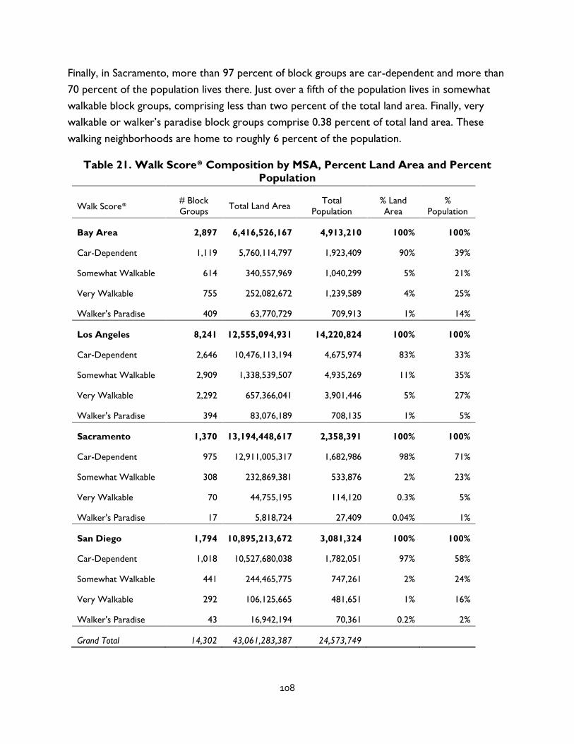
108
Finally, in Sacramento, more than 97 percent of block groups are car-dependent and more than
70 percent of the population lives there. Just over a fifth of the population lives in somewhat
walkable block groups, comprising less than two percent of the total land area. Finally, very
walkable or walker’s paradise block groups comprise 0.38 percent of total land area. These
walking neighborhoods are home to roughly 6 percent of the population.
Table 21. Walk Score® Composition by MSA, Percent Land Area and Percent Population
Walk Score® # Block
Groups Total Land Area
Total
Population
% Land
Area
%
Population
Bay Area 2,897 6,416,526,167 4,913,210 100% 100%
Car-Dependent 1,119 5,760,114,797 1,923,409 90% 39%
Somewhat Walkable 614 340,557,969 1,040,299 5% 21%
Very Walkable 755 252,082,672 1,239,589 4% 25%
Walker's Paradise 409 63,770,729 709,913 1% 14%
Los Angeles 8,241 12,555,094,931 14,220,824 100% 100%
Car-Dependent 2,646 10,476,113,194 4,675,974 83% 33%
Somewhat Walkable 2,909 1,338,539,507 4,935,269 11% 35%
Very Walkable 2,292 657,366,041 3,901,446 5% 27%
Walker's Paradise 394 83,076,189 708,135 1% 5%
Sacramento 1,370 13,194,448,617 2,358,391 100% 100%
Car-Dependent 975 12,911,005,317 1,682,986 98% 71%
Somewhat Walkable 308 232,869,381 533,876 2% 23%
Very Walkable 70 44,755,195 114,120 0.3% 5%
Walker's Paradise 17 5,818,724 27,409 0.04% 1%
San Diego 1,794 10,895,213,672 3,081,324 100% 100%
Car-Dependent 1,018 10,527,680,038 1,782,051 97% 58%
Somewhat Walkable 441 244,465,775 747,261 2% 24%
Very Walkable 292 106,125,665 481,651 1% 16%
Walker's Paradise 43 16,942,194 70,361 0.2% 2%
Grand Total 14,302 43,061,283,387 24,573,749

109
Note: the bars are ordered from darkest (car-dependent) to lightest (walker’s paradise)
Figure 32. Distribution of land use and population by Walk Score® categories and
by study region
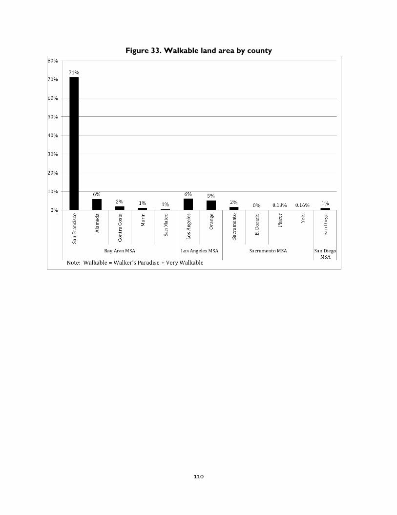
110
Figure 33. Walkable land area by county

111
Figure 34. Population in walkable areas by county
Neighborhood typology
Descriptions of the development of the neighborhood types are included in Blumenberg et al.
(2015) and Voulgaris et al. (forthcoming). They were constructed using data from three
sources, which were applied to census tracts across the U.S.: (1) data taken directly from the
Environmental Protection Agency (EPA) Smart Location Database, (2) data derived from the
EPA Smart Location Database, and (3) 2010 Decennial United States Census data. The variables
used in their factor analysis and their sources are summarized in Table 22. The five factors
created from the larger set of 20 variables generally indicate the degrees to which a
neighborhood is (1) dense, (2) diverse, (3) transient, (4) established, and (5) accessible.
The distribution of each factor among the census tracts throughout the United States is shown
in Figure 35. The distribution of the density variables across all census tracts is highly
asymmetric, since a small number of tracts are extremely dense, relative to most of the
country. Thus, the two factors that are most closely related to the density variables –density
and diversity– have distributions with very long tails.
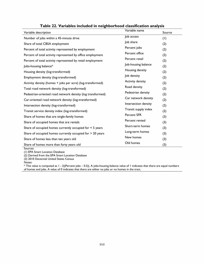
112
Table 22. Variables included in neighborhood classification analysis
Variable description Variable name
Source
Number of jobs within a 45-minute drive Job access
(1)
Share of total CBSA employment Job share
(2)
Percent of total activity represented by employment Percent jobs
(2)
Percent of total activity represented by office employment Percent office
(2)
Percent of total activity represented by retail employment Percent retail
(2)
Jobs-housing balance* Job-housing balance
(2)
Housing density (log-transformed) Housing density
(2)
Employment density (log-transformed) Job density
(2)
Activity density (homes + jobs per acre) (log-transformed) Activity density
(2)
Total road network density (log-transformed) Road density
(2)
Pedestrian-oriented road network density (log transformed) Pedestrian density
(2)
Car-oriented road network density (log-transformed) Car network density
(2)
Intersection density (log-transformed) Intersection density
(2)
Transit service density index (log-transformed) Transit supply index
(2)
Share of homes that are single-family homes Percent SFR
(3)
Share of occupied homes that are rentals Percent rented
(3)
Share of occupied homes currently occupied for < 5 years Short-term homes
(3)
Share of occupied homes currently occupied for > 20 years Long-term homes
(3)
Share of homes less than ten years old New homes
(3)
Share of homes more than forty years old Old homes
(3) Sources:
(1) EPA Smart Location Database
(2) Derived from the EPA Smart Location Database
(3) 2010 Decennial United States Census
Notes:
* This value is computed as 1 - 2|(Percent jobs – 0.5)|. A jobs-housing balance value of 1 indicates that there are equal numbers
of homes and jobs. A value of 0 indicates that there are either no jobs or no homes in the tract.

113
Figure 35. Distribution of factor scores between census tracts
The authors use standardized factor scores for each census tract to conduct the cluster analysis
and identify seven distinct neighborhood types: Rural, New development, Patchwork,
Established suburbs, Urban residential, Old urban, and Mixed-use.
Table 23 shows how the seven neighborhood types vary in terms of each of the
selected built environment characteristics.

114
Figure 36 shows how the factor scores vary among neighborhood types. The Patchwork and
Mixed-use neighborhood types, for example, have similar high scores on the jobs-housing
balance index; however, the housing density is much higher in Mixed-use neighborhoods than in
Patchwork neighborhoods. Likewise, the age of the housing in Old Urban neighborhoods is
similar to that in Established Suburbs, but the housing density in Old Urban neighborhoods is
nearly seven times that of Established Suburbs.
Table 23. Average built environment characteristics by neighborhood type
Homes
per acre
Jobs-
housing
balance
Percent
rental
homes
Percent of
homes > 40
years old
Jobs within a
45-minute
drive (in
thousands)
Transit
supply
index
All Neighborhoods 3.5 0.4 34% 46% 118 0.5
Rural 0.1 0.3 19% 42% 14 0.0
New development 1.4 0.2 19% 17% 68 0.0
Patchwork 1.7 0.7 35% 46% 94 0.1
Established suburbs 4.1 0.3 25% 74% 186 0.6
Residential urban 5.9 0.3 58% 56% 147 0.8
Old urban 27.5 0.3 76% 74% 533 4.2
Mixed-use 5.2 0.7 65% 49% 181 1.1

115
Figure 36. Variation in factor scores within and among neighborhood types

116
Figure 37. Characteristic images of each neighborhood type
Source: Google Earth, Google Maps
Although neighborhoods are not homogenous even within each type, Figure 37 illustrates each
neighborhood type in terms of a characteristic image. These images give an overall sense of the
qualitative differences among neighborhoods types. Map 4 illustrates the spatial arrangement of
the neighborhood types in Los Angeles.

117
Map 4. Example: Neighborhood types in the Los Angeles region
While all of the cities shown above have a cluster of Mixed-use neighborhoods at the city
center, this neighborhood type is not confined to downtowns. There are also mixed-use
neighborhoods in commercial centers located closer to the edges of each city. Likewise, there
are several Rural neighborhoods surrounded on all sides by Established Suburban
neighborhoods or even adjacent to Urban neighborhoods. Nevertheless, moving from the
center of each city to the outskirts, there is a distinct, if varied, progression from Mixed-use to
Old Urban to Urban Residential to Established Suburb to Patchwork to New Development to
Rural.
Figure 38 shows how the census tracts in each MSA in our study area are distributed among
the seven neighborhood types, and Figure 39 shows how walking mode shares differ by
neighborhood type.

118
Figure 38. Share of census tracts in each neighborhood type by MSA
Figure 39. Walking mode shares by neighborhood type
0%
10%
20%
30%
40%
50%
60%
70%
80%
90%
100%
Full Study
Area
Bay Area LosAngeles Sacramento San Diego
Job center
Old urban
Urban residential
Established suburb
Patchwork
New development
Rural
6% 4% 6% 7% 9% 17% 10%0%2%4%6%8%
10%12%14%16%18%20%
Walk
ing m
od
e s
hare
of
trip
s

119
Nodal degree
Average nodal degree is a measure of street connectivity. Nodal degree is the number of
streets that join at an average intersection. Average nodal degree is simply the average across
all intersections within a geographic area (such as a census tract). For example, Figure 40 shows
a simple street network with one four-legged intersection (nodal degree = 4), one three-legged
intersection (nodal degree =3), two two-legged intersections (nodal degree = 2), and three
dead ends (nodal degree = 1). The average nodal degree for this simple network would be the
average of the nodal degree for each individual intersection: (1 + 1 + 4 + 2 + 2 + 3 + 1) / 7
which is equal to two.
2
1
4
3
2 1
1
Figure 40. Illustration of nodal degree

120
Appendix D. Walk Score® by county
The following analysis considers Walk Score® across the 12 counties included in our study area.
San Francisco County has the lowest car-dependent land area, 17.73 percent, and the least
percentage of the population living there, 3.74 percent. The remaining 11 counties all have
more than 75 percent car-dependent land area. San Diego, Contra Costa, Marin, Sacramento,
El Dorado, Placer and Yolo Counties exceed 90 percent. El Dorado County leads with 99.77
percent; more than 93 percent of the county’s population resides there.
In Los Angeles County, nearly a third of residents live in car dependent, somewhat walkable, or
very walkable areas. Somewhat walkable areas surpass the other two categories just slightly
with 33.91 percent of the population, despite accounting for less than nine percent of the
county’s total land area. Orange County has the highest percentage of somewhat walkable land
area, 19.38 percent, and 37.60 percent of residents live there.
Only a few counties have more than 25 percent very walkable land areas. These include
Alameda, Los Angeles, San Francisco and San Mateo Counties.
Of the counties in our study, San Francisco County has the highest percentage of land area in
“walker’s paradise” neighborhoods, nearly 30 percent. The county with the second highest
percentage highly walkable neighborhoods is Alameda county where one percent of the land
area is located in “walker’s paradise.” Both of these counties fall within the Bay Area MSA
which explains why this region has the highest total land area and population that falls within
walkable neighborhoods. San Francisco differs from every other county by having more very
walkable or walker’s paradise land areas than somewhat walkable and car-dependent. In fact, 10
of the 12 counties analyzed have less than one percent walker’s paradise land area. Two
counties, El Dorado and Placer, have no walker’s paradise neighborhoods whatsoever.
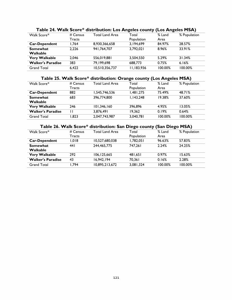
121
Table 24. Walk Score® distribution: Los Angeles county (Los Angeles MSA) Walk Score® # Census
Tracts
Total Land Area Total
Population
% Land
Area
% Population
Car-Dependent 1,764 8,930,366,658 3,194,699 84.97% 28.57%
Somewhat
Walkable
2,226 941,764,707 3,792,021 8.96% 33.91%
Very Walkable 2,046 556,019,881 3,504,550 5.29% 31.34%
Walker's Paradise 383 79,199,698 688,773 0.75% 6.16%
Grand Total 6,422 10,510,356,737 11,183,936 100.00% 100.00%
Table 25. Walk Score® distribution: Orange county (Los Angeles MSA) Walk Score® # Census
Tracts
Total Land Area Total
Population
% Land
Area
% Population
Car-Dependent 882 1,545,746,536 1,481,275 75.49% 48.71%
Somewhat
Walkable
683 396,774,800 1,143,248 19.38% 37.60%
Very Walkable 246 101,346,160 396,896 4.95% 13.05%
Walker's Paradise 11 3,876,491 19,362 0.19% 0.64%
Grand Total 1,823 2,047,743,987 3,040,781 100.00% 100.00%
Table 26. Walk Score® distribution: San Diego county (San Diego MSA) Walk Score® # Census
Tracts
Total Land Area Total
Population
% Land
Area
% Population
Car-Dependent 1,018 10,527,680,038 1,782,051 96.63% 57.83%
Somewhat
Walkable
441 244,465,775 747,261 2.24% 24.25%
Very Walkable 292 106,125,665 481,651 0.97% 15.63%
Walker's Paradise 43 16,942,194 70,361 0.16% 2.28%
Grand Total 1,794 10,895,213,672 3,081,324 100.00% 100.00%

122
Table 27. Walk Score® distribution: San Francisco county (Bay Area MSA) Walk Score® # Census
Tracts
Total Land Area Total
Population
% Land
Area
% Population
Car-Dependent 17 21,459,825 36,602 17.73% 3.74%
Somewhat
Walkable
49 13,474,656 79,707 11.13% 8.15%
Very Walkable 215 50,310,166 341,174 41.57% 34.87%
Walker's Paradise 298 35,786,228 521,068 29.57% 53.25%
Grand Total 579 121,030,875 978,551 100.00% 100.00%
Table 28. Walk Score® distribution: Alameda county (Bay Area MSA) Walk Score® # Census
Tracts
Total Land Area Total
Population
% Land
Area
% Population
Car-Dependent 359 1,669,020,681 630,104 87.20% 35.25%
Somewhat
Walkable
274 131,038,588 465,061 6.85% 26.02%
Very Walkable 324 94,852,538 536,186 4.96% 30.00%
Walker's Paradise 89 19,133,207 156,214 1.00% 8.74%
Grand Total 1,046 1,914,045,014 1,787,565 100% 100%
Table 29. Walk Score® distribution: Contra Costa county (Bay Area MSA) Walk Score® # Census
Tracts
Total Land Area Total
Population
% Land
Area
% Population
Car-Dependent 434 1,754,125,281 732,430 93.71% 68.67%
Somewhat
Walkable
125 80,932,814 206,591 4.32% 19.37%
Very Walkable 73 35,249,102 121,774 1.88% 11.42%
Walker's Paradise 4 1,586,764 5,805 0.08% 0.54%
Unmarked 1 - - 0.00% 0.00%
Grand Total 637 1,871,893,961 1,066,600 100% 100%
Table 30. Walk Score® distribution: Marin county (Bay Area MSA) Walk Score® # Census
Tracts
Total Land Area Total
Population
% Land
Area
% Population
Car-Dependent 117 1,307,922,725 200,813 97.02% 69.14%
Somewhat
Walkable
34 23,737,101 54,585 1.76% 18.79%
Very Walkable 21 15,570,108 31,155 1.16% 10.73%
Walker's Paradise 2 811,412 3,893 0.06% 1.34%
Grand Total 174 1,348,041,346 290,446 100% 100%
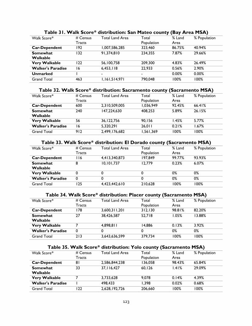
123
Table 31. Walk Score® distribution: San Mateo county (Bay Area MSA) Walk Score® # Census
Tracts
Total Land Area Total
Population
% Land
Area
% Population
Car-Dependent 192 1,007,586,285 323,460 86.75% 40.94%
Somewhat
Walkable
132 91,374,810 234,355 7.87% 29.66%
Very Walkable 122 56,100,758 209,300 4.83% 26.49%
Walker's Paradise 16 6,453,118 22,933 0.56% 2.90%
Unmarked 1 - - 0.00% 0.00%
Grand Total 463 1,161,514,971 790,048 100% 100%
Table 32. Walk Score® distribution: Sacramento county (Sacramento MSA) Walk Score® # Census
Tracts
Total Land Area Total
Population
% Land
Area
% Population
Car-Dependent 600 2,310,509,005 1,036,949 92.45% 66.41%
Somewhat
Walkable
240 147,224,630 408,253 5.89% 26.15%
Very Walkable 56 36,122,756 90,156 1.45% 5.77%
Walker's Paradise 16 5,320,291 26,011 0.21% 1.67%
Grand Total 912 2,499,176,682 1,561,369 100% 100%
Table 33. Walk Score® distribution: El Dorado county (Sacramento MSA) Walk Score® # Census
Tracts
Total Land Area Total
Population
% Land
Area
% Population
Car-Dependent 116 4,413,340,873 197,849 99.77% 93.93%
Somewhat
Walkable
8 10,101,737 12,779 0.23% 6.07%
Very Walkable 0 0 0 0% 0%
Walker's Paradise 0 0 0 0% 0%
Grand Total 125 4,423,442,610 210,628 100% 100%
Table 34. Walk Score® distribution: Placer county (Sacramento MSA) Walk Score® # Census
Tracts
Total Land Area Total
Population
% Land
Area
% Population
Car-Dependent 178 3,600,311,201 312,130 98.81% 82.20%
Somewhat
Walkable
27 38,426,587 52,718 1.05% 13.88%
Very Walkable 7 4,898,811 14,886 0.13% 3.92%
Walker's Paradise 0 0 0 0% 0%
Grand Total 213 3,643,636,599 379,734 100% 100%
Table 35. Walk Score® distribution: Yolo county (Sacramento MSA) Walk Score® # Census
Tracts
Total Land Area Total
Population
% Land
Area
% Population
Car-Dependent 81 2,586,844,238 136,058 98.43% 65.84%
Somewhat
Walkable
33 37,116,427 60,126 1.41% 29.09%
Very Walkable 7 3,733,628 9,078 0.14% 4.39%
Walker's Paradise 1 498,433 1,398 0.02% 0.68%
Grand Total 122 2,628,192,726 206,660 100% 100%

124
Appendix E. Walk Score® by metropolitan region
Map 5. Bay Area Walk Score®
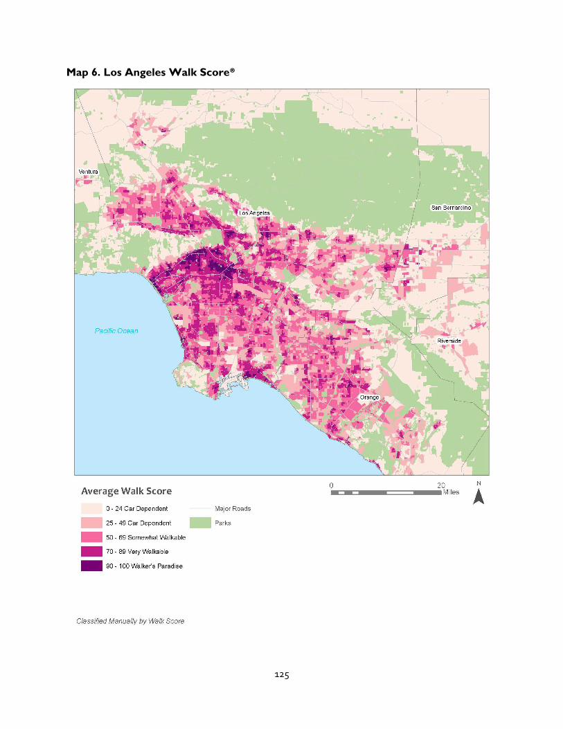
125
Map 6. Los Angeles Walk Score®

126
Map 7. Sacramento Walk Score®

127
Map 8. San Diego Walk Score®

128
Appendix F. Interview protocol
1. Walk me through how your agency completes your regional travel modeling.
a. Where do you get the data about the trips?
b. What modes are included?
2. Are the inputs or outputs validated? If so, how?
3. What is the purpose of conducting these regional travel demand models?
4. What are the implications of these modeling efforts, after they are calculated, how are they
used by your agency?
5. To what extent do other agencies in the region make use of these results?
6. What changes, if any, have been made to your modeling approach in the last ten years or
so?
7. How often do you inventory regional land use/built environment changes that may have an
effect on travel? How are these land use changes incorporated into the travel demand
modelling process?
8. How does your modeling process account for short trips and/or trips that begin and end
within the same traffic analysis zone?
9. Thinking about different types of trips in terms of length, purpose, and mode, which types of trips do you believe the model is best able to predict, and which types do you believe it is
least able to predict? At what point might this type of bias become a problem? How might
you correct for this kind of bias if it were to become a problem?
10. How does the model account for multi-modal trips, for example those in which someone
walks, bikes, or drives to a transit stop or station, or walks from a remote parking space to
their final destination?
11. Based on your own personal judgment, what is your best guess for the proportion of
unlinked trips in your region are walk trips? What about transit trips?