hedonic analysis of housing prices near the portland urban
TRANSCRIPT

Portland State UniversityPDXScholar
Dissertations and Theses Dissertations and Theses
1996
Hedonic Analysis of Housing Prices Near the Portland UrbanGrowth Boundary, 1978-1990Abdullah AlkadiPortland State University
Let us know how access to this document benefits you.Follow this and additional works at: http://pdxscholar.library.pdx.edu/open_access_etds
This Dissertation is brought to you for free and open access. It has been accepted for inclusion in Dissertations and Theses by an authorizedadministrator of PDXScholar. For more information, please contact [email protected].
Recommended CitationAlkadi, Abdullah, "Hedonic Analysis of Housing Prices Near the Portland Urban Growth Boundary, 1978-1990" (1996). Dissertationsand Theses. Paper 1345.
10.15760/etd.1344

HEDONIC ANALYSIS OF HOUSING PRICES NEAR THE
PORTLAND URBAN GROWTH BOUNDARY, 1978-1990
BY
ABDULLAH ALKADI
A dissertation submitted in partial fulfillment of the requirements for the degree of
DOCTOR OF PHILOSOPHY in
URBAN STUDIES
Portland State University
© 1996
-----------------·

DISSERTATION APPROVAL
The abstract and dissertation of Abdullah Alkadi for the Doctor of Philosophy in
Urban Studies was presented May 6, 1996 and accepted by the dissertation
committee and the doctoral program.
APPROVALS:
, James G. Strathman
Deborah Howe
Thomas Harvey, Representative of the Office of Graduate Studies
* * * * * * * * * * ** ** * * * * * ................ "' ............................ :l<.:!<.i<.:i<.*-"-*.:!L**-*-*-*~*---*-*-*** * * ** * * * * * * * * *
ACCEPTED FOR PORTLAND STATE UNIVERSITY LIBRARY
by

ABSTRACT
An abstract of the dissertation of Abdullah Alkadi for the Doctor of
Philosophy in Urban Studies presented May 6, 1996.
Title: Hedonic Analysis of Housing Prices near the Portland Urban
Growth Boundary, 1978-1990.
The cornerstones of Oregon's 1973 Senate Bill 100 are the
preservation of farm, forest, and other resource lands and the
containment of urban development within urban growth boundaries
(UGB). The UGB is a boundary around each incorporated city
containing enough land to meet projected needs until the year 2000.
The Land Conservation and Development Commission
(LCDC), charged with adopting and implementing state planning
policy, sought to keep UGBs small enough to contain urban sprawl.
To avoid the potential effects of land price inflation, LCOC allowed
UGBs to include more land supply than the forecasted demand. The
Portland-Metropolitan region was allowed to have a 15.3-percent
surplus.
Policy makers are unsure what effect UGBs have on housing
costs. The common belief is that by restricting the amount of land
available for residential construction the market drives prices up.
Contrasting opinions suggest that by substituting low-density with
high-density development, per-unit construction costs are lower, thus
reducing the costs of owning a hom.e_. -------··.
Efforts to dispel some of the mystery about the relationship
between UGBs and housing prices are needed. The objective of this

research is to provide empirical evidence of the relationship between
the Portland-Metropolitan area's UGB and housing prices. The study
uses a hedonic model to conduct a time-series analysis for the years
1978 to 1990 for Washington County.
This study found no relationship between housing price and
the imposition of the UGB. In fact, the rate of increase in price for
single-family housing after UGB implementation was found to be
much less than before. Proximity as measured by distance of sale to
the UGB was the only variable that was associated with a higher rate
of increase in housing prices.
All of these results, with the exception of those related to
proximity, were unexpected but may be explained by several factors:
imposition of the Metropolitan Housing Rule in 1981, a severe
recession during the 1980s, and excess land supply. These influences
do not support a conclusion that UGBs lead to an increase in housing
prices, at least prior to 1990, when the UGB did not constrain the
supply of land.
------------------·

The Opening
In the name of God, the Compassionate, the Merciful
All praise belongs to God, Lord of all world,
the Compassionate, the Merciful,
Ruler of Judgment Day.
It is You that we worship, and to You we appeal for help.
Show us the straight way,
the way of those You have graced, not of those on whom is Your wrath, not of those who wander astray.
The Arabic text is the first Surat (chapter) of the Holy Qur-an and the English is the translation of the meaning by 1l1omas Cleary ·from his book The Essential Koran.
---- -· ··--------··.

rtliis (])issertation Is (])ecficatecf rto
rrrie memory of my 6e(oved fatfzer, Hussain wfzo was tfze force 6efzind my education. :May }l.((afz sfzower J{is :Mercy on fzim and grant fzim paradise
:My motfzer, :Noorafi, wfzo nurtured me
:My wife for fzer (ove and devotion
:My cfzz'fdren, :Noorafz, }1.6rar, 1vtofzammec£; and :Man'am for their patience and support
:My 6rotfzers and sisters, for tfzeir encouragement
and
:My friends 1vfzo inspired confidence in me
-----· -· ··--------··
·-------·- ------

ACKNOWLEDGMENTS
Praise Be to Allah For His Bounty and Mercy that I have
completed this study.
I am most indebted to Dr. Nohad Toulan who guided me and
provided me with unstinting support, especially during the critical
early stages of my research plan by helping me to conceptualize the
dissertation focus.
My deep gratitude to Dr. James Strathman, my academic
advisor. I wish to express my appreciation for the time and energy he
has invested in ensuring the successful completion of my research.
No amount of words can adequately convey my heartfelt thanks for
his encouragement that saw no bounds.
Additionally, my sincere thanks to Dr. Kenneth Dueker, Dr.
Deborah Howe, and Dr. Thomas Harvey who comprised my
Dissertation Committee.
I am intellectually indebted to Portland State University
especially the School of Urban and Public Affairs for the quality of
instruction that I have been fortunate to experience. Equally, I am
appreciative for the financial support provided by King Faisal
University for my graduate studies.
My deepest gratitude to the Honorable Mr. Sa'ad Al-Othman,
Deputy Governor of the Eastern Province of the Kingdom of Saudi
Arabia, whose personal interest and enthusiasm for my work
encouraged me to pursue my educational goals. Also my thanks to
Mr. Faisal Al-Othman, Director of the office of the Deputy Governor.
I would like to also thank the staff of the Department of Land
Use and Transportation and the Department of Assessment and

Taxation at Was.litington County for assisting me with the necessary
data to complete my research.
Finally, I thank Dr. Martha Bianco and Mr. Mohammad
McCabe for ~heir assistance in editing the dissertation.
------·-------------·

TABLE OF CONTENTS
CHAPTER PAGE
I. INTRODUCTION................................................................................ 1
Research Objectives................................................................... 4
Historical Background............................................................... 6
Organization of the Study ....................................................... 9
II. LITERATURE REVIEW................................................................... 11
Theoretical Foundation of the Housing Market............... 11
1. Housing Prices from the Supply-Demand
Framework....................................................................... 12
a. Supply-Side Factors............................................ 12
b. Demand-Side Factors......................................... 15
2. Land Use and Housing Price Theories................... 17
a. Accessibility Factors........................................... 19
b. Public Service Factors........................................ 23
c. Structure and Site Factors................................. 26
d. Neighborhood Factors...................................... 27
Empirical Studies of Land Use Controls and Housing
Prices........................................................................................... 29
Concluding Remarks............................................................... 46

CHAPTER
TABLE OF CONTENTS (CONTINUED)
I
ii
PAGE
III. RESEARCH METHODOLOGY ....................................................... 48
Statement of the Problem....................................................... 48
Factors Contributing to Housing Prices............................... 49
Research Hypotheses............................................................... 51
Models for Examining the Relationship between
UGBs and Housing Prices....................................................... 52
Conceptual and Operational Model..................................... 56
Variable Measurement and Data Sources........................... 62
IV. DATA ANALYSIS AND RESEARCH FINDINGS ................... 69
Data Analysis............................................................................. 69
Model Refinement................................................................... 71
Research Findings.................................................................... 73
UGBs and Rate of Increase in Housing Prices.................... 73
Rate of Increase in Housing Prices in the Latter Periods 81
Rate of Price Increases of Single-Family Houses on
Larger Lots.................................................................................. 88
Sun1mary................................................................................... 91
-----· -· ··--------··

iii
TABLE OF CONTENTS (CONTINUED)
CHAPTER PAGE
V. CONCLUSIONS AND POLICY IMPLICATIONS ...................... 92
Major Findings......................................................................... 92
Research Limitations............................................................... 96
Generalization of the Study................................................... 98
Policy Implication and Future Research............................. 99
SELECTED BIBLIOGRAPHY......................................................... 103
iv
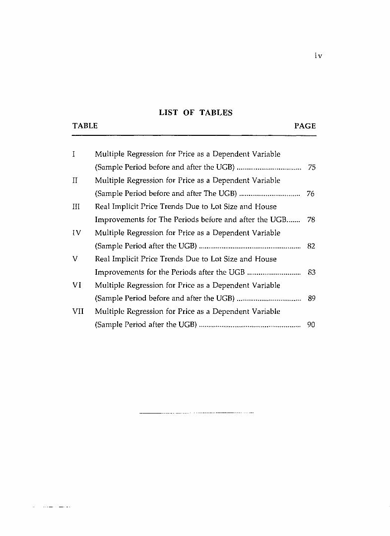
LIST OF TABLES
TABLE PAGE
I Multiple Regression for Price as a Dependent Variable
(Sample Period before and after the UGB) .................................. 75
II Multiple Regression for Price as a Dependent Variable
(Sample Period before and after The UGB) ................................ 76
III Real Implicit Price Trends Due to Lot Size and House
Improvements for The Periods before and after the UGB....... 78
IV Multiple Regression for Price as a Dependent Variable
(Sample Period after the UGB) ...................................................... 82
V Real Implicit Price Trends Due to Lot Size and House
Improvements for the Periods after the UGB ............................ 83
VI Multiple Regression for Price as a Dependent Variable
(Sample Period before and after the UGB) .................................. 89
VII Multiple Regression for Price as a Dependent Variable
(Sample Period after the UGB) ...................................................... 90

v
I~IST OF FIGURES
FIGURE PAGE
1 Population Trends for the Portland Metropolitan Area and
Washington County forthe Period 1970-1990.............................. 7
2 Employment Trenc:!s for the Portland Metropolitan Area
for the Period 1979-1990J............ ...... ....... .... ... .............. .... ..... ........ ..... 8
3 Single-Family Home Prices for the Portland Metropolitan
Area, 1979-1990 ............... : ..................................................................... 9
4 Factors Theoretically Influencing Residential Land Price
Variations ................. ,.......................................................................... 18
5 UGB and Supply RE~striction Effects.............................................. 31
6 Bid-Rent Function "nd Itiousehold Size...................................... 39
7 Bid-Rent Function •md Household Size after the UGB is
Imposed................................................................................................ 40
8 Changes in Deman~:! foriLand as Time Passes while Land
Supply is Constrained by the Imposition of the UGB............... 57
9 Washington County Map with the Urban Growth
Boundary.............................................................................................. 65
10 Average Price for S~nglei-Family Dwellings sold, 1978-1990.... 70
11 Average Lot Size for Single-Family Dwellings sold,
1978-1990 .................. , ........ , ................................................................... 71
12 Average Interior Square; Footage for Single-Family
Dwellings sold, 1978:1~90 ...... :·.:~==:·:.-:-:-:-:-.-:.:~: .. ~ .. -:-:......................... 72

LIST OF FIGURES (CONTINUED)
FIGURE
13 Real Implicit Price Trends per Month Due to Lot Size and
House Improvements for the Periods before and after
vi
PAGE
the UGB ............................................................................................... 79
14 Real Implicit Price Trends per Month Due to Lot Size and
House Improvements for the Four Subperiods After the
UGB ............................ : ......................................................................... 84
15 Changes in Building Permits Issued Between 1980 and 1990.. 86
-----· -· ··---------··.

CHAPTER I
INTRODUCTION
1
The United States post-World War II population growth has
significantly shifted away from the central cities, with the automobile,
federal highway programs, and federal housing policies lessening the
individual's reliance on the central city. The rate of population
growth in the suburbs, compared to population growth in the central
cities, has been extraordinary. Populations in the 1950s and 1960s in
the suburbs surrounding the nation's largest metropolitan areas grew
by 53.9 percent while the central cities added only 1.5 percent to their
population. Between 1960 and 1985, the population increase in the
United States was estimated to be 73 million persons with almost 80
percent of this growth (58 million persons) estimated to live in
suburban communities. Furthermore, the total suburban population
rose from 41 million in 1950 to 115 million in 1990, an increase of 181
percent compared with a 65 percent increase in total population
(Downs 1994).
The substantial increase in the areas surrounding central cities
has resulted in a sprawling pattern of urban development with huge
amounts of rural/farm land being transformed to accommodate this
urban expansion. Rural landscapes, which once were dominated by
agricultural uses, have been converted into housing, shopping
centers, roads, industrial facilities and office spaces. Urban sprawl has
consumed land at a much faster rate than the population (Toulan
1965), an example being that during the l26_Qs, totaLurban population
increased by 21 percent while the consumption of land for urban uses
increased by 36 percent (Nelson 1984).

2
The state of Oregon has not been immune to this migration
from urban areas to the rural environs. The state has been a popular
destination for people from other states, which has exacerbated urban
sprawl and resulted in the loss of open space. In the 1960s, the ability
of Oregon's fiscal base and environment to manage the sprawling
development started to become a growing concern among lawmakers,
with the provision of sewer, water and other necessary infrastructure
services to the low-density suburban developments generating
additional costs that the state's natives were reluctant to pay. The
result was a strained relationship between long-time residents and
new arrivals, who received much of the blame for the perceived ills of
rapid urban development. This anti-growth sentiment was voiced by
then-Governor Tom McCall and his not-so subtle greetings at the
California border pleading for visitors to "enjoy your visit, but don't
stay."
Environmental concerns focused on the diminishing amount
of forest and agricultural land, the backbone of the state's economy,
with the greatest loss occurring in the fertile Willamette Valley, which
stretches south from Portland for approximately 100 miles. The
Willamette Valley accounts for only a small percentage of the state's
land area, yet it is home to nearly 75 percent of the state's population
(Howe 1993). There was a widespread fear that the tide of urban
development would eventually wash over the Willamette Valley if
the state did not take strong measures to guide, direct, and control the
quality of this growth (DeGrave 1984).
Despite the anti-growth atmosphere in the state, its legislators
acknowledged the reality of thP growth and were prepared to confront
the issue with the result that in 1969, the Oregon legislature passed
Senate Bill 10, an initiative which required all cities and counties to

3
adopt and apply comprehensive planning and zoning ordinances
addressing nine statewide goals, including growth management
(Toulan 1994; Knaap & Nelson 1992 ). The plans were to be reviewed
and approved by the Governor. This first attempt at legislatively
controlling development failed, as there was insufficient staff to push
local governments and no penalties for noncompliance (Nelson 1992).
In 1973 the legislature tried again, passing Senate Bill 100. The
cornerstones of this initiative were the preservation of farm, forest,
and other open space or environmentally sensitive land and the
containment of urban development within urban growth boundaries
(Nelson 1992). The urban growth boundary (UGB) was to be
established around each city or urbanized area, containing enough
land to meet projected development needs until the year 2000. All
land in the state was to be either inside UGBs or classified for
exclusive resource uses. With some exceptions, for example large
acreage lots, residential development outside UGBs was to be stopped.
Land within the boundary, even undeveloped and agricultural land,
was available for conversion into urban use.
Determining how much land was to be included within UGBs
was often controversial. Localities fought to include enough land in
order to avoid land price inflation. The commission that was created
with Senate Bill 100, the Land Conservation and Development
Commission (LCDC), was charged with adopting and implementing
state planning policy and sought to keep UGBs small enough to
contain urban sprawl (Knaap & Nelson 1992). However, to avoid the
potential effects of land price inflation, the LCDC made sure that UGBs
contained more land than forecasted for the year 2000; for example,
the Portland metropolitan region was allowed to have a 15.3 percent
land surplus (Nelson 1994).

4
Even if UGBs contain more than enough land for future
development, policy makers are unsure what effect these boundaries
have on housing costs. The common belief is that by restricting the
amount of land available for residential construction the market
would drive prices up. Contrasting opinions suggest that by
substituting low-density development with high density, costs
associated with the provision of public services would be reduced,
thus lowering the cost of owning a horne (Abbott, Howe, Adler 1994).
Efforts to dispel some of the mystery about the relationship
between UGBs and housing prices are needed. The objective of this
research is to conduct a hedonic analysis of detached single family
housing prices near the Portland metropolitan area's UGB.
RESEARCH OBJECTIVES
The primary objective of this research is to examine changes in
the detached single-housing prices that occurred shortly after the
implementation of the Portland metropolitan area's UGB. There are
many factors that can influence the housing market. This study
attempts to examine the relationship of UGBs and housing price,
while holding other important variables affecting price constant.
These other variables include factors such as interest rates,
accessibility, housing site and structure, and neighborhood
characteristics. To examine the changes in the detached single
housing prices, this research utilizes hedonic analysis, which simply
measures a relationship between housing unit attributes and market
prices.
The examination of the changes in the detached single-housing
prices that are concurrent with UGBs has several implications for
policy makers. A better understanding of the behavior of the housing

5
market concurrent with UGBs would help planners and public
officials in analyzing the desirability of adopting such a program for a
particular community. In addition, this research should help policy
makers develop an economic rationale for the need for extending
UGBs to other areas designated as non-urban. Finally, the study
should enrich the growth management literature as it will dispel
some of the ambiguities about changes in the market for single-family
houses associated with UGBs.
This study is focusing only on the market for the detached
single-family horne for two main reasons. First, the rental market is
different from the ownership market. Second, UGBs are imposed to
control urban sprawl and low densities, which are fueled by single
family housing.
The Portland metropolitan area's UGB was implemented in
October 1980. As a result this study examines the changes in the
detached single-family housing market for a few years before (back to
January 1978) and a few years after (up to 1990, the midpoint of the
UGB's designated period).
The Portland area was chosen because it is one of the fastest
growing areas in the U.S., and the UGB has been in place long enough
for any changes in the housing market to become apparent. However,
the Portland area is too large an area to be examined; therefore,
Washington County was chosen from the Portland area. This
research is focusing on Washington County because it is the fastest
growing of the three counties, Multnomah, Clackamas, and
Washington. In addition, the data for Washington County is
cornpu terized and w'-"--""e'"'ll'--'e.__.s~t=ab=l._..is___.hc"e.._.d.._.. ______ _
The Portland area in general and Washington County in
particular have a history of rapid growth in population and

6
employment during the last few decades. A brief historica.l
background about some trends should help the reader to understand
the forces behind the dynamics of the housing market.
HISTORICAL BACKGROUND
The purpose of this section is to give a brief discussion about
population, employment, and housing trends for Washington County
and the Portland metropolitan area. Portland is, comparatively
speaking, a young city. Portland was incorporated only 150 years ago.
In 1860 the population did not exceed 2,844 people. The increase in
railroad connections, streetcar lines, paved roads and electric lights,
made the area start to grow significantly after the turn of the century.
As a result of World War II, the metropolitan area population grew
from about 500,000 in 1940 to over 660,000 in 1944 (Abbott 1983;
Friedman 1993).
In 1950, the Portland region was horne to 620,000 people. ThE.~
area kept increasing at a rapid pace to 822,000 in 1960 and 1,007,130 in
1970. This increase was fueled by the immigration of many
Californians who moved north to escape smog, traffic, crowds,
earthquakes, crime, the drought, and economic woes.
After 1970 the region's population grew at an even faster rate ..
As shown in Figure 1, from 1970 to 1990 the population of th~~
Portland metropolitan area increased from 1,007,130 to 1,495,548-·
almost 50 percent. Washington County's population increased from
157,920 to 311,554- almost 98 percent.
This increase in population :-va~sso_~l~t_ed wi_th a growth in th(t
regional economy. As shown in Figure 2, the total employment of th(t
Portland metropolitan area increased from 518,200 in 1979 to 636,900
in 1990-an increase of over 22 percent. However, employment i fl.

7
Washington County had a greater expansion. The total employment
went from 33,324 in 1960 to 172,008 in 1990- an increase of 416
percent.
POPULATION TRENDS
1,ffl0,000 ...------------------------. 1,400,000
1,200,000
~ 1,000,000
5 000,000 I.LI c.. roo,ooo
400,000
200,000
0
1970 1975 1980 1985
YEAR
1988 1989 1990
lcrmTLAND METRO AREA Iii WASHINGTON COUNTY I
Figure 1. Population Trends for the Portland Metropolitan
Area and Washington County for the Period 1970-1990. Source:
RMLS 1990.
The region's economy was hit by a very severe recession in
early 1980s, but it rapidly regained its strength as employment went up
by 28,800 (5.2 percent) in 1988, 31,200 (5.4 percent) in 1989, and 22,500
(3.71 percent) in 1990.
The median family income for the Portland area increased
throughout the 1960-1990 period. The median family income for
Washington County was even higher than in the metro area. The
difference between the two adjacent areas peaked in 1990, when

8
Washington County enjoyed a median income in the $40,000-$45,000
range versus a metropolitan area median of just over $30,000.
F-< z w -~ :;... 0 ..1 ~
:E w ..1 < F-< 0 F-<
EMPLOYMENT TRENDS
700,000
600,000 ~ r:;:
i~ 1'\7 '1:~
~ :{_z ~i 500,000 ~ ':"" m; 7; '-::' f;.~ ~~ z·.: r;": ~ <:.\·. ':1 ::.,i-., J ~-~\ ';'1-. '\ ~
~.4 \ '.f.~ ·.~) ,.
~1 ~~X: ·.·t ' . ' ·'· iH
400,000 ),• ~- ;~ ;I;.~ -it -~ nt ... :'i f~: ~(·;~~. t·': ,_ ;;.> ... '<l'A "" .): .:,i . ,. ... #
$ f)]' :t ;: ' •• <{ ',~: .,l 300,000 ~ ,., ... ~~> :..t·
',f·, .. , . :f ·:= ; ~" "!o~' Lh .,
' \'!; .. "'~ :T ;:~~ ·"'~ ·:,~:... ., .~ ~ '_f ·~ "i ~·~
~1; ;.~; ~~~, 200,000 ·~H
:~ . ~~ ,.,, . ~s: :if:j ,,;.:,
'~ ~:f \""J' .,....,_
~ ··.• ~~ ~~ ::~ . ,;_, ~'.;' ~; ~j h"" .
100,000 •;;· _.·~ ~:: ~-~ ~' r~:
~i :.'t: "· fJ ... ~: '""· t~ ~-~ ;:; "' /'j ';2 It,..~ ·~~ .:;-{ f~ ·i~ /{ .;_ .. ~}~ ·~'(· f$~ ;'3.
0 !J· *'"
.:-<; .1)
1979 1980 1981 1982 1983 1984 1985 1986 1987 1988 1989 1990
YEAR
loTOTAL EMPLOYMENT I
Figure 2. Employment Trends for Portland Metropolitan Area
for the Period 1979-1990. Source: RMLS 1991
Growth in population and economic prosperity led to a strong
regional housing market and a concomitant rise in housing prices.
Single-family housing permits for the four-county area (Multnomah,
Washington, Clackamas, and Clark County) went up from 5,756 in
1980 to 8,315 in 1990- an increase of 45 percent. As shown in Figure
3, the average housing value in 1979 was $65,500 for the metropolitan
area, while the median sales price was $59,900. These figures went up
to $96,000 for the average housing value in 1990, while the median
sales price was $79,700. The same figure shows a decline in the
average housing values during 1982, 1983, 1984, and 1985. This decline

9
was a natural reflection of the recession in the economy that took
place in early 1980s.
(JJ
u 0:: Q..
$100,000 $90,000 $80,000 $70,000 $60,000 . $50,000 . $40,000 $30,000 $20,000 $10,000
$0
HOUSING PRICES TRENDS
~ •,;
~ ~
~ r::
17 I"' r;; c ~ 'it ~ ~t r;: ·. ~~ r~ ·,, ' ~~ ,:;. (i~: q ~ '
,. " ~
}-\ f~ ., :-;,,' :~
,;.
' .,o;
~~ ~~ .
t :\ ·.~ :1 r:: j ¥ .\ " .{~ •) ;< ~
·; \ · .. ~: ~ ~ ;\ ;)) ·:~
·~ •. ~ }
;~~ -~ ~
'L4.
" .t: li .;, .... ·~; ;;: .. ;•,
11· •' ~A 7( ~ tt ~·
.~ ;i ,;~ ),;,
'* ;I :I 1:: il ,1;1 11 ~. ~- ~a " ,:. ;:1m I.: ~a "' (;• " II ·' ~ il ~· ,!.
-~ "' I
1979 1980 1981 1982 1983 1984 1985 1986 1987 1988 1989 1990
YEAR
lcAVERAGESELLINGPRICE IISALES I
Figure 3. Single-Family Home Prices for the Portland
Metropolitan Area, 1979-1990. Source: RMLS 1990.
ORGANIZATION OF THE STUDY
This study is organized into five chapters. Chapter I, the
introduction, discusses the general scope of the problem, the study
objective, the historical background of the area of study, and the study
outline. Chapter II gives a brief review of related literature in two
sections.
The first sectiuiL LOH::;bt:; ·of i:wo·--patts which review the
dynamics of the housing market. Part one spells out most of the
factors that affect the supply-demand framework. Part two discusses

10
land use and housing price theories. This second part deals mainly
with factors that affect housing prices from a spatial point of view.
The second secti011 reviews empirical studies that address
variables which affect housing prices. This section focuses mostly on
studies dealing with housing prices and land use controls. Sections
one and two pave the way for this research to develop a model that -·
could be used to test the relationship between UGBs and housing
prices.
Chapter II concludes with a brief summary of empirical studies
about urban growth controls and housing prices. Chapter III discusses
the methodology used for this research in terms of the necessary
approaches to problem examination and research design.
Chapter IV presents the empirical analysis of the research
questions. In particular, it analyses the data of the study, it discusses
the research findings, and then it gives a brief summary of the main
analysis in this chapter. Chapter V presents the major research
findings and concludes with policy implications and some suggestions
for future research.

CHAPTER II
LITERATURE REVIEW
11
The purpose of this chapter is to present a theoretical
perspective on the relationship between land use controls and
housing prices. There have been various studies of housing prices
and land use controls. In order to establish the connection between
housing prices and UGBs, it is necessary to explore the findings of
these studies to identify relevant variables.
The exploration is in two sections with the first providing a
theoretical foundation of the housing market by examining the
supply-demand framework and then land use and housing price
theories. The second section analyzes the empirical studies which
integrate land use controls and housing prices. This is followed with a
conclusion.
THEORETICAL FOUNDATION OF THE HOUSING MARKET
The housing market is fairly complex with numerous variables
playing significant roles in determining its behavior. Many
participants contribute to the housing market, including land
developers, builders, Realtors, financial institutions, and local
governments; these participants provide the inputs necessary for
housing development (Knaap and Nelson 1992). Another part of the
housing market equation is housing characteristics, including the
quality of the dwelling itself, the size of the dwelling, and site
characteristics (Kain and Quigley 1970). Each single house and the lot

12
on which it is located is unique in terms of size, location, topography,
subsoil conditions, public regulations, supporting services, ownership,
and future utility. Housing prices vary with these attributes and with
the conditions of sale (Black and Hoben 1985).
Given this complexity, this research utilizes economic theories,
such as the supply-demand framework and the bid-rent function, in
determining the factors that affect the housing market. Recognizing
the multiplicity of participants in the housing market, the following
discussion analyzes the housing market from two perspectives. The
first employs the supply-demand framework and the second a land
use approach.
1. Housing Prices from the Supply-Demand Framework
Supply-demand functions determine the basis for the housing
market with the supply function being represented by the standing
stock in the housing market, while the demand function is
represented by the consumers' desire and ability to have a certain type
of housing. This interaction of supply and demand factors determines
housing prices (Black and Hoben 1985; Manchester 1987). However,
there are factors that influence each side of the supply-demand
framework and the following is an analysis of the supply-demand
framework and the variables that could influence each side.
a. Supply-Side Factors
On the supply side, the cost of housing inputs (land, labor,
capital, and materials) could affect the quantity supplied. Regulatory
restrictions, restrictjo~g_n ___ service facilities (infrastructure), natural
restrictions, environmental restrictions, ownership characteristics and
tax policy could exacerbate the cost of housing inputs (Black and

13
Hoben 1985; Deakin 1991). In fact, land use controls influence the
housing market primarily through the market for land, an example
being that a parcel of laitd cannot be used for housing construction
until the parcel has been zoned by local governments for residential
use (Landis 1986; Niebanck 1991; Lowry and Ferguson 1992; Knaap and
Nelson 1992; Downs 1994).
In some cases, local governments zone enough land for
residential use, but restrict the supply of residential units by placing an
annual cap on housing permits. This type of limitation on the
residential supply causes housing prices to rise. Schwartz, Hansen,
and Green (1984) conducted a study on Petaluma, California, after it
placed an annual cap on building permits of a maximum of 500
permits per year, well below recent and expected demand. Their study
found that Petaluma's housing prices were 9 percent higher than
similar units in nearby Santa Rosa, California, where a limitation on
housing supply was not implemented. Katz and Rosen (1987) also
analyzed data froE1 Bay Area communities and found that existing
housing in communities that placed a cap on building permits were 17
to 38 percent higher in value than those communities without such
controls.
Besides policies aimed directly at the supply of housing, cities
can reduce supply indirectly by acquiring development rights, an
example being the acquisition of land for greenbelt or open space
easements which could then be used to limit the amount of land
available for development (Correll, Lillydahl, and Singell 1978).
Although many methods have been used for several decades to
constrain land supply, greenbelts have been known and used for
centuries and could be the first tool in history to have been used to
constrain developable land. Toulan (1965) analyzed the usage of

14
greenbelts as barriers to limit land available for development and
demonstrated that the usage of greenbelts went back to the sixteenth
century when Sir Thomas l\1oore developed his famous utopian
scheme. Less than a century later, Elizabeth I of England proclaimed
the formation of a greenbelt around the city of London. In 1958 the
city of Ottawa in Canada also used greenbelts for limiting the amount
of land available for development.
Many local governments use UGBs and urban growth service
boundaries to delay conversion of rural land to urban usage (Bruckner
1990; Easley 1992), and this delay reduces the land supplied for
development. Whether the constraint on land supply is stringent or
not depends on the amount of supplied developable land in relation
to targeted time. Time is the key figure in UGB programs: the intent
of traditional land use regulations is to specify what, where, and how
one can improve land, while UGBs specify when one can improve
land (Knaap 1982). However, if local governments restrict
developable land for residential uses (which will be represented by an
inward curve, showing that lower supplies are provided at all prices)
the price of land will increase, all things being equal, and in turn this
will affect the price of housing (Fischel 1990).
The empirical work by Segal and Srinivasan (1985) analyzed
housing prices among fifty metropolitan areas where some of these
metropolitan areas withdrew 20 percent of their suburban developable
land. Their study found that areas with land supply constraint had at
least 6 percent greater inflation in housing prices than areas that had
not. In fact, Landis (1986) argues that a 10-percent reduction in the
supply of developable land available for new home construction
ultimately may increase the price of new housing by 20 or even 30
percent.

15
It follows that if land supply is constrained by any means in the
face of constant demand (with the assumption that other factors are
held constant), the price vf land will rise and in turn housing prices
will escalate.
b. Demand Side Factors
On the demand side, population growth and other
demographic changes, increasing incomes, decentralization of
population, and interest rates are major factors thought to generate
demand for more housing (Beaton 1982; Black and Hoben 1985;
Manchester 1986; Dowall 1986; Smith 1989; Fischel 1990; Sullivan 1990;
Deakin 1991; Lowry and Ferguson 1992; Malpezzi and Ball 1992; and
Knaap and Nelson 1992). Although Beaton {1982) believes that
demand variables are the driving force in housing markets, he argues
that these variables are national or at least regional factors which tend
to transcend a given state and most certainly a given city.
One of the most influential variables on the demand side is
interest rate. Many consumers are highly reactive to interest rate
changes. Snyder and Stegman (1986) argue that interest rates have
historically dominated the demand for more housing. The validity of
this argument can be supported by Manchester's 1986 study, in which
he tested the housing market of 42 metropolitan areas for the period
between 1971 and 1978 and found that a one percentage point rise in
the interest rate would cause a significant drop in the quantity of
housing demanded. Studies by Singell and Lillydahl {1990), Segal and
Srinivasan {1985), and Pollakowski and Wachter {1990) also tested the
effect of interest rates and found tb(lt they _ _h~_y~ a ~gnificant negative
consequence on housing value, which in turn affects the quantity
demanded.
-------------

16
Population increase or decreq.se which normally affects the
number of households plays a significant role in the demand
function, with an increa~e in popuh1tion creatimg more demand for
housing and in turn on land consumption. This association between
population increase and land consumption has been recognized in the
literature for some time (George, 1879). This vvas tested by several
empirical studies, such as Segal and ~)rinivasan (1985), Beaton (1982),
and Black and Hoben (1985), all of whom inclnded the population
variable in their regression equations to control :for housing demand.
Segal and Srinivasan (1985) found that after controlling for other
demand and supply factors, population changes had a significant
influence on housing demand. SiJ.Tiilarly, Beaton (1982) found a
significant relationship between the quantity of housing demanded
and population growth. He increase,d the explanatory power of his
model by adding demand data from national sources and national
variables including income, interest ri:ltes and national housing prices.
He concluded that these demand variq.bles are the force that drives the
housing market and are factors which tend to transcend a given state
and most certainly a given city. In fact, Deakin (11991) criticized many
researchers for failing to account for price increases due to demand
shifts that are stimulated by population growth and other factors such
as job and income growth.
Increase in income could also cc~use an upward shift in housing
demand and Segal and Srinivasan (1985), Fischel (1991), Black and
Hoben (1985), Dubin (1990) and Downs (1994) explain that an increase
in income exacerbates the demand for housing! This is consistent
with the empirical .works_QiMuth (1960) and_Lee. (1268), whose studies
demonstrate that income is positively associated with housing
demand. However, Smith (1989) believes that alh increase in income

17
could also affect the supply side if higher wages result in an increase in
the price of housing. He argues that "if income in a city rises
primarily because of higlter wages, and if it is difficult to substitute
away from labor in the construction of housing, then the cost function
would shift upward as income increases" (1989, p. 17).
Land use controls could also stimulate the demand for housing.
Fischel (1989), Bruckner {1990), Sullivan {1990) and Knaap and Nelson
(1992) argue that land use controls improve the quality of the
residential environment, increasing the relative attractiveness of the
city, causing migration that pushes up the price of both housing and
land. As the demand for housing increases (an outward shift of the
demand curve, showing that higher demand exists at all prices), the
demand for land increases. This increase in the demand for land
increases the price of land and hence increases the price of housing.
In short, housing prices could be influenced by factors that affect
the supply function, demand function, or both functions
simultaneously. The interaction between the supply and demand
function is illustrated in Figure 4. After drawing the connection
between the supply-demand framework and housing prices, the
following section explains the connection between land use and
housing prices.
2. Land Use and Housing Price Theories
The relationship between land use and housing prices has long
been recognized within the theoretical framework for explaining the
distribution of land use and housing prices in urban areas, as derived
from the work of William Alonso (1964) which followed that of David
Ricardo and Von Thunen.

Demltnd Factors
l Increase n Population Increase n Households Employment Patterns Increase n Incomes Internal 1igration Increase n Jobs Finacing Terms Tax Policy Housing Prefereces (Densities)
Baseline Prior Land & Housing Prices
Requirements for Residential Land
Market Interactions
Current Residential Land Prices
Supply of Developable Land
Supply Factors
I Regulatory Restriction Restrictions on Service Natural Restrictions Evironmental Restricti. Ownership Chara«.:teris. Tax Poli«.:y
Figure 4. Factors Theoretically Influencing Residential Land Price Variations. Source: Black and Hoben 1985
...... 00

19
Ricardo, Von Thunen, and AlonsQ tried to construct theories of
land use and land value. Von Thune~1 and Ricardo limited their
analyses to agricultural :iand, while A~onsol went beyond that and
included all types of urban uses as well. This!section utilizes the work
of those theorists as well as the work pf other scholars in order to
provide a theoretical foundation for the derivation of housing prices.
Many studies have identified factors thp.t play a role in the housing
market. Miller (1982) discusses comprehensive factors which
influence residential property values. lie argues that site, quality and
quantity, location or environment, locational externalities, and
transaction costs are factors which affect the cost of a house.
Kain and Quigley (1970) developed a comprehensive study
regarding quality issues which suggested that factors such as
neighborhood characteristics, quality o( public schools, crime rates,
ethnic composition, and proximity to nonresidential usage have an
important effect on housing values. Thepe factors are discussed in the
following section under four main q1tegories: accessibility factors,
public services factors, structure and site fadors, and neighborhood
factors.
a. Accessibility Factors
One of the first comprehensive analiyses of land value was
developed in the beginning of the nineteenth century by David
Ricardo, who attributed the price of Ian<~ to !the quality of soil and its
proximity to the market square (Sullivan ! 1990). "i'he concept of
proximity to the market square was then extensively developed by
Von Thunen to explain why land rents increase with the accessibility
of land (Lloyd and Dicken 1977; Sulliv~n 1990). In Van Thunen's
model, one of the major factors that 1 affect land value is

20
transportation; he theorizes that transportation cost is dilrectly
proportional to the distance between land and the market
(Cadwallader 1985; Sull~van 1990). Von Thunen's model' was
followed that of William Alonso (1964) who ~~mphasizes the
locational pattern of the different land uses based on the assumption
of the ability of a type of land use to outbid another type. This theory
indicates that retailing use outbids residential m;e in terms of
proximity to the central business district (CBD) (Cadwallader 1985). As
the distance increases residential use becomes more profitable: than
retailing use.
Alonso's model, like Van Thunen's, theorizes that
transportation cost is linearally related to distm;1ce, but :more
specifically that transportation costs increase with increasing distance
from the city center. In this way the CBD is the most accessible
location in the city and accessibility decreases as one moves away 1 from
that location. This indicates that when transportat\on costs att the
CBD are zero, then land value is at its highest price. Thus a
movement of a land use away from the CBD implies q. substitution of
transportation costs for more space; as a result, housing firms ~rould
respond to lower land prices by using more land per 'j.mit of housing
(Sullivan 1990). Wingo's work supports this substitutipn, as he argues
that a consumer would spend a fixed amount on the combinati0n of
transportation and housing. Further, Meyer, Kain, a~1d Wohl ~1965)
note that in urban areas, transportation and housing ~xpenditures are
substitutable to varying degrees.
Earlier works have focused on transportation cqsts as the main
factor influencing 11nd a.nQ.J]ousi_ng __ p_rjce._s_,__]'his_js attributed to the
nature of the dominant urban form (monocentric or core-dominated
city) before the development of the automobile and tbe truck in the

21
early part of the 20th century. However, the development of the
automobile, increases in real personal income, urban population
increases, changes in ~tousehold composition, and decline in
transportation costs have changed most large metropolitan areas
(Meyer and Gomez-Ibanez 1981), with the result that they have
become multicentric with suburban subcenters and multi-nuclei
centers of activities, such as shopping centers, that complement and
compete with the central core area (Sullivan 1990). These subcenters
and multi-nuclei centers have added more peaks to the bid-rent
gradient of the city.
Many researchers have tried to conduct empirical studies to test
the effect of multi-nuclei centers such as employment and shopping
centers on housing prices. The conducted research has used both time
and distance as proximity measures, while most studies have used
distance alone, to measure proximity to employment and shopping
centers (Miller 1982). Waldo (1974) found that proximity to
employment centers reduces the opportunity cost of commuting time
and this in turn is capitalized in housing prices. The empirical work
of Harrison and Rubinfeld (1978) suggests that proximity to
employment centers has affected Boston's housing prices positively.
Similarly, Brookshire et al. (1982) tested property values in the Los
Angeles metropolitan area, and Gamble and Downing (1982) tested
property values in the Northeastern United States and found a
positive shift in housing prices due to time savings because of the
proximity to major employment centers.
In fact, time savings in commuting may not be due only to
proximity to employment_~_~I}ters but also to proximity to major roads,
such as freeways, which reduces commuting time. Wingo argues that
a new freeway would make areas in close proximity more desirable for

22
development than they previously were. Existing housing along the
route would rise in value as market forces restore equilibrium with
undeveloped land along the route, which would become more
economically attractive for development. Hence, when a new road
link increases the accessibility of an area, particularly when measured
in commuting time, it will significantly influence the behavior of
developers and of the consumers whom they ultimately serve (Peiser
1989; Kelly 1992). This can be supported by the empirical work of
Johnson and Ragas {1987), whose study demonstrates that major street
corridors shift the dominant land value location away from a
generally recognized central place.
Another factor which could affect the bid-rent gradient is
accessibility to schools, parks, and lakes; proximity to these amenities
has been shown to affect housing prices positively (Palmquist 1980;
Miller 1982). This is demonstrated in the empirical work of Li and
Brown {1980), who found that houses near some amenities, such as
schools and recreation areas, are higher in prices than houses that are
farther away. In addition, Johnson and Lea (1982) found that the
closer a home is located to an elementary school, the greater its value.
Brown and Pollakowski (1976) found that the prices of Seattle's single
family dwellings are negatively correlated with proximity to the
waterfront. This demonstrates that proximity to the waterfront adds
more value to the house. Proximity to swimming pools and parks
could also add more value to a house, and the empirical work of
Gamble and Downing (1982) demonstrates that housing prices fall as
the distance to swimming pool areas increases.
It has been discussed earlier that many communities tried to
use greenbelts to limit developable land as well as to protect open
spaces. However, home buyers consider greenbelts as amenities and

23
because of this, the value of proximity to these open spaces is
capitalized in housing prices. Correll et al. (1978) conducted a study to
test the effect of Boulder, Colorado's greenbelt on residential property
values. Their study included all single-family residential properties
which sold in 1975 and which were located within 3,200 feet of the
greenbelt. Their regression, after controlling for other factors,
demonstrated that houses close to the greenbelt captured higher
prices. In fact, the price of a house declined by $10.20 for every single
foot away from the greenbelt.
It is therefore not surprising to see an incremental increase in
the prices of houses close to the Boulder greenbelt. What is surprising
is to see an increase in land prices close to Salem, Oregon's UGB, even
though it was designed only for 20 years. Nelson (1984) found that
urban land values closer to Salem's UGB are capturing higher prices
than those farther away from it. Like Correll et al. (1978), he attributes
his findings to the valuation of proximity to open space, which is on
the buffer of Salem's UGB, where urban residents can enjoy the
benefits of rural scenery, open space, environmental quality and other
rural amenities.
b. Public Service Factors
Public services are the second major factor which contribute to
housing prices. Almost forty years ago, Charles Tiebout (1956)
recognized that households consider differences in public services as
factors in choosing where to live. Several studies after Tiebout's
article have confirmed that the price of housing is influenced by the
quality of local public services (Jud_jl._IJ._d_aenn.eJt 1986). Sullivan (1990)
argues that the market price of housing depends on the characteristics
of the dwelling and the site and that among the relevant site

24
characteristics is the quality of public services. In fact, many I
homebuyers pay for better public services ihdirectly through higher
housing prices.
The importance of public services has stimulated many scholars
to test empirically their effect on housing prices. Oates {1969) tested
the relationship between housing value and school expenditures and
found that communities with higher school expenditures witness
higher housing prices. In other words, differi~nces in expenditures are
capitalized into housing prices. Kain and Qluigley {1970) developed a
list of variables in order to measure the valui~ of housing quality, and
they hypothesized that school quality is pbsitively correlated with
housing prices. Even though their study did not find this significant,
they argued that better schools attract higher income' homeowners
who spend more on housing maintenance; tlltis expenditure is in turn
capitalized in housing prices. 1
Most studies that deal with school quality and housing prices
one or more measurements to measure scH1ool quality. Dubin and
Sung (1990) use two measures in order to isblate the eHect of school
quality on housing prices. The first measur~~ is an input variable of
the average teacher's experience in the local ~~lementary schools, while
the second measure is an output variable of the average 1third and fifth
grade reading and math achievement test ~;cores in the same local
elementary schools. Although Li and Browh (1980) us'e these input
and output variables, they also use expenditt1tre per pupil as an input
variable and standard test scores for fourth 1 grade pupils as output
variable. Oates {1969) use expenditure per pupil as thEt measure for
school quality while Kain aml__Quigle.~ _ __(l27.D) use schools'
achievement as the measure for schools' qt!tality, although they did
not give further details of how they measure~:i the achievement.

25
Although the quality of schools is very important to many
people, especially single family owners, the quality of other public
services, such as parks, police, and fire protection, is important too.
Manchester (1987) tried to test the effect of public services on housing
prices by using expenditure per capita to measure the quality of the
services. He found that the effect of public service expenditure per
capita is significant.
Many researchers have used both input and output measures as
indicators for public service quality; however, Dubin and Sung (1990)
argue that input measures may be deficient for two reasons. First, due
to economies of scale and bureaucratic inefficiency, expenditures may
not be well correlated with service quality. Second, such researchers
usually use data based on small municipalities in a large metropolitan
area, which requires that the municipality and neighborhood
boundaries coincide. On the contrary, output measures allow the
researcher to measure service quality at the neighborhood level.
In addition to the quality of schools and other public services,
property taxes play a role in affecting housing prices; several studies
have demonstrated the effect of property tax capitalization on housing
prices. For example, if two communities have the same level of
public services, but one community has higher taxes, the price of
housing will be higher in the low-tax community (Sullivan 1990).
This is supported by the empirical work of Oates (1969), who found
that communities with relatively low tax rates had higher housing
prices and by Knaap (1981), who found that the effect of tax on housing
prices is highly significant. His study about the effect of the Portland
metropolitan area's UGB on land values demonstrates that high land
values in Clackamas County, Oregon, are correlated with low taxes.
However, Hushak (1975) emphasizes that only with tax rates that vary

26
widely across many jurisdictions can one expect to estimate significant
tax effects on housing prices. The lack of such variability could be the
reason behind Knaap's 1~81 study, in which he found that taxes had
no effect on land values in Washington County, Oregon.
c. Structure and Site Factors
Structure and site factors are major contributors to housing
prices. Structure and site factors, such as lot size, interior square
footage, number of bedrooms, number of bathrooms, condition, and
amenities, affect housing prices positively or negatively. Harrison and
Rubinfeld (1978), Singell and Lillydahl (1990), Lafferty (1984),
Brookshire et al. (1982), Hughes and Sirmans (1992), Brown and
Pollakowski (1977), Kain and Quigley (1970), Gamble and Downing
(1982), Palmquist (1980), Nelson, Genereux and Genereux (1992),
Johnson and Lea (1982), and Dubin (1992) have all done studies which
include variables that affect housing prices. All of these studies have
considered housing characteristics such as size of the lot, age of the
house, number of bedrooms, area of the interior living area, and the
number of bathrooms.
These studies, except for that of Dubin (1992), found that the
number of stories was significant; all found that garages and fireplaces
also had a positive effect on housing prices. Other researchers did not
include these variables because most houses have them and therefore
they would not be expected to account for a significant variance in
housing prices. In fact, Alkadi and Strathman (1994) included the
number of stories as a variable in their regression model testing for
effects on housing prices, but whenever tbe__<lrea of the interior space
was controlled for, the effect of the number of stories lost its
significance. This demonstrates the high collinearity between the area

27
of the interior space and the number of stories. Gamble and Downing
(1992), Dubin (1992), and Johnson and Lea (1982) included the presence
of a basement as a variaule, and this was found to have a positive
effect on housing prices. However, availability of basements is highly
correlated with house age, as most houses with basements are old
ones. So it is most likely to see the availability of a basement as
having a negative effect on housing prices.
d. Neighborhood Factors
Accessibility, the availability of public services, and structure
and site factors are not the only attributes to affect housing prices. To
some consumers, neighborhood quality is a major, if not the most
important, attribute; therefore, it is essential that this research looks
for those factors or variables that affect neighborhood quality.
Neighborhood factors include household income, education level,
densities, racial composition, air and water quality, and crime rates.
Many home buyers pay higher prices for housing located in
communities with lower crime rates. The empirical studies by Dubin
and Sung (1990) and Kain and Quigley (1970) included crime rate
variables to test for neighborhood quality. Kain and Quigley's 1970
study did not give any details regarding crime rate measurement
while Dubin and Sung's 1990 study mentioned that the crime rate was
obtained by summing the rate of murder, rape, robbery, burglary, and
aggravated assault for each crime-reporting area. The crime-reporting
area is the smallest geographical unit for which crime statistics are
available. The crime rate represents output measures of a very
important public service, police protection. This variable is a better
measure of neighborhood quality than per capita expenditures because
neighborhood safety is of higher interest to the household.

28
Another neighborhood factor that could affect housing prices is
the level of income of the neighbors. In fact, the level of income
could be associated with Gime rate. Dubin and Sung (1990) argue that
people with poor and low incomes might be inferior neighbors and be
considered unsafe and hence undesirable. The empirical work of
Knaap {1982, 1985) demonstrates that level of income is positively
correlated with land values in Washington County, Oregon.
The educational level of a neighborhood's residents could play
a role in affecting its housing prices. More highly educated
individuals are likely to make better neighbors in that they tend to
invest more in exterior maintenance, have a greater sense of social
responsibility, and are more politically active (Dubin and Sung 1990).
This is consistent with the empirical work of Kain and Quigley (1970)
who found that a house with otherwise identical characteristics
located in a census tract in which the highest median grade completed
is the eighth grade will have a market value $1,900 less than one
located in a census tract where the highest median grade completed is
the tenth grade.
Even though many people call for more racial integration, in
reality many or all of those people live in a more homogenized
neighborhood. However, the racial composition of a neighborhood is
very important to many people and this factor has been found to affect
the housing prices of a neighborhood. Kain and Quigley (1970) and
Brookshire et al. {1982) studied the effect of the racial composition of a
neighborhood on housing prices and found it to have a negative
effect, while the study of Baltimore housing prices and neighborhood
quality by Dubin and Sung (1990) found that race is an important
characteristic affecting housing prices and is associated with
socioeconomic status. This is consistent with Emerson (1972) and

29
Muth (1969), who argue that if income were accounted for, the effect of
race would be insignificance. They conclude that one cannot research
the effects of race withou.c controlling for the influences of income,
education, and other socioeconomic characteristics which might
equally affect market behavior.
This section has presented a discussion of the housing market
by analyzing the supply-demand framework and land use and
housing prices. The next section reviews and analyzes the empirical
studies which were conducted on the effect of land use controls on
land and housing prices. This will lay the foundation for developing
a model for examining the relationship between UGBs and housing
prices.
EMPIRICAL STUDIES OF LAND USE CONTROLS
AND HOUSING PRICES
For several decades, land use controls and housing prices have
been an important area of research. However, even though UGBs
have been known for decades and used in growth management
policies, there are no known studies that analyze the effect of UGBs on
housing prices except one unpublished study by Alkadi and
Strathman (1994). Nevertheless, in addition to analyzing the available
research on UGBs and their price effect, this study uses and analyzes
research that tests the effect of other growth-management programs
that share similar purposes as UGBs.
As has been previously noted, housing prices are affected by the
supply mechanisms of the marl5_et._Th~_l!\ajo_r___argument against
UGBs is that they constrain urban land supply, which forces land
values to increase and in turn this increase might be capitalized in the

30
price of housing. Whitelaw's theory tends I to support this argument
by stating that effective UGBs, by restricting1 bids only to land within
their boundaries, operate much like ordinary zoning constraints,
causing these urban lands to rise in value,! while rural land outside
the UGB drops in value (Knaap <1nd Nelson 1992; Nelson 1994).
These effects are illustratep in Figure! 5. Where Rm represents
the land value gradient for urban land in the absence of a UGB and Rg
represents the land value gradient for urban1 land after the imposition
of a UGB at u2. Following the imposition of the UGB, land values
beyond the boundary fall becaupe urban development is no longer
allowed. At the same time, land values inside the boundary at u2 rise,
those who would have bid for lC).nd outside the UGB are constrained
to bid for land inside the boundary. The gap in the gradient Rg offers a
measure of the effects of the UGB. The greater the gap, the greater the
impact.
Empirical research has qu,antified this effect, with one of the
pioneer attempts being Gleenso11's 1979 study which tries to analyze
the effect of Brooklyn Park's grqwth management program on land
values. Brooklyn Park, Minnesotfl, is a suburb about 20 miles north of
Minneapolis. The program was intended to surround urban
development and prevent it from expanding into agricultural land.
Fulfilling this purpose, the prog~·am restrict12d the extension of public
services into the agriculture area, Knaap (1982) believes this program
looks similar in concept to UGBs in Oregorl but does not encompass
the urban area which makes the boundary 1 incapable of constraining
urban land supplies.
In fact, this program does constrain urban land supplies,
through limiting development tp the point I where public services are
restricted; otherwise Gleenson (1979) would hot have found any effect

31
on urban land. He found significant differences between the prices of
farmland that was not currently developable under Brooklyn Park's
program and urban land that was developable. Nevertheless, Kelly
(1992) cited Knaap criticizing Gleenson's study. Knaap's argument is
that Brooklyn Park appears to be too small to have a significant impact
on the housing market of the Twin Cities region. Therefore, without
comparing Gleenson's finding to land values for the entire region, it
is impossible to know why the program in Brooklyn Park appears to
have had that effect.
Land Value
I I - - - -- ---.--1
I
CBD u 1 u2 u3
Distance from city center
Figure 5. UGB and Supply Restriction Effects. Source: Knaap
and Nelson 1992.
Similar to Brooklyn Park's program is San Jose's growth
management program. In 1976 the San Jose City Council established

32
the San Jose Urban Services Boundary, a line beyond which essential
publk infrastructure would not be extended. New home
development outside the boundary, even within city limits, was
effectively prohibited. In fact, the San Jose Urban Services Boundary
was never intended to restrict the number of new housing dwellings
constructed; it was intended to slow the general rate of rural land
conversion by promoting higher residential densities and to redirect
new home construction from outlying developing area of San Jose to
more developed infill areas (Landis 1986).
Some planners think that redirecting development from
outlying developing areas of a city to more developed infill areas and
promoting high'er densities of development will solve urban sprawl
probl,erns without any negative consequences on the housing market.
Landis' 1986 study demonstrates that this kind of development
absolutely affects the housing market, with the average new single
family horne sales price more than doubling within five years. What
used to sell for $53,700 in San Jose in 1975 sold for $129,700 in 1980.
Landjs (1986) attributes this to the scarcity of raw land, arguing that
some builders found themselves bidding on five- and ten-acre parcels
that only four years previously they had judged too small to support
horn(!-building. ,
This demonstrates that supplying enough developable land
within growth boundaries through infill is not good enough as home
build~rs look for large parcels to benefit from economies of scale. In
addition, constrl1ction prices within developed areas could increase
because of more restrictions on the builder due to difficulties of
rnovi~1g trucks ahd materials in an_d out gi_.Hr_~qs w.bere more of their
vaca11t lots are built. All these extra costs would be capitalized in
housing prices. , In fast-growing metropolitan areas, turning future

33
growth inward might push housing costs inside the UGBs notably
higher (Downs 1994).
In fact, constraining land supply could empower the horne
building industry. Lillydahl and Singell (1987) argue that
communities that restrict the amount of developable land are likely to
be dominated by a relatively small number of horne builders.
According to Solow (1974) and Kelly (1992), these builders can exercise
a monopoly power over the prices and the types of homes built.
Solow (1974) argues that if the net price of land were to rise too fast,
resource deposits would be an excellent way to hold wealth, and
owners would delay production (e.g., of homes) while they enjoyed
supernormal capital gains.
The 1986 study by Landis analyzed the effect of the urban
growth management system in Fresno, California. Like San Jose,
Fresno's program intended to shift development away from the urban
fringe back inward to fill vacant parcels in previously developed areas.
In order to fulfill this purpose, the city of Fresno required developers
proposing to build single-family detached homes at the urban fringe to
pay fees of as much as $5,000 per unit, while builders proposing
projects in built-up areas typically paid less than $2,000 per unit.
As a result of this policy, Landis's study found that developable
parcels inside city limits sold for upwards of $60,000 per acre in 1980,
while comparable land just outside Fresno city limits sold for less than
$20,000 per raw acre. This shows that the building lower fees are
capitalized in the land values. It is similar, as discussed earlier, to
areas with lower tax rates, which tend to witness higher land and
housing prices. However, Landis (1986) argues that even after paying
the required fees, developers who owned land on the fringes of Fresno
could build and market new homes at a considerably lower price than

34
could the developers of new homes located within city limits.
Unfortunately, he did not give any justification for this significant
difference between the two markets. Nevertheless, without including
other factors that would affect Fresno's housing market, it would be
difficult from Landis's 1986 study to explain the difference between the
two markets. For example, many empirical studies, as illustrated
earlier, demonstrated that proximity to CBDs and employment centers
do affect housing prices positively. So what Landis's 1986 study could
not tell us was whether the higher prices within Fresno's city limit
was attributable to proximity to the CBD and/ or employment center.
Like Fresno and San Jose, Sacramento adopted an urban
services boundary policy, but Sacramento's policy favored constantly
making new land available as the development needed it. This was
intended to open up land preserved for agriculture to residential
developers rather than having infill development (Burrows 1978;
Johnson et al. 1984). For example, in 1978 10,000 acres of undeveloped
land were included within the boundary to accommodate 100,000
residents. Mainly as a result of this policy, Sacramento's housing
market did not witness a significant increase in its housing prices as
Fresno's and San Jose's housing markets did. In 1980, the mean sales
prices of single family units were $83,000, $99,300, $129,000 for
Sacramento, Fresno, and San Jose, respectively (Landis 1986).
However, there could be other factors which contributed to
Sacramento's lack of a significant increase, such as Proposition 13,
which rolled back property tax assessments to 1975 levels, permitted
an annual increase in assessment of only 2 percent except in the event
of a sale and, for all practical purp_o_s.e..s, __ C!:!pp_e.d_prnperty tax rates at 1
percent per year (Pluton 1993).
35
Another growth management program that affected land and
housing prices was the Pineland program in New Jersey. The New
Jersey Pineland is an ar~a of approximately one million acres in
southern New Jersey. In 1978, President Carter signed the National
Parks and Recreation Act that created the Pineland National Reserve.
The program divided the Pineland area into six districts in which
some districts were more restrictive to development than others.
An empirical study by Beaton {1991) examined the effect of this
program on land and housing prices; this shtdy used a cross-sectional
data base consisting of sales that occurred during the period between
1966 and 1986. The study found that the greater the intensity of
restrictions, the greater the rise in value. In particular residential
properties in both the preservation and development areas, the most
restrictive districts, appear to have capitalized the effect of the
Pineland policies by more than 10 percent of their market values. By
contrast, vacant land values in these most restrictive zones fell
following the program adoption, while vacant land values in the least
restrictive zones rose. The decrease in vacant land values in the most
restrictive zones was because the right of development was taken
away from landowners.
There are three studies that are directly related to UGBs. The
works of Beaton et al. {1977), Knaap {1981, 1982, and 1985), and Nelson
(1984 and 1986) deal with UGBs and pricing effects. The Beaton et al.
{1977) work, which pioneered these studies, analyzed the effect of
Salem, Oregon's UGB on land values; this study was conducted
immediately after the UGB adoption in 1975, using 1976 sales price
data. The study analyzed 105 und~ve.!Qp_ed_P-.<!.rcel~__g_f land located both
inside and outside the Salem UGB but could not find any effect on
land prices attributable to the UGB.

36
Knaap tried to give two explanations for these results, the first
being that the UGB may have been imposed well beyond the reaches
of viable urban developr1tent at the time, especially since the UGB
encompassed 25 percent more land than necessary to achieve 100
percent buildout by the year 2000, based on urban growth projections
(Knaap 1982; Knaap and Nelson 1992). The second explanation was
that the UGB did not have enough time to show an effect because the
Beaton et al. (1977) study was conducted immediately one year after
the UGB was officially recognized.
However, seven years after the Beaton et al. (1977) study was
conducted, Nelson (1984, 1986) tried to reevaluate the effect of the
Salem UGB on land values. He analyzed 209 unimproved land sales
between 1977 and 1979 both inside and outside the Salem UGB.
Although Nelson's 1984 and 1986 studies used sales data for years only
two years after those used by Beaton et al. (1977), his study found that
Salem's UGB significantly affected land values. This demonstrates
Knaap's (1982) argument that the Beaton et al. (1977) study did not
allow enough time for the Salem UGB to show its effect on land
values.
Nevertheless, Nelson's 1984 and 1986 studies demonstrate that
land values varied significantly according to their distance from the
boundary. The study found that land values inside the UGB decreased
with distance from the urban core at locations greater than 5,000 feet
from the CBD. This finding was in line with other empirical studies,
which showed that proximity to the urban core increases land and
housing prices. On the other hand, the study found that within 5,000
feet from the boundary, land valt.!.l:.~.uise wHh_dist.ance from the urban
core, as the amenity value of proximity to rural land beyond the UGB
began to exceed the value of proximity to the urban core.
-------·----
37
A similar study was conducted by Knaap (1982, 1985) in the
Portland metropolitan area. This study, which was conducted four
years after the UGB was ~rafted, analyzed 900 unimproved land sales
recorded in fiscal year 1979-1980. The analysis demonstrates that the
value of a raw acre of land 50 minutes from downtown Portland
equals $35,697 if located inside the UGB, while the value of the same
acre outside the UGB falls to $19,688 (Knaap and Nelson 1992). This
result surprised policy makers with the Metropolitan Service District,
the regional government of the Portland metropolitan area. They
argued that a 15.3-percent market factor of excess vacant land within
the UGB should prevent any price inflation. Knaap rejected their
argument, and noted that the UGB had been in place long enough to
influence the expectations of participants in the land market and thus
had affected land value even without affecting land supply (Knaap
and Nelson 1992).
Although Knaap's 1982 and 1985 studies found the UGB to be
significant in affecting the Portland area's land values, it should be
noted that Portland's UGB was not adopted until October 1980. This
means that Knaap's studies included only two months of post-UGB
data. However, the expectations of participants in the land market
could have been affected by the fear of a stringent UGB and hence they
could have immediately acted in the land market by acquiring more
land from within the drafted UGB market. This is supported by
Lillydahl and Singell (1987), when they argue that even if growth
controls are not actually in effect, if the city leaders favor such controls
or if residents anticipate the enactment of such controls, prices may
increase in antici12ation of contm.l.s_,__ILI.<.naap's. study had been
conducted within a reasonable time after the adoption of the UGB and
everybody had been certain about the final lines of the UGB, then the

38
land values would not have shown any effect. This1 is exactly what
happened with the Beaton et al. 1977 study, whe:n they did not fi:nd
any price effects due to Sa~em's UGB because they did. their study o.ne
year after Salem's UGB was adopted in 1975, althOt~gh it was drafted in
1973. So if their study had been conducted after 1973. but before 1975
the adoption year- they might have seen an effect due to uncertainty
about Salem's UGB final lines.
Besides general housing price increases, UGBs can afff-ct
housing opportunities and choices, which mq.y l1ead to further
increases in the prices of the more desirable typeE; of housing and to
higher level of frustration in the market among those who do not
obtain their preferred form of housing. This section! presents a b\d
rent function to illustrate this situation.
The simple model of the bid-rent function assumes that every
household has the same demand for housing. Hpwe·,ver, the prest3nt
discussion assumes that we have two types of hquseholds in a city,
large and small. Several factors influence a hous~~hold's demand for
housing, for example the number of children. Hquseholds with fe~w
children live in small dwellings, and households with more childr~n
live in large dwellings (Sullivan 1990).
It has been shown that land and housing values! increase as tpe
distance from the CBD decreases. Holding transportation costs and
other factors constant, smaller households would have a steeper
housing price function because they consume less housing (Sulliv~m
1990), while larger households would have a fl<~tter housing price
function because they consume more housing. Th.is is represented .in
Figure 6, where the two functions. intersec.La.La cHstance of A* from
the CBD. So, any space before point A* would b~~ occmpied by sm~lll

39
households, while any space after point A* would be occupied by large
households. The price at the intersect point would be at P*.
H 0 u s I N G
p R I c P* E
CBD
/BID-RENT FUNCfiON OF THE SMALL /JJ&"' HOUSEHOLD
A*
BID- RENT FUNCfiON OF THE LARGE HOUSEHOLD
DISTANCE IDOTY CENTER
Figure 6. Bid-Rent Function and Household Size. Source:
Sullivan 1990.
Now, let us assume the imposition of a UGB after point A*,
where the two functions intersect. The UGB imposition would cause
the large household function to shift up due to constraint on land and
in turn on housing supply. Figure 7 shows the new intersection
between the small and the large household functions at point A and
the price at point P. The consequences of this is higher prices for less
space. As discussed below, higher prices then reflect a pure social cost
because the efficiency of society's resource allocations has decreased
(Downs 1994). This is represented in the shaded triangle in Figure 7.

H 0 u s I N G
p R I c E
p
40
_ / BID-RENT FUNCTION OF THE ..I'J,r" SMALL HOUSEHOLD
COST TO SOCIETY DUE TO UGB DECREASE IN EFFICINCY I OF SOCIETY'S RESOURCE
ALLOCATIONS I I
BID-RENT FUNCTION OF THE LARGE HOUSEHOLD AFTER UGB IMPOSED
P*
CBD A A*
DISTANCE TO CITY CENTER
Figure 7. Bid-Rent Function and Household Size after
the UGB is Imposed.
This demonstrates that a cost to society results unless localities
encompass in their boundaries enough land supply for each type of
housing, this is because each housing type has its own demand. In
addition, since not all land supplied has the same locational qualities
or prestige a shortage of parcels with unusual qualities can still occur
while the total supply of developable land remains adequate. For
example, the price of single-family lots in Lake Oswego has risen
much more than average land prices in the entire Portland
metropolitan area. If this increase is due to the exclusivity of the
community rather than to the _s~ation _()j_!llor~parks, better schools,
and other amenities, then it is likely to have a net harmful effect on
social welfare even though the increase provides net benefits to

41
homeowners (Fischel 1991; Downs 1994). The situation represented
previously by Figure 4 may possibly occur without the imposition of a
UGB, but will almost certdinly occur with the imposition of a UGB.
It could happen in some cases, at the time of drawing up UGBs,
that residential development outside the UGBs could take place either
prior to or after the adoption of the UGBs. The latter case could be due
to failure of the UGBs or it could simply be the product of normal
slippage. For example, compared to the total development inside and
outside the UGBs, development outside the UGBs was below 5 percent
in Portland, 24 percent in Medford, and 37 percent in Brooking. In any
case, this development outside the UGBs could cause housing prices
inside the UGBs to escalate. Toulan {1994) demonstrates that
emerging belts of very low density residential areas outside UGBs are
certain to pose strong challenges to the future urban form of the
growing regions as they become a more formidable barrier than the
UGBs themselves.
Consequently, as housing prices rise and the demand on land
and housing grow, developers are encouraged to leapfrog over the
closer, more expensive land and go well out into the country to find
land cheap enough to build on (Toulan 1965). If developers cannot,
for any reason, escape the inflated market by leapfrogging to cheaper
markets, then inflation will get worse.
Regardless of the total supply of land, reductions in one area
may be offset by increases in others. This increase in supply may be
reflected in housing price increases in nearby communities
(Montgomery and Mandelker 1989) or could be represented by an
increase in housing construction activities. Hence. the effect of UGBs
on housing prices may not be seen within the actual communities
that adopted them, but may shift to nearby communities. In fact, the

42
extent to which local growth management policies increase housing
prices varies in accordance with the principle of housing supply
substitutability. This priHciple states that the effect of any locality's
growth management policies on its housing prices will depend on
how easily people priced out of living there can find similar housing
available in nearby localities (Lillydahl and Singell 1987; Chinitz 1990;
Landis 1992; Downs 1994; Schwartz et al. 1986).
The empirical work of Schwartz et al. (1981) demonstrated this
principle when they found that there was no significant difference in
increases in housing prices in Petaluma as compared with Rohnert
Park, where growth control was not applied, although their study did
find that building permits increased sharply in Rohnert Park after
growth control in Petaluma took place. They concluded that where
perfect substitution exists, growth controls will not increase housing
prices in the city but they will increase the quantity of houses
constructed in surrounding communities.
Further, Landis (1992) compared two communities from
California- Thousand Oaks, where growth control was adopted, and
Simi Valley, where growth control was not adopted. He did not find
significant difference in increases in housing prices in Thousand Oaks
as compared with Simi Valley, but he did find that after Simi Valley
adopted its own growth controls in 1986, the housing prices increased
in Thousand Oaks faster than in surrounding communities. "In other
words, only when the breathing room provided by Simi Valley
disappeared, did housing prices in Thousand Oaks begin to rise
rapidly" (Landis 1992, p. 496).
However, if localities do nQ.l_jlllo~~l}Q_ugl).__j_and supply within
UGBs to be absorbed in a given period, the final price of developed
property will increase. If the limitation is stringent enough, it will

43
confer monopolistic pow~rs on the owners of those sites, permitting
them to raise land prices l)ubstantially. For example, if a community
designates 1000 acres for l.ousing for five years of development where
only 200 acres per year is abso~bed, the owners of these 1000 acres could
charge developers very high prices for sites, which would compel the
developers to charge highE~r p~ices for the housing there (Downs 1994).
Consequently, leapfrog d1~vek)pment into other communities may
take place (Toulan 1965; Kelly 1992). Nevertheless, Downs {1994)
argues that no one has empirically determined exactly how much the
available supply of land must be in relation to average annual
absorption rates, in order to avoid an increase in housing prices. He
does, however, state that the land supplied should be at least two or
three times as large as annual absorption rates.
Although the previous discussion demonstrates that many
empirical studies have attributed increases in housing prices to urban
growth management programs, proponents of these programs argue
that many researchers hav«.~ failled to account for price increases due to
demand shifts. Deakin {1992), for example, argues that public
regulatory, infrastructure, and tax policies can increase land and lot
prices, but so can population,: job, and income growth. One of the
reasons for widely disparate findings on the magnitude of price effects
is that researchers have sometimes failed to account for price increases
due to demand shifts an~:l erroneously attribute all price effects to
growth control.
Toulan {1994) argue~ that some researchers have failed to find
or isolate the real variables that affect housing prices and he states that
"the Portland UGB does npt s~~em to have created any imbalances in
the land market" (p. 114). Thils conclusion was based on comparing
Portland to a group of similar :western cities. Although Portland was

44
compared to cities that did not have growth management programs,
the comparison showed that the Portland area did not have abnormal
increases in land priceE>, though Toulan (1994) emphasized the
importance of national trends to control for external changes.
In addition, some scholars, including Kelly (1992) and Downs
(1994), argue that if a community adopts a UGB that extends out too
far from the city then it would have little if any impact on the land
market. That is why officials in the Portland metropolitan area were
surprised when Knaap (1981, 1982) found that Portland's UGB
increased land values, although more than a 15-percent surplus of
land was included in the UGB forecast for the year 2000. Kelly (1992)
argues that if we do see an effect on the land market from UGBs, even
though they are extended out far from the city, this effect could be a
psychological rather than practical shortage of land supply.
Kelly (1992) also argues that most communities that adopt
growth management programs, including Ramapo, Livermore, and
Petaluma, are part of larger metropolitan areas and therefore do not
control enough of the market for their actions to affect land prices
significantly. On the other hand, these communities were high
growth when they adopted their programs because location,
amenities, or other factors caused them to attract growth. Those
factors may bring a premium to land in such communities, even if
there is a significant supply of competing land in the area.
For example, Kelly disagrees with Schwartz et al. (1984) when
they found a significant increase in Petaluma's housing prices after
the adoption of its growth program and in comparison to Santa Rosa,
California, which had no growth rgsJJiclirrn,_.Kelly_(1992) believes that
Petaluma was a more expensive community even before it adopted its
growth management program and he goes further and questions

45
whether growth management might thus be a symptom of other
factors tending to make development and housing both more
expensive in the community or whether it is the cause of some of the
later price increases.
Miller (1986) also criticized Schwartz et al. (1984) for their
focusing only on new houses, which gave them the opportunity to
discuss the production of moderately priced housing rather than the
provision of moderately priced housing. He argues that there is a
distinction between the supply of houses built for new residents every
year and the supply of houses available for purchase by new residents
every year. In addition, Miller (1986) criticized Schwartz et al. (1984)
for their exclusion of Rohnert Park from their 1984 study about
Petaluma and Santa Rosa while using as data for this study the 1981
study's findings which did include Rohnert Park.
Although Schwartz and his colleagues are the ones who have
been criticized for the pitfalls in their 1984 study, they are among those
who believe that many researchers have failed to use the proper
methods for deducing the effect of growth controls on housing prices.
Like Toulan (1994) and Deakin (1992), they argue that many
researchers have failed to measure and control for the real factors that
affect housing prices, such as differences in housing characteristics,
amenities, and public service quality. However, they argue that the
careful researcher ought to use multiple methods to test the effect of a
particular growth management.
Further, Landis (1991) selected seven pairs of communities
from California, where each pair included one community that
managed growth and one that did not. He analyzed the rate of
increase in median single family horne prices and found that the
median prices did not rise any faster or to higher levels in the seven

46
case-study communities than in their counterpart pro-growth cities.
He gave some explanations of his results insofar as they contradict the
law of supply and demand. First, the controls as implemented may
not really be all that effective and second, there may be adequate
spillover opportunities in other nearby communities, so that growth
displaced from one city can easily and costlessly be accommodated in
nearby or adjacent communities. Landis (1992) used median housing
sale prices, but did not acknowledge the problems inherent in using
them (Toulan 1994; Kelly 1992).
A further argument that could support proponents of UGBs is
that they lead to increase in densities (Peiser 1989) which would in
turn lead to lower housing prices.
CONCLUDING REMARKS
Previous analyses have shown that housing prices are
influenced by several factors which are either part of the supply
demand function or related to land use characteristics. The latter
include accessibility factors, public services factors, structure and site
factors, and neighborhood factors. The supply-demand function
include land, labor, capital, and materials on the supply side, and
population growth, increasing incomes, decentralization of
population, and interest rates on the demand side. The discussion
demonstrates that UGBs and other land use controls influence the
housing market by constraining the amount of land supplied for
housing. Several empirical case studies have been reviewed but
unfortunately, none of them analy2:ed th~--~[t~c::t qf_UGBs on housing
prices.

47
However, most studies demonstrate increases in land values
due to UGBs or increases in both land values and housing prices due
to other growth controls. On the other hand, some scholars argue that
UGBs and other growth controls do not increase housing prices.
Some researchers fail to include and isolate the variables that cause
housing prices to increase. As a result of this confusion, many policy
makers are unclear about whether UGBs do cause housing prices to
increase.
This research is an attempt to dispel some of the mystery about
the relationship between UGBs and housing prices by extending the
analysis to include additional factors contributing to housing prices.
The study uses a least-squares statistical model to analyze data from
Washington County, Oregon. The next chapter addresses these issues
as it reviews the research methodology.
------· -· ··--------··.

CHAPTER III
RESEARCH METHODOLOGY
48
The purpose of this chapter is to present the methodology for
this study. The discussion is in six sections. The first presents the
problem statement. The second section discusses the quantifiable
factors that are related to housing prices. The third section presents
the research hypotheses. The fourth section presents the research
models used in the analysis. The fifth section discusses the conceptjJ.al
and operational model for this study. The sixth section discusses the
variable measurements and data sources.
STATEMENT OF THE PROBLEM
As mentioned earlier, over the last several decades urban
sprawl and increasing levels of rural and farm land consumption
have become two of the major problems facing many urban areas.
Many localities have adopted growth management methot,:ls,
including UGBs, to overcome these problems. A number of scholi~rs
and policy makers argue that UGBs cause housing prices to incre~tse
and because of this many less affluent people are driven away frqm
the housing market as this increase in housing prices affects housing
affordability. On the other hand, some scholars maintain that uqBs
do not increase housing prices, arguing that researchers have failed to
include and isolate_J.he Y..c:1!iables that are the real cause of housing
price increases.

49
This research attempts to examine the relationship between
UGBs and housing prices. The problem is complex, and the factors
contributing to housing IJrices are numerous. Some of these factors
are measurable and tangible, while others are subjective and
intangible. The following section presents the quantifiable factors that
contribute to housing prices.
FACTORS CONTRIBUTING TO HOUSING PRICES
Previously reviewed studies have shown that the classic
models of urban rent determination have focused mainly on the
transportation savings associated with alternative locations. In the
last few years, however, urban experts have begun to focus on the
ways in which amenities, disamenities, supply and demand factors,
and local growth controls affect housing prices.
As for the demand factors, many researchers found that interest
rates (Snyder and Stegman 1986; Manchester 1986; Singell and
Lillydahl 1990; Segal and Srinivasan 1985; Pollakowski and Wachter
1990), population (Beaton 1982; Segal and Srinivasan 1985; Black and
Hoben 1985), and income (Fischel 1991; Segal and Srinivasan 1985;
Black and Hoben 1985; Dubin 1990; Smith 1989; Lee 1968; Muth 1960),
affected housing prices.
Accessibility factors are among the influential contributors to
housing prices. Many researchers found that proximity to CBD (Lloyd
and Dicken 1977; Alonso 1964; Meyer et al. 1965), employment and
shopping centers (Miller 1982; Waldo 1974; Harrison and Rubinfeld
1978; Brookshire et al. 1982; Gamble and Downing 1982), major
freeways (Peiser 1989; Kelly 1992; Johnson and Ragas 1987), elementary
schools (Miller 1982; Li and Brown 1980; Johnson and Lea 1982), and
50
recreation areas such as parks, lakes and waterfront (Gamble and
Downing 1982; Miller 1982; Correll et al. 1978; Nelson 1984; Palmquist
1980), will affect housing prices.
There are public services factors among those contributors to
the housing prices. Most of the empirical studies focused on school
quality and found it to affect housing prices (Dubin and Sung 1990; Li
and Brown 1980; Oates 1969; Kain and Quigley 1970). Besides this
factor, property taxes were also found to affect housing prices (Oates
1969; Knaap 1981) if there are widely varying tax rates across many
jurisdictions (Hushak 1975).
Structure and site factors were also found to be major
contributors to housing prices and the empirical work of Harrison
and Rubinfeld (1978), Palmquist (1980), Singell and Lillydahl (1990) ,
Lafferty (1984), Brookshire et al. (1982), Hughes and Sirmans (1992),
Brown and Pollakowski (1977), Kain and Quigley (1970), Gamble and
Downing (1982), Nelson, Genereux and Genereux (1992), Johnson and
Lea (1982), and Dubin (1992) found that lot size, age of the house,
number of bedrooms, area of the interior living area, number of
bathrooms, number of stories, number of garages, number of
fireplaces, and the availability of a basement (Dubin 1992; Johnson and
Lea 1982; Gamble and Downing 1992) had a positive effect on housing
prices, but a basement could have a negative effect if the house in the
sample is old (Alkadi and Strathman 1994).
Many researchers emphasized the importance of neighborhood
quality factors and tried to test for their effect on housing prices. The
empirical studies found that crime rates (Dubin and Sung 1990; Kain
and Quigley 1970), level of incom~_QUh~n~ighbors_ (Dubin and Sung
1990; Knaap 1982, 1985), the education level of the neighbors (Kain and
Quigley 1970; Dubin and Sung 1990), and the racial composition of a
-------,---,---------

51
neighborhood (Brookshire et al. 1982; Kain and Quigley 1970; Dubin
and Sung 1990) also had an effect on housing prices.
The next section lists ! the research hypotheses this study
examines to shed light on the relationship between housing prices
and various factors related to the imposition of the UGB.
RESEARCH HYPOTHESES
This analysis examines the following hypotheses:
1. The rate of increase in the price of housing after the
imposition qf th1e UGB is significantly greater than the
rate of increase in the price of housing before the
imposition qf the UGB.
2. In the perio~l after the imposition of the UGB, the rate
of increase in housing prices in each of four successive
periods is significantly greater in each period than in
the preceding period.
3. The differen.ce in the rate of increase in housing price
between sin.gle-family houses on large lots and on
small lots is greater in the period after the UGB than in
the period bdore.
4. In the period after the imposition of the UGB, the
difference in the rate of increase in housing prices in
each of four successive periods between single-family
houses on l~uge 1lots and on small lots is significantly
greater in each perio.c:l tha[l_jD_J?.rececling period.
5. Housing prrices 1 increase as distance to the UGB
decreases.

MODELS FOR EXAMINING THE RELATIONSHIP
BETWEEN UGBs AND HOUSING PRICES
52
To test the foregoing hypotheses, different models were
analyzed in an effort to identity the best model for capturing the
relationships between various factors and housing price. As noted
earlier there is not a single study that analyzes the effect of UGBs on
housing prices, except the unpublished one by Alkadi and Strathman
(1994). The studies reviewed in this work either dealt with UGBs and
their effect on land values or analyzed other growth management
programs and their effect on land values and/or housing prices. The
studies that dealt with the UGBs and their effect on land values
(Beaton et al. 1977; Knaap 1982; 1985; Nelson 1984; 1986) employed
posttest-only models in which urban and non-urban variables in the
post-UGB period were compared using the method of least-squares
regression. Similarly, the studies that dealt with other growth
management programs and their effect on land values and/or
housing prices employed posttest-only models in which postcontrol
urban and non-urban variables (Gleeson 1979) and postcontrol
restrictive and less restrictive zones (Beaton 1991) were compared
using the method of least-squares regression. All of the above studies
did their comparisons within the same communities. Landis (1986),
however, compared pairs of postcontrol cities with and without
growth controls, although he analyzed his data without regression
models.
These posttest models .have_their... ow_n shortcomings.
According to Schwartz et al. (1986), these posttest-only models cannot
control for any differences that existed before growth controls were

53
implemented. Such differences will therefore be incorrectly attributed
to the growth-control programs. Further, these posttest-only models
assume that comparable communities without growth control
programs are independent of those with growth control. If, however,
this is not the case and housing markets are in fact interdependent,
the community with the growth-control program will affect the
market for housing attributes in the nearby (nongrowth-control)
communities and cause their implicit prices to change. Thus, the
results will be biased, and will understate the true growth-control
effect. Further, Fischel (1991) argues that studying an entire
metropolitan statistical area (MSA) in which some communities with
growth controls have higher housing prices than other MSAs is an
imperfect measure. He explains that this is because some of the
increase in housing prices could be due to communities making
themselves more attractive relative to others and that growing areas
are more likely to adopt growth controls than others, so that land
values would have risen even without the growth controls.
Few studies focused on variables of a particular growth-control
program and the characteristics of surrounding areas using time-series
data and least-squares regression. In fact none of the studies reviewed
in this research have used such models. These models require the
researcher to do before-and-after comparisons of the growth
controlled community without the need for a comparison to a control
group. The advantage of these types of models is that the
interdependence of housing markets is not an issue.
However, Schwartz et al. (1986) argued that these models have
shortcomings in that they cannot control for changes in price over
time that are not due to growth controls, such as changes due to
fluctuations in interest rates or inflationary expectations that alter

54
demand. In fact, this shortcoming can be overcome and many studies
have overcome it by including the interest rate as an independent
variable to control for changes due to fluctuations in interef.)t rates
(Manchester 1986; Singell and Lillydahl 1990; Segal and Sriyinasan
1985; Pollakowski and Wachter 1990).
The inflationary problem was solved by several different
techniques. Miller (1986) noted that some studies used techniques to
control for inflation. For example, Palmquist (1980) used adju~tments
for nominal value changes over time, including a time c:;lummy
variable in a time-series analysis, where the dummy is t1sed to
calculate the real estate price index. The usual alternative technique is
to develop a separate regression model for each year and calcq.late an
index based on the change in the estimated regression coeffich.mts for
each attribute for each period. By introducing a time ind~x, the
researcher is essentially performing a pretest-posttest apalysis,
comparing the precontrol period with the postcontrol period.
The time index approach has been used by several studie;s, such
as that by Nelson (1984), who argued that rather than deflating sales
prices by regional or national consumer price deflators, the timE.~ index
has the advantage of indicating local inflationary tendenci~s and
changing market conditions over time. Unlike Nelson, Ubq (1994)
used the deflation technique. The deflation technique is ge:nerally
preferred over the time index technique with regard to accuracy{ as the
time index technique assumes that the inflation rate is constant over
time- an incorrect assumption.
Sometimes an individual city needs closer examinat~on in
order to choose the proper techniqug_b.Jl.s.e..d __ Qn_ the characteri~~tics of
that city. Deflating by national indices is crude, especially in the case of
the Portland area because the early 1980s saw negative inflation. while

55
the nation as a whole was still experiencing some inflation. It follows,
then, that in the case of the Portland area, the time index would be the
better technique to use.
Although related to housing prices, pretest-posttest comparison
models have not been used in many studies. They were used in the
studies of Singell and Lillydahl {1990) and Urban Land Institute and
Gruen, Gruen and Associates {1977), but the growth controls involved
were different from UGBs.
To overcome the shortcoming of both the posttest comparison
and pretest-posttest comparison models, some scholars have
recommended combining them to form a pretest-posttest comparison
with a control group, although this model still does not overcome the
problem of an interdependent housing market (Schwartz 1986).
Based on the previous discussion about the three model
approaches (posttest-only, pretest-posttest, and pretest-posttest with
control group), the pretest-posttest comparison would be more
suitable to this study for several reasons. First, since this study intends
to use Washington County, Oregon, as the study area, it is difficult to
find a nearby comparable community both without a UGB and
independent in its housing market. For example, Vancouver,
Washington, which has no UGB, could act as the control group, since
it is comparable to the Portland area. Unfortunately, Vancouver's
housing market is interdependent with Portland's and this fact is
enough to eliminate the posttest-only comparison model.
Secondly, the pretest-posttest with comparison to control group
is time consuming and would not solve the issue of the
interdependence in housing market. Therefore, this approach is
eliminated too.

56
The weakness of the pretest-posttest approach is controlling for
the interest rates and inflation, but as discussed earlier these issues can
be overcome by different i.echniques. As a result, the pretest-posttest is
the most suitable approach for this study.
CONCEPTUAL AND OPERATIONAL MODEL
Developing a model that is suitable for examining the effect of
UGBs on housing prices is a crucial issue. The design of the model
will not be influenced only by the factors contributing to housing
prices but also by the characteristics of the analyzed area. As discussed
above, there are three approaches which can be utilized to model the
effect of UGBs on housing prices: a one-time comparison of housing
prices between UGB and non-UGB communities after the UGB is
instituted, a before-and-after comparison in the UGB community
only, and before-after comparison between the UGB community and a
non-UGB community. As noted, a before-and-after comparison
within the UGB community model is the most suitable for this
research.
In order to apply the before-and-after comparison within the
UGB community, a pre-post dummy variable is utilized to distinguish
the periods before and after the implementation of the UGB. In
addition to using a dummy variable to distinguish these periods,
interaction variables such as time by lot size are used to test for the
effect of the UGB.
Land supply before the imposition of the UGB was not
constrained and was elastic. With the imposition of the UGB land
supply became finite at least for the designated period (until the year
2000 for the Portland metropolitan area). Therefore, as time passes the

57
raw land supply within the UGB decreases. Two consequences result
from these factors. The first is that choices from the available land
supply become limited. Second, owners of land that is available for
development enjoy a monopoly and prices on this property becomes
inflated. The sum result of these two factors is that the price of a
single foot become more expensive.
Figure 8 illustrates this effect. The supply curve SU represents
the unconstrained land supply before the UGB. After the imposition
of the UGB, land supply became constrained, and this is shown by the
supply curve SC. As time passes, demand for land increases. Figure 8
shows the quantity demanded at different periods of time, Dn, Dt2, Dt3,
and Dt4. With land supply fixed at SC land prices increase more than
at SU, when land supply was unconstrained.
p sc
P4
P3
P2
P1
01 04 Q
Figure 8. Changes in Demand for Land as Time Passes while
Land Supply is Constrained by the Imposition of the UGB.

58
To test this effect, this research interacted the time variable with
the lot size variable. '1Thi~ interaction allowed this study to measure
the effect qf the UGB. If there is an effect, the coefficient of the
interaction variable must be greater than zero. At the same time, if
the coeffici~~nt of the interaction variable at Dt2 is greater than at Dn,
this means that lot size price is getting higher as time passes and this is
due to the c:onstraint on land supply created by the UGB. That is, the
higher the c:oefficient, the higher the effect of the UGB.
Further, since the UGB encompassed the developable land and
made it finite until the1 year 2000, housing choice becomes constrained
as time progresses. As mentioned in the third hypothesis, houses
located on large lots: become more appreciated and hence more
expensive a!p they become more scarce. Again, as time passes, more of
this housing type is consumed. In order to analyze the relationship
between UGB on lot size, this research interacted the time variable
and a dummy variable which distinguished between houses located
on large an~i small lots1.
The l)GB should have no effect on house improvements, and
therefore as time passes, house improvements should remain
constant. However, in order to control for appreciation in housing
improveme\1ts that lis occurring from other factors, such as
construction. materials,1labor force, and higher building standards, the
time variab\e was interacted with the house improvements variable
(interior square footage). In sum, the two types of interactions- time
with lot si:ze and time with lot quantity- shed light on the
relationship between the UGB an~_housing_P!.ices.:__
Based on the above discussion, hedonic price estimation is
utilized to tE.~st the model (which will utilize an ordinary least-squares
estimate to obtain the regression coefficients and their level of

59
significance) and show the implicit price of property characteristics,
including the imposition of UGBs. The implicit price estimates the
dollar value of each attr~bute including those re:lated to the UGBs.
The equation is derived from a model specified for the study and
states:
P= a+bl (UGB)-b2(INTRA TE)+b3(BATH)-b4(AGE)+b5(SQF~)+b6(BED)
+b7(LOTSIZE)+b8(FIREPLAC)+b9{GARAGE)-blO{CRIME)
+bll (EDUCA T)+b12(LOT AMT)-b13(DCBD)-b 14(DEMP)-b15(DSCH)
-b16(DHWYS)-b17(DUGB)-b18(DREC)+b19{TIME) I
+b20(TIME*LOTSIZE)+b21{TIME*SQFT)+b22{TIME*LO!T AMT)
+b23(W APOP)+b24(REGPOP)+b25(0RPOP)+ ~>26(W AINC)
+b27(REGINC)+b28(0RINC)+b29(INCOME)
where:
p
UGB
INTRATE
BATH
AGE
SQFT
LOTSIZE
BED
FIREPLAC
GARAGE
LOTAMT
is the selling price of the house
is a dummy variable =1 if house was solei after in
October 1980, when the UGB was aqopted
is mortgage interest rate
is number of bathrooms in the house
is the age of the house in years at the time of the sale
is interior square footage of the hoqse
is lot size of the house in square feet
is number of bedrooms in the how:\e
is number of fireplaces in the hous!.~
is number of garage spaces in the hpuse
is <!___ durn!"D.Y_yariable = 1 if house Is located ! on 12,800
sq.ft. or more
------------ -----

CRIME
EDUCAT
DCBD
DEMP
DSCH
DHWYS
DUGB
DREC
TIME
60
is the aggregated number of burglaries, motor vehicle
theft, and vandalism (in Washington County)
is level of ~ducation of neighborhood residents
is distance of a house from the CBD in feet
is distance of a house from nearest employment center
in feet
is distance of a house from nearest elementary school
in feet
is distance of a house from nearest major freeway in
feet
is distance of a house from UGB in feet
is distance of a house from nearest park in feet
is the time in months from January 1978 (1) to
December 1990 (156)
TIME*LOTSIZE is the interaction between time index and lot size
TIME*SQFT is the interaction between time index and square
footage of the house
TIME*LOT AM is the interaction between the time index and the
dummy variable of the size of the parcel whether large
or small
WAPOP
REG POP
ORPOP
WAINC
REG INC
is Washington County's population for the year the
house sold
is the Portland metropolitan area's population for the
year the house sold
is Oregon's population for the year the house sold
is Washington County's per capita income for the year
the b..ous.e .. .s..cl!=.L_. -· ··--------·· . is the Portland metropolitan area's per capita income
for the year the house sold

ORINC
INCOME
61
is Oregon's per capita income for the year the house
sold
is the median level of income of neighborhood
residents
This model has been used to test all of the hypotheses.
However, in order to test for the second hypothesis, the sales prices for
the houses that were sold after the adoption of the UGB were classified
into four periods, from October 1980 to December 1982, from January
1983 to December 1985, from January 1986 to December 1987, and from
January 1988 to December 1990, and each period was regressed
separately. The notion behind the above classification, is to separate
the effect of the depression that occurred in the Portland housing
market during the period between 1982 and 1985, and the periods
preceding and following it. The period from 1986 to 1987, although
not in depression was still lower and did not reach the 1982 levels
again until 1988.
In more detail, median home prices for the period 1982-1985
decreased at a rate faster than that of personal income while median
home prices for the period 1985-1990 increased at a rate faster than that
of personal income (Toulan 1994). Impact fees in Washington County
were adopted in October 1990 and in order to isolate the effect of these
fees on housing prices it would be wise to stop the post testing period
in this month rather than adding a dummy variable for houses sold
after this period. The ten years after the adoption of the UGB, which
includes the depression and prosperity markets, are enough for the
purpose of this stu_dy_.__h..D.QtheDeason fQ_L_~_tQpping the testing in 1990
is the introduction shortly after of Measure 5- the property tax

62
limitation measure- which most 1 probably had a major effect on the
housing market.
The model analyzes several relationships. First, the
relationship between the UGB and housing prices was found by
estimating UGB. Time-series estimation indicated the change in
housing prices during each of the four periods. Second, the effect of
proximity to UGBs was figured lby estimating DUGB. Third, the
relationship between UGBs and the price of housing located on large
parcels was tested by estimating TIME*LOTAMT. Fourth, the
coefficient of the TIME*LOTSIZE interaction was used to calculate and
test the relationship of the UGB. Finally, the coefficients of
TIME*LOTSIZE and TIME*SQFT wk~re utilized to calculate for the real
implicit price trends per month due to lot size and house
improvements.
VARIABLE MEASUREMENT AND DATA SOURCES
The type of data collected fo11 operationalizing the association of
dependent and independent variables are indicated below.
The Dependent Variable
The dependent variable in this study measures the sales price of
individual homes in Washington County before and after the
adoption of the Portland metropolitan area's UGB. This UGB was
adopted in October 1980; thus the sitmple consists of time-series data as
a sample of all single-family hornes sold in Washington County
between January 1978 and December 1990.

63 The Independent Variables
The study measures the following independent variables which
were associated with the:: sale prices of homes in the Washington
County:
Supply-Demand Variables
INTRA TE Mortgage interest rate is measured in percentage
UGB If a house sold after the UGB was adopted in October
1980 it will get the number 1, and 0 if before
WAPOP
REG POP
ORPOP
WAINC
REG INC
ORINC
Washington County's population during the year the
house was sold
The Portland metropolitan area's population during
the year the house was sold
Oregon's population during the year the house was
sold
Washington County's per capita income during the
year the house was sold
The Portland metropolitan area's per capita income
during the year the house was sold
Oregon's per capita income during the year the house
was sold
Accessibility Variables
DCBD Straight line distance (in feet) between the CBD and
site of the house sold.
DEMP Straight line distance (in feet) between the nearest
emP-Joym~!l_L~ent~!'_iind _gt~QJ the___house sale. Based
on the analysis of economic and service activities and
employment intensity, five locations were selected as

DSCH
DHWY
DUGB
DREC
64
employment centers in Washington County (see
Figure 9)
Straight liue distance (in feet) between the nearest local
elementary school and site of the house sold
Straight line distance (in feet) between nearest highway
and site of the house sold. This research used the three
major highways, 1-5, SR-26, and 1-217
Straight line distance (in feet) between the UGB and
site of the house sold.
Straight line distance (in feet) between the nearest
public park and site of the house sold
All distance measurements were calculated utilizing GIS
software.
Structure and Site Variables
BATH
AGE
SQFT
LOTSIZE
BED
FIREPLAC
GARAGE
LOTAMT
Number of bathrooms in the house at time of sale
Age of the house in years at time of sale
Interior square footage of the house at time of sale
Lot size of the house in square feet at time of sale
Number of bedrooms in the house at time of sale
Number of fireplaces in the house at time of sale
Number of garage spaces in the house at time of sale
Distinguishes between houses located on large parcels.
If a house is located on a parcel less than 12,800 square
feet, it is considered to be small and 0 was assigned.
The 12,800 square feet was_dlQ_~~D. l:Je_cause this was the
average size of the zoned single-family residential
before the adoption of the UGB and after until 1982

• Employment Center
/\1 Freeways
•
·o Washington couniy Urban Growth Boundary
• •
Figure 9. Washington County map with Urban Growth Boundary. 0\ U1

TIME*
LOTSIZE
TIME*
SQFT
TIME*
LOTAMT
66
This interaction between the time index variable and
the lot size variable of the size of the parcel allowed for
the distinction of the effect of UGB on lot size
This interaction between the time index variable and
the square footage variable allowed for the control of
appreciation that would occur due to factors such as
construction material market, labor force, and higher
building standards
This interaction between the time index variable and
the lot amount dummy variable of the size of the
parcel whether large or small allowed for the
distinction of the effect of UGB on large and small
parcels
Neighborhood Variables
CRIME Number of crimes in Washington County during the
year the house was sold. This is the aggregated
number of burglaries, motor vehicle theft, and
vandalism. According to Arlene Wittmayer and Mary
Nunnenkamp at the Washington County Sheriff's
Department, these three crime types are the ones that
concern homebuyers the most. They tend to affect
neighborhood security because they are perpetuated by
strangers while other crimes such as murder are
perpetuated by relatives or known people.
EDUCAT Level of education, years of education, of
neighborhood res~gent~__}yh.e_r:e __ Jhe. sold house is
located. In particular, the level of education in each
census tract of a particular house was reported. All

INCOME
67
houses which were sold between January 1978 and
June 1985 used the 1980 Census, and all houses sold
between Ju.ly 1985 and December 1990 used the 1990
Census
Level of income of neighborhood residents, mean
average, where the sold house is located. In particular,
the level of education in each census tract of a
particular house was reported. All houses which were
sold between January 1978 and June 1985 used the 1980
Census, and all houses sold between July 1985 and
December 1990 used the 1990 Census
Inflation Control Variable
TIME
Data Sources
Since this research is using time-series data, inflation
in housing prices is a concern. The time variable
controls for inflation. It is measured in months with 1
being the first month, January 1978, through 156, being
the last month, December 1990
Data for the dependent variable (sale prices) for 46,400 homes
sold in Washington County, Oregon, between January 1978 and
December 1990 was obtaiPed from the Department of Assessment and
Taxation in Hillsboro, Oregon. For the independent variables, data for
interest rates was obtained from the Federal Reserve Bulletins.
Population and per capita income variables were obtained from the
Center for Population Research_and_~~nsus_~t Portland State
University. The structural and site independent variables were
obtained from the Department of Assessment and Taxation in

68
Hillsboro. The three neighborhood independent variables were
obtained from two different sources. The education and income levels
of the neighborhood residents were obtained from the Center for
Population Research and Census at Portland State University while
the crime rate was obtained from the Analysis of Crime in Oregon
Reports. Finally, the distance variables were computed utilizing GIS
software.
For the purpose of testing the hypotheses raised in this research,
the homes sold in Washington County were stratified according to
two criteria, first, according to their selling date, and second, according
to their prices. The notion behind stratification according to price
values was to maintain representation of each stratum. Based on the
two classification criterion, a total sample of 2269 homes was selected
for the period between 1978-1990. Out of this sample, 335 homes were
for the period before the implementation of the UGB Oanuary 1978
and October 1980). The samples for the periods after the
implementation of the UGB consisted of 178 homes for the period
between November 1980 and December 1982, 400 homes for the period
between January 1983 and December 1985, 459 homes for the period
between January 1986 and December 1987, and 897 homes for the
period between January 1988 and December 1990. Each of the above
samples contained at least 5 percent of the homes in each sample sold
for at the following price levels: $50,000 or less, $50,001-$100,000,
$100,001-$150,000, $150,001-$200,000, and $200,001 or more.

69
CHAPTER IV
DATA ANALYSIS AND RESEARCH FINDINGS
The scope of this chapter is to present a descriptive analysis of
the research data and the research findings. The exploration is in four
sections. The first section explains the housing market in the study
area during the period between 1978 and 1990. The data described
below concerns the sold houses and does not differentiate between old
and newly constructed houses. The second section presents the model
refinement. The third section describes and interprets the findings of
the research regarding the hypotheses. The fourth section presents a
summary of the major findings of this research.
DATA ANALYSIS
During the period studied, the analysis showed different
behaviors in the housing market. The average price of a house during
the period between 1978 and 1990 was found to be $80,398. This
number was almost one eighth less prior to the imposition of the
UGB, while after the implementation this number fluctuated between
1980 and 1990. As shown in Figure 10, the average price for a house
was $79,515, $73,168, $74,886, and $90,237 in 1980-1982, 1983-1985, 1986-
1987, and 1988-1990 respectively.
The average lot size almost took a pattern of a zigzag form. The
average size before implementation_ ()f theJ)_§_~ was_11,214 square feet.
During the period 1980 and 1982, which is immediately after the UGB
was implemented, the average lot size for a house was 9,255 square

70
foot. However, following this period, the sample for the period
between 1983 and 1985 showed an average lot size of a house was
11,697 square feet. As shuwn in Figure 11, the average lot size kept
going up and down during the different periods.
l.l.l u C2 c..
$100,000
$90,000
$80,000
$70,000
$60,000
$50,000
$40,000
$30,000
$20,000
$10,000
$0
AVERAGE PRICE FOR SAMPLED HOUSES
1978-1980 1981-1982 1983-1985
YEAR
IIJPRICE I
1986-1987 1988-1990
Figure 10. Average Price for Single-Family Dwellings Sold,
1978-1990.
The behavior of the average interior square footage of a house
was different from the average prices and average lot sizes during the
studied period. Except for the period before the implementation of the
UGB, the average interior square footage of a house kept increasing
but at different rates. As shown in Figure 12, the average interior ---------------·----·
square footage of a house was 1,702, 1,756, 1,777, and 1,816 square feet
between 1980-1982, 1983-1985, 1986-1987, and 1988-1990 respectively.
·-·---------------

12,000
10,000
b f2 8,000 '-'J ~ :3 6,000 01 rJl
4,000
2,000
AVERAGE LOT SIZE FOR SAMPLED HOUSES
1978-1980 1981-1982 1983-1985
YEAR
lc LOTSIZE I 1986-1987 1988-1990
71
Figure 11. Average Lot Size for Single-Family Dwellings Sold,
1978-1990.
MODEL REFINEMENT
Prior to discussing the results of each hypothesis, it is important
to mention that due to the high multicollinearity between the
variables LOTSIZE and the interaction between TIME*LOTSIZE
(R=0.987), SQFT and the interaction between TIME*SQFT (R=0.662),
and TIME and the interaction between TIME*SQFT (R=0.727), the
variables of LOTSIZE and SQFT were eliminated from the regression
equations. Further, LOTAMT and TIME*LOTAMT were highly
correlated (0.902), and so LOTAMT was eliminated from the
regression equations, too.

AVERAGE lNTlERIOR SQUARE FOOTAGE FOR SAMPLED HOUSES
1,820 T"""'""-----r--~--------....,.,.=-----..
1,800
1,780
b 1,760 0 '"" 1,740 1.1.1
~ 1,720 :> Ql 1,700 Cll
1,680
1,660
1,640 +-_.__""'-"'-.,....-.l...ofoo~...l-r---'...;..;""'---r--.I.O;;...;,;;.;.I...-~.....L:.;~L-..-----f 1978-1980
1CJ81-1'}82
1983-1985
YEAR
1986-1987
1988-1990
EITERIOR SQUARE FOOTAGE I
72
Figure 12. Average; Interior Square Footage for Single-Family
Dwellings Sold, 1978-1990.
This research tri!O'd to include other variables that are important
to housing market behpvio'r, but due to the high multicollinearity and
autocorrelation they al~o had to be excluded. The variable of regional
population plays a very significant role in housing prices changes.
This study uses time-series 1data and the time index was an important
variable to be includep in the model specification. Unfortunately,
time and population here found to be highly correlated (R=0.970);
therefore the populatipn wariable was excluded from the regression ---------------·----·
equation. The study wenlt further and tried to include population
variables at the state r.nd 1 county levels. The high autocorrelation
between time and state population (R=0.922) and time and county

73
population (R=0.978) led to the exclusion of the population variable at
state and county levels.
Regional income is another important variable that can
influence housing market behavior. This study did obtain a regional
per capita income variable and tested for this variable, but the high
autocorrelation between this variable and the time index variable
(R=0.942) forced the study to exclude the regional per capita income
variable. The study went further and tried to include per capita
income variable at state and county levels. Unfortunately, there was
also high autocorrelation between time and state per capita income
(R=0.949)) and time and county per capita income (R=0.950), and so per
capita income at the state and county levels were also excluded from
the regression model. The final model, therefore, included only the
variables listed in Table I.
RESEARCH FINDINGS
The findings of the research hypotheses are presented here in
three sections. The first section discusses the analysis of the
relationship between UGBs and rate of increase in housing prices.
The second section discusses the relationship between UGBs and rate
of increase in housing prices as the designated periods for UGBs get
closer. The third section analyses the relationship between UGBs and
housing prices, differentiating between large and small lots.
UGBs AND RATE OF INCREASE IN HOUSING PRICES
-------------------·
The empirical analysis of the first hypothesis reveals several
results as shown in Table I. The regression shows that all the

74
independent variables jointly explain 53 percent of all the variation in
sale prices of homes sold before and after the implementation of the
UGB. Contrary to the expected sign being positive, the UGB coefficient
appears to be negative and significant at least at the .01 level. This
coefficient suggests that after the implementation of the UGB, housing
prices decreased by about $20,583. Although this finding is contrary to
what was expected, there are reasons for why UGBs would be
associated with lower housing prices. Some scholars (Peiser 1989)
argue that UGBs lead to an increase in densities, which would in turn
lead to lower housing prices. It is also argued that UGBs make
services and utilities more efficient and the savings from this
increased efficiency would be reflected in lower housing prices.
Further, those scholars argue that UGBs clarify goals and vision and
guarantee future development, which in turn shortens
administrative procedures and time (Lowry 1992).
It is very important to recognize also that the implementation
of the Metropolitan Housing Rule (MHR) in 1981 could have caused
housing prices to go down. It is difficult to isolate the effect of UGB as
opposed to the MHR, since both policies took place almost at the same
time. Moreover, the instability in the economy during the early 1980s
could also have caused housing prices to decline.
Consequently, this research goes further and divides housing
data for the full period 1978-1990 into two groups, one before the
implementation of the UGB, between the period of January 1978 and
October 1980, and the other after the implementation of the UGB,
between the period of November 1980 and December 1990. These two
groups were analyzed using regre.ssion JilQ_d~l?· _The results were
compared to the results of the full period (before and after the

75
implementation of the UGB), and the UGB variable was eliminated to
allow for perfect comparison. Table II shows the regression results.
TABLE I MULTIPLE REGRESSION FOR PRICE AS A DEPENDENT VARIABLE (SAMPLE
PERIOD BEFORE AND AFTER THE UGB)
Variable Coefficient T-Score UGB -20583 -8.4*** AGE -290 -7.2*** BEDROOM 1781 2.1** BATHROOM 7836 7.8*** GARAGE 3312 1.9* FIREPLACE 551 0.6 INTRATE 3653 8.1 *** DCBD -0.23 -4.5*** DSCH 1.39 3.7**'" DUGB -0.68 -4.8*** DREC 0.57 1.6* DHWYS -0.28 -2.9*** DEMP -0.11 -1.2* CRIME -8370 -4.9*** EDUCATION 1.5 1.4* TIME -18.1 -0.6 TIME*LOTSIZE 0.0015 3.5*** TIME"SQFT 0.207 22.7***
Constant 34866 3.9*** Multiple R2 0.53 Sample Size 2269
.. Sigmficant at 0.05 level (one-tmled) Significant at 0.05 level (two-tailed)
*** Significant at 0.01 level (two-tailed)
* **
The regression results show that all the independent variables
jointly explained 52, 62, and 53 percent of the variation in sale prices of
homes sold before and after, on!y before, Hand only after the
implementation of the UGB, respectively.

TABLE II MULTIPLE REGRESSION FOR PRICE AS A DEPENDENT VARIABLE (SAMPLE
PERIOD BEFORE AND AFTER THE UGB)
Variable Before-After UGB Before UGB Coeff. T-Score Coeff.
AGE -287 -7.0*** -140 BEDROOM 1754 2.0** 149 BATHROOM 7695 7.6*** 11589 GARAGE 3001 1.7* 1741 FIREPLACE 502 0.5 -1628 INTRATE 1884 4.6*** -430 DCBD -0.23 -4.4*** -0.11 DSCH 1.3 3.5*** 0.6 DUGB -0.67 -4.7*** -0.50 DREC 0.61 1.7* 0.39 DHWYS -0.26 -2.7*** -0.43 DEMP -0.09 -1.0* 0.25 CRIME -6560 -3.8*** -1240 EDUCATION 1.5 1.4* 1.8 TIME -188 -8.7*** -461 TIME*LOTSIZE 0.0015 3.6*** 0.013 TIME*SQFT 0.207 22.4*** 0.547
Constant 48478 5.5*** 51125 Multiple R2 0.52 0.62 Sample Size 2269 335
.. Significant at 0.05 level (one-tailed) Significant at 0.05 level (two-tailed)
*** Significant at 0.01 level (two-tailed) **
T-Score -1.9* 0.1 6.9*** 0.6 -0.9 -0.3 -1.4* 0.3 -2.1** 0.6 -2.9*** 1.6 -0.5 1.1*
-1.4 6.0*** 6.6***
3.3***
After UGB Coeff. T-Score -341 -7.6*** 1222 1.2* 6277 5.5*** 3820 1.9* 726 0.7 4454 5.7*** -0.23 -4.0*** 1.3 3.3*** -0.65 -4.1*** 0.64 1.6* -0.27 -2.5*** -0.15 -1.5* -10326 -3.4*** 0.87 0.6 11 0.3 0.0013 2.9*** 0.217 21.9***
11892 0.7 0.53 1934
76
Comparing the three regressions, it is obvious that some
variables became significant after the implementation of the UGB
while others did not. Although the coefficients of DUGB are
significant before and after the implementation of the UGB at a level
of .05 and .01, respectively, the coefficient after the implementation of
the UGB is higher than before the UGB was implemented, a finding
which is consistent with the theoretical literature (Correll et al. 1978;
Nelson 1984). In particular, the coefficients of DUGB suggest that a
house close to the UGB after it was implemented will lose $0.65 for

77
every foot of distance from the UGB while the value before the
implementation was $0.50 for every foot of distance. It must be kept in
mind, however, that the period after the UGB was implemented
experienced a severe depression. Thus, the $0.65 could be
underestimated. When looking to the rate of increase it is clear that a
house sold after the UGB was implemented captured a higher rate of
increase, but it is not that high compared to the rate of increase before
the UGB was implemented. In particular, due to DUGB, a house after
the UGB was implemented captured 0.00080 percent of the house
value for every single foot it gets closer to the UGB versus 0.00071
before the UGB was implemented.
Nevertheless, it could also be argued that the DUGB before the
implementation of the UGB was significantly sizable, due to the fact that
participants in the land market feared a stringent UGB and its
consequences and were unsure of the final lines of the UGB, drafted
before October 1980. In fact, the date of line demarcation goes back to 1977
and that is how Knaap (1982) found some effects of the UGB on land
values when he studied the Portland metropolitan area.
Based on the coefficients of the two interactions,
TIME*LOTSIZE and TIME*SQFT, as shown in Table II, the real
implicit price trends in house value can be calculated for each period.
The coefficients of the interactions show the price increment of one
square foot in LOTSIZE and SQFT. Multiplying these coefficients with
the average size of LOTSIZE and SQFT in a certain period would
reveal the real implicit price of an average LOTSIZE per month, as the
TIME variable was measured in a one-month increment. In
particular, the average LOTSIZE _Q_tJring_the __ J>erio_d after UGB was
11,827 square feet. Multiplying the coefficient outcome for the same
variable during the same period reveals $15. This is the increment in

78
LOTSIZE per month. In order to measure the rate of the increase in
LOTSIZE price, the real implicit price of an average LOTSIZE per
month was divided by the average house price (Table III).
Table III and Figure 13 show that the value of a house was
lower in its LOTSIZE value after the implementation of the UGB than
before. In particular, LOTSIZE appreciated by only 0.02 percent of the
house value after the UGB was implemented while the appreciation
before the UGB was implemented was 0.20 percent. In fact, this
should be the opposite, as the argument is that the increased rate in
housing prices is higher after the UGB was implemented. However,
the outcomes of the SQFT suggests that there must be other factors
that are affecting the housing market which are not accounted for.
The results reveal that the value of a house is lower in its SQFT
value after implementation of the UGB than before, 0.47 percent after
implementation as opposed to 1.32 percent before implementation.
Since the UGB is mainly concerned with land supply, the SQFT value
should not be affected, as the model controlled for other factors.
However, the reduction in the values of LOTSIZE and SQFT after
implementation of the UGB stresses the necessity for further analysis
about the period following the implementation. The next section
deals with this issue.
TABLE III REAL IMPLICIT PRICE TRENDS (IN $) PER MONTH DUE TO LOT SIZE AND
HOUSE IMPROVEMENTS FOR THE PERIODS BEFORE AND AFTER THE UGB
Before-After UGB Before UGB After UGB Value percent Value p_erce11L Value percent
TOTAL 386 0.47 1082 0.52 402 0.49 LOTSIZE 18 0.02 146 0.20 15 0.02 SQFT 367 0.45 936 1.32 387 0.47

1.4
t.IJ
~ 1 t.IJ c::: ~ 0.8
'"'"' 0 0.6 t.IJ f-. ~ c::: 0.4
0.2
79
REAL IMPLICIT PRICE TRENDS
BEFORE-AFTER BEFORE AFTER
PERIOD
I[] TOTAL Ill LOTSIZE D SQFT I Figure 13. Real Implicit Price Trends per Month Due to Lot Size
and House Improvements for the Periods Before and After the
UGB.
In short, the reduction in the LOTSIZE coefficient value after
implementation could be attributed to three factors: first, the
association of the UGB with the MHR, which could have caused land
values to go down; second, the recession which hit the Portland
economy in the early 1980s; third, the fear of a stringent UGB, with
resultant immediate land acquisition from within the drafted UGB
market.
This is supported by Lillydahl and Singell {1987) when they
argue that even if growth controls are not actually in effect, if the city
leaders favor such controls or if residents anticipate the enactment of
such controls, prices may increase in anticipation of these controls.

80
Thus, after the UGB was implemented, the ambiguity went away and
prices came down. Even with this explanation for a reduction in the
LOTSIZE coefficient value after the implementation of the UGB, a
house would increase by $180 a year.
However, the analysis shows that AGE, BATHROOM, DCBD,
and DHWYS remain significant in the two regressions, before and
after the UGB, while the coefficients of GARAGE, BEDROOM,
INTRAT, DSCH, DREC, DEMP, and CRIME become significant only
after the period of UGB implementation as opposed to before. The
level of significance varies between slight significance at the level of
0.05 (one-tailed) to highly significant at the level of 0.01 (two-tailed).
In particular, the DCBD coefficient suggests that a house would lose
$0.11 during the period before UGB implementation, and $0.23 during
the period after implementation, for every foot of distance from the
CBD. This reveals a downward sloping gradient of 0.82 and 1.5 percent
per mile, before and after the UGB, respectively. In fact, the latter is
close to what was reported by Mills and Hamilton (1989). In addition,
the coefficients of the DHWYS were found to be significant at the level
of 0.01 (two-tailed) but the value dropped in the period after the UGB
was implemented.
Although the coefficient of DSCH, after UGB implementation,
is significant at least at the .01 level, it carries a different sign than
expected. The coefficient suggests that the price of a house will
increase by $1.3 for every foot of distance from elementary schools as
some people see proximity to elementary schools as a negative.
However, the direction of the sign could change from time to time
and from location to location depepding_Q_I]_Jh~ b~h.f.lvioral changes of
the people involved. It is interesting, when looking at both
regressions analyzing the housing market before and after UGB

81
implementation, to note that only FIREPLACE and TIME coefficients
are not significant.
Nevertheless, the opposite sign stimulated further research in
an effort to explain this outcome. One possible reason could be that
most of the houses in the studied sample are occupied by people with
few or no children and those homes would have a small number of
bedrooms. One way to test this is by interacting the DSCH variable
with BEDROOM. This research did created an interaction between
these two variables but did not find it to be significant. The other
possible reason is that people like to stay away from schools with low
quality. Interacting school quality with DSCH allow for an analysis of
the relationship between school quality and school distance.
However, this study was not able to find data about school quality;
therefore, it was difficult to test this relationship.
Support for the suspicion that the price functions of the two
periods, before and after, are not similar is indicated by a Chow-test F
ratio, which is significant at 0.01 level and results in rejection of the
null hypothesis.
RATE OF INCREASE IN HOUSING PRICES
IN THE LATTER PERIODS
As discussed in Chapter III, in order to test for higher land
values and housing prices as UGBs get closer to the end of their
designated periods, the period after UGB implementation has been
divided into four sub-periods and in turn four regressions have been
utilized. As shown in Table IV, the coeW~t~nts oi all the variables
fluctuated up and down. It is obvious from the results that the period
between 1983-1985 witnessed a drop in most of the coefficients

82
compared to the preceding and following periqds. In fatt, this is not
unexpected, as the results are consistent with the depression that
occurred in the Portland ~lousing market duri1;1g the period between
1983-1985.
TABLE IV MULTIPLE REGRESSION FOR PRICE AS A DEPENDENT VARIABLE (SAMPLE
PERIOD AFTER THE UGB) I
Variable 1980-1982 1983-1985 Coef. T-Score Coef. T-Score
AGE -442 -2.1** -160 -1.6* BEDROOM -3308 -0.8 7194 3.1*** BATHROOM 15800 3.1*** 4280 1.7* GARAGE -10106 -1.2 3077 0.7 FIREPLACE 3107 0.7 2058 0.8 INTRATE -2155 -0.6 2459 0.6 DCBD 0.09 0.3 -0.17 -1.4* DSCH 2.4 1.4* 0.6 0.7 DUGB 0.1 0.2 -0.35 -0.9 DREC -0.9 -0.6 O.Dl 0.01 DHWYS -0.09 -0.2 -0.07 -0.2 DEMP 0.003 0.00 0.004 0.01 CRIME -25861 -0.8 -103321 -2.0** EDUCATION -0.1 -0.03 -0.9 -0.3 TIME -945 -1.2 67.4 0.2 TIME*LOTSIZE 0.009 0.8 -0.002 -2.4*** TIME*SQFT 0.465 4.7••• 0.224 7.1***
Constant 146284 1.4* 189726 2.3** Multiple R2 0.50 0.41 Sample Size 178 400
.. Significant at 0.05 level (one-tailed) Significant at 0.05 level (two-tailed)
••• Significant at 0.01 level (two-tailed)
* ••
1986-1987 Coef. T-Score -29$ -2.9*** 689() 3.2*** 646$ 2.7*** 353,5 0.7 -2194 -1.0 6537 0.9 -0.3 -2.4 .... 0.6 0.7 -0.8~~ -2.8*** 0.54 0.6 -0.28 -1.3* -0.1 -0.6 -1947 -0.04 5.3 1.8* 371 0.8 0.00~ 2.4*** 0.16;~ 7.6***
-7341)4 -0.5 0.47 459
1988-1990 Coef. T-Score -488 -8.5*** -5261 -3.8*** 4855 3.1*** 5586 2.1** 988 0.7 -10566 -4.0*** -0.26 -3.2*** 1.2 2.1** -0.68 -2.0*** 1.3 2.4*** -0.37 -2.5*** 0.2 1.4 -1920 -0.2
' 0.5 0.2
I 768 3.6*** I 0.002 4.2***
0.252 21.5***
45390 1.1* I 0.67 i 897
However, the four regressions show that all the independent
variables jointly explained 50, 41, 47, and 67 percent of all the
variations in sale prices of homes sold after UGB implementation and

83
between the periods 1980-1982, 1983-1985, 1986-1987, and 1988-1990,
respectively.
The interactive eff~cts of LOTSIZE*TIME and SQFT*TIME are
consistent with previous theoretical predictions. All of their
coefficients are significant at least at the .01 level except for
TIME*LOTSIZE for the period between 1980-1982, which is not
significant.
Based on earlier discussion of the coefficients of the two
interactions TIME*LOTSIZE and TIME*SQFT, the real implicit price
trends of the price of a house when looking at the components of
LOTSIZE and SQFT are summarized in Table V and Figure 14.
LOTSIZE and SQFT fluctuated and SQFT decreased during the two
periods followed the first one and then picked up. LOTSIZE followed
a zigzag pattern decreasing and increasing and then decreasing again.
TABLE V REAL IMPLICIT PRICE TRENDS (IN $) PER MONTH DUE TO LOT SIZE AND
HOUSE IMPROVEMENTS FOR THE PERIODS AFTER THE UGB
1980-1982 1983-1985 1986-1987 1988-1990 Value % Value % Value o/o Value 0/o
TOTAL 865 1.09 361 0.49 321 0.42 482 0.53 LOTSIZE 74 0.09 -32 -0.04 33 0.04 26 0.03 SQFT 791 1.0 393 0.53 288 0.38 456 0.50
In particular, during the period between 1983-1985, both
interactions TIME*LOTSIZE and TIME*SQFT obtained lower
coefficients compared to the preceding period. Again, this was
expected due to the depression thafoccurredduring this period. What
is interesting is that during the period of 1986 and 1987
TIME*LOTSIZE picked up in its coefficient while TIME*SQFT became

84
worse than the period of the depression. This leads to the necessity for
further research about the labor and cbnstruction material markets
during that period.
l 0.8 IJJ IJl < ~ 0.6 u z : 0.4 0 IJJ f-. < 0.2 P:::
REAL IMI'LICIT PRI<l:E TRENDS
PERIOD
jrnor;<\L mLOTSIZE osQFT I
Figure 14. Real Implicit Price Trenids per Month Due to Lot Size
and House ImprovemE~nts for the Four sub-Periods After the
UGB.
The results of the last period, betv.reen 1988-1990, show that the
coefficients of the two interactions TIMJE*LOTSIZE and TIME*SQFT
were opposite their values in the previous period. The coefficient of
TIME*LOTSIZE became low(!r where the coefficient of TIME*SQFT
became higher. This implies -1hat-H1e---B6-B--had no marked
relationship with housing prices.

85 The decrease in the LOTSIZE value could be due to less demand
for land as growth escaped to the neighboring area, Clark County,
Washington where UGB::; were not in existence. To explore this
possibility, building permits of the six counties- Clackamas;
Columbia; Multnomah; Washington; Yamhill; Clark County,
Washington- which comprise the Portland metropolitan area, were
analyzed between 1980 and 1990 and the population for the year 1980
was considered the base year. Figure 15 shows that during the last
three years, 1988, 1989, and 1990, issuance of building permits in Clark
County increased so rapidly that by the end of 1990 they surpassed
Washington County, which had been the county issuing the greatest
number of building permits between 1980 and 1989.
In short, growth could have escaped to Clark County during the
period of 1988 and 1990 and that is why the results show a lower
coefficient for TIME*LOTSIZE during this period. In fact, seeing the
growth escaping to Clark County is not surprising and is consistent
with most of the empirical research (Lillydahl and Singell 1987;
Chinitz 1990; Landis 1992; Downs 1994; Schwartz et al. 1986). In
particular, the empirical work of Schwartz et al. (1981) found that
there was no significant difference in the increase in housing prices in
Petaluma as compared with Rohnet Park, where growth control was
not applied, but their study did find that the number of building
permits increased sharply in Rohnert Park after growth control in
Petaluma took place. They concluded that where perfect substitution
exists, growth controls will not increase housing prices in the
community where the controls are imposed, but they will increase the
quantity of houses constructed . i.!:L_§J!IIQUndill..g communities.
However, during the last two periods following the depression, the
UGB caused housing prices to increase by up to $1,738. This significant

86
increase is enough to hinder the ability of many people to own a
house.
CHANGE IN BUILDING PERMITS
1.4T---------------------------------------------~ trJ 1-~ 1.2 ~ 1-U ~ 1 C-' z § 0.8
5 ~ 0.6
1-U
~ 0.4 ~ :I:
~ 0.: l.J----.------..----..----.-----..----..------.------T---....--~ 1980 1981 1982 1983 1984 1985 1986 1987 1988 1989 1990
YEAR
-+-CLACKAMAS --a-COLillviBIA ·-:• :--WASHINGTON """"*-YAMHILL
MULTNOMAH -e-CLARK
Figure 15. Changes in Building Permits Issued Between 1980
and 1990 (population for 1980 was Taken as the Base Year)
Nevertheless, it should be noted that the increase in issuance of
building permits in Clark County by the end of 1990 could be also due
to the high property taxes in Oregon as Measure 5, which intended to
limit property taxes, did not take place not until the 1991-92 fiscal year.
However, no matter how much the rate of the increase in housing
prices, the rate of increase atter the-UGBwaslmplemented was lower
than before the UGB was implemented.

87
Support for the suspicion that the price functions of the four
sub-periods, after the UGB, are not similar is indicated by a Chow-test
F-ratio, which is significaitt at 0.05 for the first two sub-periods and at
0.01 for the last two sub-periods level. This results in rejection of the
null hypothesis.
The coefficients of the DCBD and the DUGB kept increasing
during the first three periods, including the recession period, but the
coefficients of both variables dropped during the last period.
However, the coefficients of the DCBD was significant during the last
three periods while the coefficients of the DUGB were significant only
during the last two periods. Comparing the downward sloping
gradient of both DCBD and DUGB related to housing prices, the results
show that DUGB has a higher downward sloping gradient than DCBD,
0.7, 2.5, 5.8, and 4.0 percent per mile for DUGB for the first, second,
third, fourth periods, respectively, 0.6, 1.2, 2.1, and 1.5 percent per mile
for DCBD for the first, second, third, and fourth periods, respectively.
Since the emergence of suburban subcenters and multi-centers of
activities, the importance of proximity to the CBD has decreased and
this has contributed to the higher gradient percentage of the DUGB
versus DCBD. Proximity to UGBs is also limited. The other possible
reason is that most of the houses in Washington County are closer to
the UGB than to the CBD.
When looking at the rate of increase due to DUGB, the rate
during the last period after the UGB was implemented dropped
significantly compared to the prior period, 0.001094 for the period
between 1986-1987 and 0.00075 for the period between 1988-1990. In
fact, the rate of the last period W£1S alm,Q.~.L~il11ilf!r to the rate of
increase during the period before the UGB was implemented which
was 0.00071.

RATE OF PRICE INCREASES OF SINGLE-FAMILY HOUSES ON
LARGER LOTS
88
One of the hypotheses that has been raised in this research
states that houses located on large lots, 12800 feet and above, would
capture higher rates in prices compared to houses located on lots
smaller than this. This could be due to the limited supply of raw land
because of UGB imposition.
The regression models reveal several results. As shown in
Table VI, all the independent variables jointly explained 52 percent, 60
percent, and 53 percent for the periods before-after, before, and after
the UGB was implemented, respectively.
Table VI shows that the coefficients of TIME*LOTAMT dropped
after the imposition of the UGB. In particular, the rate was 0.71
percent before the UGB was implemented while it was 0.10 percent
after. Again, this is due to the fluctuation of the economy during the
period after the UGB was implemented. This is clear, as the results
reveal the same drop in the coefficient of the TIME*SQFT variable; it
is unusual for the value of the area of interior footage of a house to
drop as a result of the UGB when most of the related variables are
accounted for.
However, the results of the period after UGB imolementation
and after the division into the four periods as discussed give a clear
picture about the rate of increase after the UGB was implemented.
Table VII shows the four regression results which tested for the four
periods after the TJGB was imr-~_mente_d., ___ AlLJhe independent
variables jointly explained 49, 41, 47, and 67 percent for the periods
1980-1982, 1983-1985, 1986-1987, and 1988-1990, respectively.

TABLE VI MULTIPLE REGRESSION FOR PRICE AS A DEPENDENT VARIABLE (SAMPLE
PERIOD BEFORE AND AFTER THE UGB)
Variable Before-After UGB Before UGB Coeff. T-Score Coeff.
AGE -323 -7.7*** -173 BEDROOM 1849 2.1** 620 BATHROOM 7587 7.5*** 10512 GARAGE 2630 1.4* 2280 FIREPLACE 513 0.5 -296 INTRATE 1915 4.7*** -1345 DCBD -0.22 -4.2*** -0.13 DSCH 1.2 3.3*** 1.3 DUGB -0.67 -4.7*** -0.62 DREC 0.48 1.3* 0.33 DHWYS -0.26 -2.7*** -0.43 DEMP -0.1 -1.1 * 0.17 CRIME -6464 -3.7*** -2841 EDUCATION 1.7 ! 1.5* 1.5 TIME -173 -8.0*** -203 TIME* LOT ANfT 75 I 5.3*** 506 TIME*SQFT 0.204 22.1*** 0.587
Constant 48302 5.5*** 61092 Multiple R2 0.52 0.60 Sarnele Size 2269 335
. ' .. S1gmficant at 0.05 level (one-tailed) Significant at 0.05 level (two-tailed)
*** Significant at 0.01 level (two-tailed) **
T-Score -2.2** 0.4 6.1 ***
0.8 -0.1 -0.9 -1.5* 1.9* -2.5** 0.5 -2.8*** 1.2* -1.2* 0.9 -0.6
4.3*** 6.9***
3.8***
After UGB Coeff. T-Score -390 -8.5*** 1335 1.3* 6229 5.5*** 3320 1.6* 686 0.7 4644 6.0*** -0.22 -3.8*** 1.2 3.0*** -0.63 -4.0*** 0.48 1.2* -0.27 -2.5*** -0.16 -1.5* -9765 -3.2*** 1.1 0.8 34 0.9 77 5.3*** 0.211 21.5***
8014 0.4 0.53 1934
89
The coefficients for TIME*LOTAMT, the interaction variable,
are significant during the three periods following 1982, and, in fact, for
these three periods, the level of significance went up as time
proceeded, to the .05 level (one-tail), .05 level (two-tail), and 0.01 level
(two-tail), re~pectively. i The magnitudes of the coefficients also
increased as Hme pasc::ed A honse ~~ a---largeHlot-during 1983-1985
captured $58 per month, $66 per month during 1986-1987, and $75 per
month during 1988-1990; This implies that larger lots got more scarce

90
as time passed especially since the UGB prevented any inclusion of
raw land since October 1980. Further details show that a house located
on a large lot captured att increase of $6,372 between 1983 and 1990.
However, when looking at the rate of the increase in LOTAMT price,
the analysis shows that the rate was increasing until the last period,
where the rate dropped. In particular, the rate was 0.025, 0.079, 0.088,
and 0.083 percent, respectively.
TABLE VII MULTIPLE REGRESSION FOR PRICE AS A DEPENDENT VARIABLE (SAMPLE
PERIOD AFTER THE UGB WAS IMPLEMENTED)
Variable 1980-1982 1983-1985 1986-1987 Coef. T-Score Coef. T-Score Coef. T-Score
AGE -390 -1.8* -216 -2.1" -293 -2.8*** BEDROOM -3127 -0.8 8005 3.5*** 7115 3.3*** BATHROOM 15922 3.1 *** 4514 1.8* 6743 2.8*** GARAGE -9105 -1.1 2150 0.5 5137 1.1* FIREPLACE 3358 0.8 1226 0.5 -2054 -0.9 INTRATE -2334 -0.7 1925 0.4 6816 0.9 DCBD 0.08 0.3 -0.21 -1.6* -0.3 -2.3** DSCH 2.7 1.6* 0.03 O.Q3 0.6 0.7 DUGB 0.1 0.1 -0.35 -0.9 -0.8 -2.7*** DREC -0.9 -0.6 0.14 0.16 0.59 0.7 DHWYS -0.1 -0.2 -0.07 -0.3 -0.27 -1.2* DEMP -0.001 -0.00 0.05 0.2 -0.1 -0.6 CRIME -23783 -0.7 -104495 -2.0** -1269 -0.02 EDUCATION -0.4 -0.09 -0.9 -0.3 5.1 1.7* TIME -822 -1.1 81 0.2 417 0.9 TIME*LOT AMT 20 0.1 58 1.3* 66 2.2** TIME*SQFT 0.481 4.8*** 0.179 6.0*** 0.159 7.4***
Constant 139224 1.4* 203406 2.4*** -83479 -0.5 Multiple R2 0.49 0.41 0.47 Sample Size 178 400 459
* ..
** Sigmficant at 0.05 level (one-tmled) Significant at 0.05 level (two-tailed)
*** Significant at o~oriev·er (two=tailed) _________ .
1988-1990 Coef. T-Score -529 -8.9*** -4814 -3.5*** 4276 2.8"** 4801 1.8* 835 0.6 -10200 -3.9*** -0.24 -3.1 **" 1.1 2.0** -0.72 -3.2*** 1.1 2.0** -0.39 -2.7*** 0.2 1.5 -130 -0.01 0.5 0.3 811 3.8*** 75 4.5*** 0.250 21.4***
35436 0.9 0.67 897

91
SUMMARY
By exploring the relationship between housing prices and the
UGB, it was found that the UGB did not affect housing prices. In
particular, the increased rate in the value of the LOTSIZE was much
lower during the period after the UGB was implemented compared to
the period before the UGB.
In addition, during the period after the UGB was implemented,
the rate of increase in lot size is almost flat. This low rate could be
attributed to the ample amount of land supplied within the UGB as
this analysis studied only up to the midpoint of the designated period.
The analysis showed an overall increase in the rates of the
value of LOTAMT during the three periods following the UGB
implementation, while the rate decreased at the fourth period. Large
lots did capture higher values as time passed compared to small lots,
but the rate of increase during the period after the UGB was
implemented was much lower compared to the period before the UGB
was implemented.
Finally, it has been demonstrated that proximity to the UGB
was seen as an amenity and that housing prices do decline as they get
away farther from the UGB.
------· -· ··--------··.
---·---------------

92
CHAPTERV
CONCLUSIONS AND POLICY IMPLICATIONS
In light of the empirical analysis described in the previous
chapter on the relationship between UGBs and housing prices, this
chapter will attempt first to summarize the major findings of the
research, then to discuss research limitations, and the generalizability
of the study, and finally, it will end with policy implications and
recommendations for further research.
MAJOR FINDINGS
This study examined and analyzed the hypotheses raised in this
research and showed the different results obtained as each hypothesis
was analyzed. The following discussion summarizes the results of
each hypothesis separately.
UGBs and Rate of Increase in Housing Prices
The major variable in the first regression model was the UGB
variable, which allowed the measurement of the effect of the UGB
after it was implemented. The analysis showed a negative coefficient
which meant houses sold after UGB implementation were lower in
price, however, the analysis went further and utilized three different
regressions. One tested the full period before and after the UGB,
another tested before the UGB, and the thir_Q_QJWJesred after the UGB.
Comparing the results of the three regressions, it was
demonstrated that the lot size coefficient had lower values after UGB

93
implementation which implied that there was no relationship
between the UGB and the rate of increase in housing prices.
Nevertheless, the same re-:;ults showed the same rel<).tionship between
the amount of the interior footage of a house and the UGB. Tl~e rate
of increase of the square footage of interior space of a house di:opped
from 1.32 percent to 0.47 percentage when comparing periods before
and after the UGB.
The rate of increase in housing prices due to LOTSIZE dropped
significantly form 0.20 percent to 0.02 percent from the period before
the UGB was implemented to the period after. There could be other
forces behind this drop rather than the UGB itself.
It could be that the combination of the recef,jsion that hit the
Portland housing market in the early 1980s, the dis~ppearance iof the
fear of having a stringent UGB that preceded UGB implementation,
and the association of the implementation of the i11 1981, that' could
have contributed to the drop in housing prices, a~1d not the 1 UGB.
Still, based on the results of the analysis, this study w,as not able l:o find
any relation between the rate of increase in singl1~-family housing
prices and the UGB.
Rate of Increase in Housing Prices in the Latter Perio~ls
The period after UGB implementation was qivided intd four
periods and hence four regression models were utili~ed. The sum of
the two main components for a real implicit price trend in a house
value gradually increased during each period. Hpwever, lot size,
which is directly related to the UGB, showed different magnitudes.
Lot size captured 0.09 percent per _!:llontl~_g_L_!"tousi!:J.g value between
1980-1982, and this percentage became -0.04 during the period of' 1983-
1985, while it went up again to +0.04 during 1986-1987, but dropped

94
down again to positive +0.03 percent during 1988-1990. The negative
value during the period 1983-1985 could be attributed to the recession
which occurred during thi.s period.
These magnitudes do not comply with the hypothesis that
states that the rate of increase during the latter periods are more rapid
after the UGB was implemented. In fact, the rate of increase kept
going down between the first and the fourth periods. Furthermore,
with the exclusion of the period of the recession, the rate of increase in
housing prices during the period before the UGB was implemented
was much higher than any single period after the UGB was
implemented. For example, during the period between 1986-1987
when the economy was much better than the period before, the rate of
increase was 0.04 percent versus 0.20 percent during the period before
the UGB was implemented. In particular, the rate of increase during
the period before the UGB was implemented was as much as five
times the highest rate after the UGB was implemented.
Consequently, this research was not able to prove the
hypothesis that states that the rate of increase in housing prices is
more rapid towards the latter periods.
Rate of Price Increases of Single-Family Houses on Larger Lots
The analysis showed some interesting results with respect to lot
size. When the results of the data obtained from the three regression
models, before/after, before, and after the UGB were compared, the lot
amount variable was significant in the three regressions. Although
the period after the UGB showed some increase in housing prices due
to lot amount, the r<!te of .in.ne_gse_ciuring thE'~.p.eriod_after the UGB was
implemented was 0.09 percent versus 0.71 percent before the UGB was
implemented (almost 8 times less).
--------------··· ---------------
95
However, to understand better the relationship between the
rate of increase in single family housing prices due to lot amount and
the UGB, the post perioci was tested using four regression models.
The results showed that there was not a significant increase due to lot
amount during the first period, 1980-1982, while during the following
three periods the coefficients of the lot amount variable showed a
significant increase in their values. In fact, the increase went up as
time proceeded. In particular, a house built on a large lot (12,800 feet
or larger) captured $58 per month during 1983-1985, $66 during 1986-
1987, and $75 during 1988-1990. When the rate of increase was
compared, the real implicit price of the lot amount during the last
period, 1988-1990, showed a drop compared to the prior period. The
rate of increase went down from 0.088 to 0.083 percent. On the other
hand, when comparing the rate of increase during the four periods
(after the UGB was implemented) with the rate of increase during the
period before the UGB was implemented, it is obvious that the rate of
increase during the period before the UGB was implemented was
much higher (0.71 percent) than any of the four periods (0.025, 0.079,
0.088, 0.083 percent, respectively) after the UGB was implemented.
With the model and specification used to arrive at these results, this
research was not able to find a relationship between the UGB and a
higher rate of increase in housing prices due to lot amount.
Proximity to UGBs as an Amenity
The overall analysis showed that a house would gain some
value as it gets closer to the UGB. Although both regression results,
before and after the UGB, showed _<:I_Dgg.<ltiyg__c_oefficient for the DUGB
variable, the post analysis showed a higher coefficient value. This
means that people do value proximity to the UGB and as time passes
- - ------~-~------ --- - -~-~~--------

96
this proximity becomes more appreciated as development, including
facilities and economic activities, gets closer to those houses that are
located by the UGB.
Nevertheless, comparing and analyzing the four periods after
UGB implementation showed that the coefficients of the DUGB
during the last two periods are significant and that a house would gain
$0.82 per foot during 1986-1987 as it gets closer to the UGB, and $0.68
during 1988-1990. Although the rate of increase in housing prices due
to DUGB went down during the last period compared to the period
before, it is still the case that the rate of increase is higher than before
the UGB was implemented. These results support the hypothesis that
states that distance to UGB influences housing prices.
RESEARCH LIMITATIONS
This study attempted to overcome some of the shortcomings of
other research that analyzes housing prices and growth controls. To
investigate the relationship between housing prices and UGBs, a time
series analysis was used instead of the commonly used and frequently
criticized cross-sectional method.
Using a time-series analysis limited the choices of variables, in
particular the economic variables. Some researchers (Beaton 1982;
Segal and Srinivasan 1985; Fischel 1991; and Black and Hoben 1985)
argue that income and population are a very important measure of
housing market in the region. However, this research excluded those
variables due to the high multicollinearity and autocorrelation with
other variables such as the time ingex_. ----------·
Also, it is frequently documented in the housing market
literature that school quality is an important factor in choosing a

97
house. This study attempted to find some data regarding school
quality but there was none available. In fact, this research showed that
proximity to elementary ~chools is positively correlated with housing
prices, which means a house would lose some of its value as it gets
closer to an elementary school. However, if the school quality data
were available it would be possible to investigate whether proximity
to an elementary school has an association with school quality or not.
Although the crime rate variable was included in all the
regression equations <~.nd found to be significant in most of the results,
crime rate was measured on the county level rather than the
neighborhood level. It was difficult to locate the neighborhood of
each house because many sales fell within the unincorporated areas of
Washington County.
In the first regression, the UGB variable, the main variable in
the model, showed a negative sign which is opposite of the expected
one. This was attributed to the recession that took place in early 1980s.
However, if the unemployment rate had been included as a variable
in the regression model, the direction of the UGB's coefficient
probably would have changed.
Further, the association of another developmental policy, the
Metropolitan Housing Rule MHR, which was implemented in 1981,
made it difficult for this research to isolate the individual effect of
each policy.
Finally, the difficu!ty of obtaining data before 1978 made it very
difficult to isolate the complete effect of the UGB before it was drafted
in 1977.
------------------·

98
GENERALIZATION OF THE STUDY
This research used Washington County, Oregon, as a case study.
However, it should be noted that Oregon is unique. On the one hand,
Oregon is one of the early pioneers of UGBs in the nation, while on
the other hand, its economics fluctuate and are less stable and more
sensitive to national economic trends than other states due to its
dependence on natural-resource industries. Oregon's economy was
hit hard by the recession in the nation's economy.
Therefore, due to these varying economic conditions, it is
difficult to draw any definite conclusions about the generalizability of
this study's results to other regions.
POLICY IMPLICATION AND FUTURE RESEARCH
Previous research, such as that by Knaap (1982, 1985) and
Nelson (1984, 1986) has focused on the relationship between UGBs and
land values, but the relationship between UGBs and housing prices
has never been examined using empirical analysis. However, the
relationship between UGBs and housing prices and the desire of state
and local governments to ascertain this relationship will continue to
be an important topic for researchers and policy makers.
The findings of this research did not support the first four
hypotheses regarding the relationship between the UGB and the rate
of increase in housing prices. In fact, these findings are in line with
Toulan's 1994 argument about th~Jand __ !!!_Cl.Xk.~t tbat "the Portland
UGB does not seem to have created any imbalances in the land
market" (p. 114). Based on these findings, it could be argued that

99
UGBs are positive in that they preserve farm land and stop sprawl
without the negative consequences of raising housing prices.
However, more co111plex models, better specification, and more
data could show different results. In addition, it should be noted that
this research tests only up to 1990, which is the midpoint of the
designated period for the UGB. At this point there was an ample
amount of raw land within the UGB and that is why the UGB did not
show any relation to the rate of increase in housing prices. Thus
policy makers are encouraged to study the same relationship for the
period between 1990-1996.
Nevertheless, even if it is found that there is a relationship
between the UGB and rate of increase in housing prices, it is more
rational for policy makers to weigh the cost and benefits of the UGB
before altering the existing UGB. In particular, the UGB was
implemented to serve the public interest and to accomplish several
positive things, such as preserving rural land, shortening commutes,
and stopping urban sprawl, which benefit the public at large. On the
other hand, the UGB may be found to increase the individual cost in
obtaining a house. So, the benefits to the public and the costs to the
individual should be weighed. In short, policy makers should look at
a larger picture than just costs.
For future research, this study recommends the following:
1. This research focused only on single-family dwellings;
therefore, it is recommended that future research analyze the
relationship between UGBs and prices of other types of housing
dwellings.
2. This research studied o~!y~p_!g __ '!290,~hen there was an
ample amount of land within the UGB. It is recommended that
100
future research take this further and test the relationship between the
UGB and hot1sing prices between 1991 and 1996.
3. After 1990 sorhE: major policies were enacted such as Measure
5 and the Trqffic Impact Fee. The implementation of these policies in
conjunction with the. UGB requires future research using more
complex models to control for the effect of each intervening policy.
4. Market pressures due to the UGB may not be uniform in an
urban area; therefore it is recommended that future research take into
consideration this effect.
5. Thip research recommends that future research examines the
real effects o( the MHR because of the association with the UGB and
because it is ~iifficult, with the available data, to ascertain whether the
MHR has a negative or positive effect on the single-family housing
market withput analyzing the price trends of a particular type of
dwelling.
In 1981., in addition to Goal 10, the Portland region adopted the
Metropolitan Housing 1Rule MHR. "Its stated purpose is to assure
opportunity for the provision of adequate numbers of needed housing
units and th€! efficient tllse of land within the Metropolitan Portland
(Metro) urban growth boundary, to provide greater certainty in the
development process and so to reduce housing costs" (Toulan 1994, p.
105).
The MfiR, for example, required that at least 50 percent of new
residential units be atta<thed single-family housing or multiple-family
housing. K~tcham and Siegel (1991) believe that the MHR is an
effective tool and as a result, 82 percent of all vacant land within the
Portland metmpolitan region was zoned as single-family residential in
1978 with an average lot size of 12,800 square feet. In 1989, which is
eight years after the MHR was adopted, the average lot size had
. ----------- -----------

101
decreased to 8,800 square feet. and 54 percent of all vacant land was
now zoned for multiple-family development. Although Toulan
(1994) agrees with Ketchai11 and Siegel (1991) that the MHR has been a
very effective tool, he argues that what cannot be easily verified is the
extent to which housing affordability has been enhanced by the
enactment of the MHR.
In fact, an analysis could show that the MHR caused single
family housing prices to go up because it reduced the percentage of
availability of single-family houses while many people were looking
to live in single-family houses even while other types were available.
This is what happened, as discussed in Chapter II, in Boulder,
Colorado.
On the other hand, another study could find that the MHR
caused single-family housing prices to decrease because perhaps
people who wanted to live in single-family houses would be perfectly
content living in apartments or condominiums as they see more of
their neighbors doing so, and in turn this will shift the demand from
single-family to multi-family housing and consequently lower prices
in the single-family housing market. However, it is not clear that
forcing people to live in less than a single-family house would create a
net social benefit. It is conceivable that it would have the same sort of
effect as the Boulder program and that some people would actually
move outside the Portland region and endure long commutes in
order to live in single-family houses. Only time and a good deal of
additional research will tell.
6. Many planners argue that the real constraint on land is the
availability of the utilities and s~rvicel'_nt_lb_~r__iha_n the line of the
UGB. Therefore, it is recommended that future research test for the
relationship between the UGB and housing prices while taking into
- -~ --- -----~~-------------

102
consideration the amount of land that is developable. The argument
states that housing prices are correlated with the availability of
developable land rather than with raw land.
7. Some scholars argue that the effect of the UGB goes back to
its drafting rather than its implementation (the UGB was
implemented in 1980 but was drafted in 1977). However this research
was not able to find data before 1978. Future research should take this
issue into consideration, especially for testing the effect of the UGB on
other counties. Realtor Multiple Listing Service (RMLS) is an
alternative source for data although it is not as comprehensive as the
data from the Department of Assessment and Taxation. RMLS
accounts only for those houses sold through real estate agents and
does not include those houses sold by owners.
------· -· ··--------··

SELECTED BIBLIOGRAPHY
Abbott, Carl. 1983. Portland: Planning, Politics, and Growth in a
Twentieth-Century City. Lincoln, : University of Nebraska
Press.
103
Abbott, Carl, Deborah Howe, and Sy Adler. 1994. Planning the Oregon
Way: A Twenty-Year Evaluation. Corvallis, Oregon: Oregon
State University Press.
Alkadi, Abdullah, and James Strathman. 1994. An Empirical Study of
the of Urban Growth Boundaries on Housing Prices.
Unpublished Paper. Portland State University.
Alkadi, Abdullah. 1994. Effect of Impact Fees on Housing Market.
Unpublished Paper. Portland State University.
Altshuler, Alan A., Gomez-Ibanez, Jose A., and Howitt, Arnold M.
1993. Regulation for Revenue. Cambridge, Massachusetts: The
Lincoln Institute Land Policy.
Beaton, W. Patrick. 1991. The Impact of Regional Land-Use Controls
on Property Values: The Case of the New Jersey Pineland. Land
Economics, Vol. 67, No.2, pp. 172-194.
Black, J. Thomas, and James Hoben. 1985. Land Price Inflation and
Affordable Housing: Causes and Impacts. Urban Geography,
Vol. 6, pp. 27-47.
Bookout, Lloyd. 1990. Jobs and Housing: The Search for Balance.
Urban Land, October, pp. 5-9.
Brookshire, D. et al. 1982. Valuing Public Goods: A Comparison of
Survey and IIedollic Appwache:.. American--Economic Review,
Vol. 72, No.1, pp. 165-177.

Brown, Gardner M. Jr. and Henry 0. Pollakowski. 1976. Economic
Valuation of Shoreline. The Review of Economics and
Statistics, Vol. , No. , pp.
Brown, Gardner M., and Henry 0. Pollakowski. 1977. Economic
Valuation of Shoreline. Economics and Statistics, Vol. 59,
pp. 272-277.
104
Burrows, Lawrence B. 1978. Growth Management: Issues, Techniques
and Policy Imf,!lications. New Brunswick, New Jersey: The
Center for Urban Policy Research.
Cadwallader, M. 1985. Analytical Urban Geography. Englewood Cliffs,
New Jersey: Prentice-Hall, Inc.
Campillo, Linda. 1995. Low-Cost Improvements Also Add Value to a
Home. The Oregonian, March 26, pp. H1 and H10.
Chinitz, Benjamin. 1990. Growth Management: Good for the
Town, Bad for the Nation? Journal of the American
Planning Association, Vol. 56, No. I, pp. 38.
Congressional Budget Office. 1988. Current Housing Problems and
Possible Federal Responses. Government Printing Office.
Connerly, Charles E. 1988. The Social Implications of Impact Fees.
American Planning Association Journal. Winter, pp. 75-77.
Connerly, Charles E. and Nancy A. Muller. 1993. Evaluating Housing
Elements in Growth Management Comprehensive Plans. In
Stein, Jay (ed.)., Growth Management: the Planning Challenge of the
1990s. Beverly Hills, California: Sage.
Correll, M., Jane H. Lillydahl, and Larry D. Singell. 1978. The Effects of
Greenbelts on Residential Property Values: Some Findings on
the Political Economy of Open-Spaee;-bana-Eeonomics, Vol. 54,
No. 2, pp. 207-217.

105
Deakin, Elizabeth. 1991. Growth Management: Past, Present, and
Future. In DeGrave, John, and Patricia M. Metzger (ed.).,
Balanced Growth: .M. Planning Guide for Local Government.
Washington, D.C.: International City Management Association.
DeGrave, John M. 1984. Land Growth and Politics. Chicago: Planners
Press, American Planning Association.
Dowall, David E. 1986. Reducing The Cost Effects of Local Land Use
Controls. In Porter, Douglas R. (ed.)., Growth Management :
Keeping on Target? Washington, D.C.: Urban Land Institute.
Downs, Anthony. 1973. Opening up the Suburbs: An Urban Strategy
for America. New Haven, Connecticut: Yale University Press.
Downs, Anthony. 1979. The Automotive Population Explosion.
Traffic Quarterly. Vol. 33, No.3, pp. 347-362.
Downs, Anthony. 1992. Stuck in Traffic: Coping with Peak Hour
Traffic. Washington, D.C.: The Brookings Institute.
Downs, Anthony. 1994. New Visions: for Metropolitan America.
Washington, D.C.: The Brookings Institute.
Dubin, Robin A. 1992. Spatial Autocorrelation and Neighborhood
Quality. Regional Science and Urban Economics, Vol. 22,
pp. 433-452.
Dubin, Robin A. and Chein-Hsing Sung. 1990. Specification of
Hedonic Regression: Non-nested Tests on Measures of
Neighborhood Quality. Journal of Urban Economics, Vol. 27,
pp. 97-110.
Emerson, Frank C. 1972. Valuation of Residential Amenities: An
Econometric Approach. Appraisal Journal, April, pp. 268-278.
------· -· ··--------··

Epling, John W. 1993. The New Jersey State Planning Process: An
Experiment in Inter-governmental Negotiations. In Stein, Jay
(ed.)., Growth Management: the Planning Challenge of the
1990s. Beverly Hills, California: Sage.
106
Fischel, William. 1990. Do Growth Controls Matter? A Review of
Empirical Evidence on the Effectiveness and Efficiency of Local
Government Land Use Regulation. Cambridge, Massachusetts:
Lincoln Institute of Land Policy.
Fischel, William. 1991. What do Economists Know About Growth
Controls? A Research Review. In Brower, D. et al. (ed.).,
Understanding Growth Management: Critical Issues and a
Research Agenda. Washington, D.C.: The Urban Land Institute.
Pluton, William. 1993. Sliced on the Cutting Edge: Growth
Management and Growth Control in California. In Stein, Jay
(ed.)., Growth Management: the Planning Challenge of the
1990s. Beverly Hills, California: Sage.
Friedman, Elaine S. 1993. The Facts of Life in Portland, Oregon.
Portland, Oregon: Portland Possibilities, Inc.
Gamble, Hays B., and Roger H. Downing. 1982. Effects of Nuclear
Power Plants on Residential Property Values. Journal of
Regional Science, Vol. 22, No. 4, pp. 457-478.
George, Henry. 1879. Progress and Poverty. Reprint 1990. New York:
Robert Schalkenbach Foundation.
Gleenson, Michael E. 1979. Effects of Urban Growth Management
System on Land Values. Land Economics. Vol. 55, No.3,
pp. 350-365.
Hancock, K. E. 1993. 'Can Pay? Wo11:t Pay? __ ~-~~()I10_!!lic Principles of
Affordability'. Urban Studies, Vol. 30, No. 1, pp. 127-145.

107
Harrison, David Jr., and DanielL. Rubinfeld. 1978. Hedonic Housing
Prices and the Demand for Clean Air. Journal of
Environmental Economics and Management, Vol. 5, No.2,
pp. 81-102.
Howe, Deborah. 1993. Growth Management in Oregon. In Stein, Jay
(ed.)., Growth Management: the Planning Challenge of the
1990s. Beverly Hills, California: Sage.
Huffman, et. al. 1988. Who Bears the Burden of Development Impact
Fees? American Planning Association Journal. Winter,
pp. 49-55.
Hughes, William T., and C. F. Sirmans. 1992. Traffic Externalities and
Single Family House Prices. Journal of Regional Science.
Vol. 32, No.4, pp. 487-500.
Johnson, MichaelS. and WadeR. Ragas. 1987. CBD Land Values and
Multiple Externalities. Land Economics. Vol. 63, No.4,
November, pp. 337-347.
Johnson, MichaelS., and Michael J. Lea. 1982. Differential
Capitalization of Local Public Service Characteristics. Land
Economics. Vol. 58, No.2, pp. 189-203.
Joint Center for Housing Studies. 1989. The State of the Nation's
Housing: 1993. Cambridge, Mass: Harvard University.
Jud, G. Donald and Gordon Bennett. 1986. Public Schools and the
Pattern of Intra-urban Residential Mobility. Land Economics,
Vol. 62, No.4, November, pp. 362-370.
Kain, John F., and J. M. Quigley. 1970. Measuring the Value of
Housing Quality. Journal of the American Statistical
Association. Vol 61:i, No .~OD,_pp~l:i32:·348._. --·

108
Katz, Lawrence, and Kenneth T. Rosen. 1987. The Inter-jurisdictional
Effects of Growth Controls on Housing Prices. Journal of Law
and Economics, Voi. 30, No.1, pp. 149-160.
Kaufman, George G. 1995. The U.S. Financial System: Money, Markets,
and Institutions. Englewood Cliffs, New Jersey: Prentice Hall.
Ketcham, Paul and Scott Siegel. 1991. Managing Growth to Promote
Affordable Housing: Revisiting Oregon's Goal 10. Portland: 1000
Friends of Oregon and the Horne Builders Association of
Metropolitan Portland.
Knaap, Gerrit J. 1982. The Price Effects Of An Urban Growth Boundary:
A Test For The Effects Of Timing. Unpublished Ph.D.
Dissertation, University of Oregon.
Knaap, Gerrit J. 1985. The Price Effects of Urban Growth Boundaries in
Metropolitan Portland, Oregon. Land Economics, February ,
pp. 26-35.
Knaap, Gerrit J., and A. C. Nelson. 1992. The Regulated Landscape:
Lessons on State Land Use from Oregon. Cambridge,
Massachusetts: Lincoln Institute of Land Policy.
Landis, John D. 1986. Land Regulation and the Price of New Housing.
Journal of the American Planning Association, Vol. 52, No. 1,
Winter, pp. 9-21.
Landis, John D. 1992. Do Growth Controls Work? A New Assessment.
Journal of the American Planning Association, Vol. 58,
Autumn, No. 4, pp. 489-508.
Lewis, D. 1971. The Growth of Cities. New York: Wiley-Interscience: A
Division of John Wiley & Sons, Inc.
------. -· ··--------··.

109
Lillydahl, Jane H; and Larry D. Singell. 1987. The Effects of Growth
Management on the Housing Market: A Review of the
Theoretical and Empirical Evidence. Journal of Urban Affairs.
Vol. 9, pp. 63-77.
Lowry, Ira S., and Bruce. W. Ferguson. 1992. Development Regulation
and Housing Affordability. Washington, D.C.: The Urban Land
Institute.
Meyer, J. R. and J. A. Gomez-Ibanez. 1981. Autos. Transit and Cities.
Cambridge: Harvard University Press.
Miller, Thomas I. 1986. Must Growth Restrictions Eliminate Moderate
Priced Housing? Journal of the American Planning Association.
Vol. 52, No.3, pp. 319-325.
Mills, Edwins, and Bruce W. Hamilton. 1989. Urban Economics.
Glenview, Illinois: Scott, Foresman and Company.
Montgomery, Roger and Daniel Mandelker. 1989. Housing in
America: Problems and Perspective.
Muth, Richard F. 1969. Cities and Housing. Chicago: University of
Chicago Press.
Nelson, Arthur C. 1984. Evaluating Urban Containment Programs.
Unpublished Ph.D. Dissertation, Portland State University.
Nelson, Arthur C. 1986. Using Land Markets to Evaluate Urban
Containment Programs. Journal of the American Planning
Association, Vol. 52, No.2, Spring, pp. 156-171.
Nelson, Arthur C. 1992a. Preserving prime farmland in the face of
urbanization. Journal of the American Planning Association.
Vol. 58, No.4, Autumn, pp. 467-488.
Nelson, Arthur C. 1992b. Improvii:_tg_Urban __ g_!.pwth _Boundary Design
and Management. Real Estate Finance, Vol. 8, No.4, Winter,
pp. 11-22.
110
Nelson, Arttmr C. 1994. Oregon's Urban Growth Boundary Policy as a
Landmark Planning Tool. In Abbott, C., D. Howe, and S. Adler
(~d.)., Planning the Oregon Way: A Twenty-Year Evaluation.
Corvallis, Oregon: Oregon State University Press.
Nelson, Arthur C., John Genereux, and Michelle Genereux. 1992. Price
Effects of Landfills on House Values. Land Economics, Vol. 68,
No. 4,. pp. 359-365.
Nicholas, J.,'.A. C. Nelson, and J. Juergensmeyer. 1991. A Practitioner's
GuidE' to Development Impact Fees. Chicago, Illinois: Planners
Press, American Planning Association.
Oates, Wallace. 1969. The Effects of Property Taxes and Local Public
Spending on Property Values: An Empirical Study of Tax
~:apitalization and the Tiebout Hypothesis. Journal of Political
Econc~ Vol. 77, No. 6, pp. 189-203.
Palmquist, Raymond B. 1980. Alternative Techniques For
Qeveloping Real Estate Price Indexes. The Review of Economics
a~d Statistics. Vol. 62, pp. 442-448.
Peiser, Richatrd B. 1989. Density and Urban Sprawl. Land Economics.
Vol. 65, No.3, pp. 193-204.
Peiser, Richatrd B. 1989. Density and Urban Sprawl. Land Economics,
Vol. 65, No.3, pp. 193-204.
Piazza, J. 1992. Building Insight. Building Industry Association of
Washington, July.
Pollakowski;. Henry 0. and Susan M. Wachter. 1990. The Effects of
Land- Use Constraints on Housing Prices. Land Economics, Vol. 66,
No. 3, August, pp. 315-324.
Porter, J)oug;las R. 1988. Th~ __ Rights. ~nd V\l_r_Q_I}gs ofLmpact Fees. Urban
Land. 47, pp. 16-19.
Rowe, Peter G. 1991. Making a Middle Landscape. Cambridge,
Massachusetts: The MIT Press.
111
Schwartz, Seymour 1., David E. Hansen, and Richard Green. 1984. The
Effect of Growth Control on the Production of Moderate-Priced
Housing. Land Economics, Vol. 60, No., pp. 110-114.
Schwartz, Seymour 1., Peter M. Zorn, and David E. Hansen. 1986.
Research Design Issues and Pitfalls in Growth Control Studies.
Land Economics, Vol. 62, No.3, pp. 223-233.
Segal, David, and Philip Srinivasan. 1985. The Impact of Suburban
Growth Restrictions on U.S. Housing Price Inflation, 1975-1978.
Urban Geography, Vol. 6, No.1, pp. 14-26.
Singell, Larry D. and Lillydahl, Jane H. (1990). An Empirical
Examination of the Effect of Impact Fees on the Housing
Market. Land Economics, Vol. 66, No.1, February, pp. 82-92.
Snyder, Thomas P. and Michael A. Stegman. 1986. Paying for Growth.
Washington, D.C.: The Urban Land Institute.
Solow, Robert M. 1974. The Economics of Resources or the Resources
of Economics. American Economic Association, Vol. 64, No.2,
pp. 1-14.
Steger, W. 1973. Economic and Social Costs of Residential Segregation.
In Marion Clawson (Ed.)., Modernizing Urban Land Policy.
Baltimore, MD: The Johns Hopkins Press.
Sullivan, Arthur M. 1990. Urban Economics. Boston, Ma: Richard D.
IRWIN, Inc.
Toulan, Nohad A. 1965. Public and Private Costs of Open Space
Preservation. Unpublished Dissertation, University of
Pennsylvania. ------------·
---------------···

112
Toulan, Nohad A. 1994. Housing as a State Planning Goal. In Abbott,
Carl; Deborah Howe; and Sy. Adler (ed.)., Planning the Oregon
Way: A Twenty-Year Evaluation. Corvallis, Oregon: Oregon
State University Press.
Uba, Okwuchukwu Gerald. 1994. Determining The Property Value
Impact of Landfills. Unpublished Ph.D. Dissertation, Portland
State University.
Villancourt, F., and L. Monty. 1985. The Effects of Agricultural Zoning
on Land Prices, Quebec, 1975-1981. Land Economics. Vol. 61,
pp. 36-42.
Weicher, John C. 1982. Housing Federal Policies and Programs.
American Enterprise Institute Studies in Economic Policy.
Whittick, A. 1974. Encyclopedia of Urban Plannin~ New Ycrk,
McGraw-Hill.
------------------·