hedging of basket credit derivatives in credit default

HEDGING OF BASKET CREDIT DERIVATIVES IN

CREDIT DEFAULT SWAP MARKET

Tomasz R. Bielecki∗

Department of Applied MathematicsIllinois Institute of Technology

Chicago, IL 60616, USA

Monique Jeanblanc†

Departement de Mathematiques

Universite d’Evry Val d’Essonne

91025 Evry Cedex, Franceand

Institut Europlace de Finance

Marek Rutkowski‡

School of Mathematics and StatisticsUniversity of New South WalesSydney, NSW 2052, Australia

andFaculty of Mathematics and Information Science

Warsaw University of Technology00-661 Warszawa, Poland

June 28, 2006

Revised version: December 27, 2006

∗The research of T.R. Bielecki was supported by NSF Grant DMS-0604789 and Moody’s Corporation grant 5-55411.†The research of M. Jeanblanc was supported by Zeliade, Ito33, and Moody’s Corporation grant 5-55411.‡The research of M. Rutkowski was supported by the 2005 Faculty Research Grant PS06987.

1

2 Hedging of Basket Credit Derivatives in CDS Market

Introduction

This paper is the first in a series of works in which we shall conduct a systematic mathematicalstudy of credit derivatives of the swap type. The formal set-up has been chosen here to be relativelysimple, so that we can illuminate and explain some non-trivial aspects of the theory of credit relatedswap contracts without engaging in complicated technical issues that will necessarily transpire in amore realistic model, which will be studied in a follow-up paper.

The topic of this work is a detailed study of stylized credit default swaps within the frameworkof a generic reduced-form credit risk model. By a reduced-form model we mean any model of a singledefault or several dependent defaults in which we can explicitly identify the distribution of defaulttimes. Therefore, the results presented in this work have the potential to cover various alternativeapproaches, which are usually classified as, for instance, value-of-the-firm approach, intensity-basedapproach, copula-based approach, etc.

The main goal is to develop general results dealing with the relative valuation of defaultableclaims (e.g., basket credit derivatives) with respect to market values of traded credit-risk sensitivesecurities. As could be expected, we have chosen stylized credit default swaps (CDSs) as liquidlytraded assets, so that other credit derivatives are valued with respect to CDS spreads as a benchmark.The tool used to this end is fairly standard. We simply show that a generic defaultable claim (or ageneric basket claim, in the case of several underlying credit names) can be replicated by dynamictrading in single-name CDSs. Let us note that in a recent paper by Brasch [6], the author examines arelated issue of static hedging of kth-to-default basket claims with other basket claims (in particular,first-to-default claims).

Our approach is based on the assumption that the joint distribution of default times of underlyingnames under the “pricing measure” is known. Practically speaking, this assumption means that wehave chosen some model of dependent defaults and this model has been already calibrated to marketdata for single name and basket credit derivatives. Hence not only the marginal default distributionsunder the pricing measure implied by prices of single name CDSs were found, but also the “implieddefault correlation” was estimated from prices of the most liquid basket credit derivatives.

This work is organized as follows. We start, in Section 1, by dealing with the valuation andtrading of a generic defaultable claim. The presentation in this section, although largely based onSection 2.1 in Bielecki and Rutkowski [1], is adapted to our current purposes, and the notation ismodified accordingly. We believe that it is more convenient to deal with a generic dividend-payingasset, rather than with any specific examples of credit derivatives, since the fundamental propertiesof arbitrage prices of defaultable assets, and of related trading strategies, are already apparent in ageneral set-up.

In Section 2, we provide results concerning the valuation and trading of credit default swapsunder the assumption that the default intensity is deterministic and the interest rate is zero. Sub-sequently, we derive a closed-form solution for replicating strategy for an arbitrary non-dividendpaying defaultable claim on a single credit name, in a market in which a bond and a credit defaultswap are traded. Also, we examine the completeness of such a security market model.

Section 3 deals with hedging of basket credit derivatives using single-name CDSs. We first presentresults dealing with the case of a first-to-default claim. Subsequently, we show that these results canbe adapted to cover the case of a general basket claim. The idea is to show that a general basketclaim can be formally seen as a sequence of “conditional” first-to-default claim, where the conditionencompasses dates of the past defaults and identities of defaulting names, and a suitably re-definedrecovery payoff occurs at the moment of the next default. The paper concludes with few examplesof concrete applications of our results to copula-based models of default times.

In a follow-up paper we shall extend results established here to the case of stochastic defaultintensity. Let us note that hedging under stochastic default intensity covers both default and spreadrisks. For more general results concerning various alternative techniques for hedging defaultableclaims in complete and incomplete models, the interested reader is referred to Blanchet-Scalliet andJeanblanc [5] and Bielecki et al. [3]-[4].

T.R. Bielecki, M. Jeanblanc and M. Rutkowski 3

1 Preliminaries

This section provides some preliminary results and settles the notation used throughout the paper.In a first step, we recall the role of dividends in dynamics of prices.

We write Si, i = 1, 2, . . . , k to denote the price processes of k primary securities in an arbitrage-free financial model. We make the standard assumption that the processes Si, i = 1, 2, . . . , k−1 aresemimartingales. In addition, we set Sk

t = Bt where

Bt = exp(∫ t

0

ru du

), ∀ t ∈ R+. (1)

so that Sk represents the value process of the savings account. The last assumption is not necessary,however. We can assume, for instance, that Sk is the price of a T -maturity risk-free zero-couponbond, or choose any other strictly positive price process as numeraire.

For the sake of convenience, we assume that Si, i = 1, 2, . . . , k − 1 are non-dividend-payingassets, and we introduce the discounted price processes Si∗ by setting Si∗

t = Sit/Bt. All processes

are assumed to be given on a filtered probability space (Ω,G,Q) where Q is interpreted as thereal-life (i.e., statistical) probability measure. We assume that our market model is arbitrage-free,meaning that it admits a spot martingale measure Q∗ equivalent to Q (not necessarily unique), whichis associated with the choice of B as a numeraire. We say that Q∗ is a spot martingale measure ifthe discounted price Si∗ of any non-dividend paying traded security follows a Q∗-martingale withrespect to G.

Let us now assume that we have an additional traded contract that pays (negative or posi-tive) dividends during its lifespan, assumed to be the time interval [0, T ], according to a processof finite variation D with D0 = 0. Let us stress that the contract expires at time T , so that nodividend payments occur after this date. We make the standing assumption that the random vari-able

∫]t,T ]

B−1u dDu is Q∗-integrable for any t ∈ [0, T ]. The proposition below is standard and it

follows, for instance, from Duffie [10] (see Chapter 6, Section 11 therein) or Bielecki and Rutkowski[1] (see Section 2.1 therein). Note that Q∗ represents here some arbitrarily selected spot martingalemeasure.

Proposition 1.1 The ex-dividend price process S of a contract expiring at T and paying dividendsaccording to a process Dt, t ∈ [0, T ], equals, for every t ∈ [0, T ],

St = Bt EQ∗(∫

]t,T ]

B−1u dDu

∣∣∣Gt

). (2)

Remarks. (i) Under the assumption of uniqueness of a spot martingale measure Q∗, any Q∗-integrable contingent claim is attainable (i.e., it can be replicated) and thus the valuation formulaestablished above can be supported by standard replication arguments.(ii) If, however, a spot martingale measure Q∗ is not uniquely determined then the right-hand sideof (2) depends on the choice of Q∗, in general. In that case, the process S defined by formula (2),for an arbitrarily chosen spot martingale measure Q∗, can be taken to be the ex-dividend price of aT -maturity contract. Finally, if a T -maturity contract (a defaultable claim, say) with the dividendprocess D is among traded assets then the right-hand side of (2) does not depend on the choice ofa spot martingale measure Q∗.(iii) If a defaultable claim is attainable in a given market model, so that the pricing formula (2) issupported by replication arguments, we refer to S as the replication price. Otherwise, the process Sgiven by (2) is qualified as the risk-neutral value. It is worth noting that most papers on valuationof defaultable claims are restricted to risk-neutral valuation. The main goal of this work is to showthat risk-neutral valuation of defaultable claims can be supported by replication in a market modelin which some liquidly traded contracts (single name CDSs, in our case) are assumed to be traded.

The following auxiliary concept will be useful.


Definition 1.1 The cumulative price process S of a T -maturity contract with the dividend processD is given by the formula, for every t ∈ [0, T ],

St = Bt EQ∗( ∫

]0,T ]

B−1u dDu

∣∣∣Gt

)= St + Dt (3)

where Dt equals

Dt = Bt

∫

]0,t]

B−1u dDu, ∀ t ∈ [0, T ],

so that it represents the current value at time t of all dividend payments occurring during the period]0, t] under the convention that they were immediately reinvested in the savings account.

The next result shows that the discounted cumulative price has a convenient martingale property.

Corollary 1.1 The discounted cumulative price S∗t = B−1t St, t ∈ [0, T ], of a T -maturity contract

is a Q∗-martingale with respect to G.

Proof. It suffices to observe that

S∗t = EQ∗( ∫

]0,T ]

B−1u dDu

∣∣∣Gt

), ∀ t ∈ [0, T ].

Note also that S∗t = S∗t − D∗t where

D∗t =

∫

]0,t]

B−1u dDu, ∀ t ∈ [0, T ],

and thus S∗ is not a G-martingale, unless the process D is null (in that case the claim is trivial). ¤

2 Hedging of Single Name Credit Derivatives

We shall now apply the general theory to a particular class of contracts, namely, to credit defaultswaps. We do not need to specify the underlying market model at this stage, but we make thefollowing standing assumptions.

Assumptions (A). We assume throughout that:(i) Q∗ is a spot martingale measure on (Ω,GT ),(ii) the interest rate r = 0, so that the price of a savings account Bt = 1 for every t ∈ R+.

For the sake of simplicity, these restrictions are maintained in Section 3 of the present work, butthey will be relaxed in a follow-up paper [4].

2.1 Defaultable Claims

A strictly positive random variable τ defined on a probability space (Ω,G,Q) is termed a randomtime. In view of its interpretation, it will be later referred to as a default time. We introducethe default indicator process Ht = 1τ≤t associated with τ and we denote by H the filtrationgenerated by this process. We augment it with all sets that are subsets of σ(τ)-measurable sets ofzero probability. Reasoning analogously as in Appendix A in Wong [15], one can show that H is aright-continuous filtration and thus it satisfies the so-called ‘usual conditions’.

In this work, we shall analyze the valuation and trading credit default swaps in a simple modelof default risk in which the information flow is modeled by the filtration H. It is worth stressingthat most results of this paper can be extended to the case of a more general filtration. However,such extension is by no means trivial; it will be studied in detail in a follow-up paper [2].


Definition 2.1 A defaultable claim expiring at time T is a T -maturity contract given by a quadruple(X,A, Z, τ) where X is a constant, A is a function of finite variation with A(0) = 0, Z is somefunction, and τ is a random time. The dividend process D of a defaultable claim maturing at Tequals, for every t ∈ [0, T ],

Dt = X1τ>T1[T ](t) +∫

]0,t]

(1−Hu) dA(u) +∫

]0,t]

Z(u) dHu.

The financial interpretation of D justifies the following terminology: X is the promised payoff atmaturity T , A represents the promised dividends, and Z specifies the recovery payoff at default. Notethat the cash payment (premium) at time 0 is not included in the dividend process D associatedwith a defaultable claim.

It is clear that the dividend process D is a process of finite variation on [0, T ]. Since∫

]0,t]

(1−Hu) dA(u) =∫

]0,t]

1τ>u dA(u) = A(τ−)1τ≤t + A(t)1τ>t,

it is also apparent that if default occurs at some date t, the promised dividend A(t)−A(t−) that isdue to be received or paid at this date is forfeited. We assume that a function Z is right-continuouswith finite left-hand limits. If we denote τ ∧ t = min (τ, t) then we have

∫

]0,t]

Z(u) dHu = Z(τ ∧ t)1τ≤t = Z(τ)1τ≤t.

Let us stress that the process Du −Dt, u ∈ [t, T ], represents all cash flows from a defaultable claimreceived by an investor who purchases it at time t. Of course, the process Du −Dt may depend onthe past behavior of the claim (e.g., through some intrinsic parameters, such as credit spreads) aswell as on the history of the market prior to t. The past dividends are not valued by the market,however, so that the current market value at time t of a claim (i.e., the ex-dividend price St at whichit trades at time t) reflects only on future dividends to be paid or received over the time interval]t, T ].

2.2 Stylized Credit Default Swap

A stylized T -maturity credit default swap is formally introduced through the following definition.

Definition 2.2 A credit default swap (CDS) with a constant rate κ and recovery at default is adefaultable claim (0, A, Z, τ) where Z(t) = δ(t) and A(t) = −κt for every t ∈ [0, T ]. A functionδ : [0, T ] → R represents the default protection, and κ is the CDS rate (also termed the spread,premium or annuity of a CDS).

We denote by F the cumulative distribution function of the default time τ under Q∗, and weassume that F is a continuous function, with F (0) = 0 and F (T ) < 1. Also, we write G = 1− F todenote the survival probability function of τ , so that G(t) > 0 for every t ∈ [0, T ].

Since we start with only one tradeable asset in our model (the savings account), it is clear thatany probability measure Q∗ on (Ω,HT ) equivalent to Q can be chosen as a spot martingale measure.The choice of Q∗ is reflected in the cumulative distribution function F (in particular, in the defaultintensity if F admits a density function). In practical applications of reduced-form models, thechoice of F is done by calibration.

2.3 Pricing of a CDS

Since the ex-dividend price of a CDS is the price at which it is actually traded, we shall refer tothe ex-dividend price as the price in what follows. Recall that we also introduced the so-calledcumulative price, which encompasses also past dividends reinvested in the savings account.


Let s ∈ [0, T ] stands for some fixed date. We consider a stylized T -maturity CDS contract witha constant rate κ and default protection function δ, initiated at time s and maturing at T . Thedividend process of a CDS equals

Dt =∫

]0,t]

δ(u) dHu − κ

∫

]0,t]

(1−Hu) du (4)

and thus, in view of (2), the price of this CDS is given by the formula

St(κ, δ, T ) = EQ∗(1t<τ≤Tδ(τ)

∣∣∣Ht

)− EQ∗

(1t<τκ

((τ ∧ T )− t

) ∣∣∣Ht

)(5)

where the first conditional expectation represents the current value of the default protection stream(or the protection leg), and the second is the value of the survival annuity stream (or the fee leg). Toalleviate notation, we shall write St(κ) instead of St(κ, δ, T ) in what follows.

Lemma 2.1 The price at time t ∈ [s, T ] of a credit default swap started at s, with rate κ andprotection payment δ(τ) at default, equals

St(κ) = 1t<τ1

G(t)

(−

∫ T

t

δ(u) dG(u)− κ

∫ T

t

G(u) du

). (6)

Proof. We have, on the set t < τ,

St(κ) = −∫ T

tδ(u) dG(u)G(t)

− κ

(− ∫ T

tu dG(u) + TG(T )

G(t)− t

)

=1

G(t)

(−

∫ T

t

δ(u) dG(u)− κ(TG(T )− tG(t)−

∫ T

t

u dG(u)))

.

Since ∫ T

t

G(u) du = TG(T )− tG(t)−∫ T

t

u dG(u), (7)

we conclude that (6) holds. ¤

The pre-default price is defined as the unique function S(κ) such that we have (see Lemma 3.1with n = 1)

St(κ) = 1t<τSt(κ), ∀ t ∈ [0, T ]. (8)

Combining (6) with (8), we find that the pre-default price of the CDS equals, for t ∈ [s, T ],

St(κ) =1

G(t)

(−

∫ T

t

δ(u) dG(u)− κ

∫ T

t

G(u) du

)= δ(t, T )− κA(t, T ) (9)

where

δ(t, T ) = − 1G(t)

∫ T

t

δ(u) dG(u)

is the pre-default price at time t of the protection leg, and

A(t, T ) =1

G(t)

∫ T

t

G(u) du

represents the pre-default price at time t of the fee leg for the period [t, T ] per one unit of spread κ.We shall refer to A(t, T ) as the CDS annuity. Note that S(κ) is a continuous function, under ourassumption that G is continuous.


2.4 Market CDS Rate

A CDS that has null value at its inception plays an important role as a benchmark CDS, and thuswe introduce a formal definition, in which it is implicitly assumed that a recovery function δ of aCDS is given, and that we are on the event τ > s.

Definition 2.3 A market CDS started at s is the CDS initiated at time s whose initial value isequal to zero. The T -maturity market CDS rate (also known as the fair CDS spread) at time s isthe fixed level of the rate κ = κ(s, T ) that makes the T -maturity CDS started at s valueless at itsinception. The market CDS rate at time s is thus determined by the equation Ss(κ(s, T )) = 0 whereSs(κ) is given by (9).

Under the present assumptions, by virtue of (9), the T -maturity market CDS rate κ(s, T ) equals,for every s ∈ [0, T ],

κ(s, T ) =δ(s, T )

A(s, T )= −

∫ T

sδ(u) dG(u)

∫ T

sG(u) du

. (10)

Example 2.1 Assume that δ(t) = δ is constant, and F (t) = 1 − e−γt for some constant defaultintensity γ > 0 under Q∗. In that case, the valuation formulae for a CDS can be further simplified.In view of Lemma 2.1, the ex-dividend price of a (spot) CDS with rate κ equals, for every t ∈ [0, T ],

St(κ) = 1t<τ(δγ − κ)γ−1(1− e−γ(T−t)

).

The last formula (or the general formula (10)) yields κ(s, T ) = δγ for every s < T , so that themarket rate κ(s, T ) is here independent of s. As a consequence, the ex-dividend price of a marketCDS started at s equals zero not only at the inception date s, but indeed at any time t ∈ [s, T ], bothprior to and after default. Hence this process follows a trivial martingale under Q∗. As we shall seein what follows, this martingale property the ex-dividend price of a market CDS is an exception, inthe sense so that it fails to hold if the default intensity varies over time.

In what follows, we fix a maturity date T and we assume that credit default swaps with differentinception dates have a common recovery function δ. We shall write briefly κ(s) instead of κ(s, T ).Then we have the following result, in which the quantity ν(t, s) = κ(t)−κ(s) represents the calendarCDS market spread (for a given maturity T ).

Proposition 2.1 The price of a market CDS started at s with recovery δ at default and maturityT equals, for every t ∈ [s, T ],

St(κ(s)) = 1t<τ (κ(t)− κ(s)) A(t, T ) = 1t<τ ν(t, s)A(t, T ). (11)

Proof. To establish (11), it suffices to observe that St(κ(s)) = St(κ(s))−St(κ(t)) since St(κ(t)) = 0,and to use (9) with κ = κ(t) and κ = κ(s). ¤

Note that formula (11) can be extended to any value of κ, specifically, we have that

St(κ) = 1t<τ(κ(t)− κ)A(t, T ), (12)

assuming that the CDS with rate κ was initiated at some date s ∈ [0, t]. The last representationshows that the price of a CDS can take negative values. The negative value occurs whenever thecurrent market spread is lower than the contracted spread.

2.5 Price Dynamics of a CDS

In the remainder of Section 2, we assume that

G(t) = Q∗(τ > t) = exp(−

∫ t

0

γ(u) du

), ∀ t ∈ [0, T ],


where the default intensity γ(t) under Q∗ is a strictly positive deterministic function. It is then wellknown (see, for instance, Lemma 4.2.1 in [1]) that the process M , given by the formula

Mt = Ht −∫ t

0

(1−Hu)γ(u) du, ∀ t ∈ [0, T ], (13)

is an H-martingale under Q∗.We first focus on dynamics of the price of a CDS with rate κ started at some date s < T .

Lemma 2.2 (i) The dynamics of the price St(κ), t ∈ [s, T ], are

dSt(κ) = −St−(κ) dMt + (1−Ht)(κ− δ(t)γ(t)) dt. (14)

(ii) The cumulative price process St(κ), t ∈ [s, T ], is an H-martingale under Q∗, specifically,

dSt(κ) =(δ(t)− St−(κ)

)dMt. (15)

Proof. To prove (i), it suffices to recall that

St(κ) = 1t<τSt(κ) = (1−Ht)St(κ)

so that the integration by parts formula yields

dSt(κ) = (1−Ht) dSt(κ)− St−(κ) dHt.

Using formula (6), we find easily that

dSt(κ) = γ(t)St(κ) dt + (κ− δ(t)γ(t)) dt. (16)

In view of (13) and the fact that Sτ−(κ) = Sτ−(κ) and St(κ) = 0 for t ≥ τ , the proof of (14) iscomplete.

To prove part (ii), we note that (2) and (3) yield

St(κ)− Ss(κ) = St(κ)− Ss(κ) + Dt −Ds. (17)

Consequently,

St(κ)− Ss(κ) = St(κ)− Ss(κ) +∫ t

s

δ(u) dHu − κ

∫ t

s

(1−Hu) du

= St(κ)− Ss(κ) +∫ t

s

δ(u) dMu −∫ t

s

(1−Hu)(κ− δ(u)γ(u)) du

=∫ t

s

(δ(u)− Su−(κ)

)dMu

where the last equality follows from (14). ¤

Equality (14) emphasizes the fact that a single cash flow of δ(τ) occurring at time τ can beformally treated as a dividend stream at the rate δ(t)γ(t) paid continuously prior to default. It isclear that we also have

dSt(κ) = −St−(κ) dMt + (1−Ht)(κ− δ(t)γ(t)) dt. (18)

2.6 Dynamic Replication of a Defaultable Claim

Our goal is to show that in order to replicate a general defaultable claim, it suffices to trade dynam-ically in two assets: a CDS maturing at T , and the savings account B, assumed here to be constant.


Since one may always work with discounted values, the last assumption is not restrictive. Moreover,it is also possible to take a CDS with any maturity U ≥ T .

Let φ0, φ1 be H-predictable processes and let C : [0, T ] → R be a function of finite variation withC(0) = 0. We say that (φ,C) = (φ0, φ1, C) is a self-financing trading strategy with dividend streamC if the wealth process V (φ,C), defined as

Vt(φ, C) = φ0t + φ1

t St(κ) (19)

where St(κ) is the price of a CDS at time t, satisfies

dVt(φ,C) = φ1t

(dSt(κ) + dDt

)− dC(t) = φ1t dSt(κ)− dC(t) (20)

where the dividend process D of a CDS is in turn given by (4). Note that C represents both outflowsand infusions of funds. It will be used to cover the running cashflows associated with a claim wewish to replicate.

Consider a defaultable claim (X,A, Z, τ) where X is a constant, A is a function of finite variation,and Z is some recovery function. In order to define replication of a defaultable claim (X,A, Z, τ), itsuffices to consider trading strategies on the random interval [0, τ ∧ T ].

Definition 2.4 We say that a trading strategy (φ, C) replicates a defaultable claim (X, A, Z, τ) if:(i) the processes φ = (φ0, φ1) and V (φ,C) are stopped at τ ∧ T ,(ii) C(τ ∧ t) = A(τ ∧ t) for every t ∈ [0, T ],(iii) the equality Vτ∧T (φ,C) = Y holds, where the random variable Y equals

Y = X1τ>T + Z(τ)1τ≤T. (21)

Remark. Alternatively, one may say that a self-financing trading strategy φ = (φ, 0) (i.e., a tradingstrategy with C = 0) replicates a defaultable claim (X, A, Z, τ) if and only if Vτ∧T (φ) = Y , wherewe set

Y = X1τ>T + A(τ ∧ T ) + Z(τ)1τ≤T. (22)

However, in the case of non-zero (possibly random) interest rates, it is more convenient to definereplication of a defaultable claim via Definition 2.4, since the running payoffs specified by A aredistributed over time and thus, in principle, they need to be discounted accordingly (this does notshow in (22), since it is assumed here that r = 0).

Let us denote, for every t ∈ [0, T ],

Z(t) =1

G(t)

(XG(T )−

∫ T

t

Z(u) dG(u)

)(23)

andA(t) =

1G(t)

∫

]t,T ]

G(u) dA(u). (24)

Let π and π be the risk-neutral value and the pre-default risk-neutral value of a defaultable claimunder Q∗, so that πt = 1t<τπ(t) for every t ∈ [0, T ]. Also, let π stand for its risk-neutral cumulativeprice. It is clear that π(0) = π(0) = π(0) = EQ∗(Y )

Proposition 2.2 The pre-default risk-neutral value of a defaultable claim (X,A, Z, τ) equals π(t) =Z(t) + A(t) and thus

dπ(t) = γ(t)(π(t)− Z(t)) dt− dA(t). (25)

Moreoverdπt = (Z(t)− π(t−)) dMt − dA(t ∧ τ) (26)

anddπt = (Z(t)− π(t−)) dMt. (27)


Proof. The proof of equality π(t) = Z(t) + A(t) is similar to the derivation of formula (9). We have

πt = EQ∗(1t<τY + A(τ ∧ T )−A(τ ∧ t)

∣∣∣Ht

)

= 1t<τ1

G(t)

(XG(T )−

∫ T

t

Z(u) dG(u))

+ 1t<τ1

G(t)

∫

]t,T ]

G(u) dA(u)

= 1t<τ(Z(t) + A(t)) = 1t<τπ(t).

By elementary computation, we obtain

dZ(t) = γ(t)(Z(t)− Z(t)) dt, dA(t) = γ(t)A(t) dt− dA(t),

and thus (25) holds. Finally, (26) follows easily from (25) and the integration by parts formulaapplied to the equality πt = (1 − Ht)π(t) (see the proof of Lemma 2.2 for similar computations).The last formula is also clear. ¤

The next proposition shows that the risk-neutral value of a defaultable claim is also its replicationprice, that is, a defaultable claim derives its value from the price of the traded CDS.

Theorem 2.1 Assume that the inequality St(κ) 6= δ(t) holds for every t ∈ [0, T ]. Let φ1t = φ1(τ ∧ t),

where the function φ1 : [0, T ] → R is given by the formula

φ1(t) =Z(t)− π(t−)

δ(t)− St(κ), ∀ t ∈ [0, T ], (28)

and let φ0t = Vt(φ,A)− φ1

t St(κ), where the process V (φ,A) is given by the formula

Vt(φ, A) = π(0) +∫

]0,τ∧t]

φ1(u) dSu(κ)−A(t ∧ τ). (29)

Then the trading strategy (φ0, φ1, A) replicates a defaultable claim (X, A, Z, τ).

Proof. Assume first that a trading strategy φ = (φ0, φ1, C) is a replicating strategy for (X,A, Z, τ).By virtue of condition (i) in Definition 2.4 we have C = A and thus, by combining (29) with (15),we obtain

dVt(φ,A) = φ1t (δ(t)− St(κ)) dMt − dA(τ ∧ t)

For φ1 given by (28), we thus obtain

dVt(φ,A) = (Z(t)− π(t−)) dMt − dA(τ ∧ t).

It is thus clear that if we take φ1t = φ1(τ ∧ t) with φ1 given by (28), and the initial condition

V0(φ,A) = π(0) = π0, then we have that Vt(φ,A) = π(t) for every t ∈ [0, T ]. It is now easily seenthat all conditions of Definition 2.4 are satisfied since, in particular, πτ∧T = Y with Y given by (21).¤

Remark. Of course, if we take as (X, A, Z, τ) a CDS with rate κ and recovery function δ, then wehave Z(t) = δ(t) and π(t−) = π(t) = St(κ), so that φ1

t = 1 for every t ∈ [0, T ].

3 Dynamic Hedging of Basket Credit Derivatives

In this section, we shall examine hedging of first-to-default basket claims with single name creditdefault swaps on the underlying n credit names, denoted as 1, 2, . . . , n. Our standing assumption(A) is maintained throughout this section.

Let the random times τ1, τ2, . . . , τn given on a common probability space (Ω,G,Q∗) represent thedefault times of with n credit names. We denote by τ(1) = τ1 ∧ τ2 ∧ . . . ∧ τn = min (τ1, τ2, . . . , τn)the moment of the first default, so that no defaults are observed on the event τ(1) > t.


LetF (t1, t2, . . . , tn) = Q∗(τ1 ≤ t1, τ2 ≤ t2, . . . , τn ≤ tn)

be the joint probability distribution function of default times. We assume that the probabilitydistribution of default times is jointly continuous, and we write f(t1, t2, . . . , tn) to denote the jointprobability density function. Also, let

G(t1, t2, . . . , tn) = Q∗(τ1 > t1, τ2 > t2, . . . , τn > tn)

stand for the joint probability that the names 1, 2, . . . , n have survived up to times t1, t2, . . . , tn. Inparticular, the joint survival function equals

G(t, . . . , t) = Q∗(τ1 > t, τ2 > t, . . . , τn > t) = Q∗(τ(1) > t) = G(1)(t).

For each i = 1, 2, . . . , n, we introduce the default indicator process Hit = 1τi≤t and the corre-

sponding filtration Hi = (Hit)t∈R+ where Hi

t = σ(Hiu : u ≤ t). We denote by G the joint filtration

generated by default indicator processes H1,H2, . . . , Hn, so that G = H1 ∨H2 ∨ . . .∨Hn. It is clearthat τ(1) is a G-stopping time as the infimum of G-stopping times.

Finally, we write H(1)t = 1τ(1)≤t and H(1) = (H(1)

t )t∈R+ where H(1)t = σ(H(1)

u : u ≤ t).

Since we assume that Q∗(τi = τj) = 0 for any i 6= j, i, j = 1, 2, . . . , n, we also have that

H(1)t = H

(1)t∧τ(1)

=n∑

i=1

Hit∧τ(1)

.

We make the standing assumption Q∗(τ(1) > T ) = G(1)(T ) > 0.

For any t ∈ [0, T ], the event τ(1) > t is an atom of the σ-field Gt. Hence the following simple,but useful, result.

Lemma 3.1 Let X be a Q∗-integrable stochastic process. Then

EQ∗(Xt | Gt)1τ(1)>t = X(t)1τ(1)>t

where the function X : [0, T ] → R is given by the formula

X(t) =EQ∗

(Xt1τ(1)>t

)

G(1)(t), ∀ t ∈ [0, T ].

If X is a G-adapted, Q∗-integrable stochastic process then

Xt = Xt1τ(1)≤t + X(t)1τ(1)>t, ∀ t ∈ [0, T ].

By convention, the function X : [0, T ] → R is called the pre-default value of X.

3.1 First-to-Default Intensities

In this section, we introduce the so-called first-to-default intensities. This natural concept will proveuseful in the valuation and hedging of the first-to-default basket claims.

Definition 3.1 The function λi : R+ → R+ given by

λi(t) = limh↓0

1hQ∗(t < τi ≤ t + h | τ(1) > t) (30)

is called the ith first-to-default intensity. The function λ : R+ → R+ given by

λ(t) = limh↓0

1hQ∗(t < τ(1) ≤ t + h | τ(1) > t) (31)

is called the first-to-default intensity.


Let us denote

∂iG(t, . . . , t) =∂G(t1, t2, . . . , tn)

∂ti∣∣t1=t2=...=tn=t

.

Then we have the following elementary lemma summarizing the properties of the first-to-defaultintensity.

Lemma 3.2 The ith first-to-default intensity λi satisfies, for i = 1, 2, . . . , n,

λi(t) =

∫∞t

. . .∫∞

tf(u1, . . . , ui−1, t, ui+1, . . . , un) du1 . . . dui−1dui+1 . . . dun

G(t, . . . , t)

=

∫∞t

. . .∫∞

tF (du1, . . . , dui−1, t, dui+1, . . . , dun)

G(1)(t)= −∂iG(t, . . . , t)

G(1)(t).

The first-to-default intensity λ satisfies

λ(t) = − 1G(1)(t)

dG(1)(t)dt

=f(1)(t)G(1)(t)

(32)

where f(1)(t) is the probability density function of τ(1). The equality λ(t) =∑n

i=1 λi(t) holds.

Proof. Clearly

λi(t) = limh↓0

1h

∫∞t

. . .∫ t+h

t. . .

∫∞t

f(u1, . . . , ui, . . . , un) du1 . . . dui . . . dun

G(t, . . . , t)

and thus the first asserted equality follows. The second equality follows directly from (31) and thedefinition of G(1). Finally, equality λ(t) =

∑ni=1 λi(t) is equivalent to the equality

limh↓0

1h

n∑

i=1

Q∗(t < τi ≤ t + h | τ(1) > t) = limh↓0

1hQ∗(t < τ(1) ≤ t + h | τ(1) > t),

which in turn is easy to establish. ¤

Remarks. The ith first-to-default intensity λi should not be confused with the (marginal) intensityfunction λi of τi, which is defined as

λi(t) =fi(t)Gi(t)

, ∀ t ∈ R+,

where fi is the (marginal) probability density function of τi, that is,

fi(t) =∫ ∞

0

. . .

∫ ∞

0

f(u1, . . . , ui−1, t, ui+1, . . . , un) du1 . . . dui−1dui+1 . . . dun,

and Gi(t) = 1−Fi(t) =∫∞

tfi(u) du. Indeed, we have that λi 6= λi, in general. However, if τ1, . . . , τn

are mutually independent under Q∗ then λi = λi, that is, the first-to-default and marginal defaultintensities coincide.

It is also rather clear that the first-to-default intensity λ is not equal to the sum of marginaldefault intensities, that is, we have that λ(t) 6= ∑n

i=1 λi(t), in general.

3.2 First-to-Default Martingale Representation Theorem

We now state an integral representation theorem for a G-martingale stopped at τ(1) with respect tosome basic processes. To this end, we define, for i = 1, 2, . . . n,

M it = Hi

t∧τ(1)−

∫ t∧τ(1)

0

λi(u) du, ∀ t ∈ R+. (33)

Then we have the following first-to-default martingale representation theorem.


Proposition 3.1 Consider the G-martingale Mt = EQ∗(Y | Gt), t ∈ [0, T ], where Y is a Q∗-integrablerandom variable given by the expression

Y =n∑

i=1

Zi(τi)1τi≤T, τi=τ(1) + X1τ(1)>T (34)

for some functions Zi : [0, T ] → R, i = 1, 2, . . . , n and some constant X. Then M admits thefollowing representation

Mt = EQ∗(Y ) +n∑

i=1

∫

]0,t]

hi(u) dM iu (35)

where the functions hi, i = 1, 2, . . . , n are given by

hi(t) = Zi(t)− Mt− = Zi(t)− M(t−), ∀ t ∈ [0, T ], (36)

where M is the unique function such that Mt1τ(1)>t = M(t)1τ(1)>t for every t ∈ [0, T ]. The

function M satisfies M0 = EQ∗(Y ) and

dM(t) =n∑

i=1

λi(t)(M(t)− Zi(t)

)dt. (37)

More explicitly

M(t) = EQ∗(Y ) exp

∫ t

0

λ(s) ds

−

∫ t

0

n∑

i=1

λi(s)Zi(s) exp

∫ t

s

λ(u) du

ds.

Proof. To alleviate notation, we provide the proof of this result in a bivariate setting only. In thatcase, τ(1) = τ1 ∧ τ2 and Gt = H1

t ∨H2t . We start by noting that

Mt = EQ∗(Z1(τ1)1τ1≤T, τ2>τ1 | Gt) + EQ∗(Z2(τ2)1τ2≤T, τ1>τ2 | Gt) + EQ∗(X1τ(1)>T | Gt),

and thus (see Lemma 3.1)

1τ(1)>tMt = 1τ(1)>tM(t) = 1τ(1)>t3∑

i=1

Y i(t)

where the auxiliary functions Y i : [0, T ] → R, i = 1, 2, 3, are given by

Y 1(t) =

∫ T

tduZ1(u)

∫∞u

dvf(u, v)G(1)(t)

, Y 2(t) =

∫ T

tdvZ2(v)

∫∞v

duf(u, v)G(1)(t)

, Y 3(t) =XG(1)(T )G(1)(t)

.

By elementary calculations and using Lemma 3.2, we obtain

dY 1(t)dt

= −Z1(t)∫∞

tdvf(t, v)

G(1)(t)−

∫ T

tduZ1(u)

∫∞u

dvf(u, v)G2

(1)(t)dG(1)(t)

dt

= −Z1(t)

∫∞t

dvf(t, v)G(1)(t)

− Y 1(t)G(1)(t)

dG(1)(t)dt

= −Z1(t)λ1(t) + Y 1(t)(λ1(t) + λ2(t)), (38)

and thus, by symmetry,

dY 2(t)dt

= −Z2(t)λ2(t) + Y 2(t)(λ1(t) + λ2(t)). (39)


MoreoverdY 3(t)

dt= −XG(1)(T )

G2(1)(t)

dG(1)(t)dt

= Y 3(t)(λ1(t) + λ2(t)). (40)

Hence, recalling that M(t) =∑3

i=1 Y i(t), we obtain from (38)-(40)

dM(t) = −λ1(t)(Z1(t)− M(t)

)dt− λ2(t)

(Z2(t)− M(t)

)dt (41)

Consequently, since the function M is continuous, we have, on the event τ(1) > t,

dMt = −λ1(t)(Z1(t)− Mt−

)dt− λ2(t)

(Z2(t)− Mt−

)dt.

We shall now check that both sides of equality (35) coincide at time τ(1) on the event τ(1) ≤ T.To this end, we observe that we have, on the event τ(1) ≤ T,

Mτ(1) = Z1(τ1)1τ(1)=τ1 + Z2(τ2)1τ(1)=τ2,

whereas the right-hand side in (35) is equal to

M0 +∫

]0,τ(1)[

h1(u) dM1u +

∫

]0,τ(1)[

h2(u) dM2u

+ 1τ(1)=τ1

∫

[τ(1)]

h1(u) dH1u + 1τ(1)=τ2

∫

[τ(1)]

h2(u) dH2u

= M(τ(1)−) +(Z1(τ1)− M(τ(1)−)

)1τ(1)=τ1 +

(Z2(τ2)− M(τ(1)−)

)1τ(1)=τ2

= Z1(τ1)1τ(1)=τ1 + Z2(τ2)1τ(1)=τ2

as M(τ(1)−) = Mτ(1)−. Since the processes on both sides of equality (35) are stopped at τ(1), weconclude that equality (35) is valid for every t ∈ [0, T ]. Formula (37) was also established in theproof (see formula (41)). ¤

The next result shows that the basic processes M i are in fact G-martingales. They will bereferred to as the basic first-to-default martingales.

Corollary 3.1 For each i = 1, 2, . . . , n, the process M i given by the formula (33) is a G-martingalestopped at τ(1).

Proof. Let us fix k ∈ 1, 2, . . . , n. It is clear that the process Mk is stopped at τ(1). Let Mk(t) =∫ t

0λi(u) du be the unique function such that

1τ(1)>tM it = 1τ(1)>tMk(t), ∀ t ∈ [0, T ].

Let us take hk(t) = 1 and hi(t) = 0 for any i 6= k in formula (35), or equivalently, let us set

Zk(t) = 1 + Mk(t), Zi(t) = Mk(t), i 6= k,

in the definition (34) of the random variable Y . Finally, the constant X in (34) is chosen in sucha way that the random variable Y satisfies EQ∗(Y ) = Mk

0 . Then we may deduce from (35) thatMk = M , and thus Mk is manifestly a G-martingale. ¤

3.3 Price Dynamics of the ith CDS

As traded assets in our model, we take the constant savings account and a family of single-nameCDSs with default protections δi and rates κi. For convenience, we assume that the CDSs have the


same maturity T , but this assumption can be easily relaxed. The ith traded CDS is formally definedby its dividend process

Dit =

∫

(0,t]

δi(u) dHiu − κi(t ∧ τi), ∀ t ∈ [0, T ].

Consequently, the price at time t of the ith CDS equals

Sit(κi) = EQ∗(1t<τi≤Tδi(τi) | Gt)− κi EQ∗

(1t<τi

((τi ∧ T )− t

) ∣∣Gt

). (42)

To replicate a first-to-default claim, we only need to examine the dynamics of each CDS on theinterval [0, τ(1) ∧ T ]. The following lemma will prove useful in this regard.

Lemma 3.3 We have, on the event τ(1) > t,

Sit(κi) = EQ∗

(1t<τ(1)=τi≤Tδi(τ(1)) +

∑

j 6=i

1t<τ(1)=τj≤TSiτ(1)

(κi)− κi1t<τ(1)(τ(1) ∧ T − t)∣∣∣Gt

).

Proof. We first note that the price Sit(κi) can be represented as follows, on the event τ(1) > t,

Sit(κi) = EQ∗

(1t<τ(1)=τi≤Tδi(τ(1)) +

∑

j 6=i

1t<τ(1)=τj≤T(1τ(1)<τi≤Tδi(τi ∧ T )

− κi1τ(1)<τi(τi − τ(1)))∣∣∣Gt

)− κi EQ∗

(1t<τ(1)(τ(1) ∧ T − t)

∣∣Gt

).

By conditioning first on the σ-field Gτ(1) , we obtain the claimed formula. ¤

Representation established in Lemma 3.3 is by no means surprising; it merely shows that inorder to compute the price of a CDS prior to the first default, we can either do the computationsin a single step, by considering the cash flows occurring on ]t, τi ∧ T ], or we can compute first theprice of the contract at time τ(1) ∧T , and subsequently value all cash flows occurring on ]t, τ(1) ∧T ].However, it also shows that we can consider from now on not the original ith CDS but the associatedCDS contract with random maturity τi ∧ T .

Similarly as in Section 2.3, we write Sit(κi) = 1t<τ(1)S

it(κi) where the pre-default price Si

t(κi)satisfies

Sit(κi) = δi(t, T )− κiA

i(t, T ) (43)

where δi(t, T ) and κAi(t, T ) are pre-default values of the protection leg and the fee leg respectively.

For any j 6= i, we define a function Sit|j(κi) : [0, T ] → R, which represents the price of the ith

CDS at time t on the event τ(1) = τj = t. Formally, this quantity is defined as the unique functionsatisfying

1τ(1)=τj≤TSiτ(1)|j(κi) = 1τ(1)=τj≤TSi

τ(1)(κi)

so that1τ(1)≤TSi

τ(1)(κi) =

∑

j 6=i

1τ(1)=τj≤TSiτ(1)|j(κi).

Let us examine the case of two names. Then the function S1t|2(κ1), t ∈ [0, T ], represents the price

of the first CDS at time t on the event τ(1) = τ2 = t.

Lemma 3.4 The function S1v|2(κ1), v ∈ [0, T ], equals

S1v|2(κ1) =

∫ T

vδ1(u)f(u, v)du∫∞v

f(u, v) du− κ1

∫ T

vdu

∫∞u

dzf(z, v)∫∞v

f(u, v) du. (44)


Proof. Note that the conditional c.d.f. of τ1 given that τ1 > τ2 = v equals

Q∗(τ1 ≤ u | τ1 > τ2 = v) = Fτ1|τ1>τ2=v(u) =

∫ u

vf(z, v) dz∫∞

vf(z, v) dz

, ∀u ∈ [v,∞],

so that the conditional tail equals

Gτ1|τ1>τ2=v(u) = 1− Fτ1|τ1>τ2=v(u) =

∫∞u

f(z, v) dz∫∞v

f(z, v) dz, ∀u ∈ [v,∞]. (45)

Let J be the right-hand side of (44). It is clear that

J = −∫ T

v

δ1(u) dGτ1|τ1>τ2=v(u)− κ1

∫ T

v

Gτ1|τ1>τ2=v(u) du.

Combining Lemma 2.1 with the fact that S1τ(1)

(κi) is equal to the conditional expectation withrespect to σ-field Gτ(1) of the cash flows of the ith CDS on ]τ(1) ∨ τi, τi ∧ T ], we conclude that J

coincides with S1v|2(κ1), the price of the first CDS on the event τ(1) = τ2 = v. ¤

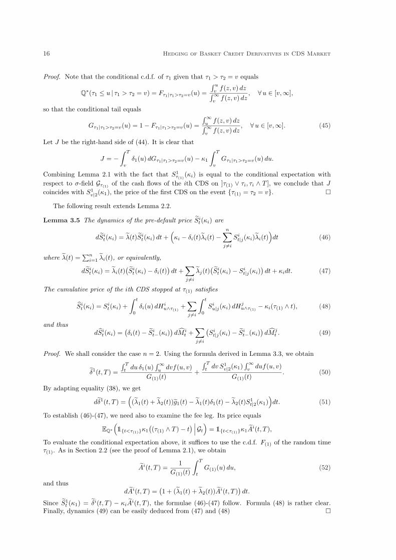
The following result extends Lemma 2.2.

Lemma 3.5 The dynamics of the pre-default price Sit(κi) are

dSit(κi) = λ(t)Si

t(κi) dt +(κi − δi(t)λi(t)−

n∑

j 6=i

Sit|j(κi)λi(t)

)dt (46)

where λ(t) =∑n

i=1 λi(t), or equivalently,

dSit(κi) = λi(t)

(Si

t(κi)− δi(t))dt +

∑

j 6=i

λj(t)(Si

t(κi)− Sit|j(κi)

)dt + κidt. (47)

The cumulative price of the ith CDS stopped at τ(1) satisfies

Sit(κi) = Si

t(κi) +∫ t

0

δi(u) dHiu∧τ(1)

+∑

j 6=i

∫ t

0

Siu|j(κi) dHj

u∧τ(1)− κi(τ(1) ∧ t), (48)

and thusdSi

t(κi) =(δi(t)− Si

t−(κi))dM i

t +∑

j 6=i

(Si

t|j(κi)− Sit−(κi)

)dM j

t . (49)

Proof. We shall consider the case n = 2. Using the formula derived in Lemma 3.3, we obtain

δ1(t, T ) =

∫ T

tdu δ1(u)

∫∞u

dvf(u, v)G(1)(t)

+

∫ T

tdv S1

v|2(κ1)∫∞

vduf(u, v)

G(1)(t). (50)

By adapting equality (38), we get

dδ1(t, T ) =((λ1(t) + λ2(t))g1(t)− λ1(t)δ1(t)− λ2(t)S1

t|2(κ1))dt. (51)

To establish (46)-(47), we need also to examine the fee leg. Its price equals

EQ∗(1t<τ(1)κ1

((τ(1) ∧ T )− t

) ∣∣∣Gt

)= 1t<τ(1)κ1A

i(t, T ),

To evaluate the conditional expectation above, it suffices to use the c.d.f. F(1) of the random timeτ(1). As in Section 2.2 (see the proof of Lemma 2.1), we obtain

Ai(t, T ) =1

G(1)(t)

∫ T

t

G(1)(u) du, (52)

and thusdAi(t, T ) =

(1 + (λ1(t) + λ2(t))Ai(t, T )

)dt.

Since S1t (κ1) = δi(t, T ) − κiA

i(t, T ), the formulae (46)-(47) follow. Formula (48) is rather clear.Finally, dynamics (49) can be easily deduced from (47) and (48) ¤


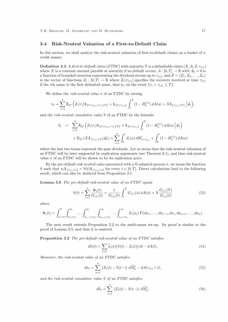
3.4 Risk-Neutral Valuation of a First-to-Default Claim

In this section, we shall analyze the risk-neutral valuation of first-to-default claims on a basket of ncredit names.

Definition 3.2 A first-to-default claim (FTDC) with maturity T is a defaultable claim (X, A, Z, τ(1))where X is a constant amount payable at maturity if no default occurs, A : [0, T ] → R with A0 = 0 isa function of bounded variation representing the dividend stream up to τ(1), and Z = (Z1, Z2, . . . , Zn)is the vector of functions Zi : [0, T ] → R where Zi(τ(1)) specifies the recovery received at time τ(1)

if the ith name is the first defaulted name, that is, on the event τi = τ(1) ≤ T.

We define the risk-neutral value π of an FTDC by setting

πt =n∑

i=1

EQ∗(Zi(τi)1t<τ(1)=τi≤T + 1t<τ(1)

∫ T

t

(1−H(1)u ) dA(u) + X1τ(1)>T

∣∣∣Gt

),

and the risk-neutral cumulative value π of an FTDC by the formula

πt =n∑

i=1

EQ∗(Zi(τi)1t<τ(1)=τi≤T + 1t<τ(1)

∫ T

t

(1−H(1)u ) dA(u)

∣∣∣Gt

)

+ EQ∗(X1τ(1)>T|Gt) +n∑

i=1

∫ t

0

Zi(u) dHiu∧τ(1)

+∫ t

0

(1−H(1)u ) dA(u)

where the last two terms represent the past dividends. Let us stress that the risk-neutral valuation ofan FTDC will be later supported by replication arguments (see Theorem 3.1), and thus risk-neutralvalue π of an FTDC will be shown to be its replication price.

By the pre-default risk-neutral value associated with a G-adapted process π, we mean the functionπ such that πt1τ(1)>t = π(t)1τ(1)>t for every t ∈ [0, T ]. Direct calculations lead to the followingresult, which can also be deduced from Proposition 3.1.

Lemma 3.6 The pre-default risk-neutral value of an FTDC equals

π(t) =n∑

i=1

Ψi(t)G(1)(t)

+1

G(1)(t)

∫ T

t

G(1)(u) dA(u) + XG(1)(T )G(1)(t)

(53)

where

Ψi(t) =∫ T

ui=t

∫ ∞

u1=ui

. . .

∫ ∞

ui−1=ui

∫ ∞

ui+1=ui

. . .

∫ ∞

un=ui

Zi(ui)F (du1, . . . , dui−1, dui, dui+1, . . . , dun).

The next result extends Proposition 2.2 to the multi-name set-up. Its proof is similar to theproof of Lemma 3.5, and thus it is omitted.

Proposition 3.2 The pre-default risk-neutral value of an FTDC satisfies

dπ(t) =∑

i=1

λi(t)(π(t)− Zi(t)

)dt− dA(t). (54)

Moreover, the risk-neutral value of an FTDC satisfies

dπt =n∑

i=1

(Zi(t)− π(t−)) dM iu − dA(τ(1) ∧ t), (55)

and the risk-neutral cumulative value π of an FTDC satisfies

dπt =n∑

i=1

(Zi(t)− π(t−)) dM iu. (56)


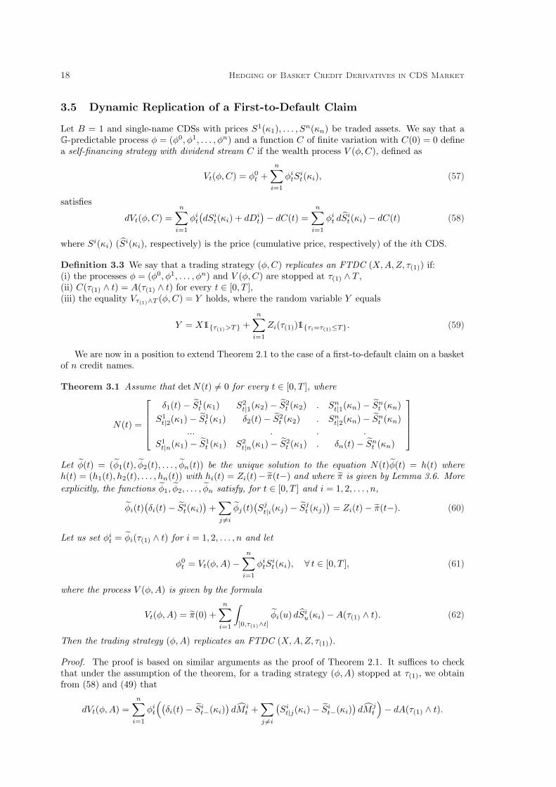
3.5 Dynamic Replication of a First-to-Default Claim

Let B = 1 and single-name CDSs with prices S1(κ1), . . . , Sn(κn) be traded assets. We say that aG-predictable process φ = (φ0, φ1, . . . , φn) and a function C of finite variation with C(0) = 0 definea self-financing strategy with dividend stream C if the wealth process V (φ,C), defined as

Vt(φ,C) = φ0t +

n∑

i=1

φitS

it(κi), (57)

satisfies

dVt(φ,C) =n∑

i=1

φit

(dSi

t(κi) + dDit

)− dC(t) =n∑

i=1

φit dSi

t(κi)− dC(t) (58)

where Si(κi) (Si(κi), respectively) is the price (cumulative price, respectively) of the ith CDS.

Definition 3.3 We say that a trading strategy (φ, C) replicates an FTDC (X,A, Z, τ(1)) if:(i) the processes φ = (φ0, φ1, . . . , φn) and V (φ,C) are stopped at τ(1) ∧ T ,(ii) C(τ(1) ∧ t) = A(τ(1) ∧ t) for every t ∈ [0, T ],(iii) the equality Vτ(1)∧T (φ, C) = Y holds, where the random variable Y equals

Y = X1τ(1)>T +n∑

i=1

Zi(τ(1))1τi=τ(1)≤T. (59)

We are now in a position to extend Theorem 2.1 to the case of a first-to-default claim on a basketof n credit names.

Theorem 3.1 Assume that detN(t) 6= 0 for every t ∈ [0, T ], where

N(t) =

δ1(t)− S1t (κ1) S2

t|1(κ2)− S2t (κ2) . Sn

t|1(κn)− Snt (κn)

S1t|2(κ1)− S1

t (κ1) δ2(t)− S2t (κ2) . Sn

t|2(κn)− Snt (κn)

... . . .

S1t|n(κ1)− S1

t (κ1) S2t|n(κ1)− S2

t (κ1) . δn(t)− Snt (κn)

Let φ(t) = (φ1(t), φ2(t), . . . , φn(t)) be the unique solution to the equation N(t)φ(t) = h(t) whereh(t) = (h1(t), h2(t), . . . , hn(t)) with hi(t) = Zi(t)− π(t−) and where π is given by Lemma 3.6. Moreexplicitly, the functions φ1, φ2, . . . , φn satisfy, for t ∈ [0, T ] and i = 1, 2, . . . , n,

φi(t)(δi(t)− Si

t(κi))

+∑

j 6=i

φj(t)(Sj

t|i(κj)− Sjt (κj)

)= Zi(t)− π(t−). (60)

Let us set φit = φi(τ(1) ∧ t) for i = 1, 2, . . . , n and let

φ0t = Vt(φ,A)−

n∑

i=1

φitS

it(κi), ∀ t ∈ [0, T ], (61)

where the process V (φ,A) is given by the formula

Vt(φ,A) = π(0) +n∑

i=1

∫

]0,τ(1)∧t]

φi(u) dSiu(κi)−A(τ(1) ∧ t). (62)

Then the trading strategy (φ,A) replicates an FTDC (X, A, Z, τ(1)).

Proof. The proof is based on similar arguments as the proof of Theorem 2.1. It suffices to checkthat under the assumption of the theorem, for a trading strategy (φ,A) stopped at τ(1), we obtainfrom (58) and (49) that

dVt(φ,A) =n∑

i=1

φit

((δi(t)− Si

t−(κi))dM i

t +∑

j 6=i

(Si

t|j(κi)− Sit−(κi)

)dM j

t

)− dA(τ(1) ∧ t).


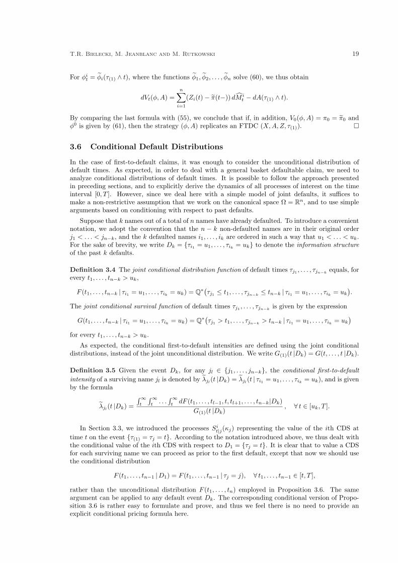
For φit = φi(τ(1) ∧ t), where the functions φ1, φ2, . . . , φn solve (60), we thus obtain

dVt(φ,A) =n∑

i=1

(Zi(t)− π(t−)) dM it − dA(τ(1) ∧ t).

By comparing the last formula with (55), we conclude that if, in addition, V0(φ, A) = π0 = π0 andφ0 is given by (61), then the strategy (φ, A) replicates an FTDC (X, A, Z, τ(1)). ¤

3.6 Conditional Default Distributions

In the case of first-to-default claims, it was enough to consider the unconditional distribution ofdefault times. As expected, in order to deal with a general basket defaultable claim, we need toanalyze conditional distributions of default times. It is possible to follow the approach presentedin preceding sections, and to explicitly derive the dynamics of all processes of interest on the timeinterval [0, T ]. However, since we deal here with a simple model of joint defaults, it suffices tomake a non-restrictive assumption that we work on the canonical space Ω = Rn, and to use simplearguments based on conditioning with respect to past defaults.

Suppose that k names out of a total of n names have already defaulted. To introduce a convenientnotation, we adopt the convention that the n − k non-defaulted names are in their original orderj1 < . . . < jn−k, and the k defaulted names i1, . . . , ik are ordered in such a way that u1 < . . . < uk.For the sake of brevity, we write Dk = τi1 = u1, . . . , τik

= uk to denote the information structureof the past k defaults.

Definition 3.4 The joint conditional distribution function of default times τj1 , . . . , τjn−kequals, for

every t1, . . . , tn−k > uk,

F (t1, . . . , tn−k | τi1 = u1, . . . , τik= uk) = Q∗

(τj1 ≤ t1, . . . , τjn−k

≤ tn−k | τi1 = u1, . . . , τik= uk

).

The joint conditional survival function of default times τj1 , . . . , τjn−kis given by the expression

G(t1, . . . , tn−k | τi1 = u1, . . . , τik= uk) = Q∗

(τj1 > t1, . . . , τjn−k

> tn−k | τi1 = u1, . . . , τik= uk

)

for every t1, . . . , tn−k > uk.

As expected, the conditional first-to-default intensities are defined using the joint conditionaldistributions, instead of the joint unconditional distribution. We write G(1)(t |Dk) = G(t, . . . , t |Dk).

Definition 3.5 Given the event Dk, for any jl ∈ j1, . . . , jn−k, the conditional first-to-defaultintensity of a surviving name jl is denoted by λjl

(t |Dk) = λjl(t | τi1 = u1, . . . , τik

= uk), and is givenby the formula

λjl(t |Dk) =

∫∞t

∫∞t

. . .∫∞

tdF (t1, . . . , tl−1, t, tl+1, . . . , tn−k|Dk)

G(1)(t |Dk), ∀ t ∈ [uk, T ].

In Section 3.3, we introduced the processes Sit|j(κj) representing the value of the ith CDS at

time t on the event τ(1) = τj = t. According to the notation introduced above, we thus dealt withthe conditional value of the ith CDS with respect to D1 = τj = t. It is clear that to value a CDSfor each surviving name we can proceed as prior to the first default, except that now we should usethe conditional distribution

F (t1, . . . , tn−1 |D1) = F (t1, . . . , tn−1 | τj = j), ∀ t1, . . . , tn−1 ∈ [t, T ],

rather than the unconditional distribution F (t1, . . . , tn) employed in Proposition 3.6. The sameargument can be applied to any default event Dk. The corresponding conditional version of Propo-sition 3.6 is rather easy to formulate and prove, and thus we feel there is no need to provide anexplicit conditional pricing formula here.


The conditional first-to-default intensities introduced in Definition 3.5 will allow us to constructthe conditional first-to-default martingales in a similar way as we defined the first-to-default mar-tingales M i associated with the first-to-default intensities λi. However, since any name can defaultat any time, we need to introduce an entire family of conditional martingales, whose compensatorsare based on intensities conditioned on the information structure of past defaults.

Definition 3.6 Given the default event Dk = τi1 = u1, . . . , τik= uk, for each surviving name

jl ∈ j1, . . . , jn−k, we define the basic conditional first-to-default martingale M jl

t|Dkby setting

M jl

t|Dk= Hjl

t∧τ(k+1)−

∫ t

uk

1u<τ(k+1)λjl(u |Dk) du, ∀ t ∈ [uk, T ]. (63)

The process M jl

t|Dk, t ∈ [uk, T ], is a martingale under the conditioned probability measure Q∗|Dk,

that is, the probability measure Q∗ conditioned on the event Dk, and with respect to the filtrationgenerated by default processes of the surviving names, that is, the filtration GDk

t := Hj1t ∨ . . .∨Hjn−k

t

for t ∈ [uk, T ].

Since we condition on the event Dk, we have τ(k+1) = τj1 ∧ τj2 ∧ . . .∧ τjn−k, so that τ(k+1) is the

first default for all surviving names. Formula (63) is thus a rather straightforward generalization offormula (33). In particular, for k = 0 we obtain M i

t|D0= M i

t , t ∈ [0, T ], for any i = 1, 2, . . . , n. The

martingale property of the process M jl

t|Dk, stated in Definition 3.6, follows from Proposition 3.3 (it

can also be seen as a conditional version of Corollary 3.1).

We are in the position to state the conditional version of the first-to-default martingale repre-sentation theorem of Section 3.2. Formally, this result is nothing else than a restatement of themartingale representation formula of Proposition 3.1 in terms of conditional first-to-default intensi-ties and conditional first-to-default martingales.

Let us fix an event Dk write GDk = Hj1 ∨ . . . ∨Hjn−k .

Proposition 3.3 Let Y be a random variable given by the formula

Y =n−k∑

l=1

Zjl|Dk(τjl

)1τjl≤T, τjl

=τ(k+1) + X1τ(k+1)>T (64)

for some functions Zjl|Dk: [uk, T ] → R, l = 1, 2, . . . , n−k, and some constant X (possibly dependent

on Dk). Let us defineMt|Dk

= EQ∗|Dk(Y | GDk

t ), ∀ t ∈ [uk, T ]. (65)

Then Mt|Dk, t ∈ [uk, T ], is a GDk -martingale with respect to the conditioned probability measure

Q∗|Dk and it admits the following representation, for t ∈ [uk, T ],

Mt|Dk= M0|Dk

+n−k∑

l=1

∫

]uk,t]

hjl(u|Dk) dM jl

u|Dk

where the processes hjlare given by

hjl(t |Dk) = Zjl|Dk

(t)− Mt−|Dk, ∀ t ∈ [uk, T ].

Proof. The proof relies on a direct extension of arguments used in the proof of Proposition 3.1 tothe context of conditional default distributions. Therefore, it is left to the reader. ¤

3.7 Recursive Valuation of a Basket Claim

We are ready extend the results developed in the context of first-to-default claims to value and hedgegeneral basket claims. A generic basket claim is any contingent claim that pays a specified amounton each default from a basket of n credit names and a constant amount at maturity T if no defaultshave occurred prior to or at T .


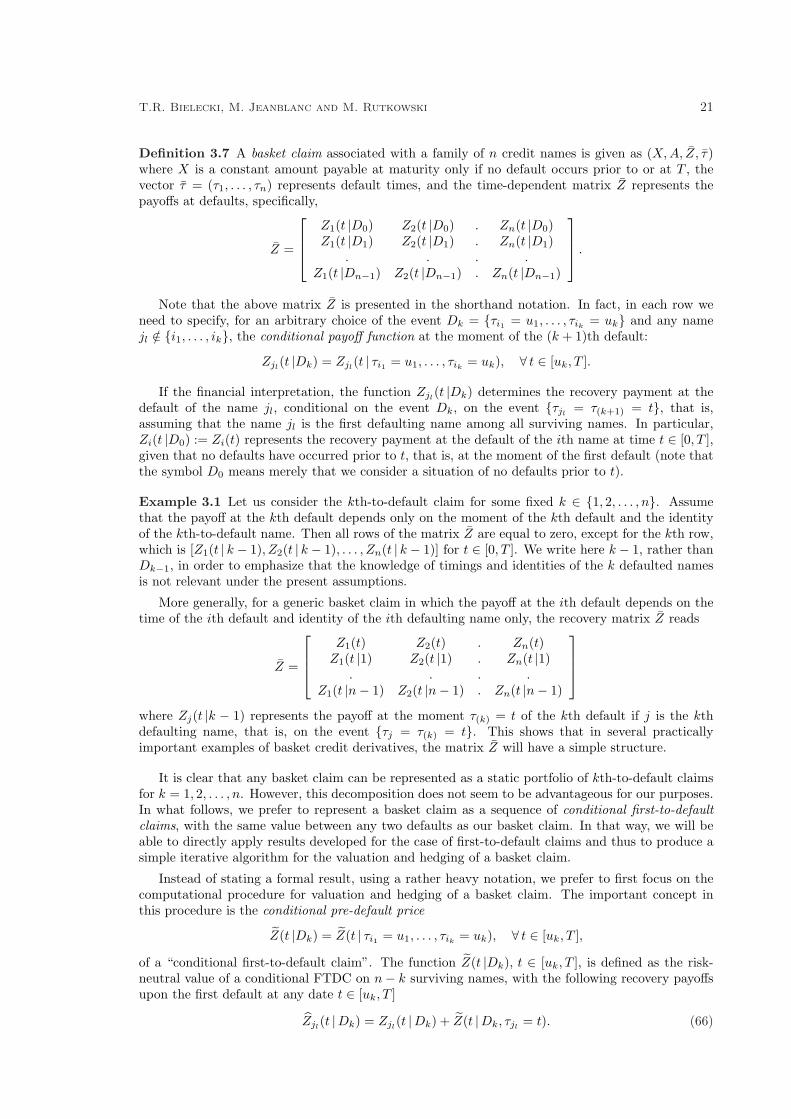
Definition 3.7 A basket claim associated with a family of n credit names is given as (X, A, Z, τ)where X is a constant amount payable at maturity only if no default occurs prior to or at T , thevector τ = (τ1, . . . , τn) represents default times, and the time-dependent matrix Z represents thepayoffs at defaults, specifically,

Z =

Z1(t |D0) Z2(t |D0) . Zn(t |D0)Z1(t |D1) Z2(t |D1) . Zn(t |D1)

. . . .Z1(t |Dn−1) Z2(t |Dn−1) . Zn(t |Dn−1)

.

Note that the above matrix Z is presented in the shorthand notation. In fact, in each row weneed to specify, for an arbitrary choice of the event Dk = τi1 = u1, . . . , τik

= uk and any namejl /∈ i1, . . . , ik, the conditional payoff function at the moment of the (k + 1)th default:

Zjl(t |Dk) = Zjl

(t | τi1 = u1, . . . , τik= uk), ∀ t ∈ [uk, T ].

If the financial interpretation, the function Zjl(t |Dk) determines the recovery payment at the

default of the name jl, conditional on the event Dk, on the event τjl= τ(k+1) = t, that is,

assuming that the name jl is the first defaulting name among all surviving names. In particular,Zi(t |D0) := Zi(t) represents the recovery payment at the default of the ith name at time t ∈ [0, T ],given that no defaults have occurred prior to t, that is, at the moment of the first default (note thatthe symbol D0 means merely that we consider a situation of no defaults prior to t).

Example 3.1 Let us consider the kth-to-default claim for some fixed k ∈ 1, 2, . . . , n. Assumethat the payoff at the kth default depends only on the moment of the kth default and the identityof the kth-to-default name. Then all rows of the matrix Z are equal to zero, except for the kth row,which is [Z1(t | k − 1), Z2(t | k − 1), . . . , Zn(t | k − 1)] for t ∈ [0, T ]. We write here k − 1, rather thanDk−1, in order to emphasize that the knowledge of timings and identities of the k defaulted namesis not relevant under the present assumptions.

More generally, for a generic basket claim in which the payoff at the ith default depends on thetime of the ith default and identity of the ith defaulting name only, the recovery matrix Z reads

Z =

Z1(t) Z2(t) . Zn(t)Z1(t |1) Z2(t |1) . Zn(t |1)

. . . .Z1(t |n− 1) Z2(t |n− 1) . Zn(t |n− 1)

where Zj(t |k − 1) represents the payoff at the moment τ(k) = t of the kth default if j is the kthdefaulting name, that is, on the event τj = τ(k) = t. This shows that in several practicallyimportant examples of basket credit derivatives, the matrix Z will have a simple structure.

It is clear that any basket claim can be represented as a static portfolio of kth-to-default claimsfor k = 1, 2, . . . , n. However, this decomposition does not seem to be advantageous for our purposes.In what follows, we prefer to represent a basket claim as a sequence of conditional first-to-defaultclaims, with the same value between any two defaults as our basket claim. In that way, we will beable to directly apply results developed for the case of first-to-default claims and thus to produce asimple iterative algorithm for the valuation and hedging of a basket claim.

Instead of stating a formal result, using a rather heavy notation, we prefer to first focus on thecomputational procedure for valuation and hedging of a basket claim. The important concept inthis procedure is the conditional pre-default price

Z(t |Dk) = Z(t | τi1 = u1, . . . , τik= uk), ∀ t ∈ [uk, T ],

of a “conditional first-to-default claim”. The function Z(t |Dk), t ∈ [uk, T ], is defined as the risk-neutral value of a conditional FTDC on n− k surviving names, with the following recovery payoffsupon the first default at any date t ∈ [uk, T ]

Zjl(t |Dk) = Zjl

(t |Dk) + Z(t |Dk, τjl= t). (66)


Assume for the moment that for any name jm /∈ i1, . . . , ik, jl the conditional recovery payoffZjm

(t | τi1 = u1, . . . , τik= uk, τjl

= uk+1) upon the first default after date uk+1 is known. Then wecan compute the function

Z(t | τi1 = u1, . . . , τik= uk, τjl

= uk+1), ∀ t ∈ [uk+1, T ],

as in Lemma 3.6, but using conditional default distribution. The assumption that the conditionalpayoffs are known is in fact not restrictive, since the functions appearing in right-hand side of (66)are known from the previous step in the following recursive pricing algorithm.

• First step. We first derive the value of a basket claim assuming that all but one defaults havealready occurred. Let Dn−1 = τi1 = u1, . . . , τin−1 = un−1. For any t ∈ [un−1, T ], we dealwith the payoffs

Zj1(t |Dn−1) = Zj1(t |Dn−1) = Zj1(t | τi1 = u1, . . . , τin−1 = un−1),

for j1 /∈ i1, . . . , in−1 where the recovery payment function Zj1(t |Dn−1), t ∈ [un−1, T ], isgiven by the specification of the basket claim. Hence we can evaluate the pre-default valueZ(t |Dn−1) at any time t ∈ [un−1, T ], as a value of a conditional first-to-default claim with thesaid payoff, using the conditional distribution under Q∗|Dn−1 of the random time τj1 = τin onthe interval [un−1, T ].

• Second step. In this step, we assume that all but two names have already defaulted. LetDn−2 = τi1 = u1, . . . , τin−2 = un−2. For each surviving name j1, j2 /∈ i1, . . . , in−2, thepayoff Zjl

(t |Dn−2), t ∈ [un−2, T ], of a basket claim at the moment of the next default for-mally comprises the recovery payoff from the defaulted name jl which is Zjl

(t |Dn−2) andthe pre-default value Z(t |Dn−2, τjl

= t), t ∈ [un−2, T ], which was computed in the first step.Therefore, we have

Zjl(t |Dn−2) = Zjl

(t |Dn−2) + Z(t |Dn−2, τjl= t), ∀ t ∈ [un−2, T ].

To find the value of a basket claim between the (n − 2)th and (n − 1)th default, it sufficesto compute the pre-default value of the conditional FTDC associated with the two survivingnames, j1, j2 /∈ i1, . . . , in−2. Since the conditional payoffs Zj1(t |Dn−2) and Zj2(t |Dn−2) areknown, we may compute the expectation under the conditional probability measure Q∗|Dn−2

in order to find the pre-default value of this conditional FTDC for any t ∈ [un−2, T ].

• General induction step. We now assume that exactly k default have occurred, that is, weassume that the event Dk = τi1 = u1, . . . , τik

= uk is given. From the preceding step, weknow the function Z(t |Dk+1) where Dk = τi1 = u1, . . . , τik

= uk, τjl= uk+1. In order to

compute Z(t |Dk), we set

Zjl(t |Dk) = Zjl

(t |Dk) + Z(t |Dk, τjl= t), ∀ t ∈ [uk, T ], (67)

for any j1, . . . , jn−k /∈ i1, . . . , ik, and we compute Z(t |Dk), t ∈ [uk, T ], as the risk-neutralvalue under Q∗|Dk at time of the conditional FTDC with the payoffs given by (67).

We are in the position state the valuation result for a basket claim, which can be formally provedusing the reasoning presented above.

Proposition 3.4 The risk-neutral value at time t ∈ [0, T ] of a basket claim (X, A, Z, τ) equals

πt =n−1∑

k=0

Z(t |Dk)1[τ(k)∧T,τ(k+1)∧T [(t), ∀ t ∈ [0, T ],

where Dk = Dk(ω) = τi1(ω) = u1, . . . , τik(ω) = uk for k = 1, 2, . . . , n, and D0 means that no

defaults have yet occurred.


3.8 Recursive Replication of a Basket Claim

From the discussion of the preceding section, it is clear that a basket claim can be convenientlyinterpreted as a specific sequence of conditional first-to-default claims. Hence it is easy to guess thatthe replication of a basket claim should refer to hedging of the underlying sequence of conditionalfirst-to-default claims. In the next result, we denote τ(0) = 0.

Theorem 3.2 For any k = 0, 1, . . . , n, the replicating strategy φ for a basket claim (X, A, Z, τ)on the time interval [τk ∧ T, τk+1 ∧ T ] coincides with the replicating strategy for the conditionalFTDC with payoffs Z(t |Dk) given by (67). The replicating strategy φ = (φ0, φj1, . . . , φjn−k , A),corresponding to the units of savings account and units of CDS on each surviving name at time t,has the wealth process

Vt(φ,A) = φ0t +

n−i∑

l=1

φjlt Sjl

t (κjl)

where processes φjl , l = 1, 2, . . . , n− k can be computed by the conditional version of Theorem 3.1.

Proof. We know that the basket claim can be decomposed into a series of conditional first-to-default claims. So, at any given moment of time t ∈ [0, T ], assuming that k defaults have alreadyoccurred, our basket claim is equivalent to the conditional FTDC with payoffs Z(t |Dk) and thepre-default value Z(t |Dk). This conditional FTDC is alive up to the next default τ(k+1) or maturityT , whichever comes first. Hence it is clear that the replicating strategy of a basket claim over therandom interval [τk ∧ T, τk+1 ∧ T ] need to coincide with the replicating strategy for this conditionalfirst-to-default claim, and thus it can be found along the same lines as in Theorem 3.1, using theconditional distribution under Q∗|Dk of defaults for surviving names. ¤

4 Applications to Copula-Based Credit Risk Models

In this section, we will apply our previous results to some specific models, in which some commoncopulas are used to model dependence between default times (see, for instance, Cherubini et al. [7],Embrechts et al. [8], Frey et al. [9], Laurent and Gregory [12], Li [13] or McNeil et al. [14]). It isfair to admit that copula-based credit risk models are not fully suitable for a dynamical approachto credit risk, since the future behavior of credit spreads can be predicted with certainty, up tothe observations of default times. Hence they are unsuitable for hedging of option-like contracts oncredit spreads. On the other hand, however, these models are of a common use in practical valuationcredit derivatives and thus we decided to present them here. Of course, our results are more general,so that they can be applied to an arbitrary joint distribution of default times (i.e., not necessarilygiven by some copula function). Also, in the follow-up work [2] we extend the results of this workto a fully dynamical set-up.

For simplicity of exposition and in order to get more explicit formulae, we only consider thebivariate situation and we make the following standing assumptions.

Assumptions (B). We assume from now on that:(i) we are given an FTDC (X,A, Z, τ(1)) where Z = (Z1, Z2) for some constants Z1, Z2 and X,(ii) the default times τ1 and τ2 have exponential marginal distributions with parameters λ1 and λ2,(ii) the recovery δi of the ith CDS is constant and κi = λiδi for i = 1, 2 (see Example 2.1).

Before proceeding to computations, let us note that∫ T

u=t

∫ ∞

v=u

G(du, dv) = −∫ T

t

G(du, u)

and thus, assuming that the pair (τ1, τ2) has the joint probability density function f(u, v),∫ T

t

du

∫ ∞

u

dvf(u, v) = −∫ T

t

∂1G(u, u) du


and

dv

∫ b

a

f(u, v) du = G(a, dv)−G(b, dv) = dv(∂2G(b, v)− ∂2G(a, v)

)

∫ T

v

du

∫ ∞

u

dzf(z, v) = −∫ T

v

∂2G(u, v) du.

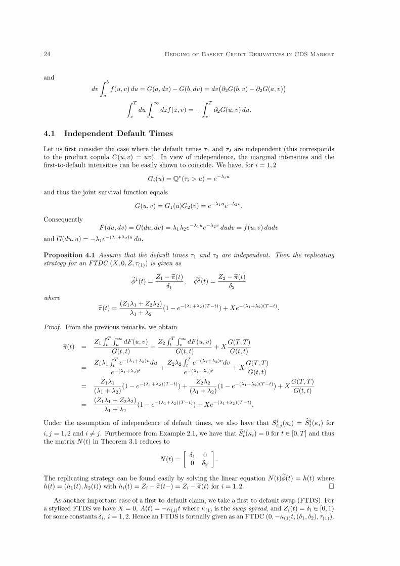
4.1 Independent Default Times

Let us first consider the case where the default times τ1 and τ2 are independent (this correspondsto the product copula C(u, v) = uv). In view of independence, the marginal intensities and thefirst-to-default intensities can be easily shown to coincide. We have, for i = 1, 2

Gi(u) = Q∗(τi > u) = e−λiu

and thus the joint survival function equals

G(u, v) = G1(u)G2(v) = e−λ1ue−λ2v.

ConsequentlyF (du, dv) = G(du, dv) = λ1λ2e

−λ1ue−λ2v dudv = f(u, v) dudv

and G(du, u) = −λ1e−(λ1+λ2)u du.

Proposition 4.1 Assume that the default times τ1 and τ2 are independent. Then the replicatingstrategy for an FTDC (X, 0, Z, τ(1)) is given as

φ1(t) =Z1 − π(t)

δ1, φ2(t) =

Z2 − π(t)δ2

where

π(t) =(Z1λ1 + Z2λ2)

λ1 + λ2(1− e−(λ1+λ2)(T−t)) + Xe−(λ1+λ2)(T−t).

Proof. From the previous remarks, we obtain

π(t) =Z1

∫ T

t

∫∞u

dF (u, v)G(t, t)

+Z2

∫ T

t

∫∞v

dF (u, v)G(t, t)

+ XG(T, T )G(t, t)

=Z1λ1

∫ T

te−(λ1+λ2)udu

e−(λ1+λ2)t+

Z2λ2

∫ T

te−(λ1+λ2)vdv

e−(λ1+λ2)t+ X

G(T, T )G(t, t)

=Z1λ1

(λ1 + λ2)(1− e−(λ1+λ2)(T−t)) +

Z2λ2

(λ1 + λ2)(1− e−(λ1+λ2)(T−t)) + X

G(T, T )G(t, t)

=(Z1λ1 + Z2λ2)

λ1 + λ2(1− e−(λ1+λ2)(T−t)) + Xe−(λ1+λ2)(T−t).

Under the assumption of independence of default times, we also have that Sit|j(κi) = Si

t(κi) for

i, j = 1, 2 and i 6= j. Furthermore from Example 2.1, we have that Sit(κi) = 0 for t ∈ [0, T ] and thus

the matrix N(t) in Theorem 3.1 reduces to

N(t) =[

δ1 00 δ2

].

The replicating strategy can be found easily by solving the linear equation N(t)φ(t) = h(t) whereh(t) = (h1(t), h2(t)) with hi(t) = Zi − π(t−) = Zi − π(t) for i = 1, 2. ¤

As another important case of a first-to-default claim, we take a first-to-default swap (FTDS). Fora stylized FTDS we have X = 0, A(t) = −κ(1)t where κ(1) is the swap spread, and Zi(t) = δi ∈ [0, 1)for some constants δi, i = 1, 2. Hence an FTDS is formally given as an FTDC (0,−κ(1)t, (δ1, δ2), τ(1)).


Under the present assumptions, we easily obtain

π0 = π(0) =1− eλT

λ

((λ1δ1 + λ2δ2)− κ(1)

)

where λ = λ1 + λ2. The FTDS market spread is the level of κ(1) that makes the FTDS valueless atinitiation. Hence in this elementary example this spread equals λ1δ1 + λ2δ2. In addition, it can beshown that under the present assumptions we have that π(t) = 0 for every t ∈ [0, T ].

Suppose that we wish to hedge the short position in the FTDS using two CDSs, say CDSi,i = 1, 2, with respective default times τi, protection payments δi and spreads κi = λiδi. Recall thatin the present set-up we have that, for t ∈ [0, T ],

Sit|j(κi) = Si

t(κi) = 0, i, j = 1, 2, i 6= j. (68)

Consequently, we have here that hi(t) = −Zi(t) = −δi for every t ∈ [0, T ]. It then follows fromequation N(t)φ(t) = h(t) that φ1(t) = φ2(t) = 1 for every t ∈ [0, T ] and thus φ0

t = 0 for everyt ∈ [0, T ]. This result is by no means surprising: we hedge a short position in the FTDS byholding a static portfolio of two single-name CDSs since, under the present assumptions, the FTDSis equivalent to such a portfolio of corresponding single name CDSs. Of course, one would not expectthat this feature will still hold in a general case of dependent default times.

The first equality in (68) is due to the standing assumption of independence of default times τ1

and τ2 and thus it will no longer be true for other copulas (see foregoing subsections). The secondequality follows from the postulate that the risk-neutral marginal distributions of default times areexponential. In practice, the risk-neutral marginal distributions of default times will be obtained byfitting the model to market data (i.e., market prices of single name CDSs) and thus typically theywill not be exponential. To conclude, both equalities in (68) are unlikely to hold in any real-lifeimplementation. Hence this example show be seen as the simplest illustration of general results andwe do not pretend that it has any practical merits. Nevertheless, we believe that it might be usefulto give a few more comments on the hedging strategy considered in this example.

Suppose that a dealer sells one FTDS and hedges his short position by holding a portfoliocomposed of one CDS1 contract and one CDS2 contract. Let us consider the event τ(1) = τ1 < T.The cumulative premium the dealer collects on the time interval [0, t], t ≤ τ(1), for selling the FTDSequals (λ1δ1 + λ2δ2)t. The protection coverage that the dealer has to pay at time τ(1) equals δ1 andthe FTDS is terminated at τ1. Now, the cumulative premium the dealer pays on the time interval[0, t], t ≤ τ(1), for holding the portfolio of one CDS1 contract and one CDS2 contract is (λ1δ1+λ2δ2)t.At time τ1, the dealer receives the protection payment of δ1. The CDS1 is terminated at time τ1;the dealer still holds the CDS2 contract, however. Recall, though, that the ex-dividend price (i.e.,the market price) of this contract is zero. Hence the dealer may unwind the contract at time τ(1) atno cost (again, this only holds under the assumption of independence and exponential marginals).Consequently the dealer’s P/L is flat (zero) over the lifetime of the FTDS and the dealer has nopositions in the remaining CDS at the first default time. Though we consider here the simplestset-up, it is plausible that a similar interpretation of a hedging strategy will also apply in a moregeneral framework.

4.2 Archimedean Copulas

We now proceed to the case of exponentially distributed, but dependent, default times. Theirinterdependence will be specified by a choice of some Archimedean copula. Such examples werestudied by Hua [11]; we present and simplify here some of his computations. Recall that a bivariateArchimedean copula is defined as

C(u, v) = ϕ−1(ϕ(u), ϕ(v))

where ϕ is called the generator of a copula.


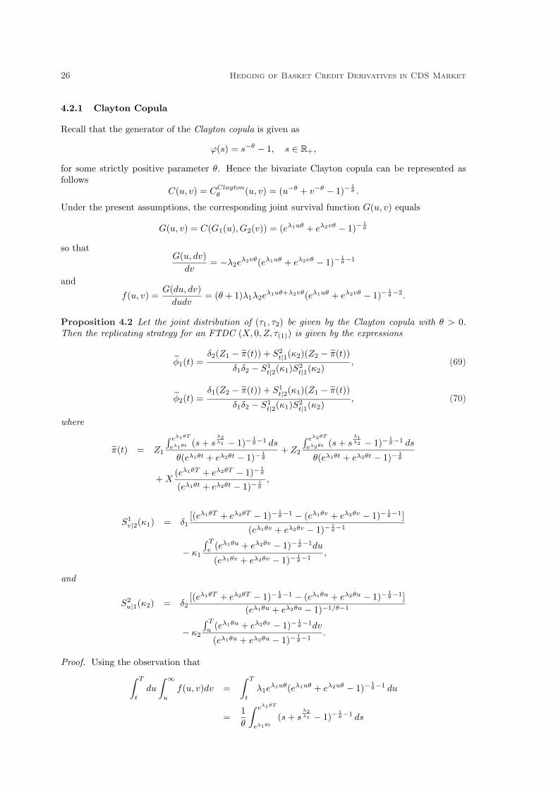
4.2.1 Clayton Copula

Recall that the generator of the Clayton copula is given as

ϕ(s) = s−θ − 1, s ∈ R+,

for some strictly positive parameter θ. Hence the bivariate Clayton copula can be represented asfollows

C(u, v) = CClaytonθ (u, v) = (u−θ + v−θ − 1)−

1θ .

Under the present assumptions, the corresponding joint survival function G(u, v) equals

G(u, v) = C(G1(u), G2(v)) = (eλ1uθ + eλ2vθ − 1)−1θ

so thatG(u, dv)

dv= −λ2e

λ2vθ(eλ1uθ + eλ2vθ − 1)−1θ−1

and

f(u, v) =G(du, dv)

dudv= (θ + 1)λ1λ2e

λ1uθ+λ2vθ(eλ1uθ + eλ2vθ − 1)−1θ−2.

Proposition 4.2 Let the joint distribution of (τ1, τ2) be given by the Clayton copula with θ > 0.Then the replicating strategy for an FTDC (X, 0, Z, τ(1)) is given by the expressions

φ1(t) =δ2(Z1 − π(t)) + S2

t|1(κ2)(Z2 − π(t))

δ1δ2 − S1t|2(κ1)S2

t|1(κ2), (69)

φ2(t) =δ1(Z2 − π(t)) + S1

t|2(κ1)(Z1 − π(t))

δ1δ2 − S1t|2(κ1)S2

t|1(κ2), (70)

where

π(t) = Z1

∫ eλ1θT

eλ1θt (s + sλ2λ1 − 1)−

1θ−1 ds

θ(eλ1θt + eλ2θt − 1)−1θ

+ Z2

∫ eλ2θT

eλ2θt (s + sλ1λ2 − 1)−

1θ−1 ds


+ X(eλ1θT + eλ2θT − 1)−

1θ

(eλ1θt + eλ2θt − 1)−1θ

,

S1v|2(κ1) = δ1

[(eλ1θT + eλ2θT − 1)−1θ−1 − (eλ1θv + eλ2θv − 1)−

1θ−1]

(eλ1θv + eλ2θv − 1)−1θ−1

− κ1

∫ T

v(eλ1θu + eλ2θv − 1)−

1θ−1du

(eλ1θv + eλ2θv − 1)−1θ−1

,

and

S2u|1(κ2) = δ2

[(eλ1θT + eλ2θT − 1)−1θ−1 − (eλ1θu + eλ2θu − 1)−

1θ−1]

(eλ1θu + eλ2θu − 1)−1/θ−1

− κ2

∫ T

u(eλ1θu + eλ2θv − 1)−

1θ−1dv

(eλ1θu + eλ2θu − 1)−1θ−1

.

Proof. Using the observation that∫ T

t

du

∫ ∞

u

f(u, v)dv =∫ T

t

λ1eλ1uθ(eλ1uθ + eλ2uθ − 1)−

1θ−1 du

=1θ

∫ eλ1θT

eλ1θt

(s + sλ2λ1 − 1)−

1θ−1 ds


and thus by symmetry∫ T

t

dv

∫ ∞

v

f(u, v)du =1θ

∫ eλ2θT

eλ2θt

(s + sλ1λ2 − 1)−

1θ−1 ds.

We thus obtain

π(t) =Z1

∫ T

t

∫∞u

dG(u, v)G(t, t)

+Z2

∫ T

t

∫∞v

dG(u, v)G(t, t)

+ XG(T, T )G(t, t)

= Z1

∫ eλ1θT

eλ1θt (s + sλ2λ1 − 1)−

1θ−1 ds


+ Z2

∫ eλ2θT

eλ2θt (s + sλ1λ2 − 1)−

1θ−1 ds


+ X(eλ1θT + eλ2θT − 1)−

1θ

(eλ1θt + eλ2θt − 1)−1θ

.

We are in a position to determine the replicating strategy. Under the standing assumption thatκi = λiδi for i = 1, 2 we still have that Si

t(κi) = 0 for i = 1, 2 and for t ∈ [0, T ]. Hence the matrixN(t) reduces to

N(t) =

[δ1 −S2

t|1(κ2)−S1

t|2(κ1) δ2

]

where

S1v|2(κ1) = δ1

∫ T

vf(u, v) du∫∞

vf(u, v) du

− κ1

∫ T

v

∫∞u

f(z, v) dzdu∫∞v

f(u, v) du

= δ1G(T, dv)−G(v, dv)

G(v, dv)+ κ1

∫ T

tG(u, dv)

G(v, dv)

= δ1[(eλ1θT + eλ2θT − 1)−

1θ−1 − (eλ1θv + eλ2θv − 1)−

1θ−1]

(eλ1θv + eλ2θv − 1)−1θ−1

− κ1

∫ T

v(eλ1θu + eλ2θv − 1)−

1θ−1 du

(eλ1θv + eλ2θv − 1)−1θ−1

.

The expression for S2u|1(κ2) can be found by analogous computations. By solving the equation

N(t)φ(t) = h(t), we obtain the desired expressions (69)-(70). ¤

Similar computations can be done for the valuation and hedging of a first-to-default swap.

4.2.2 Gumbel Copula

As another of an Archimedean copula, we consider the Gumbel copula with the generator

ϕ(s) = (− ln s)θ, s ∈ R+,

for some θ ≥ 1. The bivariate Gumbel copula can thus be written as

C(u, v) = CGumbelθ (u, v) = e−[(− ln u)θ+(− ln v)θ]

1θ .

Under our standing assumptions, the corresponding joint survival function G(u, v) equals

G(u, v) = C(G1(u), G2(v)) = e−(λθ1uθ+λθ

2vθ)1θ .

ConsequentlydG(u, v)

dv= −G(u, v)λθ

2vθ−1(λθ

1uθ + λθ

2vθ)

1θ−1

anddG(u, v)

dudv= G(u, v)(λ1λ2)θ(uv)θ−1(λθ

1uθ + λθ

2vθ)

1θ−2

((λθ

1uθ + λθ

2vθ)

1θ + θ − 1

).


Proposition 4.3 Let the joint distribution of (τ1, τ2) be given by the Gumbel copula with θ ≥ 1.Then the replicating strategy for an FTDC (X, 0, Z, τ(1)) is given by (69)-(70) with

π(t) = (Z1λθ1 + Z2λ

θ2)λ

−θ(e−λt − e−λT ) + Xe−λ(T−t),

S1v|2(κ1) = δ1

e−(λθ1T θ+λθ

2vθ)1θ (λθ

1Tθ + λθ

2vθ)

1θ−1 − e−λvλ1−θv1−θ

e−λvλ1−θv1−θ

− κ1

∫ T

ve−(λθ

1T θ+λθ2vθ)

1θ (λθ

1uθ + λθ

2vθ)

1θ−1 du

e−λvλ1−θv1−θ,

S2u|1(κ2) = δ2

e−(λθ1uθ+λθ

2T θ)1θ (λθ

1uθ + λθ

2Tθ)

1θ−1 − e−λvλ1−θu1−θ

e−λvλ1−θu1−θ

− κ2

∫ T

ue−(λθ

1uθ+λθ2T θ)

1θ (λθ

1uθ + λθ

2vθ)

1θ−1 dv

e−λvλ1−θu1−θ.

Proof. We have∫ T

t

∫ ∞

u

dG(u, v) =∫ T

t

λθ1(λ

θ1 + λθ

2)1θ−1e−(λθ

1+λθ2)

1θ u du

= (−λθ1λ−θe−λu)|u=T

u=t = λθ1λ−θ(e−λt − e−λT )

where λ = (λθ1 + λθ

2)1θ . Similarly

∫ T

t

∫ ∞

v

dG(u, v) = λθ2λ−θ(e−λt − e−λT ).

Furthermore G(T, T ) = e−λT and G(t, t) = e−λt. Hence

π(t) = Z1

∫ T

t

∫∞u

dG(u, v)G(t, t)

+ Z2

∫ T

t

∫∞v

dG(u, v)G(t, t)

+ XG(T, T )G(t, t)

= Z1λθ1λ−θ(e−λt − e−λT ) + Z2λ

θ2λ−θ(e−λt − e−λT ) + Xe−λ(T−t)

= (Z1λθ1 + δ2Z

θ2 )λ−θ(e−λt − e−λT ) + Xe−λ(T−t).

In order to find the replicating strategy, we proceed as in the proof of Proposition 4.2. Under thepresent assumptions, we have

S1v|2(κ1) = δ1

∫ T

vf(u, v)du∫∞

vf(u, v)du

− κ1

∫ T

v

∫∞u

f(z, v)dzdu∫∞v

f(u, v)du

= δ1e−(λθ

1T θ+λθ2vθ)

1θ (λθ

1Tθ + λθ

2vθ)

1θ−1 − e−λvλ1−θv1−θ

e−λvλ1−θv1−θ

− κ1

∫ T

ve−(λθ

1T θ+λθ2vθ)

1θ (λθ

1uθ + λθ

2vθ)

1θ−1du

e−λvλ1−θv1−θ.

This completes the proof. ¤

Acknowledgement

A first version of this work was completed during our visit to the Isaac Newton Institute for Math-ematical Sciences in Cambridge in June 2005. We thank the organizers of the programme Develop-ments in Quantitative Finance for the kind invitation.


References

[1] T.R. Bielecki and M. Rutkowski (2002) Credit Risk: Modeling, Valuation and Hedging. Springer-Verlag, Berlin Heidelberg New York.

[2] T.R. Bielecki, M. Jeanblanc and M. Rutkowski (2005) Pricing and trading credit default swaps.Working paper, School of Mathematics and Statistics, University of New South Wales.

[3] T.R. Bielecki, M. Jeanblanc and M. Rutkowski (2004) Hedging of defaultable claims. In: Paris-Princeton Lectures on Mathematical Finance 2003, R. Carmona et al., eds. Springer-Verlag,Berlin, pp. 1-132.

[4] T.R. Bielecki, M. Jeanblanc and M. Rutkowski (2006) Hedging of credit derivatives in modelswith totally unexpected default. In: Stochastic Processes and Applications to MathematicalFinance, J. Akahori et al., eds., World Scientific, Singapore, pp. 35–100.

[5] C. Blanchet-Scalliet and M. Jeanblanc (2004) Hazard rate for credit risk and hedging defaultablecontingent claims. Finance and Stochastics 8, 145–159.

[6] H.-J. Brasch (2006) Exact replication of k-th-to-default swaps with first-to-default swaps. Work-ing paper.

[7] U. Cherubini, E. Luciano and W. Vecchiato (2004) Copula Methods in Finance. J. Wiley andSons, Chichester.

[8] P. Embrechts, F. Lindskog, A.J. McNeil (2003) Modelling dependence with copulas and appli-cations to risk management. In: Handbook of Heavy Tailed Distributions in Finance, S. Rachev,ed., Elsevier Noth Holland, pp. 329–384.

[9] R. Frey, A.J. McNeil and M.A. Nyfeler (2001) Copulas and credit models. Risk, October, 111–114.

[10] D. Duffie (2001) Dynamic Asset Pricing Theory. 3rd ed. Princeton University Press, Princeton.

[11] Y. Hua (2006) Pricing and hedging first-to-default claims in copula-based models. Mastersproject, School of Mathematics and Statistics, University of New South Wales.

[12] J.-P. Laurent and J. Gregory (2003) Basket default swaps, CDOs and factor copulas. Workingpaper.

[13] D.-X. Li (2000) On default correlation: a copula approach. Journal on Fixed Income 9, March,43–54.

[14] A.J. McNeil, R. Frey and P. Embrechts (2005) Quantitative Risk Management: Concepts, Tech-niques, and Tools. Princeton University Press, Princeton.

[15] D. Wong (1998) A unifying credit model. Scotia Capital Markets.

hedging of basket credit derivatives in credit default

Documents