© Kari Alanne

Heating and Cooling Systems

EEN-E4002 (5 cr)

Introduction:

Need of heating and cooling

Theoretical principles and tools

Learning objectives

Student will learn to

• know the significance of heating and cooling in terms of

economics, indoor climate and the energy use of buildings

• know climatic factors behind heating and cooling demand

• understand the fundamentals of incompressible fluid

mechanics and heat transfer in the context of building energy

systems

• apply the aforementioned theories to calculate flow rates,

pressure losses and heat transfer in the above context

Lesson outline

1. Significance of heating and cooling

2. Climatic factors behind heating and cooling demand

3. Fundamentals of fluid flow

4. Conservation laws

5. Energy and mass balances for open system

6. Bernoulli and continuity equations

7. Fundamentals of heat transfer

Economic significance

• Buildings account for 70 %

(400 G€) of the national

wealth of Finland*

• 50 G€ turnover / year (greater

than the value of Finnish

forests)

• 20 % of the labour

• 500 000 person-years

• Costs of poor indoor

environments: 3 G€/year Lan et al. (2011)

* Finland exemplifies a case of operational environment on this course.

Data, regulations & computational methods vary by country.

Indoor environment

(thermal comfort)

• We spend 90 % of our time

indoors…

• Optimal indoor temperature

is around 21-22 °C.

• Thermal discomfort causes

health impacts.

Physiologically Equivalent Temperature [°C]

Dai

ly M

ort

alit

y [

Cas

es/d

]

Nastos&Matzarakis (2012)

Energy demand – I

Other industry

ca. 28 … 33 %

Other

4 %

Transportation

14 %

Other energy

use during

construction

ca. 4.5 %

Transportation

related to

construction

ca. 0.5 %

Electricity during

construction 1.5 %

Electricity of buildings 15 %

Heating of offices,

residential and public

buildings 22 % Heating of industrial

buildings 5 … 10 %

Heating during

construction ca.

0.5 %

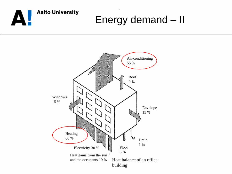
Energy demand – II

Heat balance of an office

building

Air-conditioning

55 %

Roof

9 %

Envelope

15 %

Drain

1 % Floor

5 %

Windows

15 %

Heating

60 %

Electricity 30 %

Heat gains from the sun

and the occupants 10 %

Need of heating

and cooling

Weather (climatic factors)

• variation and duration of outdoor

temperatures

• wind and precipitation

• snow cover and frost

• solar irradiation

Heating demand

• conduction through envelope (outer

walls, roof etc.) and floor

• ventilation, domestic hot water

• heat loads from solar, human and

other sources

• degree days

• design temperature

Cooling demand

• heat loads from solar, human and

other sources

• mass of the building

• overheating degree hours

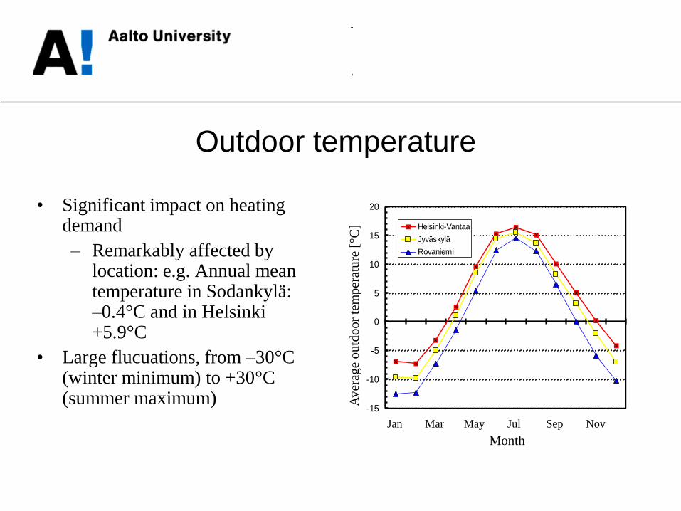
Outdoor temperature

• Significant impact on heating demand

– Remarkably affected by location: e.g. Annual mean temperature in Sodankylä: –0.4°C and in Helsinki +5.9°C

• Large flucuations, from –30°C (winter minimum) to +30°C (summer maximum)

-15

-10

-5

0

5

10

15

20

tammi maalis touko heinä syys marras

Kuukausi

Ke

sk

im. u

lko

läm

pö

tila

, °C

Helsinki-Vantaa

Jyväskylä

Rovaniemi

Av

erag

e o

utd

oor

tem

per

atu

re [

°C]

Month

Jan Mar May Jul Sep Nov

Diurnal (daily) temperature variation

• The highest temperature occurs at

some 2–3 hours after noon.

• The lowest temperature occurs

approximately at the time of

sunrise.

• In the darkest season (between

November and January) the

temperature variation does not

really follow the altitude of the

sun.

Ilm

an

lä

mp

öti

la

Aika

Auringonnousun aika

N. 15.00

Keskilämpötila

Outd

oo

r te

mper

atu

re

Mean temperature

Sunrise

Ca. 3 P.M.

Time

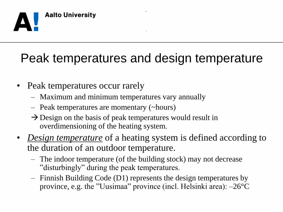
Peak temperatures and design temperature

• Peak temperatures occur rarely

– Maximum and minimum temperatures vary annually

– Peak temperatures are momentary (~hours)

Design on the basis of peak temperatures would result in overdimensioning of the heating system.

• Design temperature of a heating system is defined according to the duration of an outdoor temperature.

– The indoor temperature (of the building stock) may not decrease ”disturbingly” during the peak temperatures.

– Finnish Building Code (D1) represents the design temperatures by province, e.g. the ”Uusimaa” province (incl. Helsinki area): –26°C

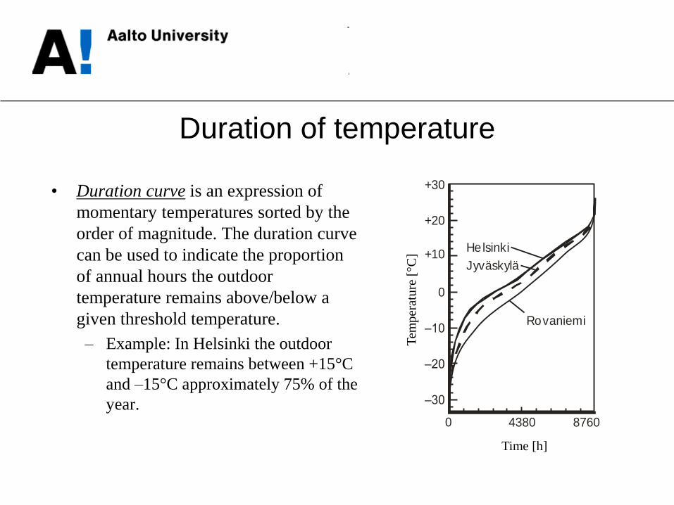
Duration of temperature

• Duration curve is an expression of

momentary temperatures sorted by the

order of magnitude. The duration curve

can be used to indicate the proportion

of annual hours the outdoor

temperature remains above/below a

given threshold temperature.

– Example: In Helsinki the outdoor

temperature remains between +15°C

and –15°C approximately 75% of the

year.

Tuntia vuodessa

Läm

pö

tila

, °C

–30

–20

–10

0

+10

+20

+30

0 8760

Helsinki

Jyväskylä

Rovaniemi

4380

Time [h]

Tem

per

atu

re [

°C]

Impact of the altitude (on the temperature)

• Significant variations possible

– affecting factors: ground heated by solar irradiation, thermal radiation from the ground to the space (ground temperature < air temperature)

– Shape of terrain

• Official height of temperature measurement: 2 m K

ork

eu

s m

aan

pin

nas

ta, m

Lämpötilaero, °C

0

5

10

15

20

25

–6 –4 –2 0 2 4 6 8–8

Päiv

ällä

Yöllä

Alt

itu

de

fro

m t

he

gro

un

d l

evel

[m

]

Temperature difference [°C]

Impact of shape of terrain (micro climate)

• Cold air accumulates into gorges, hollows, valleys and dingles

– Air layer close to the ground cools down during clear nights (because of radiation)

– Cool air flows towards valleys due to gravitation (”lakes of cold air”)

• Open waters (seas, lakes) significangly impact the micro climate

Matka, km

Ilm

an l

äm

pöti

la, °C

Ko

rke

us

, m

–30

–25

–20

–15

–10

–5

50

100

150

200

0 5 10 15

Maastonmuoto

Lämpöti la

Alt

itu

de

[m]

Distance [km]

Air

tem

per

atu

re [

°C]

Shape of

terrain

Temperature

Impact of wind

• There is no accurate method to evaluate the impact of wind, because

– Wind speed is measured from open areas (e.g. Airport) at the height of 10 m

– Wind speed varies significantly in the built environment and because of the shape of terrain, vegetation and proximity of open waters

• The average wind speed in

Finland is ca. 4 m/s

h

Tu

ule

n s

uh

teellin

en

no

peu

s

Etäisyys esteestä, h:n kerrannaisia

0

0,2

0,4

0,6

0,8

1,0

0 10 20

Pro

po

rtio

nal

win

d s

pee

d

Distance from an obstacle ×h

Humidity of air

• The moisture content (aka specific

humidity or humidity ratio) is the

mass of water vapour (v) in a

kilogram of dry air (a).

• At a given temperature, only a limited moisture content is allowed without condensation taking place. The relative humidity

(RH) indicates the used proportion of the capacity of the air to keep moisture at a given temperature.

The moisture content of outdoor air is low during cold weather (winter), but the relative humidity is high.

Kuukausikeskiarvot,

Helsinki-Vantaa

0

2

4

6

8

10

tammi huhti heinä loka

Ab

so

luu

ttin

en

ko

ste

us,

g/m

³0

20

40

60

80

100

Su

hte

ell

inen

ko

ste

us,

%

Mois

ture

co

nte

nt

[gv/m

3a]

Rel

ativ

e h

um

idit

y [

%]

Jan Apr Jul Oct

Montly average

Helsinki – Vantaa

Precipitation (rainfall)

• In Finland: evenly distributed precipitation throughout a year

• Annual precipitation: 400–700 mm

• Uniform frequency and intensity throughout the country

• Showers / flurries typically short S

ate

en

ran

kk

uu

s, m

m/m

in

Toistumisväli, vuotta1002 10 505 20

0

1

2

3

4

5Sateen kesto

1 min

2 min

5 min

10 min

20 min

60 min

3 min

Inte

nsi

ty o

f ra

infa

ll [

mm

/min

]

Recurrence interval [a]

Duration

Ground temperature, frost and blanket of snow

• Ground temperaure is

– A couple of degrees higher than the mean outdoor temperature

– Follows the outdoor temperature with a long delay (months)

• Snow blanket significantly affects ground frost:

– Ground covered by snow only freezes close to the surface (depth 30–50 cm)

– Ground frost depends on the soil: gravel freezes more deeply than clay

0

1

2

3

4

5

6

7

8

9

10

Syvy

ys m

aan

pin

nas

ta, m

Maan lämpötila, °C

181614121086420–2–4–6

Lumipeitteinenmaa

Paljasmaa

Ground temperature [°C]

Dep

th [

m]

Bare

ground

Ground

covered

by snow

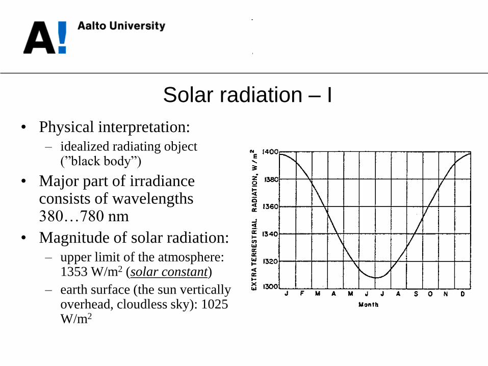
Solar radiation – I

• Physical interpretation:

– idealized radiating object (”black body”)

• Major part of irradiance consists of wavelengths 380…780 nm

• Magnitude of solar radiation:

– upper limit of the atmosphere: 1353 W/m2 (solar constant)

– earth surface (the sun vertically overhead, cloudless sky): 1025 W/m2

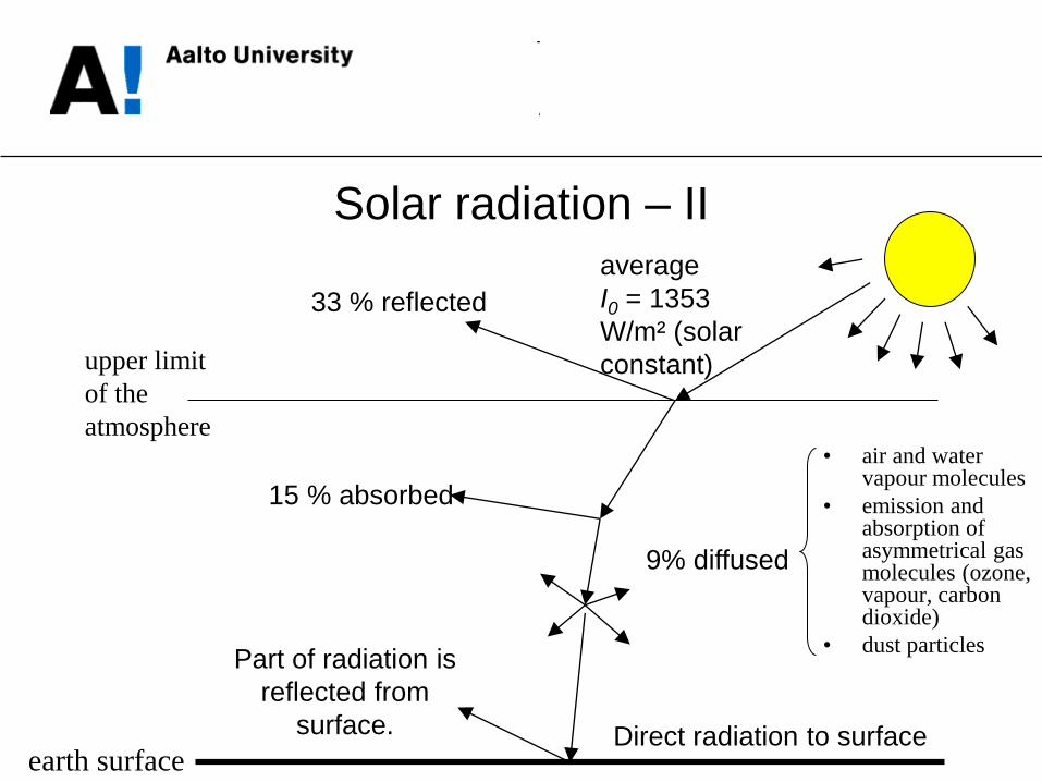
Solar radiation – II

average

I0 = 1353

W/m² (solar

constant)

33 % reflected

earth surface

upper limit

of the

atmosphere

15 % absorbed

9% diffused

Direct radiation to surface

Part of radiation is

reflected from

surface.

• air and water vapour molecules

• emission and absorption of asymmetrical gas molecules (ozone, vapour, carbon dioxide)

• dust particles

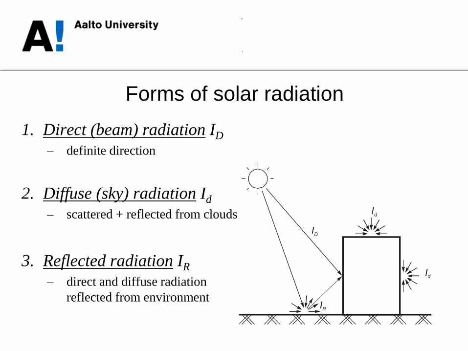
Forms of solar radiation

1. Direct (beam) radiation ID

– definite direction

2. Diffuse (sky) radiation Id

– scattered + reflected from clouds

3. Reflected radiation IR

– direct and diffuse radiation

reflected from environment

ID

IR

Id

Id

Annual solar irradiation

Horizontal plane: ca. 900 kWh/m2,a

• November to January: 19 kWh/m2 in total (diffuse radiation incl.)

• Summer: ca. 150 kWh/m2,kk

Vertical surfaces (rooms, windows):

• Southern wall (ca. 550 kWh/m2,a)

• Northern wall (ca. 230 kWh/m2a)

• Eastern and western wall: in winter the irradiation is shared evenly with the northern wall, in summer they receive more irradiation than the southern wall

Latitude

Annual

irradiation

[kWh/m2]

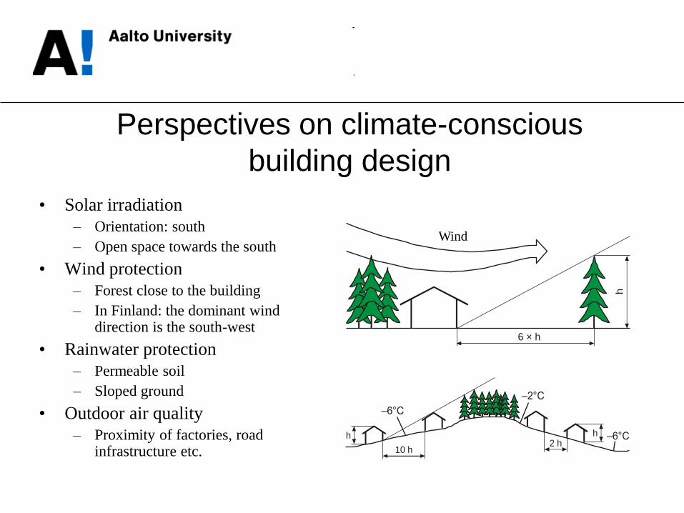
Perspectives on climate-conscious

building design

• Solar irradiation

– Orientation: south

– Open space towards the south

• Wind protection

– Forest close to the building

– In Finland: the dominant wind direction is the south-west

• Rainwater protection

– Permeable soil

– Sloped ground

• Outdoor air quality

– Proximity of factories, road infrastructure etc.

6 × h

h

Tuuli

10 h

–6°C

–2°C

–6°C2 h

hh

Wind

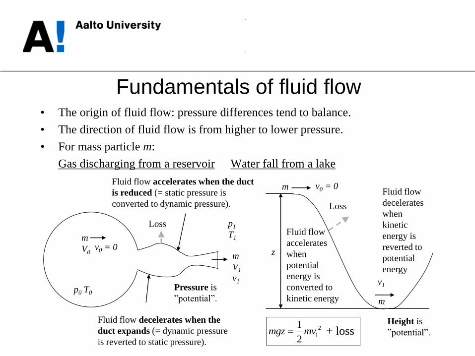
Fundamentals of fluid flow • The origin of fluid flow: pressure differences tend to balance.

• The direction of fluid flow is from higher to lower pressure.

• For mass particle m:

Gas discharging from a reservoir Water fall from a lake

m

V0 v0 = 0

p0 T0

m

V1

v1

p1

T1

Fluid flow decelerates when the

duct expands (= dynamic pressure

is reverted to static pressure).

Fluid flow accelerates when the duct

is reduced (= static pressure is

converted to dynamic pressure).

Pressure is

”potential”.

z

m v0 = 0

m

v1

Height is

”potential”.

Fluid flow

accelerates

when

potential

energy is

converted to

kinetic energy

Loss

2

1

1häviöt

2mgz mv

Fluid flow

decelerates

when

kinetic

energy is

reverted to

potential

energy

Loss

+ loss

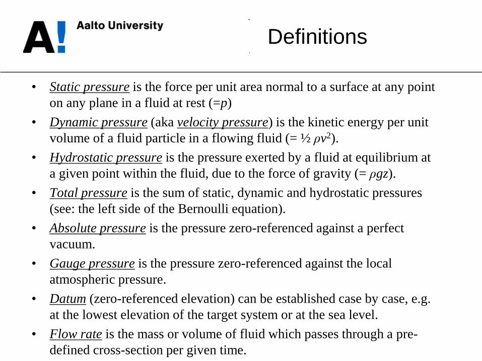
Definitions

• Static pressure is the force per unit area normal to a surface at any point

on any plane in a fluid at rest (=p)

• Dynamic pressure (aka velocity pressure) is the kinetic energy per unit

volume of a fluid particle in a flowing fluid (= ½ ρv2).

• Hydrostatic pressure is the pressure exerted by a fluid at equilibrium at

a given point within the fluid, due to the force of gravity (= ρgz).

• Total pressure is the sum of static, dynamic and hydrostatic pressures

(see: the left side of the Bernoulli equation).

• Absolute pressure is the pressure zero-referenced against a perfect

vacuum.

• Gauge pressure is the pressure zero-referenced against the local

atmospheric pressure.

• Datum (zero-referenced elevation) can be established case by case, e.g.

at the lowest elevation of the target system or at the sea level.

• Flow rate is the mass or volume of fluid which passes through a pre-

defined cross-section per given time.

Pressures

• Atmospheric pressure:

– Sea level: 101325 Pa

• Selected pressures in heating and piping technology:

– District heating (primary): +1.5 Mpa (15 bar) (max.)

– City water: +300 kPa

– Cold water distribution system: +200...250 kPa

– Pressure difference over a radiator valve: 2...4 kPa

– Pressure drop of a heat distribution network: > 10 kPa

Conservation laws

• ”...cannot be created or destroyed”

1. Conservation of mass

2. Conservation of energy

3. Conservation of momentum

Control

volume

Flow in = Flow out

Self-studying: Learn the governing principle for the

conservation of momentum and apply it to determine the force

caused by the change of direction of a fluid flow in a tube.

Conservation of mass

qm1

A1

v1

ρ1

qm2

A2

v2

ρ2

Cross sections 1 and 2

of a tube/pipe/duct Reduction

1 2 1 1 1 2 2 2m mq q Av A v

Continuity equation

[qm] = kg/s

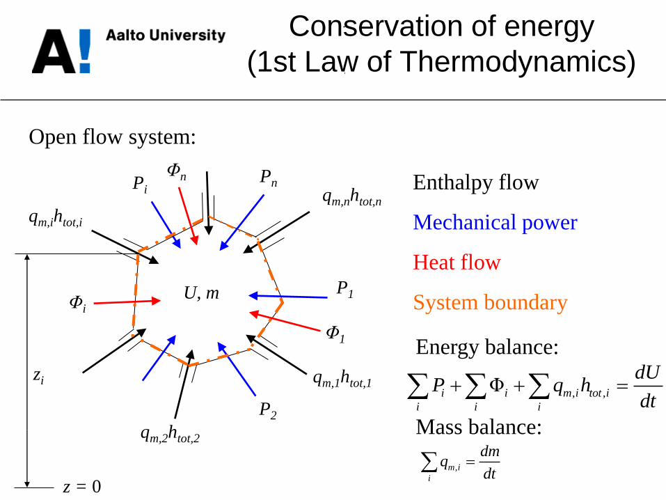
Conservation of energy

(1st Law of Thermodynamics)

Enthalpy flow

Mechanical power

Heat flow

System boundary

, ,Φi i m i tot i

i i i

dUP q h

dt

Energy balance:

Mass balance:

,m i

i

dmq

dt

qm,1htot,1

qm,nhtot,n

qm,ihtot,i

qm,2htot,2

P1

P2

Pn Pi

Φi

Φ1

Φn

zi

z = 0

U, m

Open flow system:

Energy content of fluid

flow (enthalpy)

• Total specific enthalpy

where cp = specific heat capacity of the fluid at constant pressure

cV = specific heat capacity of the fluid at constant volume

p = static pressure of the fluid at the system boundary

ρ = density of the fluid

t = temperature of the fluid (zero-point of the temperature scale is an agreed reference temperature e.g. 0°C)

hm = chemical specific energy, ”enthalpy of formation” (e.g. LHV or HHV)

v = fluid velocity

g= gravitational acceleration

z = altitude (zero-point optional case by case)

In the equation of total specific enthalpy [J/kg], the relevant energy forms are included. The equation above does not contain surface energy (in HVAC applications, the surface energy can be neglected since it does not significantly affect the accuracy of the results).

2 21 1

2 2tot p m V m

ph c t h v gz c t h v gz

Bernoulli equation – I

A1

v1

htot

ρ

z1

t

Reduction

A2

v2

htot

ρ

z2

t

Assumptions:

• incompressible flow (ρ1 = ρ2 = ρ)

• isothermal system (T1 = T2 = T)

• no friction

• continuity:

p1 p2

Cross sections 1 and 2

of a tube/pipe/duct

221121 vAvAqq VV

Bernoulli equation – II

• Energy conservation: total specific enthalpy remains

• By reducing (adiabatic fluid) the term cvt, considering that

hm = 0 and multiplying both sides of the equation by density:

This is the Bernoulli equation, which is analogous to the conservation of energy

(e.g. potential and kinetic energy).

2 21 2

1 1 2 2

1 1

2 2V m V m

p pc t h v gz c t h v gz

2 2

1 1 1 2 2 2

1 1

2 2totp v gz p v gz p

In words:

Total pressure (ptot) =

static pressure

+ dynamic pressure

+ hydrostatic pressure

Self-studying: Learn how to derive the Bernoulli equation through

integrating Newton's Second Law of Motion (i.e. Euler Equation).

s

m9,9 m 5

s

m 81.92

2

200

constant2

constant2

2

1221

2 State

2

22

1 State

11

2

111

2

111

gzvpp

g

v

g

p

g

pz

g

v

g

pz

vgzp

Calculate the fluid velocity at state 2.

Example

10cm

State 1

State 2

z1 = 5 m

Assumption: v1 ~ 0

z2 = 0 m

Assumption: no pressure loss

fppvgzpvgzp 2

222

2

1112

1

2

1

For straight pipe:

Pipe components (crosses, elbows, bends etc.): 2

2

1vKp

For rectangular tubes Dh is calculated from

)(2

44

ba

ab

P

ADh

z 1

z 2

ρ = const p

v 1

1

p

v 2

2

A

When pressure loss is accounted, the law of energy

conservation is applied as follows:

Pressure loss (head)

2

2

1v

D

Lfp

h

f

Friction loss

Hydraulic diameter

loss terms

Minor loss

Friction factor

• Friction factor f:

• Reynolds number:

2

9.0Re

7.5

7.3

/ln

325.1

hDf

hvD

Re

Re

64

:3000) (Re flowlaminar For

f

[m] pipe theof roughness

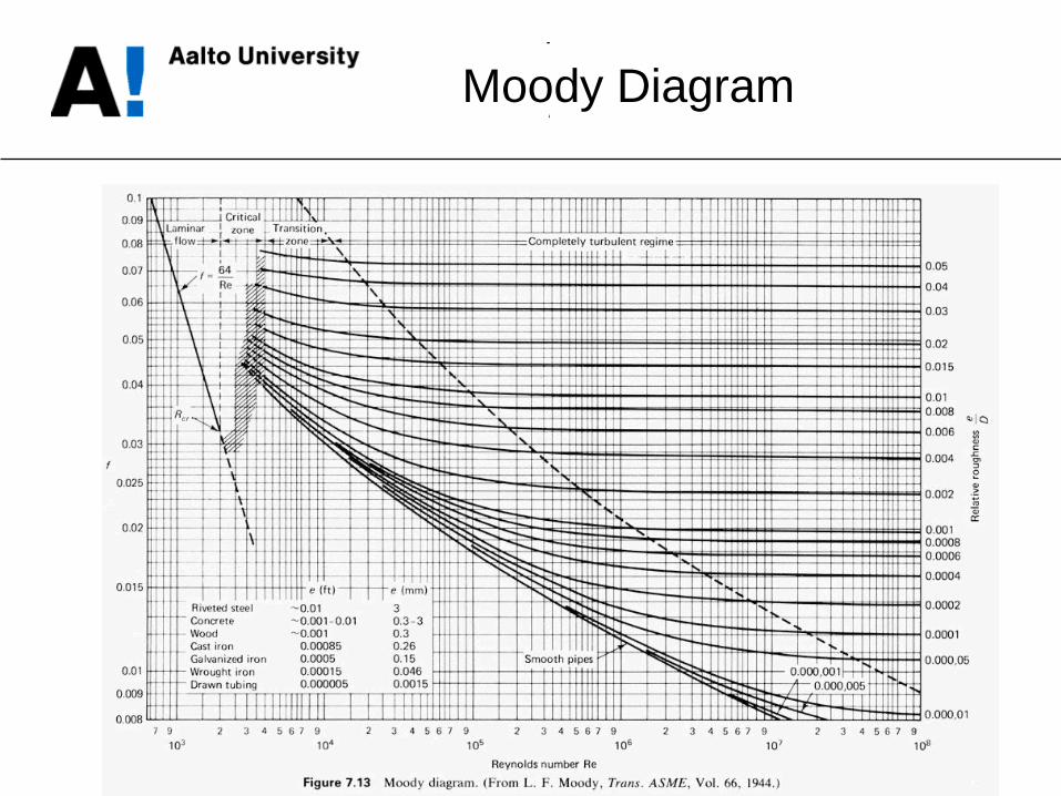
Moody Diagram

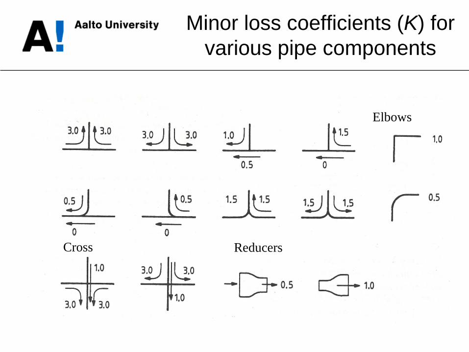
Minor loss coefficients (K) for

various pipe components

Cross Reducers

Elbows

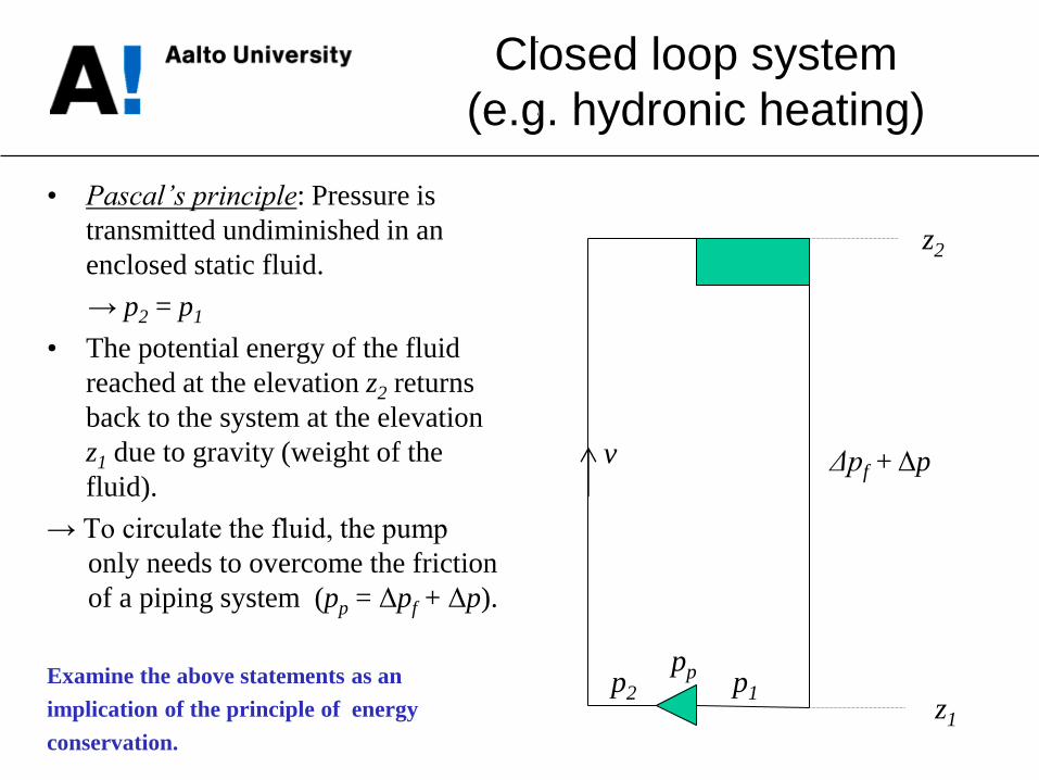
Closed loop system

(e.g. hydronic heating)

• Pascal’s principle: Pressure is

transmitted undiminished in an

enclosed static fluid.

→ p2 = p1

• The potential energy of the fluid

reached at the elevation z2 returns

back to the system at the elevation

z1 due to gravity (weight of the

fluid).

→ To circulate the fluid, the pump

only needs to overcome the friction

of a piping system (pp = Δpf + Δp).

Examine the above statements as an

implication of the principle of energy

conservation.

z2

z1

pp

Δpf + Δp

p2 p1

v

Example

City water is delivered at 300 kPa (3 bar) and the pressure

loss of the water distribution system is 100 kPa.

Is the pressure (300 kPa) sufficient to distribute water at the

volumetric flow rate of 0.2 L/s to a tap (inside diameter 10

mm) elevated at 20 m from the city water interface (inside

diameter 16 mm)? (Inversely: Do we need a pump to deliver

the requested water flow rate?)

The density of water ρ = 1000 kg/m3 and the standard gravity

g = 9.81 m/s2

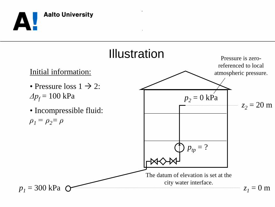
Illustration

p1 = 300 kPa

Initial information:

• Pressure loss 1 2:

Δpf = 100 kPa

• Incompressible fluid:

ρ1 = ρ2= ρ

z1 = 0 m

z2 = 20 m

p2 = 0 kPa

ptp = ?

The datum of elevation is set at the

city water interface.

Pressure is zero-

referenced to local

atmospheric pressure.

Solution – I

1. Energy conservation:

Note: how to

substitute the

pump pressure in

the energy

equation?

12

2

1

2

22

1 ppgzvvp ftp

ftp pgzvppgzvp 2

2

221

2

112

1

2

1

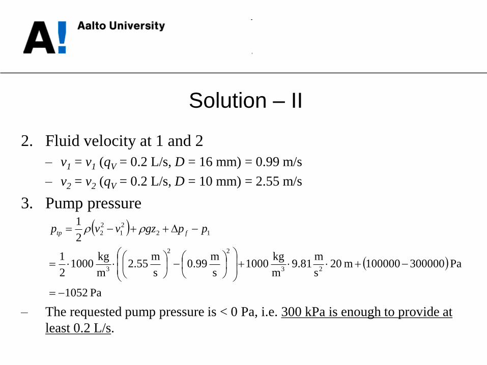
Solution – II

2. Fluid velocity at 1 and 2

– v1 = v1 (qV = 0.2 L/s, D = 16 mm) = 0.99 m/s

– v2 = v2 (qV = 0.2 L/s, D = 10 mm) = 2.55 m/s

3. Pump pressure

– The requested pump pressure is < 0 Pa, i.e. 300 kPa is enough to provide at

least 0.2 L/s.

Pa 1052

Pa 300000100000m 20s

m 81.9

m

kg 1000

s

m 99.0

s

m 55.2

m

kg 1000

2

1

2

1

23

22

3

12

2

1

2

2

ppgzvvp ftp

Example

Calculate the friction loss per 1 m of a straight air duct

(diameter 500 mm, roughness 0.15 mm) at volumetric flow

rates 1, 2 and 3 m3/s. The air temperature is 300 K.

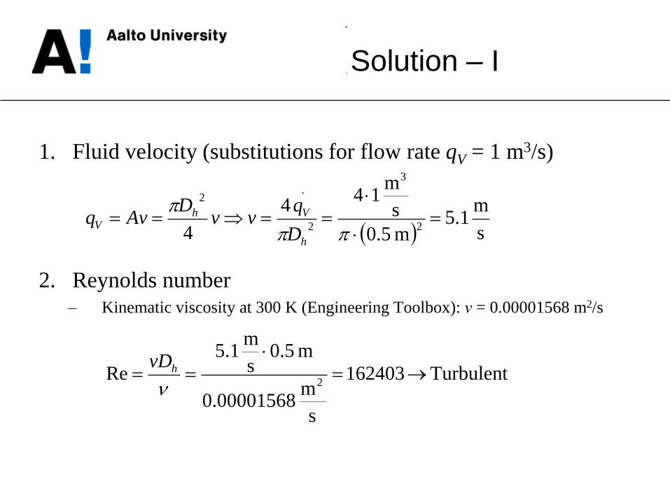
Solution – I

1. Fluid velocity (substitutions for flow rate qV = 1 m3/s)

2. Reynolds number

– Kinematic viscosity at 300 K (Engineering Toolbox): ν = 0.00001568 m2/s

s

m 1.5

m 5.0

s

m 14

4

42

3

2

.2

h

VhV

D

qvv

DAvq

Turbulent 162403

s

m 00001568.0

m 5.0s

m 1.5

Re2

hvD

Solution – II

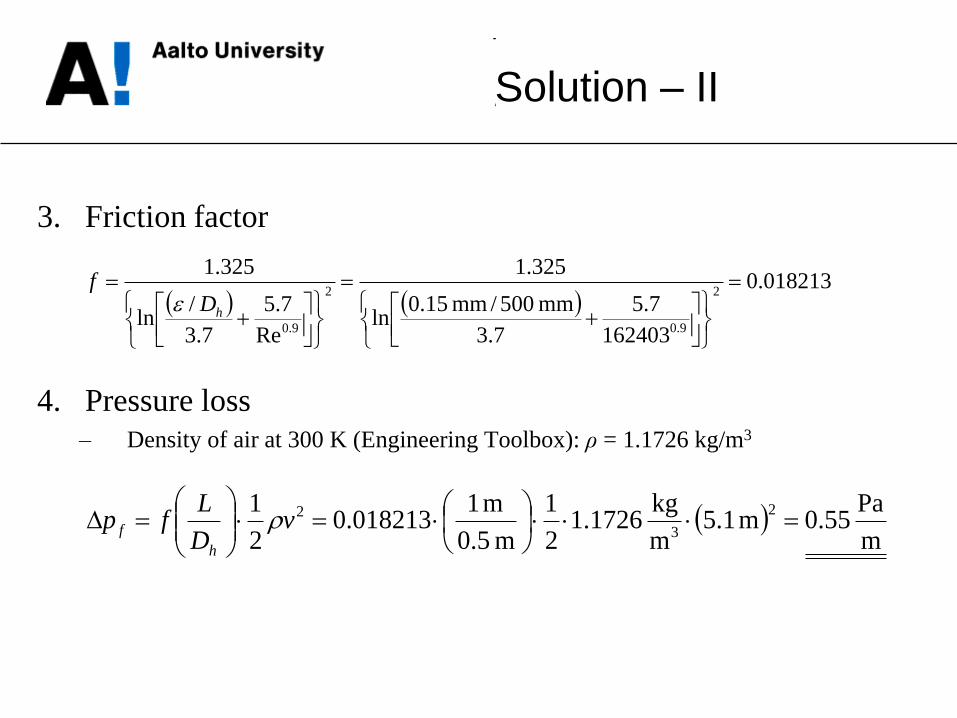
3. Friction factor

4. Pressure loss

– Density of air at 300 K (Engineering Toolbox): ρ = 1.1726 kg/m3

018213.0

162403

7.5

7.3

mm 500/mm 15.0ln

325.1

Re

7.5

7.3

/ln

325.12

9.0

2

9.0

hDf

m

Pa 55.0m 1.5

m

kg 1726.1

2

1

m 5.0

m 1018213.0

2

1 2

3

2

v

D

Lfp

h

f

Summary of results

[m3/s] v [m/s] Re Quality f Δpf [Pa/m]

1 5.1 162403 Turbulent 0.018 0.55

2 10.2 324806 Turbulent 0.017 2.06

3 15.3 487209 Turbulent 0.016 4.49

Vq

Introduction to heat transfer

1 CONDUCTION

• Transfer of kinetic energy of particles

• Solid materials, fluids and gases

2 CONVECTION

• Heat transfer with the movement of fluid

• Forced or free (natural)

• Takes place between a solid surface and a fluid

3 RADIATION

• Electromagnetic wave motion

• All the solid bodies emit radiation

Hot Cold

v

T

Boundary layers

Tmax

vmax

• The origin of heat transfer: temperature differences

tend to balance.

• The direction of heat flow (and heat flux, i.e. heat

flow per m2) is from higher to lower temperature.

• Three (3) forms of heat transfer:

• Governing equation: The Fourier equation

where q = heat flux, W/m2

λ = thermal conductivity, W/mK

T = temperature, K

s = insulation thickness, m

Φ = heat flow, W

A = surface area, m2

• Implementation (for the case on the right):

where = thermal resistance, m2K/W

R

T

s

TTTT

sq

dTqdxdx

dT

x

Tq

s T

T

2121

0

)(

2

1

T2

T1

x = 0 x = s

λ

Inn

er s

urf

ace

Fundamentals of conduction

As

Tq

Assumption: one-dimensional conduction

through surface (wall etc.)

Self-studying: Formulate the heat conduction

equation for a three-dimensional control volume.

sR

Thickness,

cm

Heat flux,

W/m2

5 37

10 19

15 12.5

20 9.4

25 7.5

30 6.3

0

10

20

30

40

5 10 15 20 25 30

q, W/m2

s, cm

Example: Impact of

insulation thickness

ΔT = 47 K

λ = 0.04 W/mK

A mathematical justification to

avoid too thick an insulation.

)expression (general

right) on the (wall

1

11

41

433221

n

i i

i

n

c

c

b

b

a

a

c

c

b

b

a

a

s

TTq

sss

TTq

TTs

TTs

TTs

q

Implementation:

Conduction through wall

element (”sandwich”)

)()(:and res temperatuSurface 41

1

1341

1

1232 TTs

ss

TTTTs

s

TTTTn

i i

i

b

b

a

a

n

i i

i

a

a

T2

T1

λa

T3

T4 λb

λc

sa sb sc

q q

The temperature difference over the wall (T1 – T4) is apportioned according to the proportion of

thermal resistances (i.e. the largest thermal resistance → the largest temperature difference etc.):

Heat flux through wall remains the same through each layer (stationary conditions):

RT ~

Insulation

Example

T1 = +20 °C

si = 10 12.5 10 cm

λi = 0.9 0.04 0.5 W/mK

T4 = –20 °C

Concrete Wool Brick

T2 = ?

T3 = ? Calculate the heat flux and the

surface temperatures T2 and T3

for the wall on the right.

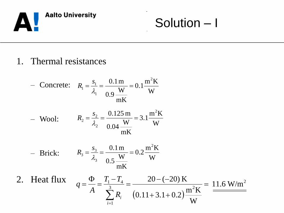
2

23

1

41 W/m6.11

W

Km 2.01.311.0

K )20(20

i

iR

TT

Aq

Solution – I

1. Thermal resistances

– Concrete:

– Wool:

– Brick:

2. Heat flux

W

Km1.0

mK

W 9.0

m 1.0 2

1

11

sR

W

Km1.3

mK

W 04.0

m 125.0 2

2

22

sR

W

Km2.0

mK

W 5.0

m 1.0 2

3

33

sR

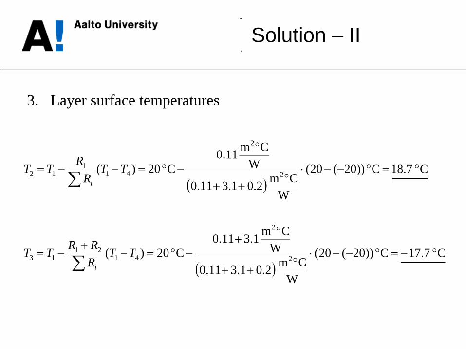
C7.17C ))20(20(

W

Cm 2.01.311.0

W

Cm 1.311.0

C 20)(

C7.18C ))20(20(

W

Cm 2.01.311.0

W

Cm 11.0

C 20)(

2

2

4121

13

2

2

411

12

TTR

RRTT

TTR

RTT

i

i

3. Layer surface temperatures

Solution – II

Fundamentals of convection

• Where there is a temperature difference between a fluid

and solid surface, convective heat transfer to/from

surface takes place.

• Types of convection: • free (natural): fluid flow is created by density

differences caused by temperature differences

• forced: fluid flow is created by external force (e.g. fan,

ventilator etc.)

• Governing equation:

where Φ = heat flow, W

α = heat transfer coefficient, W/m2K

T1 = surface temperature, K or °C

T2 = temperature of free fluid, K or °C

TTTq 21

Fluid velocity

Temperature

difference

dT dx

Free convection from a

warm surface (T1 >T2)

T

T

2

1

lkrσ

x

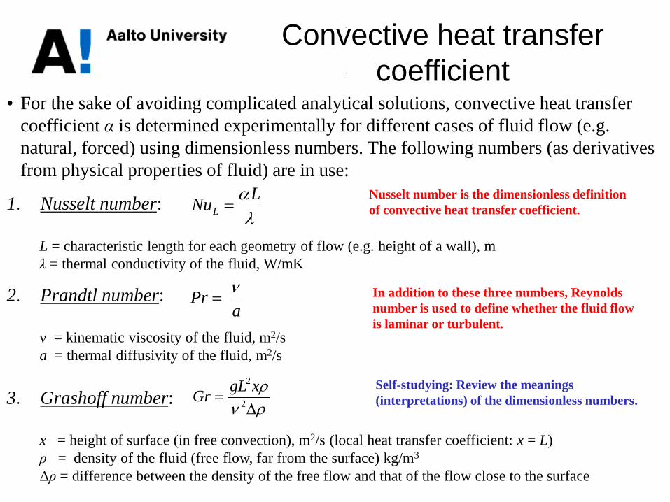
• For the sake of avoiding complicated analytical solutions, convective heat transfer

coefficient α is determined experimentally for different cases of fluid flow (e.g.

natural, forced) using dimensionless numbers. The following numbers (as derivatives

from physical properties of fluid) are in use:

1. Nusselt number:

L = characteristic length for each geometry of flow (e.g. height of a wall), m

λ = thermal conductivity of the fluid, W/mK

2. Prandtl number:

ν = kinematic viscosity of the fluid, m2/s

a = thermal diffusivity of the fluid, m2/s

3. Grashoff number:

x = height of surface (in free convection), m2/s (local heat transfer coefficient: x = L)

ρ = density of the fluid (free flow, far from the surface) kg/m3

Δρ = difference between the density of the free flow and that of the flow close to the surface

LNuL

aPr

Convective heat transfer

coefficient

2

2xgLGr

Self-studying: Review the meanings

(interpretations) of the dimensionless numbers.

Nusselt number is the dimensionless definition

of convective heat transfer coefficient.

In addition to these three numbers, Reynolds

number is used to define whether the fluid flow

is laminar or turbulent.

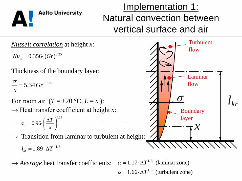
Nusselt correlation at height x:

Thickness of the boundary layer:

For room air (T = +20 °C, L = x ):

→ Heat transfer coefficient at height x:

→ Transition from laminar to turbulent at height:

→ Average heat transfer coefficients:

lkrσ

x

Implementation 1:

Natural convection between

vertical surface and air

25.0

96.0

x

Tx

3/189.1 Tlkr

zone) (turbulent 66.1

zone)(laminar 17.1

3/1

3/1

T

T

25.0)(356.0 GrNux

25.034.5 Grx

Turbulent

flow

Laminar

flow

Boundary

layer

Example

lkrσ

x

a) Derive the convective heat transfer

coefficient at height x (αx) from

the Nusselt number and Nusselt

correlation for air at T = 20°C.

b) Calculate the thickness of the

boundary layer (σ) and the

position of the transition zone (lkr)

at x = 1 m and ΔT = 2°C.

c) Sketch a graph for the average

heat transfer coefficient of the

laminar zone for ΔT = 0...20°C.

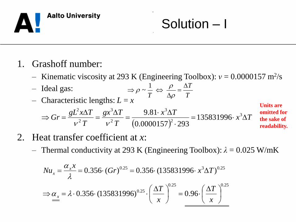
Solution – I

1. Grashoff number:

– Kinematic viscosity at 293 K (Engineering Toolbox): ν = 0.0000157 m2/s

– Ideal gas:

– Characteristic lengths: L = x

2. Heat transfer coefficient at x:

– Thermal conductivity at 293 K (Engineering Toolbox): λ = 0.025 W/mK

T

T

T

1~

Tx

Tx

T

Tgx

T

TxgLGr

3

2

3

2

3

2

2

1358319962930000157.0

81.9

Units are

omitted for

the sake of

readability.

25.025.0

25.0

25.0325.0

96.0)135831996(356.0

)135831996(356.0)(356.0

x

T

x

T

TxGrx

Nu

x

xx

3. Grashoff number:

– Air at 293 K: ν = 0.0000157 m2/s

– We choose the characteristic length: L = x = 1 m

– At ΔT = 2°C (K):

4. Thickness of the boundary layer:

5. Position of the transition zone:

8

22

3

2

2

3

106.2

K 293)s

m 0000157.0(

K2m 1s

m 81.9

T

TgxGr

Solution – II

cm4m04.0)106.2(34.534.5 25,0825.0 Gr

m 5.1K 289.189.13/13/1

Tlkr

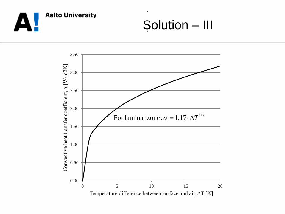
Solution – III

0.00

0.50

1.00

1.50

2.00

2.50

3.00

3.50

0 5 10 15 20

Co

nv

ecti

ve

hea

t tr

ansf

er c

oef

fici

ent,

α [

W/m

2K

]

Temperature difference between surface and air, ΔT [K]

3/117.1:zonelaminar For T

The convective heat transfer from

horizontal surface such as warm floor

or cold ceiling is more efficient than

that from a vertical surface.

Average heat transfer coefficient:

Example: Warm floor

3/126.2 T

ΔT 5 K 3.84 W/m2K

ΔT 20 K 6.07 W/m2K

Implementation 2:

Natural convection between

horizontal surface and air

Average heat transfer coefficient:

Example:

T1 = 40°C, T2 = 20°C, D = 15 mm

T1

T2

Implementation 3:

Natural convection between

tube and air

K W/m3.7m 015.0K 293

K 200.5 2

4

4

2

210.5DT

TT

Nusselt correlation:

For rectangle:

For gap:

Average heat transfer coefficients (v = fluid velocity, m/s):

h

D

vDRePrReNu where,023.0 33.08.0

)(2

44

ba

ab

P

ADh

dDh 2

a

b

d

K) W/m0.7 (default 0.7 : windbreakOuter wall

K) W/m1.11(default 1.11 :ndagainst wi Outer wall

K) W/m6.10(default 2.44.6 :roomin Surfaces

236.0

251.0

2

v

v

v

Implementation 4:

Forced convection

Dh

Temperature distribution through wall element

Ti

To

small large R

large T

small , small R, small T

Convection Convection Conduction

T1

T4

T2

T3

Internal temperature Ti > External temperature To

Thermal resistance of

the insulation (R) is

conclusive.

q

1

sR

sR

q

Insulation

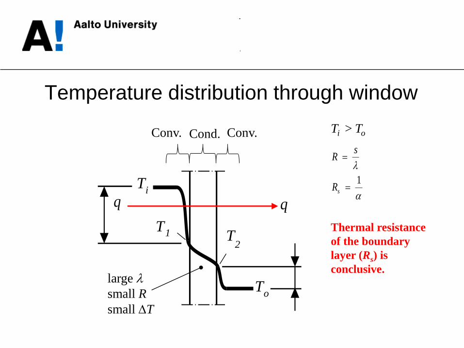
Temperature distribution through window

T

T T

T

i

1 2

o

Ti > To

Thermal resistance

of the boundary

layer (Rs) is

conclusive.

Conv. Conv. Cond.

qq

1

sR

sR

large small R

small T

How to calculate the

structure temperatures?

Ti

To

– + T1

i T4

o

T2

T3

so

o

si

i

R

TT

R

TT

R

TT

R

TT

R

TTq

4

3

43

2

32

1

211

oi i

i

i

i

so

i

isi

si

oi

i

sRRR

R

TT

TT

11

1

E.g.3

1

3

1

1

1

11

sR

i

siR

1

2

22

sR

3

33

sR

o

soR

1

Heat flux through wall remains the same through each layer (stationary conditions):

Rsi is known as

internal surface resistance.

Rso is known as

external surface resistance.

Total heat transfer coefficient aka thermal

transmittance aka U-value [W/m2K]:

Specific heat transfer coefficient aka

conductance [W/K]:

where A = area of the wall [m2]

Heat flow through wall [W]:

so

n

i

isi RRR

U

1

1

A

RRR

UAGn

i

soisi

1

1

U-value and conductance

Ti

Thermal resistances

Rsi, R1…Ri…Rn, Rso

oi TTUAqA

To

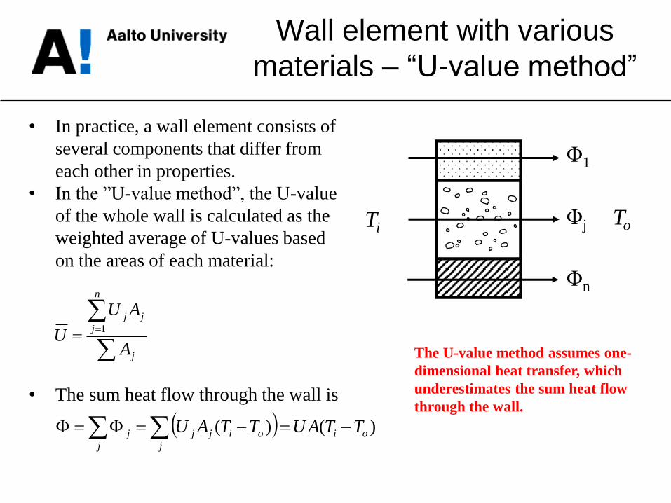
• In practice, a wall element consists of

several components that differ from

each other in properties.

• In the ”U-value method”, the U-value

of the whole wall is calculated as the

weighted average of U-values based

on the areas of each material:

• The sum heat flow through the wall is

Wall element with various

materials – “U-value method”

)()( oi

j

oijj

j

j TTAUTTAU

j

n

j

jj

A

AU

U1

The U-value method assumes one-

dimensional heat transfer, which

underestimates the sum heat flow

through the wall.

Ti To

Φ1

Φj

Φn

• In the ”Standard method” (based on the

Finnish Building Code C4), the λ-value of

a wall structure consisting of various

materials is calculated as the weighted

average of λ-values based on the areas of

each material:

• The total thermal resistance of the wall is

• The method assumes the temperature

between each layer (a, b, c) is constant

throughout the area, which allows new

layers to be easily added.

Wall element with various

materials – “Standard method”

b

bbb

sR

AAA

AAA

;

321

332211

so

c

aj

jsi RRRR

Rsi Rso

R1

1

R2

2

R3

3

sa sb sc

Ra Rb Rc

A1

A2

A3

A

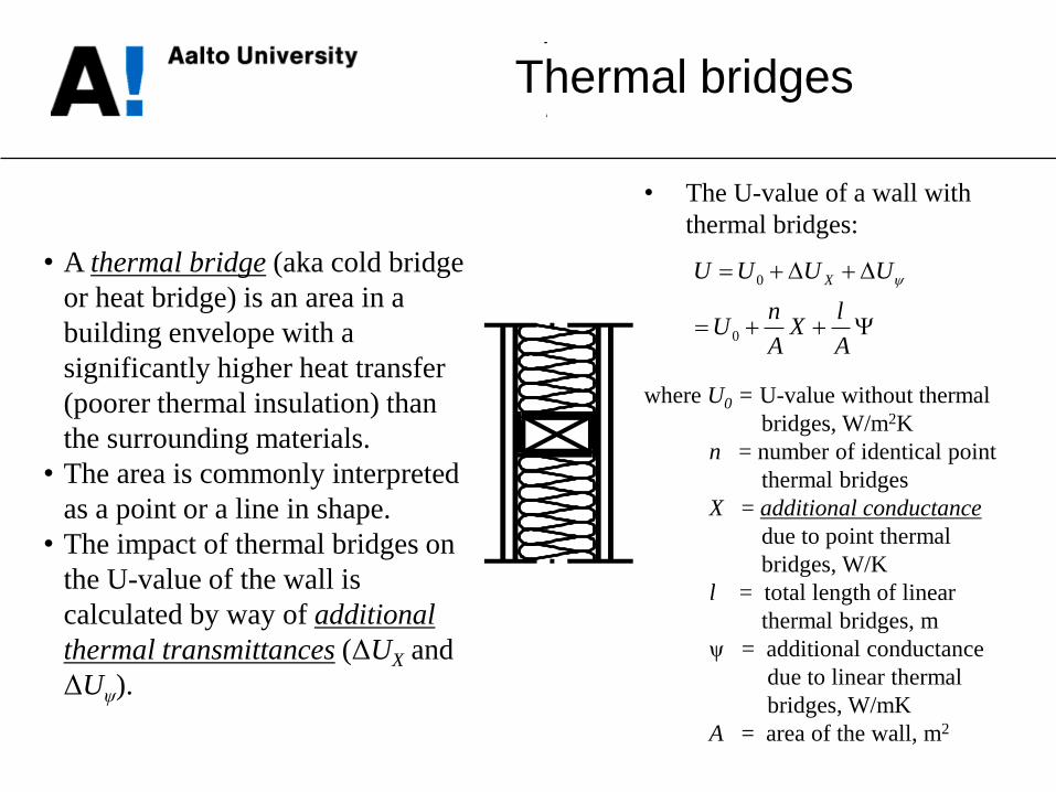
• The U-value of a wall with

thermal bridges:

where U0 = U-value without thermal

bridges, W/m2K

n = number of identical point

thermal bridges

X = additional conductance

due to point thermal

bridges, W/K

l = total length of linear

thermal bridges, m

ψ = additional conductance

due to linear thermal

bridges, W/mK

A = area of the wall, m2

Thermal bridges

• A thermal bridge (aka cold bridge

or heat bridge) is an area in a

building envelope with a

significantly higher heat transfer

(poorer thermal insulation) than

the surrounding materials.

• The area is commonly interpreted

as a point or a line in shape.

• The impact of thermal bridges on

the U-value of the wall is

calculated by way of additional

thermal transmittances (ΔUX and

ΔUψ).

A

lX

A

nU

UUUU X

0

0

Additional conductances for

linear thermal bridges

ψ = 0.35…0.57 W/mK

ψ = 0.002 W/mK

ψ = 0.12…0.17 W/mK

ψ = 0.02…0.03 W/mK

ψ = 0.6…0.8 W/mK

ψ = 0.1…0.5 W/mK

Fundamentals of

thermal radiation

• Thermal radiation is electromagnetic radiation emitted by a body or a surface on the basis of its temperature, not depending on the state of its surroundings.

• Radiant heat flux (aka radiance) [W/m2] of a black body (i.e. idealized physical body that absorbs all incident electromagnetic radiation) is calculated from

where σ = Stefan-Boltzmann constant (5.67·10-8 W/m2K4)

• In practice (realistic surface i) the radiance

is calculated from where i = emissivity of surface i [-] Fi = view factor of surface i (i.e. fraction of the surroundings the surface i represents) [-]

4TMm

miii M F M

Wavelength, µm

Sp

ectr

al r

adia

nce

, W

/m2, μ

m

0

10 2

10 4

10 6

10 8

4 8 12 16 20 24

λ T = 2898 µmK max

Visible light:

0.38 … 0.78 µm

Blue…Red

11

Fn

i

i

• Surfaces visible to each other receive (absorb and reflect) thermal radiation they emit

• Net heat transfer between two surfaces depends on surface temperatures, emissivities and their position with respect to each other as follows:

• Net heat transfer can be also expressed as

where αr = radiative heat transfer coefficient, W/m2K

• For parallel, infinite surfaces, αr can be defined as

• When surface 2 is large in comparison with surface 1:

2 missä 21 TT

T

)( 212112 TTqqq r

2 ;4 21

3 TTTTr

Net heat transfer

q = q1 – q2

T1

q1

q2

T2

111

21

4

2

4

112

TT

q

Radiative heat

transfer coefficient

ε1 ε2

111

4

21

3

Tr

• Total heat transfer to/from a surface entails both convection (c) and radiation (r):

q = qc + qr

• The share of convection in the total heat transfer is calculated from

qc = c (Ts,i –Ta )

where c = convective heat transfer coefficient

Ts,i = temperature of surface i

Ta = air temperature

• The share of convection in the total heat transfer is calculated from

qr = r (Ts,i –Ts )

where r = radiative heat transfer coefficient

Ts,i = temperature of surface i

Ts = temperature of other surfaces (excluding i) (assumption: they have equal temperature)

• The total heat transfer coefficient is

• With an acceptable accuracy can be stated: q = (c + r )(Ts,i –Ta ) = (Ts,i –Ta )

Total heat transfer

coefficient

r

ais

sis

cTT

TT

,

, Ts commonly

unknown

Example

Km

W0.9

193.0

1

93.0

1

K 358Km

W1067.54

111

4

K 3582

K293423

2

3

42

8

21

3

r

T

T

The graph summarizes the total

heat transfer coefficient of a

horizontal tube, indicating the

share of convective and radiative

heat transfer. The data are valid

for Ta = 20°C (293 K). The

emissivities for both the tube (1)

and its surroundings (2) can be

assumed 1 = 2 = 0.93.

Show through calculation the

radiative heat transfer coefficient

(r) at the surface temperature of 150°C (423 K).

Solution: