Journal of Geophysical Research: Space Physics

BRIEF REPORT10.1002/2013JA019663

Key Points:• Energetic electron distribution

during heating experiment deducedfrom airglow

• Inferred electron energy spectrumsufficient to induce ionization

• Results depend on inhomogeneity ofairglow, which is filamentary

Correspondence to:D. L. Hysell,dlh37@cornell.edu

Citation:Hysell, D. L., R. J. Miceli, E. A. Kendall,N. M. Schlatter, R. H. Varney, B. J.Watkins, T. R. Pedersen, P. A. Bernhardt,and J. D. Huba (2014), Heater-inducedionization inferred from spectro-metric airglow measurements,J. Geophys. Res. SpacePhysics, 119, 2038–2045,doi:10.1002/2013JA019663.

Received 27 NOV 2013

Accepted 4 FEB 2014

Accepted article online 10 FEB 2014

Published online 1 MAR 2014

Heater-induced ionization inferred from spectrometricairglow measurementsD. L. Hysell1, R. J. Miceli1, E. A. Kendall2, N. M. Schlatter3, R. H. Varney4, B. J. Watkins5, T. R. Pedersen6,P. A. Bernhardt7, and J. D. Huba7

1Earth and Atmospheric Sciences, Cornell University, Ithaca, New York, USA, 2SRI International, Menlo Park, California,USA, 3School of Electrical Engineering, Royal Institute of Technology Stockholm, Sweden, 4HAO NCAR, Boulder, Colorado,USA, 5Geophysical Institute, University of Alaska Fairbanks, Fairbanks, Alaska, USA, 6Space Vehicles Directorate, Air ForceResearch Laboratory, Albuquerque, New Mexico, USA, 7Plasma Physics Division, Naval Research Laboratory, Washington,District of Columbia, USA

Abstract Spectrographic airglow measurements were made during an ionospheric modificationexperiment at High Frequency Active Auroral Research Program on 12 March 2013. Artificial airglowenhancements at 427.8, 557.7, 630.0, 777.4, and 844.6 nm were observed. On the basis of these emissionsand using a methodology based on the method of Backus and Gilbert (1968, 1970), we estimate thesuprathermal electron population and the subsequent equilibrium electron density profile, includingcontributions from electron impact ionization. We find that the airglow is consistent with heater-inducedionization in view of the spatial intermittency of the airglow.

1. Introduction

The production of enhanced optical airglow was one of the first phenomena to be associated with iono-spheric modifications by high-power HF waves [Biondi et al., 1970; Haslett and Megill, 1974; Adeishvili et al.,1978] and continues to be a focus of research and attention (see review by Gurevich [2007]). While it was ini-tially believed that the enhancements could be explained in terms of heating and the enhancement of thetail of the thermal electron population [Mantas, 1994; Mantas and Carlson, 1996], the measured ratios of redand green line emissions and the appearance of optical emissions with high-energy thresholds signaled thepresence of a nonthermal component of the electron energy distribution [Bernhardt et al., 1989; Gustavssonet al., 2001, 2003; Djuth et al., 2005; Gustavsson et al., 2005]. Observations of the O+ 732–733 nm emissionduring heating experiments consistent with electron impact ionization also supported this proposition[Mutiso et al., 2008].

Recently, Pedersen et al. [2010] reported the creation of a layer of ionization over High Frequency ActiveAuroral Research Program (HAARP) sufficiently dense to support further ionospheric interactions. The layerwas produced initially at 220 km altitude using full power O-mode HF heating in the direction of magneticzenith and at a pump frequency very close to the second electron gyroharmonic frequency at that altitude.Once produced, the layer descended to a terminal altitude of about 150 km. Layer production was accom-panied by intense optical emissions which were filamentary and highly intermittent spatially. The authors ofthe study posited that the “layer” was likely spatially structured itself, with most of the enhanced ionizationcoming from the brightest kilometer-scale optical filaments.

The proposition of artificial ionization through ionospheric heating is also supported by other, more directmeasurements. Rose et al. [1985] published in situ measurements from rocket experiments showing electronenergies up to 10 eV. Carlson et al. [1982] published incoherent scatter plasma line measurements estab-lishing suprathermal electron spectra reaching at least 20 eV. It was this latter, quantitative confirmation ofelectrons exceeding the ionization potentials for O, O2, and N2 that enabled the prediction that a significantartificial ionosphere could be produced once HF facilities approached 1 GW ERP (effective radiated power)[Carlson, 1993]. It was nearly two decades before this prediction could be tested at HAARP and EuropeanIncoherent Scatter. Experiments at HAARP had sufficient supporting optical data to verify the presence ofelectron excitation above the N+

2 ionization threshold [Pedersen et al., 2009].

Assessing the possibility of heater-induced ionization requires an estimate of the electron energy distribu-tion which, in principle, can be formulated on the basis of airglow measurements at a number of spectral

HYSELL ET AL. ©2014. American Geophysical Union. All Rights Reserved. 2038

Journal of Geophysical Research: Space Physics 10.1002/2013JA019663

lines. On the basis of emissions at 630.0, 557.7, 844.6, and 427.8 nm together with other information derivedfrom incoherent scatter radar, Gustavsson et al. [2005] estimated the electron energy distribution between1 and nearly 100 eV. The problem can be regarded as an underdetermined or mixed-determined inverseproblem, amenable to solution through a number of different methodologies [Menke, 1984; Tarantola, 1987;Aster et al., 2005]. Gustavsson et al. [2005] expressed the energy distribution as a piecewise-continuous func-tion parameterized by a small number of constants and then fit the airglow data for the constants, followinga least squares approach.

Recognizing the importance of energetic electron transport, Gustavsson and Eliasson [2008] reformulatedthe problem, modeling the suprathermal electron flux during heating experiments with a two-streamelectron transport code that included a parameterized, electrostatic wave-driven acceleration mechanismworking at the pump interaction height. The accelerated electron flux was constrained by airglow mea-surements and other data. The analysis also considered the effects of inelastic electron-neutral collisions.This methodology made it possible to estimate the altitude profiles of the airglow emissions as well as thetotal radiance.

Earlier, Bernhardt et al. [1989] had also incorporated a model of suprathermal electron transport along themagnetic field in their analysis of red and green line airglow images measured during heating experimentsat Arecibo. Their modeling moreover considered horizontal transport of the potentially long-lived excitedO(1D) state. They formulated the problem using Green’s functions, specifying the steady state responsesto monoenergetic electron point sources in terms of two-dimensional column-integrated airglow maps.Deconvolution was used to estimate the source distribution in space.

Most recently, Hysell et al. [2012] estimated the energetic electron distribution on the basis of 630.0, 557.7,844.6, and 427.8 nm optical emissions measured with a near-infrared spectrometer at HAARP. Their inversemethodology was nonparametric and utilized an augmented version of the method of Backus and Gilbert,known in geophysics [Backus and Gilbert, 1968, 1970]. This method optimizes the model resolution, thecongruency of the mapping between the actual electron energy distribution, and its estimate. Representerfunctions were formulated in terms of Green’s functions derived from a new ionospheric model, SAMI2-PE,which incorporates energetic electron transport [Varney et al., 2012] [see also Huba et al., 2000]. The anal-ysis suggested an electron energy distribution with a broad peak near 5 eV and a long tail extending toapproximately 50 eV.

In this paper, we analyze data from the HAARP spectrometer acquired during a heating campaign inMarch 2013, when extraordinarily bright airglow (clearly visible to the naked eye) was induced. The data inquestion were taken when a weak ionization layer was also being produced. Emissions at the four afore-mentioned lines and at 777.4 nm are combined using the method of Hysell et al. [2012]. The resultingestimate of the energetic electron flux is used to assess the corresponding ionization rate and prospect oflayer formation.

The instability processes driving the acceleration of electrons above the ionization threshold remains anarea of active research and is not yet well defined by theory [Gurevich, 2007], although artificial Langmuirturbulence is generally believed to be at work and is being explored in detail [Gurevich et al., 2004; Eliassonet al., 2012]. Thus, it is important to carry out experimental studies with a minimum of assumptions as towhat the spectrum might be. The analysis pursued here is data driven and noncommittal with respect to theacceleration processes at work.

2. Methodology

Airglow data for this analysis came from a visible-to-near-infrared spectrometer covering wavelengthsbetween about 400 and 900 nm in bins 1/2 nm wide. The spectrometer was deployed at the HAARP facilityin the spring of 2010. For this study, we consider data from a campaign conducted in March 2013.

We consider five optical emissions. The first is the red line emission at 630 nm associated with the radiativedeactivation of the O(1D) state. The second is the green line emission at 557.7 nm associated with the radia-tive deactivation of the O(1S) state. The excitation thresholds of the O(1D) and O(1S) states are 1.96 eV and4.19 eV, respectively. Collisional quenching of the O(1D) state is important but is negligible for the O(1S) statein the F region.

HYSELL ET AL. ©2014. American Geophysical Union. All Rights Reserved. 2039

Journal of Geophysical Research: Space Physics 10.1002/2013JA019663

The next brightest line observed during HF enhancements is the near-infrared emission at 844.6 nmarising in the F region, also mainly from electron impact excitation of atomic oxygen in the 3p3P state. Theexcitation threshold is 10.99 eV. Next brightest is the emission at 777.4 nm from the radiative deactivationof the 3p5P state of atomic oxygen with an excitation threshold of 10.74 eV. Finally, we consider the blueline emission at 427.8 nm associated with electron impact ionization of molecular neutral nitrogen and thesubsequent excitation of the B2Σ−

𝜇state. The excitation threshold of this state is 18.75 eV.

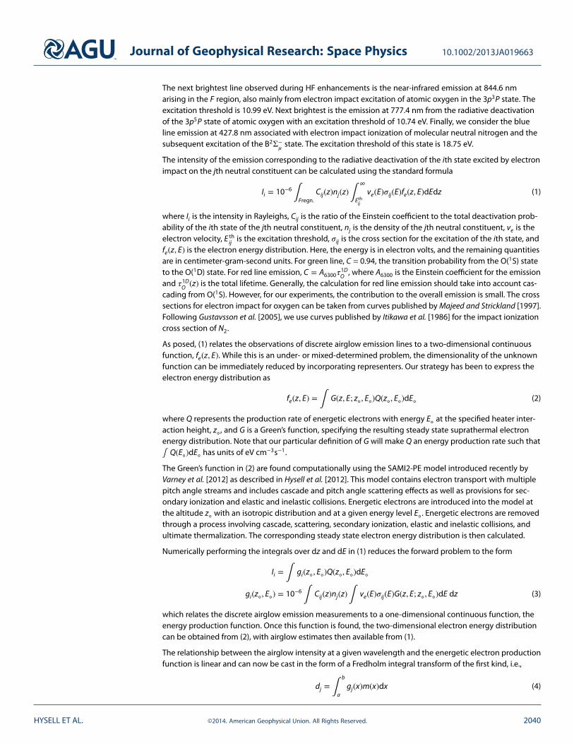
The intensity of the emission corresponding to the radiative deactivation of the ith state excited by electronimpact on the jth neutral constituent can be calculated using the standard formula

Ii = 10−6 ∫Fregn.Cij(z)nj(z)∫

∞

Ethij

ve(E)𝜎ij(E)fe(z, E)dEdz (1)

where Ii is the intensity in Rayleighs, Cij is the ratio of the Einstein coefficient to the total deactivation prob-ability of the ith state of the jth neutral constituent, nj is the density of the jth neutral constituent, ve is theelectron velocity, E th

ij is the excitation threshold, 𝜎ij is the cross section for the excitation of the ith state, andfe(z, E) is the electron energy distribution. Here, the energy is in electron volts, and the remaining quantitiesare in centimeter-gram-second units. For green line, C = 0.94, the transition probability from the O(1S) stateto the O(1D) state. For red line emission, C = A6300𝜏

1DO , where A6300 is the Einstein coefficient for the emission

and 𝜏1DO (z) is the total lifetime. Generally, the calculation for red line emission should take into account cas-

cading from O(1S). However, for our experiments, the contribution to the overall emission is small. The crosssections for electron impact for oxygen can be taken from curves published by Majeed and Strickland [1997].Following Gustavsson et al. [2005], we use curves published by Itikawa et al. [1986] for the impact ionizationcross section of N2.

As posed, (1) relates the observations of discrete airglow emission lines to a two-dimensional continuousfunction, fe(z, E). While this is an under- or mixed-determined problem, the dimensionality of the unknownfunction can be immediately reduced by incorporating representers. Our strategy has been to express theelectron energy distribution as

fe(z, E) = ∫ G(z, E; z◦, E◦)Q(z◦, E◦)dE◦ (2)

where Q represents the production rate of energetic electrons with energy E◦ at the specified heater inter-action height, z◦, and G is a Green’s function, specifying the resulting steady state suprathermal electronenergy distribution. Note that our particular definition of G will make Q an energy production rate such that∫ Q(E◦)dE◦ has units of eV cm−3s−1.

The Green’s function in (2) are found computationally using the SAMI2-PE model introduced recently byVarney et al. [2012] as described in Hysell et al. [2012]. This model contains electron transport with multiplepitch angle streams and includes cascade and pitch angle scattering effects as well as provisions for sec-ondary ionization and elastic and inelastic collisions. Energetic electrons are introduced into the model atthe altitude z◦ with an isotropic distribution and at a given energy level E◦. Energetic electrons are removedthrough a process involving cascade, scattering, secondary ionization, elastic and inelastic collisions, andultimate thermalization. The corresponding steady state electron energy distribution is then calculated.

Numerically performing the integrals over dz and dE in (1) reduces the forward problem to the form

Ii = ∫ gi(z◦, E◦)Q(z◦, E◦)dE◦

gi(z◦, E◦) = 10−6 ∫ Cij(z)nj(z)∫ ve(E)𝜎ij(E)G(z, E; z◦, E◦)dE dz (3)

which relates the discrete airglow emission measurements to a one-dimensional continuous function, theenergy production function. Once this function is found, the two-dimensional electron energy distributioncan be obtained from (2), with airglow estimates then available from (1).

The relationship between the airglow intensity at a given wavelength and the energetic electron productionfunction is linear and can now be cast in the form of a Fredholm integral transform of the first kind, i.e.,

dj = ∫b

agj(x)m(x)dx (4)

HYSELL ET AL. ©2014. American Geophysical Union. All Rights Reserved. 2040

Journal of Geophysical Research: Space Physics 10.1002/2013JA019663

Figure 1. Ion line power versus range and time obtained with the UHF diagnostic radar at HAARP looking parallel to B(15◦ zenith angle). The radar has a peak pulse power of about 125 kW. The pulse length was 996 μs with a 249-bit phasecode, providing 600 m range resolution. The pulse repetition rate was 100 Hz, and the data were processed with 20-pulsemoving averages.

where dj represents airglow observations at different wavelengths j (the data), m(x) represents theproduction function at some energy level (the model), and gj(x) defined above plays the role of atransfer function.

The integral transform is from a continuous model to a discrete set of data. A least squares method mini-mizes the discrepancy between measured data and the data predicted by the model. This method fails inunderdetermined or mixed-determined problems for which such a model is not unique. In contrast, themethod of Backus and Gilbert minimizes the discrepancy between the model implied by measured dataand the model implied by the data that the model itself predicts. The solution is unique even for underde-termined problems. However, the Backus and Gilbert model is not guaranteed to reproduce closely the datafrom which they are derived. Nor they are guaranteed to be stable. Hysell et al. [2012] addressed both short-comings by augmenting the standard Backus and Gilbert solution. For the present analysis, a small amountof damping was incorporated in the algorithm to minimize the discrepancy between the predicted andactual data and to improve overall stability. For details regarding augmentation and implementation of theBackus and Gilbert method to the airglow inversion problem, see Hysell et al. [2012].

Figure 2. Spectrometer data for March 12, 2013.Bottom panel: airglow intensity versus wavelength and UT. Top panel:airglow intensity versus wavelength for the indicated time. Right panel: airglow intensity for 427.8 nm (blue), 557.7 nm(green), 630.0 nm (red) 777.4 nm (brown), and 844.6 nm (black). Units are Rayleighs.

HYSELL ET AL. ©2014. American Geophysical Union. All Rights Reserved. 2041

Journal of Geophysical Research: Space Physics 10.1002/2013JA019663

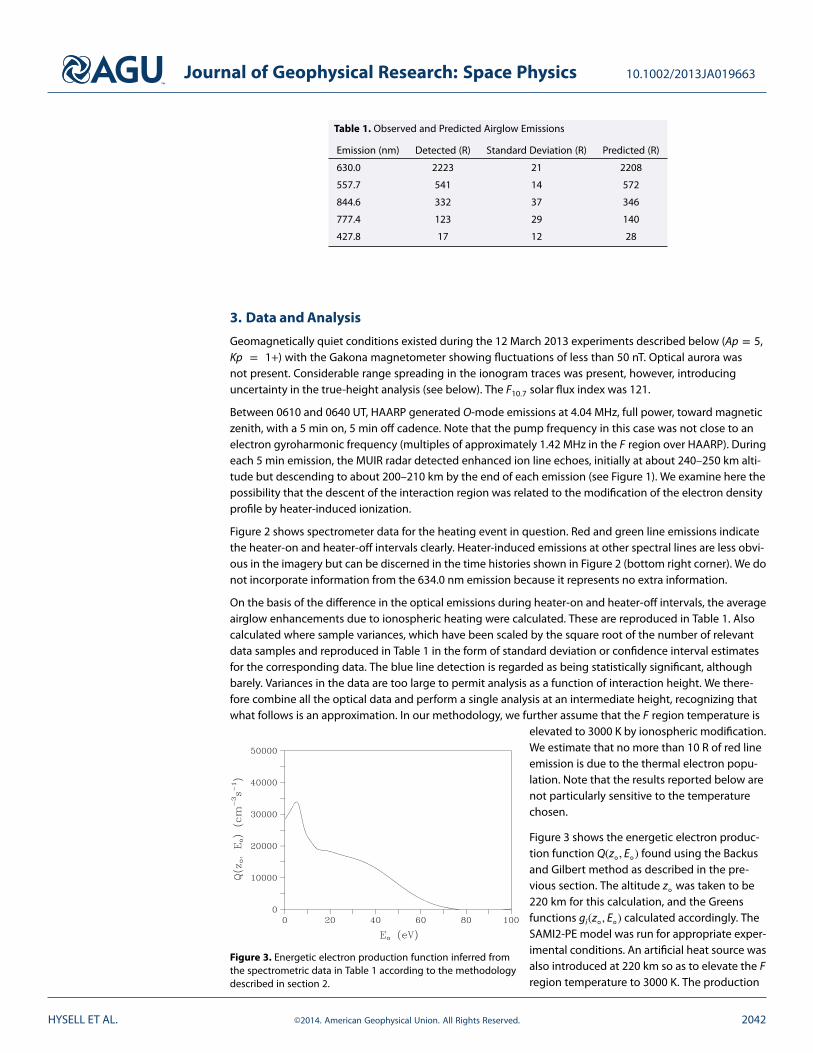
Table 1. Observed and Predicted Airglow Emissions

Emission (nm) Detected (R) Standard Deviation (R) Predicted (R)

630.0 2223 21 2208

557.7 541 14 572

844.6 332 37 346

777.4 123 29 140

427.8 17 12 28

3. Data and Analysis

Geomagnetically quiet conditions existed during the 12 March 2013 experiments described below (Ap = 5,Kp = 1+) with the Gakona magnetometer showing fluctuations of less than 50 nT. Optical aurora wasnot present. Considerable range spreading in the ionogram traces was present, however, introducinguncertainty in the true-height analysis (see below). The F10.7 solar flux index was 121.

Between 0610 and 0640 UT, HAARP generated O-mode emissions at 4.04 MHz, full power, toward magneticzenith, with a 5 min on, 5 min off cadence. Note that the pump frequency in this case was not close to anelectron gyroharmonic frequency (multiples of approximately 1.42 MHz in the F region over HAARP). Duringeach 5 min emission, the MUIR radar detected enhanced ion line echoes, initially at about 240–250 km alti-tude but descending to about 200–210 km by the end of each emission (see Figure 1). We examine here thepossibility that the descent of the interaction region was related to the modification of the electron densityprofile by heater-induced ionization.

Figure 2 shows spectrometer data for the heating event in question. Red and green line emissions indicatethe heater-on and heater-off intervals clearly. Heater-induced emissions at other spectral lines are less obvi-ous in the imagery but can be discerned in the time histories shown in Figure 2 (bottom right corner). We donot incorporate information from the 634.0 nm emission because it represents no extra information.

On the basis of the difference in the optical emissions during heater-on and heater-off intervals, the averageairglow enhancements due to ionospheric heating were calculated. These are reproduced in Table 1. Alsocalculated where sample variances, which have been scaled by the square root of the number of relevantdata samples and reproduced in Table 1 in the form of standard deviation or confidence interval estimatesfor the corresponding data. The blue line detection is regarded as being statistically significant, althoughbarely. Variances in the data are too large to permit analysis as a function of interaction height. We there-fore combine all the optical data and perform a single analysis at an intermediate height, recognizing thatwhat follows is an approximation. In our methodology, we further assume that the F region temperature is

Figure 3. Energetic electron production function inferred fromthe spectrometric data in Table 1 according to the methodologydescribed in section 2.

elevated to 3000 K by ionospheric modification.We estimate that no more than 10 R of red lineemission is due to the thermal electron popu-lation. Note that the results reported below arenot particularly sensitive to the temperaturechosen.

Figure 3 shows the energetic electron produc-tion function Q(z◦, E◦) found using the Backusand Gilbert method as described in the pre-vious section. The altitude z◦ was taken to be220 km for this calculation, and the Greensfunctions gi(z◦, E◦) calculated accordingly. TheSAMI2-PE model was run for appropriate exper-imental conditions. An artificial heat source wasalso introduced at 220 km so as to elevate the Fregion temperature to 3000 K. The production

HYSELL ET AL. ©2014. American Geophysical Union. All Rights Reserved. 2042

Journal of Geophysical Research: Space Physics 10.1002/2013JA019663

Figure 4. Energetic electron spectrum associated with the production function in Figure 2.

function seems to be characterized by two populations or sources. Combining the production function withthe Green’s functions then leads to the energetic electron distribution estimate, which is shown in Figure 4.

Finally, Figure 5 shows the consequences of all the modeled ionospheric modification effects on the electronnumber density and temperature profiles computed using SAMI2-PE. Curves are shown for (1) backgroundconditions, absent ionospheric modification, (2) the case where a heat source alone is introduced at 220km altitude, and (3) the case where an energetic electron population governed by the estimated fluxes inFigure 4, only scaled upward by a multiplicative factor of 5 (see below), is also present. Estimates of the back-ground electron density profile at 0625 UT derived from manually scaled ionosonde data are also shownfor reference. We note first that ohmic heating is much more significant than heating due to suprathermalelectrons, although the latter effect is not negligible. Ohmic heating alone does not significantly alter thenumber density at the 220 km interaction altitude, however, although it does raise it somewhat at lower alti-tudes. This is due to temperature dependence in the recombination rate. (See also Blagoveshchenskaya et al.[2009] who treated temperature-dependent recombination in some detail.)

Figure 5. Equilibrium temperature (red curves) and density profiles (black curves) simulated for (1) background condi-tions (solid line), (2) including a heat source at 220 km altitude (short dashed line), and (3) including also an energeticelectron population governed by the results in Figure 3, only scaled upward by a factor of 5 (long dashed line). Opencircles show the results of true-height analysis of ionosonde data from 0625 UT during a heater-off interval.

HYSELL ET AL. ©2014. American Geophysical Union. All Rights Reserved. 2043

Journal of Geophysical Research: Space Physics 10.1002/2013JA019663

Figure 6. Statistical data from the HAARP TelescopicImager at 0603 UT, green line, background subtracted. Aportion of the image with a field of view comparable tothe spectrometer was examined in constructing this plot.The solid line shows the number of pixels with intensitiesfalling in the given bin in Rayleighs (log scale), and thedashed line shows the fraction of pixels with intensity lessthan the given value.

The augmented energetic electron population,meanwhile, increases the plasma number densityby more than a factor of 2 in some places. Withoutthe aforementioned factor of 5 scaling, meanwhile,the effect of the energetic electrons would beproportionally smaller and difficult to discern.

The amplitude scaling factor is not arbitrary butreflects the filamentary, spatially intermittent natureof the airglow observed during heating experi-ments. The airglow is not beam filling, and electronimpact excitation and ionization is occurring manytimes more rapidly in the affected filaments thanthe average rate. The factor of 5 is based on greenline imagery from the HAARP Telescopic imager. Thespatiotemporal variability of heater-induced airglowdetected with this imager has been documentedextensively by Kendall et al. [2010]. (Temporal vari-ability is masked in our spectrometer data by thelong integration times involved.) Histograms rank-ing pixel count versus intensity constructed fromindividual images have been found to have long,high-intensity tails. An example of such a histogram

is shown in Figure 6 for an image acquired during one of the heater-on periods. For this case, the aver-age intensity is approximately 740 R, but the distribution intensity has a long tail with an appreciablebump around 3.7 kR, 5 times the average. Approximately 1% of the pixels in the image have intensitiesabove 3.7 kR.

4. Summary and Conclusions

In this paper, we estimated the suprathermal electron population versus altitude and energy during anF region ionospheric modification experiment characterized by unusually bright airglow on the basis ofobserved emissions at five optical wavelengths. Our inverse method was based on a variation of the clas-sic Backus and Gilbert approach and utilized Green’s functions to reduce the dimensionality of the problem.The method is nonparametric, in contrast to the method of Gustavsson and Eliasson [2008] who used air-glow emissions to set the parameters of a physics-based electron acceleration model. Whereas the lattermethod naturally gives more physical insight into ionospheric modification experiments, the prior proba-bility implied could be regarded as being overly restricted to the degree that the acceleration mechanism isnot fully understood.

Our results indicate that the suprathermal electron population is sufficient for producing significant artificialionization but with qualifications. If the electron acceleration were distributed homogeneously throughoutthe modified volume, its effect on the electron density profile would be small compared to the effect ofdirect heating. However, imaging has shown that the airglow productions is inhomogeneous and spatiallyintermittent. If the electron acceleration is also spatially inhomogeneous, its effect could be significant insmall regions where it is most highly concentrated, dominating variations in the electron density profile.In this scenario, which is supported by airglow imagery, the induced ionization should more accurately beconsidered filamentary rather than layer like. The extra ionization provides feedback that further amplifiesthe degree of inhomogeneity initially present in the plasma.

ReferencesAdeishvili, T. S., A. V. Gurevich, S. B. Liakhov, G. G. Managadze, G. M. Milikh, and I. S. Shliuger (1978), Ionospheric emission caused by an

intense radio wave, Sov. J. Plasma Phys., 4, 1293–1301.Aster, R. C., B. Borchers, and C. H. Thurber (2005), Parameter Estimation and Inverse Problems, Elsevier, New York.Backus, G., and F. Gilbert (1968), The resolving power of gross Earth data, Geophys. J. R. Astron. Soc., 16, 169–205.Backus, G., and F. Gilbert (1970), Uniqueness in the inversion of inaccurate gross Earth data, Philos. Trans. R. Soc. London, Ser. A, 266,

123–192.

AcknowledgmentsThis project was supported by DARPAthrough contract HR0011-09-C-0099.Additional support came from theHigh Frequency Active AuroralResearch Program (HAARP) and fromthe Office of Naval Research and theAir Force Research Laboratory undergrant N00014-07-1-1079 to Cornell.Work at AFRL was supported by theAir Force Office of Scientific Research.The research of J.D.H. was supportedby NRL Base Funds. R.H.V. is supportedby the NASA Living With a Star JackEddy Postdoctoral Fellowship program,administered by the University Cor-poration for Atmospheric Research.The National Center for AtmosphericResearch is sponsored by the NationalScience Foundation. The GakonaDigisonde is operated by AFRL, andthe data are available at the Low-ell GIRO Data Center. Ivan Galkin atthe University of Massachusetts Low-ell assisted with the Digisonde datainterpretation.

Robert Lysak thanks Herbert Carlsonand an anonymous reviewer for theirassistance in evaluating this paper.

HYSELL ET AL. ©2014. American Geophysical Union. All Rights Reserved. 2044

Journal of Geophysical Research: Space Physics 10.1002/2013JA019663

Bernhardt, P. A., C. A. Tepley, and L. M. Duncan (1989), Airglow enhancements associated with plasma cavities formed during ionosphericheating experiments, J. Geophys. Res., 94, 9071–9092.

Biondi, A. A., D. P. Sipler, and R. D. Hake (1970), Optical 𝜆-6300 detection of radio frequency heating of electrons in the F region, J.Geophys. Res., 75, 6421–6424.

Blagoveshchenskaya, N. F., H. C. Carlson, V. A. Kornienko, T. D. Borisova, M. T. Rietveld, T. K. Yeoman, and A. Brekke (2009), Phenom-ena induced by powerful HF pumping towards magnetic zenith with a frequency near the F-region critical frequency and the thirdelectron gyro harmonic frequency, Ann. Geophys., 27, 131–145.

Carlson, H., V. Wickwar, and G. Mantas (1982), Observations of fluxes of suprathermal electrons accelerated by HF excited instabilities, J.Atmos. Terr. Phys., 44(12), 1089–1100.

Carlson, H. C. (1993), High-power HF modification: Geophysics, span of EM effects, and energy budget, Adv. Space Res., 13, 15–24,doi:10.1016/0273–1177(93)90046–E.

Djuth, F. T., T. R. Pedersen, E. A. Gerken, P. A. Bernhardt, C. A. Selcher, W. A. Bristow, and M. J. Kosch (2005), Ionospheric modification attwice the electron cyclotron frequency, Phys. Rev. Lett., 94, 125001.

Eliasson, B., X. Shao, G. M. Milikh, E. V. Mishin, and K. D. Papadopoulos (2012), Numerical modeling of artificial ionospheric layers drivenby high-power HF-heating, J. Geophys. Res., 117, A10321, doi:10.1029/2012JA018105.

Gurevich, A. V. (2007), Nonlinear effects in the ionosphere, Usp. Fizicheskikh Nauk., 177(11), 1145–1177.Gurevich, A. V., H. C. Calson, Y. V. Medvedev, and K. P. Zybin (2004), Langmuir turbulence in ionospheric plasma, Plasma Phys. Rep., 30(12),

995–1005.Gustavsson, B., and B. Eliasson (2008), HF radio wave acceleration of ionospheric electrons: Analysis of HF-induced optical enhancements,

J. Geophys. Res., 113, A08319, doi:10.1029/2007JA012913.Gustavsson, B., B. U. E. Brändström, Å. Steen, T. Sergeinko, T. B. Leyser, M. T. Rietveld, T. Aso, and M. Ejiri (2003), Nearly simultaneous

images of HF-pump enhanced airglow at 6300 Å and 5577 Å, Geophys. Res. Lett., 29(24), 2220, doi:10.1029/2002GL015350.Gustavsson, B., et al. (2001), First tomographic estimate of volume distribution of enhanced airglow emission caused by HF pumping, J.

Geophys. Res., 106, 29,105–29,123.Gustavsson, B., et al. (2005), The electron distribution during HF pumping, a picture painted with all colours, Ann. Geophys., 23,

1747–1754.Haslett, J. C., and L. R. Megill (1974), A model of the enhanced airglow excited by RF radiation, Radio Sci., 9, 1005–1019.Huba, J. D., G. Joyce, and J. A. Fedder (2000), Sami2 is another model of the ionosphere (SAMI2): A new low-latitude ionospheric model,

J. Geophys. Res., 105, 23,035–23,054.Hysell, D. L., R. H. Varney, M. N. Vlasov, E. Nossa, B. Watkins, T. Pedersen, and J. D. Huba (2012), Estimating the electron energy

distribution during ionospheric modification from spectrographic airglow measurements, J. Geophys. Res., 117, A02317,doi:10.1029/2011JA017187.

Itikawa, Y., M. Hayashi, A. Ichimaru, K. Onda, K. Sakimoto, K. Takayanagi, M. Nakamura, H. Nishimura, and T. Takayamagi (1986),Cross-sections for collisions of electrons and photons with nitrogen molecules, J. Phys. Chem. Ref. Data, 15, 985–1010.

Kendall, E., R. Marshall, R. T. Parris, A. Bhatt, A. Coster, T. Pedersen, P. Bernhardt, and C. Selcher (2010), Decameter structurein heater-induced airglow at the High frequency Active Auroral Research Program facility, J. Geophys. Res., 115, A08306,doi:10.1029/2009JA015043.

Majeed, T., and D. J. Strickland (1997), New survey of electron impact cross-sections for photoelectron and auroral electron energy losscalculations, J. Phys. Chem. Ref. Data, 26, 335–349.

Mantas, G. P. (1994), Large 6300-Å airglow intensity enhancements observed in ionosphere heating experiments are excited by thermalelectrons, J. Geophys. Res., 99, 8993–9002.

Mantas, G. P., and H. C. Carlson (1996), Reinterpretation of the 6300-Å airglow enhancements observed in ionosphere heatingexperiments based on analysis of Platville, Colorado, data, J. Geophys. Res., 101, 195–209.

Menke, W. (1984), Geophysical Data Analysis: Discrete Inverse Theory, Academic, New York.Mutiso, C. K., J. M. Hughes, G. G. Sivjee, T. Pedersen, B. Gustavsson, and M. J. Kosch (2008), Previously unreported optical emissions

generated during ionospheric heating, Geophys. Res. Lett., 35, L14103, doi:10.1029/2008GL034563.Pedersen, T., B. Gustavsson, E. Mishin, E. MacKenzie, H. C. Carlson, M. Starks, and T. Mills (2009), Optical ring formation and ionization

production in high power HF heating experiments at HAARP, Geophys. Res. Lett., 36, L18107, doi:10.1029/2009GL040047.Pedersen, T., B. Gustavsson, E. Mishin, E. Kendall, T. Mills, H. C. Carlson, and A. L. Snyder (2010), Creation of artificial ionospheric layers

using high-power HF waves, Geophys. Res. Lett., 37, L02106, doi:10.1029/2009GL041895.Rose, G., B. Grandal, E. Neske, W. Ott, K. Spenner, J. Holtet, K. Måseide, and J. Trøim (1985), Experimental results from the HERO project:

In situ measurements of ionospheric modifications using sounding rockets, J. Geophys. Res., 90, 2851–2860.Tarantola, A. (1987), Inverse Theory, Elsevier, New York.Varney, R. H., W. Swartz, D. Hysell, and J. Huba (2012), SAMI2-PE: A model of the ionosphere including multi-stream interhemispheric

photoelectron transport, J. Geophys. Res., 117, A06322, doi:10.1029/2011JA017280.

HYSELL ET AL. ©2014. American Geophysical Union. All Rights Reserved. 2045