Noname manuscript No.

(will be inserted by the editor)

Heat Transfer Coefficients during Quenching of Steels

H. S. Hasan · M. J. Peet · J. M. Jalil · H.

K. D. H. Bhadeshia

Received: date / Accepted: date

Abstract Heat transfer coefficients for quenching in water have been measured as a

function of temperature using steel probes for a variety of iron alloys. The coefficients

were derived from measured cooling curves combined with calculated heat–capacities.

The resulting data were then used to calculate cooling curves using the finite vol-

ume method for a large steel sample and these curves have been demonstrated to be

consistent with measured values for the large sample. Furthermore, by combining the

estimated cooling curves with time–temperature–transformation diagrams it has been

possible to predict the variation of hardness as a function of distance via the quench

factor analysis. The work should prove useful in the heat treatment of the steels studied,

some of which are in the development stage.

Keywords heat transfer coefficient · steel · hardness prediction · phase transfor-

mation

H. S. HasanThe University of Technology, BaghdadDepartment of Electromechanical EngineeringBaghdad, Iraq

M. J. PeetUniversity of CambridgeDepartment of Materials Science and MetallurgyPembroke Street, Cambridge CB2 3QZ, U. K.

J. M. JalilThe University of Technology, BaghdadDepartment of Electromechanical EngineeringBaghdad, Iraq

H. K. D. H. Bhadeshia (corresponding author)University of CambridgeDepartment of Materials Science and MetallurgyPembroke Street, Cambridge CB2 3QZ, U. K.E-mail: hkdb@cam.ac.uk

2

1 Introduction

Quenching is a widely used commercial process in which steel components in their

austenitic state are immersed in a liquid at a much lower temperature, resulting in

rapid cooling, and under appropriate circumstances, the hardening of the steel. This

simple description hides the complexity of the process, in which the transfer of heat to

the quenching medium involves many phenomena at the steel/liquid interface (which

may enclose a vapour gap), some of which are expressed in terms of a heat–transfer

coefficient (h) which is a function of the steel and quenchant. The heat flux across

the interface is given by q = h∆T where ∆T is the temperature difference between

the source and the sink. The heat transfer coefficient is often approximated to be

constant, and this may be valid over specified temperature ranges. However, it can vary

significantly with temperature [22], in which case a reliable estimation of the cooling

behaviour of a quenched component, and any subsequent calculations of structure

and properties, requires accurate and temperature–dependent heat transfer coefficients

[8, 25, 27].

The heat transfer coefficient can be measured experimentally using a cylindrical

probe with one or more thermocouples attached. The probe is quenched and the varia-

tion in temperature as a function of time is measured [2, 16, 21] and the resulting data

interpreted in order to determine h. The probe diameter is usually in excess of 12.5 mm,

with a length at least four times the diameter in order to minimise end–cooling effects.

The probes are usually made from metals which do not undergo phase transformations,

such as Inconel 600 [7, 9, 12, 19], silver [12] or austenitic steel [10, 30]. This avoids the

influence of enthalpy changes due to phase transformations; by the same logic, it does

not reveal the effect of such changes on the heat–transfer coefficient, which may be

important since the majority of heat–treatments are conducted on transforming steels.

The purpose of the present work was to undertake detailed measurements of the

heat–transfer coefficients of a number of transforming steels, and to combine the data

thus collected with a variety of mathematical models to enable the prediction of the

hardness following the quenching heat–treatments.

2 Method

Equipment was designed consisting of a data–acquisition system, a small tube furnace,

a 1

4l beaker containing the quenchant and K–type thermocouple, Fig. 1. The probe

material was, after machining, cleaned in an ultrasonic bath containing methanol. The

1 mm diameter thermocouple was inserted into the cylindrical probe together with

some fine graphite powder for better thermal contact. It was held in position using

a screw from the side and any gap between the probe and thermocouple sealed using

alumina paste which was furnace–hardened for 8 h at 200◦C in order to avoid erroneous

readings from the leakage of quenchant into the thermocouple. The probe assembly was

placed vertically into a tube furnace with a hot–zone of 13 cm, through a guide–hole

and held at 850◦C for 5 min before allowing the probe to fall and be brought to a

standstill by the flange when it enters the quenchant in the beaker. The quenchant

volume is sufficiently large to ensure no significant change in its temperature due to

the quench. Throughout this process, data were collected on a computer at a rate of

1000 temperature readings per second.

3

The probe dimensions were determined by calculating the Biot number, Bi =

hL/k ≤ 0.1, where L is the characteristic length and k the thermal conductivity. The

latter is typically 50Wm−1 K−1 and assuming a heat transfer coefficient of 104 Wm−2K−1

permits the estimation of the required length of the probe. The condition that Bi ≤ 0.1

is equivalent to assuming that the controlling heat–transfer resistance is confined to

the external coolant, and the establishment of quasi–flat temperature profiles inside

the sample [1]. The probe length is five times its diameter in so that end–effects can

be neglected and to justify the assumption that only radial heat–flow occurs at its

half–length. The surface finish of the probe was fixed by machining and grinding.

The probe materials investigated are listed in Table 1; they were selected from

available alloys to cover a range of carbon concentrations and hardenabilities; alloy C is

from a new class of bulk nanostructured–steels which transform at very low homologous

temperatures [6].

All reported hardness determinations used a 30 kg load and the values quoted are

averages from a minimum of 3 indents.

Table 1 Chemical compositions of the probe materials in wt%.

Steel C Si Mn Ni Mo Cr Al Co Cu

A 0.16 0.16 0.67 0.08 0.02 0.06 - - -

B 0.15 1.19 1.50 0.08 0.31 1.19 0.02 - 0.136

C 0.78 1.60 2.02 - 0.25 1.01 1.37 3.87 -

D 0.55 0.22 0.77 0.15 0.05 0.20 - - -

E 0.54 0.20 0.74 0.17 0.05 0.20 - - -

F 0.16 0.22 0.30 2.93 0.39 1.47 0.28 - 0.01

3 Data Analysis and Results

A minimum of three quenching experiments were performed in each case to assess re-

peatability. To reduce the influence of noise, the time–temperature data were smoothed

using a rolling average of 11 points in order to calculate the cooling rate by differentia-

tion. The temperature–dependent heat–transfer coefficient is then given by [17, 18, 23]:

h =ρV CP T

A(TS − T∞)(1)

where CP is the specific heat capacity at constant pressure, V and A the sample

volume and surface area respectively, ρ = 7858 kgm−3 the density which is assumed to

be constant, and T the instantaneous cooling rate. The heat capacity was calculated as

a function of temperature using the thermodynamic software MTDATA [24] with the

SGTE database, for the steel in the austenitic state since the alloys were expected to

remain untransformed until the martensite–start (MS) temperature is reached. Typical

results for alloy D are illustrated in Fig. 2. The data for equilibrium mixtures of ferrite

and cementite are also plotted because as will be seen later, the largest of samples do

4

not completely transform into martensite; in such cases, the equilibrium calculation

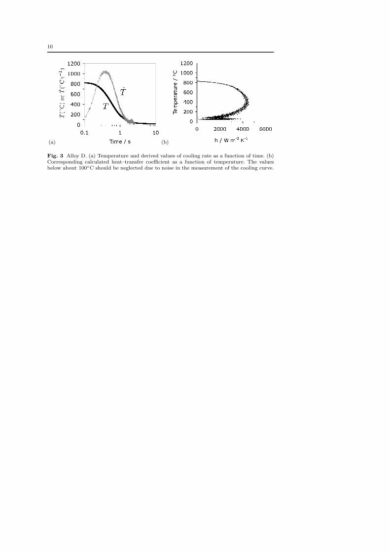
represents an upper limit for the heat capacity. Fig. 3 shows the measured cooling

and cooling–rate curves for alloy D, together with the derived heat transfer coefficient

as a function of surface temperature. The readings below about 100◦C become noisy

because the difference in temperature between adjacent recordings becomes comparable

to the accuracy of the thermocouple. These curves are, over the temperature range

600–850◦C, typical of all the experiments and the complete set is illustrated in Fig. 4.

However, there are important differences with respect to alloys A and C, both of

which have exhibited a high cooling rate during the quench at temperatures below

about 400◦C, Fig. 4a. Alloy A does not have sufficient hardenability in order to ensure

a fully martensitic microstructure on quenching (Fig. 5a); the sample has a hardness of

only 260HV in its final state (Table 2). Allotriomorphic ferrite forms at high tempera-

tures, so that the amount of austenite which undergoes martensitic transformation is

reduced, resulting in a smaller enthalpy change and hence a faster cooling rate (relative

to those alloys which become fully martensitic) at low temperatures during the quench.

In the case of alloy C, the hardenability is sufficient to yield a martensitic microstruc-

ture (Fig. 5b)with a hardness of 730 HV, but calculations using MTDATA revealed

that the enthalpy change at the MS = 202◦C for alloy C is ∆H = 4600 Jmol−1, which

compares with ∆H = 6000–7000 Jmol−1 for the other steels, Fig. 6. The smaller re-

lease in heat on transformation is consistent with the more rapid cooling rate at low

temperatures for alloy C.

Table 2 Vickers hardness data measured using a 30 kg load following quenching. The maxi-mum hardness refers to samples that were quenched into agitated water at 20◦C, after austeni-tisation at 950◦C for 30min; these values are necessary in the quench factor analysis. Themartensite–start temperatures are calculated using a neural network based on the data from[29].

Steel MS/◦C Probe hardness Maximum Hardness

A 455 260±9 351±8

B 435 456±34 471±6

C 202 753±2 748±7

D 269 728±13 731±1

E 276 735±15 720±6

F 405 458±7 473±13

4 Application of Heat Transfer Coefficients

The work presented below was done to demonstrate the utility of the measured heat–

transfer coefficients for samples bigger than the probes described earlier and for the

Fe–0.55 wt%, steel D, Table 1). A large cylinder, 52mm diameter, 20mm long was in-

strumented with three thermocouples place in 1mm diameter axial holes drilled 10mm

into the sample. The holes were located at the centre of the cylinder, about 0.5mm

from the surface, and half way along its radius. The sample was then austenitised and

quenched into water while recording the cooling curves.

5

The measured cooling curves were compared against those calculated using dis-

cretised heat flow equations based on a finite volume method described elsewhere in

detail [14, 28]. The calculations require a knowledge of the density, thermal conduc-

tivity (obtained from a neural network model [15]), and the relevant measured heat

transfer coefficients (Fig. 4). The heat capacity was once again calculated as a func-

tion of temperature using MTDATA, allowing ferrite, cementite and austenite to exist

(Fig. 2); the peak in capacity that occurs at the Curie temperature was truncated by

describing the variation using a polynomial equation in order to avoid computational

difficulties [13].

The calculated and measured curves are presented in Fig. 7. There is reasonable

agreement except at the very surface, and there seems to be some influence of the

latent heat of transformation on the measured curves, which has not been taken into

account in the calculations. The microstructure of the sample was characterised met-

allographically and ranged from martensite near the surface to a mixture of ferrite and

pearlite at the centre (the micrographs are omitted for brevity).

It is possible to use the cooling information to calculate the variation in hardness

because in quench factor analysis there is a correlation between the cooling curve and

a property of interest (in this case hardness). Quench factor analysis was originally

proposed by Evancho and Staley [11] and has since then been justified and developed

further; a recent paper [26] is a good summary of its modern interpretation. In essence,

the variation of the normalised value of hardness is expressed in terms of the quench

factor Q as:

H −Hmin

Hmax −Hmin

= exp{k1Q} with Q =

∫ tf

to

dt

tC(2)

where H is the hardness and the subscripts represent minimum and maximum values

of the hardness, and k1 represents the logarithm of the fraction of transformation.

tC represents the critical time required to achieve a given fraction of phase trans-

formation. The maximum hardness is taken to be that of martensite, measured by

quenching a 4mm sample of the steel into water following austenitisation at 950◦C for

30min. This was confirmed to give a fully martensitic microstructure with a hardness

Hmax = 731HV. The value of Hmin was obtained by similarly austenisiting but then

transforming isothermally at 650◦C for 2 h in order to obtain pearlite with a hard-

ness of 185HV. There was no significant scatter observed in these values, which were

constant within ±1HV.

Time–temperature transformation (TTT) diagrams were calculated for steel D us-

ing the thermodynamic and kinetic methods described in [3–5]1. The calculation is

illustrated in Fig. 8a with the imposed calculated cooling curves. The TTT curves

represent the onset of transformation, the first detectable quantity, taken to represent

0.05 fraction of reaction, the logarithm of which gives k1. Fig. 8b shows the comparison

between the calculated and measured hardness values, with good agreement given the

lack of assumptions in the analysis. Further improvements may be possible by better

accounting for the the latent heat of transformation and specific heat capacity. How-

1 The software for doing these calculations is available freely on

http://www.msm.cam.ac.uk/map/steel/programs/mucg46-b.html

6

ever, this is not trivial because it would be necessary to have a coupling with detailed

phase transformation models to represent the evolution of microstructure.

In the present work we have used steel probes to determine the heat–transfer co-

efficients given that the interest is in the heat–treatment of iron alloys. Fig. 9a shows

h measured in the present work using the steel probe for steel D, and data from the

literature on the JIS and Inconel 600 probes [20]. Fig. 9 shows that better agreement

is obtained using the heat transfer coefficients determined using the steel probe.

5 Conclusions

1. A probe has been developed to determine the heat transfer coefficient of steel.

The probe dimensions were fixed by ensuring an appropriate Biot number so that

the probe temperature can be as uniform as possible during the course of the

experiments.

2. The confidence in the measured heat transfer coefficients is supported by the fact

that reasonable predictions could be made of the cooling curves when applied to a

steel sample much larger than the probes.

3. The heat–transfer coefficients when combined with calculated cooling and time–

temperature–transformation curves, can with the help of the quench factor method

enable the estimation of hardness variation as a function of distance.

4. It has been demonstrated that the steel probe, which replicates phase transforma-

tions during the course of cooling, is the best for determining the heat–transfer

coefficients.

Acknowledgements The authors are grateful to British Universities Iraq Consortium forfunding this work, to the Ministry of Education in Iraq and to the University of Cambridgefor the provision of laboratory facilities.

References

1. Arpaci VS (1966) Conduction heat transfer. Addison–Wesley Publication Com-

pany, Reading, Massachusetts, USA

2. Bates CE, Totten GE, Clinton NA (1993) Handbook of Quenchants and Quenching

Technology. ASM International, Materials Park, Ohio, USA

3. Bhadeshia HKDH (1981) The driving force for martensitic transformation in steels.

Metal Science 15:175–177

4. Bhadeshia HKDH (1981) Thermodynamic extrapolation and the martensite-start

temperature of substitutionally alloyed steels. Metal Science 15:178–150

5. Bhadeshia HKDH (1982) A thermodynamic analysis of isothermal transformation

diagrams. Metal Science 16:159–165

6. Caballero FG, Bhadeshia HKDH, Mawella KJA, Jones DG, Brown P (2002) Very

strong, low–temperature bainite. Materials Science and Technology 18:279–284

7. Chen N, Zhang W, Gao C, Liao B, Pan J (2006) The effects of probe geometric

shape on the cooling rate curves obtained from different quenchants. Diffusion and

defect data Solid state data Part B, Solid state phenomena 118:227–231

8. Chen N, Han L, Zhang W, Hao X (2007) Enhancing mechanical properties and

avoiding cracks by simulation of quenching connecting rods. Materials Letters

61:3021–3024

7

9. Chen N, Han L, Zhang W, Hao X (2007) Enhancing mechanical properties and

avoiding cracks by simulation of quenching connecting rods. Materials Letters

61:3021–3024

10. Chen X, Meekisho L, Totten GE (1999) Computer–aided analysis of the quenching

probe test. In: Wallis RA, Walton HW (eds) Heat Treating: Proceedings of the

18th Conference, ASM International, Materials Park, Ohio, USA

11. Evancho JW, Stanley JT (1974) Kinetics of precipitation in aluminium alloys dur-

ing continuous cooling. Metallurgical Transactions 5:43–47

12. Funatani K, Narazaki M, Tanaka M (1999) Comparisons of probe design and cool-

ing curve analysis methods. In: Midea SJ, Pfaffmann GD (eds) 19th ASM Heat

Treating Society Conference, ASM International, Materials Park, Ohio, USA, pp

255–263

13. Goldak J, Bibby M, Moore J, House R, Patel B (1986) Computer modeling of heat

flow in welds. Metallurgical Transactions B 17:587–600

14. Hasan HS (2009) Heat transfer and phase transformations in steels. PhD thesis,

University of Technology, Bhagdad, Bhagdad, Iraq

15. Hasan HS, Peet M (2009) Map steel thermal. Computer program

http://www.msm.cam.ac.uk/map/steel/programs/thermalmodel.html, University

of Cambridge

16. Hernandez-Morales B, Tellez-Martinez JS, Ingalls-Cruz A, Godlınez JB (1999)

Cooling curve analysis using an interstitial–free steel probe. In: Midea SJ,

Pfaffmann GD (eds) Heat Treating: Proceedings of the 19th Conference, ASM

International, Materials Park, Ohio, USA, pp 284–291

17. Holman JP (2004) Heat Transfer. McGraw Hill, New York, USA

18. Kreith F (ed) (1999) Mechanical Engineering Handbook. CRC Press LLC, Florida,

USA

19. Ksenofontov AG, Shevchenko SY (1998) Zak-PG polymer quenching medium.

Metal Science and Heat Treatment 40:9–10

20. Liscic B, Tensi HM, Luty W (1992) Theory and technology of quenching. Springer–

Verlag, Berlin, Germany

21. Ma S, Varde AS, Takahashi M, Rondeau DK, Maniruzzaman M, Jr RDS (2003)

Quenching – understanding, controlling and optimising the process. In: 4th Interna-

tional Conference on Quenching and the Control of Distortion, ASM International,

Materials Park, Ohio, USA

22. Murakawa H, Beres M, Vega A, Rashed S, Davies CM, Dye D, Nikbin MK (2008)

Effect of phase transformation onset temperature on residual stress in welded thin

steel plates. Transactions of JWRI 37:75–80

23. Myers GE (1971) Analytical methods in conduction heat transfer. McGraw Hill,

New York, USA

24. NPL (2006) MTDATA. Software, National Physical Laboratory, Teddington, U.K.

25. Penha RN, Canale LC, Totten GE, Sarmiento GS, Ventura JM (2006) Effect of

vegetable oil oxidation on the ability to harden AISI 4140 steel. Journal of ASTM

International 3:89–97

26. Rometsch P, Starink M, Gregson P (2003) Improvements in quench factor mod-

elling. Materials Science & Engineering A 339:255–264

27. Smith DE (1999) Computing the heat transfer coefficients for industrial quenching

processes. In: Midea SJ, Pfaffmann GD (eds) Heat Treating: Proceedings of the

19th Conference, ASM International, Materials Park, Ohio, USA, pp 325–334

8

28. Smoljan B (2006) Prediction of mechanical properties and microstructure distribu-

tion of quenched and tempered steel shaft. Journal of Materials Processing Tech-

nology 175:393–397

29. Sourmail T, Garcia-Mateo C (2005) A model for predicting the martensite–start

temperature of steels. Computational Materials Science 34:213–218

30. Totten GE, Sun YH, Bates CE (2000) Simplified property predictions for AISI 1045

based on quench factor analysis. In: Midea SJ, Pfaffmann GD (eds) 19th ASM Heat

Treating Society Conference and Exposition including Steel Heat Treating in the

New Millenium, ASM International, Materials Park, Ohio, USA, pp 292–298

9

Fig. 1 Design of the probe andthermocouple assembly.

Fig. 2 Calculated specific heat capacityfor steel D as a function of temperature.γ, α and θ refer to austenite, ferrite andcementite respectively.

10

(a) (b)

Fig. 3 Alloy D. (a) Temperature and derived values of cooling rate as a function of time. (b)Corresponding calculated heat–transfer coefficient as a function of temperature. The valuesbelow about 100◦C should be neglected due to noise in the measurement of the cooling curve.

11

(a)

(b)

Fig. 4 (a) Cooling curves recorded for all steels. (b) A summary of the derived heat transfercoefficients for all the alloys listed in Table 1.

12

(a) (b)

Fig. 5 Optical micrographs from the quenched state. (a) Steel A, showing a mixture of al-lotriomorphic ferrite and martensite. (b) Steel C, showing a martensitic microstructure withtraces of retained austenite.The other steels were examined metallographically but were fullymartensitic and micrographs are not included here for the sake of brevity.

Fig. 6 Calculated enthalpychange for austenite trans-forming to ferrite of the samechemical composition, as a func-tion of temperature. The MS

temperature for each steel is alsoplotted as circles.

13

(a) (b)

(c) (d)

Fig. 7 (a) Calculated cooling curve. (b) Calculated cooling rates. (c) Measured cooling curve.The inset shows the sample used. (d) Measured cooling rates.

(a) (b)

Fig. 8 (a) Calculated data. (b) Comparison between calculated and measured hardness values.

14

(a) (b)

Fig. 9 (a) Heat transfer coefficients for different probes. (b) Comparison between calculatedand measured hardness values. The top and middle sets of points represent the Inconel andJIS probes respectively, and the measured values the steel probe used in the present work.