heat transfer analysis of components of construction ...usir.salford.ac.uk/14780/1/dx201847.pdf ·...
TRANSCRIPT

HEAT TRANSFER ANALYSIS OF COMPONENTS OF CONSTRUCTION
EXPOSED TO FIRE
- A THEORETICAL, NUMERICAL AND EXPERIMENTAL APPROACH
A Thesis submitted for
The Degree of Doctor of Philosophy
by
HONG-BO WANG, MSc, BEng
Department of Civil Engineering and ConstructionUniversity of Salford
Manchester, M5 4VVTEngland
April, 1995
TABLE OF CONTENTS PAGE
TABLE OF CONTENTS i
ACKNOWLEDGMENT iv
DECLARATION v
ABSTRACT vi
CHAPTER 1: INTRODUCTION
1.1 General Introduction 1
1.2 Scope and Contents 5
CHAPTER 2: FINITE DIFFERENCE MODELLING OF A PANEL
2.1 The Governing Equation 10
2.2 Explicit Formulation of FDM for a Multi-layer Panel 12
2.3 Unexposed Side Heat Transfer Coefficient 18
2.4 Fire Boundary Conditions 21
CHAPTER 3: FINITE DIFFERENCE MODELLING OF A PIPE
3.1 1-D Formulation of FDM for a Multi-layer Pipe 27
3.2 2-D Formulation of FDM for a Multi-layer Pipe 31
3.3 Internal Heat Exchange 34
CHAPTER 4: MODELS FOR POLYMER COMPOSITES AND
INTUMESCENT COATINGS
4.1 Introduction 39

TABLE OF CONTENTS ii
4.2 Model for WR Glass Polyester Laminate 43
4.3 Special Treatment for WR Phenolic Laminate 50
4.4 Model to Predict the Thermal Response of GRP Pipes 55
4.5 Model for Intumescent Coatings 60
CHAPTER 5: EFFECTS OF INTRINSIC PROPERTIES OF
MATERIALS
5.1 Conventional Thermal Properties 65
5.2 Effects of Moisture Content 69
5.3 Kinetic Parameters for Pyrolysis 78
CHAPTER 6. FIRE TEST RESULTS AND THE VERIFICATION OF
NUMERICAL MODELLING
6.1 'Traditional' Fire Resistant Panels 89
6.2 WR Glass-Fibre Reinforced Polyester Laminates 95
6.3 VVR Glass-Fibre Reinforced Phenolic Laminates 101
6.4 Glass-Reinforced Plastic Pipes 103
6.5 GRP Pipes with Intumescent Coatings 105
6.6 Conclusions 107
CHAPTER 7: COMPUTER PROGRAM DEVELOPMENT FOR FDM 124
CHAPTER 8. HEAT TRANSFER CALCULATION USING FEM
8.1 Introduction 128
8.2 Finite Element Computer Program Development 129
8.3 Composite Concrete/Steel Deck Slab Exposed to Fire 130
8.3.1 Boundary Conditions 132
TABLE OF CONTENTS
8.3.2 Moisture Effects 134
8.3.3 Thermal Properties of Materials 136
8.4 Numerical Results and Comparisons 137
CHAPTER 9. EXPERIMENTAL AND COMPUTATIONAL
APPROACHES 148
9.1 Fire Resistance Tests
149
9.2 Computational Approach
152
CHAPTER 10: SUMMARY AND CONCLUSIONS
10.1 Present Study 156
10.2 Future Development 164
LIST OF MAIN REFERENCES 168
SUPPLEMENT: DESCRIPTION OF THE FIRE TEST FACILITIES
AND PROCEDURES 176

TABLE OF CONTENTS iv
ACKNOWLEDGMENT
The author wishes to express his grateful thanks to Professor John M. Davies,
for his supervision, guidance and encouragement throughout the period of
study, also for the review of this thesis.
Sincere thanks are due to Dr. John McNicholas and Dr. Raheef Hakmi for their
helpful advice and support.
Acknowledgement is made to the multi-sponsor research programme on "The
Cost Effective Use of Fibre-Reinforced Composites Offshore", which is
supported by the UK Marine Technology Directorate Ltd, EPSRC and a
consortium of companies, for their financial support. These industrial sponsors
are: Admiralty Research Establishment, AGIP(UK), Amerada Hess, Ameron by,
Amoco Research, Balmoral Group, Bow Valley Petroleum, BP Exploration, BP
Research, Brasoil, British Gas, Ciba-Geigy, Conoco, Defence Research Agency,
Dow Rheinmunster, Elf(Aquitaine), Elf(UK), Enichem(SPA), Exxon, Fibreforce
Composites, Hunting Engineering Ltd, Kerr McGee Oil(UK) Ltd, MaTSU, Marine
Technology Directorate Ltd, Mobil Research and Development, Mobil North Sea
Ltd, Norsk Hydro, UK Ministry of Defence(Navy), UK Offshore Supplies Office,
Phillips Petroleum, Shell Expro, Statoil, Total Oil Marine, UK Department of
Energy, VSEL and Vosper Thornycroft.
Also the author wishes to express his thanks to those members of the technical
staff of the Department of Civil Engineering and Construction for their
assistance in the preparation of experimental work.

V
DECLARATION
None of the material contained in this thesis has been submitted in
support of an application for another degree or qualification of this
or any other university or institution of learning.
Hong-Bo Wang
April 1995

vi
ABSTRACT
This thesis describes a theoretical, numerical and experimental heat transfer study
of components of construction exposed to fire.
Within the computational aspects of the work, one and two-dimensional finite
difference and finite element methods have been developed to determine the
transient temperature distributions in the cross-section of elements of construction
subject to furnace fire tests. Either Cartesian or cylindrical polar coordinates
can be used in order to conform to the shape of the element to be analyzed.
The convective and radiative heat transfer boundary conditions at the exposed and
unexposed sides of components can be simulated. Structures may comprise
several materials each having thermal properties varying with temperature. They
could be made of traditional construction materials, for example steel, concrete,
plasterboard, or novel fire-resistant composite materials, for instance Glass-
Reinforced Plastics (GRP) or intumescent coatings. The critical role of the
thermal properties of materials with respect to the heat transfer rate was reviewed
and the factors which significantly affect the heat transmission, such as the
moisture content in hygroscopic materials and the decomposition of plastic
matrices, have been investigated in considerable detail.
A large number of experimental furnace tests have been conducted in order to

vii
reveal the fire-resistant performance of various materials and to verify the
numerical modelling. Both the standard cellulosic and hydrocarbon
time/temperature regimes have been used to simulate cellulosic and hydrocarbon
fires. The comparison between the computational simulation and experimental
measurements is generally excellent. In addition, a number of user-friendly,
interactive computer programmes have been developed which may be used to
predict the behaviour of building elements exposed to a specified fire
environment.
The general issues and relevant problems associated with the experimental and
computational approaches to fire safety design are discussed. Some
recommendations for the further improvement of the existing fire resistance
standards are proposed and further required research in the subject areas are
identified.
1
CHAPTER 1Introduction
1.1 General Introduction
Once human beings had learned how to create a fire, the struggle to control and
fight it was started. Unexpected and uncontrolled fire can hazard our
communities in a savage and extensive way, both in terms of its harm to life and
its economic impact. Fire can cause fatalities and injuries, property damage, and
both direct and indirect losses from fire. Design of the structure against fire
attack is therefore of paramount importance in engineering practice. It demands
increasing attention as the activities of humankind expand to more harsh
circumstances, for example, the creation of offshore oil fields and the exploration
of outer space.
There are currently two basic ways for fire fighting: active and passive measures.
Active fire fighting is commonly provided by automatic detectors, water sprinklers,
deluges and sprays, and the use of fire suppressive foam and gas. Although it is
quite efficient in some situations, active fire fighting systems cannot be relied upon
fully because the active system could be destroyed by fire or explosion. In
addition to the above active measures, passive fire protection is now being
increasingly used as the primary element of the overall safety strategy to minimise

CHAPTER 1 Introduction 2
the consequences of a fire. Passive fire resistance can be achieved either by the
structure itself, or by a cladding, coating or free-standing system that provides fire
protection and impedes the spread of fire. The choice between active and
passive systems (or their combination), will be influenced by the protection
philosophy, the anticipated fire type and duration, the equipment or structure
requiring protection, and the time required for evacuation. In some applications,
the use of passive fire protection alone will be cost-effective, and in other cases,
a minimal residual protection must be provided in case the active systems fail to
operate. Since structural engineering design is mainly concerned with passive fire
protection, in this thesis, the computational and experimental heat transfer studies
were solely concerned with the fire resistance of construction. There is no
consideration of active fire fighting.
It is well known that a high temperature caused by fire can lead to the loss of
strength and stability of a structure to the extent that structural collapse is
possible. Between temperatures of 450°C and 750°C, most structural elements
will lose their load-bearing capacity. Furthermore, this is not the only perilous
hazard which may be caused by fire. Other potential problems include smoke,
toxic gas and heat release, and even possible explosion. Therefore, evaluating
the thermal response of structures during fire in order to minimize the hazard is
of considerable concern for safety and reliability assessments in both onshore and
offshore industries.
Conventionally, the building codes and regulations in the UK and internationally
have relied on standardized test procedures[1.1,1.2] to specify fire resistance
requirements. The regulations require that, depending upon their use, building

CHAPTER 1 Introduction 3
components or structures should conform to given standards of fire safety. The
term 'fire resistance' is associated with the ability of an element of building
construction to withstand exposure to a standard temperature-time and pressure
regime without loss of its fire separating function or loadbearing function or both
for a given time (as defined in BS 476:part 20 [1.1]). In general they involve
placing a prototype element in a furnace (under load, if appropriate) and
subjecting it to a heat onslaught, such that temperatures recorded by
thermocouples placed in specific locations within the furnace follow a specified
temperature-time relationship through control of the rate of fuel supply (gas or
oil). The heat flux usually is not directly measured in such tests. This fire
testing concept was first introduced in 1916, based on the observations of the
temperatures of wood fires used in early ad hoc testing [1.3,1.4].
However, the determination of the fire resistance of a component of construction
is a complicated process because of the many variables involved. These
variables include fire growth and duration, temperature distributions in the
components, alterations in material properties, interaction between the building
elements, and the influence of mechanical loads on the structural system. Thus,
although the standard test method provides a reasonably simple solution to an
otherwise complex problem, its outcome can not be generalized and utilized
effectively when there is a lack of an appropriate analytical tool. Furthermore,
the design procedure usually involves a process of iterative redesign and testing,
and the full-scale test which is required by the standards is extremely costly and
time-consuming.
With the rapid increase in computer power and technology, many designers and

CHAPTER 1 Introduction 4
product developers look towards computer modelling as an economic method to
supplement fire testing as a means of performance verification. Based on heat
flow studies and structural analysis, and on the knowledge of the behaviour of
materials at elevated temperatures, the computer-generated approach may
provide the engineer with a solution of considerable practical value. The
development of computational techniques in fire safety engineering has previously
been somewhat ignored, but the general level of awareness in the area of
numerical modelling is growing. An increasing demand has emerged for better
predictive techniques based on sophisticated analysis to determine the fire
resistance of the components of construction, especially those incorporating novel
composite materials. Currently, non-linear structural analysis techniques are
increasingly allowing engineers to predict the structural performance under a given
set of time-varying temperature and mechanical loads. This will enable the most
sensitive members to be identified. However, if the design is not to be over-
conservative, it is necessary to be able to forecast the temperature distribution in
all structural members with a reasonable accuracy.
The major part of the current information on the performance of passive fire
protection materials and systems has been derived from standard fire tests.
Faced with this situation, there has been ongoing research with the aim of
analyzing the behaviour of elements of construction in fire by studying their fire
resistance in the standard furnace tests and developing adequate techniques for
interpolation and extrapolation. As understanding increases, a natural
progression is the development of analytical procedures for the optimal design of
construction elements to provide a specified fire resistance. This is the main
objective of this study.

CHAPTER 1 Introduction 5
As a number of issues are investigated in this thesis, the summary of previous
research work will not be presented here. Instead, the state of the art will be
outlined in each related chapter.
1.2 Scope and Contents
The exposure of a component of construction to transient heating conditions in
a furnace results in the exposed surfaces receiving heat at increasing rates by
radiation supplemented by convective heat transfer. The increase in the surface
temperature of the components causes heat to flow to the interior and leads to
physical and chemical changes in the material. Organic materials such as wood
and GRP might burn, materials with a low softening temperature melt and others
may suffer some physical disruptions; most will be distorted and almost all
undergo a reduction in strength. Even for a fire protected structure, the
structure will eventually heat up to temperatures which lead to a serious loss in
stability.
As specified above, the performance of building components under fire
conditions has a critical safety implication. Research and development work
continue with the aim of providing the fire engineer with a design tool for
obtaining a prescribed level of fire safety based on heat transfer principles. Heat
transfer is concerned with the physical processes underlying the transport of
thermal energy due to a temperature difference or gradient. The objective of,WILS
heat transfer analysis in this thesisNs then focused on the determination of the

CHAPTER 1 Introduction 6
temperature distribution history within a component of construction exposed to
a hostile fire environment. All three distinct heat transfer modes, conduction,
convection, and radiation, were given full consideration. Based on the transient
temperature profile, other information such as the internal heat flow, thermal
expansion/contraction, thermal stresses and potential damage to unexposed
portions can be estimated.
A nonlinear transient equation which governs the heat transmission must be
solved in order to predict the temperature profile in a component of construction.
Since closed solutions for such equation exist only for very simple cases, numerical
approaches that incorporate either the Finite Difference Method (FDM) or Finite
Element Method (FEM) have generally been employed to address heat transfer
problems. It is believed that FEM has advantages when dealing with complex
geometry and loading but its formulae and programming are more complicated.
The formulae for FDM are relatively simple, and the execution of FDM
programmes is rapid. As the configurations of components under investigation
are not so complicated, the finite difference method is applied in the main part
of this thesis. Nevertheless, a two-dimensional finite element model is also
developed.
The materials considered encompass various currently used construction materials
and insulation materials, such as concrete, mineral wool, plasterboard, GRP and
intumescent coatings. These inorganic and organic materials display diverse
behaviour under fire conditions. For example, the heat transfer rate in a
hygroscopic material will be influenced significantly by moisture evaporation, while
for combustible polymeric material, the rate of decomposition will be crucial.

CHAPTER 1 Introduction 7
One or two-dimensional Cartesian or Polar coordinates were used to
accommodate various configurations of components. Whereas the thermal
response and mechanical behaviour of structures subject to a heating process may
be interrelated, this coupling has been neglected in this stage. Initially, it is the
accuracy of the thermal modelling which normally presents the major problem.
The finite difference formulation for a multi-layer panel system is derived in
Chapter 2. The modelling of the boundary conditions on the unexposed and
exposed sides due to radiative and convective heat exchange are established.
In Chapter 3, the one and two-dimensional finite difference equations for multi-
layer pipe systems are formulated. The internal heat transfer coefficient is
calculated for the case of a pipe filled with flowing fluid. For two-dimensional
problems, the formulae for heat exchange in the inside of an empty pipe are also
outlined.
The use of polymeric materials in building or construction is steadily increasing.
As a consequence, the potential for these materials to be exposed to fire is also
increased. Because plastic materials are organic in nature and are inherently
combustible, they will decompose or burn in a fire environment. Unfortunately,
our knowledge of conduction theory, both theoretical and empirical, is very limited
when material decomposition is present. There is, therefore, the necessity for a
further understanding of the potential fire hazards and fire behaviour under these
circumstances. Chapter 4 provides several extended models for decomposing,
expanding glass-fibre reinforced plastic laminates and pipes, and intumescent
coatings respectively.

CHAPTER 1 Introduction 8
The decisive role of the thermal properties of material relating to the heat
transfer rate is reviewed in Chapter 5. These include the conventional thermal
properties, moisture content and kinetic parameters of decomposition. Those
values which were used in the numerical calculations are enumerated. The
significant influence of moisture content on heat transfer is investigated and a new
model is developed.
The experimental verification of the FD formulations and the modelling of the fire
boundary conditions, moisture effects and decomposition are presented in Chapter
6. In order to reduce the cost and time, a model-scale technique is used. The
specimens include traditional construction panels, sandwich panels, GRP
laminates, GRP pipes, and GRP pipes with intumescent coatings. Their
performances under standard fire tests are obtained and experimental and
theoretical results are compared.
Chapter 7 presents a description of the development of user-friendly, interactive
computer programmes. The functions and capabilities of these fire-dedicated
programmes are also illustrated.
Another powerful and popular numerical method, finite element analysis, is
exploited for two dimensional problems in Chapter 8. An excellent agreement
is obtained between the computational results and test results on representative
examples.
Chapter 9 is devoted to a discussion of the general issues and relevant problems
associated with experimental and computational approaches to fire resistant

CHAPTER 1 Introduction 9
design. The main aim is to assure the fire safety at a reasonable cost.
The summary and conclusions of thesis are given in Chapter 10. Some
recommendations for further investigation are proposed, and the requirements in
the subject areas for further research are also identified.

10
CHAPTER 2
Finite Difference Modelling of a Panel
2.1 The Governing Equation
In order to evaluate the fire resistance performance of a component of
construction, it is necessary to know the temperature history of the component
during exposure to fire. The natural starting-point for discussion about
temperature distribution calculation in a structure is Fourier's Partial Differential
Equation for heat flow by conduction. The general unsteady-state equation
governing heat conduction in Cartesian coordinates is[2.1]:
OT 0 ar 0 07' (3 8TPCp at = —
8c kM—)+—ac(D—)+--(1c(D—)(3x ay ay az az
where
T(x,y,z,t) is temperature (°C);
k(T) is temperature dependent conductivity(W/m°C);
is density (kg/m3);
Cp is specific heat (J/kg°C);
is time (sec);
x,y,z are the Cartesian coordinates.
(2.1)

CHAPTER 2 FDM of a Panel 11
The right hand side of equation (2.1) represents the net heat conduction in a
solid, while the left hand term represents the sensible energy accumulated. The
materials are assumed to be homogeneous and isotropic. The study of
conductive heat transfer is principally concerned with the solution of (2.1). As
mentioned above, with complicated geometries and boundary conditions, the
solution can be obtained only by an approximate numerical method.
The finite difference method is comparatively simple in conception and inherently
suited to the approximate solution of heat conduction through sections subjected
to a prescribed rate of heat impact. FDM replaces the derivatives in equation
(2.1) with approximations in the form of finite-sized differences between values
at particular locations. The following two approaches can be used[2.1] to
transfer the governing partial differential equation into the corresponding finite
difference equation:
a). Mathematical replacement technique
b). Physical energy balance technique
Both techniques will lead to the same algebraic finite difference equation (FDE)
system when thermal conductivity is a linear function of temperature. The
energy balance method is employed in this study since it is convenient and easy
to apply, especially to variable grids and convective boundary conditions. This
method considers a control cell for a particular time-step, and the temperature
of the cell is calculated in the time-step by considering both the heat flow into and
out of the cell. When this is based on the temperature of the adjacent cells in
the last time-step, an explicit scheme is obtained. The change of temperature

CHAPTER 2 FDM of a Panel 12
of the point is then computed, based on the specific heat and mass of material
in a particular cell:
Mass of control cell x Specific heat x Rate of change of node temperature
= Net heat flow to cell (22)
2.2 Explicit Formulation of FDM for a Multi-layer Panel
The FDM approaches to heat transfer problems can be classed as either explicit
or implicit methods. The implicit method has to solve a simultaneous system of
algebraic equations at each time step, whilst the explicit method yields the
temperature at a given time level directly from previously computed values. The
explicit finite difference method provides an especially simple and effective
procedure although it suffers from a restriction on the length of the time-step in
order to maintain numerical stability. However, this does not cause significant
problems in fire resistance analysis as a short time-step is necessary in order to
model the very rapid temperature increase of the hot face during fire testing.
Furthermore, a short time-step also results in an increase in accuracy when
temperature-dependent properties are quasi-linearised.
If the thickness of the panel is small compared to the other dimensions, the
problem is one-dimensional (ie the heat flow is perpendicular to the face except

(23)
(24)
CHAPTER 2 FDM of a Panel 13
near the edges). The one-dimensional transient governing equation of (2.1) is:
0T(x,t) _ 0 „— 071x,t) pCp a a oc(i) a )
where 0 x L, for t> 0.
It is subject to the boundary conditions on x=0 or x=L for t>0:
T = Tg(t)
where T (t) is the known temperature on the boundary;
Or, if the boundary is losing heat to or gaining heat from an ambient
temperature condition[2.1]:
51'k(7)— = h(7)(T.,-7) + FEcr[(T.,+273) 4 -(T+273)4]
where
• is the temperature(°C) on the boundary;
• is the ambient temperature(°C);
h(T) is the surface heat transfer coefficient W/m 2°C which
is dependent on the condition of problems and this
will be discussed later;
• is a geometrical factor;
(25)

CHAPTER 2 FDM of a Panel
14
E is the emissivity;
a is the Stefan-Boltzmann constant (5.67x10⁻⁸WW2K4).
The formulation of (2.5) is obtained by the energy balance technique. The first
term of (2.5) on the right hand side represents the convection and the second
term represents the radiation.
The initial boundary condition is:
T = To(x) for t =0 in Osx sL
(26)
where To is the known initial temperature distribution.
Transferring the partial differential equation to a finite difference equation(FDE)
in both space and time domains by the energy balance technique results in the
explicit FDE for a multi-layer panel. The reason for the consideration of multi-
layer construction is that the use of passive fire protection normally leads to a
sandwich structure. The advantages of sandwich construction include good fire
insulation and corrosion resistance, weight reduction with increased strength and
stiffness, substantial cost savings and the more efficient provision of increased
safety and reliability.
Three typical FDEs need to be derived, one for the internal nodes on each
material layer, one for interface nodes between the two material layers, and one
for the boundary nodes. Perfect contact at the interface between two material
layers is assumed.

CHAPTER 2 FDM of a Panel 15
(i) For a typical node m within one material layer:
Tv = F0[
2(km _ionTmi _i, +km +1,m Tmi .1) i 1+ T m(— —2)]
km _tm +km +1,m F 0
where superscript i indicates the time level and Fo is Fourier number which
defined by
F —
(k 1 +k 1 )At
0 2p Cp(Ax)2
To preserve the stability of calculation and in order not to violate thermodynamic
principles, the coefficient (1/F0 -2) in equation (2.7) should be greater than zero.
Then Fo should be less than 0.5 and this provides a restriction on the time step
At. The conductivity km_/,,,, (and similarly kni+t,n) is evaluated for each step as
T i 1 + Tmi
km _ i,m — k ( ni-2 )
(2.8)
(2.9)
(ii) For an interface node m between two material layers
T 'F [0=2(ICIAX2Ti +k2 Axi T„ti +1)
+ T,in(-1
-2)]T.kiAx2+k2Axi F0
(2.10)
where
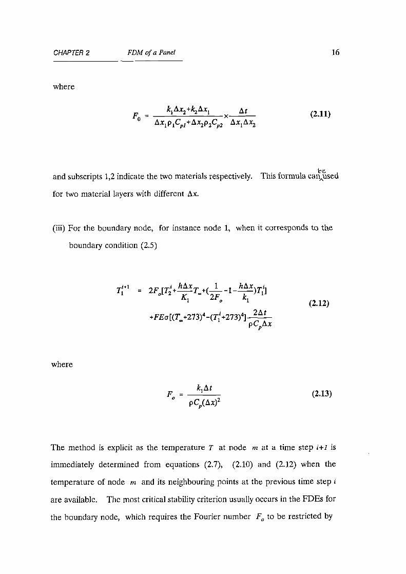
k1 Ax2 +k2 Ax 1 At F0 -
xAx1 p 1 Cp1 +Ax2 p2Cp2 AxiAx2
CHAPTER 2 FDM of a Panel 16
(2.11)
1.1e,
and subscripts 1,2 indicate the two materials respectively. This formula canAused
for two material layers with different Ax.
(iii) For the boundary node, for instance node 1, when it corresponds to the
boundary condition (2.5)
71 +1 = 2F0[T2i + —hAx T.+(-
1-1--
hAx)7.1
i]
K12F0 ki
+FEaRT.+273)4-(T:+273)4] 2A t
pCpAx
(2.12)
where
kiAtFo(2.13)
p Cp(Ax)2
The method is explicit as the temperature T at node m at a time step i+1 is
immediately determined from equations (2.7), (2.10) and (2.12) when the
temperature of node m and its neighbouring points at the previous time step i
are available. The most critical stability criterion usually occurs in the FDEs for
the boundary node, which requires the Fourier number Fo to be restricted by
CHAPTER 2 FDM of a Panel17
Fo s 0.5 [1 _,_ h Ax 4_ FEcy Ax . (T11+273)4
ki ki i l-1T1
(2.14)
In order to check the above treatment on the temperature -dependant thermal
properties of material, a typical test problem is solved. It is a designed problem
which has been used by some researchers to investigate an efficiency of numerical
methods for the solution of nonlinear transient heat conduction problems[2.2,2.3].
The question is to find the temperature distribution along the thickness of a wall
with temperature-dependent thermal conductivity. The wall is assumed to be
20cm long, lcm high, and is initially at 100°C. The temperature of the surface
of the left hand end is suddenly raised to 200°C and kept at this value for 10
second, after which it is decreased to 100°C again; the temperature of the surface
of the right hand end is kept at 100°C, while the other surfaces are presumed to
be insulated. The thermal conductivity is k = 2 + 0.01T W/cm°C and the
specific heat capacity is pC = 8 J/cm 3°C. Two available numerical results were
given by the relatively complicated FEM or BEM (Boundary Element Methods)
with an iteration process at each time step[2.2,2.3]. The time step for our finite
difference analysis is 1 sec and the length of wall is divided by 21 nodes. A
comparison of the results obtained using the three alternative numerical methods
is shown in Table 2.1. The values in the table are temperature distributions in
the wall at time t = 10 sec. The agreement between the results is very good.
This demonstrates that, although the explicit FDM is a simple algorithm, it is
also an effective method.

CHAPTER 2 FDM of a Panel 18
Table 2.1 Temperature distribution of the wall at time t = 10 s
x/(cm) FEM BEM FDM
0 200.00 200.00 200.00
1 176.16 175.29 176.36
2 153.21 151.48 153.50
3 133.47 131.74 133.68
4 118.60 117.63 118.69
5 108.98 108.94 108.95
6 103.72 104.27 103.64
7 101.29 102.01 101.22
8 100.37 100.97 100.32
9 100.08 100.50 100.06
10 100.01 100.27 100.01
2.3 Unexposed Side Heat Transfer Coefficient
In a general case, an insulating panel has an exposed side subjected to fire and
an unexposed side losing heat to an ambient environment. Radiation and
convection heat exchanges take place on both sides.
Convective heat transfer results in the movement of whole groups of molecules.
It is normally concerned with the heat exchange between a fluid and a solid

k.h(T)---- c —a-(G Pr
H rH r
(2.15)
CHAPTER 2 FDM of a Panel 19
surface. When the motion of the fluid is induced by buoyancy forces, such as a
hot panel in air, and where a change of density of air near the panel occurs due
to temperature increases, the mode of heat transfer is called free (or natural)
convection. When the motion of the fluid is externally induced, as with flowing
water in a pipe, which will be considered in next chapter, then although a small
amount of free convection may be present, the mode is called forced convection.
Since in standard test condition, only free convection is encountered on the
unexposed face, the calculation of its heat transfer coefficient is presented here.
For natural convection adjacent to a heated vertical or horizontal panel, the
following empirical formula applies [2.4]:
where for a vertical panel
c = 0.59 and n = 0.25 for 104 < G,.HP,. <109 ;
c = 0.10 and n = 0.33 for 109 < Gail', <i013.
kair is the conductivity of air which depends
on temperature: t
H is the height of vertical panel;
kair = -1.56x10⁻⁸T2 +7.43x10⁻⁵T+ 0.023 (2.16)
Gdi is the Grashof number defined as

CHAPTER 2 FDM of a Panel 20
gH3(T-T.)G - (2.17)rit
v2Tb
where
g is the acceleration due to gravity, 9.8m1s2;
Tb = (T T)12, is the average boundary layer absolute
temperature;
v is the kinematic viscosity of air:
V = 6.75x10 -6T2 + 9.55x10⁻³T+1.29 (2.18)
Pr is the Prandtl number of air which approximately
equals 0.7.
For the upper surface of a heated horizontal panel
c = 0.54 and n = 0.25 for 105 < Grip, <2x10⁷;
c = 0.15 and n = 0.33 for 2x10 7< Gri,Pr <1011.
In the above equation, the characteristic length L is defined as L = A/P, where
A is the surface area and P is the perimeter of panel.
The properties of air should be evaluated at the average boundary layer
temperature. The value of h(T) is increased as the difference between the
surface and environment temperature increases. A typical value is around 5
W1m2°C for a vertical panel with 300x300 mm 2 area.

CHAPTER 2 FDM of a Panel 21
When the heat transfer coefficient is known, the boundary condition (2.5) can be
applied to the unexposed side. The geometrical factor ( = 1.0 in most cases)
and the emissivity of the surface should also be determined.
2.4 Fire Boundary Conditions
Conventionally, fire can be classified as a 'Cellulosic' or 'Hydrocarbon' fire
depending on the type of fuel. The standard cellulosic fire test was developed
during the early part of the twentieth century and simulated the type of fire which
may be experienced in commercial, residential and general industrial construction,
while the fire which may occur in the petrochemical industry is appreciably
different. In the latter, the fuel is liquid or gaseous in nature. On the other
hand, the cellulosic type of fire is characteristic of a fire fuelled by solid
combustible materials which is generally in a contained space with limited air
movement. Specifiers in the hydrocarbon processing industry have long
recognised that the standard cellulosic fire test is less than effective in predicting
the performance of fire resistant materials in large scale hydrocarbon-fuelled fires.
Nevertheless, cellulosic fires should not be excluded offshore as cellulosic
materials are not insignificant, eg, within an accommodation module.
In actuality, there are many different fire scenarios that can occur in the real
world. For instance, hydrocarbon fires, which feature a very rapid initial
temperature increase together with fierce burning and a high release of heat flux,

CHAPTER 2 FDM of a Panel 22
in petrochemical industry may include:
. Jet fire: when a stream of fluids burns with some
significant momentum
•
Pool fire: when a spill of liquid fuel burns
. Running fire: a fire from a burning liquid fuel which
flows by gravity over surfaces.
Fireball or BLEVE: expanding buoyant ball of
flaming gas or a Boiling Liquid Expanding Vapour
Explosion caused by a catastrophic failure of a
pressure vessel containing liquid or gaseous fuel.
The duration of these different fire types can vary from seconds to days.
The standard fire has been adopted to unify test procedures and to enable
materials and construction elements to be compared and classified, although the
temperature development described by the currently standard time-temperature
curve does not necessarily agree with the temperature development experienced
in a real fire.
Currently, there are two basic types of time-temperature curve according to
BS476 and AMD 6487[1.1]:
1. Cellulosic time-temperature curve:
T = 345 1og10(8t+1) + 20 (2.19)

Hydrocarbon Curve
\
Cellulosic Curve
CHAPTER 2 FDM of a Panel 23
2. Hydrocarbon time-temperature curve:
T = 1100[ 1 - 0.345 EXP(-0.167 t)
- 0.204 EXP(-1.417 t)
- 0.471 EXP(-15.833 t) ]
where
(2.20)
T is the mean furnace temperature in (°C);
t is the time (in min) up to a maximum of 360 min.
The graphs of both curves are shown in Fig.2.1. During the first 170 minutes,
the defined hydrocarbon curve has a steeper rise and a higher fire temperature.
After 170 minutes, although the duration of most tests usually does not last so
long, the temperature given by cellulosic curve is higher than that given by the
Temperature (Deg C)
1 i 1 i I I 1 1 1 III
20 40 60 80 100 120 140 160 180 200 220 240 260Time In mins
Fig.2.1 The Standard Cellulosic andHydrocarbon Fire Test Curves 11.11
1400
1200
1000
800
600
400
200
hydrocarbon curve.

CHAPTER 2 FDM of a Panel 24
The expression (2.20) for the representative hydrocarbon fire test,
notwithstanding that it is not yet fully accepted by industry, is the most widely
recognized curve of this type.
The level of total heat flux could range from 35 KW/m 2 to 400 KW/m2 under
standard tests. Whilst a lot of researches have ignored the convective heat
transfer because the radiative heat flux is the dominant component of total heat
flux, it is not considered that this is a universally correct approach. For
engulfed conditions this may be a reasonable assumption. However, outside the
fire, the level of radiation drops away and the assumption becomes less valid. The
assumption is also less valid for surfaces that are highly reflective. As the
magnitude of the received radiation lowers, then the significance of convection
increases and convection may make a considerable difference to the fire
endurance of the element.
The heat transfer into a construction on the exposed side depends not only on the
temperature of the gas and flames but also on the heat transmission
characteristics of both the heating environment and the surface which is receiving
heat. The heat transfer and gas temperatures vary strongly during fire exposure.
As the phenomena associated with heat transfer in the turbulent environment of
a fire are difficult to model exactly, the following alternative schemes are
suggested:
i). Direct method: this measures the actual exposed face temperatures of
elements during fire test. These measured temperatures can be used in
two ways. One is that they can be applied as the Dirichlet boundary

CHAPTER 2 FDM of a Panel 25
condition (2.4) in numerical modelling. This excludes the uncertainties
with regard to the parameters describing the heat transmission from the
furnace to the specimens. In the experimental validations of this
research, this method is used first to examine the numerical model.
Secondly, it can also be used to validate the heat transfer parameters (see
following ii).
ii). Heat transfer parameters: although the exact modelling of the heat transfer
from fire to specimen is extremely difficult, eventual consideration should
be given to the possibility of including the appropriate heat transfer
parameters to predict the heat transfer rate from the fire to the specimen.
The heat transfer rate from the fire compartment to the panel could be
described as a boundary condition using equation (2.5). Here T., should
be assumed to be the mean furnace temperature, and E represents the
resultant emissivity. The resultant emissivity could be calculated
approximately with the equation for radiation between two infinitely large
parallel planes[2.4], so that:
E- 1
11E1+11E5 - 1
where
Ef is the emissivity of gases, flames and walls in furnace;
Es is the emissivity of surface material of specimen.
(2.21)
Ef should be experimentally determined for the furnace. Since this experiment

CHAPTER 2 FDM of a Panel 26
for the furnaces used in the tests has not been performed, an estimate is made
which is based on an educated assumption and a series of calculations. Usually
the both the emissivities of the furnace and the heat transfer coefficient are
assumed to be constants[2.5]. A considerable error was encountered if this
assumption was adopted for the gas-fired furnaces. It was found that the both
emissivities of furnace and the heat transfer coefficient should be high at the
starting stage, and that they then declined as the temperature increased. The
declining trend of Ef is consistent with the research results on the emissivity of
gas[2.6], insulating brick[2.7] and ceramic fibre linings[2.8]. For the convective
heat transfer coefficient, the reason for the decline is that, at the starting stage
of a test, the temperature of the furnace is increased very quickly so that the
extent of fire turbulence is high at first.
In the environment of the furnace used for Cellulosic fire test, it is assumed that
.E1 = 0.9 at the beginning of the testing and then linearly declines to Ef = 0.15.
The average of both values is close to the conventional value of 0.5. The -. ,
heat transfer coefficient is h1 = 60 WIm 2 °C at beginning of the test and this
decreases to h2 = 2 WIm2 °C at 1000°C. The numerical results based on these
parameters give a good correlation with experimental results(see Chapter 6).
For hydrocarbon fires, similar results can be obtained. The slight difference is
that at initial stage, the heat transfer coefficient should be higher than with a
cellulosic fire.
The experimental verification of the aforementioned formulas will be described
in the subsequent chapters.

27
CHAPTER 3
Finite Difference Modelling of a Pipe
Another extensively used component of construction in onshore and offshore
constructions is pipework. A cylindrical polar coordinate model is needed for the
heat transfer analysis of pipes under hostile thermal impact. Usually the heat
loading is around the outside of the pipe and the following analysis is based on
this assumption. Only a slight modification is needed to deal with the reverse
case, i.e., heat loading from the inside of a pipe, such as the chimney problem.
3.1 1-D Explicit Formulation of FDM for a Multi-layer Pipe
Assuming that the pipe is subject to a uniform heating condition and that the heat
transfer occurs only in the radial direction of the pipe, the general one
dimensional heat conduction equation can be written as:
pC —aT = —1-5
(07)r—OT
) in Ri �rs1?2, for t>0P at r ar ar
(3.1)

28
where
r is the polar coordinate.
kris the thermal conductivity in the radial direction.
RpR2 are the inside and outside radii respectively.
The boundary and initial conditions are similar to equations (2.4), (2.5) and (2.6).
The boundary condition on r=R i or r=R2 for t>0, is either:
T = Tg(t) (3.2)
where Tg (t) is the known temperature given on the inside boundary or outside
boundary; Or, if the boundary is losing heat to or gaining heat from an ambient
temperature condition:
c7Tk(7)— = h(7)(To.-7) + FEaHT.,+273) 4 -(T+273)4] (3.3)
an
The initial boundary condition is:
T = To(r)
for t = 0 in R1 srsR2(3.4)
where To is the known initial temperature distribution.
The appropriate explicit finite difference equations for a multi-layer pipe can also
be obtained by the energy balance technique. The advantages offered by the use

CHAPTER 3 FDM of a Pipe 29
of sandwich design in pipelines include enhanced insulation capability, double
integrity containment and leak or failure protection. The problem requires four
different types of FDE to be derived:
a) the interior nodes within one material layer;
b) the interface nodes between two material layers;
c) the external boundary node;
d) the internal boundary node.
(a) For an interior node m within one layer:
Ti #1 = T i + 1-*2 "1+m Or2
+ km _i,m(r„,-1)(Tni,
The evaluation of the conductivity k„,_ /,„, or km+im is same as in equation(2.9).
The Fourier number is
[kmn"
i (r /Or ÷0.5 ) + -1,m(r „, /Or -0.5)7 dtF- '
2PCpTmÔT
(3.5)
(3.6)
(b) For the interface node m between two material layers

CHAPTER 3 FDM of a Pipe 30
T.1+1 = 7' 1 + At
p Spi(rni -Ori/4)6r 1/2 +p2Cp2(r.+6r2/4)6r2 /2 .1-k"+1
(r„, /6r2 +0.5)(Tm1 #1-T,;)+1c._4.(r„, gr1 -0.5)(Tml _1-7;)]
The Fourier number is now
F =min+i(rm /6r2 +0.5) +km _i,m(rm /Or, -0.5) At
° p Spi(rm -Or /4)Sr + p2Cp2(r.+6r2 /4)6r2
where subscripts 1,2 indicate the two materials respectively.
(c) For the outside boundary node m:
Tmi #1 Tin + At [km_im(r. / Or -0.5)(T.1pC p(r.-6r/4) 6r/2. '
(3.7)
(3.8)
(3.9)
h(T)r.(Tfire -t) + FE ard(Tfire +273)4 -(t +273)4)]
where Tfire is the furnace temperature. The Fourier number is
(m
rm /Or -0.5) +hr m +FE arm(Tm +273)4/Tm] At
F - nimpCp(r.-6r/4)Sr
(3.10)
These Fo 's should be less than 0.5 in order to preserve the stability of the

CHAPTER 3 FDM of a Pipe 31
calculation.
(d) For the inside surface node 1:
Tii #1 = + 2 At fki 2 (ri + 0.5 Or)(T2i -7'1) +hr Or(Ta -Td] (3.11)
pCp(ri +0.2. 5 Or)(Or)2
where is inside heat transfer coefficient
Ta is the temperature of inner flow
3.2 2-D Explicit Formulation of FDM for a Multi-layer Pipe
When the heat loading is no longer uniform along the circumferential direction
of a pipe, the problem becomes two dimensional. In this case, the general two-
dimensional heat conduction equation can be written as:
r, 87' 1 8 ,n r,,,, 8T, 1 8 „e,,„ OT--i , ( A 1-1
-a r r 2 09 80(3.12)
in R1 r R 2 , 0 0 27r
where
r,0 are the polar coordinates;
CHAPTER 3 FDM of a Pipe 32
kr is the thermal conductivity in the radial direction;
ke is the thermal conductivity in the circumferential direction;
R1 ,R2 are the inside and outside radii respectively.
The boundary and initial conditions are similar to equations (3.2),(3.3) and (3.4).
There are four different types of FDE to be derived as well:
a) the interior nodes within one material layer;
b) the interface nodes between two material layers;
c) the external boundary nodes;
d) the internal boundary nodes.
(a) For the interior nodes within one material layer:
T' = AtT. + 40(ri +0.5)(Ti+m-Tin)
41 pCg
r.drA0 ArP
ri
LIT+ A 0(— • k°..;„_1;,
" dr "" "'ride
(Tij-1 -7i) ÷ ki.ewq)
Arrede(Tii+l-Tu)]
where a prime ' denotes the temperature at next time step.
(b) For the interface nodes between two material layers
(3.13)
CHAPTER 3 FDM of a Pipe 33
u = T1, + 2 At pnC pn(r L -0.25 Ar ft)Ar n + pn+IC;+1
r.(ri +0.25 Ar n+1)Ar"1] A 0) -1 f Ic(27.1) .A 6( g +0.5)(T. )+1 —Tij
Arn+1
r.+ k r'n A 0(-.—0.5)(T. —7)1-1j
AT n
• an Ar n +k"+I Arn+jiTijJ ÷I) i,Cij +1) • 1
+ (Ic e' n Ar n +ic on +1 A n#1 (Tii -1 —7; ) 4u-4D r ) ]
2ri A 0
2riA 0
(3.14)
where the superscripts n,n+1 indicate materials.
(c) For nodes on the inside surface:
T' . = T 2 At 0(1-:fe ' r +0.5) •kzI
1J pC p(r +0.25 Ar) A r A 6 '
(T2j-7i) + kie(_ij) 2r
AAr 0(7,
11. _7
I • ke
J-) 4_
1,(ij +1)1
Ar (Ti . #1 -7.1 ) + r 1 7A 012r I A 6 '1
(3.15)
where 7 is the unit net heat flux due to radiation and convection. The
evaluation of 7 will be presented in section 3.3.
(d) For outside boundary nodes:

e heat capacity of air can be neglected due to the small mass of airI IIwith air,
CHAPTER 3
TDM of a Pipe 34
2A1 r ,ru =
pC Jr.-02511r) kt(r1414141A 9( r —.au/
keoj „,i) A r -Tij)2ir
ka4-1.42reir 4j-1 2riA 0 4+1
hifirgitifTfre-Td FaerKA OffTfire -1-273)4 -(T +273)4 )1
(3.16)
33 Internal Heat Exchange
For one-dimensional analysis, if the inside of pipe is empty, eg, the pipe is filled
inside. If the pope is filled with flowing water, forced convective heat dissipation
is encoomtered. For a flow inside a circular tube, the rate of heat transfer
depends on e type of flow, le, laminar or turbulent flow. When the flow
through ii ye pipe is stre mlined and in consequence little mixing takes place, the
heat transfer is relatnely poor. When the flow becomes turbulent and there is
very rapid mixing action, much higher convection rates then take place.
The Reynolds number, defined as Re = un, D v is used as a criterion for defining
the chance from laminar to turbulent flow[3.1]. In this definition, Urn is the mean
flow velocity, D is the inside diameter of pipe, and V is the kinematic viscosity

e heat capacity of air can be neglected due to the small mass of airIwith air,
CHAPTER 3
FDAI of a Pipe 34
Zit-
14.11
= T - kr .11,A -0.5)(Ti 4-Ti.j)pC'p(r.-0.25 Ar) Ar A 0 141 - Ar
k .) Ar (T. .Ar4'4 ZriAr (14.1) 2r ill 0 4+1
(3.16)
h(T)rgiO(Tfre -Tv) FacriA Oarfire +273)4 -(Tij+273)411
33 Internal Beat Exchange
For one-dimensional analysis, if the inside of pipe is empty, eg, the pipe is filled
inside. If the pipe is in ied with flowing water, forced convective heat dissipation
is encountered_ For a flow inside a circular tube, the rate of heat transfer
depends on e type of flow, ie, laminar or turbulent flow. When the flow
through , oe pipe is streamlined and in consequence little mixing takes place, the
heat transfer is relatively poor. When the flow becomes turbulent and there is
very rapid mixing action, much higher convection rates then take place.
The Reynolds number, defined as Re = un, D v is used as a criterion for defining
the change from laminar to turbulent flow[3.1]. In this definition, um is the mean
flow velocity, D is the inside diameter of pipe, and V is the kinematic viscosity

CHAPTER 3 FDM of a Pipe 35
of the fluid. The range of Re value in the transition stage is around 2000 Re <
4000. Since in most practical cases the values of Re are greater than 4000,
turbulent flow inside the pipe is assumed. The empirical formula which was
proposed by Nusselt is employed to calculate the internal heat transfer coefficient
h(T)[ 2. 4 ] :
h(7) = 0.036ReasPrifi(D/4"551- for 10<—L <400D
(3.17)
where
L is the length of the pipe;
D is the inside diameter of the pipe;
k is the conductivity of the fluid;
Pr is the Prandfl number of the fluid.
The fluid properties are evaluated at the bulk mean fluid temperature. A typical
illustration of the influence of fluid speed on the inside temperature rise in a GRP
pipe under the standard hydrocarbon fire test is shown in Fig.3.1.
If the pipe is filled with stagnant water, the problem will be more complicated
because a mixture of conduction and convection occurs. At low temperature, the
heat transfer through the water may be considered to be by conduction only,
while, as the water temperature increases rapidly in a fire environment,
convection will occur.
For the two dimensional analysis of an empty pipe, the heat exchange between

qc = fi(Ti - T . )7 (3.18)
CHAPTER 3 FDM of a Pipe 36
the different parts of the inside surface should be taken into account. Although
many construction components and assemblies enclose voids, no general
procedure which may be used to calculate heat exchange by radiation and
convection through a void has been available[3.2]. Thus some simplifying
assumptions are normally needed. One of these is to consider the conduction
and specific heat of the internal air to be negligible. The inside curved surface
is replaced by a finite number of discrete straight zones. The convective heat
transfer to an enclosure boundary is written as
where
13,y are the convection factor and convection power;
Tiis the surface temperature of the zones;
Tair is the fictitious inner air temperature.
The air temperature is assumed to be uniform over the inside of the void and
there is presumed to be no flow of air either in or out of the void. The total heat
transfer to the air from the enclosure surfaces must be zero at any given time in
order to conserve the energy. The total heat transfer to the enclosed air is
N
=' qc, Ai = 0i 4
where
N is the number of zones;
Cid is the heat flux per unit area;
zirc, (3.19)

CHAPTER 3 FDM of a Pipe 37
is the area of zone i.
If all of the temperatures T i are known, Tair can readily be computed by iteration
and the local heat transfer to zone i can be calculated.
Regarding radiation, only diffuse-grey surfaces are considered. This means that
the directional spectral emissivity and absorptivity do not depend on either angle
or wavelength, but only on surface temperature. Although most materials are
not truly diffuse-grey, this assumption simplifies enclosure radiation theory and
is often made. The inside surface of the pipe is divided into a number of zones.
The temperature and heat flux of each zone are assumed to be uniform. The
Hottel's crossed-string method[3.3] may then be employed to calculate view
factors for the two-dimensional configuration. Radiation heat flow and absolute
surface temperature for an enclosure with N zones can be related by the following
expression[3.4]
N -e. 111, N
Z(-41 - 1
= E(Fki - (5k) cal=1 5 e A •I j =1
(3.20)
where, corresponding to each zone surrounding the enclosure, k is one of the
values 1,2,...,N, Trj is radiative heat transfer, Fkj are view factors and S ki is the
Kroneker delta. When the surface temperatures are specified, the right hand
side of Eq.(3.20) is known and there are N simultaneous equations for the
unknown Tr The sum of 'P c and Tr will be the required T in the Eq.(3.15).

140
120
100
80
60
40
20
0
CHAPTER 3 FDM of a Pipe 38
Temperature (Deg C)
o 3
6 9
12
15Time in mins
Fig.3.1 Inside Surface Temperature Risein a GRP Pipe (5mm) with Flowing WaterHydrocarbon Fire, Computer simulations

39
CHAPTER 4
Models for Polymeric Composites
4.1 Introduction
The use of fibre reinforced polymer composites, and in particular Glass-fibre
Reinforced Plastics (GRP), is increasing now owing to their inherent advantages
in material characteristics, such as good corrosion resistance, low weight and
cost, long service life and low thermal conductivity, typically 1/10Dof steel.
However, because plastic materials are organic in nature and are inherently
combustible, one of the key problems which needs to be overcome before they
are accepted for wider use relates to the need for improved understanding and
quantitative evaluation of their behaviour in fire. Accurate knowledge of the
thermal response of GRP at high temperature is therefore essential for the
reliable and economical design of composite structures in hostile fire environments
such as may be encountered on offshore oil platforms.
Let us look at what will happen when a typical GRP panel is exposed to fire.
When one surface of the GRP panel is exposed to an incident heat flux, the
initial temperature rise is a function of the rate of heat conduction into the
material and the boundary conditions. As heating continues, the surface

CHAPTER 4 Models for Polymeric Composites 40
temperature reaches a certain level (usually around 200-300°C) beyond which
decomposition begins to occur and the resin components degrade to form gaseous
products at a measurable rate. These gaseous products, initially trapped within
the composite matrix owing to its low permeability, attain very high internal
pressures and induce the solid matrix to expand. Once the decomposition
process begins, the thermal behaviour of the material is altered by the chemical
reactions, thermochemical expansion and variable thermal and transport
properties. Meanwhile, a considerable amount energy will be required in order
to break the constituent chemical bonds. As thermal decomposition proceeds,
a residual char layer then builds up as the pyrolysis front moves further into the
virgin solid. An advantage of thermosetting resins (which are generally used in
GRP) is that usually they do not melt when heated owing to their highly cross-
linked chemical structures. Initially, the char layer provides an increasing
thermal resistance between the exposed surface and the pyrolysis front as a
consequence of its low thermal conductivity and because it can only be ignited
with difficulty at normal oxygen concentrations. This is the one reason why GRP
can provide a useful fire barrier performance, despite it being an organic
material. However, after this initial phase, at a certain stage in the heating
process, a network of fissures develops in the carbonaceous char layer due to the
release of high pressure gasses. At very high temperature, the char is then
gradually oxidized and erodes away. Then the heat resistance of char layer will
be totally lost and the glass-fibre remains alone. Under extremely strong heat
flux, such as is experienced in a hydrocarbon fire, even the woven roving glass
plies will crimp and eventually crumble away.
t"5
This problem , some differences with the ablation problem experienced in the
CHAPTER 4 Models for Polymeric Composites 41
isaerospace industry, which,usually associated with rocket nozzles or missile reentry
situations. Their major concern is the total energy which must be absorbed into
the surface body rather than a heat transfer rate. Another consideration is that
in their situation, a portion of surface body exposed to the hot, high speed fluid
flow is allowed to melt and rapidly blow away.
Over the past 50 years, several analytical models have been proposed which
consider heat transfer in decomposing materials [4.1 to 4.9]. All of these
procedures were basically a transient heat conduction calculation in conjunction
with the effect of decomposition. The differences existed in their assumptions,
approximations, the phenomena included and the property data used. Although
most of these studies were concentrated on wood, they provided a theoretical
basis for further investigation of the fire performance of other combustible
materials.
There are two basic ways to tackle the decomposition of material implicit and
explicit approaches. The implicit methods[4.4,4.9] include the effects of
decomposition by artificially increasing the specific heat for the temperature range
in which pyrolysis occurs. The author does not think that this is very appropriate
for such a complex problem. The comprehensive explicit methods[4.3,4.6,4.8]
model the decomposition as an exponential kinetic rate equation. The
conservation of mass and heat of reaction are therefore included. The diffusion
of volatiles is also considered. It is believed that this is a better approach.
Arising from the mathematical models proposed by Kung[4.3], Henderson et
a/[4.6,4.8] presented a numerical model for the thermal response of polymer
CHAPTER 4 Models for Polymeric Composites 42
composite materials together with an experimental verification. Most of the
essential processes relating to the temperature development in the process of
decomposition were included in the model. But, probably because of the test
assembly used, the fact that only a relatively low constant heat flux was imposed,
and due to the particular material used in their test, the profile of measured rate
of increase of temperature did not display as much variation as we have observed
in standard fire testing of GRP panels.
In this study, the solution of a more realistic problem is attempted, namely that
of a glass-fibre reinforced plastic panel and pipe exposed to the time-temperature
regime of a standard fire test. For the associated tests, the furnace temperature
was controlled by computer to follow the standard BS476 cellulosic fire or
hydrocarbon time-temperature curve 1.11.
The fire tests revealed that if the empty GRP pipes were exposed directly to a
hydrocarbon fire, they can only survive for a few minutes. Therefore it is
necessary to add additional protection to the plain GRP pipes. One method is to
use a polymer based flame-retardant intumescent coating.
In a fire, an intumescent coating undergoes several chemical changes in order to
act as a thermal barrier between the heat source and the substrate. Generically,
three main ingredients are necessary for this process: a catalyst, a carbonic (char-
former), and a spumific(blowing agent). The catalyst promotes decomposition
of the carbonific compound. Initially, an inert gas is liberated to provide
transpirational cooling at the surface. As the fire continues, other ingredients of
intumescence break down, expand and absorb heat. A low density carbonaceous

CHAPTER 4 Models for Polymeric Composites 43
char then forms and this is expanded by the spumific agent which provides a good
insulating blanket due to its low thermal conductivity. These reactions combine
to make intumescent coatings into a most efficient fireproofing material although
the labour involved and cost are relatively high.
To date, only a few mathematical models have been based on the fundamental
chemical or physical processes occurring in a complex intumescent coating system
such as heat transfer, kinetics, and swelling[4.10 to 14]. The various physical
processes were considered in mass and energy control volumes. Expansion has
been accounted for by assuming it to be a function of mass loss.
theWith the combination of„above models and the treatment which was originally
developed by J.B.Henderson and T.E.Wiecek[4.8] to predict the thermal response
of a polymer composite simultaneously undergoing decomposition and
thermochemical expansion, an analysis of the heat transfer problem associated
with intumescent coatings under hydrocarbon fire is carried out in this paper.
The accuracy of the model was evaluated by comparing predicted and
experimental temperature distributions in the intumescent coated GRP pipes.
4.2. Model for WR Polyester Laminate
The first GRP component to be used for the experimental and numerical fire
resistance study was
the woven roving glass-fibre reinforced polyester laminate.
Because of their low cost, ease of processing and good performance

11I I I I I I
CHAPTER 4 Models for Polymeric Composites 44
characteristics, unsaturated polyesters are the most extensively used type of
thermosetting resin. Woven Roving (WR) cloth is a popular fabric to produce
high directional strength characteristics. Bidirectional roving cloth laminate,
which was used in the present study, has high strength properties in two
directions at right angles to each other. The WR glass/polyester laminates were
made using a hand lay-up technique with a ply angle of zero. The thini i il 4. r eruc t ›) )
thermocouples (K type) were embedded insiore the central area at different
locations to measure the temperature profile history across the cross-section of the
laminates (Fig.4.1).
6 5 4321
Fig.4.1 The layout of laminate and the location of thermocouples
Since the physical and chemical processes are concurrent, the problem of
interpreting and predicting the observed results is a task of awesome complexity.
It is considered that main task at . present is not to attempt to form a
'complete' model owing to the almost total absence of information concerning

CHAPTER 4 Models for Polymeric Composites 45
most of the material parameters involved. The most promising approach is to
form a mathematically viable but relatively simple model which can capture the
main features of the pyrolysis process and the consequent heat transfer behaviour.
Therefore, several idealizations are made:
a). The GRP material is assumed to be homogeneous and the
transport of heat and mass is perpendicular to the face of panel so
that the problem is assumed to be one dimensional.
b). The rate of decomposition is assumed to conform to a mean
reaction which is described by a single first-order Arrhenius
function.
c). There is thermal equilibrium between the decomposition gases and
the solid material and there is no accumulation of these volatile
gases in the solid material.
d). The feedback of heat released by the flame of the combustible
volatile back to the panel in a small scale furnace test is neglected
owing to its relatively small contribution compared with the
enormous heat flux created by the furnace. However, it is
anticipated that in large or full scale fire tests, or in the case of
sustained combustion after removal of the heat source, its
contribution may not be ignored.
The governing principles on which the analytical model has been developed are
a combination of the principles of conservation of mass and conservation of
energy. The one-dimensional energy equation in a panel undergoing thermal

CHAPTER 4 Models for Polymeric Composites 46
decomposition expresses a balance between the transient energy accumulation
rate, with the sum of the rates of conduction, pyrolysed convection, and the
energy sink due to decomposition[4.6]
8 Op-L3 (ph) =—(k—)
81' -
0—(m
, g hg) -Q aa & dc c7x
where
p is density (kg/m3)
h is the enthalpy (J/kg) of i.50 icL
t is time (s)
T is the temperature (°C)
k is the thermal conductivity (W/m°C)
x is the spatial variable (m)
hgis the enthalpy of gas(J/kg)
m ' g is the mass flux of gas (kg/m2-s)
Q is the heat of decomposition (J/kg)
The specific enthalpies of the solid and volatile are
h = r
CpdT , hg = fr_ CpgdT (4.2)ToTo
(4.1)
where T. is the ambient reference temperature.
Equation (4.1) must be solved simultaneously with the equations for the rate of
decomposition and the mass flux of the gas. The rate of decomposition of resin

CHAPTER 4 Models for Polymeric Composites 47
in GRP is assumed to conform to a mean reaction which is described by a single
first-order Arrhenius function
dp,dt - -A prexp(-EA/R7)
where p r is the instantaneous density of partially pyrolysed resin, EA is the
activation energy (J/mol), R is the gas constant (8.314J/K.mol) and T is the
temperature (K). The constant A is known as the pre-exponential factor and has
unit of s -1 . The relationship between the p and p r is:
p = prv + p g (1 -v)
(4.4)
where p g is the density of glass-fibre and v is the volume fraction of glass-fibre.
The glass-fibre is assumed to be intact in the time zone of interest under fire.
Here, the resin pyrolysis is assumed to be a continuous process until it is totally
consumed. Some investigators have included the final density of the char in the
expression (4.3). This will cause two problems in practical application. One is
that the precise definition of the final char status is difficult to define. Another
point is that yet another expression for char pyrolysis will be then required if it
commences its final breakdown in the time zone of interest. Although much
research has been carried out into the thermal decomposition of polymers, in
view of the chemical complexity involved, combined with problems of interpreting
data from a variety of sources and experimental assemblies, the available data is
still very limited and not in a form suitable for warranting improvements to the
(4.3)

am'g op (4.5)
CHAPTER 4 Models for Po lymeric Composites 48
above relatively simple treatment.
Another facet which shows the complexity of the problem is the determination of
the heat of decomposition (sometimes called the heat of pyrolysis or heat of
reaction). It was reported that its value for wood, for instance, varies
greatly[4.15]; and that not only the magnitude but the actual sign of this property
has been the subject of debate for many years[4.16,4.17]. We prefer the
allegation which declares that the decomposition process itself is endothermic
overall. The exothermicity often noticed in the burning of wood and plastics is
a result of the reaction between the outflowing volatiles and oxygen. A minor
exothermic reaction might happen within the extremely complicated competing
reactions, or a local exothermic phenomenon appears due to the change of
specific heat. However, in most circumstances, the endothermic reaction is
believed to be dominant in the decomposing process for polymeric materials.
If the accumulation of gases and the effect of expansion on density change are
ignored, the conservation of mass may be written as:
and the mass flux, m , g , at any spatial location and time can be calculated by
integration of Equation (4.5).
Equation (4.1) is modified to its final form by expanding the first three terms,
substituting in the specific heat and the continuity equation, and rearranging.
This results in[4.6]

CHAPTER 4
Models for Polymeric Composites 49
OT 82T c aT -!9. 12(Q, +h -hg )pC = k-4-2,c2 m g pg
where
is the specific heat of material (J/kg°C);
is the specific heat of gas (J/kg°C).Pg
Equations (4.3), (4.5) and (4.6) form a set of non-linear partial differential
equations which may be solved simultaneously for p, m ' g and T respectively.
The boundary conditions on the exposed and unexposed surfaces of a panel could
be either a prescribed temperature or a radiation and convection boundary
condition. To exclude the uncertainties of the heat transmission rate from the
fire to the samples under test, the measured temperature can be used as the
boundary condition at the exposed side. On the unexposed side, equation (2.5)
is again applied.
The initial conditions for 0 x L at t = 0 are
=Ti ; p = po ; m'g =0. (4.7)
where
Ti is the initial temperature (°C);
p 0 is the initial density (kg/m3).
(4.6)
The comparison of the measured and calculated results shows a good correlation
(see Chapter 6). It is shown that the above scheme can be straightforward to

6 5 4.4' 2,3' 2 1
1
1
i
1 1 II 1 1 1 1 I 1
1 1 I II I I I I I I1 I II I I I I I I1 I I I I I I I 1
1 I II I I I I I I
/I 11111111/
1
1 1
1 1
1 1i
1 11 1 1 .W
in
CHAPTER 4 Models for Polymeric Composites 50
apply to the epoxy and vinyl ester systems. However, for phenolic resin
laminates, a more complex behaviour was observed. This requires a special
treatment which will be discussed in the next section.
4.3 Special Treatment for WR Phenolic Laminate
Phenolic (phenol-formaldehyde) resins, whose development was once superseded
by that of polyesters and epoxies, have experienced a recent recovery in
popularity which is mainly attributable to their good fire resistance and low smoke
emission (about 10% that of polyester-based GRP).
The test samples of woven roving glass/phenolic laminate were made in a similar
manner to the WR polyester laminates as shown in Fig.4.2.
Fig.4.2 The Phenolic laminate with the location of the thermocouples
1200Hydrocarbon Curve4 Ave' Furnace Tame
Cold Face Tema..
1000
800
600
400
200
CHAPTER 4 Models for Polymeric Composites 51
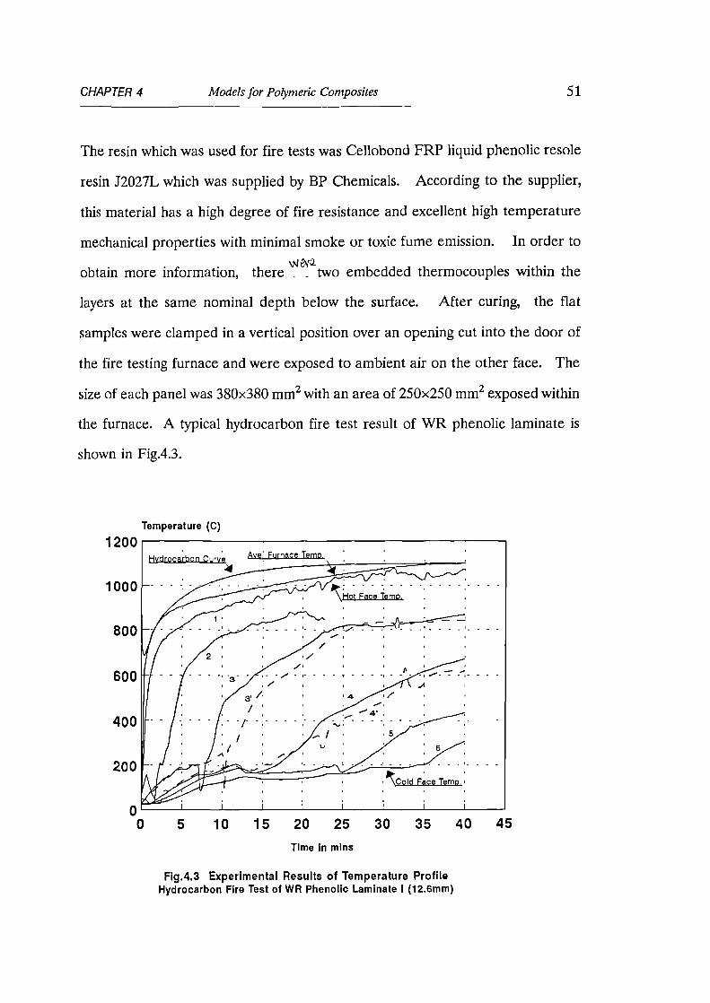
The resin which was used for fire tests was Cellobond FRP liquid phenolic resole
resin J2027L which was supplied by BP Chemicals. According to the supplier,
this material has a high degree of fire resistance and excellent high temperature
mechanical properties with minimal smoke or toxic fume emission. In order to
\Nevaobtain more information, there _ two embedded thermocouples within the
layers at the same nominal depth below the surface. After curing, the flat
samples were clamped in a vertical position over an opening cut into the door of
the fire testing furnace and were exposed to ambient air on the other face. The
size of each panel was 380x380 mm 2 with an area of 250x250 mm2 exposed within
the furnace. A typical hydrocarbon fire test result of WR phenolic laminate is
shown in Fig.4.3.
Temperature (C)
5 10 15 20 25 30 35 40 45Time in mins
Fig.4.3 Experimental Results of Temperature ProfileHydrocarbon Fire Test of WR Phenolic Laminate I (12.6mm)

CHAPTER 4
Models for Polymeric Composites 52
A first impression of Fig.4.3 suggests that the temperature response inside the
phenolic laminate was quite erratic. In the initial stages of the test, the
temperature rose at a moderate rate. Then, at about 200°C, there was a
sudden drop of temperature at most locations. After this sudden drop, the
temperature at each location concerned increased rapidly again. It was found
that this unusual behaviour is due to the delamination of the laminate.
Consider, for example, the output of measured temperature given by two
thermocouples at position 3 (see Figs.4.2 and 4.3, where 3 and 3' refer to two
different thermocouples in the same layer). Before the temperature reaches
200°C, both thermocouples indicated almost identical temperature values. Then,
at 200°C, the reading of one thermocouple suddenly dropped to 80°C. This
indicates that the cooler air was drawn into the interstice when a delamination
abruptly occurred. After delamination, the outcome of measured temperature
will be strongly dependent on the location of the thermocouple which introduces
a random element into the measurements. As illustrated by Fig.4.4, if the
thermocouple is attached to the surface B, its reading will be high. If the
thermocouple is attached to the surface B', its reading will be low. Evidently,
if the thermocouple is remote from the region of delamination, an intermediate
reading will be obtained. Furthermore, in volatile turbulence, the reading
given by a thermocouple in the region of a delamination is unlikely to remain
completely stable. This is illustrated by curve 4' in Fig.4.3.
The delamination is also demonstrated by observations made during the progress
of the tests. A lot of loud 'bang' sounds were heard which emanated from the
laminate during the fire test. This violent delamination is believed to be caused

CHAPTER 4
Models for Polymeric Composites 53
by the vaporization of intrinsic water (by-product of polymerisation[4.18]) in the
resin over 100°C. The water vapour, initially trapped within the composite
matrix owing to its low permeability, attains very high internal pressures as
heating continues. At about 200°C, a sudden release of high pressure tears the
laminate. A subsequent examination of the tested sample also reveals the
appearance of deaminations.
B A
Fig.4.4 Heat transmission through a delaminated surface
Although delamination causes a detrimental effect on the structural integrity of
the laminate, it may be beneficial in term of heat resistance as shown by cold
face temperature curve 6 in Fig.4.3. Due to the creation of a delamination in the
hotter part of the laminate, the mechanism of heat transfer from the hot side to
the cold side will be altered. Before the appearance of a delamination, the
internal heat transmission is mainly by conduction, whereas, within the interstice
caused by the delamination, radiation and convection will be dominant. Initially,
for example at point B' in Fig 4.4, the amount of heat transferred by radiation
and convection will be lower than that transferred by conduction. Then,
following the appearance of a discontinuity in the heat conduction path, the

CHAPTER 4 Models for Polymeric Composites 54
temperature at that point declines. It is clear that the heat transfer by conduction
is disturbed by delamination. This is one of reasons why the cold face
temperature of WR phenolic laminate can remain at a low and fluctuating level
for quite a long time. Another reason is the energy sink caused by the
decomposition of the resin as described for polyester resin in the previous section.
The fundamental equations for this problem are the same as those formulated in
section 4.2. However, a particular heat transmission equation will now be
established for the delaminated interfaces.
As shown in Fig.4.4, it is assumed that the layer AB is detached from the main
body of the laminate. Then an additional term should be included in the energy
conservative equation for points B and B' to take account of the heat transmission
by radiation and convection between B and B'. If these are assumed to be on
two infinitely large flat surfaces, the equation for the magnitude of heat flow G
is
G = Era I(T B 4-273)4 - (TB /+273)4] + H (TB -TB!)
(4.8)
where
Er is the resultant emissivity;
H is the heat transfer coefficient.
On the right hand side of equation (4.8), the first term represents the radiation
and second term represents convection.
Since both the theoretical prediction and the explicit experimental measurement

CHAPTER 4 Models for Polymeric Composites 55
of above two parameters are difficult, they are determined by finding a
reasonable fit between the model and the observed results. In the final analyses,
Er is set as 0.9 and H is given the value 20 WPC. It is found that the radiation
energy provides the major component of G.
By introducing this equation, a good agreement between the experimental and
computational results was obtained (see chapter 6). It demonstrates that a good
explanation has been given for the bewildering outcome of the measured
temperature development in WR glass/phenolic laminate in a fire.
4.4 Model to Predict the Thermal Response of GRP Pipes
In the offshore industry, it is necessary to design key components of the
installation to withstand the effects of fire. One such component is the fire-water
system which supplies a deluge of water in the event of a fire-related emergency.
Traditionally, fire-water systems have used steel pipework but there is
considerable interest in replacing steel with GRP because of its corrosion
resistance and lighter weight[4.19]. In order to prove the viability of GRP dry
riser pipes in this context, it is necessary to demonstrate that they can withstand
the effect of the fire on the empty pipe until the pipe is full of water and the
deluge system is in operation.
This problem has been approached by a combination of fire testing and numerical

CHAPTER 4 Models for Polymeric Composites 56
analysis. A one-dimensional analytical model for GRP pipes subjected to avn1 as
prescribed time-temperature history applied by the furnace developed. ThevJa.s
explicit finite difference method employed to solve the transient heat conduction
equation in polar coordinates. The performance of GRP pipes under fire
condition is quite similar to that of GRP laminates. The two possible differences
could be
1. Although some blisters may be observed on the inside of the pipe
at the final stage of a fire test, wholesale delamination in GRP
pipes can not happen because the glass-fibre reinforcement is
wound helically into the cylindric shape.
2. The loss of heat from the cold face, i.e., the inside of pipe, is
restricted in the empty pipe. This means that the temperature
increase in the pipe will be more rapid.
The fundamental assumptions and principles described in above sections are still
applicable for pipe problems. The only thing that is required is to recast the
equations in a polar coordinate system. The transport of heat and mass is
assumed to be only in the radial direction of the cross-section.
Using the same principles that were used with the polymeric composite panels,
an analytical model for the pipe problem is developed. The one-dimensional
energy equation in a pipe undergoing thermal decomposition, expressed as a
balance between the transient energy accumulation rates, with the sum of the
rates of conduction, pyrolysed convection, • and the energy sink due to pyrolysis
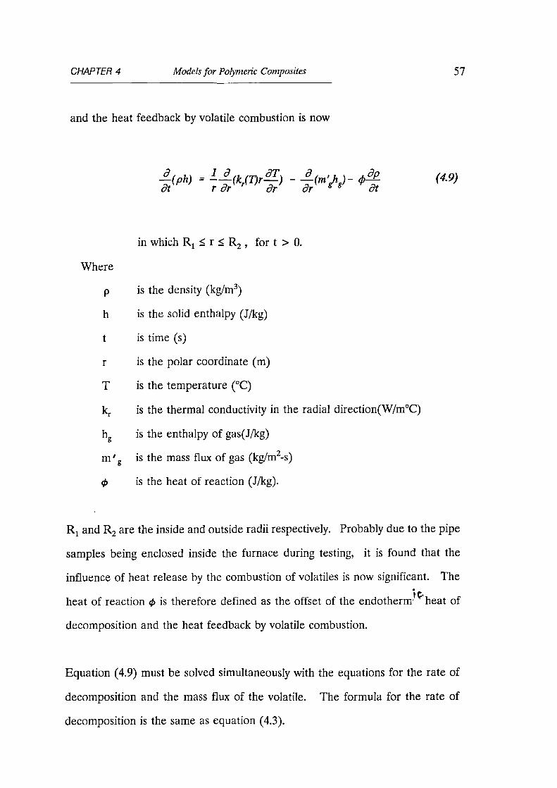
CHAPTER 4 Models for Polymeric Composites 57
and the heat feedback by volatile combustion is now
—0 (ph) = —1 —0 (Icr(T)r—dT) - —
8 (m'ghg)- (0
8p
Ot r Or Or 8r 8t
in which R1 � r � R2 , for t > 0.
Where
P is the density (kg/m3)
h is the solid enthalpy (J/kg)
t is time (s)
r is the polar coordinate (m)
T is the temperature (°C)
kris the thermal conductivity in the radial direction(W/m°C)
hgis the enthalpy of gas(J/kg)
m' g is the mass flux of gas (kg/m2-s)
cis is the heat of reaction (J/kg).
R1 and R2 are the inside and outside radii respectively. Probably due to the pipe
samples being enclosed inside the furnace during testing, it is found that the
influence of heat release by the combustion of volatiles is now significant. The
lc.heat of reaction 0 is therefore defined as the offset of the endotherm heat of
decomposition and the heat feedback by volatile combustion.
Equation (4.9) must be solved simultaneously with the equations for the rate of
decomposition and the mass flux of the volatile. The formula for the rate of
decomposition is the same as equation (4.3).
(4.9)

aneg _ _op
ar at(4.10)
CHAPTER 4 Models for Polymeric Composites 58
If the accumulation of gases and the effect of expansion on density change are
ignored, the conservation of mass can be written approximately as:
The mass flux, m ' g, at any spatial location and time can be calculated by
integration of equation (4.10).
Equation (4.9) is modified to its final form by expanding the first three terms,
substituting in the specific heat and the continuity equation and rearranging. This
results in
aT apC —61' = —
1 y.a—
g
0(k (7)r—) - in C — --il.(0÷12-Its,)
P at r ar r Or ' ar at(4.11)
where
Cp is the specific heat of the material (J/kg°C);
Cpg is the specific heat of gas (J/kg°C).
Equations (4.3),(4.10) and (4.11) form a set of non-linear partial differential
equations in polar coordinate which may be solved simultaneously for p, m , g and
T, respectively.
The boundary conditions on the exposed and unexposed sides of a pipe may be

CHAPTER 4 Models for Polymeric Composites 59
a prescribed temperature or radiative and convective boundary condition. As
previously, in order to exclude the uncertainties of the heat transmission rate from
the fire to the samples, the measured temperature was used at the exposed outer
surface. While for the unexposed inside, an adiabatic surface is assumed due to
the heat capacity of the inside air being negligible.
The equation (4.11) was solved by a simple and effective numerical scheme,
namely the 1-D explicit finite difference method. By using the energy balance
technique, the finite difference equation for an interior node can be obtained:
Ti#1 = 1m+ 2 At lk
pCp [(rm -Ori/4)6r1 +(rm +Or2/4)6r21 m'm4
(rmgr2+0.5)(Th;+1-T,D+km_i,m(rmgr1-0.5)(7,lh_1-T;)]
- (5p(O+h-hs)/pCp
(4.12)
Since the thermal expansion is required to be included into the model, the spatial
interval between the nodes will change according to the temperature, despite the
nodes being initially uniformly spaced. Six mesh nodes across the thickness of
pipe were used. It is assumed that the inside surface does not move during
expansion at high temperature. The second term on the right hand side of
equation (4.11) can be ignored under the powerful heat impingement on the pipe
experienced during a furnace fire test.
For node 1 on the inside surface,

CHAPTER 4 Models for Polymeric Composites 60
Tr.i _ Tit 4. 21c1.2(r 1 +0.5 Or)dt (7.'
4(0 -/-h -hg)
pCp(r1 -i-a25Or)(6r)2 2 1 PCp(4.13)
4.5 Model for the Intumescent coatings
As described above, the heat transfer analysis for the intumescent coating GRP
pipe under fire is a complex task due to the physical and chemical processes arewe e.
concurrent. Therefore, several idealizations .., made:
1). The intumescent material is assumed to be homogeneous and the
transmission of heat and mass is only in the radial direction of the
cross-section. Then, for a straight pipe, the problem is one
dimensional.
2). There is thermal equilibrium between the decomposition gases and
the solid material and there is no accumulation of these volatile
gases in the solid material.
3). The fissures that occur in the residual char are ignored in the
model. Only the average performance was taken into considered.
Based on these assumptions, a one-dimensional energy equation in a coated pipe
undergoing thermal decomposition is formulated which expresses a balance

CHAPTER 4 Models for Polymeric Composites 61
between the transient energy accumulation rate, with the sum of the rates of
conduction, pyrolysed convection, and the energy sink due to pyrolysis and the
heat released by volatile combustion
d OT a alt—a 1(mh) = --(ki —WM --ar—(ne,h
g ) -0 (4.14)
at r dr ar 6 at
in which R1 � r .s. R2 , for t > 0.
Where
m is the mass (kg)
h is the solid enthalpy (J/kg)
t is time (s)
r is the polar coordinate (m)
T is the temperature (°C)
kris the thermal conductivity in radial direction(W/m°C)
hgis the enthalpy of gas(J/kg)
m' g is the mass flux of gas (kg/m2-s)
4) is the heat of reaction (J/kg).
RI,R2 are the inside and outside radii respectively.
The mass of intumescent material is assumed to be composed of two parts
(4.15)
where ma is mass of active material and mc is the mass of residual char.

CHAPTER 4 Models for Polymeric Composites 62
The rate of decomposition of the active material is assumed to conform to a mean
reaction which is described by a single first-order Arrhenius function
an la _ A rn a eXP( -E A/RT)
at(4.16)
If the accumulation of gases is ignored, the conservation of mass is given by
= (Ina -a (nt)drdAOt at Or
(4.17)
Following the treatment of [4.11], the amount of expansion of the intumescent
coating is associated with the mass loss:
MO -111zlr = Aro n +(E -1)( )n1
mo-mc
(4.18)
where
mo is the original mass
mc is the char mass
is the current mass
E is the maximum expansion factor
is the exponent which describes the dependence of
expansion on the change in mass from mo.
Equation (4.14) is modified to its final form by expanding the terms, substituting
in the specific heat and the continuity equation, and rearranging. This results
in

CHAPTER 4 Models for Polymeric Composites 63
k aTmC —ar = —d (k —
aT)drtIA +
P at 8r r er r er(4.19)
L L OMffArAA 47i at-171 g Pg Or
where
C is the specific heat of material (J/kg°C);
CPg is the specific heat of gas (J/kg°C).
,<-The initial conditions for !at t = 0 are
T.Ti; ..m0 ; neg =0 • (4.20)
where Ti is initial temperature (°C);
Equations (4.16) to (4.19) form a set of non-linear partial differential equations
which may be solved simultaneously for m, m g and T respectively.
The boundary conditions on the exposed outer side of a pipe could be either a
prescribed temperature or a radiation and convection boundary condition. To
exclude the uncertainties of the heat transmission rate from the fire to the
samples under test, the measured temperature was used as the boundary
condition at exposed side. While for the unexposed inner surface, the adiabatic
condition is assumed because the ends of pipe were blocked and the specified
heat capacity of the inside air is negligible.

CHAPTER 4 Models for Polymeric Composites 64
The equation (4.19) was solved by a simple and effective numerical scheme,
namely the explicit finite difference method. By using the energy balance
technique, the finite difference equation for a typical interior node i in the
intumescent layer can be obtained:
= T f
ki#1 A0(ri/Ar1 +0.5)(7 —
• y2 - (o+h-hg)1 At
C ,d0r.(T. -T.pg s +IAt miCp
where a prime ' denotes the temperature at the next time step.
(4.21)

65
CHAPTER 5
Effects of Intrinsic Properties of Materials
5.1 Conventional Thermal Properties
To understand the thermal response of the components of construction to the
high temperatures experienced in a fire, it is important to have a knowledge of
the thermal properties of materials and their changes with temperature. The
difference in performance of insulation materials is mainly determined by their
capability to attain a high surface temperature without conducting significant heat
into the substrate. For simple systems it may be adequate to say that it is the
rate of deterioration of the material properties which determines the fire
resistance that the construction is capable of providing. It is well known that the
values of the thermal properties of the constituent materials play a crucial role in
the numerical modelling of heat transfer in a construction element. A knowledge
of the variations of thermal properties with temperature and other circumstances
is essential for the prediction of the rate of heat transfer into the construction.
The conventional thermal properties which will be considered in this section refer
to thermal conductivity, specific heat and emissivity. For most materials, these
properties are temperature-dependent. Among them the thermal conductivity
of the material has the most significant effect on heat conduction. It is found

CHAPTER 5 Intrinsic Properties of Materials 66
that even a relatively slight variation of the conductivity can cause a substantial
change in the predicted temperatures.
non-porousHeat transmission solely by conduction can take place only in _ , non-
transparent solids. In porous solids (most construction materials) the mechanism
of heat transmission is a combination of conduction, radiation and convection.
The thermal conductivity for such solids is, in a strict sense, merely a convenient
empirical factor that makes it possible to describe the heat transfer process with
the aid of the Fourier law. In this sense, the thermal conductivity is sometimes
called the effective (or apparent) thermal conductivity. The effective thermal
conductivity of most materials is a sensitive property relating to many factors.
These factors could be the temperature, the density, its gradient, the moisture
content, the degree of crystallinity, the average grain size, the mix proportions for
heterogeneous materials and the conductivities of its constituents, the porosity of
porous materials, and the type of fluid within its pores, etc. Therefore, in spite
of the many efforts that have been devoted to the determination of the effective
thermal conductivity of various materials under different circumstances for about
a century, total success has yet to be achieved[5.1-3]. It is easy to understand
why there are so many existing diverse and disparate data for some materials.
The surface emissivity of the material is also important as this will determine how
much heat will be gained from or lost to surrounding environment. It may also
vary with temperature and material physical state. Some materials can achieve
their effectiveness against certain types of fire by reflecting most of the fire
radiation. For instance, aluminium can survive well in non-engulfed conditions
and will stay cool for a longer time.
CHAPTER 5 Intrinsic Properties of Materials 67
In order to determine the values of thermal properties directly and explicitly,
various delicate experimental techniques are demanded. Since the direct
experimental measurement is complicated and time-consuming (it is even
necessary to make a distinction between conduction studies under steady state
conditions and those under transient conditions), the current situation is that there
is very little information available regarding the actual values to be used in
analysis. It is therefore necessary to regard the determination of the material
properties to be used in the analysis as an important part of this study.
An attractive possible solution to this problem is to extract material properties by
numerical techniques through systematically fitting the results given by
computation to the results of standard fire tests. The strategy which has been
adopted here is that, at first, approximate thermal properties are assumed. These
may be derived form the literature or from the values provided by the
manufacturer. These are then refined in order to take into account variations
with temperature, moisture, decomposition etc and to achieve a good correlation
between the numerical model and the test results. Once the thermal properties
under varying circumstances have been determined and agreed, the thermal
behaviour of this material under a variety of environments and configurations can
be modelled.
b,2 eioThis prediction-correction method has. 'proved to be a successful procedure and
is an important application of numerical techniques as practical results can be
obtained at low cost and with remarkable speed.
The first material which was tested was mineral wool sheet. Mineral wool is

CHAPTER 5
Intrinsic Properties of Materials 68
manufactured from long, non-combustible rock fibres bonded with a high
performance binder. Mineral wool slabs are easy to handle, cut and install and
incorporate high levels of thermal efficiency. The manufacturer, Pilkington[5.4]
only supplied the values of thermal conductivity up to 300°C for the sheet used,
namely type LR80 with a density of 80kg/m 3. The actual thermal conductivity
which was derived from the test results is shown in Table 5.1 for temperature up
to 1000°C. The values at other temperatures that are not listed in Table 5.1 are
assumed to vary linearly between the two nearest temperatures given in the table.
The specific heat is assumed to be 1000 J/kg°C.
The second material to be considered was Supalux, a Calcium-Silicate board
reinforced with selected fibres and fillers. It is the product of the Cape Boards
Limited. The manufacturer only supplies one value of thermal conductivity,
namely 0.17 W/m°C[5.5]. It was found that the numerical simulation can not
provide a satisfactory result when based on this constant conductivity. For this
material, the piece-wise linear variation with values of 0.16 W/m°C at 10°C, 0.18
W/m°C at 500°C and 0.3 W/m°C at 800°C was found to give the best fit. The
specific heat of calcium silicate board was chosen to be 1300 J/kg°C at 10°C and
800J/kg°C at 800°C. The moisture content in the tested sample was small and
negligible. The emissivity of the surface was chosen to be 0.6.
The thermal properties of hygroscopic materials and combustible materials will
display more complex patterns and they are discussed in the following sections.
CHAPTER 5 Intrinsic Properties of Materials 69
5.2 Effects of Moisture Content
Most practical construction materials contain some water and this has a significant
influence on the heat transfer mechanism and thermal properties. However, the
mechanism of the combination of heat and moisture transfer in elements of
construction is quite complicated. The process strongly depends on the
temperature, moisture distributions, chemical reactions, multiphase mass transfer,
permeability and nonlinear material properties[5.6]. Over past decades, several
studies have been carried out which try to take the influence of moisture into
account. Both sophisticated[5.9-10] and simple analytical models[5.11-12] have
been proposed. Sophisticated models consider the convective and diffusive heat
and mass transfer on the basis of an evaporation-condensation mechanism driven
by pore pressure and moisture concentration gradients. Despite the much
important work that has been done, there is still not a comprehensive and
satisfactory theory of the subject, and the existing theories (to the best of the
authors' knowledge) have not yet been able to find application in practice. The
simple engineering approaches, which mainly concentrate on heat transfer and
disregard mass flow and moisture pressure build-up, simulate the influence of
moisture by considering the energy demand of evaporation. They are easier to
apply and have the potential to yield an acceptable solution for the heat
conduction problem. However, if these models were not set up or used properly,
significant errors between prediction and experiment were often found at a
temperature range of about 90°C to 150°C[5.7,5.8] for hygroscopic components
exposed to fire.
CIDuring the heating of . hygroscopic material, a process of dissociation

CHAPTER 5 Intrinsic Properties of Materials 70
(dehydration), vaporization and migration of moisture takes place. For the
moisture to be evaporated, a certain amount of energy is needed, thus suppressing
the temperature increase. The moisture content in the materials could be in the
form of chemically or physically trapped water. The extra energy needed to
vaporize the moisture then comprises two parts: the heat absorbed in dehydration
process for chemical bonded water and the energy needed to drive off the water
(including physically absorbed free water) from the material. Under atmospheric
conditions, the heat of vaporization of water is 2.25x10 6, J per kg of water[5.13].
For most previous investigators this value was the only extra energy needed to get
rid of the water. Since they neglected the energy needed to dissociate the
chemically combined water and the additional energy consumed in the
evaporation-condensation cycle, noticeable errors were incurred.
LA)Ai t ,-,,
In - . il with the finite difference and finite element technique, an
improved engineering approach was developed in this thesis. As a example,
Redland gypsum plasterboard[5.14] was considered first, in which the gypsum
(calcium sulphate dihydrate, CaSO 4 . 2H20) is of about 95% purity. Gypsum-
board is one of the cheapest fire protection materials available, and normally has
a high moisture content (more than 15% crystalline water and a small amount of
absorbed free water). As gypsum is heated to temperatures in excess of about
95°C it begins to undergo a chemical reaction known as calcination, in which the
chemically bonded water dissociates from the crystal lattice. The chemical
equation for first the step is[5.15]
CaSO4 - 2H20 - CaSO4 . 1/21120 +3/21120 (5.1)

CHAPTER 5 Intrinsic Properties of Materials 71
Calcium sulphate hemihydrate (CaSO4 . 1/2H20) is commonly known as plaster of
Paris. The energy absorbed in the this process is approximately 100KJ per kg of
gypsum[5.15]. With further continued heating, the remaining water in the plaster
is released as the hemihydrate undergoes dehydration to form anhydrous calcium
sulphate, CaSO4. Then an extra 50KJ per kg is further consumed. By the time
the material reaches a temperature of around 155°C calcination in the board is
usually complete.
kikAccording toproposed approach, it is assumed that the moisture evaporation
takes place during a temperature range, for example 95°C to 155°C at each point
in the gypsum, and the latent heat energy of evaporation is then added into the
specific heat of material. The average: . additional specific heat is obtained by
DCp - 2
'25 x .1°6e A (J/kg°C)
AT
where:
DCp is the average _ additional specific heat
is the moisture content expressed as a fraction by weight
AT is the magnitude of the given temperature interval
A is a correction factor.
Then for example, assuming the gypsum contains 20% water by mass, the energy
needed to vaporize this water according the heat of vaporization (2.25MJ per kg
water) is 450KJ per kg of gypsum. The additional energy required in the
dissociation reaction (5.1) is 150KJ per kg of gypsum. According to this, A =
1.33 is established. The numerical analysis showed that although the result is
(5.2)

CHAPTER 5
Intrinsic Properties of Materials 72
better than that with A = 1.0, the demanded energy is still under-estimated.
Actually, it is found that the results with A = 1.8 give a satisfactory correlation to
the experimental results. This means that extra energy is required for the
moisture evaporation-condensation migration under high pressure.
In order to conform with the experimental measurement of the apparent specific
heat[5.15] and in order to keep the numerical stability, a triangular variation of
the additional specific heat is adopted as shown in Fig.5.1. Nevertheless, the total
energy which is needed to evaporate the moisture, in fact, is not altered.
Fig.5.1 The variation of ACp in a temperature interval 60°C
In equation (5.2), the value of the temperature interval AT should be selected
based on experiment. However, the most important parameter for the successful
modelling is the total amount of absorbed energy and the final temperature
development of modelling is not very sensitive to the value of AT.

CHAPTER 5 Intrinsic Properties of Materials 73
Following this treatment, the rate of increase of temperature will be suppressed
(but not halted as in traditional models) in the range of temperature AT, and a
gradual increase of temperature during vaporization can be simulated.
No value of specific heat is given by Redland for their plasterboard. However
reference[5.15] gave 950 J/kg°C for the specific heat of plasterboard with 3.4%
free water of the mass of the gypsum specimens and 14.6% water of
crystallization. Normally, the specific heat of a heterogeneous material can be
weighted by the fractional extent of each component
C = E n FC,, i=1 i C pi
where Fi is the weight fraction of each component and EFi = 1.
Then according to formula (5.3), with specific heat of water taken as 4200 J/kg°C,
the specific heat of dried plasterboard is 237 J/kg°C. This value is obviously too
low for dried plasterboard. It can be concluded that a modification of (5.3)
should be imposed for the chemical bonded water. Half of the weight fraction
of the chemically trapped water is tried. Then the specific heat of totally dried
plasterboard is set to be 629 J/kg°C.
Since the presence of moisture also has a significant effect on the thermal
conductivity, the determination of the thermal conductivity of moist materials
under fire is complicated. The thermal conductivity of building materials rises
considerably when the materials are even slightly damp. It is not only because
that some of the gaps in the solid matrix bridged by water, which is a better
(5.3)

CHAPTER 5 Intrinsic Properties of Materials 74
conductor of heat than air, but also because additional heat can be transferred by
the migration of moisture. The general expression for thermal conductivity and
moisture content can be
k(M) = k(0) T(vr)
(5.4)
where k(M) is the thermal conductivity at a moisture content M percentage by
volume and r(M) is the proportion factor.
The relationship between the proportion factor and the moisture content is not
a linear one, but an empirical formula can be derived to adjust the measured k-
value of masonry materials to an appropriate moisture content M based on a
relationship recommended by Jakob[5.16]:
r = 1.0819 +0.17675 xM -8.7812 x10 -3 xM 2 +1.7617 x10⁻⁵M3
(5.5)
To reduce the error of r, the value r = / when M = 0 is not used in curve
fitting.
The thermal conductivity, therefore, at an arbitrary moisture content can be
determined by a simple mathematic algorithm manipulating equations (5.4) and
(5.5) in the case where one reference thermal conductivity is known at a certain
moisture content.
Three types of Redland plasterboard were examined[5.14]. They are Wallboard
Type 1, Firecheck Type 5 and Firecheck Coreboard Types 4. Redland
CHAPTER 5 Intrinsic Properties of Materials 75
plasterboard consists of a gypsum plaster core bonded between two strong liner
pulp boards. The thermal conductivity of Wallboard provided by the
manufacturer[5.14] is 0.20 W/m°C. The Firecheck plasterboard consists of a
gypsum plaster core with glass fibres and fillers. The thermal conductivity of
Firecheck according to the manufacturer is 0.24 W/m°C. Redland Firecheck
coreboard consists of a gypsum plaster core with glass fibres and moisture
resistant liner boards. The value of the thermal conductivity is 0.22 W/m°C.
This has been confirmed by the measurements conducted recently by Dr.
s A ,rcA.Simson in _ university. The values of these thermal conductivities are close
to those quoted by another source[5.17] which gave the value of thermal
conductivity between 0.15 - 0.27 W/m°C.
Nevertheless, these are the values of conductivities at room temperature. In fact
the thermal conductivity will increase with increasing temperature at a certain
moisture content[5.2]. On the other hand, the total moisture content is gradually
reduced as heating proceeds during a fire. Therefore the final value of apparent
tke.conductivity should be the resultant of both effects. For r plasterboard, it is
found by numerical analysis that the effective thermal conductivity only displays
a slight increase with temperature when in the moist state.
The thermal conductivity of a material in a dried state at room temperature could
also be derived from (5.4) and (5.5). For dried materials, the fire resistance
capacity usually degrades at elevated temperature. Then the value of
conductivity will increase with increasing temperature. For the problem analyzed,
a linear variation of thermal conductivity with temperature is considered as a
reasonable assumption. Hence, for dried plasterboard, it is found that

0.4
0.3
obtained by this paper./
Given by ref.15.15 0.2 -
0.1 -
_
CHAPTER 5 Intrinsic Properties of Materials 76
k(T) = k(0) + 1.1 x10 - 4 xT (W/m °C) (5.6)
gave the best fit with the test data.
An interesting observation is that the values of thermal conductivity of gypsum
board extracted by above analysis and numerical procedure, which was mainly
done in 1993[5.18], is quite consistent with the results which were discovered later
in reference [5.15] (1994) by using a commercially available thermal conductivity
meter, as shown in Fig.5.2. The capability and potential of the computational
technique is astonishingly exhibited in this representative example.
Thermal Conductivity (W/m C)
100 200 300 400 500 600 700 800 900
Temperate (Deg C)
Fig.5.2 The Comparison of Thermal Conductivity of Gypsum Board
CHAPTER 5 Intrinsic Properties of Materials 77
The plasterboard is usually covered by paper so that surface emissivity selected
should be the value for liner boards manufactured from long fibre pulp. The
value 0.8 is chosen[3.1] for the unexposed face. On the exposed side, the value
of 0.4 is assumed due to the board burning away during fire exposure. The
density of plasterboard was measured before the test(see Table 5.2). The
numerical program calculates the new density automatically as water is driven off.
Based on the above-mentioned treatment and properties, a good correlation with
the experimental results was obtained (for details, see Chapter 6).
The second material which was tested is concrete. A two-dimension model based
on the finite element method for the concrete deck slabs will be described in
Chapter 8. For the present studies, only simple flat panels with low moisture are
considered. These were made from a mixture of ordinary Portland cement,
normal aggregate and febspeed by an undergraduate student. Before fire testing,
the concrete panels were dried in an oven to remove most of the moisture.
However there was still a small residual water content which was measured to be
0.9% by weight. Quite similar to the behaviour of gypsum, the hydrated cement
contains free calcium hydroxide which loses its water at high temperature, leaving
calcium oxide. Therefore extra heat for dewatering and dehydration is needed.
According to the guidelines given by the ECCS[2.5], the thermal conductivity of
concrete (with 0.9% moisture content) is chosen to be 1.5 W/m°C at room
temperature and approaches 1.02 W/m°C at high temperature. The values for
the completely dried concrete are 1.09 to 0.85 W/m°C. The specific heat is
between 900 - 1300 J/kg°C and surface emissivity is 0.8. An excellent agreement
between theory and test was again obtained (see Chapter 6).

CHAPTER 5 Intrinsic Properties of Materials 78
Another material which we tested with moisture content is Salford Voidfill. The
constituent materials are those known to have good fire resistance: namely perlite
and high alumina cement. Mixtures of 40% perlite filler, 60% cement and water
have been used to cast 50mm thickness samples which were fired up to 1125°C.
Because the thermal properties of this material are initially unknown, a
systematical calculation was conducted to determine these values. It was found
that the conductivity is around 0.07 W/mK with 10.6% water content at room
temperature and its maximum value is 0.24 W/mK at high temperature. While
the range of conductivity is 0.04 - 0.18 W/mK in a totally dried state. The specific
heat of dry material is 1000 J/kg°C approximately.
It should be noticed that the correction factor A may have a slight variation under
different circumstances. According to the previous explanation, the constituents
of the material and the configuration of the component may affect its magnitude.
Based on this modified treatment and chosen properties, reasonable agreements
with test results even at high levels of moisture content(up to 20% by weight)
have been obtained (see Chapter 6).
53 Kinetic Parameters for Pyrolysis
The thermal response of an organic material is significantly sensitive to the stage
of decomposition and the rate of density change. This is to be expected since the
rate of energy consumption and the thermal and transport properties of the

CHAPTER 5
Intrinsic Properties of Materials 79
material are functions of the constituents and the rate of decomposition. The
values of kinetic parameters A and EA in equation (4.3) will determine the
intensity and duration of decomposition corresponding to a given intensity of heat
flux. Since the in-situ measurement of parameters A and E A under the desired
thermal condition is intricate, the current practice is to use estimated values which
give good agreement between simulation and experiment. It is found that A
and EA depend on the rate of heating dT/dt. Therefore, for better modelling
without making the model unnecessarily complicated, two sets of values of A and
EA are assumed for inner hot and outer cold sections of panel respectively, as
shown in Table 5.3 and 5.4. The values of activation energy are generally
consistent with the results for plastic resin quoted by Samuel L. Madorsky in his
book[5.21].
Despite the fact that the parameters A and EA have their own meaning, altering
either A or EA can give a similar result for mass loss rate, as shown in Figs.5.3-5.
As an example, the initial values A and E A are set as A = 800/s and EA =58000
J/mol (Fig.5.3). Then either by changing the A to 400/s or E A to 62000 J/mol,
almost identical results are obtained (Figs.5.4 and 5.5).
In reference[4.5], Hender.lson et al employed a distinct approach in which they
separated the pyrolysis ratings into two separate regions according to the ratio of
m/mo where m is the remaining mass and mo is the initial mass.
The variation of thermal conductivity will also display a rather more complicated
pattern because it will be changed with temperature and the stage of
decomposition. It also depends on the type of resin used and the ratio of resin

CHAPTER 5 Intrinsic Properties of Materials 80
and glass for GRP material. One reference[5.19] gave the values of thermal
conductivity of GRP from 0.2 to 0.3 W/m°C. Another reference[5.20] gave the
values of conductivity from 0.25 W/m°C at 20°C to 0.35 W/m°C at 1200°C. The
general expression for thermal conductivity is assumed to be a linear function of
temperature here
k = ko + a T
(5.7)
for different stages of decomposition. For a tested GR polyester panel, from the
starting of the test to the point where the char was consumed, the value of k. is
0.26 W/m°C and a is —1.356x10⁴ W/m°C2. The negative value of a indicates
that the thermal conductivity deceases due to the low conductivity of the char.
As heating continues, the char will be oxidized and eroded away, leaving the glass-
fibre alone. During this phase, k0 will retain its value at the end of the last stage
and a = 2.0x10⁻³ W/m°C2. The conductivity will now increase as the
temperature increases due to the char being lost and the crumbling of the glass
mat.
For phenolic laminate, the thermal conductivity is fixed as 0.28 W/m°C until the
char is totally consumed. After that, the thermal conductivity follows equation
(5.7) with a = 1.8x10⁻³ W/m°C2.
The actual variation of thermal conductivity is unknown and might be more
complicated, but for simplicity, it is assumed to be a linear function of
temperature during each stage.
CHAPTER 5 Intrinsic Properties of Materials 81
One reference[5.19] gave the specific heat of GRP as 950 J/kg°C and the
emissivity as 0.9. The specific heat of WR polyester laminate is also assumed to
be a linear function of temperature here: C p = 1000 + 0.8xT (J/kg°C). The
heat of decomposition is -2.5x10⁶ J/kg and the emissivity of the panel is 0.8.
The specific heat of WR phenolic laminate is: C p = 1300 + 0.3xT (J/kg°C).
The heat of decomposition is -1.6x10⁶ J/kg and the emissivity of the laminate is
0.85. The thermal expansion coefficient is chosen as 4x10 -4 (1PC) for both of
them. These data have been estimated on the basis of information either found
in the literature or by experiment.
For Ameron glass-reinforced epoxy 2000M pipes, the kinetic parameters which
were used in the calculation were: A = 800 s -1 , EA = 56,000 J/mol for cellulosic
fire and A = 1200 s-1 , EA = 52,000 J/mol for hydrocarbon fire. The thermal
conductivity is set as 0.24 W/m°C, until the char is totally lost. Then the
conductivity will follow the equation
k = 0.24 +1.2 x10 -3 T W/m °C
(5.8)
The increase of conductivity in this stage is due to the char being lost and the
cracking of wound glass-fibre. The glass-fibre content in the pipe by volume is
about 41%. The variation of specific heat with temperature is
Cp = 1270 + 0.230 xT (.I/kg °C)
(5.9)
The heat of reaction Q is chosen as -3x10⁴ J/kg and the thermal expansion
CHAPTER 5 Intrinsic Properties of Materials 82
coefficient is 5x10 -4 (11°C).
The second type of GRP pipe which we tested were BP phenolic pipe. The
kinetic parameters which were used in the calculation were: A = 1500 s-1 and EA
= 50,000 J/mol. The conductivity is found to be 0.3 W/m°C until the char is
totally lost. Under hydrocarbon fire condition, the char will be oxidized and
consumed quickly, and leave wound glass-fibre alone. Then from that point, in
equation (5.7), the value of k 0 will be 0.3 W/m°C, and a will be 1.6x10 -3 W/m°C2.
The glass-fibre content in the pipe by volume is estimated to be 57%. The
specific heat of GR phenolic material is also assumed to be a linear function of
temperature:
(5.10)C,, 1115 + 0.484 xT (J/kg°C)
The heat of reaction Q is chosen as -5x10⁴ J/kg and the thermal expansion
coefficient is 4x10 4 (1/°C).
For intumescent materials, both the famous Pitt-Char and reinforced Pitt-Char
were tested. Pitt-Char is an epoxy based material and is sometimes reinforced
with glass fibre. From above analysis, it can be seen that the thermophysical and
kinetic properties of intumescent materials have a significant influence on the heat
transfer rate. Unfortunately, most of these data are not available. One possible
solution for this problem is to undertake the direct experiment measurement
individually for each parameter. However, from the work described in
reference[4.10], one conclusion is, although the authors tried to determine all

CHAPTER 5 Intrinsic Properties of Materials 83
thermophysical and kinetic properties of intumescent materials by experimental
measurement, the final results of temperature development given by the
theoretical analysis was still unsatisfactory. The problem might be caused by the
fact that these parameters are very sensitive to the heating rate, configuration and
ambient environment, and it is almost impossible to copy these conditions in
measurements recorded during real fire tests. Therefore, estimated values were
used and refined which can give good agreement between the experimental and
numerical results. The adopted thermophysical parameters which were used in
numerical calculation for Pitt-Char and reinforced Pitt-Char are listed in Tables
5.5 and 5.6.
The numerical simulations which were based on above quoted parameters all
present a satisfactory correlation with the experimental outcomes (see Chapter 6).
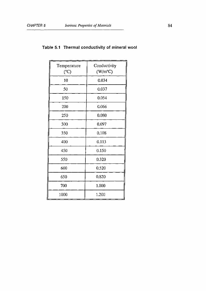
CHAPTER 5 Intrinsic Properties of Materials 84
Table 5.1 Thermal conductivity of mineral wool
Temperature
(°C)
Conductivity
(W/m°C)
10 0.034
50 0.037
150 0.054
200 0.066
250 0.080
300 0.097
350 0.108
400 0.113
450 0.150
550 0.320
600 0.520
650 0.820
700 1.000
1000 1.200

CHAPTER 5 Intrinsic Properties of Materials
85
Table 5.2 Data for plasterboard specimens
Sample Thickness
(mm)
Density
(kg/m3)
Moisture
Content (%)
(by weight)
Conductivity
(moist state)
(W/m°C)
la 12.5 836.4 17.5 0.20
2b 15.0 825.2 20.2 0.24
3c 25.0 856.4 19.4 0.22
4c 25.0 726.2 6.4 0.164t
4t Calculated by equ.(54) based on the reference conductivity 0.22W/m°C
Table 5.3 Kinetic parameters of GR Polyester panel
Cellulosic Fire Hydrocarbon Fire
A EA A EA
outer cold section 400 70000 600 68000
,, inner hot section 1200 54000 1200 54000

CHAPTER 5 Intrinsic Properties of Materials 86
Table 5.4 Kinetic parameters for WR Phenolic laminate ina hydrocarbon fire
A EA
outer cold section 600 60000
inner hot section 1200 58000
Table 5.5 Thermophysical Data of Pitt-Char (length=100cm)
mo mc kr(10°C) kr(1050°C) Cp (10°C) Cp(1050°C)
3.89 1.5 0.3 0.05 1380 1000
CPg
0 Em„ il A EA
2000 -6x10⁵ 3.33 0.2 2000 52000
Table 5.6 Thermophysical Data of Reinforced Pitt-Char (length=100cm)
mo mc kr(10°C) kr(1050°C) Cp (10°C) Cp(1050°C)
6.51 4.35 0.3 0.16 1300 900
CPg
CI5 Erna., n A EA
2000 -6x1a5 1.56 0.2 2000 52000
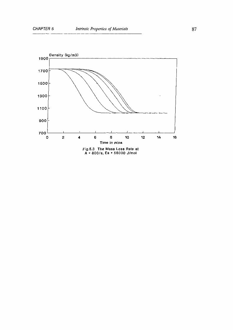
CHAPTER 5 Intrinsic Properties of Materials
Density (kg/m3)
87
1900
1700
1500
1300 -
1100 -
900 -
7000
_
-
I I I 1 1 1 1 1
2 4 6 8 10 12 14 16
Time in mins
Fig.5.3 The Mass Loss Rate atA - 800/5, Ea - 58000 J/mol

1
Fig.5.4 The Mass Loss Rate atA - 400/8, Ea • 58000 J/mol
1
CHAPTER 5 Intrinsic Properties of Materials 88
Density (kg/m3)1900
1700 -
1500 -
1300 -
1100 -
900
7000
Density (kg/m3)1900
10 12 14 16
I I I I
2 4 6 8
Time in mins
1700 -
1500 -
1300 -
1100 -
900 -
7000 2 4 6 8 10 12 14 16
Time in mins
Fig.5.5 The Mass Loss Rate atA - 800/s, Ea - 62000 J/mol

89
CHAPTER 6
Fire Test Results and The Verification of
Numerical Modelling
A description of the fire test facilities and the procedures used is given in a
supplement at the end of this thesis.
6.1 'Traditional' Fire Resistant Panels
To validate the accuracy of the numerical modelling and to determine the fire
performance of different materials, a number of standard fire resistance tests
were carried out for the materials which were described in Chapter 5. The
'simulated fire' tests were, and will continue to be, the principal means of
affirmation. Panels with different thicknesses and moisture contents have been
tested under the condition in which the temperature of a gas-fired furnace was
controlled to follow the BS476 cellulosic time-temperature curve[1.1]. The
computer program which controls the furnace uses a continuous PID three term
closed control loop system. The three terms are Proportional, Integral and
Derivative. By acting on an error signal E(t), which is the difference between the
instantaneously required temperature and the measured furnace temperature, the
PID method will achieve continuous control with a good accuracy[6.1].
The panels, most of them with an area of 300x300mm 2, were clamped in a
vertical position across an aperture in the door of the furnace with one side
exposed to the furnace environment, and open to the ambient air on the other

CHAPTER 6 Experimental Venfications 90
side. The ambient air temperature in the general vicinity of the test construction
fell into the interval of 5°C to 40°C specified by the standard[1.1]. The
temperatures of the exposed and unexposed sides of the panels and furnace were
recorded on hard disc every 20 seconds by the computer. The readings on the
centre of the exposed and unexposed sides were adopted to simulate the one-
dimensional heat transfer behaviour. According to BS476:part 20, there are two
fire resistance criteria for insulation failure based on the measured temperatures
on the unexposed face[1.1]. One criterion is that the mean unexposed face
temperature should not increase by more than 140°C above its initial value.
Another one is that the temperature recorded at any position on the unexposed
face should not exceed 180°C above the initial mean unexposed face temperature.
Because only the temperature at the centre of unexposed face, which is the
highest temperature on the surface, was measured, the second criterion was
adopted as an indication of material performance.
The thermal model was verified in two parts, separating the influence of two sets
of important parameters, namely the parameters describing conduction in the
panel and the parameters describing heat transfer from the furnace to the
specimen by convection and radiation. First, the heat conduction in the panel
was examined by applying the measured hot face temperatures as the hot side
boundary condition for the numerical simulation (first method specified in section
2.4). Secondly, the heat transfer rate from the furnace to the specimen was
calculated on the basis of the furnace temperature or the standard curve and the
assumed heat transfer parameters. In the numerical modelling, the cross-
section of each panel was subdivided to give six equally spaced nodal points.
Some typical results using the thermal properties quoted in Chapter 5 are
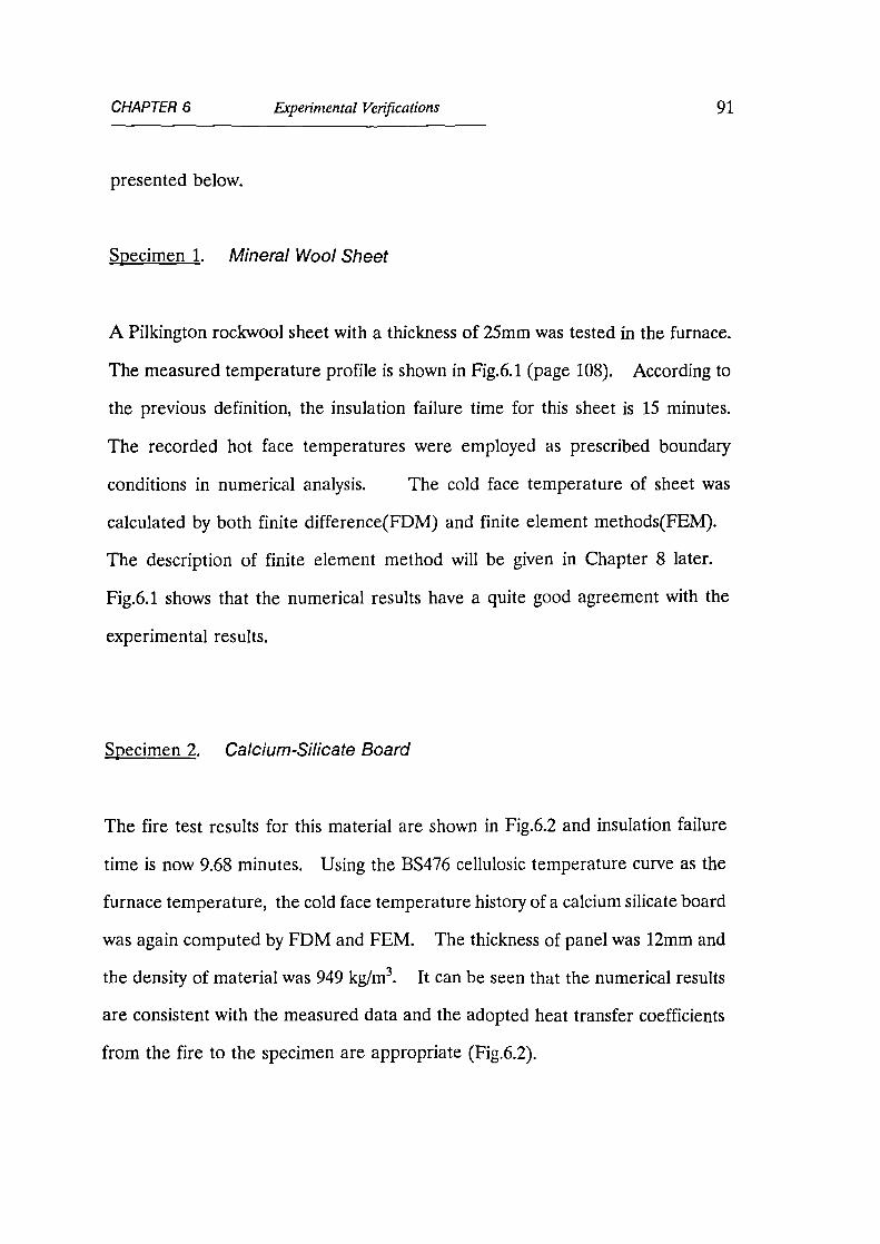
CHAPTER 6 Experimental Verifications 91
presented below.
Specimen 1. Mineral Wool Sheet
A Pilkington rockwool sheet with a thickness of 25mm was tested in the furnace.
The measured temperature profile is shown in Fig.6.1 (page 108). According to
the previous definition, the insulation failure time for this sheet is 15 minutes.
The recorded hot face temperatures were employed as prescribed boundary
conditions in numerical analysis. The cold face temperature of sheet was
calculated by both finite difference(FDM) and finite element methods(FEM).
The description of finite element method will be given in Chapter 8 later.
Fig.6.1 shows that the numerical results have a quite good agreement with the
experimental results.
Specimen 2. Calcium-Silicate Board
The fire test results for this material are shown in Fig.6.2 and insulation failure
time is now 9.68 minutes. Using the BS476 cellulosic temperature curve as the
furnace temperature, the cold face temperature history of a calcium silicate board
was again computed by FDM and FEM. The thickness of panel was 12mm and
the density of material was 949 kg/m 3. It can be seen that the numerical results
are consistent with the measured data and the adopted heat transfer coefficients
from the fire to the specimen are appropriate (Fig.6.2).

CHAPTER 6
Experimental Verifications 92
Specimens 3-6. Four Plasterboards
The proposed moisture model was verified by testing four plasterboards with
different thickness and moisture contents. The data for these panels are
summarised in Table 5.2 and their insulation failure times are shown in Table 6.1.
Table 6.1 Insulation Failure Time for Plasterboard Specimens
Sample Thickness
(mm)
Moisture Content
(% by weight)
Insulation Time (
(mins)
la 12.5 17.5 25
2b 15.0 20.2 32.4
3c 25.0 19.4 76
4c 25.0 6.4 45
ej t C IJ 4 ,By comparison with the -; _ . 5: the insulation time is extended
considerably due to the moisture effect. The 'dwell' of temperature rising on the
unexposed face of the samples can be easily seen from the water loss plateau in
Figs.6.3 to 6.6.
In the finite difference calculations, the boundary condition on the exposed side
of samples was prescribed by the measured temperature. The computed

CHAPTER 6 Experimental Verifications 93
temperature history on the unexposed side was then compared to the measured
results (Figs.6.3 to 6.6). It can be concluded that the simulation of the moisture
effect is quite successful in these cases. This demonstrates that the influence of
different percentages of moisture on the fire resistance can be predicted
accurately.
At the same times the selection of the associated thermophysical properties is also
validated by these specimens. The reason for the small deviation between the
calculated and measured data over 230°C on unexposed face is probably because
some small cracks begin to appear on the exposed side of plasterboard at that
temperature. Then the prerequisite of a continuum for the validity of equation
(2.1) no longer exists.
The modelling of the heat transfer from the fire compartment to the specimen
was also verified by plasterboard 3c. The selections of heat transfer parameters
to simulate the heat transmission from furnace to specimen are specified in
section 2.4. The computational temperature history of the exposed and
unexposed faces are compared with experimental results in Fig.6.7. A good
agreement is again noted.
Specimen 7. Plasterboard and Calcium-Silicate Sandwich Panel
The verification of the modelling for a multi-layer panel was carried out for this
case. A Wallboard plasterboard, thickness 12.5mm with 6.4% moisture content,
was combined with a calcium-silicate board, thickness 6mm in the dry state. The

CHAPTER 6 Experimental Verifications 94
insulation failure time is now 26 minutes. Identical thermal properties-
temperature relationships as used in previous calculations were also applied in this
case. The actual furnace temperature history was used as the exposed side
boundary condition and the heat transfer parameters were the same as those in
previous examples. Fig.6.8 shows that the numerical prediction gives a
reasonable agreement with the measured result. The discrepancy might be
caused by the assumption of perfect contact at the interface between two material
layers.
Specimens 8-10. Three Concrete Panels
Three normal concrete panels, as described in the last chapter, were also tested.
They have three different thicknesses namely 53mm, 77mm and 102mm
respectively. The moisture content of the concrete was 0.9% by weight after oven
drying. The corresponding insulation times were extrapolated as 42, 77 and 120
minutes. The measured temperature on the exposed side was also applied as
the boundary condition in the numerical analysis. Excellent agreement was
obtained when the numerical predictions were compared with the test data, as
illustrated in Figs.6.9 to 6.11.
Specimen 11. Salford Voidfill Panel with thin steel sheets
In this sample, the combination of hygroscopic core material and impervious skins
is investigated. The core material was Salford Voidfill No. 7D. Its density was

CHAPTER 6 Experimental Verifications 95
325kg/m3 and its moisture content was 7.02%. Two thin (0.7mm) steel sheets
were used as the faces of the sandwich panel during fire testing. The insulation
time was extrapolated as 230 minutes. An excellent fire resistance time was
therefore obtained.
The numerical calculations showed that the heat resistance of the thin metal
sheets could be neglected. Nevertheless, the emissivity of these steel sheets
should be adopted as actual surface emissivity of sandwich panel on the
unexposed side. The measured furnace temperature was used as boundary
condition on exposed side. The calculated cold face temperature development
shows a reasonable agreement with experimental result (Fig.6.12).
An imperfection in this testing arrangement was that the periphery of the panel
was not insulated. The moisture might escape more easily from the edges of this
relatively small sample compared with large scale samples. Therefore, the
magnitude of the thermal conductivity which was derived from this test might
over-estimate the value that would be appropriate for an actual full scale panel.
6.2 VVR Glass-fibre Reinforced Polyester Laminates
The polyester and woven roving glass-fibre laminate was made with thermocouples
(K type) embedded inside the central region in order to measure the temperature
profile history across the cross-section of the laminate, as shown schematically in

CHAPTER 6 Experimental Verifications 96
Fig.4.1. The resin which was used for the baseline testing was Crystic e 489 PA
unsaturated polyester resin which based on isophthalic acid and supplied by Scott
Bader Company Ltd. The reinforcement was Owens Corning E-glass-fibre
woven roving at 600 gsm for the laminate. Since full-scale testing is very
expensive, model-scale testing has again been developed for material
characterisation tests of the type required for this investigation. The polyester
laminates were made using a hand lay-up technique and cured at room
temperature.
Series of both simulated cellulosic and hydrocarbon fire tests have been canied
out. Since, in the small furnace that was used for these tests, it is impossible to
achieve the initial rapid rate of temperature increase needed for hydrocarbon fire
simulation, the furnace was first pre-heated to 900°C. During this heating period,
the blanking panel was in place with a dummy piece of material covering the
window opening. Immediately after switching off the furnace, the dummy piece
of panel was removed and replaced by the test piece and the furnace was
switched on again. A point on the hydrocarbon time-temperature curve was then
attained within a few seconds.
The size of each panel was 380x380mm 2 with an area 250x250mm2 exposed to the
furnace. In the cellulosic fire tests, the average thickness of the panels was
5.9mm and the polyester resin content was 31% by weight. In the hydrocarbon
fire tests, the average thickness of the panels was 6mm and the resin content was
33% by weight. The density of the resin was 1130 kg m3 and that of the fibre
glass was 2560kg/m3. The catalyst for the resin was 1.5% by weight of Catalyst M.
The number of glass plies in all of the panels was 13. Due to the scatter of

CHAPTER 6 Experimental Verifications 97
experimental data on a sample-to-sample basis, for both series of fire tests,
several samples with the same configuration were tested and the average test
results were compared with the analytical results. Normally the measured
deviation among the samples was within 10% if there was no local delamination.
The general trend of the temperature history, most noticeable on the unexposed
side, was that, at the beginning of test, the temperature increased at a moderate
rate. When the material started to decompose, the rate of temperature rise was
slowed down due to the energy absorbed in pyrolysis. However, after the cracks
appeared in the char and char was consumed, the temperature increased rapidly
again (see Figs.6.13 and 6.14)
The cellulosic fire test lasted for about 40 minutes whereas, in a hydrocarbon fire,
the 6mm thick panel can only survive for about 15 minutes. The lime lo
insulation failure in a cellulosic fire was 7.8 minutes, while, in a hydrocarbon fire
it was 5.3 minutes. This shows that, if thin GRP panels are used alone, they are
insufficient to supply a satisfactory performance in terms of heat insulation under
fire condition. Therefore, a good practice is to combine them with low density
fire resistant core material in a sandwich construction. For this reason the single
panel tests were sustained well beyond insulation failure until the cold face
temperature reached about 400°C.
In the finite difference analysis of these tests, eight mesh nodes across the
thickness of panel were used. The measured temperature-time history on the
exposed was used as the hot face boundary condition.
Several points of interest were discovered in the course of the numerical

CHAPTER 6 Experimental Verifications 98
investigation. The first one is that the second term of the right side of equation
(4.6) can be ignored. The physical meaning of this term depends on the
direction of the flowing volatile. The main part of the volatile flows outward and
has a cooling effect on the exposed side of panel while the inward flowing
component enhances the heat flow to the inside. It was found that the net effect
can be neglected by comparison with the powerful incident heat flux that was used
in the furnace tests. It seems that the endothermic pyrolysis and poor
conductivity of the char play a much more important role than internal
convection. The second point is that the accuracy of results will be improved if
the influence of thermal expansion is included into the model. The expansion
will increase the thickness of panel and this has an obviously beneficial effect on
the heat insulation of the panel. The thermal expansion coefficient was chosen
as 5 x 10⁴ (vac) for the glass-reinforced polyester panels considered here. This
figure is obviously much larger then the value within the normal temperature
range. When this effect is included in the finite difference analysis, the spatial
interval Ax in the panel changes with temperature.
The reduction of resin density given by equation (4.3) can be seen from Figs.6.15
and 6.16 for both fire tests. Evidently that there are different mass loss rates for
the inner hot part and the outer cold part of the panel. This coincides with the
experimental observation of the two-peak shape of mass loss rate[6.2], and the
final amount of remaining mass in the tested samples generally agrees with the
numerical predictions.
The comparisons of the predicted and measured temperature profile histories for
both series of fire tests are shown in Figs.6.13 and 6.14. The dashed lines

CHAPTER 6 Experimental Verifications 99
represent the transient temperature given by the numerical analysis for the same
spatial location as the thermocouples. The agreement between them is
reasonably good.
In order to gain further confidence in the numerical modelling, an additional
verification test was designed using same basic materials but with a different resin
content and thickness. For this test the resin content was increased to 42% by
weight and the number of glass plies was 16. The final thickness of panel was
measured as 8.8mm. A hydrocarbon fire test was carried out and the time to
insulation failure was found to have increased to 7 minutes. As shown in
Fig.6.17, good correlation between theory and experiment was again obtained
by using the same thermal properties as previously.
Bearing in mind the rather steep thermal gradient inside the relatively thin
laminate tested, the calculated results gave a quite good correlation with
experimental measurements. It appears that the fire resistance of a GR
polyester laminate in a standard fire test can be predicted well by the proposed
computational treatment.
There are, nevertheless, some discrepancies between the calculated and
measured results and these might have been caused by following factors. First,
the numerical model does not account for all of the physical processes which
occur within the material. For example, both the heat exchange between the
volatile and solid material and the char shrinkage are partly neglected. .:;
Some processes, for instance moisture evaporation, were included in an implicit
way (the value of decomposition heat contains some energy needed for moisture
CHAPTER 6 Experinzental Verifications 100
evaporation). Secondly, there are some stochastic variations that effect the heat
transfer and which are difficult to control such as the delamination and cracking
in the material and the positions of the thermocouples relative to these effects.
Delamination is also an important feature associated with the fire resistance of
GRP laminates. However, for polyester laminate, it may be not so crucial as it
is for phenolic laminate with a high moisture content. But it should,
nevertheless, be mentioned as one possible reason for the discrepancies in
Figs.6.14 and 6.17. Thirdly, most input data of the thermal properties were
deduced on an empirical basis. It is well known that the value of the thermal
properties plays a crucial role in the numerical simulation of heat transfer and,
unfortunately, there are considerable practical difficulties in the explicit
determination of material parameters at elevated temperature. Besides, some
parts of the limited published data can not be used directly due to differences in
the sample's preparation, test assembly and heat loading level. Hopefully, the
need for such data will encourage more work to be carried out in this area. As
more accurate property values become available, ever better results may be given
by the proposed models.
An additional sandwich panel was tested with aim of achieving H120 fire
resistance (H120 means the fire resistance time is 120 minutes under hydrocarbon
fire test condition). It comprised two polyester laminate skins and a new
Vermiculux core. This new Vermiculux is an 'improved' version of the calcium
silicate board product by Cape Boards Ltd. Vermiculux readily absorbs water
and this can significantly extend the measured fire resistance. In order to limit
its influence, the 60mm thick Vermiculux panel was dried to constant weight
(504Kg/m3) at 110°C before the fire test. Nevertheless, it was found that 11.3%

CHAPTER 6 Experimental Verifications 101
of chemical bonded water was still held in the material. The polyester laminates
consisted of 12 layers of glass with 67% glass content by weight. The thickness
of the hot face skin was 6.4mm and the cold face skin was 6.2mm.
The fire test was conducted by another Ph.D student, David Dewhurst. The test
result gave a fire resistance time of about 180 minutes which is comfortably in
excess of the H120 target. The computational simulation was carried out by this
author. The theoretical treatment included the model for polyester laminate,
multi-layer configuration and moisture content. Excellent correlation between
the theory and experiment was again obtained (Fig.6.18).
63 'VVR Glass-fibre Reinforced Phenolic Laminates
Two phenolic laminate specimens designated I and II, with thicknesses of 12.6mm
and 11.7mm respectively, were tested under the hydrocarbon fire regime. The
specimens were laid up by hand and subjected to 5 hours post cure at 80°C. In
the numerical model, nine mesh nodes across the thickness of each laminate were
used. It is assumed that, at 200°C, each node will split into two separated
points in order to simulate delamination. Each time-temperature curve (except
that at the outside surface) will then split into two as well, as shown in Fig.6.19.
Due to the random position of the thermocouples relative to the position of the
interstices in the thickness as well as spatially, the analytical result is considered
to be acceptable if the measured temperature falls within the interval between the
two disjointed curves.

CHAPTER 6 Experimental Verifications 102
The measured and calculated transient temperature distributions in laminate I are
shown in Fig.4.3 and Fig.6.19, respectively. The comparisons of them are shown
in Figs.6.20 and 6.21. The broken curves in the figures represent the transient
temperatures measured by the thermocouples and the solid curves are the
temperatures given by numerical simulation. It can be seen that the insulation
time was increased to 30 minutes due to the delamination and the computational
results gave a reasonable agreement with the test results.
The reduction of resin density given by equation (4.3) is shown in Fig.6.22 for
different locations within the laminate. Due to the limitation of the test facility
used, it was not possible to monitor the instantaneous amount of mass in the
laminate. Nevertheless, the final amount of remaining mass of the specimen
was measured, and it generally agreed with the numerical result.
In order to obtain further confidence in the numerical modelling, an additional
validation was carried out for laminate II with a thickness of 11.7mm.12
C Li t --p • c. A ye,,,s
Unfortunately, only the : _. -,r .., .. _ . at locations 1, 5 and 6(Fig.4.2)A
gave
temperature readings. This time the insulation time was found to be 28 minutes
due to the thickness being slightly reduced. Fig.6.23 shows a good agreement
between the numerical and measured results by using the same above quoted
thermal properties that were used for laminate I.
These comparisons proved that delamination is an important phenomenon which
is related to the fire resistance of phenolic laminate with a high moisture content
and which must be considered in the analysis model if a reasonable result is to be
obtained. A valid explanation has also been given for the somewhat bewildering
CHAPTER 6 Experiniental Verifications 103
outcome of the temperature measurements obtained when testing the phenolic-
woven roving glass laminate. It is evident that the fire resistance of GR phenolic
laminate in a standard hydrocarbon fire test can be predicted by the proposed
analytical treatment. The causes of the discrepancies are quite similar with
those in polyester laminate and will not be repeated.
6.4 Glass-Reinforced Plastic Pipes
For pipe problems, the one-dimensional model in polar coordinate has been
verified by the fire test results for Ameron glass-reinforced epoxy pipes and BP
phenolic pipes with different thicknesses. These pipes with a length of 0.5-0.8m
and with the two ends blocked by ceramic fibre were placed inside the large
furnace, which can simulate the hydrocarbon fire without preheating. For
hydrocarbon fire testing, the hydrocarbon time-temperature curve (Eq.2.20) was
followed for an initial five minutes, then the gas supply was cut off. This is to
simulate the start of a fire and the deluge response of the firewater system.
The outer and inner surface temperatures of the pipes were measured during the
test. The temperature inside the pipe is probably the best way to monitor pipe
performance under fire. The two dry Ameron pipes which were tested were a 3"
2000M pipe with an average thickness 5.7mm and a 4" 2000M pipe with an
average thickness of 5.4mm. The corresponding times for the inner temperature
to reach 200°C were 3.2 minutes for the 3" pipe in a cellulosic fire test and 1.7
minutes for the 4" pipe in a hydrocarbon fire test respectively (Figs.6.24 and 6.25).

CHAPTER 6 Experimental Verifications 104
The thermal properties which were used in calculation were specified in section
5.3. The measured temperatures on the outer surface was applied as a known
boundary condition. The comparisons of calculated and measured temperatures
on the inner surface for two pipes are shown in Figs.6.24 and 6.25. A good
correlation between both results is obtained.
Furthermore, three unprotected BP pipes were tested under hydrocarbon fire with
average thicknesses of 5.6mm, 7.7mm and 9.5mm respectively. The inside
diameter approximately was 75.8mm and density of the GRP was 1900kg/m3.
The corresponding times for the inside temperature to reach 200°C were 1.86,
2.75 and 3.5 minutes respectively. The thermal properties which were used in the
computation were also specified in section 5.3. The measured temperature
history on the outer surface was adopted as an essential boundary condition.
The comparisons of calculated and measured temperatures on the inner surface
for three different pipes are shown in Figs.6.26 to 6.28. The dashed lines
represent the transient temperature given by the numerical analysis. A good
agreement between calculated and measured results is again obtained.
Although, in order to keep the solution stable and to give good accuracy, the
time step At is chosen as 0.1 sec, the whole running time is less than 1 minute on
a PC486.
There are some deviations between the calculated and measured temperatures,
especially during the cooling stage. These might be caused by the following
factors. First, the numerical model does not precisely and explicitly account for
all of the physical processes which occur within the material, such as the
CHAPTER 6 Experimental Verifications 105
combustion of the volatiles and micro-cracks. Secondly, most of the input data
of thermal properties of material are given on an empirical basis and did not fully
account for the difference between the heating up and cooling down stages.
However, the results demonstrated that an appropriate set of data can produce
a consistent result for GRP pipes with different thicknesses.
After an initial five minutes fire impingement, either natural or forced cooling by
air was then commenced. It was noted that the pipe continued to smoulder or
burn during cooling and that this resulted in continuing damage to the pipe.
When the pipe had cooled sufficiently to be handled, its ability to hold water was
investigated. All the above type pipes failed to hold water under pressure after
fire testing. This revealed that the operable survival of unprotected thin GRP
pipes under the furnace hydrocarbon fire condition for more than 5 minutes is
unlikely. Therefore, an additional protection is needed and this can be achieved
by one of following methods: a coating of fire-retardant intumescent material,
mineral or ceramic wool wrapping, or by filling the pipe with stagnant or flowing
water. These methods have proved that they can considerably reduce the damage
to GRP pipes under fire as shown in next section typically for the intumescent
coatings.
6.5 GRP Pipes with Intumescent Coatings
Two Ameron 4" epoxy pipes with the intumescent coating Pitt-Char and
reinforced Pitt-Char were tested under a hydrocarbon fire. The Pitt-Char is also

CHAPTER 6 Experimental Verifications 106
an epoxy based material which is sometimes reinforced with glass fibre. The
average thickness of un-reinforced coating was 7.5mm and reinforced coating was
11.5mm. These straight pipes with a length of 0.7m and the two ends blocked by
ceramic fibre, were placed inside the gas-fire furnace which followed the
hydrocarbon temperature-time regime(Eq.(2.20).
The outer and inner surface temperatures of the pipes were measured during the
tests(Fig6.29 and 6.30). It can be seen that the temperature increase in the inner
surface of GRP pipes was significantly delayed in comparison with the fire test
result on the unprotected GRP pipe (Fig.6.25).
Although the reinforced coating is thicker than the un-reinforced coating, both of
them gave the similar results. This is because, although the reinforcement
enhanced the integrity and adhesion of the intumescent char, it also impeded the
swelling of intumescence.
The adopted thermophysical and kinetic data for intumescent coatings were listed
in section 5.3. The exponent n = 0.2 (see Eq.(4.18)) indicates that the expansion
occurred early in the outgassing stage which is consistent with the experimental
observations. The comparison between the measured and calculated temperature
profiles on the inner surface of pipe shows that a good agreement is obtained
(Figs. 6.29 and 6.30).
A relatively simple approach was developed to simulate the temperature history
of GRP pipes with intumescent coatings under the standard hydrocarbon fire
condition. The famous intumescent material Pitt-Char was chosen which normally
CHAPTER 6 Experimental Verifications 107
expanded 2-4 times the original thickness. The favourable correlation was
obtained between the experimental and theoretical results. For different
intumescent systems, it is anticipated that only the thermophysical parameters
required adjusting in the modelling.
6.5 Conclusions
All above-mentioned numerical calculations were completed in a few minutes by
a PC 486. The computational time is short and the cost is low. The
convergence of the numerical results was proved to be satisfactory for mesh
refinement and shorter time-steps. It can be concluded that the numerical
results based on the proposed thermal models provided a favourable simulation
of the fire resistance of panels and pipes and the cost for the numerical prediction
is insignificant.

800
Measured Hot Face Temp.\600 -
400 -FEM
200
BS476 Curve\-
Calculated (FD and FE)\\Measured
Neold Face Tema.
111 ,
1000
800
600
400
200
CHAPTER 6 Experimental Verifications 108
Temperature (DEG C)
0 5 10 15 20
25
30
36Time in minute
Fig.6.1 Fire Test of Mineral Wool SheetThe thickness of sheet is 25mm
Temperature (DEG C)
5 10 15 20
25
30 35Time in mins
Fig.6.2 Calcium-Silicate Board (12mm)BS476 Fire Boundary Condition

25 30
CHAPTER 6 Experimental Verifications 109
Temperature (C)1000
800
600
400
200
00
5
10 15
20Time in mins
Fig.6.3 Fire Test of Plasterboard lathickness 12.5mm, moisture content 17.5%
Computational and Experimental Results
Temperature (C)1000
800
600
400
200
00 10 20
30
Time in mins
Fig.6.4 Fire Test of Plasterboard 2bthickness 15mm, moisture content 20.2%Computational and Experimental Results
40
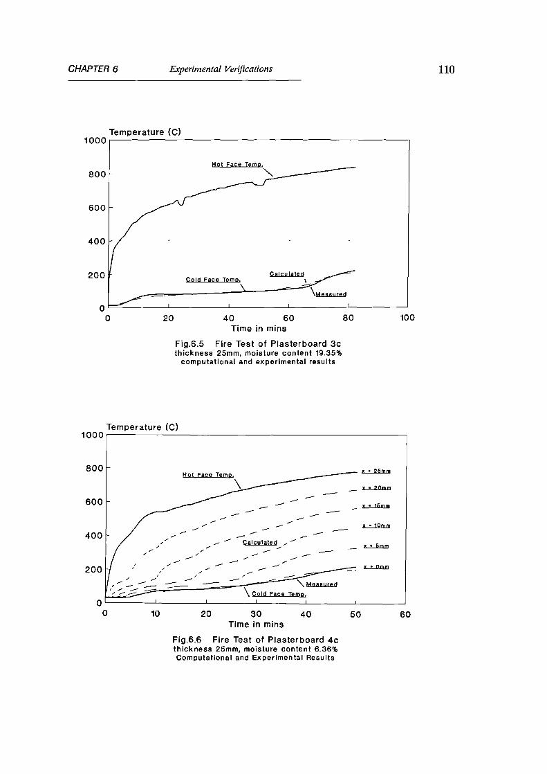
Hot Face Temo
Cold Face Temo Calculated
\Measured
1000
800
600
400
200
Temperature (C)1000
800 x • 26mmHot Face Tem),
is • 20mm
.....-....
600 .......,.......-.......
Wr2.0110.......,
.../..../....
............---......
../ - ...., • 10mm
400 ..-.----- ..-------- ...--
77
777
----
..-77
CalculatedCalculated 7...-..--
..--7....—
-- ,...-
...-
----
...-
200 //
-/
-// .../ ...--- .-...---- _v..-
- ..----• ...--- \ M e a s u red-- .---- -- \ Cold Face Temo,
CHAPTER 6 Experimental Verifications 110
Temperature (C)
20 40 60
80
100Time in mins
Fig.6.5 Fire Test of Plasterboard 3cthickness 25mm, moisture content 19.35%
computational and experimental results
10 20 30 40 50 60Time in mins
Fig.6.6 Fire Test of Plasterboard 4cthickness 25mm, moisture content 6.36%Computational and Experimental Results

Furnace Te/Measured---
-\Calculated
Hot Face Temo,
Calculated___,....„-----,.----- \Measured
1---------
- 83476 Curve\
^
,
Cold Face Temo,
0
20 40 60
80
100Time in mins
1200
1000
800
600
400
200
0
1200
1000
800
600
400
200
035 40
CHAPTER 6 Experimental Verifications 111
Temperature (C)
Fig.6.7 Fire Test of Plasterboard 3fire boundary modelling
Temperature (C)
o 5 10 15 20 25
30Time in mins
Fig.6.8 Fire Test of Multi-layer PanelPlasterboard and Calsium-Silicate Board

Cold Face Temp.
Measured
1 1
CHAPTER 6 Erperinzental Verifications 112
Temperature (C)800
Measured Hot Face Temp.600 - \
,/----------------
_400
200
Calculated%
__—
0
10
20 30
40
50Time in mins
Fig.6.9 Fire Test of Concrete Pane' 1Thickness of panel is 53mm
Temperature (C)
0
20
40
60
80Time in mins
Fig.6.10 Fire Test of Concrete Panel 2Thickness of panel is 77mm

,..._.__,---,---•--"---"'---'---'-"
\Furnace Tema.-
-
_Cold Face Temp.
Calculated
CHAPTER 6 Experimental Verifications 113
1000
800
600
400
200
0
Temperature (C)
1200
1000
800
600
400
200
0
20 40 60
80
100
120Time in mins
Fig.6.11 Fire Test of Concrete Panel 3Thickness of panel is 102mm
Temperature (C)
50 100 150 200 250Time in mins
Fig.6.12 Salford Voidfill Panel No.7DThickness of panel is 50mm
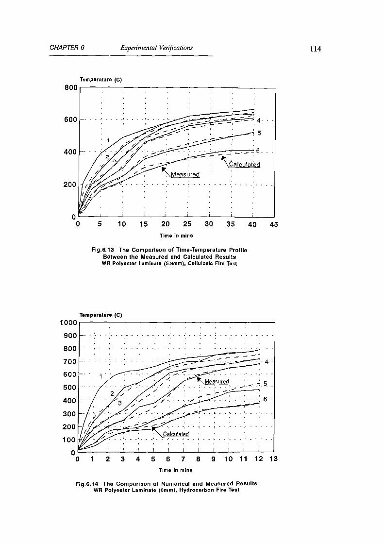
Temperature (c)
1000
900
800
700
600
500
400
300
200
100
o01I I I I 1 I 1
2 3 4 5 6 7
Time in mins
8 9 10 11 12 13
'
_
CHAPTER 6 Experimental Verifications
Temperature (C)
5 10 15 20 25 30 35 40 45
Time in mine
Fig.6.13 The Comparison of Time-Temperature ProfileBetween the Measured and Calculated Results
WR Polyester Laminate (5.9mm), Cellulosic Fire Test
114
Fig.6.14 The Comparison of Numerical and Measured ResultsWR Polyester Laminate (6mm), Hydrocarbon Fire Test

2000
1800
1600
1400
1200
1000o
CHAPTER 6 Experimental Verifications 115
Density (Kg/m3)
1 _1
5 10 15 20 25 30 35 40 45
Time in mins
Fig.6.15 The Mass Loss Rate at DifferentLocations of WR Polyester Laminate
Numerical Simulation for Cellulosic Fire
Density (Kg/m3)2000
1800
1600
1400
1200
1000I I I I I I I I _1
0 2 4 6 8
10
12
14
16
Time in mins
Fig.6.16 The Mass Loss Rate at DifferentLocations of WR Polyester Laminate
Numerical Simulation, Hydrocarbon Fire

Measured Hot Face Temo,
.6-.....---.-..... '-' ......
.. 4, 4 .......-...,-
/ ......4
4 / /..,
..,'/ ../
/ a a .....-/ ,--
/ 4----- -C alculated --
--4 ----
...---- ----4--- A— __---
/ /
/ A/ et 4 ------ •------4 _---- "7-4/
/ / --4--
/ / ,/ ...--
,,6 ,-,.•..-.. ,- ...--.' 4 ---M. ... ..,,s, easured
...- ..- ..- 4....4,
---' "-- -.-- 0. '''. 4
/ „......--- ,.......------- ass -- -a"
a
1000
900
800
700
600
500
400
300
200
100
20155 10
Time in mins
Fig.6.17 Hydrocarbon Fire Test ofWR Polyester Laminate (8.8mm, 42% resin)
Furnace Temp
Measured Results\
1200
1000 -
800
600 -
400 -
200 _ Cold Face Temp,
\Numerical Results
20
40 60
80 100 120 140 160 180Time in mins
CHAPTER 6 Experimental Verifications 116
Temperature (C)
Temperature (C)
Fig.6.18 Vermiculux (60mm) with two GRPolyester Skins (6.4mm,6.2mm)
Hydrocarbon Fire Test
Temperature (C)
5 10 15 20 25 30 35
40 45
_ _ _bot Face Term.
,
'3
1200
1000
800
600
400
2006,
COld Face Terrier "
Temperature (C)
1200
1000
800
6
2
5 10 15 20 25 30 35 40 45
CHAPTER 6 Experimental Verifications 117
Time in mine
Fig.6.19 Computational Time-Temperature Profile ofWA Phenolic Laminate I (12.6mm) In Hydrocarbon Fire Test
Time In mine
Fig.6.20 Comparison of Numerical and Measured Temperature ProfileHydrocarbon Fire Test of WR Phenolic Laminate I (12.6mm)

1200
1000
800
600
400
200
i
0 5 10 15 20 25 30 35 40 45
3
,. ..
5'
CHAPTER 6 Experimental Verifications
Temperature (C)
Time In mine
Fig.6.21 Comparison of Numerical and Measured Temperature ProfileHydrocarbon Fire Test of WR Phenolic Laminate I (12.6mm)
Density (kg/m3)
5 10 15 20 25 30 35 40 45
Time In mine
Fig.6.22 Declining Density at Each Location of WRPhenolic Laminate I, Numerical Simulation
118

Not Face Temp.
Measured. 5
QS1S1.1,10_12.pm.6Calculated
1 1 1 1 1 1 1 1 1 1 1
1200
1000
800
600
400
200
CHAPTER 6 Experimental Verifications 119
Temperature (C)
5 10 15 20 25 30 35 40 45 50 55 60 65
Time In mins
Fig.6.23 The Comparison of Numerical and Measured Temperature ProfileWR Phenolic Laminate II (11.7mm) In a Hydrocarbon Fire Test

Gaa auoolv cut off
Ave. Furnace Temp, 1 \Cellulosic Curve
Calculated
Measured
Outer Temo. of Ploe
Inner Temp. of Pipe
1000
800
600
400
200
0
120CHAPTER 6 Experimental Verifications
Temperature (C)
0 2 4 6 8 10 12
14
16
18
20
Time In mine
Fig.6.24 Ameron 2000M 3 Epoxy PipeCellulosic Fire Test
Temperature (C)1200
1000
800
600
400
200
1
2 3 4
5
6
7
8
Time in mine
Fig.6.25 Ameron 2000M 4' Epoxy PipeHydrocarbon Fire Test

Temperature (DEG C)
Hydrocarbon Curve
Gee BUDDIV Cut Off
Measured
\Inside Temo,
1200
1000
800
600
400
200
0
Outside Temp,
Measured
Calculated
inside Temo,
1200
1000
800
600
400
200
CHAPTER 6 Experimental Verifications
0
1
2 3 4 5 6 7 8
9 10 11 12 13 14
Time in mine
Fig.6.26 BP Phenolic Pipe, HydrocarbonFire Test, Thickness of Pipe is 5.6mm
Temperature (DEG C)
2 4 6 8 10 12 14 16 18 20
Time in mine
Fig.6.27 BP Phenolic Pipe, HydrocarbonFire Test, Thickness of Pipe is 7.7mm
121
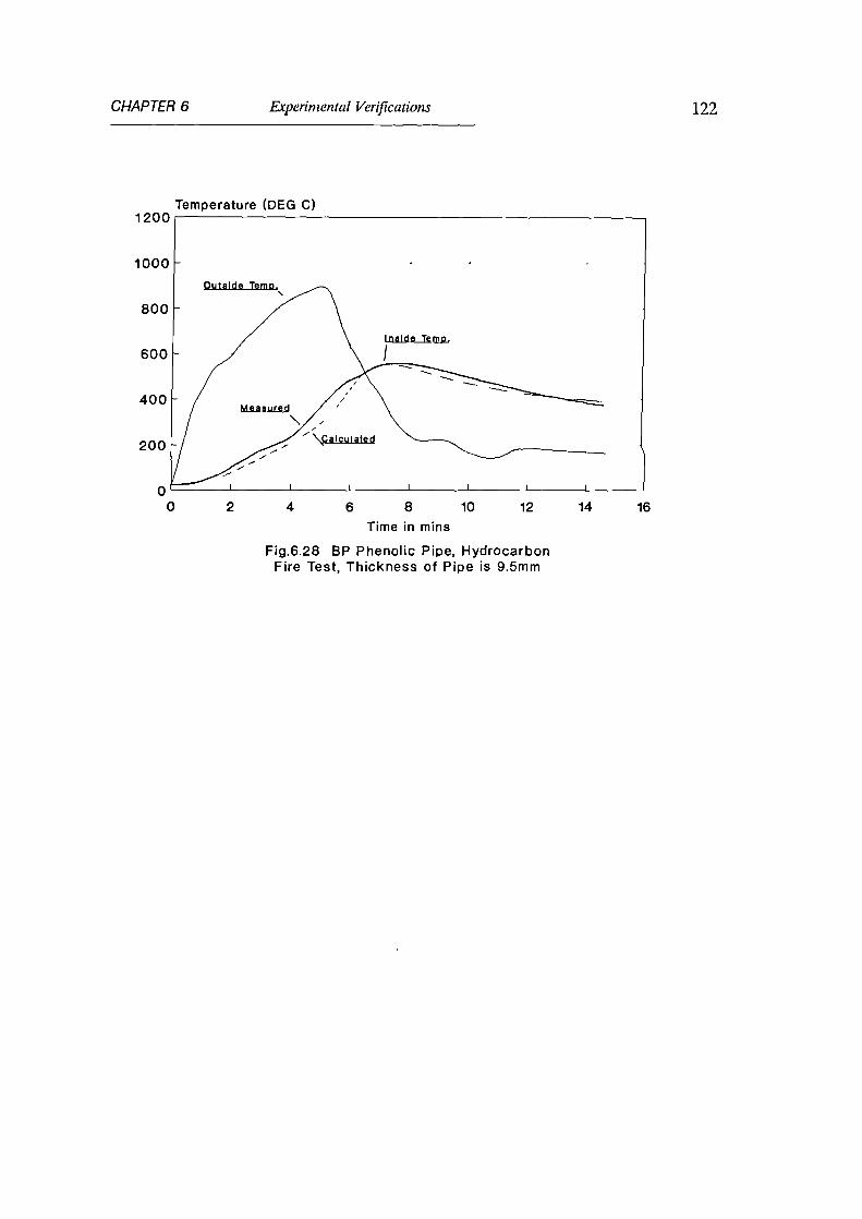
CHAPTER 6 Experimental Verifications 122
Temperature (DEG C)1200
1000
800
600
400
200
2 4 6 8 10
12
14
16
Time in mins
Fig.6.28 BP Phenolic Pipe, HydrocarbonFire Test, Thickness of Pipe is 9.5mm
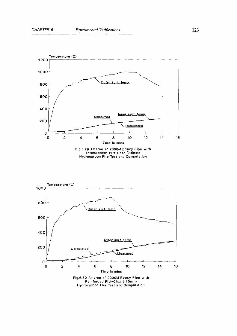
1200
1000
800
600
400
200
01614
\Outer surf temp.
Inner surf. temo,
Calculated\Measured
1000
800
600
400
200
1614
CHAPTER 6 Experimental Verifications 123
Temperature (C)
0 2 4 6 8 10
12Time In mine
Fig.6.29 Ameron 4 2000M Epoxy Pipe withIntumescent Pitt-Char (7.5mm)
Hydrocarbon Fire Test and Computation
Temperature (C)
0 2 4 6 8 10
12Time In mine
Fig.6.30 Ameron 4' 2000M Epoxy Pipe withReinforced Pitt-Char (11.5mm)
Hydrocarbon Fire Test and Computation

124
CHAPTER 7
Computer Program Development for FDM
Although, numerical heat transfer calculations can be performed by general
commercial packages, this would not meet the requirements of this study. The
first point is that calculations using such general purpose programmes will take a
considerable amount labour owing to the size of these programmes. Another
point is that if we want to study the particular behaviour of materials under fire,
such as moisture effect and decomposition of material, none of these
programmes have the required facilities, nor are the source codes available to be
modified. In general, the existing commercial software packages have not
included efficient fire - material models which usually tend to lag behind those
used for research purposes. It is therefore necessary to create an effective and
reliable program that can be executed within a PC environment, enabling a large
number of calculations to be made in a convenient way for this study.
Based on the finite difference formulae described before, a Numerical
Temperature Analysis Program - NTAP has been developed using the
FORTRAN language for one-dimensional analysis of heat transfer in either
Cartesian or polar coordinates, and two-dimensional analysis in polar coordinates.
The results obtained by using the program are the temperature profile of a
particular element of construction (panel, multi-layer panel or pipe) in a hostile

CHAPTER 7 FDM Programme Development 125
thermal environments of a specified intensity and time duration. NTAP is
designed to operate on a personal computer, although it can be executed on
other small computers or main frames. To make NTAP user friendly and
efficient, a simple data input by a pull-down menu management system and run-
time screen display have been established. In order to achieve this, the routines
and graphics facilities from the FTN77 (University of Salford) run-time library
were used. A high resolution graphics monitor with VGA screen type was
assumed and a mouse driver is required to make selections from the menus of the
program.
The main menu is shown across the top of the screen when the program is
running. It contains the following items: Configuration, Heat Source,
Properties, Settings and Options. The menu option Configuration is used
to specify the geometric dimensions of the element and the number of material
layers. The Heat Source selection is used to define the nature and duration of
the thermal impact which causes the structure to be heated. Five types of
exposed side boundary conditions are available, which included most of the
possible types of fire exposure. These are:
1). Cellulosic temperature-time curve[1.1];
2). Hydrocarbon temperature-time curve[1.1];
3). Actual furnace temperature-time history as recorded during a test;
4). Heat flux loading; It includes radiative and convective heat flux in
unit of KW/m2. The jet fire may be included in this category.
5). Actual exposed side surface temperature history.

CHAPTER 7 FDM Programme Development 126
The Properties selection is used to define the thermal and physical properties of
the materials. If the thermal conductivity and specific heat are temperature-
dependent, their relationship can be supplied to the program. These values are
adjusted according to the temperature and moisture content as the program is
running. Some default data for commonly used materials are held in the program.
An additional property library of further materials is to be included in a
database. The Settings option is used to adjust or alter the parameters used in
the modelling. The last menu item, Options, is used to command the program
to do a general task such as to quit the execution, display the previous results,
re-run the problem after alteration of the data and to start the new run. The
detailed explanation of how to use the menu system is given in a user's manual.
The initial time-step is set by the user based on the requirement for accuracy.
Firstly, this time-step is checked by program for the stability requirement. If the
time-step does not meet the requirement, the program automatically reduces the
time-step to half of its previous value until it meets this requirement.
In the principle, there is no limitation on the minimum thickness of the elements.
Sometimes the user may wish to run a similar problem many times. Typing in
almost same data repeatedly from menu selection could be tedious. The
program provides a solution to this in that the input data can be read from an
existing data file which can also be edited.
When the user runs NTAP, the curves of the numerical solutions are
instantaneously displayed on the screen. The experimental data can also be
shown on the screen at the same time for comparison. The data and graphic

CHAPTER 7 FDM Programme Development 127
results are also written to an output file and can be printed to provide a
permanent record. As with other finite difference packages, the program predicts
the temperature at every node and time step. Output of the nodal temperatures
can be done at a specified time interval. It is considered that the resulting
program is both stable and user-friendly.
The verifications of the performance of these computer programmes were carried
out during every stage of development. The details have already been described
in the previous chapters.
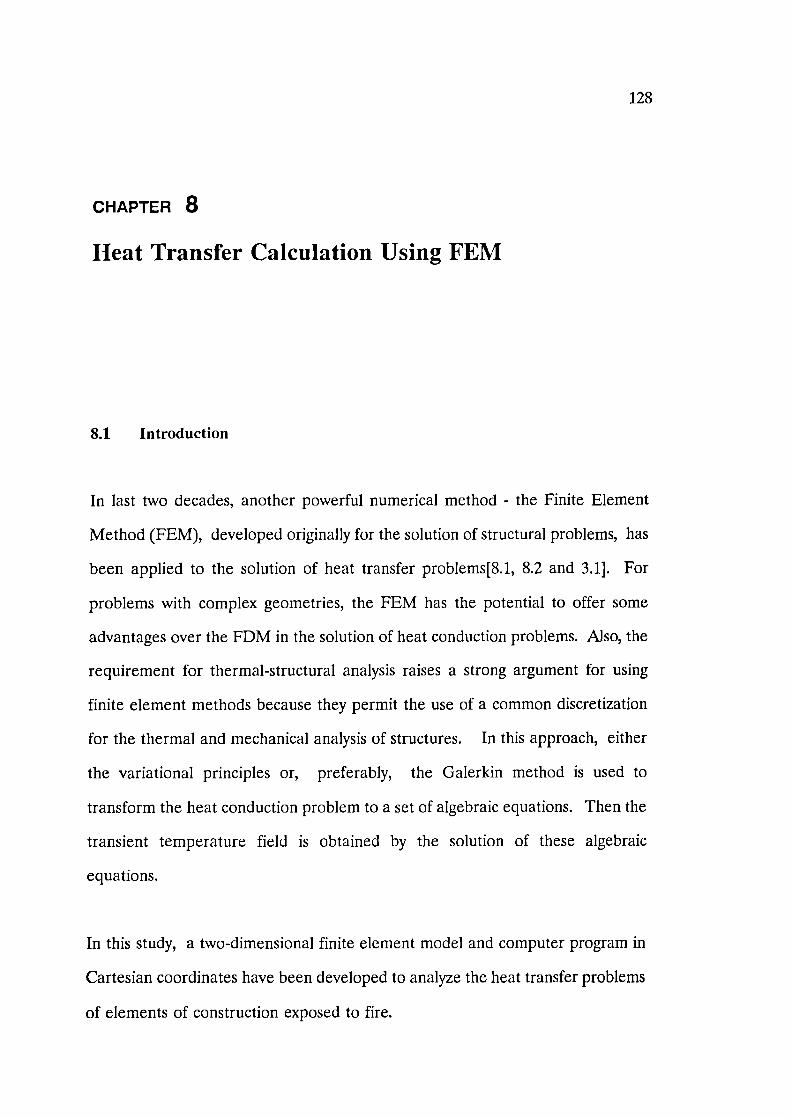
128
CHAPTER 8
Heat Transfer Calculation Using FEM
8.1 Introduction
In last two decades, another powerful numerical method - the Finite Element
Method (FEM), developed originally for the solution of structural problems, has
been applied to the solution of heat transfer problems[8.1, 8.2 and 3.1]. For
problems with complex geometries, the FEM has the potential to offer some
advantages over the FDM in the solution of heat conduction problems. Also, the
requirement for thermal-structural analysis raises a strong argument for using
finite element methods because they permit the use of a common discretization
for the thermal and mechanical analysis of structures. In this approach, either
the variational principles or, preferably, the Galerkin method is used to
transform the heat conduction problem to a set of algebraic equations. Then the
transient temperature field is obtained by the solution of these algebraic
equations.
In this study, a two-dimensional finite element model and computer program in
Cartesian coordinates have been developed to analyze the heat transfer problems
of elements of construction exposed to fire.

CHAPTER 8 Finite Element Methods 129
Since the principles of FEM for heat transfer problems are well known[8.1], the
details of its formulations will not be repeated here. A concise description of the
function of the developed FE program is presented in section 8.2, and a
representative problem is solved in sections 8.3 and 8.4 to show the capability of
FEM and the treatment of boundary conditions and moisture content.
8.2 Finite Element Computer Program Development
The developed 2-D FE program has a number of features that make it suitable
for the required purpose. The object structures may contain several materials
with thermal properties which vary with temperature. The heat transmission in
the enclosed voids by radiation and convection can be simulated as described in
section 3.3. Various boundary conditions can also be conveniently specified.
2The traditional usc. :. of the enthalpy concept in the FE formulation[3.__] was
abandoned in our program. It is believed that the introduction of enthalpy in the
formulation is not a necessity and may cause unnecessary complexity in the
programming and application.
In the present version of the program, two-dimensional four-noded rectangular
and three-noded triangular elements are used. By input of the main geometry
data, the generation of the finite element mesh has been automated. Graphic
output is available; ie, a display of the colour contours of temperature distribution
during the calculation process is provided. This provides a quick check for both

CHAPTER 8 Finite Element Methods 130
the element mesh and temperature profile.
Although this is a two-dimensional program, it can also deal with one-dimensional
problems. First, the check for one dimensional modelling was carried out.
The results given by the program for mineral wool and calcium-silicate panels are
quite consistent with the results which were given by fire tests and finite difference
modelling (see Figs.6.1 and 6.2).
8.3 Test Example:
Composite Concrete/Steel Deck Slab Exposed to Fire
For two-dimensional modelling, a series of careful standard fire tests for
composite deck slabs, conducted by P.W.Haar et al[8.3], were utilised to verify
the validity of the numerical analysis. The experimental arrangement used by
Harr is described in a supplement at the end of the thesis. The time-dependant
temperature distribution in the cross-section of composite concrete/steel deck
slabs exposed to standard fire condition was calculated. Furthermore, the effects
of temperature-dependent thermal properties of material, moisture content and
boundary condition have all received a detailed study.
The composite concrete/steel deck slabs normally span in one direction, in which
profiled steel sheeting acts as a permanent formwork and as reinforcement to the
concrete placed on top, as shown in Fig.8.1. A rapid increase in the use of this
form of construction in the UK has occurred since 1980. This is due in part to
the possibility of demonstrating adequate fire resistance without the necessity of
any added fire protection. The overall slab depth is usually 100 to 150mm, with

CHAPTER 8 Finite Element Methods 131
spans ranging from 2.5 to 4.0m. The steel sheet, with thickness between 0.7 and
1.5mm, is galvanised for durability. A number of fire tests have been conducted
carefully with the primary object of verification of the numerical models[8.3,8.4].
Unlike some other test reports, sufficient information was provided for the
numerical analysis to be replicated. Although R. Hamerlinck, L. Twilt and J.
Stark have already published a finite difference comparison for part of these
results[8.5], there is scope for refinement of their theoretical evaluations,
particularly with respect the treatment of the influence of the moisture content of
the concrete. In reference [8.6], a brief mention was given to the numerical
calculation for a similar problem. Nevertheless, it did not take into account the
effect of moisture which means that the over-predicted temperatures in concrete
were displayed.
The finite element meshes for the analysis of floor decks using the Holorib and
Prins profiles are shown in Figs.8.2 to 8.4, where both rectangular and triangular
elements are used. Because of the periodic nature of this form of construction,
only part of cross-section was used in the calculation. It was shown by
measurements made during testing [8.4] that the heat transfer in the longitudinal
direction of slab can be neglected. It follows that the temperature distribution
is not significantly influenced by the presence of any additional reinforcement in
the form of longitudinal bars or mesh.
The elements are assigned thermal properties of the materials which depend on
the average nodal temperature. These thermal properties are specified at a
number of temperature levels and are assumed to vary linearly between these.
Owing to the rapid temperature rise specified in standard fire conditions, a rather

h ( T) = 1 . 52 . ( Ta — T) 1/3 (8.1)
CHAPTER 8 Finite Element Methods 132
short time step is needed as the analysis proceeds. An explicit direct time
integration approach is therefore appropriate.
8.3.1. Boundary Conditions
In the tests, the slabs were positioned on the top of fire compartment with their
bottom face exposed to the fire. This represents a more severe situation than the
alternative with the fire burning above the floor. The temperature development
in the fire compartment was controlled to follow the ISO 834 standard time-
temperature curve as shown in Fig.8.5. A corresponding measured temperature
development in the fire compartment is used to generate an appropriate boundary
condition in the numerical modelling.
Both the radiative and convective heat transfer rates on the exposed and
unexposed sides can be described by equation(2.5). At the unexposed side of the
slab, a general formula for the free convection heat transfer coefficient in
horizontal plates is used, namely[8.4]
This is the simplified form of equation (2.15) for the current case. Alternatively,
only a constant value of h (8 W/m°C) was used in [8.5]. The configuration factor
F is 1 and emissivity of E is assumed to be 0.8 here.
At the exposed side of the slab, although the heat transfer coefficient h and the

CHAPTER 8 Finite Element Methods 133
resultant emissivity E are supposed to be constant, a distinction needs to be made
between the lower flange, upper flange and web because the heat transmission
to upper flange and web is partially obstructed. After first making reasonable
assumptions, these parameters were adjusted in order to improve the fit with the
test results. The values used in the analyses quoted later are summarised in
Tables 8.1 and 8.2.
Table 8.1. Super Holorib Specimens
Specimen 1,8 (If) 1,8 (uf,wb) 11 (If) 11(uf,wb)
h 25 15 25 10
EF 0.2 0.08 0.52 0.12
Table 8.2. Prins PSV Specimens
Specimen 6(If) 6(uf) 6(wb) 12(1f) 12(uf) 12(wb)
h 25 20 20 25 10 20
EF 0.2 0.12 0.14 0.52 0.14 0.38
Specimen 1 is Super Holorib 51/Hb=70mm (Fig.8.3) with the steel deck in place
and Specimen 11 is similar but without the steel deck. Specimen 8 is Super
Holorib 51/Hb = 90mm (Fig.8.4) with the steel deck. Specimen 6 is Prins PSV
73/Hb=70mm (Fig.8.2) with the steel deck and Specimen 12 is without steel deck.

CHAPTER 8 Finite Element Methods 134
In the above tables, 'If' refers to lower flange, `uf refers to upper flange and
`wb' denotes web.
8.3.2. Moisture Effects
The concrete slabs were made using normal-weight concrete B25. Although they
were subjected to a long period of natural and forced drying, they still contained
about 3% moisture content on the day of test. The levels of moisture content for
each specimen derived from the test report[8.3] are given in Table 8.3.
Table 8.3. Moisture Content of Test Specimens
Specimen 1 11 6 12 8
Moisture Content' 2.8 3.0 3.6 2.9 3.67
1 mass percentage of dry weight
It is well known that the heat transfer in moist materials is influenced significantly
by the moisture content. A same simple engineering approach 'is used as
described in Chapter 5. Although the distribution of moisture throughout thevs/
slab profile'is not necessarily uniform, it is assumed to be so in the current
numerical modelling.
v4-5According to this model, the moisture evaporation is assumed to take place
during a temperature interval, 100°C to 130°C. A = 1.5 in equation (5.2) is found

CHAPTER 8 Finite Element Methods 135
to give a satisfactory correlation with the experimental results for the cases
considered here.
Difficulties associated with numerical instabilities due to the abrupt variations in
C were overcome by choosing a gentle change occurring over the 30°CP
temperature interval in a way shown schematically in Fig.8.16.
Fig.8.16 The variation of DC p in a temperature interval
This was adopted solely to provide enhanced numerical stability and convergence
characteristics in the numerical calculations. The total energy which was needed
to evaporate the moisture was, in fact, not altered.
The thermal conductivity of concrete will be also influenced by the moisture
content. This will be discussed in the next subsection.

CHAPTER 8 Finite Element Methods 136
83.3. Thermal Properties of Materials
Since the thickness of the steel sheet forming the deck profile is small and its
thermal conductivity is high, the heat capacity and conduction resistance of the
steel deck may be neglected. Nevertheless, the emissivity of the galvanized steel
sheet has to be taken into account on the exposed side of specimens 1, 6 and 8.
This is the reason that the resultant emissivities on the exposed sides of specimens
1, 6 and 8 are lower than those for specimens 11 and 12 (see Tables 8.1 and 8.2).
The effective thermal conductivity of moist concrete will display an apparent
increase when the concrete is heated. Then the following relation between
conductivity and temperature shown in Table 8.4 is used for normal-weight
concrete (density = 2350 kg/m 3) with a moisture content around 3%. It may be
noted that the highest conductivity is at a temperature of 100°C.
Table 8.4. Thermal conductivity of concrete
Temperature (°C) 0 100 200 895 1200
Conductivity (W/m°C) 2.0 3.0 1.6 0.85 0.85
The specific heat for totally dried concrete is 900 J/kg°C at 0°C, and 1300 J/kg°C
at 1200°C. The actual specific heat of concrete with moisture content is
calculated by equation (5.3). The value of the final specific heat and conductivity
given by this procedure are consistent generally with the recommendations of the

CHAPTER 8 Finite Element Methods 137
ECCS[2.5].
8.4 Numerical Results and Comparisons
Numerical calculations were carried out for the five specimens mentioned above
using the finite element meshes shown in Figs.8.2 to 8.4. In order to obtain
coincidence between the positions of the thermocouples and element nodes, there
are slightly dimensional variations between the meshes for slabs with and without
the steel deck.
The comparisons of the observed and calculated time-temperature curves for
selected points are presented in Figs. 8.6 to 8.15. The 'No.' on the graphs
denotes 'Node Number' in the finite element mesh (see Figs.8.2 to 8.4). The
calculated results show good agreement with the test results. The calculation
time is just a few minutes with a PC 486 with time-step A t=2 sec.
The calculations for specimen 8 provide a particularly good confirmation of the
accuracy of the modelling. The shape of cross-section of specimen 8 is similar
to that of specimen 1, except that the concrete depth is increased to 90mm. All
input data for the numerical calculation for specimen 8 was therefore a copy of
that for specimen 1 except for the mesh generation and moisture content. An
excellent prediction was again obtained. This compares favourable with the 16
minute error in predicted insulation time found in[8.4].
In spite of the high thermal conductivity that was assigned to moist concrete at a

CHAPTER 8
Finite Element Methods 138
temperature around 100°C, the calculated temperature rise is still delayed in this
range as shown in Fig.8.10 and 14. This probably because the heat transmission
by diffusion of moisture was not fully considered. Nevertheless, the present
analysis gives better correlation with the test results than was obtained by the
authors of reference [8.4]. The total extra energy needed for vaporizing water
therefore seems to be correctly estimated.
Some discrepancies between the observed and calculated results occur on the
exposed side of slabs with steel sheets during the initial and final stage of testing.
In the initial stage, the relatively slow rise of measured temperature was
probably caused by the congestion of steam (Figs.8.8, 8.9, 8.12 and 8.13) while, irr
the final stage of the tests, the rapid rise of measured temperature might be a
consequence of debonding of the steel sheet (Fig.8.13). Cracks appearing in
concrete towards the end of fire testing also enhance the heat transmission in the
slabs.
The numerical results presented above show that an accurate prediction oi tine
temperature development in a composite concrete/steel deck slab exposed to fire
is available. Its use requires the determination of a number of parameters,
namely, the moisture content and its distribution, the energy needed for
evaporation, the value of the thermal conductivity under the influence of moisture,
and the actual heat input from the fire compartment.
For a prescribed time-temperature development, the parameters that determine
the radiative and convective heat loading from the fire compartment to the
exposed side of test sample differ from case to case. With the extremely

CHAPTER 8 Finite Element Methods 139
complicated turbulence of hot gas inside the test furnace, it is difficult to give the
accurate values of them in advance. The comparisons give here suggest that the
values of both the emissivity of the fire compartment and the heat transfer
coefficient (Eq.(2.5)) are high at the start of the test when the temperature is
increasing rapidly. They then decrease as the rate of temperature increase
decreases. On the other hand, the galvanized steel sheet shows low emissivities
for low temperatures. When the temperature exceeds 400°C, however, the zinc
layer melts and surface blackens with the result that its emissivity increases. For
the combination of these two effects, a constant resultant emissivity appears to
provide a reasonable assumption for the radiative heat exchange between the steel
sheet and the fire compartment. For the concrete slabs alone, specimens 11 and
12, although a constant value was chosen for simplicity, the numerical results
will be improved if variable emissivity is used (Fig.8.10).
The use of a high thermal conductivity for moist concrete around 100°C gives a
good predictive of the behaviour as the moisture evaporates. An accurate value
of the extra energy needed for vaporization is also important.

re-entanl
trapezoidal
ackitional reinforcatnant
651 2 346 e
_
17
\\\
-
12
18
143
30
38
42 —
7
13
19
CHAPTER 8 Finite Element Methods
140
Fig.8.1 Typical composite concrete/steel deck slabs [8.2]
Fig.8.2 Finite element mesh for Prins PSV 73

J
aoCo
CHAPTER 8 Finite Element Methods 141
I0
to
am
ai•
P.
V
03
oa
.-
...
..-
011 03 V oo.... •,• 04 co
.-a- 03
.- •
,..011rn
lpWCV
10
10
04
41:;
p-
.1.
Co
•s
n•n• • 04
n
r... CI C0••

\Compartment 2
180 834
Compartment 1
1200
1000
800
600
400
200
No.42
No.30
--..—
-\Calculated
-
_histIO
No.12_
I 1 i I I 1 I )
142CHAPTER 8 Finite Element Methods
Temperature (DEG C)
1200
1000
800
600
400
200
25 50 75 100 125 150 175 200
Time in mins
Fig.8.5 The Measured Temperature inFire Test Compartment 18.21
Temperature (DEG C)
20 40 60 80 100 120 140 160 180 200
Time in mins
Fig.8.6 The Comparison of Calculatedand Measured Temperature Distribution
Prins PSV 73 (without steel sheet)

No.42Measured
\, \ Calculated
1200
1000
800
600
400
200
-
-
_
-
-
CHAPTER 8 Finite Element Methods
Temperature (DEG C)
143
20 40 60 80 100 120 140 160 180 200
Time in mins
Fig.8.7 The Comparison of Calculatedand Measured Temperature Distribution
Prins PSV 73 (without steel sheet)
Temperature (DEG C)
20 40 60 80 100 120 140 160 180 200
Time in mins
Fig.8.8 The Comparison of Calculatedand Measured Temperature Distribution
Prins PSV 73 (with steel sheet)
1200
1000
800
600
400
200

1200
1000
800
600
400
200
0
1200
1000
800
600
400
200
0
144CHAPTER 8 Finite Element Methods
Temperature (DEG C)
0 20 40 60 80 100 120 140 160 180 200
Time in mins
Fig.8.9 The Comparison of Calculatedand Measured Temperature Distribution
Prins PSV 73 (with steel sheet)
Temperature (DEG C)
o 20 40 60 80 100 120 140 160
Time in mins
Fig.8.10 The Comparison of Calculatedand Measured Temperature Distribution
Holorib 51/HB •70mm (without steel sheet)

1200
1000
800
600
400
200
0
145CHAPTER 8 Finite Element Methods
Temperature (DEG C)
0 10 20 30 40 50 60 70 80 90 100 110 120 130 140 150 160
Time in mins
Fig.8.11 The Comparison of Calculatedand Measured Temperature Distribution
Holorib 51/Hb ,70mm (without steel sheet
Temperature (C)1200
1000
800
600
400
200
00 20 40 60 80 100
120
140
160
Time in mins
Fig.8.12 The Comparison of Calculatedand Measured Temperature DistributionHolorib 51/Hb•70mm (with steel sheet)

1200
1000
800
600
400
200
0
1200
1000
800
600
400
200
0
CHAPTER 8 Finite Element Methods 146
Temperature (C)
0 20 40 60 80 100
120
140
160
Time in mins
Fig.8.13 The Comparison of Calculatedand Measured Temperature DistributionHolorib 51/Hb-70mm (with steel sheet)
Temperature (C)
0 20 40 60 80 100 120 140 160 180 200 220
Time in mins
Fig.8.14 The Comparison of Calculatedand Measured Temperature DistributionHolorib 51/Hb-90mm (with steel sheet)

_
-
147CHAPTER 8 Finite Element Methods
Temperature (DEG C)
No.19Measuredn ----- \Calculated
plo.13
I40.7
Q,Li.
1000
800
600
400
200
_
20 40 60 80 100 120 140 160 180 200 220
Time in mins
Fig.8.15 The Comparison of Calculatedand Measured Temperature DistributionHolorib 51/Hb •90mm (with steel sheet)
148
CHAPTER 9
Experimental and Computational Approaches
In the past, considerable research has been done and considerable advances have
been made in the determination of the fire resistance of components of
construction. Nevertheless, there is still a lack of appropriate regulations and
design codes concerning the use of some composite materials such as GRP.
Moreover, one of the major recommendations which was strongly endorsed by
the Lord Cullen report[9.1] on the Piper Alpha disaster, which occurred on 6 July
1989 and claimed 167 lives, was that the industry should move away from a
prescriptive, mechanistic approach to safety requirements, to those of a goal-
setting nature which ensure an adequate response. Then the one major problem
often confronted by designers and product developers is: " which is the best and
cost-effective way to satisfy such guidance? "
Currently, there are two fundamental ways to investigate the fire performance of
a structure, namely experimental and computational approaches. Both the
advantages and disadvantages of experimental and computational approaches are
discussed in this chapter. The main conclusion is that the best strategy to carry
on the optimisation of design for fire critical applications, is to obtain synergy
between the experimental and theoretical approaches. In fact, both approaches
are complementary to each other in nature.

CHAPTER 9 Experiment and Computation 149
9.1 Fire Resistance Tests
Although fire tests for materials and structures could include consideration of the
following aspects: fire resistance, fire propagation, heat release and smoke
release rate; fire resistance is the main concern of this thesis. As stated above,
the primary objective of the fire resistance test method is to determine the length
of time that an assembly of construction will satisfy certain criteria related to its
intended function under exposure to the test conditions. The fire resistance test
is used basically for three purposes:
to be able to claim fire resistance for a given construction and
hence to have it accepted by the regulatory bodies
. to assist with the development of new products and systems
. to establish the essential parameters to predict the fire behaviour
of elements of a structure.
Furthermore, fire resistance tests can be divided into the following categories:
full-scale standard tests, small-scale 'standard' tests and whole structure tests.
The required fire resistance rating is assigned by the building codes for various
portions of the assembly, depending on its relative significance to the overall
structural stability or the importance of it retains its function. The size of the
element for a full-scale standard test, for example for a vertical separating
element according to BS476:part 20[1.1], should be a full sized element of
building construction or if it exceeds the size that can be accommodated by the
furnace, the minimum size of element exposed to the heating conditions in the

CHAPTER 9 Experiment and Computation 150
furnace should be 3m high by 3m wide. These tests therefore require
considerable facilities, manpower, and material to conduct and thus they can be
expensive. The testing costs for a large research program can be appreciable
since many samples may be needed to evaluate alternative protection materials
with various thicknesses and construction details. Another problem is that the
number of existing furnaces which meet the size requirement is also limited.
However, the fire resistance rating is a basic property for which all products in
the market are tested, and it gives the user or specifier the first criterion for
selecting a suitable product.
The indicative small-scale test, which replicates the particular test specifications
but on a smaller sample, provides an alternative scheme for fire testing. It is
usually preferred for the research activities involved in developing a fundamental
understanding of the behaviour of a component and is the procedure used in this
thesis. Obviously this test method greatly reduces the costs and time. This
enables sensible assessments and indications for actual fire performance to be
made which is very useful in the development of a new material or in the
comparative evaluation of existing materials. It can also provide the data for the
calibration and validation of theoretical models.
Although the standard tests have their limitations, such as the consideration that
the applied thermal procedure may not represent an actual fire, they certainly
establish the points of comparison for the overall risk and behaviour, and provide
a measure of the relative performance of structures and materials within the
capabilities of fire testing furnaces. Therefore, they are the prescriptive testing
which is required in many countries. Full-scale tests can also supply the

CHAPTER 9 Experiment and Computation 151
information necessary for the development of reliable small-scale tests.
Once the confidence has been established in the design of a structure on the basis
of material and element fire tests, a whole-scale compartment test might be
needed to prove its performance conclusively with the provision of realistic fire
conditions. Sometimes, realistic dimensions are important in evaluating certain
effects, for example, the effects of continuity in continuous beams or of the
degree of fixity in beam-to-column connections, the effects of static loads on
structural elements exposed fire and the effects of specimen dimensions. In any
case, it is the real fire attack that has to be anticipated and to be withstood by
fire protecting structure. A whole-scale experiment may be the only resort for
some very complicated and critical cases, and most engineers have more
confidence in the results of such tests.
In these tests, the treatment of fire as a load condition requires that the fire type,
location, geometry, intensity and heat flow characteristics be defined. It is clear
that the design of this sort of experimental arrangement, which is a true
representation of the actual hazard, is by itself a fairly difficult process. It will
depend on the actual circumstances and requirements, and may require an
empirical approach to be designed by fire experts. Obviously, to test the whole
structure under realistic fire condition is also overwhelming costly.
Fire tests can also be classified according to the type of fire that they represent.
Typical examples are cellulosic furnace fire tests, cellulosic room fire tests,
hydrocarbon furnace fire tests, hydrocarbon jet fire tests and pool fire tests.
Except for the furnace tests, there are no well established individual standards for
CHAPTER 9 Experinzent and Computation 152
these tests.
Every fire test, if reproducible, is satisfactory for its own configuration and
scenario. However, it is unrealistic to expect that one small-scale test will
completely describe the fire risks of the real world. This problem exists even in
large-scale tests are used. Yet, properly interpreted small-scale tests offer the
most practical and economically reasonable method of evaluation the fire
behaviour of materials. Therefore, problems have arisen in using the results from
specific tests to predict fire behaviour in the unlimited configurations found in the
real world.
9.2 Computational Approach
The ever increasing cost of fire tests is contrasted to the failing costs of computer
software and hardware. The time scale associated with the running of a
computer programme can be significantly less than the time required to set up
and execute a fire test of the same problem. In addition, an advantage of a
computational analysis is that it enables the performance of a passive fire
insulation material to be assessed for applications which may deviate significantly
from those modelled in the standard tests. Numerical analysis can offer greater
flexibility in the choice of geometries, sizes, materials and boundary conditions,
then as a consequence, increasing the opportunities for flexibility in design. It
gives the designer more control over the performance of the system and a
considerable reduction in the need for involved fire tests. The modelling of

CHAPTER 9 Experiment and Computation 153
different possible alternatives by computational technique is of great help during
the planning stage.
The prime objective in passive fire protection is to reduce the temperature rise
in the components during the fire. The computational thermal models allow
the prediction of the temperature increase throughout a structure subject to a
heat flux. The constructional design can then be easily established for a range of
required thermal insulation at an appropriate thickness for particular heat loads
and fire durations.
Nevertheless, it is useful to be aware of the drawbacks and limitations of the
computational method. The limitations of the computational approach are that
some processes are not easily modelled and that the accuracy of a model depends
on the assumptions and approximations made in formulating it and in the material
properties adopted. In detail, the applicability of the thermal model is
dependent upon following factors:
a. A precise representation of the heat loading with time.
b. Thermal properties and pyrolysis data, including the:
1. Thermal conductivities of the material at various temperatures
(and moisture contents).
2. Specific heat capacities of the material at various temperatures.
3. Emissivity of the surfaces at various temperatures.
4. Kinetic parameters A and E A, as defined in Chapter 4.
c. Energy losses or gains associated with chemical reactions or changes of
state that may occur to materials at elevated temperature.

CHAPTER 9 Experiment and Computation
154
If these requirements are fulfilled, then the performance of a particular element
of construction subjected to a fire test will not be difficult to determine by a
computational approach.
Over the last two decades, research bodies in many countries have studied the
behaviour of construction elements in real fires and in fire resistance tests, and
thus obtained data on the effect of high temperatures on the properties of
material. This has consequently paved the way for the possibility of computing
fire resistance as part of the normal design process. Many national and
international committees are now engaged in refining procedures which can be
adopted by professional bodies, code preparing organizations and regulatory
authorities. Given the common research effort, the tendency to replace some
fire tests with fire-safety engineering calculations is now being accepted at official
and legal levels. For instance, the European Convention for Constructional
Steelwork published its European Technical Notes on a calculation method to
determine the fire resistance of centrally loaded composite steel concrete columns
exposed to the standard fire[2.5], and the 1992 Eurocodes contain clearly
separate chapters on structural fire design where calculation procedures are
accepted[9.2]. An American Concrete Institute Committee 216 even offered the
following revising statement to AC! 216R-81 'Guide for Determining the Fire
Endurance of Concrete Element' [9.3]: " As shown in the previous sections of
this Report, performing such (fire endurance) tests is not necessary for a large
number of concrete elements. Information on their fire endurance can be
derived by the application of calculation procedures based on heat flow
studies and structural analyses, and on the knowledge of the behaviour of
concrete and steel at elevated temperatures, rather than by fire test."
CHAPTER 9 Experiment and Computation 155
Nevertheless, the evaluation of the fire behaviour of components of construction
under real fire condition is a complex process. Risk depends not only on the
intrinsic properties of the material but also on the amount of material, its
configuration, and its exposure. Risk also depends critically on the environment
and usage. Research in numerical modelling has the potential to provide a more
fundamental understanding of heat transfer and fire resistance problems. In
principle, numerical modelling offers a rigorous framework because all the
interacting processes, if known and capable of accurate quantitative description,
can be included.
In order to obtain the desired level of accuracy and predictability, the fire test
arrangements also need improvement in order to provide more precise data to
verify and elaborate the numerical models. The harmonization of standard test
methods for different countries is also demanded. Efforts should be made to
standardize the construction of test furnace such as to dimension, materials used,
fuel, burner and exhaust arrangement, aiming at reducing the differences between
the various furnaces.
Looking ahead, the development of rigorous and intelligent computational tools
incorporating fire parameters to complement or replace the furnace tests will be
continuously pursued, with the aim of maturing the simplified design guidance to
meet the requirement of stipulations and even the prediction of the durability in
real fire scenarios. This is believed to be of considerable long-term value to the
industry.

156
CHAPTER 1 0
Summary and Conclusions
10.1 Present Study
Major fires usually cause severe structural damage, even in areas remote to the
fire area. Fire could lead to partial or total collapse of an industrial installation
or domestic building resulting in loss of life, property and/or environmental
pollution, as happened in the North Sea Piper Alpha disaster. Considerations
should then be given in the design of the structure and its protection in order to
minimize the effects of these events. Preventive measures have historically been,
and will continue to be, the most effective approach in reducing the probability
of spread of a fire and the resultant consequences of the conflagration.
The industries have long relied on prior experience to provide 'expert judgment'
for evaluating fire hazards. This has worked reasonably well for traditional
materials used in the traditional manner, but when new materials are used or old
materials are used in new ways, hazards may be developed which are difficult to
anticipate if there is a lack of suitable analytical methodology. It is desirable that
the fire safety of products, including those using advanced composite materials,
should be treated by the same good engineering practices as are used for the
determination of strength and performance.

Chapter 10 Suninzary and Conclusions 157
The determination of the temperature distributions in the components of
construction, due to fire, is critical for the valuation of the passive fire protection
required in the construction. This thesis presents a methodology to study such
events, which involves a combination of theoretical, numerical and experimental
approaches.
The design of building elements for a prescribed level of fire safety can be made
based on established engineering principles. Prediction of their fire endurance
can also be derived by the application of analytical procedures, rather then by
fire tests only. The complexity of the governing equations generally allows
analytical solutions to be obtained only for very simple cases, making it necessary
to use numerical techniques for most problems of practical interest. With the
expansion of the capability of personal computer and using computer codes, this
approach is becoming increasingly more practical. The growing need to optimize
fire protection systems has made it imperative to simulate the relevant thermal
transport phenomena numerically, since experimentation is usually too involved
and expensive. There has been a phenomenal increase in the use of
computational methods for heat transfer problems, as a result of their low cost,
remarkable speed, detailed and complete information. However, available
analytical and experimental results are of considerable importance in checking the
accuracy and validity of numerical results.
In the principle, the computational thermal models developed in this thesis can
be used for the design of the loadbearing and non-loadbearing elements of
construction for prescribed level of fire safety. However, for loadbearing
components, their deflection should be included in the calculation, provided that

Chapter 10
Sunimaly and Conclusions 158
the mechanical properties of the material at elevated temperature are known.
General speaking, there are three obstacles to the numerical heat transfer analysis
for an element of construction subject to fire. The first problem is to determine
the heat exchange between the outer surface of the element and the fire
environment. This includes the determination of the heat loading from the fire
and environment, the heat loss from the structure, the view factor and the
emissivity. The next question concerns that the inadequate information on the
thermal properties of material at elevated temperatures. The third problem is
the shortage of knowledge of the various processes that affect the heat transfer
during exposure to fire, such as moisture migration and material decomposition.
All of these problems and their influences have been investigated in this study.
Simulated cellulosic and hydrocarbon fire tests have been conducted for various
materials and configurations. Emphasis was laid on the development and
verification of one and two-dimensional finite difference and finite element
thermal models.
With the advances in material science, sandwich construction is increasing its
application in fire resistant structures. In Chapter 2, the explicit finite difference
formulations for multi-layer panels were derived. The spatial intervals for FD
analysis of the different material layers could be unequal. The realistic boundary
conditions on the exposed and unexposed sides of the panel have been formulated
from the normally established physical equations. The heat transfer coefficient
for convection and resultant emissivity for radiation are the decisive factors within
the formula.

Chapter 10 Summary and Conclusions 159
A similar treatment for the multi-layer pipes was described in Chapter 3. It also
includes the two-dimensional finite difference formulations for pipes and the
treatment of internal heat exchange.
One of the major concerns of the architect and engineer using materials
incorporating plastics resin in the construction industry is the problem associated
with fire. In Chapter 4, a blend of experimental, theoretical and numerical
techniques was used to exploit predictive capabilities for the thermal response of
fire resistant polymer composites. The approach included the correlation of
thermophysical properties as function of temperature and stage of decomposition.
These correlations are then used in a one-dimensional numerical model, with a
formulation based on major physical and chemical processes occurring in a
decomposing and expanding polymer composite. The initial attention was
focused on the performance of GRP laminates and pipes. The various factors
which influence the heat transmission were investigated in detail.
One discovery as a consequence of fire tests on GRP laminates is that the effect
of internal convection may be neglected due to the poorer contact between the
liberated gas and the fragments of the carbonaceous char.
Another finding is that the interlayer delamination is an important factor which
affects the fire resistance of woven roving glass-fibre/phenolic laminates. A new
model for delamination in a phenolic laminate was therefore proposed, and a
good agreement was then obtained between the theoretical prediction and
experimental measurement.

Chapter 10 Sumnzwy and Conclusions 160
Depending on the type of problem under consideration, either the heat absorbed
or the heat released by combustible materials in a fire environment may be critical
respectively. When the flashover point of a fire in a construction is considered,
the heat generated by the combustion of the volatiles should be known.
Conversely, if the fire resistance of a component in a standard furnace test is
simulated, the amount of absorbed heat for decomposition is important. In fact,
both the heat absorbed and heat released are two key factors in the progress of
a fire. They will determine the probability of ignition, fire spread and sustaining,
and the decay of a fire.
The characteristics of the intrinsic thermal properties and the kinetic parameters
of pyrolysis on heat transfer were discussed in Chapter 5. The values of these
parameters which were used in the numerical modelling were listed. The
significant influence of moisture content on thermal conductivity and specific heat
capacity was investigated in considerable detail. A new treatment for the
moisture influence on heat transmission was then proposed and the experimental
confirmation was given.
Chapter 6 provided the experimental verification of the theoretical analysis and
numerical calculation for various 'traditional' and innovative composite materials.
The dimensions and constitution of the specimens were described and the
comparisons of numerical and experimental results were performed.
On the basis of the developed models, a number of use-friendly finite difference
computer programmes were written. The description of these programmes was
outlined in Chapter 7. These programmes are capable of evaluating the

Chapter 10 Summary and Conclusions 161
temperature distribution history of various construction components under fire
impingement. Pre- and post-processors were integrated into the programmes
which allow fast and use-friendly input/output operations. The programmes
provide a convenient tool for the validation of innovative theoretical models and,
at same time, a valuable means for fire safety design.
Heat transfer analysis may be expected to be able to model realistic
environmental boundary conditions, to represent complicated geometry and to
analyze a variety of materials. Of the two, the finite element method is believed
to be superior to the use of finite difference methods. In Chapter 8, a two-
dimensional finite element model for the heat transfer problem was accomplished.
The verification of its performance was carried out by means of a practical
example: namely a composite concrete/ steel deck slab exposed to fire using data
from tests conducted by other researchers. An excellent agreement was obtained
between the computational results(which incorporated the proposed model for
moisture effects) and the experimental measurements.
In Chapter 9, the general issues about the role of experimental and computational
approaches in fire safety study and design were highlighted.
The following main conclusions can be drawn from this work:
1. In order to address the fire resistance problem effectively, the optimal
approach is the combination of experimental and computational schemes.
2. Due to the aforementioned advantages of numerical modelling, the

Chapter 10 Summary and Conclusions 162
influence of each parameter on heat transmission can be more readily
assessed by computer. This enables both the controlling authorities and
designers to arrive at solutions which represent the optimum level of
protection commensurate with the risk.
3. The discussion about the relative merits of computational analysis and
experimental investigation is not aimed at recommending computation to
the exclusion of experiment. Both of them have their own place. The
sequence of fire testing should be in an ordered progression leading from
small scale laboratory testing, then gradually increasing in scale and
complexity.
4. In the development of the computational models, it should be born in mind
that they should easy to apply. The simplest model can be accepted which
has the ability to predict the thermal behaviour with an acceptable
accuracy and which minimizes the number of variables in the model.
5. With the provision of the requisite parameters, it is possible to provide an
accurate temperature distribution for elements of construction subjected
to a specified fire environment. The thermal properties of insulating
materials can be evaluated by comparisons with the results obtained from
the necessary fire tests and computer simulations. Once confidence is
obtained, the computational programme can analyse and optimise the
passive fire protection of any profile for any boundary condition and fire
exposure. It can also assist and guide the experimental work.
Chapter 10 Summary and Conclusions 163
6. The explicit finite difference method was proven to be a simple and
effective method to solve the heat conduction problem in elements of
construction .
7. A number of successful comparisons between numerical analysis and test
results have been obtained in this study, and additional insight into the
heat transmission mechanism on a variety of elements of construction has
been offered. Based on the results of this thesis, two scientific papers
have been presented in distinguished international forums[5.19,10.1], and
a further three papers are going to be published[10.2-4].
8. With the consideration of the moisture content, although the presence of
moisture will raise the apparent thermal conductivity of the material, the
energy needed to drive off the water, which could be either physically or
chemically trapped in the material, is of considerable significance. Then
the time needed to elevate the temperature on the unexposed side of a
component heated until the insulation criterion is exceeded is extended
significantly and this is of great benefit for its fire resistance.
9. Although the delamination in woven roving glass-fibre/phenolic laminate
at high temperature will be beneficial for heat insulation, it may be
unwelcome since it will wreck the structural integrity and reduce the
mechanical strength. In order to avoid this, some property improvements
should be made for phenolic resin to relieve this effect.
10. Whereas the development of scaled down bench mark tests will not totally

Chapter 10 Somoza?), and Conclusions 164
eliminate the need for full scale testing, it will allow quick and low cost
screening of candidate materials. The laboratory-scale technique which
was employed in this study is suitable for calibrating the theoretical models.
11. Most previous tests were not initially designed to provide an analytical
basis for computing, and consequently difficulties have been experienced
in completely correlating the calculated and the experimentally obtained
performance. The standard fire test methods should be improved by
establishing the precise properties of the materials being subjected to the
test and by applying additional data to the mathematical model, which will
then facilitate interpolation and extrapolation of these data. It will also
be of great help for the wide acceptability of the analytical approach[10.5].
12. With the advent of computers in design offices and their use for normal
design purposes, it is inevitable that similar techniques should be
considered for fire design. The completion of this thesis is expected to
form a necessary step towards this end. The computation of the fire
resistance of some types of elements of construction has become a reality
and it is only a matter of time before these methods will be widely used by
the industry.
10.2 Future Development
CV% trA k)Orka,rvk
Standard fire resistance tests and their computational simulation play sole

Chapter 10 Summary and Conclusions 165
in fire engineering. Both the temperature of a fire and its heat flux should be
considered before making a fire safety judgment because there is no accepted
correlation existing between the temperature of a fire and its heat flux falling on
the surface of a structure. Unfortunately, the existing inventory of various fire
resistance standards have a serious deficiency at this point. The temperature in
a fire testing furnace is usually controlled in accordance with these standards.
However, defining temperature-time characteristics is necessary but not sufficient
as the sole characteristic for determining the thermal loading for a construction
element exposed to a fire, as shown in Eq.(2.5). For a prescribed temperature-
time curve, the convection and radiation heat transfer from the fire to a specimen
can vary considerable from one furnace to another[10.5,10.6]. Ideally, it would
be preferable to control furnaces to regulate the total heat irradiation received at
the surface of the test specimen. Unfortunately, there are serious instrumental
difficulties inherent in such a scheme.
Accordingly, an important development will be concerned with the instrument
improvement which can precisely measure of heat flux received by the structural
element under test. If this does not work, alternatively, the following proposal
might be worth exploring. The idea is that with the use of numerical techniques
and the measurement of the temperature profile on a thermally stable sample
whose properties are well known, the irradiation provided by the furnace might
be computed by the methods described in this thesis. The main advantage of
such data is to enable an accurate assessment to be made of heat transmission
from the fire to the construction. This would allow furnace test results to be
correlated to a standard heat impingement. In the long term, uniformity in the
method of controlling exposure conditions for different fire test environments

Chapter 10 Sum:my and Conclusions 166
needs to be pursued.
Other further subjects could be:
1). Additional experimental verification of pipe modelling. Tests on more
pipes and their joints are needed to check the numerical programme.
These should also include two-dimensional heat loading and pipes filled
with stagnant and flowing water.
2). Extra verification of moisture modelling with large hygroscopic panels with
impervious skins. The interrelation between bench-scale and full-scale fire
test methods is also needed to be further investigated.
3). The assumption of perfect contact between the interface of two material
layers may cause some errors, as shown in Specimen 7 in Chapter 6.
Although considerable amounts of theoretical and experimental work have
been done on the prediction thermal contact resistance, it appears that
the reliable results for practical use are still those that have been
determined experimentally[5.19]. Based on experimental results, an
empirical formula might be added to the existing numerical modelling.
4). Continued development work on the three-dimensional model and
programme will permit the analysis of the problems with more complicated
configurations, such as joints and concrete with spalling. Identifying the
most effective numerical procedure to solve the corresponding nonlinear
equations is also demanded.
Chapter 10 Summary and Conclusions 167
5). More accurate thermophysical properties of various materials are required.
The nonlinear regression method might be useful to tune these properties
from experimental data[10.7-8]. Some data, for the instance heat release
rate of combustible materials, might be procured through some special
instruments, such as the cone calorimeter[10.9].
6). For decomposing materials, a study of the effects of the assumption of
local-thermal equilibrium and internal convection on the overall response
might be needed. More work could be carried out to verify the extended
model for other materials, such as timber.
7). As was outlined previously, one main drawback in the all existing fire
resistance standards is that all of them specified the severity of fire in
terms of temperature. Actually, the fire severity does not solely depend
on the temperature of the fire. The more important parameter is how
much heat flux is irradiated onto the surface of the structure. The
determination of the emissivity and heat transfer coefficients for standard
and actual fire environments should be further explored.
9). The determination of the mechanical responses of structural element under
fire impingement is also very important in many situations. The
interrelated influence of thermal and mechanical behaviours should be
considered at this stage. As the temperature field and the mechanical
properties of the material at elevated temperature are known, the
mechanical behaviour of the structure can be determined by using
commercially available finite element packages.

168Chapter 10 Summary and Conclusions
List of Main References
[1.1] BS476:Part 20: Fire Tests on Building Materials and Structures.British Standards Institution, 1987 and AMD 6487, April 1990.
[1.2] International Organization for Standardization: InternationalStandard ISO 834, First edition, 1975.
[1.3] Babrauskas, V., and Williamson, R.B.: The Historical Basis of FireResistance Testing -Part I., Fire Technology, 14,184-194, 1980.
[1.4] Babrauskas, V., and Williamson: The Historical Basis of FireResistance Testing -Part II., Fire Technology, 14,304-316, 1980.
[2.1] Croft, D.R. and Lilley, D.G.: Heat Transfer Calculations UsingFinite Difference Equations, Appl. Sci. Publ., London, 1977.
[2.2] Orivuori, S.: Efficient Method for Solution of Nonlinear HeatConduction Problems, Int. J. Num. Meth. Eng.,14,1461-76,1979.
[2.3] Wrobel, L.C.: A Novel Boundary Element Formulation for
Nonlinear Transient Heat Conduction, Numerical Method inThermal Problems, Ed. R.W.Lewis and K. Morgan, vol V.,1987.
[2.4] Holman, J.P.: Heat Transfer, 7th Edition, McGraw-Hill PublishingCompany, 1990.
[2.5] European Convention for Constructional Steelwork: Calculation ofthe Fire Resistance of Centrally Loaded Composite Steel-Concrete Exposed to the Standard Fire. First Edition, 1988.
[2.6] Thring, M.W.: The Science of Flames and Furnaces, secondedition, Chapman & Hall LTD, 1962.

LIST OF REFERENCES
[2.7] Incropera, F.P. and De Witt, D.P.: Findamentals of Heat and MassTransfer, third edition, John Wiley & Sons, 1990.
[2.8] Fletcher, J.D. and Williems, A: Emissivities of Ceramic FibreLinings for High-temperature Furnaces, J. of the Institute Energy,
p377-380, V57, 1984.
[3.1] Ozisik, M.N.: Heat Transfer, McGraw-Hill, New York, 1985.
[3.2] Sterner, E. and Wickstrom, U.: TASEF - Temperature Analysis ofStructures Exposed to Fire, Swedish National Testing Institute, SPReport 1990:05.
[3.3] McAdams, W. H.: Heat Transmission, McGraw-Hill Book
Company, 1954.
[3.4] Siegel,R. and Howell, J.R.: Thermal Radiation Heat Transfer, thirdedition, Hemisphere Publishing Corporation,1992.
[4.1] Bamford, C.H., Crank, J. and Malan, D.H.,The Combustion ofWood, Part 1, Cambridge Phil, Soc. Proc., Vol.42, p166-182,1946.
[4.2] Matsumoto,T., Fujiwara,T. and Kondo,J.: Nonsteady ThermalDecomposition of Plastics, Twelfth Symposium (International) onCombustion, The Combustion Institute, p515-521, 1969.
[4.3] Kung, H.C.: A Mathematical Model of Wood Pyrolysis,Combustion and Flame, Vol 18, p185-195, 1972.
[4.4] Griffis,C.A., Masumura, R.A. and Chang, C.I.: ThermalResponspone of Graphite Expoxy Composite Subjected to Rapid
Heating, J. of Composite Materials, Vol 15, p427-442, 1981
[4.5] Kanury,A. M. and Holve,D.J.: Transient Conduction with Pyrolysis(Approximate Solutions for Charring of Wood Slabs), J. of Heat
Transfer, Vol.104,p338-343, 1982.
169

LIST OF REFERENCES 170
[4.6] Henderson,J.B., Wiebelt,J.A, and Tant,M.R.: A Model for theThermal Response of Polymer Composite Materials withExperimental Verification, J. of Composite Materials, Vol.19, p579-
595, 1985.
[4.7] Fredlund, B.: Modelling of Heat and Mass Transfer in WoodStructures During Fire, Fire Safety Journal, Vol.20,039-69,1993.
[4.8] Henderson,J.B. and Wiecek,T.E.: A Mathematical Model to Predictthe Thermal Response of Decomposing, Expanding PolymerComposites, J. of Composite Materials, Vol.21,P373-393, 1987.
[4.9] Milke J.A. and Vizzini A.J.: Thermal Response of Fire-ExposedComposite, J. of Composites Technology & Research, Vol 13, No
3, p145-151,1991
[4.10] Cagliostro, D.E. et al.: Intumescent Coating Modeling, J. Fire &Flammability, vol 6,205-221,1975
[4.11] Anderson, C.E. and Wauters, D.K.: A thermodynamic HeatTransfer Model for Intumescent Systems, Int. J. Engng.Sci.,vol.22, no.7, 881-889,1984
[4.12] Anderson, C.E., et al : Intumescent Reaction Mechanisms, J. of
Fire Sciences, Vol.3, PT:3,p161-194,1985.
[4.13] Buckmaster, J.: A Model for Intumescent Paints, Int. J. Engng.Sci., vol.24, no 3,263-276,1986.
[4.14] Zverev,V.G., et al : The Heat Transfer Mechanism and FireInsulation Properties of Some Intumescent Materials, Intern. J.Polymeric Mater.,Vol.20,p91-99, 1993.
[4.15] Ferdlund, B: A Model for Heat and Mass Transfer in TimberStructures During Fire, Report LUTVDG/(TVBB-1003), Dept. ofFire Safety Engineering, Lund University, SWEDEN, 1988.
[4.16] Roberts, A.F.: Problems Associated With the Theoretical Analysis

LIST OF REFERENCES
of The Burning of Wood, p893-903, Thirteen Symposium(International) On Combustion, the Combustion Institute,Pittsburgh, 1971.
[4.17] Kung, H-C, and Kalelkar, A. S.: On the Heat of Reaction in WoodPyrolysis, Vol 20, p91-103, Combustion and Flame, 1973.
[4.18] Hume,J: Assessing the Fire Performance Characteristics of GRPComposites, Material and Design Against Fire, InternationalConference, IMechE 1992-7, London, 27-28 Oct.,1992.
[4.19] Than, H., et al: Use of Glass Fibre Reinforced Plastic (GRP)Pipes in the Fire Water System Offshore, Proc. of the 10th Int.Conf. on OMAE., 1991.
[5.1] Harmathy, T.Z.: Properties of Building Materials: Bases for FireSafety Design, Design of Structures Against Fire, edited by R.D.
Anchor, J.L.Malhotra and J.A. Purkiss, Elsevier Applied SciencePublishers,1986.
[5.2] Parrott, J.E. and Audrey D.S: Thermal Conductivity of Solid. PionLimited 1975.
[5.3] D.P.H. Hasselman, et al: Effective Thermal Conductivity of UniaxialComposite With cylindrically Orthotropic Carbon Fibers andInterfacial Thermal Barrier, J. of Composite Materials, P637-646,Vol.27, No.6, 1993.
[5.4] Pilkington, Offshore and Marine Insulation Manual.
[5.5] Cape Boards Limited: Cape Boards, the Fire ProtectionHandbook. 1987.
[5.6] Harmathy, T.Z.: Effect of Moisture on the Fire endurance ofBuilding Elements, Sixty-seventh Annual Meeting Papers, ASTMSpecial Technical Publication No.385,p74-95,1965.
171
[5.7] Sullivan, P.J.E., Terra, M.J. and Morris,W.A.: Critical Review of

LIST OF REFERENCES 172
Fire-Dedicated Thermal and Structural Computer Programs, J.Applied Fire science, Vol.3(2), p113-135,1993-94.
[5.8] Lie, T.T. and Celikkol, B.: Method to Calculate the Fire Resistanceof Circular Reinforced Concrete Columns, ACI Materials Journal,
p84-92,Jan-Feb, 1991.
[5.9] Huang, C.L.D, Ahmed, G.N. and Fenton, D.L.: Responses ofConcrete Wall to Fire, Int. J. Heat Mass Transfer 34,649-661,
1991.
[5.10] Sahota, M.S. and Pagni, P.J.: Heat and Mass Transfer in PorousMedia Subject to Fires, Int. J. Heat Mass Transfer,22,1069-1081 (1979)
[5.11] K. Odeen: Fire Resistance of Prestressed Concrete Double TUnits, Acta Polytechnica Scandinavica, Ci 48,Stockholm, 1968.
[5.12] Hamerlinck R., Twilt L. and Stark J.: A Numerical Model for Fire-Exposed composite Steel/Concrete Slabs. Tenth InternationalSpecialty Conference on Cold-formed Steel Structures, St. Louis,Missouri, U.S.A., October 23-24,1990.
[5.13] Drysdale, D: An Introduction to Fire Dynamics, John Wiley andSons, 1985.
[5.14] Redland Plasterboard Limited: Redland Plasterboard, RedlandDrywall Manual 1990.
[5.15] Mehaffey, J.R., et al: A Model for Predicting Heat Transfer throughGypsum-Board/Wood-Stud Walls Exposed to Fire, Fire andMaterials, p297-305, Vol.19, 1994.
[5.16] Jakob, M.: Heat Transfer, Vol.1, Chapman and Hall, London. n 14i
[5.17] Harmathy, T.Z.: Properties of Building Materials at Elevated
Temeratures, DBR paper No. 1080, Division of Building Research,National Research Council Canada.

LIST OF REFERENCES 173
[5.18] Davies,J.M., Hakmi, R. and Wang,H.B.: Numerical TemperatureAnalysis of Hygroscopic Panels Exposed to Fire, p1624-1635,Numerical Methods in Thermal Problems, Vol. VIII Part 2,Proceedings of the Eighth International Conference Held inSwansea, July 12-16th, 1993. Pineridge Press, UK.
[5.19] Hollaway L.:Glass Reinforced Plastics in Construction, SurreyUniversity Press, 1978.
[5.20] PATHOS Manual: Palm Computing's Analysis of Thermal Hazardson Offshore Structures. Palm computing Limited, Dec 1991.
[5.21] Madorsky, S. L.: Thermal Degradation of Organic Polymers.Interscience Publishers, John Wiley & Sons,Inc., 1964.
[6.1] Davies, J.M., McNicholas J.B., Dr. Hakmi R. and Hong-Bo Wang:Cost Effective Use of Fibre Reinforced Composites Offshore, FinalReport, Marinetech North West Programme, Phase 2. 1/1
[6.2] Ellen G. Brehob and Anil Kulkarni: Time-dependent Mass LossRate Behaviour of Wall Materials Under External Radiation, Fireand Materials, Vol.17,249-254,1993.
[8.1] K.H. Huebner: The Finite Element Method for Engineers, Wiley,1975.
[8.2] Becker, J., Bizri, H. and Bresler, B.: FIRES-T - A ComputerProgram for the Fire Response of Structures - Thermal, ReportNo. UCB FRG 74-1, Dept. of Civil Engineering, University ofCalifornia, Berkeley, 1974.
[8.3] P.W. van de Haar, et al: The thermal Behaviour of Fire-ExposedComposite Steel/Concrete Slabs, Test Report, TNO report, BI-90-113, June 1990.
[8.4] Ralph Hamerlinck: The Behaviour of Fire Exposed CompositeSteel/Concrete Slabs, Doctoral thesis, Eidenhoven University ofTechnology, 1991.

LIST OF REFERENCES 174
[8.5] Hamerliack,R., Twilt, L. and Stark, J.: A Numerical Model for Fire-Exposed Composite Steel/Concrete Slabs, Tenth InternationalSpecialty Conference on Cold-formed Steel Structures, St.Louis,Missouri, U.S.A., October,1990.
[8.6] Cooke,G.M.E., Lawson, R.M. and Newman, G.M.: Fire Resistanceof Composite Deck Slabs, The Structural Engineer, Page 253-267, Vol 66,No.16, August 1988.
[9.1] The Hon. Lord Cullen: The Public Inquiry into the Piper AlphaDisaster, HMSO, London, November 1990.
[9.2] Commission of the European Community: Eurocodes - Part 10,
Structural Fire Design. First Draft, Brussels-Luxembourg, 1990,
[9.3] ACI Committee 216: Guide for Determining the Fire Endurance ofConcrete Elements (ACI 216R-81) (Revised 1987), CommitteeAction, ACI Material Journal, p101-103,Jan-Feb,1989.
[10.1] Davies, J M and Wang, H B: Numerical Temperature Calculationfor Composite Deck Slabs Exposed to Fire, AdvancedComputational Methods in Heat Transfer III, P331-338,Proceedings of the Third International Conference, Southampton,22nd-24th, Aug., 1994.
[10.2] Wang, H B and Davies, J M : A Numerical and Experimental HeatTransfer Study of GRP Panels Subjected to Standard Celluloseand Hydrocarbon Fire Tests, to be published.
[10.3] Davies, J M and Wang, H B: Glass-Reinforced Phenolic LaminateSubjected to Hydrocarbon Fire Test - A Numerical andExperimental Heat Transfer Study, to be published.
[10.4] Wang, H B and Davies, J M: Computational Temperature Analysisof Glass-Reinforced Plastic Pipes Exposed to Fire, to be
published.
[10.5] Malhotra, H.L.: Design of fire-Resisting Structures, Surrey

LIST OF REFERENCES 175
University Press, 1982.
[10.6] Cooke, G.M.E.: Use of Plate Thermometers for Standardising FireResistance Furnaces, Building Research EstablishmentOccasional Paper, March 1994, Uk.
[10.7] Beck, J.V.: The Optimum Analytical Design of TransientExperiments for Simultaneous Determinations of ThermalConductivity and Specific Heat, Ph.D. Thesis, Michigan StateUniversity, 1964.
[10.8] Pfahl, R.C.,Jr.: Nonlinear Least Squares: A Method forSimultaneous Thermal Property Determination in AblatingPolymeric Materials, J. Appl. Polym. Sce. 10, p1111-1119, 1966.
[10.9] ISO: ISO 5660-1-1993, Fire Tests-Reaction to Fire, Rate of HeatRelease from building Products (Cone Calorimeter Method),
Geneva, Switzerland.
[S.1] Davies, J.M., Dr. Hakmi R. and McNicholas J.B.: Fire Resistant SandwichPanels for Offshore Structures, Cost Effective Use of Fibre ReinforcedComposites Offshore, CP07 Research Report, Marinetech North WestProgramme, Phase 1, 1991.

176
Supplement
DESCRIPTION OF THE FIRE TEST FACILITIES AND PROCEDURES
All the fire resistance tests (except those described in Chapter 8) included in this thesis
were carried out using the No.1 (small) and No.2 (large) furnaces, in the Fire Research
Laboratory, University of Salford. Both of these furnaces are natural gas-fired and are
controlled by a computer programme[S.1,6.1]. During the tests, the furnace temperature
and the output from the thermocouples on the samples were displayed on the computer
screen in different colours. The temperature measurements were also logged onto the
hard disc of the computer.
A continuous PID (Proportional, Integral and Derivative) three term closed control loop
system was used to control the furnaces[S.1]. The Proportional control simply multiplies
the error signal E(t) by a constant I(P. The Integral control multiplies the integral of the
error signal by KT, and the Derivative control generates a signal which is proportional to
the time derivative of the error signal. The function of the integral control is to provide
action to reduce the steady-state error, whereas the derivative control provides an
anticipatory action to reduce the overshoots in the response.
The values of the three control constants 1(13, I(D, and KI determine the behaviour of
the controlled system. Because the furnace system is difficult to model, appropriate
values of these constants were found experimentally. By changing these constants finer
tuning of the system can be achieved.
No.1 Furnace
The No.1 furnace has an active volume of approximately 1.0 m 3 and is lined with
insulating firebrick [S.1]. The furnace has a heavy door hinged on the left-hand side.

Burner
SUPPLEMENT Fire Test Facilities 177
Gudgeon pins were welded onto the right-hand side of the door opening and an open
rectangular metal frame fitted. This frame could accommodate test pieces up to 0.9 x
1.2 m2 with an exposed hot face area of 0.7 x 0.9 m 2. For the reduced scale tests, the
door can alternatively has small "window" opening (250 x 250 mm2). The test pieces
measuring 300 x 300 to 350 x 350 mm 2 were mounted over the "window" and the test
run in the normal way (Fig.S.1). The test panels were supported at the bottom by a strip
of insulating material and clamped near the top by two small pieces of calcium silicate
and a bar (Fig.S.1). For measuring the temperature of the unexposed surface of the test
specimens, one or two disc thermocouples have been used in the middle area of
unexposed face, covered with a 2 mm x 30 mm x 30 mm insulating pad according to the
specification of BS476: Part 20.
Fig.S.1 Schematic Review of No.1 Furnace and the Test Arrangement
SUPPLEMENT Fire Test Facilities 178
Four furnace control thermocouples were set up in the furnace adjacent to the opening
100 mm clear of the hot face of the test panel. These were bare wire K type
thermocouples meeting the BS 476 specification. The furnace has two burners with
sufficient power to achieve the standard cellulosic time-temperature relationship given
in BS 476: Part 20, but it had proved impossible to achieve the high initial rate of
temperature increase needed for hydrocarbon fire simulation.
Pre-heating trials were carried out and eventually an acceptable procedure was devised
if the hydrocarbon fire test was demanded. The procedure was that the furnace was first
preheated to around 900°C and then switched off. During this heating period, a blanking
panel was in place with a dummy piece of insulating material covering the window
opening. Immediately after switching off the furnace, the dummy piece of material was
removed and replaced by the test piece and the furnace was then switched on again.
This does not create a true hydrocarbon test since, for about the first 40 seconds, the
sample is subjected to a higher temperature than it specified in the standard. However,
from the 40 second stage onwards, a good hydrocarbon simulation can be obtained
(Fig.6.18). Since this modified test is more severe than the true test conditions it was
considered to be acceptable.
No.2 Furnace
The No.2 furnace was based on a steel-frame box, clad with steel sheet and insulated
with a 250 mm thickness of stack-bonded ceramic fibre(Fig.S.2,Fig.S.3)[6.1]. Lining the
furnace with high quality insulation in this way allowed very rapid rates of heating to be
achieved thus satisfying the hydrocarbon time-temperature requirement. Figure S.2 is a
photograph of the furnace box and burner unit and Figure S.3 shows the working volume
with the door open. Externally the furnace box measured 2.0m x 2.0m x 2.0m, giving
an internal active volume of 1.5m x 1.5m x 1.5m (Fig.S.4 and Fig.S.5). A hinged door
could be swung back through 90° to allow the testing of vertical panels in the door
opening. With the door closed, pipes and other components could be tested in a fully
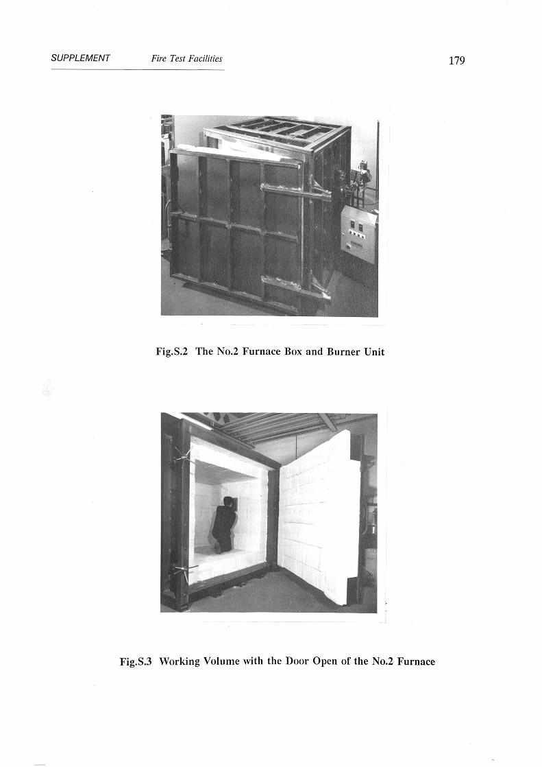
SUPPLEMENT Fire Test Facilities
Fig.S.2 The No.2 Furnace Box and Burner Unit
179
Fig.S.3 Working Volume with the Door Open of the No.2 Furnace

4
250
A-
1700
45
3005r FURNACE 3
SUPPLEMENT Fire Test Facilities 180
20001. FIRING SYSTEM
--I I-- 300 TROLLEY MOUNTED2. JET FLAME3. TEST PIPE4. TV CAMERA
5 5. FLUE PIPE8 CERAMIC FIBRE INSULATION
—4 250 250 --1 I--
Fig.S.4 Schematic Elevation of the No.2 Furnace
I. FIRING SYSTEM—TROLLEYMOUNTED
2. VERTICAL FLUE3. HINGED DOOR
. REMOVABLE ROOF PANELTV CAMERA—LOCATION FORVIEWING PANEL
8002000
A— —1— 2000 —
Fig.S.5 Schematic Plan of the No.2 Furnace

SUPPLEMENT Fire Test Facilities 181
enclosed environment. Firing was from the side using a powerful single 15 therm burner.
The flue exit was located just above the floor level, and measured 300mm x 300mm.
Figure S.4 is a schematic diagram of the furnace box arrangement and Figure S.5 shows
the laboratory layout which includes a separate control and viewing room. Figure S.6
shows an Ameron pipe with reinforced Pitt-Char within the furnace after an 8 minutes
hydrocarbon fire test.
Fig.S.6 Ameron Pipe Coated with Pitt-Char after Hydrocarbon Fire Test

SUPPLEMENT Fire Test Facilities 182
Haar's Experiment Arrangement
A schematic review of the test arrangement of Harr's experiments which were quoted in
Chapter 8 is given in Fig.S.7 [8.3]. For each test, six unloaded test deck slabs were laid
upon furnace using a temporary support in the centre of the fire compartment. The
gaps between the test specimens were sealed with strips of ceramic blanket (thickness
25mm).
The slabs were not protected by means of any insulation or suspended ceiling. To ensure
that the specimens would not fail during testing, additional reinforcement (08 and 06)
was included(Fig.S.8).
About 35 temperature measuring points were provided per specimen, spread over 3
sections: I, II and III (Fig.S.8). The thermocouples in sections I and III were used to
check the longitudinal symmetry of the thermal behaviour. The thermocouples in the
mid span section II were used to check the transverse symmetry of the thermal
behaviour. The thermocouples were positioned with care, a supporting frame being
applied to ensure that the thermocouples would not change position during pouring of
of the concrete. Nevertheless, small differences between these planned positions and
actual positions were observed after manufacturing of the specimens. The actual
positions were used in the numerical modelling in this thesis.

I1
.........-
1I
T—I ..„.. ---.1.-
--1i
0 11
n .1 1
11 I
11I11
1,.i„.._i1 .--;
1
......,—. , ,L-_-_
.......
-_- •
........
_ 1. :-
..--
_--.-.. ,.
---,, 1
4 __,I.
6 test specimen;
SUPPLEMENT Fire Test Facilities 183
0 wall of 'aerated concrete blocks in thecentre of the fire compartment.
0 concrete wall closing the fire compartment
0 concrete slabs on furnace walls
@ layer of 25 mm ceramic fibre banket atvertical concrete planes.
osition burner
300 250 2001350 1350
135 135
20-04,
1600 1600 *
(mm)
Fig.S.7 Schematic Review of the Harr's Test Arrangement [8.3]
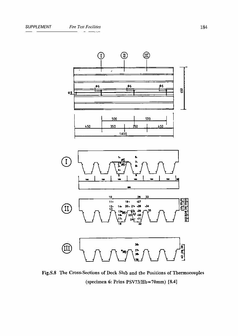
0 ® ©IMMn
.,
1 _06 L.106 1_106
4-1 00 .1
---
500
450 350
1600
500
450
10
2833
1 6
32
11. 19 • .27
12. 14. 20. 21 .26 .3413
15143.29le. 25 V .3017. 2 • •31
36
le4
ffn ng"' A
SUPPLEMENT Fire Test Facilities
104
tan
WI
NM
elli
184
Fig.S.8 The Cross-Sections of Deck Slab and the Positions of Thermocouples
(specimen 6: Prins PSV73/Hb=70mm) [8.4]