entropy

Article

Exergetic and Economic Evaluation of a TranscriticalHeat-Driven Compression Refrigeration System withCO2 as the Working Fluid under HotClimatic Conditions

Jing Luo 1,* , Tatiana Morosuk 1, George Tsatsaronis 1 and Bourhan Tashtoush 2

1 Institute for Energy Engineering, Technische Universität Berlin, Marchstr. 18, 10587 Berlin, Germany;tetyana.morozyuk@tu-berlin.de (T.M.); georgios.tsatsaronis@tu-berlin.de (G.T.)

2 Mechanical Engineering Department, Jordan University of Science and Technology, Ar Ramtha 3030, Jordan;bourhan@just.edu.jo

* Correspondence: jing.luo@campus.tu-berlin.de; Tel.: +49-(0)30-314-23280

Received: 2 November 2019; Accepted: 24 November 2019; Published: 28 November 2019 �����������������

Abstract: The purpose of this research is to evaluate a transcritical heat-driven compressionrefrigeration machine with CO2 as the working fluid from thermodynamic and economic viewpoints.Particular attention was paid to air-conditioning applications under hot climatic conditions.The system was simulated by Aspen HYSYS® (AspenTech, Bedford, MA, USA) and optimizedby automation based on a genetic algorithm for achieving the highest exergetic efficiency. In thecase of producing only refrigeration, the scenario with the ambient temperature of 35 ◦C and theevaporation temperature of 5 ◦C showed the best performance with 4.7% exergetic efficiency, while theexergetic efficiency can be improved to 22% by operating the system at the ambient temperatureof 45 ◦C and the evaporation temperature of 5 ◦C if the available heating capacity within the gascooler is utilized (cogeneration operation conditions). Besides, an economic analysis based on thetotal revenue requirement method was given in detail.

Keywords: transcritical heat-driven refrigeration machine; carbon dioxide; optimization; exergyanalysis; economic analysis

1. Introduction

Refrigeration systems with different configurations, thermodynamic cycles, and working fluidsare used for maintaining the temperature of an object below the ambient temperature. They are alsoconsidered as one of the essential parts of various industries/applications, e.g., food preservation,air conditioning, chemical industries, and biotechnologies. For the areas without a secure powersupply, heat-driven compression refrigeration machine is considered as one of the most promisingtechnologies since it has several unique advantages, for example, high efficiency, simple design, as wellas the opportunity of utilizing an inexpensive low-grade energy source.

The first heat-driven compression refrigeration machine was proposed by Chistiakov and Plotnikov(USSR) in the year of 1952 and reported in detail by Rosenfeld and Tkachev [1]. The idea was to “drive”a direct Organic Rankine Cycle (ORC) by the thermal energy, while the shaft work generated from theORC was further used to operate a vapor-compression refrigeration cycle (VCRC). Two subcycles werecombined by a mutual condenser. In terms of the working fluid, any of the working fluids—in general,either one-component or mixtures that are used for refrigeration cycles—could be applied [2,3], and thesame working fluid was used for both subcycles. During some period, the heat-driven compression

Entropy 2019, 21, 1164; doi:10.3390/e21121164 www.mdpi.com/journal/entropy

Entropy 2019, 21, 1164 2 of 18

refrigeration machines were out of the research interest. Recently, the interest in these machines hasbeen renewed.

Aphornratana and Sriveerakul [4] proposed a modified combined cycle of an ORC and a VCRC,which integrated the expander and compressor into a free-piston unit. R22 and R134a were examined asthe working fluids for the overall system. The results showed that the system achieved better coefficientof performance (COP) with R22. A prototype of an ORC–VCRC system with 5 kW refrigeration capacitywas tested in the laboratory and reported by Wang et al. [5]. R-245fa and R-134a were selected as theworking fluids for the power and the refrigeration sides, respectively. Since two different workingfluids were applied, two separate condensers in this experiment were used rather than a mutualcondenser, and the subcycles were only connected via the shaft work between the expander of thepower cycle and the compressor of the refrigeration cycle. The same research group also investigatedand compared three design configurations of the heat-driven refrigeration cycle [6]. The best cycle(with subcooling and cooling recuperation) showed a 22% improvement in terms of the COP to the basecase. In this research, the same working fluid (R-245fa) for both the power cycle and refrigeration cyclewas used. Thus, two subcycles were able to be combined through a mutual condenser. Bu et al. [7]focused on the discovery of the most suitable working fluid for an ORC–VCRC ice-maker driven bysolar energy. Four working fluids—R123, R-245fa, R-600a, and R600—were examined regarding theoverall energy efficiency. The results revealed that R123 had the best performance under the definedoperating conditions.

Four primary hydrocarbon working fluids were analyzed for an ORC–VCRC system for achievingbetter environmental performance (Li et al. [8]). With the assumption that the low-grade thermalenergy will be supplied, the conclusion was that R600 was the most promising working fluid withthe overall COP of 0.47. Similar research [9,10] was carried out to evaluate the performance offour working fluids with low Global Warming Potential (GWP) for a low-temperature heat-drivenORC–VCRC system. R-1336mzz(Z) and R-1233zd(E) were applied for the ORC, while R1234yf andR1234ze(E) were considered for the refrigeration cycle. The system performance for four differentcombinations of working fluids was thoroughly conducted. The results showed that the choice ofthe working fluid for the VCRC had only a slight effect on the overall system efficiency. In addition,the combination of R1336mzz(Z) for the power cycle and R1234ze(E) for the refrigeration cycleresulted in the highest energetic efficiency. Kim and Perez-Blanco [11] discussed a cogeneration system(producing power and refrigeration) by applying the heat-driven refrigeration machine. A limitingcase was mentioned as solely producing cold without net electricity by controlling the flow divisionratio. They concluded that the system exergetic efficiency was proportional to the refrigeration capacitywith a fixed source temperature and a given mass flow rate of the ORC. Nasir and Kim [12] investigatedseven working fluids with forty-nine combined options for an ORC–VCRC system driven by low-gradeheat. The ambient temperature was assumed between 30–40 ◦C, and the system was designed for airconditioning purposes with a room temperature of 15 ◦C. The best combination among the forty-nineoptions was R-134a and isobutane, with COP of 0.22.

In the publications mentioned above, one can conclude that selecting the suitable working fluid iscrucial for designing and operating the heat-driven ORC–VCRC systems. The selection of the workingfluid directly influences the thermodynamic performance of the system as well as the environmentalperformance. Besides, the safety, the reliability, and the cost of the working fluid should also be takeninto consideration. CO2 (R744) as a natural working fluid is getting more and more attention and hasbeen extensively researched since it is nontoxic, nonflammable, inexpensive, and environmentallybenign. For example, Lorentzen and Pettersen [13], as well as Cavallini and Zilio [14], discussed deeplyhow promising CO2 would be as a natural working fluid in the future. The low critical temperature(31.1 ◦C) and the high critical pressure (73.8 bar) of CO2 in conjunction with its thermodynamicproperties (slightly above critical point and near saturation lines) create a high potential for improvingthe thermodynamic and economic effectiveness of the refrigeration systems.

Entropy 2019, 21, 1164 3 of 18

However, the research of using CO2 as a refrigerant focused mainly on the transcritical VCRC. Forexample, Rozhentsev and Wang [15] discussed the thermodynamic efficiency of the heat regenerationwithin the transcritical VCRC, while Shiferaw at al. [16] evaluated the economic potential fortranscritical VCRC systems, and Fazelpour and Morosuk [17] proposed two optimal configurations ofthe transcritical VCRC with economizer from the exergoeconomic analysis point of view. The idea ofimplementing ejector technologies to a transcritical cascade refrigeration cycle was also reported [18,19].The information reported for the transcritical heat-driven refrigeration cycle considering CO2 as theworking fluid was minimal. In general, compared to conventional vapor-compression refrigerationmachines, it is advantageous to employ thermally-driven vapor compression refrigeration machines toensure the stable refrigeration capacity (for food and vaccine preservation, and/or for air conditioning)for the areas without a secure power supply. Besides, driving the vapor-compression refrigerationmachines by heat offers more system flexibility as it is possible to integrate the system into other systemsby utilizing any kinds of heat sources, and the system can produce not only refrigeration capacity butalso power and heating capacities based on the local requirements. Using CO2 as the working fluid fora heat-driven VCRC provides additional potentials for reducing the size of the system, for improvingthe system efficiency and for reducing the system cost as well. This is appealing for waste heat recoveryapplications to improve the system efficiency, for ship and automotive applications due to the limitedspace, and for offices, hotels, and other buildings where refrigeration, power, and heating capacitiesare needed simultaneously.

The performance of a waste heat-driven vapor compression refrigeration machine using CO2 asthe working fluid has been discussed by authors [20]. The system was designed to utilize the low-gradewaste heat, and four scenarios with various evaporation temperatures were evaluated and comparedfor storage of a wide range of food products and air conditioning applications. This work aimed topay special attention to air conditioning applications for countries or regions having hot climates(for example, the Middle East, India, and South China) since these countries/regions are developingsubstantially and with massive populations, which leads to considerable energy consumption for airconditioning purpose.

2. System Description

Figure 1 presents the schematic of a transcritical heat-driven compression refrigeration systemwith R744 inspired by Chistiakov and Plotnikov [1]. The system coupled a closed power cycle(Brayton cycle) with a transcritical refrigeration cycle. It consists of nine components: an evaporator(EVAP), a compressor for refrigeration cycle (CM_R), a mixer (MIX), a gas cooler (GC), a splitter(SPLIT), a throttling valve (TV), a compressor for power cycle (CM_P) as well as a heater (HE) and anexpander (EX).

The features of the new system are as follows:

• R744 is the only working fluid for both subsystems.• The power cycle operates entirely in the supercritical region, and part of the refrigeration cycle is

above the critical point.• The shafts of the expander and two compressors are directly connected.• The refrigeration capacity of the evaporator is the main product.• The net shaft work (can be further converted to electricity), which is the difference between the

power generation of the expander and the total power consumption of two compressors, can beproduced as the second product of the system.

• The available heating capacity within the gas cooler can be considered as the third productdepending on the local requirements.

• Any kinds of heat sources, in general, can be used for driving the system, for example, solar thermalenergy, geothermal heat, heat from biomass and waste heat from chemical plants and internalcombustion engines. The low-medium grade waste heat was focused in this study.

Entropy 2019, 21, 1164 4 of 18

Besides,

• the machine is used for air conditioning purposes (TEVAP = 5 and 15 ◦C [21]), and• hot climatic operation conditions were assumed (T0 = 35 and 45 ◦C [17]).

The following assumptions were made for the simulations:

• The refrigeration capacity is 100 kW.• The shaft work generated from the expander is merely sufficient to power both compressors,

.Wnet = 0 kW.

• The temperature of cooling water (stream 7) is equal to the assumed environmental temperature,T7 = T0.

• The temperature of “heat source” (HS) for the heater is always 20 K higher than the turbine inlettemperature (TIT): THS = TTIT + 20 K. Since the system in this work is considered to be driven bywaste heat (for example, waste heat from flue gases), a gas–gas heat exchanger is assumed.

• The outlet stream from the evaporator (stream 1) is saturated vapor (since it has been provedthat the effect of the superheating process within the evaporator for transcritical refrigerationmachines can be neglected [15]).

• The isentropic efficiency of both compressors, CM_P and CM_R (turbo-compressor), is equal to0.85 [21].

• The isentropic efficiency of the expander (turbo-expander) is assumed to be equal to 0.9 [21].• The gas cooler and the evaporator are considered to operate with the pinch temperature difference

of 5 K.• The simulation is completed under steady-state conditions. The pressure drops in pipes,

heat exchangers, as well as within the mixer and the splitter are neglected.

Entropy 2019, 21, x 4 of 19

• hot climatic operation conditions were assumed (T0 = 35 and 45 °C [17]). The following assumptions were made for the simulations:

• The refrigeration capacity is 100 kW. • The shaft work generated from the expander is merely sufficient to power both compressors, W = 0 kW. • The temperature of cooling water (stream 7) is equal to the assumed environmental temperature,

T7 = T0. • The temperature of “heat source” (HS) for the heater is always 20 K higher than the turbine inlet

temperature (TIT): THS = TTIT + 20 K. Since the system in this work is considered to be driven by waste heat (for example, waste heat from flue gases), a gas–gas heat exchanger is assumed.

• The outlet stream from the evaporator (stream 1) is saturated vapor (since it has been proved that the effect of the superheating process within the evaporator for transcritical refrigeration machines can be neglected [15]).

• The isentropic efficiency of both compressors, CM_P and CM_R (turbo-compressor), is equal to 0.85 [21].

• The isentropic efficiency of the expander (turbo-expander) is assumed to be equal to 0.9 [21]. • The gas cooler and the evaporator are considered to operate with the pinch temperature

difference of 5 K. • The simulation is completed under steady-state conditions. The pressure drops in pipes, heat

exchangers, as well as within the mixer and the splitter are neglected.

(a) (b)

Figure 1. (a) Schematic and (b) thermodynamic cycle of a transcritical heat-driven compression refrigeration machine with R744.

3. Methods

The simulations were carried out by Aspen HYSYS® Software (AspenTech, Bedford, MA, USA). Moreover, the exergy-based method was applied for optimizing, comparing, and investigating the system under various operation conditions. The Span–Wagner equation of state was selected for calculating the thermodynamic properties of CO2 since it is one of the most accurate models to predict CO2 behaviors in a wide range of temperature and pressure, including a high temperature, at high pressure and in the vicinity of its critical point [22]. To conduct the exergy-based method, the

Figure 1. (a) Schematic and (b) thermodynamic cycle of a transcritical heat-driven compressionrefrigeration machine with R744.

3. Methods

The simulations were carried out by Aspen HYSYS® Software (AspenTech, Bedford, MA, USA).Moreover, the exergy-based method was applied for optimizing, comparing, and investigating thesystem under various operation conditions. The Span–Wagner equation of state was selected forcalculating the thermodynamic properties of CO2 since it is one of the most accurate models to predict

Entropy 2019, 21, 1164 5 of 18

CO2 behaviors in a wide range of temperature and pressure, including a high temperature, at highpressure and in the vicinity of its critical point [22]. To conduct the exergy-based method, the referencetemperature T0 varies when the assumption of the ambient temperature varies (T0 = 35/45 ◦C), while thereference pressure p0 in this study keeps constant (p0 = 1.013 bar).

3.1. Optimization

The system optimization was first carried out for achieving the highest exergetic efficiency of thesystem operating under different conditions. Aspen HYSYS was connected with the programminglanguage, Python, through a binary-interface, component object model (COM), which allows thecommunication between these two programs. A genetic algorithm (GA) as a metaheuristic optimizationtechnique was selected to conduct the optimization. The algorithm is inspired by Charles Darwin’stheory, which describes the process of natural evolution to solve complex optimization problems.The fittest individual will be finally generated and selected after several generations through selection,crossover, and mutation procedures [23]. In this study, the objective function was defined to maximizethe exergetic efficiency of the overall system. The population size was set at 100, the uniform crossoverwas applied, and the mutation rate was tuned as 0.3. The optimization procedure terminates after teniterations, and the constraints of the design variables are listed in Table 1.

Table 1. Ranges of design variables. (PRc: pressure ratio within the compressors.).

Design Variable Range

T10 (◦C) 220–500 [24,25]p10 (bar) 150–200 [21,26,27]

PRc 1.7–3.0T3 (◦C) ≥32 [25,28]p3 (bar) ≥77 [25,28]

The expander inlet operation conditions are T10 and p10. The pressure ratio within the compressorsis PRc. The outlet stream of R744 from the GC is with T3 and p3. The maximum pressure for operatingthe supercritical CO2 power cycle is assumed to be 200 bar [21,26,27] because higher operating pressurewill lead to thicker walls and more expensive materials, which increases the cost of the overall system.

3.2. Analysis

The comparison of the system with different ambient temperatures and evaporation temperatureswas then implemented from energetic, exergetic, and economic viewpoints. The equations of energeticand exergetic evaluations were given from different perspectives by considering the system as therefrigeration system, cogeneration system, and trigeneration system.

3.2.1. Energetic Analysis

The energetic efficiency of the overall system can be defined as follows:• for trigeneration (heat, refrigeration, and power):

COPOverall =( .QGC +

.Wnet

)/

.QHE, (1)

• for cogeneration (refrigeration and heat):

COPOverall =.

QGC/.

QHE, (2)

• for cogeneration (refrigeration and power):

COPOverall =( .QEVAP +

.Wnet

)/

.QHE, (3)

Entropy 2019, 21, 1164 6 of 18

• for only refrigeration:COPOverall =

.QEVAP/

.QHE. (4)

While, for two subsystems, the expressions of the energetic efficiency are as follows:The closed power cycle, ηP

• for trigeneration (heat, refrigeration, and power) or cogeneration (refrigeration and heat):

ηP =( .WEX −

.WCM_P +

.QGC,P

)/

.QHE, (5)

• for cogeneration (refrigeration and power) or only refrigeration:

ηP =( .WEX −

.WCM_P

)/

.QHE, (6)

the refrigeration cycle, COP• for trigeneration (heat, refrigeration, and power) or cogeneration (refrigeration and heat):

COP =.

QGC,R/.

WCM_R, (7)

• for cogeneration (refrigeration and power) or only refrigeration:

COP =.

QEVAP/.

WCM_R. (8)

Here,.

QEVAP is the desired refrigeration capacity,.

Wnet is the net power output,.

QGC is the availableheating capacity, and

.QHE is the heat absorbed from the heat sources.

.QGC,P and

.QGC,R are the heat

capacities contributed by the power cycle and the refrigeration cycle, respectively, if the system istreated as two subsystems.

The.

Wnet is expressed as.

Wnet =.

WEX −.

WCM_P −.

WCM_R. (9).

QGC,P and.

QGC,R are proportional to the mass flow rate ratios of the power cycle mass flow rateand refrigeration cycle mass flow rate to the overall mass flow rate, respectively. Additionally, the sumof

.QGC,P and

.QGC,R should equal to the total heat capacity within the GC,

.QGC:

.QGC,P =

.mP( .

mP +.

mR) ∗ .

QGC, (10)

.QGC,R =

.mR( .

mP +.

mR) ∗ .

QGC, (11)

.QGC,P +

.QGC,R =

.QGC. (12)

3.2.2. Exergetic Analysis

In addition to energy analysis, the exergetic evaluation was conducted based on the exergy offuel/exergy of product approach (for the kth component and the overall system) to identify the locationand the magnitude of the irreversibilities [29]. The exergetic efficiency ε is expressed as the ration ofexergy of product (

.EP) and exergy of fuel (

.EF):

ε =.EP/

.EF. (13)

Neglecting the variations of the potential exergy, the kinetic exergy, as well as the chemical exergy,only physical exergy was considered in this work. However, the physical exergy of the material stream

Entropy 2019, 21, 1164 7 of 18

needs to be split into the thermal (.E

T) and mechanical (

.E

M) parts since several components operate

below and cross the ambient temperature [30]:

.E

PH=

.E

T+

.E

M. (14)

For the kth component, the value difference between the exergy of fuel and the exergy of theproduct is the exergy destruction, which indicates the irreversibilities within the component:

.EF,k −

.EP,k =

.ED,k, (15)

while, for the overall system, the difference between the fuel and the product is not only the exergydestruction but also the exergy loss (

.EL,tot), which is defined as the exergy transferred into the

environment [29]:.EF,tot −

.EP,tot =

.ED,tot +

.EL,tot. (16)

The definitions of the fuel, the product, the destruction, and the loss for each component, as wellas for the overall system, are given in Table 2. The fuel and the product for the mixer were not definedsince the mixer was considered as a dissipative component [29]. Moreover, for the overall system,various product definitions are given regarding the total number of products that have been considered.

Table 2. Exergy of fuel, product, and losses for each component and the overall system.

Component/System Exergy of Fuel (.EF) Exergy of Product (

.EP) Exergy of Loss (

.EL)

Evaporator (EVAP).E4 −

.E1

.E6 −

.E5 -

Compressor for refrigeration cycle (CM_R).

WCM_R +.E

T1

.E

T2_1 +

.E

M2_1 −

.E

M1 -

Mixer (MIX) - - -Gas cooler (GC)

.E2 −

.E3

.E8 −

.E7 -

Throttling valve (TV).E

M3_1 −

.E

M4 +

.E

T3_1

.E

T4 -

Compressor for power cycle (CM_P).

WCM_P.E9 −

.E3_2 -

Heater (HE).

QHE

(1− T0

THS

) .E10 −

.E9 -

Expander (EX).E10 −

.E2_2

.WEX -

Overall (only refrigeration).

QHE

(1− T0

THS

) .E6 −

.E5

.E8 −

.E7

Overall (refrigeration and heat).

QHE

(1− T0

THS

) .E6 −

.E5 +

.E8 −

.E7 0

Overall (refrigeration and power).

QHE

(1− T0

THS

) .E6 −

.E5 +

.Wnet

.E8 −

.E7

Overall (heat, refrigeration, and power).

QHE

(1− T0

THS

) .E6 −

.E5 +

.Wnet+

.E8 −

.E7 0

3.2.3. Economic Analysis

To analyze the system from an economic viewpoint, the total revenue requirement (TRR) methodwas applied [29]. For conducting the TRR, the total capital investment (TCI) of the system was firstestimated based on the purchased equipment cost (PEC) of each component, then the economic,financial, operating, and market input parameters were determined for the detailed cost calculation.Finally, the geometrically increasing series of expenditures will be levelized into a financially equivalentconstant quantity (annuity). The final equation for calculating the levelized total revenue requirementis written as

TRRL = CCL + FCL + OMCL, (17)

where CCL stands for levelized carrying charges, FCL is the levelized fuel cost, and OMCL is forlevelized operating and maintenance costs.

In addition, the CCL is calculated as

CCL = TCI ∗CRF, (18)

Entropy 2019, 21, 1164 8 of 18

where CRF is the capital recovery factor and can be given by

CRF =ie f f(1 + ie f f

)n(1 + ie f f

)n− 1

, (19)

ie f f and n are the effective interest rate and the economic lifetime of the power plant, respectively.FCL is determined by the fuel cost at the beginning of the first year FC0 and the constant escalation

levelization factor (CELF):

FCL = FC0 ∗CELF = FC0 ∗kFC(1− kn

FC

)1− kFC

∗CRF, (20)

withkFC =

1 + rFC1 + ie f f

. (21)

The same procedure was applied for OMCL:

OMCL = OMC0 ∗CELF = OMC0 ∗kOMC

(1− kn

OMC

)1− kOMC

∗CRF, (22)

withkOMC =

1 + rOMC1 + ie f f

, (23)

where rFC and rOMC stand for the average inflation rate of the fuel cost and the operating andmaintenance cost, respectively.

All the assumptions made for the economic analysis are summarized in Table 3. The fuel cost wasassumed to be free of charge since the heat source is unknown.

Table 3. Assumptions for economic analysis.

Variable Nomenclature Unit Value

The economic lifetime of the power plant n a 20Annual full load hours τ h a−1 8000Effective interest rate ieff % 10

Average general inflation rate rFC, rOMC % 2.5Total Capital Investment TCI $ 6.32 PEC [29]

Fuel cost at the beginning of the first year FC0 $ 0Operating and maintenance cost at the

beginning of the first year OMC0 $ 0.05 TCI n−1

The key and the most challenging part of an economic evaluation is to estimate the PEC of eachcomponent, especially for the new and uncommercialized technology. Therefore, in the followingsections, the procedures applied for estimating the PEC for all the components of the system areexplained in detail.

• HE and GC

Since the HE and GC were expected to work at high-temperature and high-pressure, the printedcircuit heat exchanger (PCHE) technology was selected to fulfill the requirements of the closed powercycle rather than a standard shell and tube heat exchanger [16,31]. The PCHE technology is a relativelynew technology applied for manufacturing compact heat exchangers by photoetching microchanneltechnology and a specific solid-state joining process to boost the mechanical integrity and efficiency,technology readiness level, and flexibility of heat exchangers [14,25]. Meanwhile, the capital cost

Entropy 2019, 21, 1164 9 of 18

of the overall system was expected to be reduced by replacing the shell and tube heat exchangersby the PCHE. Based on the research of “Heatric” (UK) [32] that has already started to producePCHEs for supercritical cycle applications, the cost of a PCHE should be estimated by its weight:CostPCHE = Cost per unit massmetal ∗MassPCHE, with MassPCHE = Densitymetal ∗Volumemetal. To calculatethe volume of the metal that was used for manufacturing the heat exchanger, the volume fraction ofthe metal to the heat exchanger per m3, fm was needed, Volumemetal = VolumePCHE ∗ fm. The size of theheat exchanger VolumePCHE can be estimated by the area of the heat exchanger and the information ofthe typical area per unit volume, VolumePCHE =

APCHEtypical area per unit volume . Depending on the operating

pressure, the typical area per unit volume for PCHEs is around 1300 m2/m3 at 100 bar and 650 m2/m3

at 500 bar [32]. The heat-transfer area of the heat exchanger APCHE, was calculated by the equation Q =

U A TLMTD. Q stands for the transferred heat within the heat exchanger; U is the overall heat-transfercoefficient; and TLMTD is the log mean temperature difference. The assumptions made for estimatingthe cost of PCHEs are summarized in Table 4.

Table 4. Assumptions for the cost estimation of printed circuit heat exchangers (PCHEs).

Item Nomenclature Value Unit

Overall heat-transfer coefficient U 500 [32] W m−2K−1

The fraction of metal per m3 of the heat exchanger fm 0.564 [27] m3 m−3

The density of stainless steel DensitySS 7800 kg m−3

Cost of stainless steel per unit mass Cost per unit massSS 50 [32] $ kg−1

• Turbomachinery (CM_P and EX)

Since the turbomachinery operating with R744 is not well known for commercial application yet,the costs of the expander and compressor in the closed power cycle were scaled from the available costinformation for helium turbomachinery [27]:

Temperature Proportionality Constant = 3.35 +( TIT

1000

)7.8, (24)

Pressure Proportionality Constant = TIP−0.3, (25)

Power Capacity Proportionality Constant = P285

TIP1.7 + 0.6

G , (26)

where TIT is the expander inlet temperature in ◦C, TIP is the expander inlet pressure in bar, and thePG represents the power generated within expander in MW.

• CM_R and EVAP

For the compressor and the evaporator of the transcritical refrigeration cycle, their costs wereconsidered as a function of the capacity. Furthermore, the cost correction factors were also consideredregarding materials, design pressure, and design temperature [33]: CE = CB ∗ (X/XB)

M fM fP fT,where CE is the new equipment cost with capacity X, CB is the known base cost for equipment withcapacity XB, M is an exponent, and fM, fP and fT are the correction factors in terms of materials,design pressure, and design temperature, respectively.

Moreover, the power consumption was used as the capacity X for estimating the cost of thecompressor, while, for the evaporator, X refers to the heat-transfer area of the heat exchanger.For calculating the heat-transfer area of the evaporator, the overall heat-transfer coefficient was set to950 W/(m2K) [17]. In Table 5, the values used for the cost estimation of the compressor and evaporatorare listed.

Entropy 2019, 21, 1164 10 of 18

Table 5. The values used for computing the costs of the compressor for refrigeration cycle (CM_R) andevaporator (EVAP) [33].

CM_R

CB ($) XB (kW) M fM fP fT98,400 250 0.95 [29] 1 1.5 1

EVAP

CB ($) XB (m2) M fM fP fT32,800 80 0.68 1 1.3 1

• Other components

For the PECs of the TV and others, the following assumptions were made:

1. For the refrigeration machine with the cooling capacity of 100 kW, the cost of the TV equals to100 € [17];

2. The costs of the mixer and the splitter are neglected.

Finally, the costs of all components were brought up-to-date using the cost indices [33] fromChemical Engineering (CE) and applied in US$2017:

Cost at the re f erence year = Original cost ×Cost index f or the re f erence year

Cost index f or the original year cost. (27)

4. Results and Discussion

4.1. Thermodynamic Investigations

In this study, the performance of a transcritical heat-driven refrigeration system with R744 asthe working fluid for both subsystems was investigated. Four scenarios focusing on air conditioningapplications (TEVAP = 5 and 15 ◦C) under hot climatic conditions (T0 = 35 and 45 ◦C) were simulated,optimized, and compared. Table 6 demonstrates the exergetic optimization results aiming at thehighest exegetic efficiency of the overall system for each scenario.

Table 6. Exergetic optimization results for each operation scenario.

T0 = 35 ◦C T0 = 45 ◦CTEVAP = 5 ◦C TEVAP = 15 ◦C TEVAP = 5 ◦C TEVAP = 15 ◦C

Operating parameters

T10 (◦C) 220 220 220 220p10 (bar) 200 200 200 200T3 (◦C) 50 50 40 40p3 (bar) 95 95 112 112PRP (-) 2.11 2.11 1.79 1.79PRR (-) 2.48 1.92 2.91 2.27

mP(kg h−1) 4558.22 3267.43 10,289.66 8080.17mR (kg h−1) 3396.58 3776.06 4535.40 5138.80mP/mR (-) 1.34 0.87 2.27 1.57

Energetic results

ηP (%) 10.92 10.92 8.56 8.56COP (-) 2.56 3.57 1.59 2.03

COPoverall (-) 0.28 0.39 0.14 0.17

Exergetic results

εP (%) 27.35 27.35 22.52 22.52εR (%) 17.07 11.14 16.10 13.14

εOverall (%) 4.67 3.05 3.63 2.93.EHeating/

.ECooling (-) 2.73 3.95 5.08 5.90

Entropy 2019, 21, 1164 11 of 18

The results showed that the lowest T10 but the highest p10 were selected for each scenario, while theoptimal T3 and p3 depended on the ambient temperature rather than the evaporation temperature.Hence, the closed power cycle, for various scenarios with the same ambient temperature, was suggestedto operate at the same conditions. Only the

.mP differed, but the energetic and exergetic efficiencies of

the power cycle with the same ambient conditions were consistent. Meanwhile, for the transcriticalrefrigeration cycle, by changing the evaporation temperature from 5 to 15 ◦C, the pressure ratio PRR andthe

.mP varied simultaneously, which affected its energetic and exergetic efficiencies. With the higher

evaporation temperature, the higher COP of the transcritical refrigeration cycle was achieved as well asthe better energy performance of the overall system. While the exergetic efficiencies of the refrigerationcycle and the overall system decreased significantly by increasing the evaporation temperature.

By increasing the ambient temperature, the energetic and the exergetic efficiencies of bothsubsystems dropped, which resulted in lower performance of the overall system. One can concludethat the system operating with the evaporation temperature of 15 ◦C (higher evaporation temperature)and the ambient temperature of 35 ◦C (lower ambient temperature) yielded the best energetic efficiencyof 0.39; while the highest exergetic efficiency (4.67%) of the overall system was achieved with lowerevaporation temperature (5 ◦C) and lower ambient temperature (35 ◦C). In addition, the ratio of theavailable heating product to the refrigeration product in terms of exergy (

.EHeating/

.ECooling) was notable,

particularly at higher ambient temperature. Hence, the overall exergetic efficiencies of the scenarioswith and without utilizing the available heat capacity were investigated in Figure 2.

Entropy 2019, 21, x 11 of 19

Energetic results 𝜂 (%) 10.92 10.92 8.56 8.56 COP (-) 2.56 3.57 1.59 2.03 𝐶𝑂𝑃 (-) 0.28 0.39 0.14 0.17

Exergetic results 𝜀 (%) 27.35 27.35 22.52 22.52 𝜀 (%) 17.07 11.14 16.10 13.14 𝜀 (%) 4.67 3.05 3.63 2.93 𝐸 /𝐸 (-) 2.73 3.95 5.08 5.90

By increasing the ambient temperature, the energetic and the exergetic efficiencies of both subsystems dropped, which resulted in lower performance of the overall system. One can conclude that the system operating with the evaporation temperature of 15 °C (higher evaporation temperature) and the ambient temperature of 35 °C (lower ambient temperature) yielded the best energetic efficiency of 0.39; while the highest exergetic efficiency (4.67%) of the overall system was achieved with lower evaporation temperature (5 °C) and lower ambient temperature (35 °C). In addition, the ratio of the available heating product to the refrigeration product in terms of exergy ( 𝐸 /𝐸 ) was notable, particularly at higher ambient temperature. Hence, the overall exergetic efficiencies of the scenarios with and without utilizing the available heat capacity were investigated in Figure 2.

(a)

4.67

3.05

17.40

15.09

0.00

5.00

10.00

15.00

20.00

5 15

Exer

getic

effi

cien

cy (%

)

Evaporation temperature (°C)

Cooling Cooling and HeatingT0 = 35 °C

Entropy 2019, 21, x 12 of 19

(b)

Figure 2. 𝜀 with and without available heating product for different environmental temperatures by varying evaporation temperatures (a) T0 = 35 °C and (b) T0 = 45 °C.

The following conclusions can be made:

• For different ambient operating conditions (ambient temperatures of 35 and 45 °C), the exergetic efficiency of the overall system (with and without available heating product) decreased with increasing the evaporation temperature. Therefore, the system was preferred to operate at a lower evaporation temperature.

• By varying the ambient temperature from 35 to 45 °C, the exergetic efficiency with the consideration of utilizing only refrigeration products reduced, while the efficiency was improved once the heating product was also taken into consideration. It revealed that the ambient temperature had a significant effect on the amount of the available heating capacity, and a large amount of heat, particularly at higher ambient temperature, should be utilized based on the local requirements to improve the performance of the overall system.

The products of the system in exergy for each scenario were summarized in Figure 3. Since net power generation was assumed as 0 kW in this study, the products were only considered regarding refrigeration and heat capacities. Around 10 kW of refrigeration capacity and more than 50 kW heat capacity can be produced by the system with the ambient temperature of 45 °C and the evaporation temperature of 5 °C. However, by operating the system at the ambient temperature of 35 °C and the evaporation temperature of 15 °C, only 3.12 kW and 12.35 kW as refrigeration and heat capacities, respectively, were available.

Figure 4 demonstrates the exergetic efficiency of each component for four scenarios. The results showed that the expander and two compressors had the best performance (with exergetic efficiency more than 85%). The heat exchangers (EVAP, GC, and HE) had relatively low efficiency, which was between 45–70%, while the TV had the lowest efficiency (lower than 45%), which needed to be further considered in order to improve the overall system performance (for example, as it was discussed in [17]). In addition, the variations of exergetic efficiencies within the EVAP, the GC, and the TV were quite notable, since their operating conditions changed considerably by adjusting the evaporation and ambient temperatures.

3.63 2.93

22.0420.21

0.00

5.00

10.00

15.00

20.00

25.00

5 15

Exer

getic

effi

cien

cy (%

)

Evaporation temperature ( °C)

Cooling Cooling and HeatingT0 = 45 °C

Figure 2. εOverall with and without available heating product for different environmental temperaturesby varying evaporation temperatures (a) T0 = 35 ◦C and (b) T0 = 45 ◦C.

Entropy 2019, 21, 1164 12 of 18

The following conclusions can be made:

• For different ambient operating conditions (ambient temperatures of 35 and 45 ◦C), the exergeticefficiency of the overall system (with and without available heating product) decreased withincreasing the evaporation temperature. Therefore, the system was preferred to operate at a lowerevaporation temperature.

• By varying the ambient temperature from 35 to 45 ◦C, the exergetic efficiency with the considerationof utilizing only refrigeration products reduced, while the efficiency was improved once theheating product was also taken into consideration. It revealed that the ambient temperature hada significant effect on the amount of the available heating capacity, and a large amount of heat,particularly at higher ambient temperature, should be utilized based on the local requirements toimprove the performance of the overall system.

The products of the system in exergy for each scenario were summarized in Figure 3. Since netpower generation was assumed as 0 kW in this study, the products were only considered regardingrefrigeration and heat capacities. Around 10 kW of refrigeration capacity and more than 50 kW heatcapacity can be produced by the system with the ambient temperature of 45 ◦C and the evaporationtemperature of 5 ◦C. However, by operating the system at the ambient temperature of 35 ◦C and theevaporation temperature of 15 ◦C, only 3.12 kW and 12.35 kW as refrigeration and heat capacities,respectively, were available.

Entropy 2019, 21, x 13 of 19

Figure 3. Cooling and heating products in exergy for each scenario (No net power generation).

Figure 4. Exergetic efficiency of components for each scenario.

Figure 5 illustrated the exergy balance of the overall system for each scenario. The part of the exergy associating with components was the exergy destruction within the corresponding component, and the potential product referred to exergy of the overall product (the refrigeration and heat capacities) that can be produced. The sum of the exergy destructions within the components and the potential product of the overall system was the exergy of fuel for the system. It can be noticed that the HE contributed the most to the exergy destruction (more than 40%) since the temperature difference within this component was set as 20 K, which was quite high for the refrigeration application. In addition, the values of the exergy destruction within the GC and the TV were considerable for each scenario. The reason for the high exergy destruction within the GC was due to the high-temperature difference and the high mass flow rate by combining two subsystems.

T_0 = 35 °C,T_EVAP = 5 °C

T_0 = 35 °C,T_EVAP = 15 °C

T_0 = 45 °C,T_EVAP = 5 °C

T_0 = 45 °C,T_EVAP = 15 °C

Heating 18.21 12.35 51.49 38.19Cooling 6.68 3.12 10.14 6.47

0.00

10.00

20.00

30.00

40.00

50.00

60.00

70.00

Prod

uct i

n ex

ergy

(kW

)

EVAP CM_R GC TV CM_P HE EXT_0=35 °C, T_EVAP=5 °C 61.92 87.55 45.41 46.28 86.46 58.91 92.47T_0=35 °C, T_EVAP=15 °C 44.99 87.07 47.08 42.71 86.46 58.91 92.47T_0=45 °C, T_EVAP=5 °C 70.52 87.93 58.28 39.95 86.39 58.73 92.49T_0=45 °C, T_EVAP=15 °C 62.14 87.56 59.12 37.84 86.37 58.51 92.50

30.00

40.00

50.00

60.00

70.00

80.00

90.00

100.00

Exer

getic

effi

cienc

y (%

)

Figure 3. Cooling and heating products in exergy for each scenario (No net power generation).

Figure 4 demonstrates the exergetic efficiency of each component for four scenarios. The resultsshowed that the expander and two compressors had the best performance (with exergetic efficiencymore than 85%). The heat exchangers (EVAP, GC, and HE) had relatively low efficiency, which wasbetween 45%–70%, while the TV had the lowest efficiency (lower than 45%), which needed to be furtherconsidered in order to improve the overall system performance (for example, as it was discussedin [17]). In addition, the variations of exergetic efficiencies within the EVAP, the GC, and the TV werequite notable, since their operating conditions changed considerably by adjusting the evaporation andambient temperatures.

Entropy 2019, 21, 1164 13 of 18

Entropy 2019, 21, x 13 of 19

Figure 3. Cooling and heating products in exergy for each scenario (No net power generation).

Figure 4. Exergetic efficiency of components for each scenario.

Figure 5 illustrated the exergy balance of the overall system for each scenario. The part of the exergy associating with components was the exergy destruction within the corresponding component, and the potential product referred to exergy of the overall product (the refrigeration and heat capacities) that can be produced. The sum of the exergy destructions within the components and the potential product of the overall system was the exergy of fuel for the system. It can be noticed that the HE contributed the most to the exergy destruction (more than 40%) since the temperature difference within this component was set as 20 K, which was quite high for the refrigeration application. In addition, the values of the exergy destruction within the GC and the TV were considerable for each scenario. The reason for the high exergy destruction within the GC was due to the high-temperature difference and the high mass flow rate by combining two subsystems.

T_0 = 35 °C,T_EVAP = 5 °C

T_0 = 35 °C,T_EVAP = 15 °C

T_0 = 45 °C,T_EVAP = 5 °C

T_0 = 45 °C,T_EVAP = 15 °C

Heating 18.21 12.35 51.49 38.19Cooling 6.68 3.12 10.14 6.47

0.00

10.00

20.00

30.00

40.00

50.00

60.00

70.00

Prod

uct i

n ex

ergy

(kW

)

EVAP CM_R GC TV CM_P HE EXT_0=35 °C, T_EVAP=5 °C 61.92 87.55 45.41 46.28 86.46 58.91 92.47T_0=35 °C, T_EVAP=15 °C 44.99 87.07 47.08 42.71 86.46 58.91 92.47T_0=45 °C, T_EVAP=5 °C 70.52 87.93 58.28 39.95 86.39 58.73 92.49T_0=45 °C, T_EVAP=15 °C 62.14 87.56 59.12 37.84 86.37 58.51 92.50

30.00

40.00

50.00

60.00

70.00

80.00

90.00

100.00

Exer

getic

effi

cienc

y (%

)

Figure 4. Exergetic efficiency of components for each scenario.

Figure 5 illustrated the exergy balance of the overall system for each scenario. The part of theexergy associating with components was the exergy destruction within the corresponding component,and the potential product referred to exergy of the overall product (the refrigeration and heat capacities)that can be produced. The sum of the exergy destructions within the components and the potentialproduct of the overall system was the exergy of fuel for the system. It can be noticed that the HEcontributed the most to the exergy destruction (more than 40%) since the temperature difference withinthis component was set as 20 K, which was quite high for the refrigeration application. In addition,the values of the exergy destruction within the GC and the TV were considerable for each scenario.The reason for the high exergy destruction within the GC was due to the high-temperature differenceand the high mass flow rate by combining two subsystems. Moreover, the high exergy destructionwithin the TV can be reduced only by modifying the configurations of the system.

Entropy 2019, 21, x 14 of 19

Moreover, the high exergy destruction within the TV can be reduced only by modifying the configurations of the system.

Figure 5. System exergy balance (exergy destruction of each component and potential product of the overall system in exergy) for each scenario.

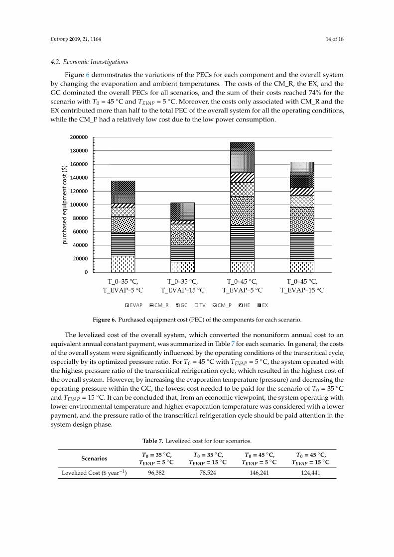
4.2. Economic Investigations

Figure 6 demonstrates the variations of the PECs for each component and the overall system by changing the evaporation and ambient temperatures. The costs of the CM_R, the EX, and the GC dominated the overall PECs for all scenarios, and the sum of their costs reached 74% for the scenario with T0 = 45 °C and TEVAP = 5 °C. Moreover, the costs only associated with CM_R and the EX contributed more than half to the total PEC of the overall system for all the operating conditions, while the CM_P had a relatively low cost due to the low power consumption.

The levelized cost of the overall system, which converted the nonuniform annual cost to an equivalent annual constant payment, was summarized in Table 7 for each scenario. In general, the costs of the overall system were significantly influenced by the operating conditions of the transcritical cycle, especially by its optimized pressure ratio. For T0 = 45 °C with TEVAP = 5 °C, the system operated with the highest pressure ratio of the transcritical refrigeration cycle, which resulted in the highest cost of the overall system. However, by increasing the evaporation temperature (pressure) and decreasing the operating pressure within the GC, the lowest cost needed to be paid for the scenario of T0 = 35 °C and TEVAP = 15 °C. It can be concluded that, from an economic viewpoint, the system operating with lower environmental temperature and higher evaporation temperature was considered with a lower payment, and the pressure ratio of the transcritical refrigeration cycle should be paid attention in the system design phase.

0.00

50.00

100.00

150.00

200.00

250.00

300.00

T_0=35 °C,T_EVAP=5 °C

T_0=35 °C,T_EVAP=15 °C

T_0=45 °C,T_EVAP=5 °C

T_0=45 °C,T_EVAP=15 °CEx

ergy

des

truc

tion

and

exer

gy p

rodu

ct(k

W)

EVAP CM_R MIX GC TV CM_P HE EX Potential product

Figure 5. System exergy balance (exergy destruction of each component and potential product of theoverall system in exergy) for each scenario.

Entropy 2019, 21, 1164 14 of 18

4.2. Economic Investigations

Figure 6 demonstrates the variations of the PECs for each component and the overall systemby changing the evaporation and ambient temperatures. The costs of the CM_R, the EX, and theGC dominated the overall PECs for all scenarios, and the sum of their costs reached 74% for thescenario with T0 = 45 ◦C and TEVAP = 5 ◦C. Moreover, the costs only associated with CM_R and theEX contributed more than half to the total PEC of the overall system for all the operating conditions,while the CM_P had a relatively low cost due to the low power consumption.

Entropy 2019, 21, x 15 of 19

Figure 6. Purchased equipment cost (PEC) of the components for each scenario.

Table 7. Levelized cost for four scenarios.

Scenarios T0 = 35 °C, TEVAP = 5 °C

T0 = 35 °C, TEVAP = 15 °C

T0 = 45 °C, TEVAP = 5 °C

T0 = 45 °C, TEVAP = 15 °C

Levelized Cost ($ year-1) 96,382 78,524 146,241 124,441

5. Conclusions

In this paper, a stand-alone transcritical heat-driven compression refrigeration system using CO2 as the working fluid was proposed. Compared to other vapor-compression refrigeration systems, the system, in general, can utilize any kinds of heat sources to produce refrigeration, heating, and power capacities simultaneously. This technology is beneficial to stabilize the refrigeration capacity for the areas without a secure power supply. Moreover, the system using CO2—a natural working fluid—as the refrigerant can be driven by renewable energies (for example, solar, geothermal, and biomass energies) and low to medium grade waste heat (for example, waste heat from chemical plants and internal combustion engines), which makes the system attractive from an environmental viewpoint. The low critical temperature (31.1 °C) and the high critical pressure (73.8 bar) of CO2 in conjunction with its thermodynamic properties (slightly above critical point and near saturation lines) create a high potential for improving the thermodynamic and economic effectiveness of the refrigeration systems.

In this work, the system for air conditioning purpose was thermodynamically and economically investigated. Special attention was given to countries and regions having hot climates and developing substantially. The refrigeration capacity of the system was assumed as 100 kW, and there was no net power generation. Four scenarios focusing on the air conditioning temperatures under hot climatic conditions were simulated and then optimized, aiming at the highest exergetic efficiency. The optimization results revealed that the five design variables were more sensitive to the ambient temperature rather than the evaporation temperature. With increasing the evaporation temperature, the exergetic efficiency of the overall system decreased. The system performed better, in general, under lower environmental conditions if the refrigeration capacity was considered as the sole

0

20000

40000

60000

80000

100000

120000

140000

160000

180000

200000

T_0=35 °C,T_EVAP=5 °C

T_0=35 °C,T_EVAP=15 °C

T_0=45 °C,T_EVAP=5 °C

T_0=45 °C,T_EVAP=15 °C

purc

hase

d eq

uipm

ent c

ost (

$)

EVAP CM_R GC TV CM_P HE EX

Figure 6. Purchased equipment cost (PEC) of the components for each scenario.

The levelized cost of the overall system, which converted the nonuniform annual cost to anequivalent annual constant payment, was summarized in Table 7 for each scenario. In general, the costsof the overall system were significantly influenced by the operating conditions of the transcritical cycle,especially by its optimized pressure ratio. For T0 = 45 ◦C with TEVAP = 5 ◦C, the system operated withthe highest pressure ratio of the transcritical refrigeration cycle, which resulted in the highest cost ofthe overall system. However, by increasing the evaporation temperature (pressure) and decreasing theoperating pressure within the GC, the lowest cost needed to be paid for the scenario of T0 = 35 ◦Cand TEVAP = 15 ◦C. It can be concluded that, from an economic viewpoint, the system operating withlower environmental temperature and higher evaporation temperature was considered with a lowerpayment, and the pressure ratio of the transcritical refrigeration cycle should be paid attention in thesystem design phase.

Table 7. Levelized cost for four scenarios.

Scenarios T0 = 35 ◦C,TEVAP = 5 ◦C

T0 = 35 ◦C,TEVAP = 15 ◦C

T0 = 45 ◦C,TEVAP = 5 ◦C

T0 = 45 ◦C,TEVAP = 15 ◦C

Levelized Cost ($ year−1) 96,382 78,524 146,241 124,441

Entropy 2019, 21, 1164 15 of 18

5. Conclusions

In this paper, a stand-alone transcritical heat-driven compression refrigeration system using CO2

as the working fluid was proposed. Compared to other vapor-compression refrigeration systems,the system, in general, can utilize any kinds of heat sources to produce refrigeration, heating, and powercapacities simultaneously. This technology is beneficial to stabilize the refrigeration capacity for theareas without a secure power supply. Moreover, the system using CO2—a natural working fluid—asthe refrigerant can be driven by renewable energies (for example, solar, geothermal, and biomassenergies) and low to medium grade waste heat (for example, waste heat from chemical plants andinternal combustion engines), which makes the system attractive from an environmental viewpoint.The low critical temperature (31.1 ◦C) and the high critical pressure (73.8 bar) of CO2 in conjunctionwith its thermodynamic properties (slightly above critical point and near saturation lines) create a highpotential for improving the thermodynamic and economic effectiveness of the refrigeration systems.

In this work, the system for air conditioning purpose was thermodynamically and economicallyinvestigated. Special attention was given to countries and regions having hot climates and developingsubstantially. The refrigeration capacity of the system was assumed as 100 kW, and there was nonet power generation. Four scenarios focusing on the air conditioning temperatures under hotclimatic conditions were simulated and then optimized, aiming at the highest exergetic efficiency.The optimization results revealed that the five design variables were more sensitive to the ambienttemperature rather than the evaporation temperature. With increasing the evaporation temperature,the exergetic efficiency of the overall system decreased. The system performed better, in general,under lower environmental conditions if the refrigeration capacity was considered as the sole product.Since the ratio of the available heat capacity to the refrigeration capacity was significantly boostedby the increment of the environmental temperature, the heat rejection from the GC should be furtherused for other applications, e.g., the system should operate as a cogeneration/trigeneration system,especially with the higher environmental temperature. With the consideration of utilizing bothrefrigeration and heat capacities, the system showed the highest exergetic efficiency of 22.04% withT0 = 45 ◦C and TEVAP = 5 ◦C. The TV and the heat exchangers, especially the GC, had the lowest exergeticefficiency, while the HE, the GC, and the TV were the dominating contributors to the exergy destructionof the overall system. To further improve the performance of the overall system, great attentionshould be paid to the configurations that can minimize the irreversibilities within the TV and theheat exchangers.

Furthermore, the estimation procedures of the PEC of each component were conducted for fourscenarios. The CM_R, the EX, and the GC had the highest PECs for all scenarios. Moreover, the resultsof the levelized costs based on the TRR method revealed that the annual payment was lower with lowerenvironmental temperature and higher evaporation temperature. However, the cost of the product(s)should be more convincing for comparing the system with various operating conditions, especially byincluding the heat capacity as the second product for systems under hot climatic conditions. Thus,the exergoeconomic analysis and optimization will be considered as the next step of this research.

Author Contributions: Conceptualization, T.M.; Investigation, J.L.; Methodology, T.M. and G.T.; Software, J.L.;Supervision, T.M. and G.T.; Writing—original draft, J.L.; Writing—review & editing, T.M., G.T. and B.T.

Funding: This research received no external funding.

Conflicts of Interest: The authors declare no conflict of interest.

Nomenclature

A area [m2].C cost rate associated with an exergy stream [$ (h)−1]c cost per unit of exergy [$ (GJ)−1]COP coefficient of performance [-]

Entropy 2019, 21, 1164 16 of 18

.E exergy rate [W]e specific exergy [kJ kg−1]f fraction of metal per m3 of the heat exchanger [m3 m−3]/correction factor [-]i interest rate [%]LMTD log-mean temperature difference [K].

m mass flow rate [kg s−1]n economic life of the plant [year]p pressure [bar].

Q heat rate [W]r inflation rate [%]T temperature [K, ºC]U overall heat-transfer coefficient [W m−2 K−1]V volume [m3]

.W power [W].Z cost rate [$ (h)−1]

Greek Symbols

ε exergy efficiency [%]ρ density [kg (m3)−1]τ annual operating hours [h (year)−1]η efficiency [-]

Abbreviations

CC carrying chargesCELF constant escalation levelization factorCM_R compressor of the refrigeration cycleCM_P compressor of the power cycleCRF capital recovery factorCOM component object modelEVAP evaporatorEX expanderFC fuel costGA genetic algorithmGC gas coolerHE heaterHS heat sourceMIX mixerOMC operating and maintenance costORC organic Rankine cyclePCHE printed circuit heat exchangerPEC purchased equipment costPRc compressor pressure ratioSBC supercritical Brayton cycleSCO2 supercritical carbon dioxideSPLIT splitterTCI total capital investmentTCO2 transcritical carbon dioxideTIP expander (=turbine) inlet pressureTIT expander (=turbine) inlet temperatureTRR total revenue requirementTV throttling valveVCRC vapor-compression refrigeration cycle

Entropy 2019, 21, 1164 17 of 18

Subscripts and Superscripts

0 reference state (dead state)/ the first yeara averageB base caseCI capital investmentCooling refrigeration capacityD exergy destructioneff effectiveEVAP evaporatorF exergy of fuelHeating heat capacityk kth componentL levelizedM mechanicalP exergy of product/power cyclePH physicalR refrigeration cycleT thermal/temperaturetot, overall total

References

1. Rosenfeld, L.M.; Tkachev, A.G. Refrigeration Machines and Apparatuses; Gostorgizdat: Moscow, Russia, 1955.(In Russian)

2. Barenboim, A.B. Low-Flow-Rate Freon Turbocompressors; Mashinostroenie: Moscow, Russia, 1974. (In Russian)3. Megdouli, K.; Tashtoush, B.M.; Ejemni, N.; Nahdi, E.; Mhimid, A.; Kairouani, L. Performance analysis of a

new ejector expansion refrigeration cycle (NEERC) for power and cold: Exergy and energy points of view.Appl. Therm. Eng. 2017, 122, 39–48. [CrossRef]

4. Aphornratana, S.; Sriveerakul, T. Analysis of a combined Rankine vapor compression refrigeration cycle.Energy Convers. Manag. 2010, 51, 2557–2564. [CrossRef]

5. Wang, H.; Peterson, R.; Harada, K.; Miller, E.; Ingram-Goble, R.; Fisher, L.; Ward, C. Performance of acombined organic Rankine cycle and vapor compression cycle for heat activated cooling. Energy 2011, 36,447–458. [CrossRef]

6. Wang, H.; Peterson, R.; Herron, T. Design study of configurations on system COP for a combined ORC(organic Rankine cycle) and VCC (vapor compression cycle). Energy 2011, 36, 4809–4820. [CrossRef]

7. Bu, X.B.; Li, H.S.; Wang, L.B. Performance analysis and working fluids selection of solar powered organicRankine-vapor compression ice maker. Sol. Energy 2013, 95, 271–278. [CrossRef]

8. Li, H.; Bu, X.; Wang, L.; Long, Z.; Lian, Y. Hydrocarbon working fluids for a Rankine cycle poweredvapor compression refrigeration system using low-grade thermal energy. Energy Build. 2013, 65, 167–172.[CrossRef]

9. Molés, F.; Navarro-Esbrí, J.; Peris, B.; Mota-Babiloni, A.; Kontomaris, K.K. Thermodynamic analysis of acombined organic Rankine cycle and vapor compression cycle system activated with low temperature heatsources using low GWP fluids. Appl. Therm. Eng. 2015, 87, 444–453. [CrossRef]

10. Megdouli, K.; Tashtoush, B.M.; Nahdi, E.; Kairouani, L.; Mhimid, A. Performance analysis of a combinedvapor compression cycle and ejector cycle for refrigeration cogeneration. Int. J. Refrig. 2017, 74, 517–527.[CrossRef]

11. Kim, K.H.; Perez-Blanco, H. Performance analysis of a combined organic Rankine cycle and vapor compressioncycle for power and refrigeration cogeneration. Appl. Therm. Eng. 2015, 91, 964–974. [CrossRef]

12. Nasir, M.T.; Kim, K.C. Working fluids selection and parametric optimization of an Organic Rankine Cyclecoupled Vapor Compression Cycle (ORC-VCC) for air conditioning using low-grade heat. Energy Build.2016, 129, 378–395. [CrossRef]

13. Lorentzen, G.; Pettersen, J. A new efficient and environmentally benign system for car air-conditioning.Int. J. Refrig. 1993, 16, 4–12. [CrossRef]

Entropy 2019, 21, 1164 18 of 18

14. Cavallini, A.; Zilio, C. Carbon dioxide as a natural refrigerant. Int. J. Refrig. 2007, 2, 225–249. [CrossRef]15. Rozhentsev, A.; Wang, C.C. Some design features of a CO2 air conditioner. Appl. Therm. Eng. 2001, 21,

871–880. [CrossRef]16. Shiferaw, D.; Carrero, J.; Pierres, L.R. Economic analysis of SCO2 cycles with PCHE Recuperator design

optimisation. In Proceedings of the 5th International Symposium—3Supercritical CO2 Power Cycles,San Antonio, TX, USA, 28–31 March 2016; pp. 28–31.

17. Fazelpour, F.; Morosuk, T. Exergoeconomic analysis of carbon dioxide transcritical refrigeration machines.Int. J. Refrig. 2014, 38, 128–139. [CrossRef]

18. Megdouli, K.; Tashtoush, B.M.; Nahdi, E.; Mhimid, A.; Kairouani, L. Thermodynamic analysis of novelejector-expansion CO2 cascade refrigeration cycle. In Proceedings of the ICES2015 conference, Messina, Italy,12–15 December 2015.

19. Elakhdar, M.; Tashtoush, B.M.; Nehdi, E.; Kairouani, L. Thermodynamic analysis of a novel Ejector EnhancedVapor Compression Refrigeration (EEVCR) cycle. Energy 2018, 163, 1217–1230. [CrossRef]

20. Luo, J.; Morosuk, T.; Tsatsaronis, G. Exergoeconomic investigation of a multi-generation system with CO2 asthe working fluid using waste heat. Energy Convers. Manag. 2019, 197, 111882. [CrossRef]

21. Morosuk, T. Theory of Refrigeration Machines and Heat Pumps; Studia Negociant: Odessa, Ukraine, 2016.(In Russian)

22. Zhao, Q.; Mecheri, M.; Neveux, T.; Privat, R.; Jaubert, J.N. Thermodynamic model investigation forsupercritical CO2 Brayton cycle for coal-fired power plant application. In Proceedings of the Fifth InternationalSupercritical CO2 Power Cycles Symposium, San Antonio, TX, USA, 29–31 March 2016.

23. Gen, M.; Cheng, R. Genetic Algorithms and Engineering Optimization; John Wiley and Sons: Hoboken, NJ, USA,2000; Volume 7, pp. 45–50.

24. Tahmasebipour, A.; Seddighi, A.; Ashjaee, M. Conceptual design of a super-critical CO2 brayton cycle basedon stack waste heat recovery for shazand power plant in Iran. Energy Equip. Syst. 2014, 2, 95–101.

25. Fleming, D.; Holschuh, T.; Conboy, T.; Rochau, G.; Fuller, R. Scaling Considerations for a Multi-MegawattClass Supercritical CO2 Brayton Cycle and Path Forward for Commercialization. In Proceedings of theASME Turbo Expo 2012: Turbine Technical Conference and Exposition, Copenhagen, Denmark, 11–15 June2012; pp. 953–960.

26. Wang, X.; Dai, Y. Exergoeconomic analysis of utilizing the transcritical CO2 cycle and the ORC for arecompression supercritical CO2 cycle waste heat recovery: A comparative study. Appl. Energy 2016, 170,193–207. [CrossRef]

27. Dostal, V.; Driscoll, M.J.; Hejzlar, P. A Supercritical Carbon Dioxide Cycle for Next Generation NuclearReactors. Ph.D. Thesis, Massachusetts Institute of Technology, Cambridge, MA, USA, January 2004.

28. Yoon, H.J.; Ahn, Y.; Lee, J.; Addad, Y. Preliminary results of optimal pressure ratio for supercritical CO2

Brayton cycle coupled with small modular water cooled reactor. In Proceedings of the Supercritical CO2

Power Cycle Symp, Boulder, CO, USA, 24–25 May 2011.29. Bejan, A.; Tsatsaronis, G.; Moran, M. Thermal Design and Optimization; John Wiley and Sons: New York, NY,

USA, 1996.30. Morosuk, T.; Tsatsaronis, G. Splitting physical exergy: Theory and application. Energy 2019, 167, 698–707.

[CrossRef]31. Brun, K.; Friedman, P.; Dennis, R. Fundamentals and Applications of Supercritical Carbon Dioxide (sCO2) Based

Power Cycles; Woodhead Publishing: Duxford, UK, 2017.32. Heatric Printed Circuit Heat Exchanger (PCHE). Available online: https://www.heatric.com/typical_

characteristics_of_PCHEs.html. (accessed on 15 December 2018).33. Smith, R. Chemical Process Design and Integration; John Wiley and Sons: New York, NY, USA, 2005.

© 2019 by the authors. Licensee MDPI, Basel, Switzerland. This article is an open accessarticle distributed under the terms and conditions of the Creative Commons Attribution(CC BY) license (http://creativecommons.org/licenses/by/4.0/).