heat conduction in one-dimensional systems : molecular dynamics and mode-coupling theory
DESCRIPTION
Heat Conduction in One-Dimensional Systems : molecular dynamics and mode-coupling theory. Jian-Sheng Wang National University of Singapore. Outline. Brief review of 1D heat conduction Introducing a chain model Nonequilibrium molecular dynamics results - PowerPoint PPT PresentationTRANSCRIPT

1
Heat Conduction in One-Heat Conduction in One-Dimensional SystemsDimensional Systems: : molecular dynamics and mode-coupling theorymolecular dynamics and mode-coupling theory
Heat Conduction in One-Heat Conduction in One-Dimensional SystemsDimensional Systems: : molecular dynamics and mode-coupling theorymolecular dynamics and mode-coupling theory
Jian-Sheng Wang
National University of Singapore

2
Outline• Brief review of 1D heat conduction
• Introducing a chain model
• Nonequilibrium molecular dynamics results
• Projection formulism and mode-coupling theory
• Conclusion

3
Fourier Law of Heat Conduction
Fourier, Jean Baptiste Joseph, Baron (1768 – 1830)
Fourier proposed the law of heat conduction in materials as
J = κ T
where J is heat current density, κ is thermal conductivity, and T is temperature.

4
Normal & Anomalous Heat Transport
TL THJ
3D bulk systems obey Fourier law (insulating crystal: Peierls’ theory of Umklapp scattering process of phonons; gas: kinetic theory, κ = ⅓cvl )
In 1D systems, variety of results are obtained and still controversial. See S Lepri et al, Phys Rep 377 (2003) 1, for a review.

5
Heat Conduction in One-Dimensional Systems
• 1D harmonic chain, (Rieder, Lebowitz & Lieb, 1967)
• diverges if momentum is conserved (Prosen & Campbell, 2000)
• Fermi-Pasta-Ulam model, 2/5 (Lepri et al, 1998)
• Fluctuating hydrodynamics + Renormalization group, 1/3 (Narayan & Ramaswamy 2002)

6
Approaches to Heat Transport
• Equilibrium molecular dynamics using linear response theory (Green-Kubo formula)
• Nonequilibrium steady state (computer) experiment
• Laudauer formula in quantum regime

7
Ballistic Heat Transport at Low Temperature
• Laudauer formula for heat current
21( ) | ( ) |
2I n t d
ikx ikxe re'ik xte
scatter

8
Carbon Nanotube
Heat conductivity of Carbon nanotubes at T = 300K by nonequilibrium molecular dynamics.
From S Maruyama, “Microscale Thermophysics Engineering”, 7 (2003) 41. See also G Zhang and B Li, cond-mat/0403393.

9
Carbon NanotubesThermal conductance κA of carbon nanotube of length L, determined from equilibrium molecular dynamics with Green-Kubo formula, periodic boundary conditions, Tersoff potential. Z Yao, J-S Wang, B Li, and G-R Liu, cond-mat/0402616.

10
Fermi-Pasta-Ulam model• A Hamiltonian system with
2
11
2 2 3 4
( , ) ( )2
1( ) ( ) ( ) ( )
2 3 4
Ni
i ii
pH p x V x x
m
V z m z a z a z a
A strictly one-dimensional model.
11
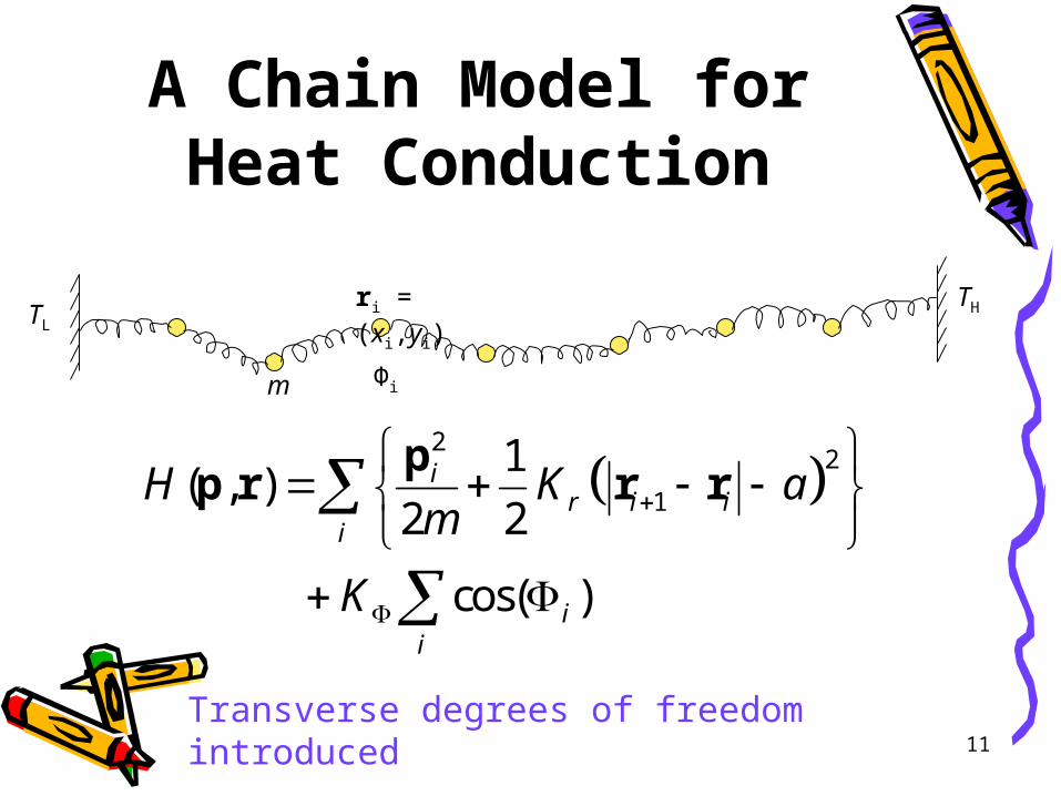
A Chain Model for Heat Conduction
m
ri = (xi,yi)
Φi
2
2
1
1( , )
2 2
cos( )
ir i i
i
ii
H K am
K
pp r r r
TL
TH
Transverse degrees of freedom introduced
12
Nonequilibrium Molecular Dynamics
• Nosé-Hoover thermostats at the ends at temperature TL and TH
• Compute steady-state heat current: j =(1/N)i d (i ri)/dt, where i is local energy associated with particle i
• Define thermal conductance by <j> = (TH-TL)/(Na)
N is number of particles, a is lattice spacing.

13
Nosé-Hoover Dynamics
,
,
,
2,
2,
if
if
if
1 11
i L i w
ii w w
i H i w
L H i
i wB L H w
i Nd
N N i Ndt
i N N
d
dt k T N m
f pp
f
f p
p

14
Defining Microscopic Heat Current
• Let the energy density be
then J satisfies
• A possible choice for total current is
( , ) ( )i ii
t r r r
t
J 0
1
( )( , )
Ni i
iV
dN r t dV
dt
r
j J

15
Expression of j for the chain model
1 1 1
1
22 2
1
1
( ) ( ) ( ) ( 1)
( 2, 1, 1) ( 1, 1, )
1( ) (| | )
4( , , ) ( cos ) / | |
1(| | ) (| | ) cos( )
4 2
i i i i i i i
i i i i i i
r i i
i k j k
ii r i i i
i i
m i i
i i i i i i
i K a
i j k K
K a a Km
j r p p G r p p G
r p H r p H p
G r n
H n n r
pr r
r r r , / | |i i i i n r r
16
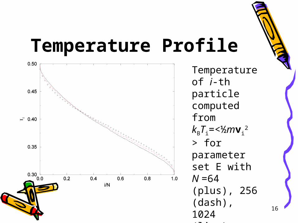
Temperature ProfileTemperature of i-th particle computed from kBTi=<½mvi
2 > for parameter set E with N =64 (plus), 256 (dash), 1024 (line).

17
Conductance vs Size NModel parameters (KΦ, TL, TH):
Set F (1, 5, 7), B (1, 0.2, 0.4), E (0.3, 0.3, 0.5), H (0, 0.3, 0.5), J (0.05, 0.1, 0.2) ,
m=1, a=2, Kr=1.
From J-S Wang & B Li, Phys Rev Lett 92 (2004) 074302.
ln N
slope=1/3
slope=2/5

18
Additional MD dataParameters (KΦ, TL, TH, ε), set L(25,1,1.5,0.2) G(10,0.2,0.4,0) K(0.5,1.2,2,0.4) I(0.1,0.3,0.5,0.2) C(0.1,0.2,0.4,0)
From J-S Wang and B Li, PRE, 70, 021204 (2004).

19
Mode-Coupling Theory for Heat Conduction
• Use Fourier components as basic variables• Derive equations relating the correlation functions
of the variables with the damping of the modes, and the damping of the modes to the square of the correlation functions
• Evoke Green-Kubo formula to relate correlation function with thermal conductivity

20
Basic Variables (work in Fourier space)
2 /
2 /
( ) ,
,
, ( , , , )
1, 2, ,
i kj Nk j
j
i kj Nk j
j
Tk k k k k k
mQ x ja e
N
mQ y e
N
P Q A P P Q Q
k N

21
Equation of Motion for A
Formal solution:
,A H H
LA Lt q p p q
( , , ) ( ( ), ( )) (0, , )tLA t p q A p t q t e A p q
22
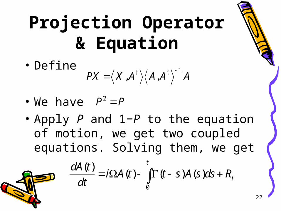
Projection Operator & Equation
• Define
• We have
• Apply P and 1−P to the equation of motion, we get two coupled equations. Solving them, we get
1† †, ,PX X A A A A
2P P
0
( )( ) ( ) ( )
t
t
dA ti A t t s A s ds R
dt

23
Projection Method (Zwanzig and Mori)
• Equation for dynamical correlation function:
where G(t) is correlation matrix of normal-mode Canonical coordinates (Pk,Qk). is related to the correlation of “random” force.
0
( ) ( ) ( ) ( )t
G t t G d i G t
24
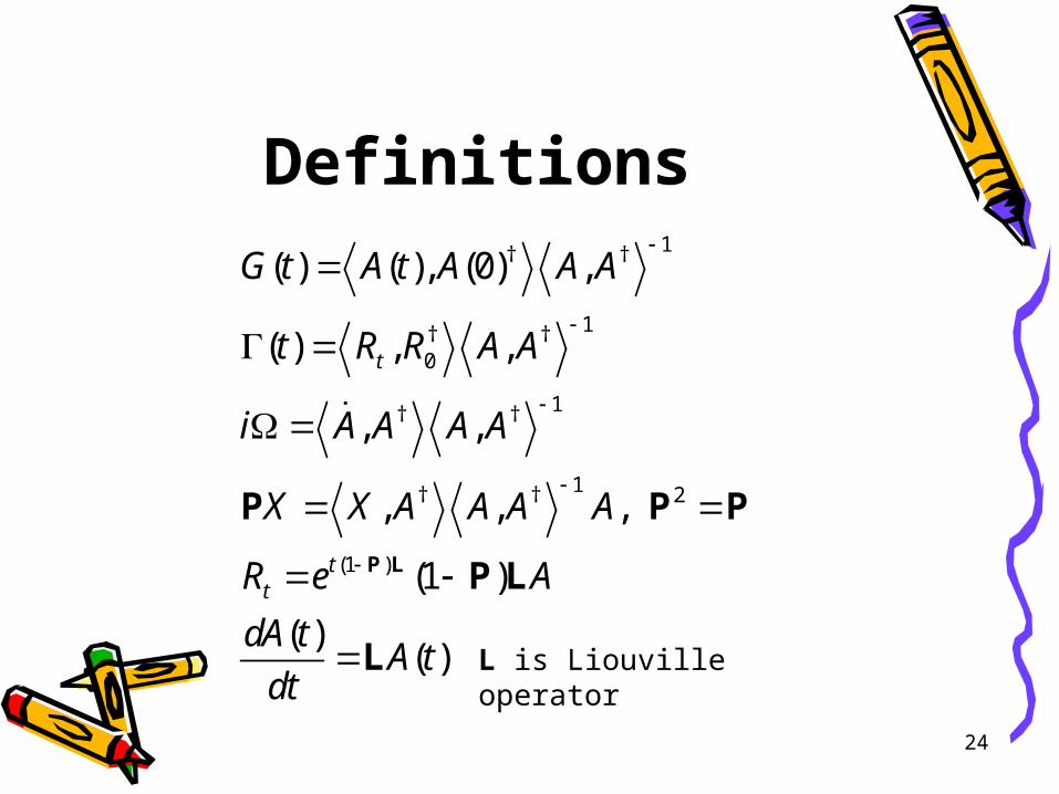
Definitions1† †
1† †0
1† †
1† † 2
(1 )
( ) ( ), (0) ,
( ) , ,
, ,
, , ,
(1 )
( )( )
t
tt
G t A t A A A
t R R A A
i A A A A
X X A A A A
R e A
dA tA t
dt
P L
P P P
P L
L
L is Liouville operator

25
Correlation function equation and its solution (in Fourier-
Laplace space)
• Define
the equation can be solved as
in particular
0
( ) ( ) ( ) ( )t
G t t G d i G t
0
[ ] ( )iztG z e G t dt
1[ ]
( ) [ ]G z
i z z
*
2 220
( ) (0) [ ][ ] , ,
( ) [ ]| |
k k izt kk
k kk
Q t Q iz zg z e dt
z iz zQ

26
Small Oscillation Effective Hamiltonian
2 22
,
(3), , , ,
0
1( , ) ( )
2eff k k kk
k p q k p q k p q k p qk p q
H P Q P Q
v Q Q Q v Q Q Q
, k kk k
H HP Q
Q P
Equations of
motion
27
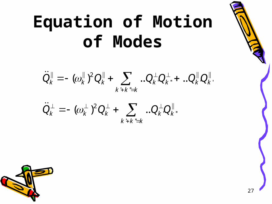
Equation of Motion of Modes
2' '' ' '
' ''
2' ''
' ''
( ) .. ..
( ) ..
k k k k k k kk k k
k k k k kk k k
Q Q Q Q Q Q
Q Q Q Q
28
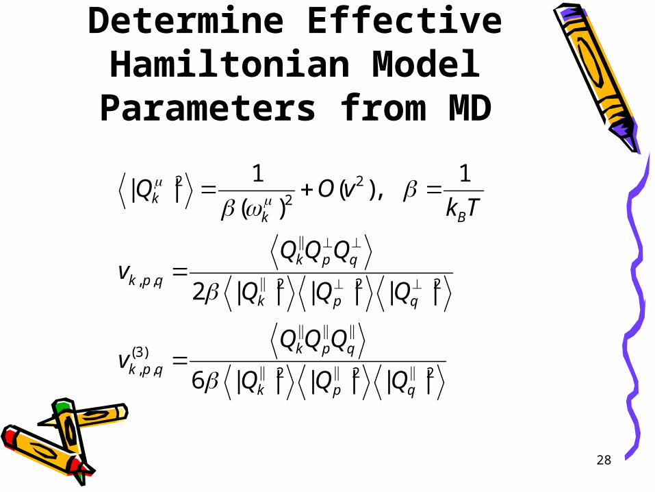
Determine Effective Hamiltonian Model
Parameters from MD
2 22
, , 2 2 2
(3), , 2 2 2
1 1| | ( ),
( )
2 | | | | | |
6 | | | | | |
kk B
k p q
k p q
k p q
k p q
k p q
k p q
Q O vk T
Q Q Qv
Q Q Q
Q Q Qv
Q Q Q

29
Mode-Coupling Approximation
• (t) <R(t) R(0)>
• R Q Q
• (t) <Q(t)Q(t)Q(0)Q(0)>
<Q(t)Q(0)><Q(t)Q(0)>
g(t)g(t) [mean-field type]

30
Full Mode-Coupling Equations
(3), ,
,
2 2
( ) ( ) ( ) ( ) ( ),
( ) ( ) ( ),
[ ][ ] , ,
( ) [ ]
k p q p q p q p qp q k p q k
k p q p qp q k
kk
k k
t K g t g t K g t g t
t K g t g t
iz zg z
z iz z
is Fourier-Laplace transform of [ ]kg z ( )kg t
31
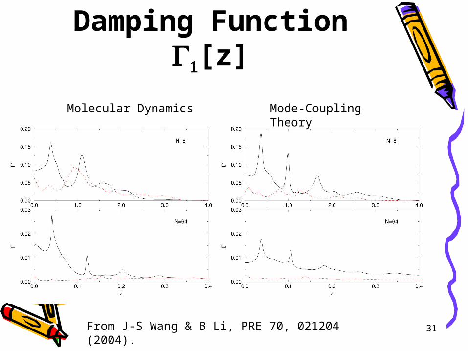
Damping Function [z]
Molecular Dynamics Mode-Coupling Theory
From J-S Wang & B Li, PRE 70, 021204 (2004).

32
Correlation FunctionsCorrelation function g(t) for the slowest longitudinal and transverse modes. Black line: mode-coupling, red dash: MD. N = 256.
g(t) e-tcos(ωt)
33
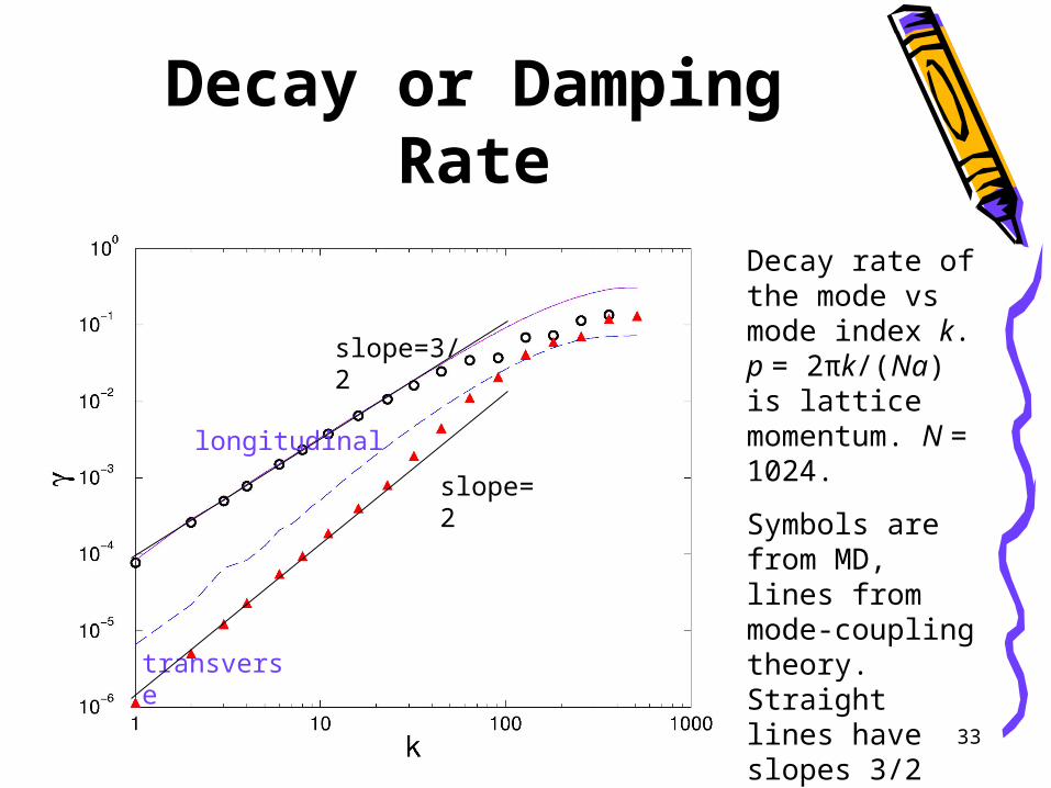
Decay or Damping RateDecay rate of the mode vs mode index k. p = 2πk/(Na) is lattice momentum. N = 1024.
Symbols are from MD, lines from mode-coupling theory. Straight lines have slopes 3/2 and 2, respectively.
longitudinal
transverse
slope=2
slope=3/2
34
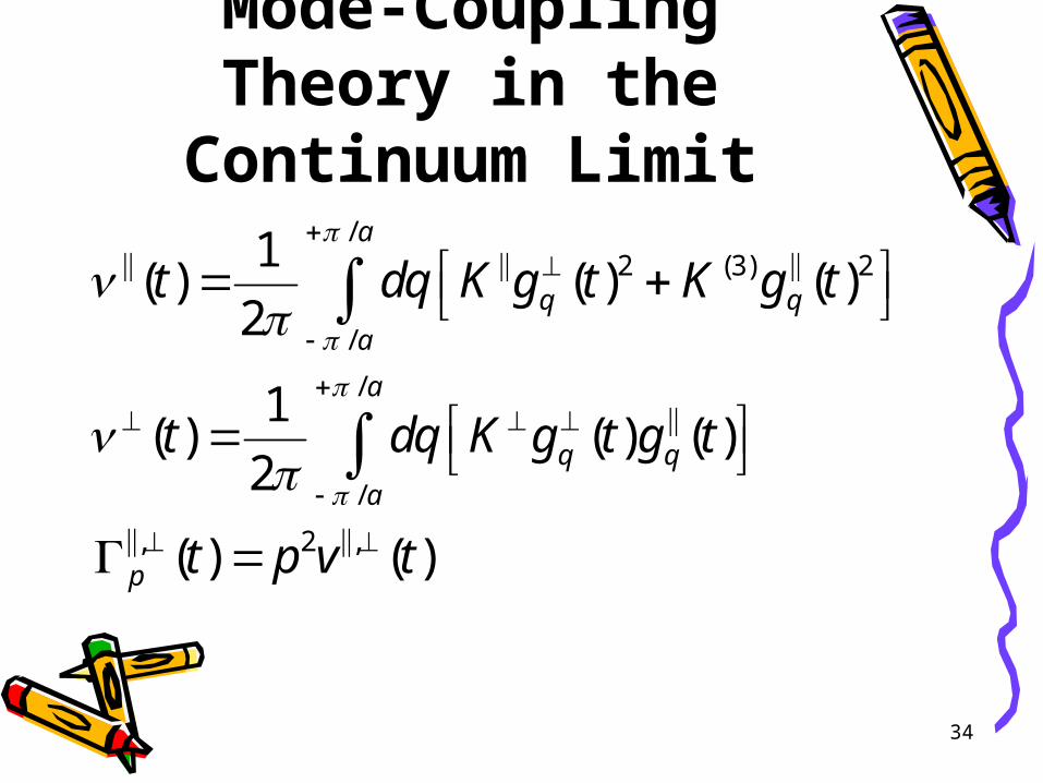
Mode-Coupling Theory in the Continuum Limit
/2 (3) 2
/
/
/
, 2 ,
1( ) ( ) ( )
2
1( ) ( ) ( )
2
( ) ( )
a
q q
a
a
q q
a
p
t dq K g t K g t
t dq K g t g t
t p v t

35
Asymptotic Solution• The mode-coupling equations predict, for
large system size N, and small z :
2
2
2[ ] ,
1[ ] , =
2
p
p
kz c p p
Na
z bz p
If there is no transverse coupling, Γ = z(-1/3)p2 (Result of Lepri).

36
Mode-Coupling [z]/p2
At parameter set B. Blue dash : asymptotic analytical result, red line : Full theory on N =1024, solid line : N limit theory
slope = 0
|| slope = 1/2

37
Green-Kubo Formula
20
*
,
2 2, , ,
,
2
2 1/(2 )
,
1( ) (0) ,
,
( ) (0) | | ( ) ( ) ( )
( )
B
kk k k k k
k
k QQ k PP k QP kk
kk
k k
J t J dtk T aN
J b Q P b ip
J t J b g t g t g t
bg t t
38
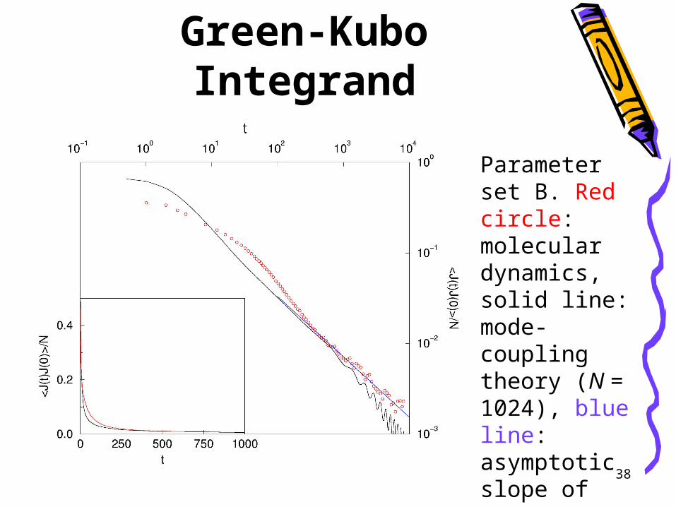
Green-Kubo Integrand
Parameter set B. Red circle: molecular dynamics, solid line: mode-coupling theory (N = 1024), blue line: asymptotic slope of 2/3.
39
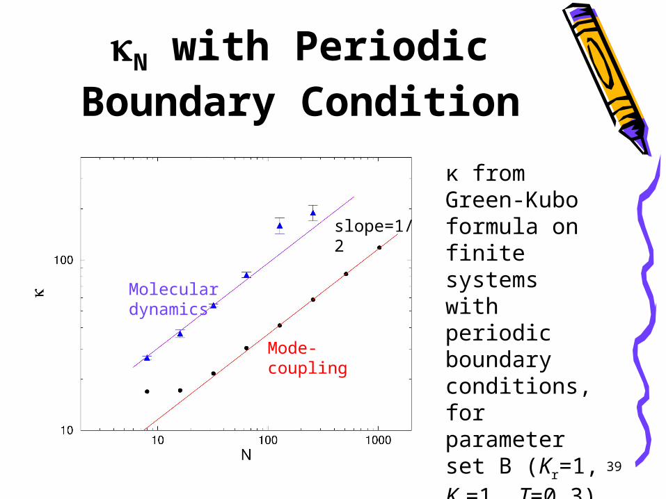
N with Periodic Boundary Condition
κ from Green-Kubo formula on finite systems with periodic boundary conditions, for parameter set B (Kr=1, KΦ=1, T=0.3)
Mode-coupling
Molecular dynamics
slope=1/2

40
Relation between Exponent in Γ and κ
• If mode decay with Γ≈z-δp2, then• With periodic B.C. thermal conductance κ
≈ N 1-δ
• With open B.C. κ ≈ N 1-1/(2-δ)
• Mode coupling theory gives δ=1/2 with transverse motion, and δ=1/3 for strictly 1D system.

41
Conclusion
• Quantitative agreement between mode-coupling theory and molecular dynamics is achieved
• Molecular dynamics and mode-coupling theory support 1/3 power-law divergence for thermal conduction in 1D models with transverse motion, 2/5 law if there are no transverse degrees of freedom.