head and body motion prediction to enable mobile vr

Head and Body Motion Prediction to EnableMobile VR Experiences with Low Latency

Xueshi Hou1, Jianzhong Zhang2, Madhukar Budagavi2, Sujit Dey11University of California, San Diego 2Samsung Research America

[email protected], {jianzhong.z, m.budagavi}@samsung.com, [email protected]

Abstract—As virtual reality (VR) applications become popular,the desire to enable high-quality, lightweight and mobile VR leadsto various edge/cloud-based techniques. This paper introducesa predictive pre-rendering approach to address the ultra-lowlatency challenge in edge/cloud-based six Degrees of Freedom(6DoF) VR. Compared to 360-degree videos and 3DoF (headmotion only) VR, 6DoF VR supports both head and bodymotions, thus not only viewing direction, but also viewing positionchanges. In our approach, the predictive view is rendered inadvance based on the predicted viewing direction and position,leading to a reduction in latency. The key to achieving thisefficient predictive pre-rendering approach is to predict the headand body motion accurately using past head and body motiontraces. We develop a deep learning-based model and validate itsability using a dataset of over 840,000 samples for head and bodymotion.

Index Terms—Virtual reality, video streaming, six Degrees ofFreedom (6DoF).

I. INTRODUCTION

Virtual reality (VR) systems have triggered enormous inter-est over the last few years in various fields including enter-tainment, enterprise, education, manufacturing, transportation,etc. However, several key hurdles need to be overcome forbusinesses and consumers to get fully on board with VRtechnology [1]: cheaper price and compelling content, andmost importantly a truly mobile VR experience. Of particularinterest is how to develop mobile (wireless and lightweight)head-mounted displays (HMDs), and how to enable VR/ARexperience on the mobile HMDs using bandwidth constrainedmobile networks, while satisfying the ultra-low latency re-quirements.

Currently used HMDs can be divided into several cate-gories [2]: PC VR, standalone VR, mobile VR. Specifically,PC VR has high visual quality with rich graphics contentsas well as high frame rate, but the HMD is usually tetheredwith PC [3], [4]; standalone VR HMD has a built-in processorand is mobile, but may have relative low-quality graphics andlower refresh rate [5], [6]; mobile VR is with a smartphoneinside, leading to a heavy HMD to wear [7], [8]. Therefore,current HMDs still cannot offer us a lightweight, mobile,and high-quality VR experience. To solve this problem, wepropose an edge/cloud-based solution. By performing therendering on edge/cloud servers and streaming videos tousers, we can complete the heavy computational tasks on theedge/cloud server and thus enable mobile VR with lightweightVR glasses. The most challenging part of this solution areultra-high bandwidth and ultra-low latency requirements, sincestreaming 360-degree video causes tremendous bandwidthconsumption and good VR user experiences require ultra-lowlatency (<20ms) [9], [10].

Specifically, the total end-to-end latency of edge/cloud-based VR system includes following parts: time of transmittingsensor data from HMD to server, time of rendering (and encod-ing) on server, time of transmitting rendered video from serverto HMD, and time of (decoding and) displaying the view onHMD. The encoding and decoding are optional according tothe specific application design. Once the user moves his/her

Rendering TransmissionBaseline

TransmissionProposedApproach Latency Reduced

Rendering TransmissionBaseline

ProposedApproach Latency Reduced

Encoding Decoding

TransmissionEncoding Decoding

(a)

(b)

Fig. 1. Illustration of rendering and streaming pipeline: (a) Withoutencoding and decoding; (b) With encoding and decoding.

head or body position, high-quality VR requires this end-to-end latency as less than 20ms [9], [10] to avoid motionsickness. For edge/cloud-based VR system, it is extremelychallenging to meet this requirement.

Motivated by the latency challenge, in this paper, we pro-pose a novel approach of enabling mobile VR with predictionfor head and body motions to satisfy ultra-low latency require-ment. If we can predict head and body motion of users in thenear future, we can do predictive pre-rendering on the edgedevice and then stream (even pre-deliver) predicted view tothe HMD. Note that both the choices can significantly reducelatency: one does pre-rendering and the other does both pre-rendering and pre-delivery. The latter reduces more latencythan the former but (i) needs a module on HMD to buffer thepredicted view and determine whether the predicted viewingposition and direction are correct; (ii) transmits extra contentwhen prediction is inaccurate. Hence, we adopt the formermethod, where the latency can be significantly reduced sincethe pre-rendered view will be transmitted if the predictedviewing position and direction are ’correct’ (i.e. the error isless than a given ultra-low value); otherwise, latency remainsthe same with traditional streaming method because the actualview will be rendered and transmitted to the HMD. Fig. 1illustrates the latency reduced by our pre-rendering approachcompared to the traditional approach, in terms of rendering andstreaming pipeline (from server to HMD). The key to achiev-ing this efficient predictive pre-rendering approach is solvingthe problem of motion prediction stated in Section III.A.

In our earlier work [11], we proposed techniques for headmotion prediction in 360-degree videos and three Degreesof Freedom (3DoF) VR applications. In this work, we areaddressing the problem of both head and body motion pre-diction in six Degrees of Freedom (6DoF) VR applications.Compared to 360-degree videos and 3DoF VR (support onlyhead motion), 6DoF VR supports both head and body motion.For head motion prediction in 360-degree videos and 3DoFVR, a certain prediction error is allowed, because the errorcan be handled by delivering larger field of view (FOV) withhigh quality or rendering larger FOV. However, the motionprediction in 6DoF VR is much more challenging, where thebody motion prediction needs high precision to pre-render theuser’s view (otherwise may cause dizzy feeling). For 360-degree videos and 3DoF VR, the 360-degree view at a time

To appear in 2019 IEEE Global Communications Conference (GLOBECOM'19), Waikoloa, HI, USA, Dec. 2019.

1

point is known and unchanged by any head motion, but for6DoF VR it can be totally different due to the body motion.Therefore, this paper will explore the feasibility of doingmotion prediction with high precision in 6DoF VR, and itsmain contributions can be summarized as follows:

• For 6DoF VR applications, we propose a new predic-tive pre-rendering approach involving both body andhead motion prediction, in order to enable high-quality,lightweight, and mobile VR with low latency.

• We develop a prediction method using deep learningto predict where a user will be standing (i.e. viewingposition) and looking into (i.e. viewing direction) in the360-degree view based on their past behavior. Using adataset of real head motion traces from VR applications,we show the feasibility of our long short-term memory(LSTM) model for body motion prediction and multi-layer perceptron (MLP) model for head motion predictionwith high precision.

• To the best of our knowledge, we are the first to comeup with this predictive pre-rendering idea for 6DoF VRapplications and show good results on a real motiontrace dataset in the VR applications. We demonstrate thepotential of our approach with high accuracy of head andbody motion prediction.

The rest of the paper is organized as follows. §2 reviewsrelated work. §3 presents the system overview and problemdefinition. §4 describes our dataset. The methodology for headand body motion prediction is described in §5. We present ourexperimental results in §6, and conclude our work in §7.

II. RELATED WORK

In this section, we review current work in the followingtopics related to our research.

Enable High-Quality Mobile VR: Some recent stud-ies [12]–[14] explore solutions to enable lightweight andmobile VR experiences, and improve the performance ofcurrent VR system. To provide high-quality VR on mobiledevice, [12] presents a pre-rendering and caching design calledFlashBack, which pre-renders all possible views for differentpositions as well as orientations, stores them on a local cache,and delivers frames on demand according to current positionand orientations. Due to infinite choices for different position,they propose to only render the view at each 3D grid point(grid density is 2-5cm). This may bring high inaccuracy anderror to the VR system, leading to negative user experiences.Pre-caching all possible views will also cause overwhelmingstorage overhead (e.g. 50GB for an app). In contrast, ourmethod aims to do a predictive pre-rendering based on headand body motion predictions, thus eliminating the above erroras well as overwhelming storage overhead. [13] introduces aparallel rendering and streaming mechanism to reduce the add-on streaming latency, by pipelining the rendering, encoding,transmission and decoding procedures. Their method focuseson minimizing streaming latency, thus the latency for ren-dering part remains the same with traditional method. [14]presents a collaborative rendering method to reduce overallrendering latency by offloading costly background renderingto a server and only performing foreground rendering on themobile device. This method reduces the rendering latency tosome extent. In contrast, our method propose to pre-renderbased on head and body motion predictions, reducing thelatency of rendering more drastically.

Human Motion Prediction: Learning statistical modelsof human motion is challenging due to the stochastic natureof human movement to explore the environment, and manywork [15]–[19] propose methods to address it. Based on

classical mechanics, there are some studies [15]–[17] showingthe efficiency of linear acceleration model (Lin-A) by doingmotion prediction or estimation with assumption of linearacceleration, especially in a small time interval (e.g. order oftens of milliseconds). [15] describes a good performance of asimple first-order linear motion model for tracking human limbsegment orientation, and [16], [17] reveal acceptable resultswhen employing the linear model as a baseline to predicthuman trajectory. Meanwhile, deep learning approaches [16]–[19] for human body prediction have also achieved remarkableaccomplishments. Specifically, [16], [17] propose their LSTMmodels to predict human future trajectories, but their modelsaim to learn general human movement from massive num-ber of videos and the corresponding precision of predictedposition is much lower than needed for pre-rendering in VRscenarios. [18], [19] propose various recurrent neural network(RNN) models for human motion prediction to learn humankinematics from skeletal data. But these models are complexbecause of being designed to learn the patterns from a seriesof skeletal data and predict as long as 80ms ahead.

Moreover, [20]–[23] also explore the feasibility of doinghead motion prediction, however, head motion prediction in6DoF is quite different than 360-degree video (3DoF), sincein the latter for each time point, the whole 360-degree viewdisplayed for viewers is fixed and more regularity and patternexist in their viewing directions. By learning viewers’ traces,for 3DoF applications, the models can well predict the viewingposition since at a certain time point, there are always someareas attracting most attention and viewers are more likely tolook at them. Head motion in 6DoF is more difficult to predictbecause both position and viewing direction may continuouslychange, and there is a much larger virtual space to explorefor users. Therefore, the above approaches cannot be used toaddress our scenario: we aim to explore high-precision humanbody and head motion prediction in 6DoF VR applications forthe purpose of pre-rendering.

III. SYSTEM OVERVIEW

In this section, we describe our system overview. In ourproposed system, a user’s head motion, body motion as wellas other controlling commands will firstly be sent to the edgedevice, which performs the predictive pre-rendering approach.Based on the past few seconds of head motion, body motionand control data received from the user, the edge devicewill do three things: (i) perform motion prediction; (ii) dopre-rendering based on the predicted viewing position anddirection; (iii) cache the predicted frames in advance. Later,if the predicted viewing position and direction are ’correct’(i.e. the error is less than a given ultra-low value), the cachedpredicted frames can be streamed from the edge device tothe HMD and displayed on HMD immediately; otherwise,the actual view will be rendered by the edge device andtransmitted to the HMD. For the former case, latency neededwill be significantly reduced since the view is pre-renderedand cached on the edge server before it is needed; for thelatter, latency remains the same with the conventional methodof streaming from the edge server. Note that although thecontroller can affect the rendered frame by pointing at a certainplace to teleport in virtual space, we do not need to predict forthe new location triggered by the controller, as in this case,users will expect much larger latency than 20ms.

Note that the edge device can be either a Mobile EdgeComputing node (MEC) in the mobile radio access or corenetwork, or a Local Edge Computing node (LEC) located inthe user premises or even his/her mobile device, connectingto the HMD through WiFi or WiGig. While each of the above

2

!""#$%

!""#$&

!""#$'

(a)

!"# $%&'()"'*!+# ,"--

!*# ,"-- !.# (.''"$.

!$# /0"--$%&'()"'*

(b)

!

"

#

!"#

$%&'()*++

!

" #

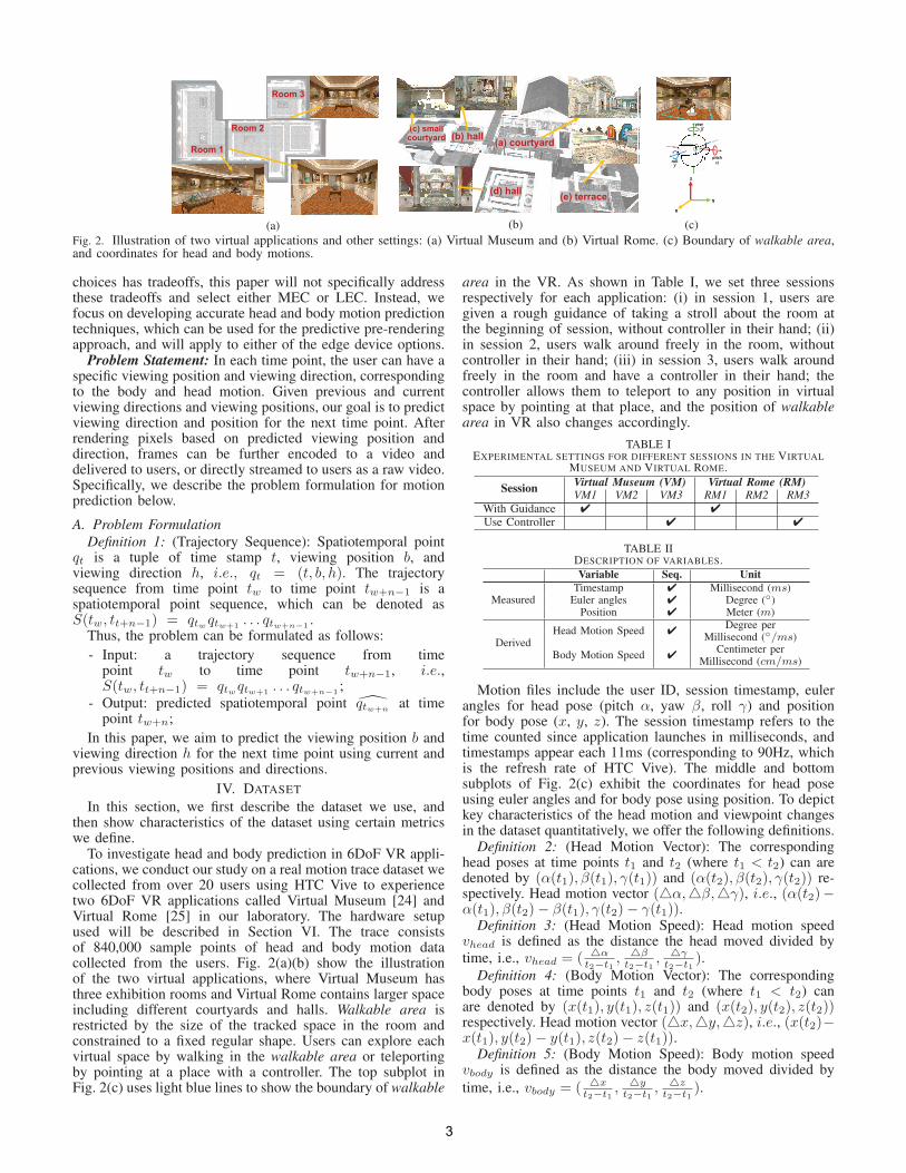
(c)Illustration of two virtual applications and other settings: (a) Virtual Museum and (b) Virtual Rome. (c) Boundary of walkableFig. 2. Illustration of two virtual applications and other settings: (a) Virtual Museum and (b) Virtual Rome. (c) Boundary of walkable area,

and coordinates for head and body motions.

choices has tradeoffs, this paper will not specifically addressthese tradeoffs and select either MEC or LEC. Instead, wefocus on developing accurate head and body motion predictiontechniques, which can be used for the predictive pre-renderingapproach, and will apply to either of the edge device options.

Problem Statement: In each time point, the user can have aspecific viewing position and viewing direction, correspondingto the body and head motion. Given previous and currentviewing directions and viewing positions, our goal is to predictviewing direction and position for the next time point. Afterrendering pixels based on predicted viewing position anddirection, frames can be further encoded to a video anddelivered to users, or directly streamed to users as a raw video.Specifically, we describe the problem formulation for motionprediction below.

A. Problem FormulationDefinition 1: (Trajectory Sequence): Spatiotemporal point

qt is a tuple of time stamp t, viewing position b, andviewing direction h, i.e., qt = (t, b, h). The trajectorysequence from time point tw to time point tw+n−1 is aspatiotemporal point sequence, which can be denoted asS(tw, tt+n−1) = qtwqtw+1

. . . qtw+n−1.

Thus, the problem can be formulated as follows:

- Input: a trajectory sequence from timepoint tw to time point tw+n−1, i.e.,S(tw, tt+n−1) = qtwqtw+1

. . . qtw+n−1;

- Output: predicted spatiotemporal point qtw+nat time

point tw+n;

In this paper, we aim to predict the viewing position b andviewing direction h for the next time point using current andprevious viewing positions and directions.

IV. DATASET

In this section, we first describe the dataset we use, andthen show characteristics of the dataset using certain metricswe define.

To investigate head and body prediction in 6DoF VR appli-cations, we conduct our study on a real motion trace dataset wecollected from over 20 users using HTC Vive to experiencetwo 6DoF VR applications called Virtual Museum [24] andVirtual Rome [25] in our laboratory. The hardware setupused will be described in Section VI. The trace consistsof 840,000 sample points of head and body motion datacollected from the users. Fig. 2(a)(b) show the illustrationof the two virtual applications, where Virtual Museum hasthree exhibition rooms and Virtual Rome contains larger spaceincluding different courtyards and halls. Walkable area isrestricted by the size of the tracked space in the room andconstrained to a fixed regular shape. Users can explore eachvirtual space by walking in the walkable area or teleportingby pointing at a place with a controller. The top subplot inFig. 2(c) uses light blue lines to show the boundary of walkable

area in the VR. As shown in Table I, we set three sessionsrespectively for each application: (i) in session 1, users aregiven a rough guidance of taking a stroll about the room atthe beginning of session, without controller in their hand; (ii)in session 2, users walk around freely in the room, withoutcontroller in their hand; (iii) in session 3, users walk aroundfreely in the room and have a controller in their hand; thecontroller allows them to teleport to any position in virtualspace by pointing at that place, and the position of walkablearea in VR also changes accordingly.

TABLE IEXPERIMENTAL SETTINGS FOR DIFFERENT SESSIONS IN THE VIRTUAL

MUSEUM AND VIRTUAL ROME.

SessionVirtual Museum (VM) Virtual Rome (RM)VM1 VM2 VM3 RM1 RM2 RM3

With Guidance ✔ ✔

Use Controller ✔ ✔

TABLE IIDESCRIPTION OF VARIABLES.Variable Seq. Unit

MeasuredTimestamp ✔ Millisecond (ms)

Euler angles ✔ Degree (◦)Position ✔ Meter (m)

DerivedHead Motion Speed ✔

Degree perMillisecond (◦/ms)

Body Motion Speed ✔Centimeter per

Millisecond (cm/ms)

Motion files include the user ID, session timestamp, eulerangles for head pose (pitch α, yaw β, roll γ) and positionfor body pose (x, y, z). The session timestamp refers to thetime counted since application launches in milliseconds, andtimestamps appear each 11ms (corresponding to 90Hz, whichis the refresh rate of HTC Vive). The middle and bottomsubplots of Fig. 2(c) exhibit the coordinates for head poseusing euler angles and for body pose using position. To depictkey characteristics of the head motion and viewpoint changesin the dataset quantitatively, we offer the following definitions.

Definition 2: (Head Motion Vector): The correspondinghead poses at time points t1 and t2 (where t1 < t2) can aredenoted by (α(t1),β(t1), γ(t1)) and (α(t2),β(t2), γ(t2)) re-spectively. Head motion vector (△α,△β,△γ), i.e., (α(t2)−α(t1),β(t2)− β(t1), γ(t2)− γ(t1)).

Definition 3: (Head Motion Speed): Head motion speedvhead is defined as the distance the head moved divided bytime, i.e., vhead = ( △α

t2−t1, △βt2−t1

, △γt2−t1

).Definition 4: (Body Motion Vector): The corresponding

body poses at time points t1 and t2 (where t1 < t2) canare denoted by (x(t1), y(t1), z(t1)) and (x(t2), y(t2), z(t2))respectively. Head motion vector (△x,△y,△z), i.e., (x(t2)−x(t1), y(t2)− y(t1), z(t2)− z(t1)).

Definition 5: (Body Motion Speed): Body motion speedvbody is defined as the distance the body moved divided by

time, i.e., vbody = ( △xt2−t1

, △yt2−t1

, △zt2−t1

).

3

0 90 180 270 360 450(a) Time points

-0.20

0.20.4

Spee

d (m

/s) vx vx after filtering

0 90 180 270 360 450(b) Time points

-0.5

0

0.5

1

Spee

d (m

/s) vy vy after filtering

0 90 180 270 360 450(c) Time points

-0.2

0

0.2

Spee

d (m

/s) vz vz after filtering

0 90 180 270 360 450(d) Time points

-100

0

100

Spee

d (º/

s)

v v after filtering

0 90 180 270 360 450(e) Time points

-200

0

200

400

Spee

d (º/

s)

v v after filtering

0 90 180 270 360 450(f) Time points

-50

0

50

Spee

d (º/

s)

v v after filtering

Fig. 3. Motion speed obtained before and after the preprocess: (a)(b)(c) for body motion; (d)(e)(f) for head motion.

Table II presents the description of variables. Apart frommeasured variables in the dataset, for each sample point, wecan obtain the derived variables including head motion speedand body motion speed using definitions above.

V. OUR APPROACH

In this section, we describe our proposed approach ofpreprocessing and modeling for head and body motion pre-dictions.

Preprocess: We aim to remove noise within head and bodymotion in the preprocessing procedure. We first calculate headmotion speed and body motion speed for each time point.Fig. 3 presents the body motion and head motion speed inx, y, z,α,β, γ axis respectively for a sample in the motiontrace of one user in Virtual Museum. The blue line in eachsubplot shows there can be at times significant noise in eachof motion speed, due to sensor noise and other measuringerror from HTC Vive HMD and base stations. This noise iseasy to identify since the speed cannot change so rapidlyand intensively within several milliseconds. To remove thenoise in body motion and head motion, we propose to usethe Savitzky-Golay filter method [26] because of its efficiencyand high speed. This filter approximates (i.e. least-squarefitting) the underlying function within the moving window bya polynomial of higher order. The blue and red lines in Fig.4 show the speed before and after the preprocessing. We cansee the noise is eliminated after the filtering.

Predictive Model: For motion features, we select 60 timepoints as the prediction time window (i.e. predict head andbody speed according to speed traces in the latest 60 timepoints), since it achieves better performance than 40, 50, 70,80, 90 time points based on our experiments. For training themodel, we choose a simple representation for motion as a1×60 vector, where each element equals to i when the speedis i at that time point, and the dimension of 60 corresponds to60 time points. With this representation, we can obtain motionfeatures from previous and current motion speed.

...LSTMUnit

Predicted Speed

LSTMUnit

LSTMUnit

LSTMUnit

LSTMUnit

Motion Features

LSTMUnit

Fully Connected Layer

...

... Encoder

Decoder

Encoded Vector

...

Motion Features

Predicted Speed

Fully Connected Layer

Fully Connected Layer...

...

(a)† (b)

Fig. 4. (a) LSTM model and (b) MLP model used for motionprediction.

- LSTM Model: Inspired by the success of the RNNEncoder-Decoder in modeling sequential data [27] and good

! !

!

"#$%"#$%

!!"#

"!"##!

$%&&'()*!+!'

,'--)*!+!'!!

"!

"!

&

&

&

'

$! %!

&!

('./+-)('!01/2-+3'/

41%(!0%*')14'/+!%1(

,1(,+!'(+!%1(

Fig. 5. The structure of LSTM unit.

performance of LSTM to capture transition regularities of hu-man movements since they have memory to learn the temporaldependence between observations [28], [29], we implementan Encoder-Decoder LSTM model which can learn generalbody motion as well as head motion patterns, and predict thefuture viewing direction and position based on the past traces.Fig. 4(a) shows the LSTM model we designed and used inour training, where first and second LSTM layers both consistof 60 LSTM units, and the fully connected layer contains1 interconnected node. Our Encoder-Decoder LSTM modelpredicts what the motion speed will be for next time point,given the previous sequence of motion speed. The outputs arethe values of predicted speed for next time point. Note thatthe settings including 60 LSTM units and 60 time points aswindow length are selected during experiments and proved tobe good by empirical results. For the head and body motionprediction, we use the mean square error (MSE) as our lossfunction:

Loss =1

|Ntrain|

∑

y∈Strain

L∑

t=1

(yt − yt)2,

where |Ntrain| is the number of total time steps of all trajec-tories on the train set Strain, and L is the total length of eachcorresponding trajectories. The proposed LSTM model learnsparameters by minimizing mean square error and training isterminated after 50 epochs in our experiments.

Specifically, encoder and decoder sections work as follows.Given the input sequence X = (x1, . . . ,xt, . . . ,xT ) withxt ∈ Rn, where n is the number of driving series (e.g.dimension of feature representation), the encoder learns amapping from xt to ht with

ht = f(ht−1,xt),

where ht ∈ Rm is the hidden state of the encoder at timet, m is the size of the hidden state, and f is a non-linearactivation function of LSTM unit. As shown in Fig. 5, eachLSTM unit has (i) a memory cell with the cell state st, and(ii) three sigmoid gates to control the access to memory cell

4

(forget gate ft, input gate it and output gate ot). We followthe LSTM structure from [27], [30]:

ft = σ(Wf [ht−1;xt] + bf ),

it = σ(Wi[ht−1;xt] + bi),

ot = σ(Wo[ht−1;xt] + bo),

st = ft ⊙ st−1 + it ⊙ (tanh(Ws[ht−1;xt] + bs)),

ht = ot ⊙ tanh(st),

where [ht−1;xt] ∈ Rm+n is a concatenation of the previoushidden state ht−1 and current input xt. Wf , Wi, Wo, Ws ∈Rm×(m+n) as well as bf , bi, bo, bs ∈ Rm are parameters tolearn. Notations of σ and ⊙ are the logistic sigmoid functionand element-wise multiplication. After reading the end of inputsequence sequentially and updating the hidden state as above,the hidden state of LSTM is a summary (i.e. encoded vectorc) of the whole input sequence. Subsequently, the decoder istrained to generate the target sequence (y1, . . . , yt, . . . , yT ) bypredicting yt given hidden state dt of LSTM units in decoderat timestep t. Note that yt ∈ R, and dt ∈ Rp, where p is thesize of the hidden state in decoder. The update of hidden stateis denoted by

dt = f(dt−1, yt−1, c).

Since the nonlinear function is the LSTM unit function,similarly, dt can be updated as:

f ′

t = σ(W ′

f [dt−1; yt−1; c] + b′f ),

i′t = σ(W ′

i [dt−1; yt−1; c] + b′i),

o′

t = σ(W ′

o[dt−1; yt−1; c] + b′o),

s′t = f ′

t ⊙ s′t−1 + i′t ⊙ (tanh(W ′

s[dt−1; yt−1; c] + b′s)),

dt = o′

t ⊙ tanh(s′t),

where [dt−1; yt−1; c] ∈ Rp+m+1 is a concatenation of theprevious hidden state dt−1, decoder input yt−1, and encodedvector c. W ′

f , W ′

i , W ′

o, W ′

s ∈ Rp×(p+m+1) as well as b′f , b′i,b′o, b′s ∈ Rp are parameters to learn. Subsequently, the outputof the decoder is further fed to the fully connected layer.

- MLP Model: Apart from the LSTM model, we proposeto use an MLP [31] model presented in Fig. 4(b) to domotion prediction. Using the same representation and lossfunction described above, this model also takes the motionspeed during the latest 60 time points as input to predict themotion speed for next time point. The MLP model containstwo fully-connected layers with 60 and 1 interconnected nodesrespectively for training. We build up models for body motionand head motion speed in x, y, z,α,β, γ axis respectively.Given the current and previous speed traces, our predictivemodels can predict the speed for next time point and thuspredict the viewing position b and viewing direction h fornext time point (described in Section III.A).

HMD with Wireless Adaptor

Server with Nvidia GeForce RTX 2060

and WiGig Card

Link Box

Video

Controlling Command Controller

Head & Body Motion

Fig. 6. Hardware setup.

TABLE IIIDATASET STATISTICS.

VirtualSession

#Samples #SamplesApplication for Training for Testing

MuseumVM1 41,600 10,354VM2 80,484 20,076VM3 195,197 48,754

RomeRM1 24,912 6,183RM2 48,586 12,103RM3 280,540 70,091

VI. EXPERIMENTAL RESULTS

The hardware setup of our experiments is shown in Fig. 6,where the rendering server is an Intel Core i7 Quad-Coreprocessor with GeForce RTX 2060. It is equipped with aWiGig card connecting with the HTC Vive’s link box using acable. This link box will be within user’s room and transmitrendered frames in a video format from the server to theHMD. On the user side, there are the link box and two HTClighthouse base stations in the room. User will wear a HTCVive HMD equipped with Vive wireless adaptor [32], and usea controller if needed. Note the wireless adaptor and link boxaim to transmit and receive the rendered frames using WiGigcommunications, while the HTC lighthouse base stations areset for capturing 6DoF motions (e.g. including head and bodymotion). The walkable area is around 3m×3m of free space inour experiments, which cannot exceed 4.5m×4.5m since themaximum distance between base stations is 5m [33]. All headand body motions on HMD can be captured accurately usingthis HTC Lighthouse tracking system while controller detectsuser’s controlling commands. For software implementation, weimplement our proposed techniques based on SteamVR SDK[34], OpenVR SDK [35] as well as the Unity game engine [36]for data collection, and use Keras [37] in Python for motionprediction.

We use 80% of the dataset for training the prediction model,and 20% for testing, ensuring the test data is from viewerswhich are different than those in training data. Table IIIpresents the number of samples used as training data andtesting data for each type of session of the two applicationsVirtual Museum and Virtual Rome (described in Section IVand listed in Table I).

Evaluation Metrics: We choose several popular metrics insequential modeling to evaluate performance on our predictiontask:

• Root Mean Square Error (RMSE):

RMSE =

√

√

√

√

1

|Ntest|

∑

y∈Stest

L∑

t=1

(yt − yt)2,

• Mean Absolute Error (MAE):

MAE =1

|Ntest|

∑

y∈Stest

L∑

t=1

(yt − yt),

where |Ntest| is the number of total time steps of all trajecto-ries on the test set Stest.

Baselines: We consider the following baselines to compareagainst the performance of our proposed model:

• Linear Acceleration Model (Lin-A): Following thework of [15]–[17], we compare against this linear regres-sion model, which extrapolates trajectories with assump-tion of linear acceleration. The Lin-A model employs themotion speed at the latest 3 time points to predict theexpected motion speed.

• Equal Acceleration Model (Eql-A): The Eql-A modelis our modified version of Lin-A, where we assume the

5

TABLE IVBODY MOTION PREDICTION FOR VIRTUAL MUSEUM.

Session Modeldx (mm) dy (mm) dz (mm)

RMSE MAE RMSE MAE RMSE MAE

VM1Lin-A 0.139 0.068 0.167 0.061 0.030 0.018

(w/ Guidance;Eql-A 0.079 0.037 0.096 0.033 0.021 0.013

w/o Controller)MLP 0.083 0.051 0.080 0.037 0.025 0.018

LSTM 0.061 0.035 0.074 0.030 0.019 0.013

VM2Lin-A 0.094 0.045 0.099 0.041 0.048 0.021

(w/o Guidance;Eql-A 0.053 0.025 0.056 0.023 0.029 0.013


LSTM 0.039 0.021 0.046 0.029 0.026 0.013

VM3Lin-A 0.063 0.035 0.074 0.037 0.024 0.015

(w/o Guidance;Eql-A 0.036 0.020 0.042 0.022 0.017 0.011

w/ Controller)MLP 0.032 0.021 0.034 0.021 0.017 0.012

LSTM 0.032 0.021 0.033 0.019 0.015 0.010

TABLE VHEAD MOTION PREDICTION FOR VIRTUAL MUSEUM.

Session Modeldα (′) dβ (′) dγ (′)


VM1Lin-A 0.64 0.34 0.96 0.43 0.48 0.21

(w/ Guidance;Eql-A 0.47 0.29 0.57 0.27 0.33 0.18


LSTM 0.44 0.28 0.54 0.30 0.30 0.17

VM2Lin-A 0.80 0.35 1.31 0.52 0.41 0.23

(w/o Guidance;Eql-A 0.49 0.27 0.78 0.34 0.32 0.19


LSTM 0.66 0.34 0.72 0.42 0.55 0.28

VM3Lin-A 0.61 0.35 1.38 0.61 0.33 0.21

(w/o Guidance;Eql-A 0.45 0.29 0.82 0.39 0.26 0.17

w/ Controller)MLP 0.41 0.27 0.66 0.37 0.22 0.15

LSTM 0.48 0.30 0.99 0.55 0.28 0.17

acceleration is approximately equal during a small timeinterval (e.g. 22ms). The advantage of this modificationis as follows: by employing a smaller number of timepoints, the acceleration estimated may approach more theactual value for the following 11ms, than is achieved bythe Lin-A model. We implement the Eql-A model usingmotion speed at the latest 2 time points to predict theexpected motion speed of next time point.

Tables IV, V, VI, and VII exhibit the results of our bodymotion and head motion prediction for the two applicationsrespectively. Specifically, for results of body motion predictionin Tables IV and VI we give the distance between actual andpredicted body position in x, y, z axis (denoted as dx, dy, dz),while for results of head motion prediction in Tables V and VIIwe present the angular distance between actual and predictedhead pose in α,β, γ axis (denoted as dα, dβ , dγ). Note thatwe use MSE as the loss function when doing training. In eachtable, we compare four models and can make the followingobservations:

• Tables IV and VI, which report on the accuracy of bodymotion prediction, show that our LSTM model achievessmallest RMSE in each session and smallest MAE inmost sessions except VM2 compared to Lin-A, Eql-A,and MLP models. It demonstrates the effectiveness ofusing our proposed LSTM model to predict body motionpositions.

• Tables V and VII, which report on the accuracy of headmotion prediction, show that while the LSTM model hassmallest RMSE for session 1, the MLP model performsbetter (results in smaller RMSE) than other three modelsin sessions 2 and 3 for both the applications. Comparedto session 1 (where users take a stroll about the room andhave a relatively fixed trajectory), sessions 2 and 3 aremore general and closer to normal 6DoF VR scenario.Thus, we can see that MLP is a more feasible model todo head motion prediction in general cases.

We can observe that (i) LSTM model achieves a better

TABLE VIBODY MOTION PREDICTION FOR VIRTUAL ROME.

Session Modeldx (mm) dy (mm) dz (mm)


RM1Lin-A 0.174 0.086 0.299 0.084 0.046 0.022

(w/ Guidance;Eql-A 0.100 0.051 0.172 0.047 0.031 0.017


LSTM 0.032 0.021 0.073 0.044 0.024 0.019

RM2Lin-A 0.125 0.053 0.145 0.048 0.036 0.020

(w/o Guidance;Eql-A 0.074 0.032 0.085 0.030 0.025 0.015


LSTM 0.058 0.030 0.065 0.032 0.025 0.015

RM3Lin-A 0.074 0.041 0.077 0.041 0.034 0.019

(w/o Guidance;Eql-A 0.044 0.025 0.046 0.025 0.023 0.013

w/ Controller)MLP 0.040 0.025 0.041 0.026 0.077 0.040

LSTM 0.040 0.024 0.040 0.024 0.023 0.013

TABLE VIIHEAD MOTION PREDICTION FOR VIRTUAL ROME.

Session Modeldα (′) dβ (′) dγ (′)


RM1Lin-A 0.71 0.47 1.32 0.61 0.40 0.27

(w/ Guidance;Eql-A 0.55 0.38 0.79 0.39 0.30 0.21


LSTM 0.53 0.36 0.73 0.47 0.29 0.22

RM2Lin-A 0.92 0.57 2.53 0.66 0.56 0.34

(w/o Guidance;Eql-A 0.66 0.43 1.48 0.44 0.39 0.26


LSTM 0.64 0.43 1.52 0.55 1.23 0.30

RM3Lin-A 0.88 0.50 1.57 0.72 0.44 0.27

(w/o Guidance;Eql-A 0.63 0.38 0.98 0.49 0.33 0.21

w/ Controller)MLP 0.57 0.36 0.82 0.43 0.28 0.18

LSTM 0.60 0.39 0.89 0.52 0.35 0.25

performance in every session of body motion prediction andsession 1 of head motion prediction. These sessions havea relatively small range (e.g. body motion speed is mostlysmaller than ±1m/s), gradual variation and more regularity.(ii) MLP model performs better in sessions 2 and 3 of headmotion prediction. These two sessions have a large value range(e.g. head motion can be up to ±300◦/s), quicker variationand more frequent fluctuations (e.g. head motion speed vβ hasa large and abrupt change from −180◦/s to 200◦/s within 1s,shown in Fig. 3(e)).

To evaluate the adverse effect on user experience caused bythe prediction error between the actual view and the predictedview which will be pre-rendered and delivered to the user,we propose following metric. Assume that we have two viewsV1 and V2 in the RGB format. Firstly, we convert the RGBimages (V1 and V2) to grayscale intensity images I1 and I2 byeliminating the hue and saturation information while retainingthe luminance [38]. For each pixel i in the grayscale intensityimages, we calculate the difference between the two intensityimages, Idif , as follows.

Idif (i) =

{

I1(i)− I2(i), if I1(i) ≥ I2(i)0, otherwise

(1)

Note that we set the Idif as 0 in the second case of Equation 1,because otherwise the motion change of the same object willbe presented in Idif twice: positive and negative respectively.Thus we only keep the positive one (i.e. the first case inEquation 1) to evaluate the difference between the two views.Fig. 7 presents an example of two views and the correspondingIdif . In Fig. 7(c), we can see that most of pixels in theview have the intensity value of 0 while the residual pixelshave intensity values larger than or equal to 1. We define thepercentage of mismatched pixels as

Rdif =Ndif

Nframe,

6

�!� �"� �#�

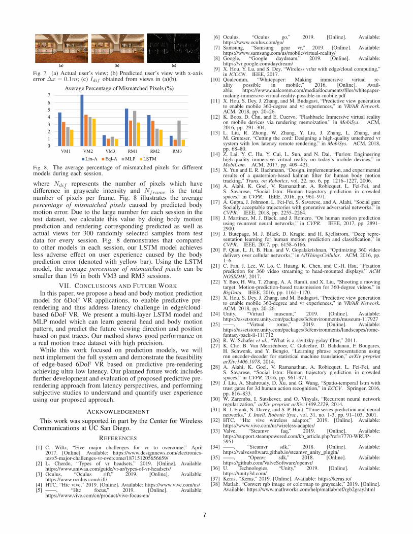
Fig. 7. (a) Actual user’s view; (b) Predicted user’s view with x-axiserror ∆x = 0.1m; (c) Idif obtained from views in (a)(b).

!"#$%&'(

)*" )*# )*$ +*" +*# +*$

,-./01. 2./3.4501. 67 *89:053;.< 28=.>9 ?@A

B84C, DE>C, *B2 BFG*

Fig. 8. The average percentage of mismatched pixels for differentmodels during each session.

where Ndif represents the number of pixels which havedifference in grayscale intensity and Nframe is the totalnumber of pixels per frame. Fig. 8 illustrates the averagepercentage of mismatched pixels caused by predicted bodymotion error. Due to the large number for each session in thetest dataset, we calculate this value by doing body motionprediction and rendering corresponding predicted as well asactual views for 300 randomly selected samples from testdata for every session. Fig. 8 demonstrates that comparedto other models in each session, our LSTM model achievesless adverse effect on user experience caused by the bodyprediction error (denoted with yellow bar). Using the LSTMmodel, the average percentage of mismatched pixels can besmaller than 1% in both VM3 and RM3 sessions.

VII. CONCLUSIONS AND FUTURE WORK

In this paper, we propose a head and body motion predictionmodel for 6DoF VR applications, to enable predictive pre-rendering and thus address latency challenge in edge/cloud-based 6DoF VR. We present a multi-layer LSTM model andMLP model which can learn general head and body motionpattern, and predict the future viewing direction and positionbased on past traces. Our method shows good performance ona real motion trace dataset with high precision.

While this work focused on prediction models, we willnext implement the full system and demonstrate the feasibilityof edge-based 6DoF VR based on predictive pre-renderingachieving ultra-low latency. Our planned future work includesfurther development and evaluation of proposed predictive pre-rendering approach from latency perspectives, and performingsubjective studies to understand and quantify user experienceusing our proposed approach.

ACKNOWLEDGEMENT

This work was supported in part by the Center for WirelessCommunications at UC San Diego.

REFERENCES

[1] C. Wiltz, “Five major challenges for vr to overcome,” April2017. [Online]. Available: https://www.designnews.com/electronics-test/5-major-challenges-vr-overcome/187151205656659/

[2] L. Cherdo, “Types of vr headsets,” 2019. [Online]. Available:https://www.aniwaa.com/guide/vr-ar/types-of-vr-headsets/

[3] Oculus, “Oculus rift,” 2019. [Online]. Available:https://www.oculus.com/rift/

[4] HTC, “Htc vive,” 2019. [Online]. Available: https://www.vive.com/us/[5] ——, “Htc focus,” 2019. [Online]. Available:

https://www.vive.com/cn/product/vive-focus-en/

[6] Oculus, “Oculus go,” 2019. [Online]. Available:https://www.oculus.com/go/

[7] Samsung, “Samsung gear vr,” 2019. [Online]. Available:https://www.samsung.com/us/mobile/virtual-reality/

[8] Google, “Google daydream,” 2019. [Online]. Available:https://vr.google.com/daydream/

[9] X. Hou, Y. Lu, and S. Dey, “Wireless vr/ar with edge/cloud computing,”in ICCCN. IEEE, 2017.

[10] Qualcomm, “Whitepaper: Making immersive virtual re-ality possible in mobile,” 2016. [Online]. Avail-able: https://www.qualcomm.com/media/documents/files/whitepaper-making-immersive-virtual-reality-possible-in-mobile.pdf

[11] X. Hou, S. Dey, J. Zhang, and M. Budagavi, “Predictive view generationto enable mobile 360-degree and vr experiences,” in VR/AR Network.ACM, 2018, pp. 20–26.

[12] K. Boos, D. Chu, and E. Cuervo, “Flashback: Immersive virtual realityon mobile devices via rendering memoization,” in MobiSys. ACM,2016, pp. 291–304.

[13] L. Liu, R. Zhong, W. Zhang, Y. Liu, J. Zhang, L. Zhang, andM. Gruteser, “Cutting the cord: Designing a high-quality untethered vrsystem with low latency remote rendering,” in MobiSys. ACM, 2018,pp. 68–80.

[14] Z. Lai, Y. C. Hu, Y. Cui, L. Sun, and N. Dai, “Furion: Engineeringhigh-quality immersive virtual reality on today’s mobile devices,” inMobiCom. ACM, 2017, pp. 409–421.

[15] X. Yun and E. R. Bachmann, “Design, implementation, and experimentalresults of a quaternion-based kalman filter for human body motiontracking,” Trans. on Robotics, vol. 22, no. 6, pp. 1216–1227, 2006.

[16] A. Alahi, K. Goel, V. Ramanathan, A. Robicquet, L. Fei-Fei, andS. Savarese, “Social lstm: Human trajectory prediction in crowdedspaces,” in CVPR. IEEE, 2016, pp. 961–971.

[17] A. Gupta, J. Johnson, L. Fei-Fei, S. Savarese, and A. Alahi, “Social gan:Socially acceptable trajectories with generative adversarial networks,” inCVPR. IEEE, 2018, pp. 2255–2264.

[18] J. Martinez, M. J. Black, and J. Romero, “On human motion predictionusing recurrent neural networks,” in CVPR. IEEE, 2017, pp. 2891–2900.

[19] J. Butepage, M. J. Black, D. Kragic, and H. Kjellstrom, “Deep repre-sentation learning for human motion prediction and classification,” inCVPR. IEEE, 2017, pp. 6158–6166.

[20] F. Qian, L. Ji, B. Han, and V. Gopalakrishnan, “Optimizing 360 videodelivery over cellular networks,” in AllThingsCellular. ACM, 2016, pp.1–6.

[21] C. Fan, J. Lee, W. Lo, C. Huang, K. Chen, and C.-H. Hsu, “Fixationprediction for 360 video streaming to head-mounted displays,” ACMNOSSDAV, 2017.

[22] Y. Bao, H. Wu, T. Zhang, A. A. Ramli, and X. Liu, “Shooting a movingtarget: Motion-prediction-based transmission for 360-degree videos.” inBigData. IEEE, 2016, pp. 1161–1170.

[23] X. Hou, S. Dey, J. Zhang, and M. Budagavi, “Predictive view generationto enable mobile 360-degree and vr experiences,” in VR/AR Network.ACM, 2018, pp. 20–26.

[24] Unity, “Virtual museum,” 2019. [Online]. Available:https://assetstore.unity.com/packages/3d/environments/museum-117927

[25] ——, “Virtual rome,” 2019. [Online]. Available:https://assetstore.unity.com/packages/3d/environments/landscapes/rome-fantasy-pack-ii-111712

[26] R. W. Schafer et al., “What is a savitzky-golay filter,” 2011.[27] K. Cho, B. Van Merrienboer, C. Gulcehre, D. Bahdanau, F. Bougares,

H. Schwenk, and Y. Bengio, “Learning phrase representations usingrnn encoder-decoder for statistical machine translation,” arXiv preprintarXiv:1406.1078, 2014.

[28] A. Alahi, K. Goel, V. Ramanathan, A. Robicquet, L. Fei-Fei, andS. Savarese, “Social lstm: Human trajectory prediction in crowdedspaces,” in CVPR, 2016, pp. 961–971.

[29] J. Liu, A. Shahroudy, D. Xu, and G. Wang, “Spatio-temporal lstm withtrust gates for 3d human action recognition,” in ECCV. Springer, 2016,pp. 816–833.

[30] W. Zaremba, I. Sutskever, and O. Vinyals, “Recurrent neural networkregularization,” arXiv preprint arXiv:1409.2329, 2014.

[31] R. J. Frank, N. Davey, and S. P. Hunt, “Time series prediction and neuralnetworks,” J. Intell. Robotic Syst., vol. 31, no. 1-3, pp. 91–103, 2001.

[32] HTC, “Htc vive wireless adaptor,” 2019. [Online]. Available:https://www.vive.com/us/wireless-adapter/

[33] Valve, “Steamvr faq,” 2019. [Online]. Available:https://support.steampowered.com/kb article.php?ref=7770-WRUP-5951

[34] ——, “Steamvr sdk,” 2018. [Online]. Available:https://valvesoftware.github.io/steamvr unity plugin/

[35] ——, “Openvr sdk,” 2018. [Online]. Available:https://github.com/ValveSoftware/openvr/

[36] U. Technologies, “Unity,” 2019. [Online]. Available:https://unity3d.com/

[37] Keras, “Keras,” 2019. [Online]. Available: https://keras.io/[38] Matlab, “Convert rgb image or colormap to grayscale,” 2019. [Online].

Available: https://www.mathworks.com/help/matlab/ref/rgb2gray.html

7

head and body motion prediction to enable mobile vr

Documents