HAsim FPGA-Based Processor Models: Multicore Models and Time-Multiplexing

Michael AdlerElliott FlemingMichael PellauerJoel Emer

2

Simulating Multicores

Simulating an N-multicore target•Fundametally N times the work•Plus on-chip network

Duplicating cores will quickly fill FPGAMulti-FPGA will slow simulation

CPU

CPU CPU CPUCPU

CPU CPU CPU CPU

Network

3

Trading Time for Space

Can leverage separation of model clock and FPGA clock to save space

• Two techniques: serialization and time-multiplexing

But doesn’t this just slow down our simulator?

The tradeoff is a good idea if we can:

• Save a lot of space

• Improve FPGA critical path

• Improve utilization

• Slow down rare events, keep common events fast

LI approach enables a wide range of tradeoff options

4

Serialization: A First Tradeoff

5

Example Tradeoff: Multi-Port Register File

2 Read Ports, 2 Write Ports• 5-bit index, 32-bit data

• Reads take zero clock cycles

Virtex 2Pro FPGA: 9242 (>25%) slices, 104 MHz

2R/2WRegister

File

rd addr 1

rd addr 2

wr addr 1wr val 1

wr addr2wr val 2

rd val 1

rd val 2

6

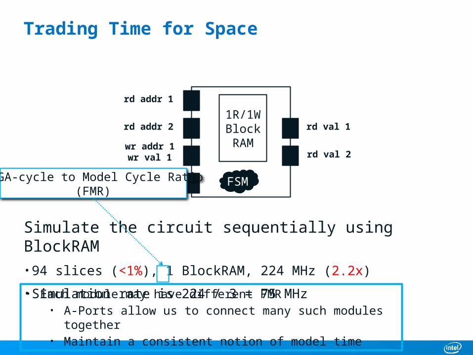
Trading Time for Space

Simulate the circuit sequentially using BlockRAM• 94 slices (<1%), 1 BlockRAM, 224 MHz (2.2x)

• Simulation rate is 224 / 3 = 75 MHz

rd addr 1

rd addr 2

wr addr 1wr val 1

wr addr 2wr val 2

rd val 1

rd val 2

1R/1WBlockRAM

FSM

• Each module may have different FMR• A-Ports allow us to connect many such modules together• Maintain a consistent notion of model time

FPGA-cycle to Model Cycle Ratio(FMR)

7

Example: Inorder Front End

FET

BranchPred

IMEM PCResolve

InstQ

I$

ITLB1 1 1 0

1

2

0

0first

deq

slot

enqor

drop

1

fault

mispred

1training

pred

rspImm

rspDel

1

1redirect

1vaddr

(from Back End)

vaddr

0

(from Back End)

paddr

0paddr

1

LinePred

00

instor

fault

Legend: Ready to simulate?Legend: Ready to simulate?

YesNo

FET

Part

IMEM

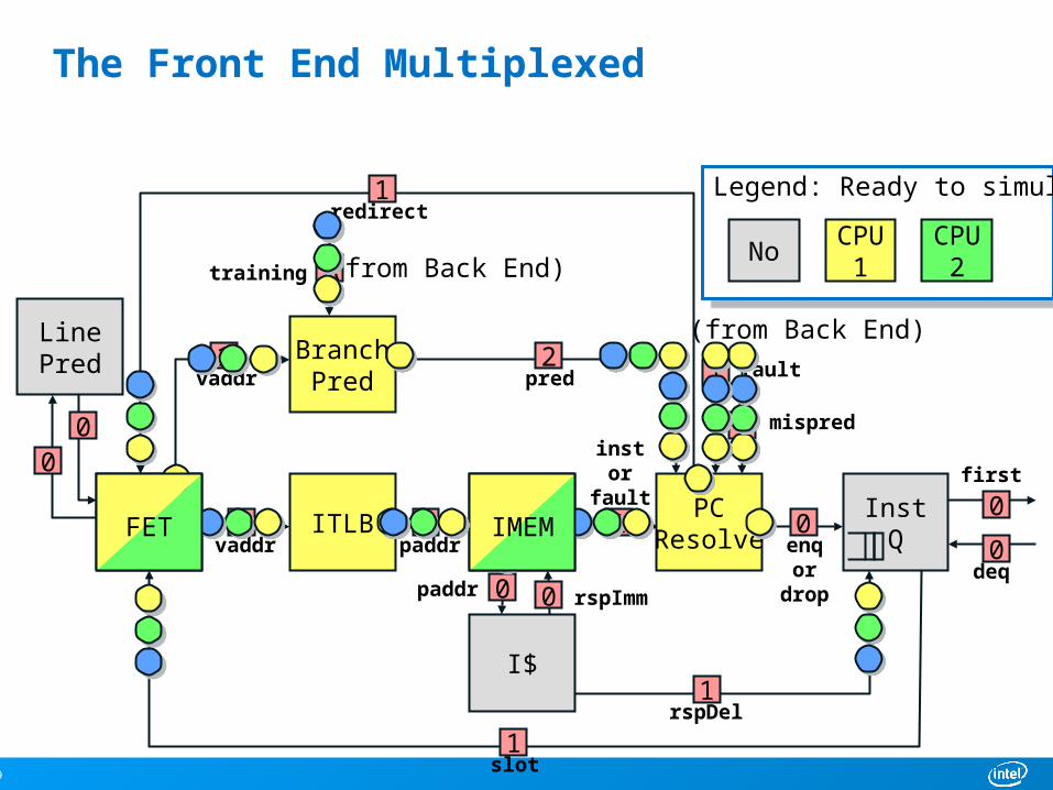
• Modules may simulate at any wall-clock rate• Corollary: adjacent modules may not be simulating the same

model cycle

8

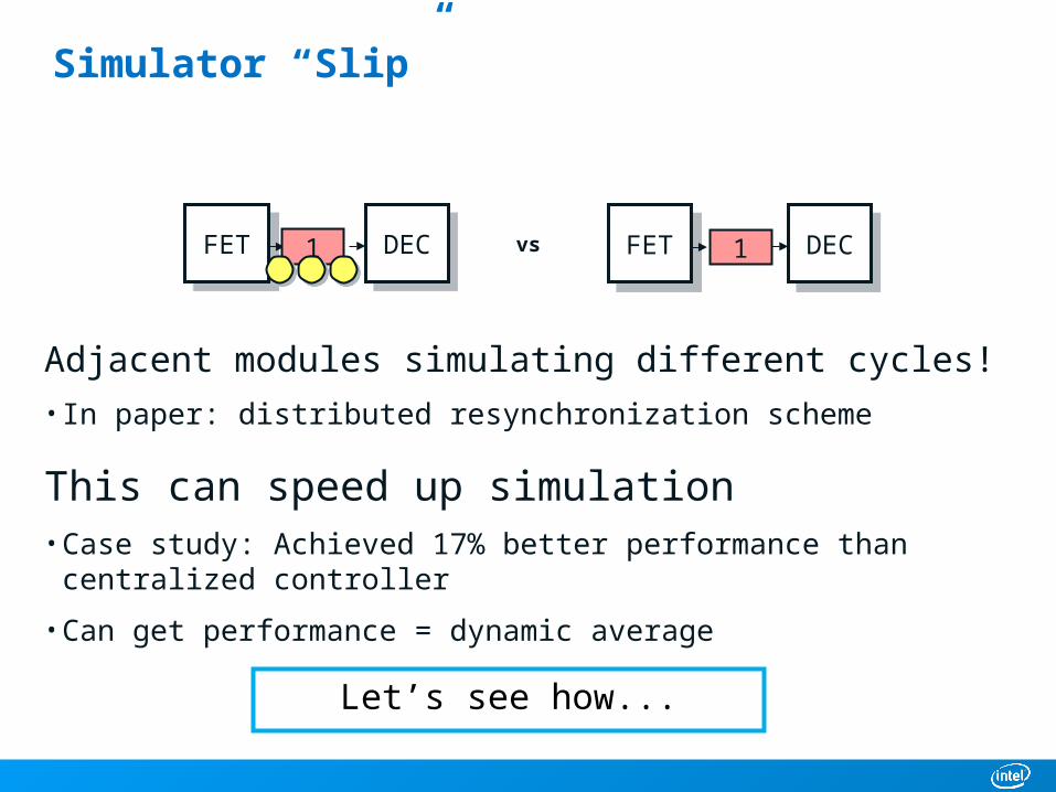
Simulator “Slip”

Adjacent modules simulating different cycles!• In paper: distributed resynchronization scheme

This can speed up simulation• Case study: Achieved 17% better performance than centralized controller

• Can get performance = dynamic average

FETFET DECDEC1FETFET DECDEC1 vs

Let’s see how...

9

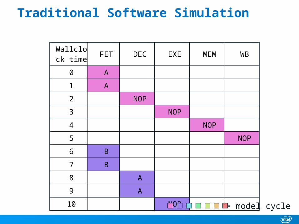
Traditional Software Simulation

Wallclock time

FET DEC EXE MEM WB

0 A

1 A

2 NOP

3 NOP

4 NOP

5 NOP

6 B

7 B

8 A

9 A

10 NOP

= model cycle

10

2008.06.30

Challenges in Conducting Compelling Architecture Research10

Global Controller “Barrier” Synchronization

FPGA CC

FET DEC EXE MEM WB

0 A NOP NOP NOP NOP

1 A

2 A

3 B A NOP NOP NOP

4 B A

5 A

6 C B A NOP NOP

7 B

8 D C B A NOP

9 D

10 D

= model cycle

11

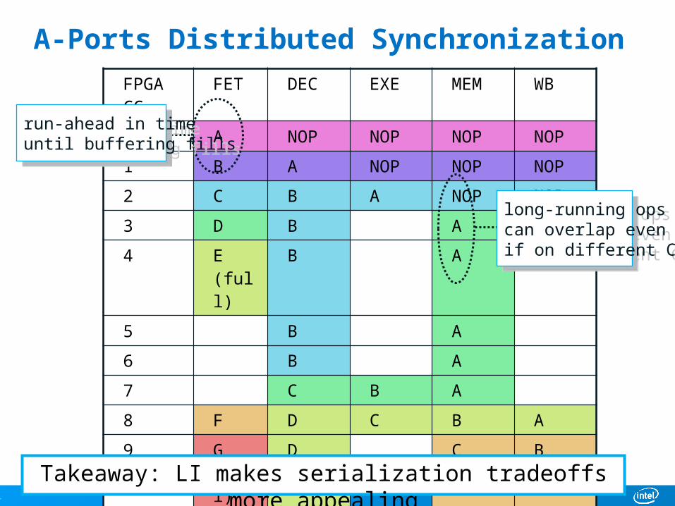
A-Ports Distributed SynchronizationFPGA CC

FET DEC EXE MEM WB

0 A NOP NOP NOP NOP

1 B A NOP NOP NOP

2 C B A NOP NOP

3 D B A NOP

4 E (full)

B A

5 B A

6 B A

7 C B A

8 F D C B A

9 G (full)

D C B

10 D C

11 D

12 D

long-running opscan overlap evenif on different CC

long-running opscan overlap evenif on different CC

run-ahead in timeuntil buffering fills

run-ahead in timeuntil buffering fills

Takeaway: LI makes serialization tradeoffs more appealing

12

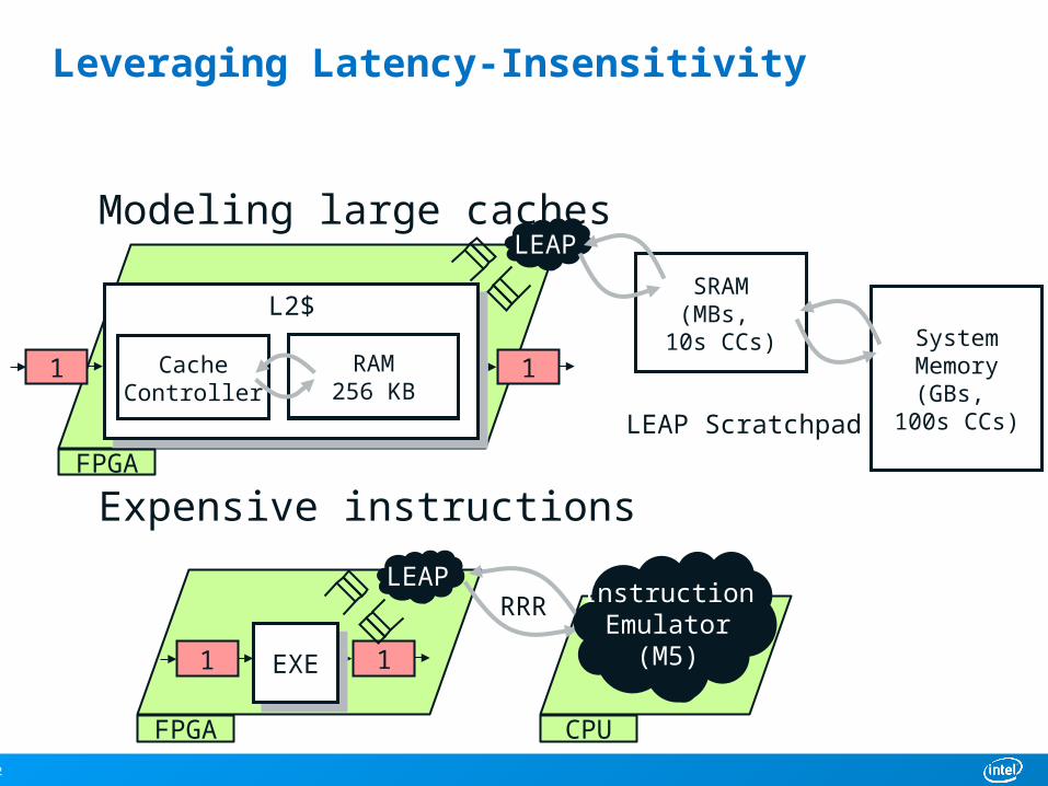
Modeling large caches

Expensive instructions

CPU

Leveraging Latency-Insensitivity

1 1

FPU

EXE

LEAPInstructionEmulator

(M5)

RRR

[With Parashar,

Adler]

FPGA

1 1

L2$

CacheController

BRAM(KBs, 1 CC)

SRAM(MBs,

10s CCs) SystemMemory

(GBs, 100s CCs)

RAM256 KB

FPGA

LEAP

LEAP Scratchpad

13

Time-Multiplexing: A Tradeoff to Scale Multicores

(resume at 3:45)

14

Drawbacks:• Probably won’t fit• Low utilization of functional units

Benefits:• Simple to describe• Maximum parallelism

Multicores Revisited

What if we duplicate the cores?

state state state

CORE 0 CORE 1 CORE 2

15

Module Utilization

FETFET DECDEC1FETFET DECDEC1

A module is unutilized on an FPGA cycle if:• Waiting for all input ports to be non-empty or

• Waiting for all output ports to be non-full

Case Study: In-order functional units were utilized 13% of FPGA cycles on average

1 1

16

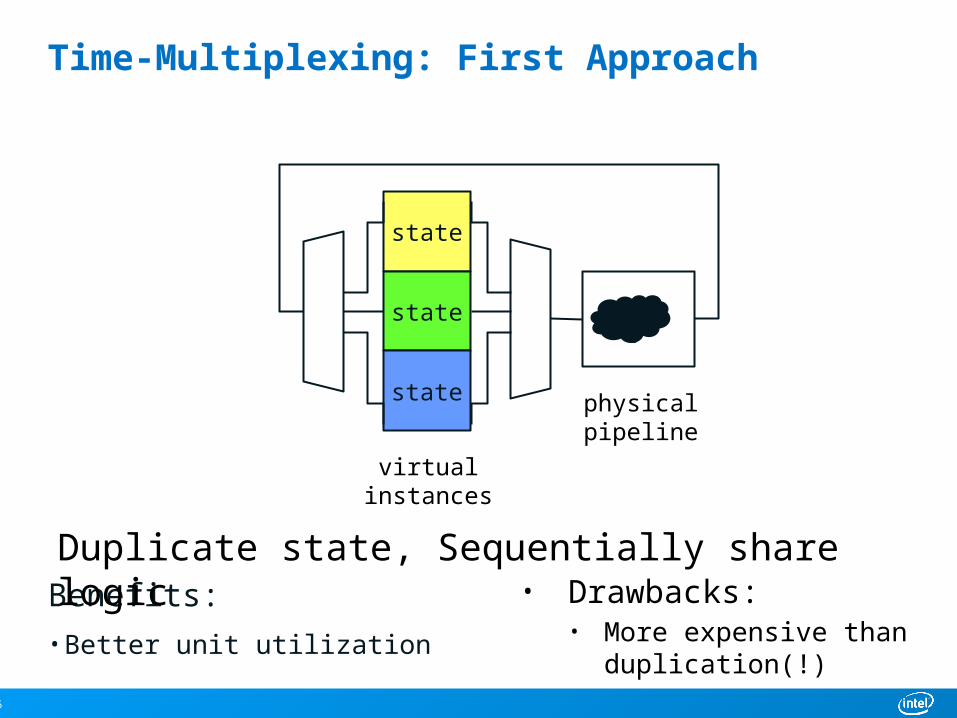
• Drawbacks:• More expensive than

duplication(!)

Benefits:• Better unit utilization

Time-Multiplexing: First Approach

Duplicate state, Sequentially share logic

state

state

state physicalpipeline

virtualinstances

17

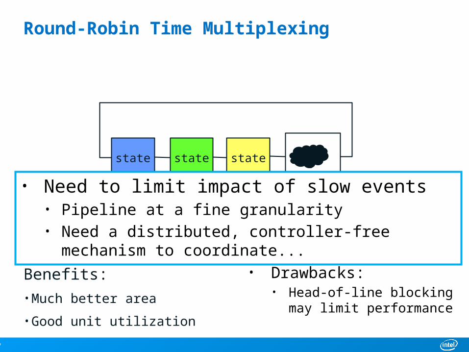
• Drawbacks:• Head-of-line blocking may limit

performance

Benefits:• Much better area

• Good unit utilization

Round-Robin Time Multiplexing

Fix ordering, remove multiplexors

statestatestate

physicalpipeline

• Need to limit impact of slow events• Pipeline at a fine granularity• Need a distributed, controller-free mechanism to coordinate...

18

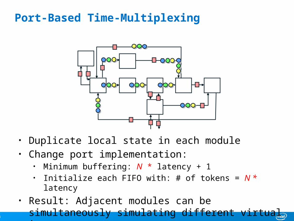
Port-Based Time-Multiplexing

• Duplicate local state in each module• Change port implementation:

• Minimum buffering: N * latency + 1• Initialize each FIFO with: # of tokens = N * latency

• Result: Adjacent modules can be simultaneously simulating different virtual instances

19

The Front End Multiplexed

FET

BranchPred

IMEM PCResolve

InstQ

I$

ITLB1 1 1 0

1

2

0

0first

deq

slot

enqor

drop

1

fault

mispred

1training

pred

rspImm

rspDel

1

1redirect

1vaddr

(from Back End)

vaddr

0

(from Back End)

paddr

0paddr

1

LinePred

00

instor

fault

Legend: Ready to simulate?Legend: Ready to simulate?

CPU1No CPU

2

FET IMEM

20

On-Chip Networks in a Time-Multiplexed World

21

Problem: On-Chip Network

CPUL1/L2 $

msg credit

Memory Control

rr r r

[0 1 2] [0 1 2]

CPU 0L1/L2 $

CPU 1L1/L2 $

CPU 2L1/L2 $

r

router

msg msg

credit credit

• Problem: routing wires to/from each router• Similar to the “global controller” scheme• Also utilization is low

22

Router0..3

Multiplexing On-Chip Network Routers

Router3

Router0

Router2

Router1

cur to 1 to 2 to 3 fr 1 fr 2 fr 30123

0

001

1

1 2 3

2

2 33

reorder

reorder

reorder

σ(x) = (x + 1) mod 4

σ(x) = (x + 2) mod 4

σ(x) = (x + 3) mod 4

1 2 3

0

001

12

2 33

Simulate the network without a network

23

Ring/Double Ring Topology Multiplexed

Router3

Router0

Router2

Router1

Router0..3

“to next”“from prev”

???

cur to N fr P

0

1

2

3

σ(x) = (x + 1) mod 4

1 3

0

012

23

Opposite direction: flip to/from

24

Implementing Permutations on FPGAs Efficiently

Side Buffer•Fits networks like ring/torus (e.g. x+1 mod N)

Indirection Table•More general, but more expensive

PermTable

RAMBuffer

FSM

σ(x) = (x + 1) mod 4

1000 0001

Move first to Nth

Move Nth to first Move every K to N-K

25

Torus/Mesh Topology Multiplexed

Mesh: Don’t transmit on non-existent links

26

Dealing with Heterogeneous Networks

Compose “Mux Ports” with Permutation PortsIn paper: generalize to any topology

27

Putting It All Together

28

Typical HAsim Model Leveraging these Techniques

• 16-core chip multiprocessor• 10-stage pipeline (speculative, bypassed)• 64-bit Alpha ISA, floating point• 8 KB lockup-free L1 caches• 256 KB 4-way set associative L2 cache• Network: 2 v. channels, 4 slots, x-y wormhole

F BP1 BP2 PCC IQ D X DM CQ C

ITLB I$ DTLB D$ L/S Q

L2$ Route

• Single detailed pipeline, 16-way time-multiplexed• 64-bit Alpha functional partition, floating point• Caches modeled with different cache hierarchy• Single router, multiplexed, 4 permutations

Regs LUTs BRAM0%

25%

50%

75%

100%

Synthesis Results, percentage of Xilinx V5 330T

LEAPFuncOCNL1/L2Core

29

Time-Multiplexed Multicore Simulation Rate Scaling

Best Worst Avg

FMR 15.7 27.1 18.4

30

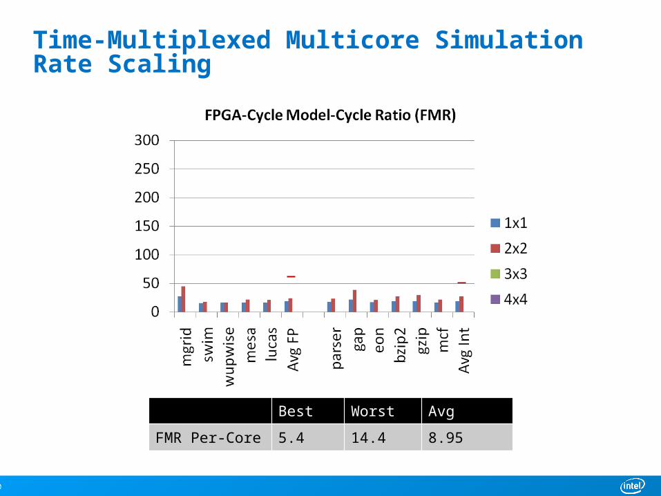
Time-Multiplexed Multicore Simulation Rate Scaling

Best Worst Avg

FMR Per-Core 5.4 14.4 8.95

31

Time-Multiplexed Multicore Simulation Rate Scaling

Best Worst Avg

FMR Per-Core 8.5 13.5 11.6

32

Time-Multiplexed Multicore Simulation Rate Scaling

Best Worst Avg

FMR Per-Core 8.45 19.8 11.5

33

Takeaways

The Latency-Insensitive approach provides a unified approach to interesting tradeoffs

Serialization: Leverage FPGA-efficient circuits at the cost of FMR

• A-Port-based synchronization can amortize cost by giving dynamic average

• Especially if long events are rare

Time-Multiplexing: Reuse datapaths and only duplicate state

• A-Port based approach means not all modules are fully utilized

• Increased utilization means that performance degradation is sublinear

• Time-multiplexing the on-chip network requires permutations

34

Next Steps

Here we were able to push one FPGA to its limits

What if we want to scale farther?

Next, we’ll explore how latency-Insensitivity can help us scale to multiple FPGAs with better performance than traditional techniques

Also how we can increase designer productivity by abstracting platform

36

Resynchronizing Ports

Modules follow modified scheme:• If any incoming port is heavy, or any outgoing port is light, simulate next

cycle (when ready)• Result: balanced w/o centralized coordination

Argument: • Modules farthest ahead in time will never proceed• Ports in (out) of this set will be light (resp. heavy)

– Therefore those modules will try to proceed, but may not be able to

• There’s also a set farthest behind in time– Always able to proceed– Since graph is connected, simulating only enables modules, makes progress

towards quiescence

37

Other Topologies

Tree

Butterfly

[1 , 1 , 1 , 0 , 0 , 0 , 0 ] [1 , 1 , 1 , 0 , 0 , 0 , 0 ][0 , 0 , 0 , 1 , 1 , 1 , 1 ]

[2 , 0 , 1 , 0 , 1 , 0 , 1 ] [0 , 1 , 2 , 1 , 2 , 1 , 2 ]

P hys ica lR ou ter

[0 , 0 , 0 , 1 , 1 , 1 , 1 ]

R ou ter0

R ou ter2

R ou ter1

R ou ter6

R ou ter5

R ou ter4

R ou ter3

[0 , 0 , 1 , 1 , 0 , 1 , 0 , 1 , 2 , 2 , 2 , 2 ] [1 , 1 , 2 , 2 , 1 , 2 , 1 , 2 , 0 , 0 , 0 , 0 ]

[0 , 1 , 0 , 1 , 0 , 1 , 0 , 1 ]

[0 , 1 , 0 , 1 , 0 , 1 , 0 , 1 ]

[2 , 2 , 2 , 2 , 0 , 0 , 1 , 1 , 0 , 1 , 0 , 1 ]

F rom P hys ica l C ore

To P hys ica l C ore

[2 , 2 , 2 , 2 , 0 , 0 , 1 , 1 , 0 , 1 , 0 , 1 ]

P hys ica lR ou ter

To C ore 0

To C ore 1

R ou ter8

To C ore 2

To C ore 3

R ou ter9

To C ore 4

To C ore 5

R ou ter10

To C ore 6

To C ore 7

R ou ter11

R ou ter4

R ou ter5

R ou ter6

R ou ter7

R ou ter0

R ou ter1

R ou ter2

R ou ter3

F rom C ore 0

F rom C ore 1

F rom C ore 2

F rom C ore 3

F rom C ore 4

F rom C ore 5

F rom C ore 6

F rom C ore 7

38

Generalizing OCN Permutations

•Represent model as Directed Graph G=(M,P)•Label modules M with simulation order: 0..(N-1)

•Partition ports into sets P0..Pm where:– No two ports in a set Pm share a source– No two ports in a set Pm share a destination

• Transform each Pm into a permutation σm

– Forall {s, d} in Pm, σm(s) = d– Holes in range represent “don’t cares”– Always send NoMessage on those steps

• Time-Multiplex module as usual– Associate each σm with a physical port

39

Example: Arbitrary Network

0

4

3

2

15

A

1032

543210

10

543210

14

543210

C

0

2

1

B

(1, 0)(3, 1)

P0

P1

P2

(5, 1)

(1, 2)(2, 3)(4, 0)

(0, 4)(4, 1)

40

Results: Multicore Simulation Rate

FMR Simulation Rate

Min Max Avg Min Max Avg

Overall 16 218 80 160 KHz 3.2 MHz 625 KHz

Per-Core 5 27 11 1.84 9.5 MHz 4.54 MHz

• Must simulate multiple cores to get full benefit of time-multiplexed pipelines

• Functional cache-pressure rate-limiting factor