1 

 

Has the introduction of IFRS improved accounting quality? A

comparative study of five countries

Corresponding author: Andreas Jansson, Assistant Professor, PhD, School of Business and Economics, Linnaeus University, Växjö, Sweden

e-mail: andreas.jansson@lnu.se

Phone: +46-470-708230

Fax: +46-772288000

Micael Jönsson, Research Assistant, School of Business and Economics, Linnaeus University, Växjö, Sweden

Christopher von Koch, Assistant Professor, PhD, School of Business and Economics, Linnaeus University, Växjö, Sweden

2 

 

Has the introduction of IFRS improved accounting quality? A comparative study of five

countries

Abstract

This paper investigates whether the implementation of International Financial Reporting

Standards (IFRS) has increased accounting quality. Previous research has primarily explored

the effects of IFRS on accounting quality as measured through the use of value relevance,

timely loss recognition and earnings management. In contrast, this paper employs a measure

of accounting quality that is based on the use of accounting information, namely, the

performance of financial analysts. The sample encompasses nearly 2,500 publicly traded

firms, all followed by analysts, from 1996-2009. The sample covers five European countries

(Sweden, Netherlands, France, Germany and the United Kingdom (the UK)), each with

different legal and accounting traditions. We use quantile regressions to estimate the impact

of IFRS while simultaneously considering that most prediction errors are small and are most

likely random and unaffected by the accounting standard being followed. Our results suggest

that IFRS have had no effect on analysts’ average ability to accurately forecast firms’

earnings per share. In all countries except the UK, IFRS have led to higher consistency in

analyst forecasts. The impact of IFRS is not more pronounced in firms that are more affected

by their asset measurement methods. The results suggest that in countries where prior GAAP

differ from IFRS, IFRS may have the effect of presenting more consistent but not more

accurate pictures of firms for analysts.

Keywords: IFRS, accounting quality, analyst forecasts, comparative study

3 

 

1. Introduction

With regulation EC No 1606/2002, the European Union (EU) decided that all publicly traded

companies “shall prepare their consolidated accounts in conformity with the international

accounting standards [IAS]” (EU, 2002: Article 4) for each financial year beginning on or

after 1 January 2005. More specifically, this requirement means that these companies must

apply IAS, International Financial Reporting Standards (IFRS) and Standing Interpretations

Committee/International Financial Reporting Standards Interpretation Committee

(SIC/IFRSIC) interpretations issued by the International Accounting Standards Board (IASB).

This requirement most likely constitutes the single most significant change in accounting

standards to have ever occurred in Europe and is popularly referred to as the introduction of

IFRS (for a comprehensive description of the implementation of IFRS, see, for example,

Armstrong et al. 2010). In this paper, we empirically examine the impact of the introduction

of IFRS on the accuracy and dispersion of financial analysts’ forecasts in five EU countries.

The past decade has seen a large amount of empirical research regarding what constitutes

high-quality accounting (see Soderstrom and Sun, 2007 for a review). For many European

countries, the introduction of IFRS has entailed substantial changes in accounting methods,

and this change has prompted a major ‘natural’ opportunity to examine factors thought to

affect accounting quality. Consistently, academics around the world are now extensively

studying the effects of IFRS on accounting quality (see, for example, Armstrong et al., 2010;

Ball, 2006; Barth et al., 2008; Bartov et al., 2005; Byard et al., 2011; Daske and Gebhardt,

2006; Daske et al., 2008; Ding et al., 2007; Hung and Subramanyam, 2007; Jeanjean and

Stolowy, 2008; Jiao et al., 2012). Results from these studies are mixed. On the one hand,

IFRS appear to have a positive effect on accounting quality, but the results are contingent on

country- or firm-specific characteristics. In general, IFRS require more extensive and

4 

 

sophisticated disclosures than were afforded by prior local standards, and this requirement

may have a positive influence on the quality of financial reports. On the other hand, certain

aspects of IFRS, such as the greater flexibility in choice of accounting methods that it offers

in comparison with some EU countries’ previous local standards, may be negatively affecting

accounting quality (e.g., Ormrod and Taylor, 2004).

Previous research has commonly used earnings management, timely loss recognition and

value relevance as indicators of accounting quality (cf. Barth et al., 2008), although metrics

such as quality indices and appropriateness also appear. All of these metrics fail to directly

capture the usefulness of the information to accounting users. In this paper, we approach the

effect of IFRS on accounting quality from a different angle by determining whether the

introduction of IFRS has allowed users of accounting information to make better predictions

regarding firm performance. More specifically, we examine whether the introduction of IFRS

has allowed financial analysts to formulate better forecasts of firm performance. This decision

usefulness dimension of accounting quality is in line with a purpose of accounting that is

stressed in the conceptual framework of the IASB, which states that

The objective of general purpose financial reporting is to provide financial

information about the reporting entity that is useful to existing and potential

investors, lenders and other creditors in making decisions about providing

resources to the entity. Those decisions involve buying, selling or holding

equity and debt instruments, and providing or settling loans and other forms of

credit (IASB, 2010: OB2).

Financial analysts are often argued to fulfill an important function in financial markets by

reducing the information asymmetry between firms and investors through their intermediary

5 

 

role (Lang and Lundholm, 1996). However, financial analysts’ ability to perform their task is

contingent on the information shared between themselves and the firm not being too

asymmetrical (cf. Krishnaswami and Subramaniam, 1999). Available evidence suggests that

financial analysts rely extensively on accounting information to make forecasts (Block, 1999;

Roger and Grant, 1997); analysts are also considered to be sophisticated users of accounting

information (e.g., Schipper, 1991). Prior research has focused primarily on the role of

voluntary disclosure in reducing this information asymmetry (Barry and Brown, 1985;

Glosten and Milgrom, 1985; Lang and Lundholm, 1996; Merton, 1987), but the introduction

of IFRS also allows for the exploration of impacts that mandatory financial accounting may

have on analysts’ ability to reduce information asymmetry. Higher quality financial

accounting could be expected to allow extensive users of accounting data to formulate higher

quality assessments of firms, leading to less overall information asymmetry.

Because the impact of IFRS on accounting quality appears to vary among countries, it is

unlikely to have the same effects on analysts’ performance in all countries where it is

introduced. Barth et al. (2008), Byard et al. (2011), Daske et al. (2008) and Preiato et al.

(2010), for example, suggest that the enforcement of accounting standards, which can vary

among countries (La Porta et al., 1998), is pivotal for the realization of quality increases

through the introduction of IFRS. Therefore, in this study, we examine the impact of IFRS on

accounting quality in five EU countries: Sweden, the UK, Germany, France and the

Netherlands. These countries have regulatory systems with different origins and with varying

enforcement strength (La Porta et al., 1998; Preiato et al., 2010), which is reflected in their

varying financial accounting traditions (Nobes, 1983).

Our paper is related to a number of previous studies. Ashbaugh and Pincus (2001), who

examined 80 non-US firms that voluntarily adopted IAS during the 1990-93 period, found

6 

 

that analysts’ forecast accuracy increases after firms adopt IAS and that the convergence in

firms’ accounting policies that is achieved by adopting IAS is positively associated with a

reduction in analysts’ forecast errors. Some early studies have examined the effects of

mandatory IFRS adoption on analysts’ performance. For example, Byard et al. (2011) found

that forecast errors and forecast dispersion decrease, but only in countries with both strong

enforcement regimes and domestic accounting standards that differ significantly from IFRS.

Similar conclusions are suggested in Horton et al. (2012) and Preiato et al. (2010) who

demonstrate that IFRS can have a positive impact on forecast accuracy if enforcement is

strong. Consistent with this notion, Tan et al. (2011) demonstrate that the accuracy of foreign

financial analysts’ forecasts increases when IFRS are implemented, particularly if the

difference between previous local Generally Accepted Accounting Principles (GAAP) and

IFRS is significant; however, domestic analysts’ accuracy is not affected by IFRS. Beuselinck

et al. (2010) and Yang (2010) examine the impact of IFRS on private and public information

precision. They found a positive association between IFRS and public information precision,

which is consistent with an increase in accounting quality. However, Beuselinck et al. (2010)

suggest that the effect is more significant in countries in which IFRS entail a significant

change, whereas Yang (2010) suggests that the improvement is more significant in countries

that already had high-level disclosure standards. Glaum et al. (forthcoming), who examined

the impact of IFRS on analysts following Germans firms, separated the effect between

improved disclosure and other changes in the firms’ information environments. They found

that improved disclosure had a modest and positive effect on analysts’ accuracy but suggest

that improvements in the quality of earnings, improvements in firms’ investor relations and

changes in analyst behavior have contributed more to the improvement of analyst accuracy.

Overall, the literature suggests that IFRS have a positive but not uniform impact.

7 

 

Our results, which are based on a sample comprising 2,447 public companies from 5 EU

countries during the period of 1996-2009, suggest that IFRS have no impact on forecast

accuracy but appear to reduce forecast dispersion. However, the effect of this dispersion is

small. In fact, the effect on dispersion is nonexistent for the UK, the country that exhibits the

smallest difference between previous GAAP and IFRS. Furthermore, the effect is only visible

for the median part of the distribution of forecast dispersions; for large as well as small

dispersions, there is no significant effect. Overall, our results suggest that IFRS appear to

provide a more consistent but not more accurate picture of firms, a conclusion that is also

strengthened by the finding that these effects appear to not be driven by IFRS’ ability to better

represent the underlying economic value of a firm.

Four aspects of our approach distinguish our study from prior empirical studies on the effects

of IFRS. First, we contribute to the literature using a sample of forecast accuracy and forecast

dispersion that encompasses an extensive time period. As Preiato et al. (2010) suggest, analyst

performance differs significantly over time for reasons that are unrelated to accounting

regulation. It is therefore important to include both periods of generally strong and periods of

generally poor analyst performance from both the pre and post IFRS adoption period to better

isolate the effects of IFRS. Second, to analyze our dataset, we use an estimation technique – a

quantile regression model – that is robust to the problem of skewness. As Yang (2010) argues,

skewness, which can bias estimates, is a serious problem with this type of data. Yang (2010)

suggests that a median regression model could remedy this problem. The use of a median

regression model allows us to estimate coefficients without manipulating the dataset, which

would not be possible with an OLS regression model of estimation. Third, our estimation

technique also allows us to predict the effect of independent variables on different magnitudes

of forecast errors and forecast dispersions. This approach allows us to detect the effect of

8 

 

IFRS on large and small errors without assuming the same impact across the entire

distribution. It is reasonable to assume that the impact of IFRS is not uniform in this respect

because most small errors or dispersions are likely to be random and therefore impossible to

eliminate through the use of improved accounting. Fourth, we use a different proxy for the

firm-level impact of IFRS. Although prior studies have used industry (e.g., Beuselinck et al.,

2010) and differences in reported earnings in reconciliation accounts (e.g., Horton et al.,

2012) as proxies for the firm-level impact of IFRS, we use an accounting figure that is highly

affected by IFRS as a proxy: intangible assets. Intangible assets, which are difficult for an

analyst to valuate because they are typically unique, are regularly valued at fair value (i.e.,

market value or a proxy thereof) in IFRS; traditionally, these assets have been valued at

historical cost. This method allows us to generate new evidence on what aspect of IFRS might

affect analyst performance.

Our results have a number of theoretical and practical implications. The results indicate the

need to distinguish between two aspects of accounting quality: how it affects users’ accuracy

and how it affects users’ consistency. Accounting quality measures should be developed to

accommodate this distinction. The fact that IFRS primarily affect consistency implies that

fair-value appraisals of asset values are used by analysts when predicting firm performance

and that IFRS have therefore created a more level playing field despite their lack of a

significant effect on predictive value.

2. Hypotheses development

2.1 IFRS and forecast accuracy

Our approach relies on the assumption that higher quality accounting will be reflected in

higher quality forecasts by financial analysts. Revsine et al. (2004) and Schipper (1991) argue

9 

 

that analysts are considered to be among the most important and influential users of financial

reports and among the most important information intermediaries between firms and

investors. Considering their information-processing ability and access to resources, analysts

are typically viewed as sophisticated users of accounting information and as being less likely

(than naïve investors) to misunderstand the implications of such information (e.g., Schipper,

1991). Therefore, if financial analysts receive access to higher quality financial reports, they

should be able to make better predictions, measured as higher forecast accuracy.

Lang and Lundholm (1996) provide evidence of the relationship between disclosure and

decreased information asymmetry. Firms with more informative disclosure policies enjoy a

larger analyst following, more accurate earnings forecasts, less dispersion among forecasts,

and less volatility in forecast revisions. Firms that provide firm-specific information, in

particular, are associated with more accurate earnings forecasts and less forecast dispersion.

Soderstrom and Sun (2007) argue that the accounting standard being followed affects

accounting quality. This relationship implies that the introduction of a new accounting

standard should affect the accounting quality of a firm on the margin. The introduction of

IFRS has necessitated an accounting standard change for most EU-member countries and, in

turn, this change should be reflected in accounting quality. In general, the change to IFRS has

entailed a shift toward more valuation of assets according to fair value instead of historical

cost. This shift should mean that IFRS provide a better picture of the underlying economic

value for firms in the EU because changes in the value of assets generally will be accounted

for on a regular basis. However, at the same time, fair value accounting is likely to provide

managers with more discretion in accounting, which might diminish the quality of accounting

because of increased earnings management (Ormrod and Taylor, 2004).

10 

 

Empirical research (e.g., Armstrong et al., 2010; Ball, 2006; Barth et al., 2008; Bartov et al.,

2005; Byard et al., 2011; Daske and Gebhardt, 2006; Daske et al., 2008; Ding et al., 2007;

Hung and Subramanyam, 2007; Jeanjean and Stolowy, 2008) has attempted to compare the

quality – measured primarily in terms of value relevance, earnings management and timely

loss recognition – of IFRS and that of previous standards. The overall quality assessment is

not conclusive (cf. Soderstrom and Sun, 2007), perhaps because of the two opposing effects

of IFRS (Ormrod and Taylor, 2004). Nevertheless, in terms of supporting high-quality

decision making by financial analysts, it is reasonable to assume that a better representation of

underlying economic value will outweigh the negative effects of an increase in management

discretion. Thus, our first hypothesis is as follows:

H1: The introduction of IFRS increases the accuracy of analysts’ earnings forecasts

2.2 IFRS and forecast dispersion

Forecast dispersion (measured as the standard deviation in analysts’ forecasts), which is an

indication of the extent of analysts’ disagreement regarding a firm’s upcoming earnings, can

be used as a proxy for investor uncertainty prior to the release of key information (Ramnath et

al., 2008).According to Krishnaswami and Subramaniam (1999), this dispersion is a measure

of information asymmetry. They claim that when information asymmetry between a firm and

its market is high, it is difficult for the market to evaluate or predict the firm’s performance.

This difficulty increases firm uncertainty.

We assume that higher quality accounting will decrease information asymmetry and therefore

decrease firm uncertainty, leading to less forecast dispersion. With their stronger orientation

toward fair value accounting, IFRS are likely to provide a better representation of a firm’s

underlying economic value and should therefore decrease information asymmetry. However,

11 

 

increased opportunities for managerial discretion could create a degree of uncertainty. The

effect of IFRS on forecast dispersion may also depend on whether analysts use more public or

private information (Heflin et al., 2003; Irani and Karamanou, 2003). If public information is

the primary source used, there should be less dispersion because public information is

available to all. However, if analysts seek to gain advantage by gathering private information

in response to an increase in public information, policies for the improvement of accounting

information may increase dispersion. It could also be the case that analysts choose to ‘herd’

when earnings are more uncertain, leading to less forecast dispersion for firms with less

predictable earnings (Ramnath et al., 2008). Using the BKLS model, Yang (2010) empirically

tests whether analysts use more public or private information after IFRS adoption in 18

countries. Yang concludes that both public and private information increase after mandatory

IFRS adoption and that the overall effect is a decrease in forecast dispersion among analysts.

Interestingly, public and private information increase more in common law countries than in

civil law countries, indicating that dispersion can increase in some countries while decreasing

in others.

Because available evidence suggests that financial analysts use financial reports as a primary

source (Block, 1999; Roger and Grant, 1997) of firm information and because it is likely that

a better representation of the underlying economic value will outweigh the negative effects of

an increase in management discretion, our second hypothesis is as follows:

H2: The introduction of IFRS reduces the dispersion of analysts’ earnings forecasts

2.3 The relative impact of IFRS

The last decade has seen the emergence of considerable research discussing the influence of

legal and institutional settings on accounting quality (e.g., Byard et al., 2011; Soderstrom and

12 

 

Sun, 2007). In several cases, the research is based on the assumption that these settings have a

significant impact on accounting quality, which, in turn, affects analysts’ ability to make

accurate forecasts. Other studies have also emphasized firm-specific characteristics, as well as

the importance of reporting firms’ incentives as salient factors in the success of IFRS. Byard

et al. (2011) and Jeanjean and Stolowy (2008), for example, stress the importance of firms’

reporting incentives, which are influenced by legal institutions, various market forces, firms’

operating characteristics and the like. In line with Zeff (2007), it is therefore reasonable to

assume that country-specific differences such as business and financial culture, accounting

culture, auditing culture and regulatory culture are likely to affect the success of IFRS

implementation.

We should therefore expect the introduction of IFRS to have different effects on accounting

quality in different legal and institutional settings. For instance, one variable aspect is the

strength of accounting standard enforcement (Preiato et al., 2010), which influences

managerial discretion. Studies by Francis et al. (2003) and Hope (2003), among others, found

that common law countries (i.e., the UK and Ireland) have stronger enforcement mechanisms

than code law countries (i.e., the rest of the EU). The international accounting literature also

indicates that accounting quality is higher in countries with a common law origin (Ali and

Hwang, 2000; Ball et al., 2000; Leuz et al., 2003), and enforcement mechanisms appear to

influence the expected quality of financial reporting under IFRS (Ball et al., 2000; Ball, 2006;

Barth et al., 2008; Byard et al., 2011; Dao, 2005; Daske et al., 2008). Barth et al. (2008)

conclude that the potential benefits of the introduction of IFRS are difficult to attain without

the existence of effective enforcement mechanisms (cf. Byard et al., 2011; Preiato et al.,

2010).

13 

 

Another important factor is the quality of the accounting standard previously used in a given

country. If the standard was of low quality, the positive effects of changing to a standard that

better reflects a firm’s underlying economic value would be expected to be more significant

(Byard et al., 2011). The magnitude of differences between IFRS and the local GAAP that

they have replaced varies considerably (Bae et al., 2008; Nobes, 1983), and it is therefore

reasonable to expect IFRS’ effect on analyst performance to vary among countries. Thus, our

third set of hypotheses is as follows:

H3a: The larger the difference between IFRS and the previous GAAP, the more the

introduction of IFRS increases forecast accuracy

H3b: The stronger the enforcement of accounting standards, the more the introduction of

IFRS increases forecast accuracy

H4a: The larger the difference between IFRS and the previous GAAP, the more the

introduction of IFRS decreases forecast dispersion

H4b: The stronger the enforcement of accounting standards, the more the introduction of

IFRS decreases forecast dispersion

2.4 The moderating effect of intangible assets

IFRS imply a higher degree of fair value accounting. In particular, IFRS systematically

employ fair value accounting for classes of assets such as intangible assets, financial

instruments, investment property and biological assets. Therefore, the potential improvement

triggered by IFRS in terms of the correspondence between firms’ accounting and underlying

economic value is likely to be more sizeable for firms with a higher proportion of such assets.

In the absence of fair value accounting data, intangible assets are particularly difficult for

14 

 

analysts to value because they are often unique and, as such, lack official market values.

Therefore, it is reasonable to assume that the higher the proportion of a firm’s intangible

assets, the more analysts’ forecast accuracy will improve and forecast dispersion diminish

following the introduction of IFRS. Our fifth and sixth hypotheses are therefore as follows:

H5: The higher the proportion of intangible assets, the more the introduction of IFRS

increases the accuracy of analysts’ earnings forecasts

H6: The higher the proportion of intangible assets, the more the introduction of IFRS reduces

the dispersion of analysts’ earnings forecasts

3. Method and sample

3.1 Sample

Our sample consists of 2,447 publicly traded companies from five European countries. The

countries were chosen primarily because of differences in the countries’ accounting histories

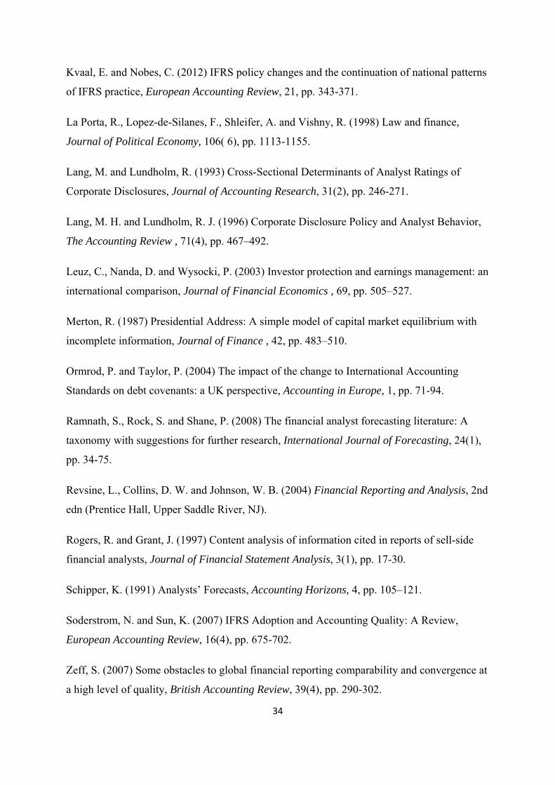
(Nobes, 1983). Our third and fourth hypotheses identify the two relevant dimensions as being

the difference between previous GAAP and IFRS and the enforcement of accounting

standards. Table 1 reports measures of these two dimensions pertaining to the five countries in

the sample.

-----------------------------------------------------------------------------------

Insert Table 1 about here

--------------------------------------------------------------------------------------

15 

 

The measure of difference between previous GAAP and IFRS (henceforth GAAP-difference)

is provided by Bae et al. (2008), who report an index measuring conformity with IAS

consisting of 21 specific items in 2001. The higher the number, the larger the difference is, the

maximum value being 21. The measure is likely to overstate the change resulting from

mandatory IFRS adoption because many local standard setters began to harmonize local

GAAP with IAS before the mandatory adoption period. However, the measure is likely to

capture the difference between IFRS and the more long-term, prior accounting tradition in

each country, which, according to Kvaal and Nobes (2012), have a persistent influence on

accounting despite IFRS adoption. We also report a measure of accounting standard

enforcement developed by Preiato et al. (2010), which is based on 19 items and a scale

ranging from 0 to 27, capturing effects of the strength of the audit function and the accounting

enforcement body, respectively. The table reports the measure for the year 2005, when IFRS

were made mandatory in our sample countries.

Our sample countries display variation on the dimensions of GAAP-difference and

enforcement. The UK and the Netherlands exhibit the smallest GAAP-difference, whereas

France, Germany and Sweden display larger differences. The UK is regarded as having strong

enforcement. According to Preiato et al. (2010), Sweden and the Netherlands have relatively

weak enforcement, whereas France and Germany have stronger enforcement.

Together, these results suggest four clusters: (i) France and Germany, which display both a

relatively significant GAAP-difference and relatively strong enforcement; (ii) the UK, which

displays a negligible GAAP-difference but strong enforcement; (iii) Sweden, which exhibits a

sizeable GAAP-difference and weak enforcement; and (iv) the Netherlands, which displays a

small GAAP-difference and weak enforcement. This clustering would suggest that based on

hypotheses three and four, we could expect the strongest impact on analyst performance to

16 

 

occur in France and Germany. Conversely, the effect could be expected to be negligible in the

Netherlands. Sweden and the UK appear to be opposites. Therefore, if GAAP-difference is

more important to IFRS impact than enforcement, we would expect the effect on analyst

performance to be more pronounced in Sweden than in the UK and vice versa.

3.2 Variables and descriptive statistics

Analysts’ performance is usually measured in the financial literature in terms of forecast

accuracy and/or the correctness of stock recommendation or price target, depending on how

the final output is viewed. Schipper (1991) discusses the reasonable belief that analysts’

earnings forecasts should relate to their stock recommendations, which suggests that forecasts

and valuation estimates (relative to current price) should be positively related to stock

recommendations. However, research into this area does not support these conjectures.

Bradshaw (2004) demonstrates that recommendations and valuation estimates in the US are

either insignificantly or negatively related, depending on the specification. EPS predictions

are likely to suffer from less bias and better reflect analysts’ use of accounting information

and, therefore, accounting quality.

To make a forecast, an analyst processes much information from a firm; the degree of

accuracy is therefore highly related to the level of informational asymmetry between the

analyst and the firm. Accordingly, forecast accuracy is selected as our first performance

variable. Because the literature also suggests that forecast dispersion could be viewed as a

measure of information asymmetry (Krshnaswami and Subramaniam 1999), forecast

dispersion is our second performance variable.

In accordance with Lang and Lundholm (1996), the first dependent variable, forecast

accuracy, is calculated as the negative of the absolute value of the actual earnings minus the

17 

 

analyst’s earnings forecast, scaled by the stock price at the beginning of the year, and

forecasted EPSt is the mean analyst forecast of the earning per share during period t.

year fiscal theof beginning at the priceStock Accuracy Forecast tt EPSForecastedEPSActual −−=

Forecast accuracy is defined as the negative of the scaled absolute forecast error. In other

words, more accurate forecasts are represented by higher (less negative) values, i.e., lower

forecast error, with zero representing a perfect forecast. Analysts usually forecast the earnings

per share (EPS) of a particular fiscal year several times before the actual figures are released.

The frequency of the forecasts differs in accordance with the analyst. The Institutional

Brokers’ Estimate System (I/B/E/S) collects forecast data from individual analysts around the

world once a month and uses those data to calculate statistics such as the mean, median, and

standard deviation. Only the final estimates of the analysts are included in the monthly

calculation. Thus, the I/B/E/S database provides calculated statistics of analysts’ EPS

forecasts once a month. In this study, we utilize the general methodology for collecting

forecast data (see, for example, Lang and Lundholm, 1996) using the final calculated mean of

an analyst’s EPS forecasts before the first quarterly EPS report is released. For example, for a

firm with a fiscal yearend of December 31, 2009, we use the mean forecast calculated in

March 2009 as the forecast data for the actual EPS on December 31, 2009.

The second dependent variable, forecast dispersion, is the inter-analyst standard deviation of

forecasts, scaled by the stock price at the beginning of the year, also in line with Lang and

Lundholm (1996). Standard deviations are always positive numbers, but we have changed the

sign so that the logic in use for the scale of forecast dispersion is the same as that in use for

forecast accuracy, i.e. so that a lower (more negative) forecast dispersion represents a higher

standard deviation.

18 

 

Because the forecast measures are scaled with stock price, cross-company comparisons are

possible. To test our hypotheses, we use two test variables, ‘accounting standard followed’

and ‘interaction term,’ which is the interaction between the standard followed and the

proportion of intangible assets, and six control variables. Accounting standard followed is a

dummy variable for which 1 is used for IFRS and 0 is used for every other accounting

standard. This variable is a firm-level variable, which means that early IFRS adopters are

identified as IFRS users even though this usage is not mandatory. The variable is set to 1 one

year after a firm’s implementation of IFRS because analysts could not have based their

adoption-year predictions on IFRS accounting, as the EPS predictions we use were formulated

before the first IFRS-based quarterly report. We obtain the interaction term by multiplying the

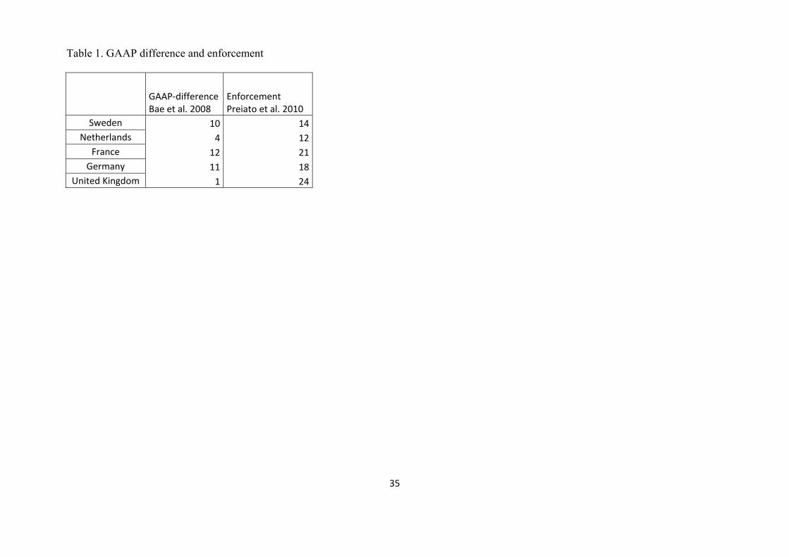
dummy variable by the proportion of intangible assets to total assets. The six control variables

(see Table 2), selected on the basis of prior research into factors that normally affect analysts’

performance (Lang and Lundholm 1996), are as follows: number of analysts, market value,

trading volume, earnings surprise, profit/loss, and standard deviation of return on equity (std

ROE).

-----------------------------------------------------------------------------------

Insert Table 2 about here

--------------------------------------------------------------------------------------

The number of analysts is determined by simply a count of those following the company and

providing earnings forecast, again in line with Lang and Lundholm (1996). We control for

firm size using market value and trading volume. Firm size is used in the literature as a proxy

for several factors. Size should reflect information availability and therefore be positively

related to forecast accuracy. Brennan and Hughes (1991) also found empirical evidence

19 

 

between firm size and analysts following a firm, and Lang and Lundholm (1993) found that

firm size and performance variability likely correlate with disclosure policy. Market value is

measured as the company’s market value at the beginning of the fiscal year and is commonly

used to control for size. However, we also utilize trading volume as a control for size because

it may be more indicative of the number of analysts following a firm, as analysts are often

paid indirectly through trading activity. Trading volume refers to the company’s absolute

daily trading volume during the first month of the fiscal year. Earnings surprise, which is the

variation in a firm’s results from one year to another, is calculated as the absolute value of the

year’s earnings per share minus the previous year’s earnings per share, scaled by the share

price at the beginning of the fiscal year. EPSt is the earnings per share during period t (of a

given year), and EPSt-1 is the earnings per share during period t-1 (the previous year).

year fiscal theof beginning at the priceStock SurpriseEarnings 1−−= tt EPSEPS

According to Lang and Lundholm (1996), earnings surprise controls for the likely effect that

major events, such as a firm's introduction of a new product, have on forecasts. In these

circumstances, realized earnings are most apt to deviate from expected earnings, and it is

likely that analysts will not be able to make accurate forecasts.

Hope (2003) suggests that it is much more difficult to predict future earnings for firms with

negative earnings. We therefore use a control variable, loss, a dummy variable that has a

value of 1 if the company reported a loss and 0 otherwise. King et al. (1990) found that the

number of analysts following firms is likely to be related to variations in return. Fewer

analysts follow firms that experience significant fluctuations in profitability. In other words, a

negative relationship exists between the number of analysts and variations in profitability.

20 

 

Thus, standard deviation of return on equity is the final control variable in our regressions,

and it is measured as the company’s return on equity over the previous three years.

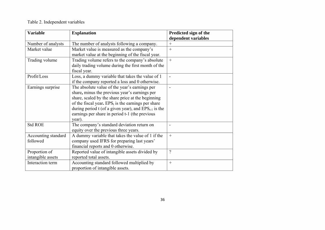
Table 3 contains descriptive statistics for the sample. Within each country, we select all

publicly traded companies that were followed by analysts. We do not attempt to follow

individual analysts because we assume that the ability to predict values for a specific firm

improves over time and therefore might bias the results. From this population, we then

extracted those companies with at least one year of both IFRS reporting and non-IFRS

reporting. Persuaded by Byard et al.’s (2011) argument regarding the necessity of examining

the impact of IFRS on analysts’ forecasts over a longer time period, we chose the period of

1996-2009. However, it should be noted that because some companies existed during this

entire time period and others for only a couple of years, our sample is an unbalanced panel

data set. From our full sample, we obtained 17,449 valid observations of forecast accuracy

and 15,003 valid observations of forecast dispersion. We are missing observations of forecast

dispersion because those firms followed by only one analyst cannot display forecast

dispersion. Forecast accuracy is calculated as a mean of all analysts’ predictions for a specific

firm (the number of analysts ranges from 1 to 49). As Table 3 shows, the mean forecast error

for the full sample is approximately 6.3 percent, with the worst analyst performance occurring

in Germany and the best in the UK. The mean forecast dispersion is highest in Germany and

lowest in the UK.

-----------------------------------------------------------------------------------

Insert Table 3 about here

--------------------------------------------------------------------------------------

21 

 

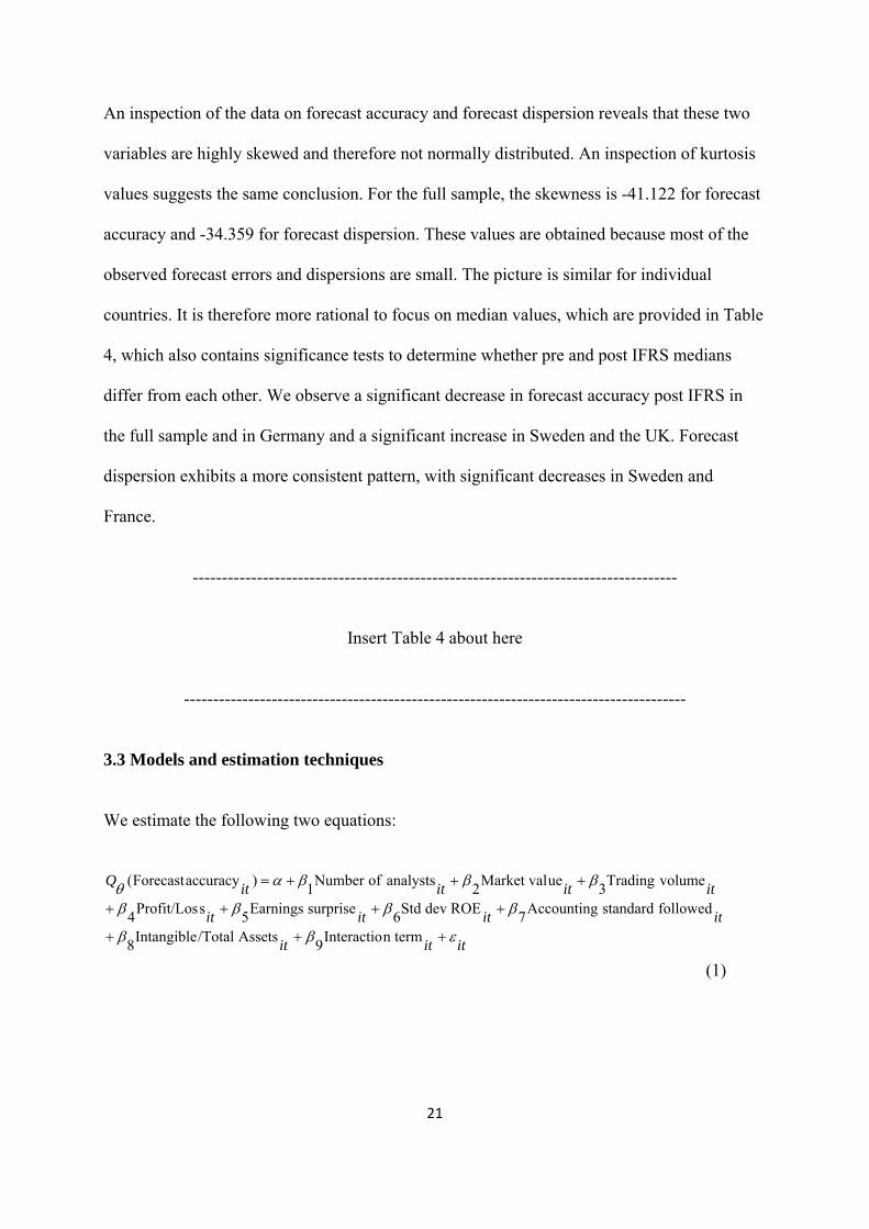
An inspection of the data on forecast accuracy and forecast dispersion reveals that these two

variables are highly skewed and therefore not normally distributed. An inspection of kurtosis

values suggests the same conclusion. For the full sample, the skewness is -41.122 for forecast

accuracy and -34.359 for forecast dispersion. These values are obtained because most of the

observed forecast errors and dispersions are small. The picture is similar for individual

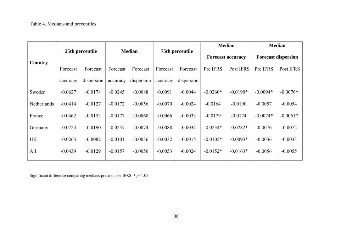
countries. It is therefore more rational to focus on median values, which are provided in Table

4, which also contains significance tests to determine whether pre and post IFRS medians

differ from each other. We observe a significant decrease in forecast accuracy post IFRS in

the full sample and in Germany and a significant increase in Sweden and the UK. Forecast

dispersion exhibits a more consistent pattern, with significant decreases in Sweden and

France.

-----------------------------------------------------------------------------------

Insert Table 4 about here

--------------------------------------------------------------------------------------

3.3 Models and estimation techniques

We estimate the following two equations:

ititit

itititit

ititititQ

εββ

ββββ

βββαθ

+++

++++

+++=

n termInteractio9 Assets /TotalIntangible8

followed standard Accounting7ROE dev Std6surprise Earnings5sProfit/Los4

volumeTrading3ueMarket val2analysts ofNumber 1)accuracyForecast(

(1)

22 

 

ititit

itititit

ititititQ

εββ

ββββ

βββαθ

+++

++++

+++=

n termInteractio9assets /TotalIntangible8

followed standard Accounting7ROE dev Std6surprise Earnings5sProfit/Los4

volumeTrading3ueMarket val2analysts ofNumber 1)dispersionForecast (

(2)

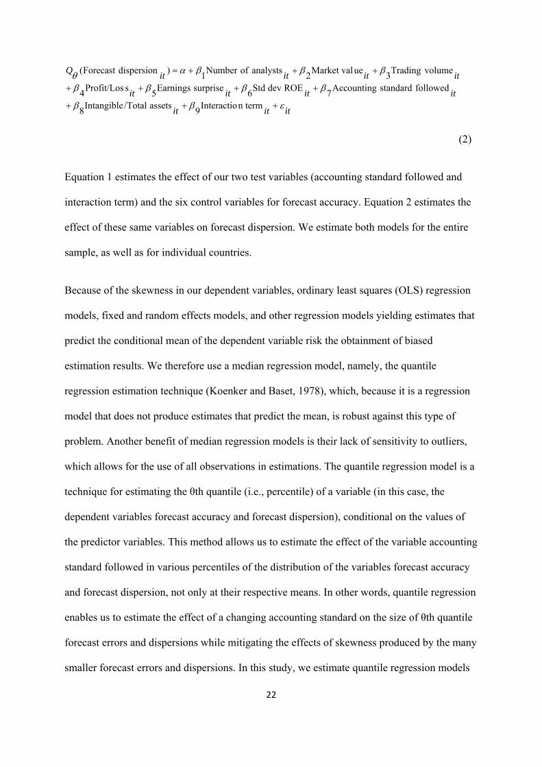
Equation 1 estimates the effect of our two test variables (accounting standard followed and

interaction term) and the six control variables for forecast accuracy. Equation 2 estimates the

effect of these same variables on forecast dispersion. We estimate both models for the entire

sample, as well as for individual countries.

Because of the skewness in our dependent variables, ordinary least squares (OLS) regression

models, fixed and random effects models, and other regression models yielding estimates that

predict the conditional mean of the dependent variable risk the obtainment of biased

estimation results. We therefore use a median regression model, namely, the quantile

regression estimation technique (Koenker and Baset, 1978), which, because it is a regression

model that does not produce estimates that predict the mean, is robust against this type of

problem. Another benefit of median regression models is their lack of sensitivity to outliers,

which allows for the use of all observations in estimations. The quantile regression model is a

technique for estimating the θth quantile (i.e., percentile) of a variable (in this case, the

dependent variables forecast accuracy and forecast dispersion), conditional on the values of

the predictor variables. This method allows us to estimate the effect of the variable accounting

standard followed in various percentiles of the distribution of the variables forecast accuracy

and forecast dispersion, not only at their respective means. In other words, quantile regression

enables us to estimate the effect of a changing accounting standard on the size of θth quantile

forecast errors and dispersions while mitigating the effects of skewness produced by the many

smaller forecast errors and dispersions. In this study, we estimate quantile regression models

23 

 

predicting the 10th, 50th (i.e., the median) and 90th percentile for the full sample, as well as

for individual countries. Thus, when predicting the 10th percentile, we study the effect of

IFRS on only the largest forecast errors or highest dispersions. In addition to statistical

arguments, theoretical arguments justify the use of this procedure. Small forecast errors and

small forecast dispersions are likely to be random and independent of poor-quality financial

reporting. Hence, one could argue that whatever steps are taken to introduce improvements, it

is most likely not possible to eliminate small errors.

4. Results

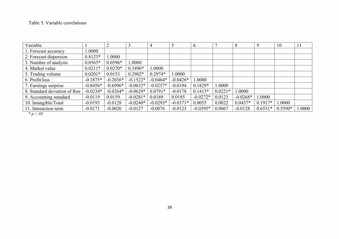
Table 5 provides the correlations of all variables. The two dependent variables, forecast

accuracy and forecast dispersion, are significantly correlated, indicating a relationship

whereby an increase in forecast accuracy correlates with a decrease in forecast dispersion.

Therefore, when analysts reach greater consensus, their EPS forecasts become more accurate.

None of these variables is significantly correlated with accounting standard followed or the

interaction term. Accounting standard followed and the interaction term correlate negatively

with forecast accuracy, which is counter to the hypothesized relationship, in which the

introduction of IFRS would increase forecast accuracy, particularly in firms with a higher

degree of intangible assets. The table also shows that all six control variables significantly

correlate with forecast accuracy. The signs indicate that the number of analysts, market value,

and trading volume are associated with increased forecast accuracy, whereas unprofitable

firms, earnings surprise and variation in profitability appear to worsen forecast accuracy.

These correlations all occur in the expected direction, as observed earlier in Table 1. The table

provides similar results for forecast dispersion, with the exception of trading volume, which is

not significant. There appear to be no problems with multicollinearity; the highest correlation

among the independent variables is 0.35 (for market value and number of analysts). However,

24 

 

as expected, a high positive correlation exists between accounting standard followed and the

interaction term. Nonetheless, all variance inflation factor (VIF) values are lower than 2; thus,

there is no reason to believe that this correlation is affecting the accuracy of the estimations.

------------------------------------------------------------

Insert Table 5 about here

-------------------------------------------------------------

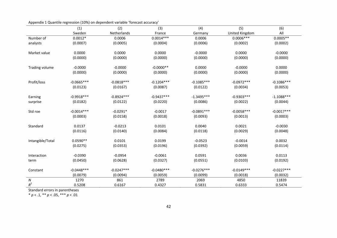
The complete results of the regressions are presented in appendices 1-6. The strongest

predictors of forecast accuracy and forecast dispersion are the control variables profit/loss and

earnings surprise, which have the expected signs in all cases except two (earnings surprise for

Sweden and the Netherlands, in appendix 6). Overall, the models have much higher

explanatory power when predicting the 10th percentile (Pseudo R2 from 0.43-0.63 for

estimations of equation 1 and 0.25-0.44 for estimations of equation 2) than when predicting

the 50th percentile (Pseudo R2 from 0.17-0.27 for equation 1 and 0.05-0.14 for equation 2) or

the 90th percentile (Pseudo R2 from 0.03-0.05 for equation 1 and 0.02-0.03 for equation 2).

This result indicates that smaller errors and dispersions are more random than systematic and,

therefore, should be little affected by a change in accounting standard.

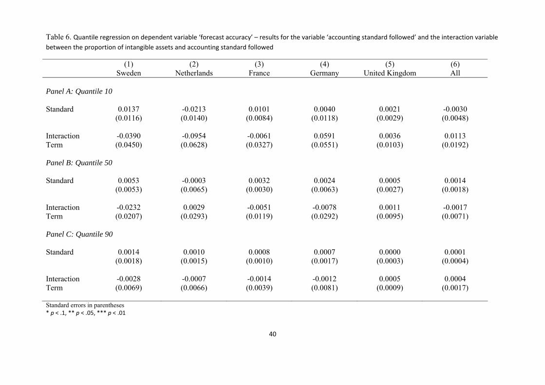
Table 6, which summarizes the results for the test variables from appendices 1-3, indicates

that IFRS have no measurable impact on forecast accuracy, either overall or for individual

countries, and that there are no measurable differences between firms with varying degrees of

intangible assets. None of the coefficients is significant and there is no consistency among the

signs of the coefficients. Therefore, in general, we fail to find evidence in support of H1 or

H5. Because we find no systematic difference between countries, the results support neither

25 

 

H3a nor H3b. IFRS appear to have no impact on forecast accuracy, regardless of prior GAAP-

difference or legal enforcement.

------------------------------------------------------------

Insert Table 6 about here

-------------------------------------------------------------

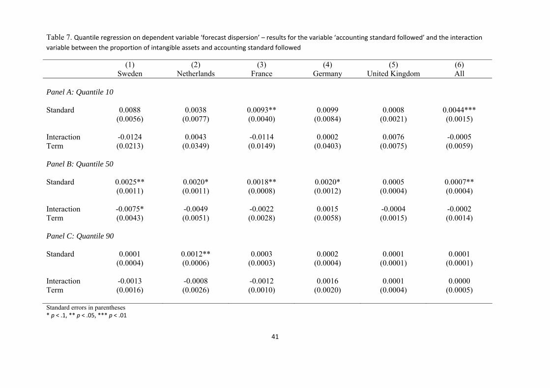
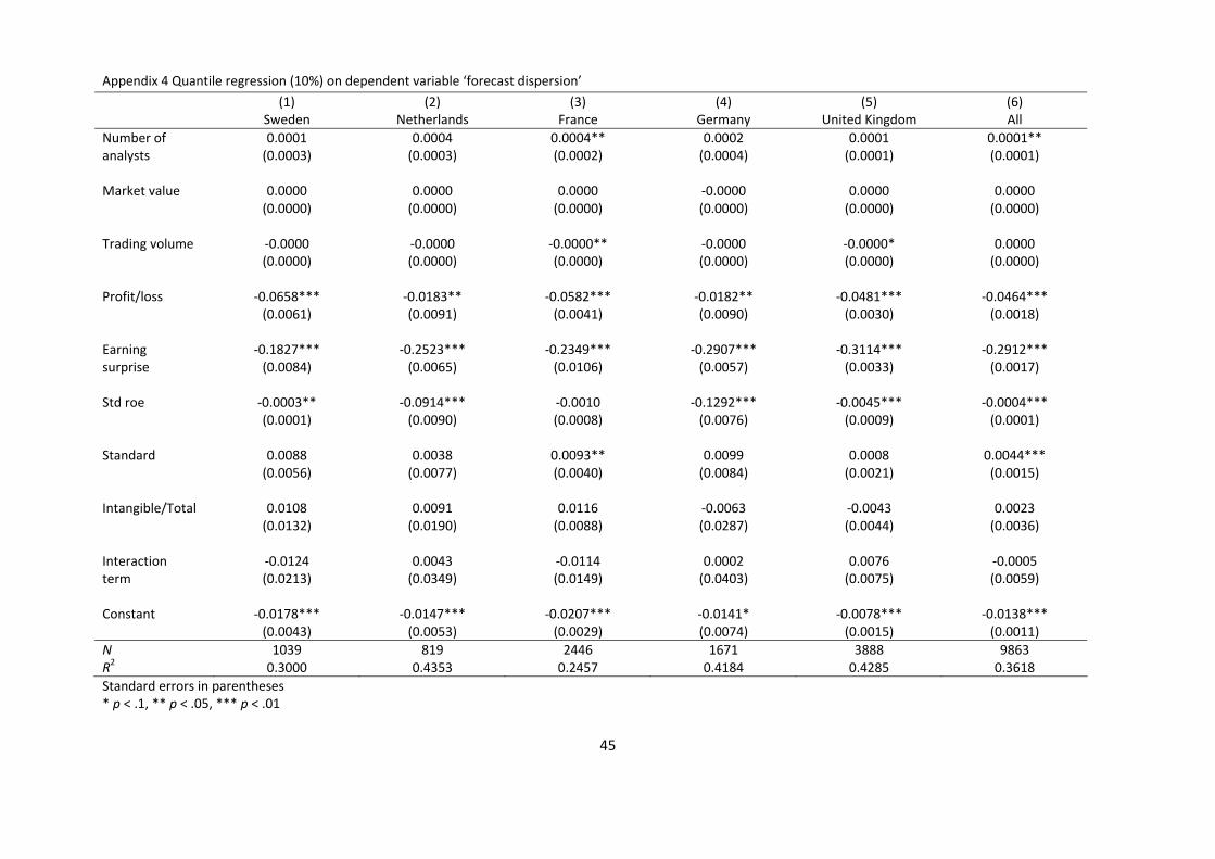
Table 7, which summarizes the results for the test variables from appendices 4-6, shows a

slightly more consistent pattern regarding forecast dispersion. All coefficients of the variable

accounting standard followed are positive and many are significant, indicating that IFRS

appears to result in diminished forecast dispersion. In particular, IFRS appears to have

affected forecast dispersion in the 50th percentile; the only exception is the UK, for which

there is a positive but insignificant coefficient. In the 10th percentile and the 90th percentile,

the effect is not equally consistent, but there is a significant positive effect in France and for

the full sample at the 10th percentile level and a significant positive effect in the Netherlands

at the 90th percentile level. However, the interaction term exhibits no consistent pattern. The

signs are mixed, and only one coefficient is significant, although it has a sign that is the

opposite of that expected.

------------------------------------------------------------

Insert Table 7 about here

-------------------------------------------------------------

These results provide some support for H2 but no support for H6. Although IFRS appear to

have a measurable impact on forecast dispersion, the degree of intangible asset appears not to

26 

 

affect this relationship. When examining cross-country differences, we note that in the UK,

forecast dispersion has not been affected by IFRS. The UK exhibits the smallest GAAP-

difference of all of the countries in the sample, which might explain why there is no effect on

forecast dispersion. At the same time, the UK has the strongest enforcement, which in theory,

should indicate a stronger effect. Another country with a low GAAP-difference is the

Netherlands, in which we detect an effect both in the 10th percentile and the 50th percentile,

which suggests that the impact of GAAP-difference is not so straightforward. The

Netherlands has the weakest enforcement in the sample but still displays positive significant

coefficients. The only other country that has two significant coefficients, in the 50th percentile

and in the 90th percentile, is France, which exhibits both a high GAAP-difference and strong

enforcement. That there is an effect in Sweden, a country with a large GAAP-difference but

weak enforcement, but not the UK, suggests that GAAP-difference is more important than

enforcement. Although the results for the Netherlands may appear to discredit this

interpretation, it is possible that GAAP-difference has a non-linear positive effect, suggesting

support for H4a. It is difficult to argue that enforcement has an effect based on our results,

indicating that H4b is likely false.

Broadly speaking, our results indicate that analysts have become more uniform in their

forecasts since the introduction of IFRS, suggesting that uncertainty among these

professionals has decreased. This decreased uncertainty appears not to be driven by IFRS

asset valuation methods’ better representation of firms’ underlying economic value because

the effect is not more pronounced in firms with higher degrees of intangible assets.

27 

 

5. Robustness analysis

As an alternative procedure, we have also estimated our equations using OLS regressions.

Because contrary to quantile regression, OLS is sensitive to skewness and outliers, the sample

was winsorized. A total of 2.5 percent of each tail was altered during this process, which

should resolve the outlier problem. The sample is still highly skewed, so the risk of biased

estimators remains and the result should be interpreted with caution. The estimated models

are provided in appendices 7-8.

The result for forecast accuracy differs slightly from that obtained using quantile regression.

There is a small but significant positive effect in Sweden and France, whereas there is a

significant and negative effect in the UK. We find no significant effect for the sample as a

whole. Obviously, these effects are not consistent and, because of the remaining skewness of

the sample, this result might be viewed as being uncertain. However, it is possible to argue

that this result suggests that IFRS have increased forecast accuracy in Sweden and France

while decreasing it in the UK. The interaction term is significant and positive for Germany

but not for any other country or overall. The result for forecast dispersion is practically the

same as that obtained using quantile regression. We record a positive effect of IFRS in all

countries except the UK. Three countries (Sweden, France and Germany) exhibit significant

interaction terms, but these point in different directions.

The OLS estimations thus do little to challenge the overall pattern identified in the data.

Although a few more coefficients become significant, there is no consistent pattern, which

causes us to suspect that they are spurious.

28 

 

6. Conclusions

In summary, our results demonstrate that IFRS have no impact on financial analysts’ forecast

accuracy but a more consistent impact on forecast dispersion, which has diminished in all

countries in the sample except the UK. These results appear not to be driven by the asset

valuation methods of IFRS, but the difference between IFRS and prior GAAP appears to have

an impact.

Prior research suggests that IAS/IFRS have a positive effect on analyst performance overall

(e.g., Ashbaugh and Pincus, 2001; Jiao et al., 2012) or at least if accounting standard

enforcement is strong (Byard et al., 2011; Horton et al., 2012; Preiato et al., 2010), prior

GAAP differ from IFRS (Beuselinck et al., 2010), or prior disclosure standards were of high

quality (Yang, 2010). Our study contributes to this literature because we combine a long time

period with a consistent estimation method that allows us to estimate the impact of IFRS on

both large and small errors without assuming the same impact for the entire distribution and

introduce a new proxy that allows us to determine whether it is the asset measurement

methods of IFRS that affect accounting quality. Our results differ slightly in that we find no

overall improvement in forecast accuracy regardless of prior GAAP-difference or

enforcement, whereas the impact of forecast dispersion is more broad and positive. The only

country in our sample that did not see a diminished forecast dispersion was the UK, a country

in which enforcement is strong and GAAP-difference is minimal. Because Sweden, a country

with weak enforcement of accounting standards but a significant GAAP-difference, displays

decreasing forecast dispersion, our results suggest, in line with Beuselinck et al. (2010), that

GAAP-difference is the crucial factor.

29 

 

Because forecast dispersion is a measure of information asymmetry (Krishnaswami and

Subramaniam, 1999), we claim that some aspect of information asymmetry has likely

decreased under IFRS although forecast accuracy has not increased. This effect is an

indication that analysts have a more even playing field, suggesting that some previously

private or withheld information is now available to more analysts, which would explain why

forecast dispersion has decreased. This explanation would imply that the qualitative increase

produced by IFRS may therefore be more connected to increasing information harmonization

and comparability than with making firms’ financial reports more accurately represent

underlying economic value. Standard setters argue that fair value accounting provides more

relevant information for predictions of firm performance (Hitz, 2007). If this is the case,

perhaps analysts processed accounting numbers acquired from historical cost accounting to

obtain estimates of fair value under their local GAAP. With IFRS, this processing is no longer

as necessary, as it is conducted by firms themselves. This method is likely to result in less

forecast dispersion because all analysts will have access to the same fair value accounting

numbers, although on average, these estimates may not be superior to the average estimates

processed under national GAAP. If this interpretation is correct, the implication is that IFRS

accounting methods create a more level playing field for accounting users but without

necessarily producing higher predictive value. Another more speculative implication is that

fair value accounting (which is more pronounced in IFRS than in previous GAAP) is

preferred over historical cost accounting by financial analysts.

Soderstrom and Sun (2007) argue that there is a direct link between accounting standard and

accounting quality. If this link exists, transitioning to an accounting standard of higher quality

should increase accounting quality. Our results imply that it is fruitful to distinguish between

how accounting quality affects users’ accuracy and how it affects users’ consistency.

30 

 

Although IFRS appears to affect consistency, we have little evidence to suggest that it affects

users’ accuracy. Therefore, IFRS can be viewed as a standard of higher quality than

previously used local accounting standards in Sweden, France, the Netherlands and Germany,

but only in the sense of consistency. This conclusion would appear to imply that there is a

need to develop additional measures of accounting quality that consider this distinction for

both practical and research applications because it is difficult to see how the standard

measures of accounting quality (earnings management, timely loss recognition and value

relevance) can capture this dimension.

A number of factors beyond the standards themselves could explain the limited effect of IFRS

on analyst performance. Our empirical design has limited power in isolating the effects of

IFRS from those of, for example, general macroeconomic changes or general developments in

financial markets. However, we do use control variables to mitigate those time periods in

which the job of prediction is especially troublesome. Another design limitation is the

assumption that financial analysts use financial reports as a primary source of information

when formulating predictions. Although this idea is supported by the literature (Block, 1999;

Roger and Grant, 1997) and our findings regarding forecast dispersion, more thorough

documentation is needed to demonstrate how analysts actually use financial reports for

developing forecasts and how different sources of information relate to one another. Such

documentation will aid us in gaining a better understanding of the effects of changing

accounting standards. A number of previous studies (Ball, 2006; Zeff, 2007) suggest that the

implementation of IFRS will not have a uniform impact in all countries and that

implementation will take time. Kvaal and Nobes (2012) find that national patterns still

prevail. Our design is likely better suited to distinguishing between immediate and uniform

effects.

31 

 

Despite these limitations, we conclude that when evaluated from a decision usefulness

perspective, IFRS has limited impact on accounting quality in the examined countries;

however, this impact is connected more to the presentation of more consistent pictures for

predictions of firm performance than to the presentation of more accurate pictures.

References

Ali, A. and Hwang, L. (2000) Country-Specific Factors Related to Financial Reporting and

the Value Relevance of Accounting Data, Journal of Accounting Research, 38(1), pp. 1-21

Armstrong, Christopher S., Barth, Mary E., Jagolinzer, Alan D. and Riedl, Edward J. (2010)

Market Reaction to the Adoption of IFRS in Europe, Accounting Review, 85(1), pp. 31-61

Ashbaugh, H. and Pincus, M. (2001) Domestic accounting standards, international accounting

standards, and the predictability of earnings, Journal of Accounting Research, 39(3), pp. 417-

434.

Bae, K., Tan, H. and Welker, M. (2008) International GAAP differences: the impact on

foreign analysts, The Accounting Review, 83, pp. 593-628.

Ball, R., Kothari, S., and Robin, A. (2000) The effect of international institutional factors on

properties of accounting earnings, Journal of Accounting and Economics, 29, pp. 1-51.

Ball, R. (2006) International Financial Reporting Standards (IFRS): pros and cons for

investors, Accounting & Business Research, 36, pp. 5-27.

Barry, C. and Brown, S. (1985) Differential Information and Security Market Equilibrium,

Journal of Financial and Quantitative Analysis , 20, pp. 407–422.

Barth, M.E., Landsman, W.R. and Lang, M.H. (2008) International accounting standards and

accounting quality, Journal of Accounting Research 46(3), pp. 467-498.

Bartov, E., Goldberg, S.R. and Myungsun, K. (2005) Comparative Value Relevance Among

German, U.S., and International Accounting Standards: A German Stock Market Perspective,

Journal of Accounting, Auditing and Finance, 20(2), pp. 95-120.

32 

 

Bradshaw, M. T. (2004) How Do Analysts Use Their Earnings Forecasts in Generating Stock

Recommendations, Accounting Review , 79(1), pp. 25-50.

Brennan, M. and Hughes, P. (1991) Stock Prices and the Supply of Information, Journal of

Finance, 46(5), pp. 1665-1691.

Block, S. (1999) A study of financial analysts: practice and theory, Financial Analysts

Journal, 55(4), pp. 86-95.

Byard, D., Li, Y. and Yu, Y. (2011) The Effect of Mandatory IFRS Adoption on Financial

Analysts’ Information Environment, Journal of Accounting Research, 49(1), pp. 69-96.

Dao, T. (2005) Monitoring Compliance with IFRS: Some Insights from the French

Regulatory System, Accounting in Europe, 2, pp. 107-135.

Daske, H. and Gebhardt, G. (2006) International Financial Reporting Standards and Experts

Perceptions of Disclosure Quality, Abacus, 42, pp. 461-498.

Daske, H., Hail, L., Leuz, C. and Verdi, R. (2008) Mandatory IFRS Reporting around the

World: Early Evidence on the Economic Consequences, Journal of Accounting Research,

46(5), pp. 1085-1142.

Ding, Y., Hope, O.-K., Jeanjean, T. and Stolowy, H. (2007) Differences between domestic

accounting standards and IAS: Measurement, determinants and implications, Journal of

Accounting and Public Policy , 26(1), pp. 1-38.

EU (2002) European Union, EC regulation No 1606/2002. Available at: http://eur-

lex.europa.eu/

Francis, J., Khurana, I. and Pereira, R. (2003) The role of accounting and auditing in

corporate governance and the development of financial markets around the world, Asia-

Pacific Journal of Accounting and Economics , 10, pp. 1-30.

Glaum, M., Baetge, J., Grothe, A. and Oberdorster, T. (forthcoming) Introduction of

International Accounting Standards, disclosure quality and accuracy of analysts’ earnings

forecasts, forthcoming in European Accounting Review.

33 

 

Glosten, L. and Milgrom, P. (1985) Bid, Ask, and Transaction Prices in a Specialist Market

with Heterogeneously Informed Traders, Journal of Financial Economics, 26, pp. 71–100.

Heflin, F., Subramanyam K. and Zhang, Y. (2003) Regulation FD and the financial

information environment: Early evidence, The Accounting Review, 78(1), pp. 1-37.

Hitz, J-M. (2007) The decision usefulness of fair value accounting – a theoretical perspective,

European Accounting Review, 16(2), pp. 323-362.

Hope, O. (2003) Disclosure practices, enforcement of accounting standards, and analysts’

forecast accuracy: An international study, Journal of Accounting Research, 41(2), pp. 235-

272.

Hung, M. and Subramanyam, K.R. (2007) Financial statement effects of adopting

international accounting standards: the case of Germany, Review of Accounting Studies, 12,

pp. 623-657.

IASB (2010). International Accounting Standards Board, Conceptual Framework. Available

at: http://www.ifrs.org

Irani, A. and Karamanou, I. (2003) Regulation Fair Disclosure, analyst following, and analyst

forecast dispersion, Accounting Horizons,17(1), pp. 15-29.

Jeanjean, T. and Stolowy, H. (2008) Do accounting standards matter? An exploratory

analysis of earnings management before and after IFRS adoption, Journal of Accounting and

Public Policy, 27, pp. 480-494.

Jiao, T., Koning, M., Mertens, G. and Roosenboom, P. (2012) Mandatory IFRS adoption and

its impact on analysts’ forecasts, International Review of Financial Analysis, 21, pp. 56-63.

King, R., Pownall, G. and Waymire, B. (1990) Expectations adjustments via timely

management forecasts: Review, synthesis, and suggestions for future research, Journal of

Accounting Literature, 31(2), pp. 113-144.

Koenker, R. and Basset, G. (1978) Regression quantiles, Econometrica, 46, pp. 33-50.

Krishnaswami, S. and Subramaniam, V. (1999) Information Asymmetry, Valuation, and the

Corporate Spin-off Decision, Journal of Financial Economics, 53, pp. 73–112.

34 

 

Kvaal, E. and Nobes, C. (2012) IFRS policy changes and the continuation of national patterns

of IFRS practice, European Accounting Review, 21, pp. 343-371.

La Porta, R., Lopez-de-Silanes, F., Shleifer, A. and Vishny, R. (1998) Law and finance,

Journal of Political Economy, 106( 6), pp. 1113-1155.

Lang, M. and Lundholm, R. (1993) Cross-Sectional Determinants of Analyst Ratings of

Corporate Disclosures, Journal of Accounting Research, 31(2), pp. 246-271.

Lang, M. H. and Lundholm, R. J. (1996) Corporate Disclosure Policy and Analyst Behavior,

The Accounting Review , 71(4), pp. 467–492.

Leuz, C., Nanda, D. and Wysocki, P. (2003) Investor protection and earnings management: an

international comparison, Journal of Financial Economics , 69, pp. 505–527.

Merton, R. (1987) Presidential Address: A simple model of capital market equilibrium with

incomplete information, Journal of Finance , 42, pp. 483–510.

Ormrod, P. and Taylor, P. (2004) The impact of the change to International Accounting

Standards on debt covenants: a UK perspective, Accounting in Europe, 1, pp. 71-94.

Ramnath, S., Rock, S. and Shane, P. (2008) The financial analyst forecasting literature: A

taxonomy with suggestions for further research, International Journal of Forecasting, 24(1),

pp. 34-75.

Revsine, L., Collins, D. W. and Johnson, W. B. (2004) Financial Reporting and Analysis, 2nd

edn (Prentice Hall, Upper Saddle River, NJ).

Rogers, R. and Grant, J. (1997) Content analysis of information cited in reports of sell-side

financial analysts, Journal of Financial Statement Analysis, 3(1), pp. 17-30.

Schipper, K. (1991) Analysts’ Forecasts, Accounting Horizons, 4, pp. 105–121.

Soderstrom, N. and Sun, K. (2007) IFRS Adoption and Accounting Quality: A Review,

European Accounting Review, 16(4), pp. 675-702.

Zeff, S. (2007) Some obstacles to global financial reporting comparability and convergence at

a high level of quality, British Accounting Review, 39(4), pp. 290-302.

35 

 

Table 1. GAAP difference and enforcement

   GAAP‐difference Bae et al. 2008 

Enforcement Preiato et al. 2010 

Sweden  10  14Netherlands  4  12

France  12  21Germany  11  18

United Kingdom  1  24

36 

 

Table 2. Independent variables Variable Explanation Predicted sign of the

dependent variables Number of analysts The number of analysts following a company. + Market value Market value is measured as the company’s

market value at the beginning of the fiscal year. +

Trading volume Trading volume refers to the company’s absolute daily trading volume during the first month of the fiscal year.

+

Profit/Loss Loss, a dummy variable that takes the value of 1 if the company reported a loss and 0 otherwise.

-

Earnings surprise The absolute value of the year’s earnings per share, minus the previous year’s earnings per share, scaled by the share price at the beginning of the fiscal year. EPSt is the earnings per share during period t (of a given year), and EPSt-1 is the earnings per share in period t-1 (the previous year).

-

Std ROE The company’s standard deviation return on equity over the previous three years.

-

Accounting standard followed

A dummy variable that takes the value of 1 if the company used IFRS for preparing last years’ financial reports and 0 otherwise.

+

Proportion of intangible assets

Reported value of intangible assets divided by reported total assets.

?

Interaction term Accounting standard followed multiplied by proportion of intangible assets.

+

37 

 

Table 3. Sample statistics

Number of observations Mean Std Dev

Country Number

of firms Total

sample

Valid

Forecast

accuracy

Valid

Forecast

dispersion

Forecast

accuracy

Forecast

dispersion

Forecast

accuracy

Forecast

dispersion

Sweden 259 1829 1829 1460 -0.0633 -0.0201 0.1748 0.0424

Netherlands 93 1064 1064 1043 -0.0562 -0.0170 0.3111 0.0622

France 635 3836 3836 3404 -0.0613 -0.0182 0.2298 0.0615

Germany 647 3797 3797 3186 -0.1139 -0.0390 0.5477 0.2323

UK 813 6923 6923 5910 -0.0380 -0.0125 0.1718 0.0568

All 2447 17449 17449 15003 -0.0634 -0.0205 0.3138 0.1189

38 

 

Table 4. Medians and percentiles  

Significant difference comparing medians pre and post IFRS * p < .05 

25th percentile Median 75th percentile Median

Forecast accuracy

Median

Forecast dispersion Country

Forecast

accuracy

Forecast

dispersion

Forecast

accuracy

Forecast

dispersion

Forecast

accuracy

Forecast

dispersion

Pre IFRS Post IFRS Pre IFRS Post IFRS

Sweden -0.0627 -0.0178 -0.0245 -0.0088 -0.0091 -0.0044 -0.0260* -0.0190* -0.0094* -0.0076*

Netherlands -0.0414 -0.0127 -0.0172 -0.0056 -0.0070 -0.0024 -0.0164 -0.0190 -0.0057 -0.0054

France -0.0462 -0.0152 -0.0177 -0.0068 -0.0066 -0.0033 -0.0179 -0.0174 -0.0074* -0.0061*

Germany -0.0724 -0.0190 -0.0257 -0.0074 -0.0088 -0.0034 -0.0234* -0.0282* -0.0076 -0.0072

UK -0.0263 -0.0082 -0.0101 -0.0036 -0.0032 -0.0015 -0.0105* -0.0093* -0.0036 -0.0033

All -0.0439 -0.0129 -0.0157 -0.0056 -0.0053 -0.0024 -0.0152* -0.0163* -0.0056 -0.0055

39 

 

Table 5. Variable correlations

Variable 1 2 3 4 5 6 7 8 9 10 11 1. Forecast accuracy 1.0000 2. Forecast dispersion 0.8123* 1.0000 3. Number of analysts 0.0565* 0.0596* 1.0000 4. Market value 0.0211* 0.0270* 0.3496* 1.0000 5. Trading volume 0.0201* 0.0153 0.2902* 0.2974* 1.0000 6. Profit/loss -0.1875* -0.2036* -0.1522* -0.0464* -0.0426* 1.0000 7. Earnings surprise -0.8456* -0.6996* -0.0632* -0.0257* -0.0194 0.1829* 1.0000 8. Standard deviation of Roe -0.0234* -0.0264* -0.0629* 0.0791* -0.0178 0.1415* 0.0221* 1.0000 9. Accounting standard -0.0119 0.0159 -0.0281* 0.0189 0.0185 -0.0272* 0.0123 -0.0268* 1.0000 10. Intangible/Total -0.0193 -0.0128 -0.0240* -0.0293* -0.0371* 0.0055 0.0022 0.0437* 0.1917* 1.0000 11. Interaction term -0.0171 -0.0026 -0.0127 -0.0076 -0.0123 -0.0395* 0.0067 -0.0128 0.6531* 0.5590* 1.0000

* p < .05 

40 

 

Table 6. Quantile regression on dependent variable ‘forecast accuracy’ – results for the variable ‘accounting standard followed’ and the interaction variable between the proportion of intangible assets and accounting standard followed 

(1) (2) (3) (4) (5) (6) Sweden Netherlands France Germany United Kingdom All Panel A: Quantile 10 Standard 0.0137 -0.0213 0.0101 0.0040 0.0021 -0.0030 (0.0116) (0.0140) (0.0084) (0.0118) (0.0029) (0.0048) Interaction -0.0390 -0.0954 -0.0061 0.0591 0.0036 0.0113 Term (0.0450) (0.0628) (0.0327) (0.0551) (0.0103) (0.0192) Panel B: Quantile 50 Standard 0.0053 -0.0003 0.0032 0.0024 0.0005 0.0014 (0.0053) (0.0065) (0.0030) (0.0063) (0.0027) (0.0018) Interaction -0.0232 0.0029 -0.0051 -0.0078 0.0011 -0.0017 Term (0.0207) (0.0293) (0.0119) (0.0292) (0.0095) (0.0071) Panel C: Quantile 90 Standard 0.0014 0.0010 0.0008 0.0007 0.0000 0.0001 (0.0018) (0.0015) (0.0010) (0.0017) (0.0003) (0.0004) Interaction -0.0028 -0.0007 -0.0014 -0.0012 0.0005 0.0004 Term (0.0069) (0.0066) (0.0039) (0.0081) (0.0009) (0.0017) Standard errors in parentheses * p < .1, ** p < .05, *** p < .01

41 

 

Table 7. Quantile regression on dependent variable ‘forecast dispersion’ – results for the variable ‘accounting standard followed’ and the interaction variable between the proportion of intangible assets and accounting standard followed 

(1) (2) (3) (4) (5) (6) Sweden Netherlands France Germany United Kingdom All Panel A: Quantile 10 Standard 0.0088 0.0038 0.0093** 0.0099 0.0008 0.0044*** (0.0056) (0.0077) (0.0040) (0.0084) (0.0021) (0.0015) Interaction -0.0124 0.0043 -0.0114 0.0002 0.0076 -0.0005 Term (0.0213) (0.0349) (0.0149) (0.0403) (0.0075) (0.0059) Panel B: Quantile 50 Standard 0.0025** 0.0020* 0.0018** 0.0020* 0.0005 0.0007** (0.0011) (0.0011) (0.0008) (0.0012) (0.0004) (0.0004) Interaction -0.0075* -0.0049 -0.0022 0.0015 -0.0004 -0.0002 Term (0.0043) (0.0051) (0.0028) (0.0058) (0.0015) (0.0014) Panel C: Quantile 90 Standard 0.0001 0.0012** 0.0003 0.0002 0.0001 0.0001 (0.0004) (0.0006) (0.0003) (0.0004) (0.0001) (0.0001) Interaction -0.0013 -0.0008 -0.0012 0.0016 0.0001 0.0000 Term (0.0016) (0.0026) (0.0010) (0.0020) (0.0004) (0.0005) Standard errors in parentheses * p < .1, ** p < .05, *** p < .01

42 

 

Appendix 1 Quantile regression (10%) on dependent variable ‘forecast accuracy’ 

  (1)  (2)  (3)  (4)  (5)  (6)   Sweden  Netherlands  France  Germany  United Kingdom  All Number of   0.0012*  0.0006  0.0014***  0.0006  0.0006***  0.0005** analysts  (0.0007)  (0.0005)  (0.0004)  (0.0006)  (0.0002)  (0.0002)              Market value  0.0000  0.0000  0.0000  ‐0.0000  0.0000  ‐0.0000   (0.0000)  (0.0000)  (0.0000)  (0.0000)  (0.0000)  (0.0000)              Trading volume  ‐0.0000  ‐0.0000  ‐0.0000**  0.0000  ‐0.0000  0.0000   (0.0000)  (0.0000)  (0.0000)  (0.0000)  (0.0000)  (0.0000)              Profit/loss  ‐0.0665***  ‐0.0818***  ‐0.1204***  ‐0.1085***  ‐0.0972***  ‐0.1086***   (0.0123)  (0.0167)  (0.0087)  (0.0122)  (0.0034)  (0.0053)              Earning   ‐0.9918***  ‐0.8924***  ‐0.9437***  ‐1.3495***  ‐0.9303***  ‐1.1088*** surprise  (0.0182)  (0.0122)  (0.0220)  (0.0086)  (0.0022)  (0.0044)              Std roe  ‐0.0014***  ‐0.0291*  ‐0.0017  ‐0.0891***  ‐0.0058***  ‐0.0017***   (0.0003)  (0.0158)  (0.0018)  (0.0093)  (0.0013)  (0.0003)              Standard  0.0137  ‐0.0213  0.0101  0.0040  0.0021  ‐0.0030   (0.0116)  (0.0140)  (0.0084)  (0.0118)  (0.0029)  (0.0048)              Intangible/Total  0.0590**  0.0101  0.0199  ‐0.0523  ‐0.0014  0.0032   (0.0275)  (0.0353)  (0.0196)  (0.0392)  (0.0059)  (0.0114)              Interaction  ‐0.0390  ‐0.0954  ‐0.0061  0.0591  0.0036  0.0113 term  (0.0450)  (0.0628)  (0.0327)  (0.0551)  (0.0103)  (0.0192)              Constant  ‐0.0448***  ‐0.0247***  ‐0.0480***  ‐0.0276***  ‐0.0149***  ‐0.0227***   (0.0079)  (0.0094)  (0.0059)  (0.0099)  (0.0018)  (0.0032) N  1270  861  2789  2069  4850  11839 R2  0.5208  0.6167  0.4327  0.5831  0.6333  0.5474 Standard errors in parentheses * p < .1, ** p < .05, *** p < .01  

43 

 

Appendix 2 Quantile regression (50%) on dependent variable ‘forecast accuracy’ 

  (1)  (2)  (3)  (4)  (5)  (6)   Sweden  Netherlands  France  Germany  United Kingdom  All Number of   0.0000  0.0001  0.0002  0.0002  0.0003*  0.0001 analysts  (0.0003)  (0.0002)  (0.0001)  (0.0003)  (0.0002)  (0.0001)              Market value  0.0000  0.0000  0.0000  ‐0.0000  0.0000  0.0000   (0.0000)  (0.0000)  (0.0000)  (0.0000)  (0.0000)  (0.0000)              Trading volume  0.0000  ‐0.0000  ‐0.0000  0.0000  ‐0.0000  0.0000   (0.0000)  (0.0000)  (0.0000)  (0.0000)  (0.0000)  (0.0000)              Profit/loss  ‐0.0466***  ‐0.0707***  ‐0.0607***  ‐0.0570***  ‐0.0325***  ‐0.0486***   (0.0056)  (0.0078)  (0.0032)  (0.0064)  (0.0031)  (0.0020)              Earning   ‐0.3075***  ‐0.5297***  ‐0.3092***  ‐0.5584***  ‐0.3739***  ‐0.4424*** surprise  (0.0084)  (0.0057)  (0.0080)  (0.0046)  (0.0021)  (0.0016)              Std roe  ‐0.0005***  0.0020  ‐0.0008  0.0021  ‐0.0009  ‐0.0003***   (0.0001)  (0.0073)  (0.0006)  (0.0049)  (0.0012)  (0.0001)              Standard  0.0053  ‐0.0003  0.0032  0.0024  0.0005  0.0014   (0.0053)  (0.0065)  (0.0030)  (0.0063)  (0.0027)  (0.0018)              Intangible/Total  0.0234*  0.0058  0.0069  0.0004  ‐0.0029  ‐0.0002   (0.0126)  (0.0165)  (0.0072)  (0.0208)  (0.0054)  (0.0042)              Interaction  ‐0.0232  0.0029  ‐0.0051  ‐0.0078  0.0011  ‐0.0017 term  (0.0207)  (0.0293)  (0.0119)  (0.0292)  (0.0095)  (0.0071)              Constant  ‐0.0100***  ‐0.0093**  ‐0.0115***  ‐0.0064  ‐0.0057***  ‐0.0056***   (0.0036)  (0.0044)  (0.0022)  (0.0052)  (0.0017)  (0.0012) N  1270  861  2789  2069  4850  11839 R2  0.1834  0.2693  0.1684  0.2419  0.1878  0.2021 Standard errors in parentheses * p < .1, ** p < .05, *** p < .01  

44 

 

Appendix 3 Quantile regression (90%) on dependent variable ‘forecast accuracy’ 

  (1)  (2)  (3)  (4)  (5)  (6)   Sweden  Netherlands  France  Germany  United Kingdom  All Number of   0.0000  ‐0.0000  0.0000  0.0001  0.0000***  0.0000 analysts  (0.0001)  (0.0001)  (0.0000)  (0.0001)  (0.0000)  (0.0000)              Market value  0.0000  0.0000  ‐0.0000  ‐0.0000  0.0000  0.0000   (0.0000)  (0.0000)  (0.0000)  (0.0000)  (0.0000)  (0.0000)              Trading volume  ‐0.0000  ‐0.0000  0.0000  0.0000  ‐0.0000  0.0000   (0.0000)  (0.0000)  (0.0000)  (0.0000)  (0.0000)  (0.0000)              Profit/loss  ‐0.0208***  ‐0.0195***  ‐0.0155***  ‐0.0206***  ‐0.0024***  ‐0.0094***   (0.0019)  (0.0018)  (0.0011)  (0.0018)  (0.0003)  (0.0005)              Earning   ‐0.0086***  ‐0.0413***  ‐0.0474***  ‐0.0682***  ‐0.0224***  ‐0.0318*** surprise  (0.0028)  (0.0013)  (0.0026)  (0.0013)  (0.0002)  (0.0004)              Std roe  ‐0.0000  ‐0.0024  ‐0.0001  ‐0.0011  ‐0.0002  ‐0.0001***   (0.0000)  (0.0017)  (0.0002)  (0.0014)  (0.0001)  (0.0000)              Standard  0.0014  0.0010  0.0008  0.0007  0.0000  0.0001   (0.0018)  (0.0015)  (0.0010)  (0.0017)  (0.0003)  (0.0004)              Intangible/Total  0.0048  ‐0.0014  ‐0.0002  0.0008  ‐0.0003  ‐0.0003   (0.0042)  (0.0037)  (0.0024)  (0.0058)  (0.0005)  (0.0010)              Interaction  ‐0.0028  ‐0.0007  ‐0.0014  ‐0.0012  0.0005  0.0004 term  (0.0069)  (0.0066)  (0.0039)  (0.0081)  (0.0009)  (0.0017)              Constant  ‐0.0039***  ‐0.0015  ‐0.0018**  ‐0.0020  ‐0.0010***  ‐0.0013***   (0.0012)  (0.0010)  (0.0007)  (0.0015)  (0.0002)  (0.0003) N  1270  861  2789  2069  4850  11839 R2  0.0275  0.0471  0.0343  0.0453  0.0281  0.0266 Standard errors in parentheses * p < .1, ** p < .05, *** p < .01  

45 

 

Appendix 4 Quantile regression (10%) on dependent variable ‘forecast dispersion’ 

  (1)  (2)  (3)  (4)  (5)  (6)   Sweden  Netherlands  France  Germany  United Kingdom  All Number of   0.0001  0.0004  0.0004**  0.0002  0.0001  0.0001** analysts  (0.0003)  (0.0003)  (0.0002)  (0.0004)  (0.0001)  (0.0001)              Market value  0.0000  0.0000  0.0000  ‐0.0000  0.0000  0.0000   (0.0000)  (0.0000)  (0.0000)  (0.0000)  (0.0000)  (0.0000)              Trading volume  ‐0.0000  ‐0.0000  ‐0.0000**  ‐0.0000  ‐0.0000*  0.0000   (0.0000)  (0.0000)  (0.0000)  (0.0000)  (0.0000)  (0.0000)              Profit/loss  ‐0.0658***  ‐0.0183**  ‐0.0582***  ‐0.0182**  ‐0.0481***  ‐0.0464***   (0.0061)  (0.0091)  (0.0041)  (0.0090)  (0.0030)  (0.0018)              Earning   ‐0.1827***  ‐0.2523***  ‐0.2349***  ‐0.2907***  ‐0.3114***  ‐0.2912*** surprise  (0.0084)  (0.0065)  (0.0106)  (0.0057)  (0.0033)  (0.0017)              Std roe  ‐0.0003**  ‐0.0914***  ‐0.0010  ‐0.1292***  ‐0.0045***  ‐0.0004***   (0.0001)  (0.0090)  (0.0008)  (0.0076)  (0.0009)  (0.0001)              Standard  0.0088  0.0038  0.0093**  0.0099  0.0008  0.0044***   (0.0056)  (0.0077)  (0.0040)  (0.0084)  (0.0021)  (0.0015)              Intangible/Total  0.0108  0.0091  0.0116  ‐0.0063  ‐0.0043  0.0023   (0.0132)  (0.0190)  (0.0088)  (0.0287)  (0.0044)  (0.0036)              Interaction  ‐0.0124  0.0043  ‐0.0114  0.0002  0.0076  ‐0.0005 term  (0.0213)  (0.0349)  (0.0149)  (0.0403)  (0.0075)  (0.0059)              Constant  ‐0.0178***  ‐0.0147***  ‐0.0207***  ‐0.0141*  ‐0.0078***  ‐0.0138***   (0.0043)  (0.0053)  (0.0029)  (0.0074)  (0.0015)  (0.0011) N  1039  819  2446  1671  3888  9863 R2  0.3000  0.4353  0.2457  0.4184  0.4285  0.3618 Standard errors in parentheses * p < .1, ** p < .05, *** p < .01  

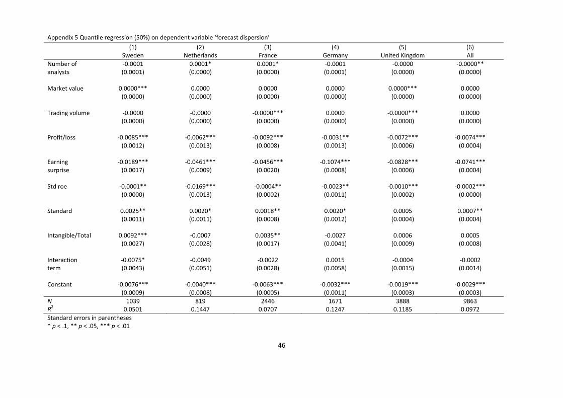
46 

 

Appendix 5 Quantile regression (50%) on dependent variable ‘forecast dispersion’ 

  (1)  (2)  (3)  (4)  (5)  (6)   Sweden  Netherlands  France  Germany  United Kingdom  All Number of   ‐0.0001  0.0001*  0.0001*  ‐0.0001  ‐0.0000  ‐0.0000** analysts  (0.0001)  (0.0000)  (0.0000)  (0.0001)  (0.0000)  (0.0000)              Market value  0.0000***  0.0000  0.0000  0.0000  0.0000***  0.0000   (0.0000)  (0.0000)  (0.0000)  (0.0000)  (0.0000)  (0.0000)              Trading volume  ‐0.0000  ‐0.0000  ‐0.0000***  0.0000  ‐0.0000***  0.0000   (0.0000)  (0.0000)  (0.0000)  (0.0000)  (0.0000)  (0.0000)              Profit/loss  ‐0.0085***  ‐0.0062***  ‐0.0092***  ‐0.0031**  ‐0.0072***  ‐0.0074***   (0.0012)  (0.0013)  (0.0008)  (0.0013)  (0.0006)  (0.0004)              Earning   ‐0.0189***  ‐0.0461***  ‐0.0456***  ‐0.1074***  ‐0.0828***  ‐0.0741*** surprise  (0.0017)  (0.0009)  (0.0020)  (0.0008)  (0.0006)  (0.0004)              Std roe  ‐0.0001**  ‐0.0169***  ‐0.0004**  ‐0.0023**  ‐0.0010***  ‐0.0002***   (0.0000)  (0.0013)  (0.0002)  (0.0011)  (0.0002)  (0.0000)              Standard  0.0025**  0.0020*  0.0018**  0.0020*  0.0005  0.0007**   (0.0011)  (0.0011)  (0.0008)  (0.0012)  (0.0004)  (0.0004)              Intangible/Total  0.0092***  ‐0.0007  0.0035**  ‐0.0027  0.0006  0.0005   (0.0027)  (0.0028)  (0.0017)  (0.0041)  (0.0009)  (0.0008)              Interaction  ‐0.0075*  ‐0.0049  ‐0.0022  0.0015  ‐0.0004  ‐0.0002 term  (0.0043)  (0.0051)  (0.0028)  (0.0058)  (0.0015)  (0.0014)              Constant  ‐0.0076***  ‐0.0040***  ‐0.0063***  ‐0.0032***  ‐0.0019***  ‐0.0029***   (0.0009)  (0.0008)  (0.0005)  (0.0011)  (0.0003)  (0.0003) N  1039  819  2446  1671  3888  9863 R2  0.0501  0.1447  0.0707  0.1247  0.1185  0.0972 Standard errors in parentheses * p < .1, ** p < .05, *** p < .01  

47 

 

Appendix 6 Quantile regression (90%) on dependent variable ‘forecast dispersion’ 

  (1)  (2)  (3)  (4)  (5)  (6)   Sweden  Netherlands  France  Germany  United Kingdom  All Number of   ‐0.0002***  0.0000  ‐0.0000**  ‐0.0001***  ‐0.0000***  ‐0.0000*** analysts  (0.0000)  (0.0000)  (0.0000)  (0.0000)  (0.0000)  (0.0000)              Market value  0.0000***  0.0000*  0.0000***  0.0000  0.0000***  0.0000   (0.0000)  (0.0000)  (0.0000)  (0.0000)  (0.0000)  (0.0000)              Trading volume  ‐0.0000  ‐0.0000***  ‐0.0000  0.0000  ‐0.0000***  0.0000***   (0.0000)  (0.0000)  (0.0000)  (0.0000)  (0.0000)  (0.0000)              Profit/loss  ‐0.0017***  ‐0.0019***  ‐0.0018***  ‐0.0010**  ‐0.0005***  ‐0.0013***   (0.0005)  (0.0007)  (0.0003)  (0.0004)  (0.0001)  (0.0001)              Earning   0.0000  0.0009*  ‐0.0065***  ‐0.0126***  ‐0.0088***  ‐0.0087*** surprise  (0.0006)  (0.0005)  (0.0007)  (0.0003)  (0.0002)  (0.0001)              Std roe  0.0000  ‐0.0030***  ‐0.0001*  ‐0.0001  0.0001**  ‐0.0000***   (0.0000)  (0.0007)  (0.0001)  (0.0004)  (0.0000)  (0.0000)              Standard  0.0001  0.0012**  0.0003  0.0002  0.0001  0.0001   (0.0004)  (0.0006)  (0.0003)  (0.0004)  (0.0001)  (0.0001)              Intangible/Total  0.0027***  0.0002  0.0012*  ‐0.0007  ‐0.0000  0.0001   (0.0010)  (0.0014)  (0.0006)  (0.0014)  (0.0002)  (0.0003)              Interaction  ‐0.0013  ‐0.0008  ‐0.0012  0.0016  0.0001  0.0000 term  (0.0016)  (0.0026)  (0.0010)  (0.0020)  (0.0004)  (0.0005)              Constant  ‐0.0017***  ‐0.0012***  ‐0.0016***  ‐0.0008**  ‐0.0004***  ‐0.0006***   (0.0003)  (0.0004)  (0.0002)  (0.0004)  (0.0001)  (0.0001) N  1039  819  2446  1671  3888  9863 R2  0.0305  0.0212  0.0160  0.0266  0.0234  0.0158 Standard errors in parentheses * p < .1, ** p < .05, *** p < .01  

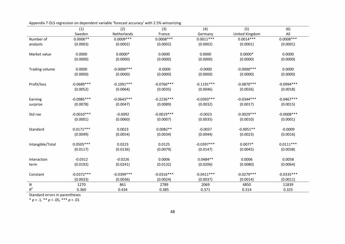
48 

 

Appendix 7 OLS regression on dependent variable ‘forecast accuracy’ with 2.5% winsorizing 

  (1)  (2)  (3)  (4)  (5)  (6)   Sweden  Netherlands  France  Germany  United Kingdom  All Number of   0.0006**  0.0009***  0.0008***  0.0011***  0.0014***  0.0008*** analysts  (0.0003)  (0.0002)  (0.0002)  (0.0002)  (0.0001)  (0.0001)              Market value  0.0000  0.0000*  0.0000  0.0000  0.0000*  0.0000   (0.0000)  (0.0000)  (0.0000)  (0.0000)  (0.0000)  (0.0000)              Trading volume  0.0000  ‐0.0000***  ‐0.0000  ‐0.0000  ‐0.0000***  0.0000   (0.0000)  (0.0000)  (0.0000)  (0.0000)  (0.0000)  (0.0000)              Profit/loss  ‐0.0689***  ‐0.1091***  ‐0.0760***  ‐0.1191***  ‐0.0870***  ‐0.0994***   (0.0052)  (0.0064)  (0.0035)  (0.0046)  (0.0026)  (0.0018)              Earning   ‐0.0985***  ‐0.0643***  ‐0.2236***  ‐0.0393***  ‐0.0344***  ‐0.0467*** surprise  (0.0078)  (0.0047)  (0.0089)  (0.0032)  (0.0017)  (0.0015)              Std roe  ‐0.0010***  ‐0.0092  ‐0.0019***  ‐0.0023  ‐0.0029***  ‐0.0008***   (0.0001)  (0.0060)  (0.0007)  (0.0035)  (0.0010)  (0.0001)              Standard  0.0171***  0.0023  0.0082**  ‐0.0037  ‐0.0051**  ‐0.0009   (0.0049)  (0.0054)  (0.0034)  (0.0044)  (0.0023)  (0.0016)              Intangible/Total  0.0505***  0.0223  0.0125  ‐0.0397***  0.0077*  0.0111***   (0.0117)  (0.0136)  (0.0079)  (0.0147)  (0.0045)  (0.0038)              Interaction  ‐0.0312  ‐0.0226  0.0006  0.0484**  0.0006  0.0058 term  (0.0192)  (0.0241)  (0.0132)  (0.0206)  (0.0080)  (0.0064)              Constant  ‐0.0372***  ‐0.0399***  ‐0.0316***  ‐0.0411***  ‐0.0279***  ‐0.0335***   (0.0033)  (0.0036)  (0.0024)  (0.0037)  (0.0014)  (0.0011) N  1270  861  2789  2069  4850  11839 R2  0.360  0.434  0.385  0.371  0.314  0.325 Standard errors in parentheses * p < .1, ** p < .05, *** p < .01  

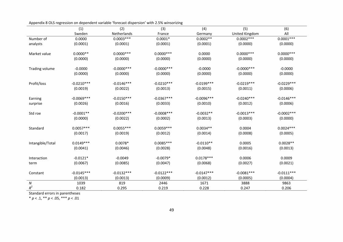
49 

 

Appendix 8 OLS regression on dependent variable ‘forecast dispersion’ with 2.5% winsorizing 

  (1)  (2)  (3)  (4)  (5)  (6)   Sweden  Netherlands  France  Germany  United Kingdom  All Number of   0.0000  0.0003***  0.0001*  0.0002**  0.0002***  0.0001*** analysts  (0.0001)  (0.0001)  (0.0001)  (0.0001)  (0.0000)  (0.0000)              Market value  0.0000**  0.0000***  0.0000***  0.0000  0.0000***  0.0000***   (0.0000)  (0.0000)  (0.0000)  (0.0000)  (0.0000)  (0.0000)              Trading volume  ‐0.0000  ‐0.0000***  ‐0.0000***  ‐0.0000  ‐0.0000***  ‐0.0000   (0.0000)  (0.0000)  (0.0000)  (0.0000)  (0.0000)  (0.0000)              Profit/loss  ‐0.0210***  ‐0.0146***  ‐0.0210***  ‐0.0199***  ‐0.0219***  ‐0.0229***   (0.0019)  (0.0022)  (0.0013)  (0.0015)  (0.0011)  (0.0006)              Earning   ‐0.0069***  ‐0.0150***  ‐0.0367***  ‐0.0096***  ‐0.0240***  ‐0.0146*** surprise  (0.0026)  (0.0016)  (0.0033)  (0.0010)  (0.0012)  (0.0006)              Std roe  ‐0.0001**  ‐0.0200***  ‐0.0008***  ‐0.0032**  ‐0.0013***  ‐0.0002***   (0.0000)  (0.0022)  (0.0002)  (0.0013)  (0.0003)  (0.0000)              Standard  0.0057***  0.0055***  0.0059***  0.0034**  0.0004  0.0024***   (0.0017)  (0.0019)  (0.0012)  (0.0014)  (0.0008)  (0.0005)              Intangible/Total  0.0149***  0.0078*  0.0085***  ‐0.0110**  0.0005  0.0028**   (0.0041)  (0.0046)  (0.0028)  (0.0048)  (0.0016)  (0.0013)              Interaction  ‐0.0121*  ‐0.0049  ‐0.0079*  0.0178***  0.0006  0.0009 term  (0.0067)  (0.0085)  (0.0047)  (0.0068)  (0.0027)  (0.0021)              Constant  ‐0.0145***  ‐0.0132***  ‐0.0122***  ‐0.0147***  ‐0.0081***  ‐0.0111***   (0.0013)  (0.0013)  (0.0009)  (0.0012)  (0.0005)  (0.0004) N  1039  819  2446  1671  3888  9863 R2  0.182  0.295  0.219  0.228  0.247  0.206 Standard errors in parentheses * p < .1, ** p < .05, *** p < .01