harmonic shape images: a 3d free-form surface ...€¦ · the shape of 3d free-form surfaces that...

Harmonic Shape Images: A 3D Free-form SurfaceRepresentation and Its Applications in Surface Matching

Dongmei Zhang

CMU-RI-TR-99-41

Carnegie Mellon UniversityPittsburgh, Pennsylvania 15213

Submitted in partial fulfillment of the requirementsfor the degree of Doctor of Philosophy

in the field of Robotics

Thesis Committee:Martial Hebert, Chair

Takeo KanadeMichael ErdmannKatsushi Ikeuchi

November 16, 1999

Copyright ©1999 Dongmei Zhang

Abstract

Surface matching is the process of determining whether two surfaces are equivalent in terms ofshape. The usual steps in surface matching include finding the correspondences on the two sur-faces being compared and computing the rigid transformation between the two surfaces. The issueof surface matching not only has theoretical importance but also has wide applications in the realworld.

Unlike the matching of 2D images, the matching of 3D free-form surfaces is a much more diffi-cult problem due to the shape and topology complexity of 3D surfaces. In general, there is no sim-ple representation such as a matrix for 2D images that can be used to compare 3D surfaces. Issuessuch as surface sampling resolution, occlusion and high dimension of the pose space further com-plicate the problem.

In this thesis, a novel representation called Harmonic Shape Images is proposed for representingthe shape of 3D free-form surfaces that are originally represented by triangular meshes. This rep-resentation is created based on the mathematical theory on harmonic maps. Given a 3D surfacepatch with disc topology and a selected 2D planar domain, a harmonic map is constructed by atwo-step process which includes boundary mapping and interior mapping. Under this mapping,there is one to one correspondence between the points on the 3D surface patch and the resultantharmonic image. Using this correspondence relationship,Harmonic Shape Imagesare created byassociating shape descriptors computed at each point of the surface patch at the correspondingpoint in the harmonic image. As a result, Harmonic Shape Images are 2D shape representations ofthe 3D surface patch.

Harmonic Shape Images have some properties that are important for surface matching. They areunique; their existence is guaranteed for any valid surface patches. More importantly, thoseimages preserve both the shape and the continuity of the underlying surfaces. Furthermore, Har-monic Shape Images are not designed specifically for representing surface shape. Instead, theyprovide a general framework to represent surface attributes such as surface normal, color, textureand material. Harmonic Shape Images are discriminative and stable, and they are robust withrespect to surface sampling resolution and occlusion. Extensive experiments have been conductedto analyze and demonstrate the properties of Harmonic Shape Images.

The usefulness of Harmonic Shape Images in surface matching is demonstrated using applicationexamples in the real world such as face modeling and mesh watermarking. In addition, the exper-imental results on recognizing objects in scenes with occlusion demonstrate its successful appli-cation in object recognition. Experiments to measure the accuracy of surface registration usingHarmonic Shape Images are also described.

Acknowledgements

First and foremost, I am most indebted to my thesis advisor, Prof. Martial Hebert. Martial gaveme invaluable guidance along my road to a Ph.D. in robotics. His broad and in-depth knowledgeof computer vision and his enthusiasm for exploring unknown research fields have a great influ-ence on me. I will always admire his knowledge and dedication to work.

I am grateful to Dr. John Webb, who was my first advisor when I enrolled in the Robotics Instituteof Carnegie Mellon University. I appreciated the advice and help he gave me during my earlyyears of study toward my Ph.D. degree.

I would like to acknowledge the members on my Ph.D. thesis committee: Prof. Takeo Kanade,Prof. Katsushi Ikeuchi and Prof. Michael Erdmann. I appreciate their comments and suggestionson my research over the years.

I would like to acknowledge Dr. Hughs Hoppe at Microsoft Research and Dr. Shizhuo Yin atPennsylvania State University for providing range images for my research.

I would like to thank my supervisors when I was a summer intern at the Austin Product Center,Schlumberger LTD in 1998: Dr. Peter Highnam and Dr. Richard Hammersley. Peter gave me thechance to conduct interesting research in computer graphics. Richard worked with me closely andhelped me understand many issues in geoscience.

I would also like to thank the people who provided help in one way or the other for my research.Dr. Andrew Johnson at Jet Propulsion Laboratory developed some software for range image pro-cessing during his Ph.D. study in the Robotics Institute. The software is still being used in ourresearch group. Dr. Sing Bing Kang and Dr. Harry Shum at Microsoft Research, Dr. MarkWheeler at Cyra Technologies, and Dr. Yoichi Sato at Tokyo University provided kind help withmy research during my early years at Carnegie Mellon University. Owen Carmichael and DanielHuber provided help on facilitating the experiments conducted for my research. My specialthanks go to Marie Elm who reviewed all my publications and my Ph.D. thesis.

Last but not least, with all my heart, I thank my beloved husband, Qinghui Zhou, for his love,understanding and support. I am very proud that we encouraged each other to achieve our careergoals.

i

Table of Contents

1 Introduction . . . . . . . . . . . . . . . . . . . . . . . . . . . . . . . . . . . . . . . . . . . . . . . . 11.1 Problem Definition . . . . . . . . . . . . . . . . . . . . . . . . . . . . . . . . . . . . . . . . . . . . . . . . 11.2 Difficulties of Surface Matching . . .. . . . . . . . . . . . . . . . . . . . . . . . . . . . . . . . . . . 21.3 Previous work . . . . . . . . . . . . . . . . . . . . . . . . . . . . . . . . . . . . . . . . . . . . . . . . . . . . 41.4 The Concept of Harmonic Shape Images . . . . . . . . . . . . . . . . . . . . . . . . . . . . . . . 61.5 Thesis Overview . . . . . . . . . . . . . . . . . . . . . . . . . . . . . . . . . . . . . . . . . . . . . . . . . . 9

2 Generating Harmonic Shape Images . . . . . . .. . . . . . . . . . . . . . . . . . . . 112.1 Harmonic Maps . . . . . . . . . . . . . . . . . . . . . . . . . . . . . . . . . . . . . . . . . . . . . . . . . . 112.2 Definition of Surface Patch. . . . . . . . . . . . . . . . . . . . . . . . . . . . . . . . . . . . . . . . . 122.3 Interior Mapping . . . . . . . . . . . . . . . . . . . . . . . . . . . . . . . . . . . . . . . . . . . . . . . . . 162.4 Boundary Mapping. . . . . . . . . . . . . . . . . . . . . . . . . . . . . . . . . . . . . . . . . . . . . . . 222.5 Generation of Harmonic Shape Images . . . . . . . . . . . . . . . . . . . . . . . . . . . . . . . 262.6 Complexity Analysis . . . . . . . . . . . . . . . . . . . . . . . . . . . . . . . . . . . . . . . . . . . . . . 32

3 Matching Harmonic Shape Images . . . . . . . . . . . . . . . . . . . . . . . . . . . . 333.1 Matching Harmonic Shape Images . . . . . . . . . . . . . . . . . . . . . . . . . . . . . . . . . . . 333.2 Shape Similarity Measure. . . . . . . . . . . . . . . . . . . . . . . . . . . . . . . . . . . . . . . . . . 353.3 Matching Surfaces by Matching Harmonic Shape Images . . . . . . . . . . . . . . . . . 393.4 Resampling Harmonic Shape Images . . . . . . . . . . . . . . . . . . . . . . . . . . . . . . . . . 50

4 Experimental Analysis of Harmonic Shape Images . . . . . . . . . . . . . . . 594.1 Discriminability. . . . . . . . . . . . . . . . . . . . . . . . . . . . . . . . . . . . . . . . . . . . . . . . . . 604.2 Stability . . . . . . . . . . . . . . . . . . . . . . . . . . . . . . . . . . . . . . . . . . . . . . . . . . . . . . . . 634.3 Robustness to Resolution. . . . . . . . . . . . . . . . . . . . . . . . . . . . . . . . . . . . . . . . . . 724.4 Robustness to Occlusion. . . . . . . . . . . . . . . . . . . . . . . . . . . . . . . . . . . . . . . . . . . 82

5 Enhancements of Harmonic Shape Images .. . . . . . . . . . . . . . . . . . . 1015.1 Dealing with Missing Data . . . . . . . . . . . . . . . . . . . . . . . . . . . . . . . . . . . . . . . . 1015.2 Cutting And Smoothing. . . . . . . . . . . . . . . . . . . . . . . . . . . . . . . . . . . . . . . . . . 111

6 Additional Experiments . . . . . . .. . . . . . . . . . . . . . . . . . . . . . . . . . . . . 1176.1 Surface Registration for Face Modeling . . . . . . . . . . . . . . . . . . . . . . . . . . . . . . 1176.2 Registration in mesh watermarking . . . . . . . . . . . . . . . . . . . . . . . . . . . . . . . . . . 1296.3 Accuracy Test of Surface Registration Using Harmonic Shape Images . . . . . . 1326.4 Object Recognition in Scenes with Occlusion. . . . . . . . . . . . . . . . . . . . . . . . . 136

7 Future Work . . . . . . . . . . . . . . . . . . . . . . . . . . . . . . . . . . . . . . . . . . . . . 1497.1 Extensions to Harmonic Shape Images . . . . . . . . . . . . . . . . . . . . . . . . . . . . . . . 1497.2 Shape Analysis and manipulation . . . . . . . . . . . . . . . . . . . . . . . . . . . . . . . . . . . 150

8 Conclusion . . . . . . . . . . . . . . . . . . . . . . . . . . . . . . . . . . . . . . . . . . . . . . . 153

Bibliography . . . . . . . . . . . . . . . . . . . . . . . . . . . . . . . . . . . . . . . . . . . . . 155

Appendix A . . . . . . . . . . . . . . . . . . . . . . . . . . . . . . . . . . . . . . . . . . . . . . . A.1

iii

List of Figures

Chapter 1

Figure 1.1 : Examples of 3D free-form surfaces to be matched . . . . . . . . . . . . . . . . . . . . . . . . . . . 3

Figure 1.2 : Illustration of point-based and patch-based surface matching . . . . . . . . . . . . . . . . . . 6

Figure 1.3 : Examples of surface patches and Harmonic Shape Images . . . . . . . . . . . . . . . . . . . . 8

Chapter 2

Figure 2.1 : Example of surface patches. . . . . . . . . . . . . . . . . . . . . . . . . . . . . . . . . . . . . . . . . . . . 13

Figure 2.2 : Surface patches with dangling triangles on the boundary. . . . . . . . . . . . . . . . . . . . . 14

Figure 2.3 : Illustration of radius margin . . . . . . . . . . . . . . . . . . . . . . . . . . . . . . . . . . . . . . . . . . . 15

Figure 2.4 : Illustration of the interpolation and triangulation strategy. . . . . . . . . . . . . . . . . . . . 15

Figure 2.5 : Illustration of the 1-Ring of a vertex on a triangular mesh. . . . . . . . . . . . . . . . . . . . 17

Figure 2.6 : Structure of the matrix. . . . . . . . . . . . . . . . . . . . . . . . . . . . . . . . . . . . . . . . . . . . . . . . 17

Figure 2.7 : The row-indexed storage arrays for the matrix in (2.7). . . . . . . . . . . . . . . . . . . . . . 19

Figure 2.8 : Definition of spring constants using angles . . . . . . . . . . . . . . . . . . . . . . . . . . . . . . . 19

Figure 2.9 : Example of interior mapping. . . . . . . . . . . . . . . . . . . . . . . . . . . . . . . . . . . . . . . . . . . 20

Figure 2.10 : An example of the interior mapping using real object. . . . . . . . . . . . . . . . . . . . . . 21

Figure 2.11 : Harmonic images computed using the inverse of edge length as spring constant . 21

Figure 2.12 : An example mesh with large variation of the ratio of edge lengths. . . . . . . . . . . . 23

Figure 2.13 : Comparison of harmonic images using different spring constants. . . . . . . . . . . . . 24

Figure 2.14 : Comparison of harmonic images using different spring constants. . . . . . . . . . . . . 24

Figure 2.15 : Illustration of the boundary mapping. . . . . . . . . . . . . . . . . . . . . . . . . . . . . . . . . . . 25

Figure 2.16 : The effect of starting vertex on harmonic images. . . . . . . . . . . . . . . . . . . . . . . . . . 27

Figure 2.17 : Definition of Simplex Angle. . . . . . . . . . . . . . . . . . . . . . . . . . . . . . . . . . . . . . . . . . 28

Figure 2.18 : Typical values of Simplex Angles. . . . . . . . . . . . . . . . . . . . . . . . . . . . . . . . . . . . . 29

Figure 2.19 : The dual mesh of a given triangular mesh. . . . . . . . . . . . . . . . . . . . . . . . . . . . . . . 29

Figure 2.20 : Definition of discrete curvature using angles. . . . . . . . . . . . . . . . . . . . . . . . . . . . . 30

Figure 2.21 : Discrete curvature using area-weighted dot product of normals. . . . . . . . . . . . . . . 31

Figure 2.22 : Harmonic Shape Image of the surface patch in Figure 2.16. . . . . . . . . . . . . . . . . . 32

iv

Chapter 3

Figure 3.1 : Example of comparing Harmonic Shape Images . . . . . . . . . . . . . . . . . . . . . . . . . . . 34

Figure 3.2 : The correlation coefficient as a function of the rotation angle . . . . . . . . . . . . . . . . . 35

Figure 3.3 : Correspondences between the resampled meshes. . . . . . . . . . . . . . . . . . . . . . . . . . . 36

Figure 3.4 : An example surface patch . . . . . . . . . . . . . . . . . . . . . . . . . . . . . . . . . . . . . . . . . . . . . 36

Figure 3.5 : Library of surface patches . . . . . . . . . . . . . . . . . . . . . . . . . . . . . . . . . . . . . . . . . . . . . 37

Figure 3.6 : Histogram of the shape similarity measure. . . . . . . . . . . . . . . . . . . . . . . . . . . . . . . . 39

Figure 3.7 : Illustration of surface matching by matching Harmonic Shape Images . . . . . . . . . . 40

Figure 3.8 : An object with closed surface . . . . . . . . . . . . . . . . . . . . . . . . . . . . . . . . . . . . . . . . . . 42

Figure 3.9 : Target surface patch with radiusRi = 2.5 . . . . . . . . . . . . . . . . . . . . . . . . . . . . . . . . . 43

Figure 3.10 : The target surface patch withRi = 3.8. . . . . . . . . . . . . . . . . . . . . . . . . . . . . . . . . . . 45

Figure 3.11 : The target surface patch withRi = 4.8. . . . . . . . . . . . . . . . . . . . . . . . . . . . . . . . . . . 46

Figure 3.12 : Matching results for the target surface patches with different values of Ri. . . . . . 47

Figure 3.13 : Illustration of the coarse-to-fine surface matching strategy. . . . . . . . . . . . . . . . . . 48

Figure 3.14 : Illustration of the resampling strategy. . . . . . . . . . . . . . . . . . . . . . . . . . . . . . . . . . . 51

Figure 3.15 : Locating resampling points using the divide and conquer strategy. . . . . . . . . . . . 52

Figure 3.16 : Examples of surface patches and their resampled versions. . . . . . . . . . . . . . . . . . 54

Figure 3.17 : Illustration of area histogram . . .. . . . . . . . . . . . . . . . . . . . . . . . . . . . . . . . . . . . . . 56

Figure 3.18 : Area histograms of the surface patches in Figure 3.16 and Figure 3.19. . . . . . . . . 56

Figure 3.19 : Examples of surface patches. . . . . . . . . . . . . . . . . . . . . . . . . . . . . . . . . . . . . . . . . . 57

Chapter 4

Figure 4.1 : The library of 10 surface patches extracted from 10 parametric surfaces. . . . . . . . . 61

Figure 4.2 : Pair comparison results of the surface patches in the first library. . . . . . . . . . . . . . . 62

Figure 4.3 : Histogram of the shape similarity values. . . . . . . . . . . . . . . . . . . . . . . . . . . . . . . . . 64

Figure 4.4 : Histogram of the shape similarity value. . . . . . . . . . . . . . . . . . . . . . . . . . . . . . . . . . 65

Figure 4.5 : The patches 1 through 8 and their Harmonic Shape Images. . . . . . . . . . . . . . . . . . . 66

Figure 4.6 : The patches 9 through 16 and their Harmonic Shape Images. . . . . . . . . . . . . . . . . . 67

Figure 4.7 : Pair comparison results of the surface patches in the second library . . . . . . . . . . . . 68



v

Figure 4.10 : Histogram of the shape similarity values. . . . . . . . . . . . . . . . . . . . . . . . . . . . . . . . 71

Figure 4.11 : Identify one surface patch from all the surface patches on one object. . . . . . . . . . 72

Figure 4.12 : Histogram of the shape similarity values from the matching experiment. . . . . . . . 73

Figure 4.13 : Examples of the qualified patches of the target patch in Figure 4.11. . . . . . . . . . . 73

Figure 4.14 : Identify one surface patch from all the surface patches in one object. . . . . . . . . . 74


Figure 4.16 : Examples of the qualified patches of the target patch in Figure 4.14(b). . . . . . . . . 75

Figure 4.17 : Identify one surface patch from all the surface patches in one object. . . . . . . . . . 76


Figure 4.19 : Examples of the qualified patches of the target patch in Figure 4.17(b). . . . . . . . . 77

Figure 4.20 : Surface patches of the same shape but of different resolutions. . . . . . . . . . . . . . . 78


Figure 4.22 : Pair comparison results. . . . . . . . . . . . . . . . . . . . . . . . . . . . . . . . . . . . . . . . . . . . . . 80

Figure 4.23 : The histogram of shape similarity values. . . . . . . . . . . . . . . . . . . . . . . . . . . . . . . . 81

Figure 4.24 : Histograms of the shape similarity values. . . . . . . . . . . . . . . . . . . . . . . . . . . . . . . . 82


Figure 4.26 : The normalized correlation coefficient vs. surface sampling resolution. . . . . . . . . 83



Figure 4.29 : The histogram of the shape similarity values. . . . . . . . . . . . . . . . . . . . . . . . . . . . . 86



Figure 4.32 : The normalized correlation coefficient vs. surface sampling resolution. . . . . . . . . 87

Figure 4.33 : Illustration on how to handle occlusion using the boundary mapping. . . . . . . . . . 89

Figure 4.34 : Patches with occlusion and their Harmonic Shape Images. . . . . . . . . . . . . . . . . . . 90


Figure 4.36 : The results of pair comparison in the library with occlusion patches. . . . . . . . . . . 92

Figure 4.37 : The normalized correlation coefficient vs. occlusion boundary. . . . . . . . . . . . . . . 93




vi


Figure 4.42 : The results of pair comparison in the library with occlusion patches. . . . . . . . . . . 98

Figure 4.43 : The normalized correlation coefficient vs. occlusion boundary. . . . . . . . . . . . . . . 99


Figure 4.45 : Histogram of the shape similarity values. . . . . . . . . . . . . . . . . . . . . . . . . . . . . . . 100

Chapter 5

Figure 5.1 : Two surface patches of the same shape with and without holes. . . . . . . . . . . . . . . 102

Figure 5.2 : Illustration of the definition of spring constant for an edge . . . . . . . . . . . . . . . . . . 103

Figure 5.3 : Harmonic images of the same surface patch with and without holes. . . . . . . . . . . 103

Figure 5.4 : Overlaid harmonic images . . . . . . . . . . . . . . . . . . . . . . . . . . . . . . . . . . . . . . . . . . . 105

Figure 5.5 : Projection of vertices on the hole boundary onto the best-fit plane. . . . . . . . . . . . 106

Figure 5.6 : An example of hole boundary and its projection onto the best-fit plane. . . . . . . . 106

Figure 5.7 : An application example of the Triangle program . . . . . . . . . . . . . . . . . . . . . . . . . . 107

Figure 5.8 : Triangulation using conforming Delaunay triangulation. . . . . . . . . . . . . . . . . . . . 107

Figure 5.9 : An example of broken edges on the hole boundary. . . . . . . . . . . . . . . . . . . . . . . . 109

Figure 5.10 : Harmonic images using and not using triangulation. . . . . . . . . . . . . . . . . . . . . . . 109

Figure 5.11 : Boundary mappings with and without using triangulation. . . . . . . . . . . . . . . . . . 110

Figure 5.12 : Harmonic Shape Images with and without triangulation. . . . . . . . . . . . . . . . . . . 111

Figure 5.13 : Examples of using hole triangulation. . . . . . . . . . . . . . . . . . . . . . . . . . . . . . . . . . 112

Figure 5.14 : The effect of cutting and smoothing on Harmonic Shape Images. . . . . . . . . . . . 114

Figure 5.15 : The effect of cutting and smoothing with respect to occlusion. . . . . . . . . . . . . . . 114

Figure 5.16 : The results of pair comparison in the library with occlusion patches. . . . . . . . . . 115

Figure 5.17 : Histogram of shape similarity values. . . . . . . . . . . . . . . . . . . . . . . . . . . . . . . . . . 116

Chapter 6

Figure 6.1 : An example set of the face range images . . . . . . . . . . . . . . . . . . . . . . . . . . . . . . . . 118

Figure 6.2 : An example set of the face range images . . . . . . . . . . . . . . . . . . . . . . . . . . . . . . . . 119

Figure 6.3 : Randomly selected vertices on the front and left images . . . . . . . . . . . . . . . . . . . . 120

Figure 6.4 : An example of patch comparison results . . . . . . . . . . . . . . . . . . . . . . . . . . . . . . . . 121


vii


Figure 6.7 : The matches with positive discriminability values. . . . . . . . . . . . . . . . . . . . . . . . . 124

Figure 6.8 : Matched surface patches with positive discriminability values. . . . . . . . . . . . . . . 125

Figure 6.9 : Registered meshes of the front mesh and the left mesh.s . . . . . . . . . . . . . . . . . . . . 126

Figure 6.10 : Fine search on the left surface. . .. . . . . . . . . . . . . . . . . . . . . . . . . . . . . . . . . . . . . 127

Figure 6.11 : The registered meshes after the fine search. . . . . . . . . . . . . . . . . . . . . . . . . . . . . . 127

Figure 6.12 : The registered meshes of the front mesh and the right mesh. . . . . . . . . . . . . . . . 127

Figure 6.13 : Mesh integration. . . . . . . . . . . . . . . . . . . . . . . . . . . . . . . . . . . . . . . . . . . . . . . . . . 128

Figure 6.14 : Mesh integration. . . . . . . . . . . . . . . . . . . . . . . . . . . . . . . . . . . . . . . . . . . . . . . . . . 128

Figure 6.15 : An example mesh. . . . . . . . . . . . . . . . . . . . . . . . . . . . . . . . . . . . . . . . . . . . . . . . . 129

Figure 6.16 : Harmonic Shape Images used in registration of mesh watermarking. . . . . . . . . . 131

Figure 6.17 : Harmonic Shape Images used in registration of mesh watermarking. . . . . . . . . . 133

Figure 6.18 : Texture images of the same object taken from two viewing directions. . . . . . . . 134

Figure 6.19 : Illustration of how to find correspondences in a range image. . . . . . . . . . . . . . . 134

Figure 6.20 : Corresponding markers on the two range images. . . . . . . . . . . . . . . . . . . . . . . . . 136

Figure 6.21 : Objects in the model library for the recognition experiments. . . . . . . . . . . . . . . . 138

Figure 6.22 : The first scene for the recognition experiment. . . . . . . . . . . . . . . . . . . . . . . . . . . 139

Figure 6.23 : Matching results of scene 1 to each of the object in the library. . . . . . . . . . . . . . 141

Figure 6.24 : Verification of the three hypotheses for the scene in Figure 6.22. . . . . . . . . . . . . 143

Figure 6.25 : Recognition result of the scene in Figure 6.22. . . . . . . . . . . . . . . . . . . . . . . . . . . 143

Figure 6.26 : Recognition example. . . . . . . . . . . . . . . . . . . . . . . . . . . . . . . . . . . . . . . . . . . . . . . 144




ix

List of Tables

Chapter 1

Table 1.1 : Comparison of some surface representations . . . . . . . . . . . . . . . . . . . . . . . . . . . . . . . 10

Chapter 2

Table 2.1 : Functions and their computation complexity . . . . . . . . . . . . . . . . . . . . . . . . . . . . . . 32

Chapter 3

Table 3.1 : Shape Similarity Measure . . . . . . . . . . . . . . . . . . . . . . . . . . . . . . . . . . . . . . . . . . . . . 38

Table 3.2 : Radius of Target Surface Patch with Respect to Area Percentage . . . . . . . . . . . . . . . 41

Chapter 6

Table 6.1 : Mesh Statistics . . . . . . . . . . . . . . . . . . . . . . . . . . . . . . . . . . . . . . . . . . . . . . . . . . . . . 119

Table 6.2 : The texture coordinates of the manually selected centers for the markers. . . . . . . . 135

Table 6.3 : Registration error for each marker . . . . . . . . . . . . . . . . . . . . . . . . . . . . . . . . . . . . . . 135

Table 6.4 : Summary of the Recognition Experiment for Scene 1. . . . . . . . . . . . . . . . . . . . . . . 140

Table 6.5 : Alignment Error for Each Hypothesis in Scene1. . . . . . . . . . . . . . . . . . . . . . . . . . . 142

Table 6.6 : Matching Scores for Scene2 . . . . . . . . . . . . . . . . . . . . . . . . . . . . . . . . . . . . . . . . . . . 142

Table 6.7 : Alignment Errors for Regions in Scene2 . . . . . . . . . . . . . . . . . . . . . . . . . . . . . . . . . 142

Table 6.8 : Matching Scores for Scene3 . . . . . . . . . . . . . . . . . . . . . . . . . . . . . . . . . . . . . . . . . . . 144

Table 6.9 : Alignment Errors for Regions in Scene3 . . . . . . . . . . . . . . . . . . . . . . . . . . . . . . . . . 144

Table 6.10 : Matching Scores for Scene4. . . . . . . . . . . . . . . . . . . . . . . . . . . . . . . . . . . . . . . . . . 145

Table 6.11 : Alignment Errors for Scene4. . . . . . . . . . . . . . . . . . . . . . . . . . . . . . . . . . . . . . . . . 146

Table 6.12 : Matching Scores for Scene5. . . . . . . . . . . . . . . . . . . . . . . . . . . . . . . . . . . . . . . . . . 147

Table 6.13 : Alignment Errors for Scene5. . . . . . . . . . . . . . . . . . . . . . . . . . . . . . . . . . . . . . . . . 147

Appendix A

Table A.1 : Specification of VIVID 700. . . . . . . . . . . . . . . . . . . . . . . . . . . . . . . . . . . . . . . . . . . A.1

1

Chapter 1

Introduction

Surface matching is the process of determining whether two surfaces are equivalent in terms ofshape. The research topic of this thesis focuses on how to effectively represent free-form surfacesin three-dimensional space and how to use that representation to perform surface matching. Themain contribution of the work described in this thesis is the development of a novel geometricrepresentation for 3D free-form surfaces named Harmonic Shape Images and the application ofthis representation in surface matching.

In the early years of computer vision, the shape information of 3D objects was obtained usingcamera images which are 2D projections of the 3D world. Because of the lack of depth informa-tion about the objects in the scene, the proposed approaches suffer from difficulties especiallywhen there are significant lighting variations, or when the objects in the scene have complexshapes, or when the scene is highly cluttered.

In recent years, due to the advances in 3D sensing technology and shape recovery algorithms, dig-itized 3D surface data have become widely available. Devices such as contact probes, laser rangefinders, stereo vision systems, Computed Tomography systems and Magnetic Resonance Imagingsystems can all provide digitized 3D surface data in different application domains. Wide range ofapplications is another motivation for the research on surface matching using 3D surface data.

Applications of surface matching can be classified into two categories. The first category is sur-face registration with the goal of aligning surface data sets in different coordinate systems into thesame coordinate system. Application examples in this category include: industrial inspection,which determines whether a manufactured part is consistent with a pre-stored CAD model; sur-face modeling, which aligns and integrates surface data sets from multiple views of a 3D objectinto a complete 3D mesh model; and mesh watermarking, which protects the copyright of pub-lished mesh models of 3D objects. The second category is object recognition with the goal oflocating and/or recognizing an object in a cluttered scene. Robot navigation is one of the applica-tion examples in this category.

In this chapter, the problem statement of this thesis is first defined, followed by a discussion onthe difficulties of developing appropriate surface representation schemes for surface matching.Then the previous research work in the field of surface representation and object recognition isreviewed. Harmonic Shape Images, a novel representation for surface matching proposed in thisthesis, is introduced next. The overview of the thesis is presented at the end of this chapter.

1.1 Problem Definition

Given two free-form surfaces represented by polygonal meshes in the 3D space, the objective ofsurface matching is two-fold. Firstly, it is necessary to determine whether those two surfaces aresimilar to each other in shape. Secondly, when there is a match, it is necessary to find the corre-spondences between the two surfaces.

2

Several remarks should be made with respect to the above definition. First of all, a free-form sur-face is defined to be a smooth surface such that the surface normal is well defined and continuousalmost everywhere, except at vertices, edges and cusps[25]. Second, according to [31], a polygo-nal mesh is “a collection of vertices, edges and polygons connected such that each edge is sharedby, at most, two polygons. An edge connects two vertices, and a polygon is a closed sequence ofedges. An edge can be shared by, at most, two adjacent polygons and a vertex is shared by at leasttwo edges”. Without losing generality, triangular meshes are assumed to be the input format of allfree-form surfaces because triangular meshes can be easily obtained from any polygonal meshes.Third, there is no prior knowledge about the positions of the two surfaces in the 3D space. In gen-eral, they are in different coordinate systems. The transformation between those two surfaces isassumed to be rigid transformation, i.e., three parameters for rotation plus three parameters fortranslation. The two surfaces can be aligned into the same coordinate system if they match eachother in shape.

1.2 Difficulties of Surface Matching

Consider matching the two surfaces shown in Figure 1.1. Although it is obvious that the two sur-faces are from the same object but with different viewing directions, it is difficult to come up witha generic algorithm to solve this problem. Difficulties of matching 3D free-form surfaces includethe following.

• Topology

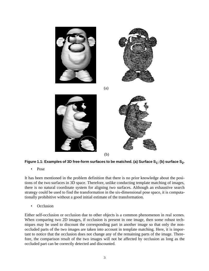
The two surfaces to be matched may have different topologies. For example, the two surfaces inFigure 1.1 are topologically different because they are two different surfaces, although they par-tially overlap. Occlusion can also result in topological difference. For example, in Figure 1.1, thecircled part onS2 appears to be a disconnected region due to occlusion. In contrast, its correspon-dence is connected to the entire surface onS1. The topology issue is difficult to address when try-ing to conduct global matching between two surfaces.

• Resolution

Generally speaking, the resolutions of different digitized surfaces are different. The resolutionproblem makes it difficult to establish the correspondences between two surfaces, which in turn,results in the difficulty of comparing the two surfaces. Even if the resolution of two sampled sur-faces is the same, in general, the sampling vertices on one surface are not exactly the same as thaton the other one.

• Connectivity

For arbitrary triangular meshes, the connectivities among vertices are arbitrary. Even if two sur-faces have the same number of vertices, they may still have different connectivities among verti-ces. This is in contrast to images. An image has a regularm by n matrix structure. Theconnectivities are the same for all the pixels (pixels on the boundary have the same connectivitypattern as well). When conducting template matching, the correspondences between two imagescan be naturally established.

3

• Pose

It has been mentioned in the problem definition that there is no prior knowledge about the posi-tions of the two surfaces in 3D space. Therefore, unlike conducting template matching of images,there is no natural coordinate system for aligning two surfaces. Although an exhaustive searchstrategy could be used to find the transformation in the six-dimensional pose space, it is computa-tionally prohibitive without a good initial estimate of the transformation.

• Occlusion

Either self-occlusion or occlusion due to other objects is a common phenomenon in real scenes.When comparing two 2D images, if occlusion is present in one image, then some robust tech-niques may be used to discount the corresponding part in another image so that only the non-occluded parts of the two images are taken into account in template matching. Here, it is impor-tant to notice that the occlusion does not change any of the remaining parts of the image. There-fore, the comparison result of the two images will not be affected by occlusion as long as theoccluded part can be correctly detected and discounted.

Figure 1.1: Examples of 3D free-form surfaces to be matched. (a) Surface S 1; (b) surface S 2.

(a)

(b)

4

In contrast to comparing 2D images, matching 3D free-form surfaces is far more complicatedwhen occlusion is present in the scene. Model-based matching is a common framework for solv-ing the 3D surface matching problem. It requires that an intermediate representation be created foreach given surface so that the problem of matching surfaces can be reduced to matching thoserepresentations. When there is occlusion in a given surface, it is important for the representationto remain the same as that created for the same surface without occlusion. Otherwise, the compar-ison of the two representations with and without occlusion will yield different results. Therefore,it is crucial for representations to be invariant to occlusion. However, this requirement is toodemanding to be fulfilled in practice. As an alternative, the representation is desired to changegradually as occlusion increases so that, the matching result degrades gracefully. Although a con-siderable amount of work has been done in developing representations for 3D free-form surfaces,the problem of developing occlusion-robust representation is still open.

1.3 Previous work

A considerable amount of research has been conducted on comparing 3D free-form surfaces. Theapproaches used to solve the problem can be classified into two categories according to methodol-ogy. Approaches in the first category try to create some form of representation for input surfacesand transform the problem of comparing the input surfaces to the simplified problem of compar-ing their representations. These approaches are used most often in model-based object recogni-tion. In contrast, approaches in the second category work on the input surface data directlywithout creating any kind of representation. One data set is aligned to the other by looking for thebest rigid transformation, using optimization techniques to search the six-dimensional pose space.These approaches are mainly used for surface registration.

According to the manner of representing the shape of an object, existing representations of 3Dfree-form objects may be regarded as either global or local. Examples of global representationsare algebraic polynomials[49][80], spherical representations such as EGI (extended GaussianImage)[40], SAI (Spherical Attribute Image)[34][36][19][20] and COSMOS (Curvedness-Orien-tation-Shape Map On Sphere)[25], triangles and crease angle histograms[9], and HOT (HighOrder Tangent) curves[47]. Although global representations can describe the overall shape of anobject, they have difficulties in representing objects of arbitrary topology or arbitrary complexityin shape. For example, the SAI can represent only objects with spherical topology. Moreover, glo-bal representations have difficulty in handling clutter and occlusion in the scene.

Many local representations are primitive-based. In [29], model surfaces are approximated by lin-ear primitives such as points, lines and planes. The recognition of objects is carried out byattempting to locate the objects through a hypothesize-and-test process. In [78], super-segmentsand splashes are proposed to represent 3D curves and surface patches with significant structuralchanges. A splash is a local Gaussian map describing the distribution of surface normals along ageodesic circle. Since a splash can be represented as a 3D curve, it is approximated by multipleline fitting with differing tolerances. Therefore, the splashes of the models can be encoded andstored in the database. The on-line matching of a scene object to potential model objects consistsof indexing into the database using the encoded descriptions of the scene splash to find the bestmatched model splash. In [16], a three-point-based representation is proposed to register 3D sur-faces and recognize objects in cluttered scenes. On the scene object, three points are selected withthe requirement that (1) their curvature values can be reliably computed; (2) they are not umbili-

5

cal points; and (3) the points are spatially separated as much as possible. Then, under the curva-ture, distance, and direction constraints, different sets of three points on the model surface arefound to correspond to three points on the scene objects. The transformations computed usingthose scene-model correspondences are verified to select the best one. More recently, a local rep-resentation called Spin-Images is proposed in [44]. Instead of looking for primitives or featurepoints at some parts of the object surface with significant structural changes, a Spin-Image is cre-ated for every point of the object surface as a 2D description of the local shape at that point. Givenan oriented point on the surface and its neighborhood of a certain size, the normal vector and thetangent plane are computed at that point. Then the shape of the neighborhood is described by therelative positions of the vertices in the neighborhood to the central vertex using the distances tothe normal and tangent plane. A Spin-Image is a 2D histogram of those distances. Good recogni-tion results in complex scenes using Spin-Images are reported in [44]. However, Spin-Images arenot well-understood at a mathematical level and they discard one dimension information of theunderlying surfaces, namely, Spin-Images do not preserve the continuity of surfaces. As can beseen from above, although local representations can not provide an overall description of theobject shape, they have advantages in handling clutter and occlusion in the scene.

Among 3D surface registration algorithms, Iterative Closest Point (ICP) plays an important role.In [10], the scene surface is registered with the model surface by iteratively finding the closestpoints on the model surface to the points on the scene surface and refining the transformation inthe six-dimensional pose space. Although this approach guarantees finding the local minimum ofthe registration error, it requires good initial estimate of the transformation in order to find theglobal minimum. Another limitation of this approach is that it can not handle two surfaces whichonly partially overlap. An heuristic method was proposed in [100] to overcome the partially over-lapping difficulty. A K-D tree structure was also used in [100] to speed up the process of findingthe closest point. Unlike the ICP approach, an algorithm is proposed in [14] to increase the accu-racy of registration by minimizing the distance from the scene surface to the nearest tangent planeapproximating the model surface. In order to reduce computational complexity, control points areselected for registration instead of using the entire data set of the model surface. However, thismay not work well on surfaces with no control points selected on some of their parts that have sig-nificant structural changes. Moreover, this approach also requires a good initial estimate of thetransformation. In [6], surfaces are approximated by constructing a hierarchy of Delaunay trian-gulations at different resolutions. Starting at a lower resolution, the correspondences between tri-angles can be established through the attributes of the triangles such as centroids and normals.Based on these correspondences, a rigid transformation can be computed and refined by trackingthe best matching pairs of triangles in the triangulation hierarchy. Although this algorithm wasproposed for integrating object surfaces from different view points, it can be modified and appliedto object recognition as well. In summary, in order for the surface registration algorithms to workwell, a good initial estimate of the transformation is usually required.

6

1.4 The Concept of Harmonic Shape Images

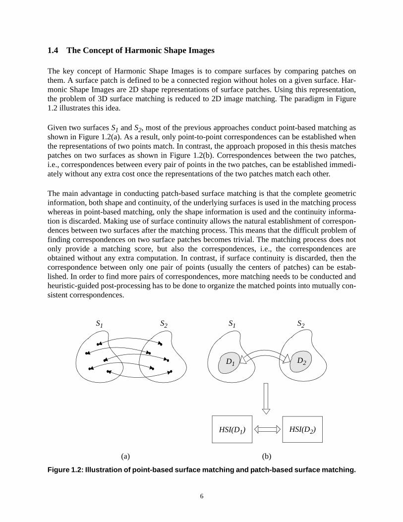
The key concept of Harmonic Shape Images is to compare surfaces by comparing patches onthem. A surface patch is defined to be a connected region without holes on a given surface. Har-monic Shape Images are 2D shape representations of surface patches. Using this representation,the problem of 3D surface matching is reduced to 2D image matching. The paradigm in Figure1.2 illustrates this idea.

Given two surfacesS1 andS2, most of the previous approaches conduct point-based matching asshown in Figure 1.2(a). As a result, only point-to-point correspondences can be established whenthe representations of two points match. In contrast, the approach proposed in this thesis matchespatches on two surfaces as shown in Figure 1.2(b). Correspondences between the two patches,i.e., correspondences between every pair of points in the two patches, can be established immedi-ately without any extra cost once the representations of the two patches match each other.

The main advantage in conducting patch-based surface matching is that the complete geometricinformation, both shape and continuity, of the underlying surfaces is used in the matching processwhereas in point-based matching, only the shape information is used and the continuity informa-tion is discarded. Making use of surface continuity allows the natural establishment of correspon-dences between two surfaces after the matching process. This means that the difficult problem offinding correspondences on two surface patches becomes trivial. The matching process does notonly provide a matching score, but also the correspondences, i.e., the correspondences areobtained without any extra computation. In contrast, if surface continuity is discarded, then thecorrespondence between only one pair of points (usually the centers of patches) can be estab-lished. In order to find more pairs of correspondences, more matching needs to be conducted andheuristic-guided post-processing has to be done to organize the matched points into mutually con-sistent correspondences.

Figure 1.2: Illustration of point-based surface matching and patch-based surface matching.

S1 S2 S1 S2

D1 D2

HSI(D1) HSI(D2)

(a) (b)

7

This thesis describes patch-based surface matching conducted by matching Harmonic ShapeImages of those patches as shown in Figure 1.2(b). Therefore, creating those images is the core ofthe patch-based matching. The main challenges for creating such a representation are as follows.The first one is that the representation needs to preserve both shape and continuity of the underly-ing surface patch. Previous approaches have shown that it is relatively easy to preserve shape onlybut not both. The second challenge is how to make the representation robust with respect to occlu-sion.

The following section introduces the generation of Harmonic Shape Images, discusses how toaddress the above two challenges, then summarizes the properties of Harmonic Shape Images.

Generation of Harmonic Shape Images

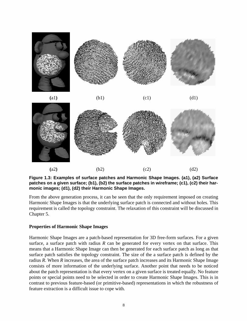
Given a 3D surfaceSas shown in Figure 1.3(a1), letv denote an arbitrary vertex onS. Let D(v, R)denote the surface patch which has the central vertexv and radiusR. R is measured by distancealong the surface.D(v, R) is assumed to be a connected region without holes.D(v, R)consists ofall the vertices inS whose surface distances are less than, or equal to,R. The overlaid region inFigure 1.3(a1) is an example ofD(v, R). Its amplified version is shown in Figure 1.3(b1). The unitdiscP on a 2D plane is selected to be the target domain.D(v, R)is mapped ontoP by minimizingan energy functional. The resultant imageHI(D(v, R)) is called the harmonic image ofD(v, R)asshown in Figure 1.3(c1).

As can be seen in Figure 1.3(a1) and (c1), for every vertex on the original surface patchD(v, R),one, and only one, vertex corresponds to it in the harmonic imageHI(D(v, R)). Furthermore, theconnectivities among the vertices inHI(D(v, R)) are the same as that ofD(v, R). This means thatthe continuity ofD(v, R)is preserved on the harmonic imageHI(D(v, R)).

The preservation of the shape ofD(v, R) is shown more clearly on the Harmonic Shape ImageHSI(D(v, R))(Figure 1.3(d1)) which is generated by associating shape descriptor at every vertexon the harmonic image(c1). The shape descriptor is computed at every vertex on the original sur-face patch(b1). OnHSI(D(v, R)), high intensity values represent high curvature values and lowintensity values represent low curvature values. The reason for Harmonic Shape Images’ ability topreserve the shape of the underlying surface patches lies in the energy functional which is used toconstruct the mapping between a surface patchD(v, R)and the 2D target domainP. This energyfunctional is defined to be the shape distortion when mappingD(v, R)ontoP. Therefore, by mini-mizing the functional, the shape ofD(v, R)is maximally preserved onP.

Another surface patch is shown in Figure 1.3(a2) and (b2). Its harmonic image and HarmonicShape Image are shown in (c2) and (d2), respectively. In this case, there is occlusion in the surfacepatch(Figure 1.3(b2)). The occlusion is captured by its harmonic image and Harmonic ShapeImage(Figure 1.3(c2), (d2)). The latter’s ability to handle occlusion comes from the way theboundary mapping is constructed when mapping the boundary ofD(v, R)onto the boundary ofP;because of the boundary mapping, the images remain approximately the same in the presence ofocclusion.

8

From the above generation process, it can be seen that the only requirement imposed on creatingHarmonic Shape Images is that the underlying surface patch is connected and without holes. Thisrequirement is called the topology constraint. The relaxation of this constraint will be discussed inChapter 5.

Properties of Harmonic Shape Images

Harmonic Shape Images are a patch-based representation for 3D free-form surfaces. For a givensurface, a surface patch with radiusR can be generated for every vertex on that surface. Thismeans that a Harmonic Shape Image can then be generated for each surface patch as long as thatsurface patch satisfies the topology constraint. The size of the a surface patch is defined by theradiusR. WhenR increases, the area of the surface patch increases and its Harmonic Shape Imageconsists of more information of the underlying surface. Another point that needs to be noticedabout the patch representation is that every vertex on a given surface is treated equally. No featurepoints or special points need to be selected in order to create Harmonic Shape Images. This is incontrast to previous feature-based (or primitive-based) representations in which the robustness offeature extraction is a difficult issue to cope with.

Figure 1.3: Examples of surface patches and Harmonic Shape Images. (a1), (a2) Surfacepatches on a given surface; (b1), (b2) the surface patches in wireframe; (c1), (c2) their har-monic images; (d1), (d2) their Harmonic Shape Images.

(a1) (b1) (c1) (d1)

(a2) (b2) (c2) (d2)

9

Harmonic Shape Images are defined on a simple domain which is a unit disc. This simplifies the3D surface matching problem to a 2D image matching problem. Furthermore, because the unitdisc is specified as the domain for any given surface patches, the Harmonic Shape Images of allthose patches are defined in the same coordinate system regardless of the actual positions of thosepatches. This means that Harmonic Shape Images are pose invariant.

Harmonic Shape Images capture both the shape and the continuity information of the underlyingsurface patches. It can be seen easily from Figure 1.3 that there is one-to-one correspondencebetween the vertices on the surface patch and its harmonic image. In fact, the mapping from thesurface patch to the disc domain is a well-behaved mapping. It is one-to-one and onto; it is contin-uous; it is unique; and it is intrinsic to the original surface patch. This property allows the naturalestablishment of correspondences between two surface patches once their Harmonic ShapeImages match.

Finally, Harmonic Shape Images are robust to occlusion and sampling resolution. This propertyhas been briefly discussed earlier in this section and will be discussed in detail in later chapters.

The comparison of Harmonic Shape Images and some surface representations previously pro-posed is listed in Table 1.1.

1.5 Thesis Overview

This thesis presents a novel representation, Harmonic Shape Images, for 3D free-form surfaces. Inaddition to describing in detail the generation of Harmonic Shape Images, the properties of thisrepresentation are thoroughly investigated by conducting various experiments. A surface match-ing strategy using Harmonic Shape Images is proposed and applied to surface matching experi-ments. The usefulness of these images is demonstrated by different applications of surfacematching. There are eight chapters in this thesis. The content of each chapter is summarized asfollows.

Chapter 2 describes the generation of Harmonic Shape Images in detail. The concepts of 3D sur-face patch and 2D target domain are first defined followed by the two-step construction of theharmonic map. The interior mapping and boundary mapping are the crucial steps in constructingthe harmonic map between a 3D surface patch and the 2D target domain. The generation of Har-monic Shape Images is then discussed as a surface attribute association process on the harmonicmaps.

Chapter 3 discusses the matching of Harmonic Shape Images. A shape similarity measure of theseimages is defined and a statistical approach is presented for quantitatively determining how a Har-monic Shape Image differs from others. At the end of Chapter 3, a 3D free-form surface-matchingstrategy using Harmonic Shape Images is presented.

In Chapter 4, an experimental approach is employed to analyze and demonstrate some of theimportant properties of Harmonic Shape Images. Those properties include discriminability, sta-bility, robustness to surface sampling resolution and robustness to occlusion. Two libraries of sur-face patches are used in those experiments.

10

Chapter 5 discusses some enhancements for Harmonic Shape Images. The hole interpolationstrategy can help relax the topology constraint which has been discussed earlier in this Chapter.The cutting and smoothing techniques can further improve the robustness of Harmonic ShapeImages in the presence of occlusion.

In Chapter 6, experiments on surface matching using Harmonic Shape Images are described andthe results are presented and analyzed. Application examples of surface matching include facemodeling and mesh watermarking. Harmonic Shape Images have also been used to recognizeobjects in scenes with occlusion. Experiments have been conducted to measure the registrationerror using Harmonic Shape Images.

Chapter 7 discusses the future research directions for the use of Harmonic Shape Images. Someextensions can be added to the images to improve the matching process. Applications of theimages in Shape analysis are discussed.

Chapter 8 concludes this thesis by summarizing the contributions of the thesis.

Table 1.1 Comparison of some surface representations

ComparisonItems

Repre-sentations

Objectdomain

Type ofrepresentation

MappingCompleteness

ofrepresentation

SAI Objects withsphericaltopology

Global Spherical mapping ofsurface curvature atall points

Complete, bothsurface shapeand continuityare represented

Splashes Objects with-Free-formsurfaces

Local Gaussian map of sur-face normals along ageodesic circle

Partial

COSMOS Objects with-Free-formsurfaces

Global Spherical mapping oforientation ofCSMPs

Partial for non-convex objects

Spin-Images Objects with-Free-formsurfaces

Local 2D histogram of dis-tances to the refer-ence tangent planeand surface normal atall points

Partial, surfacecontinuity is notrepresented

HSI Objects with-Free-formsurfaces

Local Harmonic map of theunderlying surfaceonto a unit disc. sur-face curvature isstored on the map forall points.

Complete, bothsurface shapeand the continu-ity are repre-sented

11

Chapter 2

Generating Harmonic Shape Images

The name of Harmonic Shape Images comes from the fact that the mathematical tool, whichis called harmonic maps, is used in its generation process. The idea of using harmonic maps todevelop a surface representation is partly inspired by the work in the computer graphics fielddone by Eck et al.[26] at the University of Washington.

Given a triangular meshS with arbitrary topology, the goal of the work in [26] is to create aremesh S’which has the same shape asSbut the connectivities among its vertices satisfy a subdi-vision requirement[26]. As part of the remeshing process,S is partitioned into connected surfacepatches without holes and each such patch is mapped onto an equilateral triangle using harmonicmaps. The maps on those equlateral triangles are then used to resampleSwith specified connec-tivities among the resampled points. It can be seen that the use of harmonic maps in [26] is to per-form a certain form of resampling on 3D triangular meshes.

In this thesis, the use of harmonic maps is to conduct surface matching which is different fromthe goal in [26]. In order to compare two surfaces, an intermediate representation, HarmonicShape Images, is created using harmonic maps. The concept of Harmonic Shape Images has beenintroduced in Chapter 1. In this chapter, the generation of Harmonic Shape Images will be dis-cussed in detail. The background of Harmonic Maps is briefly reviewed first. The source and tar-get manifolds in creating Harmonic Shape Images are then defined. The core steps of thegeneration process, the interior mapping and the boundary mapping, are explained next in detailfollowed by the discussion on how to select the parameters when generating Harmonic ShapeImages. At the end of this chapter, different schemes for approximating the curvature at each ver-tex of the surface mesh are presented.

2.1 Harmonic Maps

The theory of Harmonic Maps studies the mapping between two manifolds from an energypoint of view. Formally, let(M, g) and (N, h) be two smooth manifolds of dimensionsm andnrespectively, and letφ: be a smooth map. Let (xi), and (yα)

be local coordinates aroundx and φ(x), respectively. Take (xi) and (yα) of M andN at corresponding points under the mapφ whose tangent vectors of the coordinate curves are

and , respectively. Then the energy density ofφ is defined as[94]

(2.1)

In (2.1),gij andhαβ are the components of the metric tensors in the local coordinates onM andN,respectively. The energy ofφ in local coordinates is given by the number[94]

(2.2)

M g,( ) N h,( )→ i 1 … m, ,=α 1 … n, ,=

∂ ∂xi⁄ ∂ ∂y

α⁄

e φ( ) 12--- g

ij φ*x

i∂∂ φ*

xj∂

∂,ÿ þN

i j, 1=

m

12--- g

ij φα∂x

i∂--------- φβ∂

xj∂

--------hαβ φ( )α β, 1=

n

i j, 1=

m

==

E φ( ) e φ( )vgM=

12

If φ is of class C2, , andφ is an extremum of the energy, thenφ is called a harmonicmap and satisfies the corresponding Euler-Lagrange equation. In the special case in whichMis a surfaceD of disc topology andN is a convex regionP in E2, the following problem has aunique solution[27]: Fix a homeomorphismb between the boundary ofD and the boundary ofP.Then there is a unique harmonic mapφ: that agrees withb on the boundary ofD and min-imizes the energy functional ofD. In addition to the energy minimizing property, the harmonicmapφ has the following properties: it is infinitely differentiable; it is an embedding ofD into P; itis intrinsic to the underlying surface.

2.2 Definition of Surface Patch

The concept of surface patch has been explained briefly in Section 1.4. In this section, surfacepatch is defined formally as follows. Given a 3D free-form surfaceS represented by triangularmesh, an arbitrary vertexv on Sand a radiusR measured by surface distance, a surface patchD(v,R) of S is defined to be the neighborhood ofv, which includes all the vertices whose surface dis-tances tov are less than or equal toR. D(v, R) is said to be valid when the topology constraint,which requiresD(v, R) be connected and without holes, is satisfied. Three surface patches areshown in Figure 2.1(a), (b) and (c), respectively. Their wireframe versions are shown in Figure2.1(d), (e) and (f). The patch in Figure 2.1(a) is valid while the patches in Figure 2.1(b) and (c) areinvalid because they both have holes.

The implementation of generating a surface patch mainly involves the computation of theshortest path from a given vertex to any other vertex on the underlying triangular mesh. Thetriangular mesh can be considered as a bi-directional connected graph which has positive costfor all of its edges. Then the problem of computing the shortest path from a given vertex toany other vertex can be solved using the Single Source Dijkastra’s algorithm[1].

Two implementation issues that need to be discussed about generating surface patches arehow to deal with dangling triangles and how to use the radius margin.

Dangling Triangles

After a surface patch is generated, a post-processing step needs to be done in order to clean upthe patch boundary. The purpose of the cleanup is to delete the dangling triangles on the patchboundary. For example, the surface patch shown in Figure 2.2(a) has two dangling triangles(shaded). The reason for performing this operation is as follows. When constructing the boundarymapping which will be explained in the following section, the boundary vertices need to beordered in either a clock-wise or counter-clock-wise manner. In Figure 2.2(a), starting from vertexv1, it is not uniquely determined whether the next boundary vertex should bev2 or v4 becausethere is a loop caused by the dangling triangle(v2, v3, v4). Here, a triangle is considered to be dan-gling if not all of its three vertices have degrees greater than or equal to three. In order to uniquelydetermine the ordering of the boundary vertices and avoid boundary pathologies(Figure 2.2(b)),dangling triangles on surface patches such as the ones in Figure 2.2(a), (b) need to be pruned.

E φ( ) ∞<

D P→

13

Radius Margin

Another issue with generating surface patches is the radius margin. In general, the shortestdistance from a vertexu to the central vertexv can not be exactly equal to the specified radiusR. If the vertexu is not included in the surface patch centered atv because the shortest dis-tance fromu to v is slightly greater than the specified radiusR, then some information may belost due to the irregular sampling of the mesh as shown in Figure 2.3. In Figure 2.3(a) and (c), thetwo surfaces have the same shape but different sampling. If a surface patch is to be generated atvertexv using radiusR on the two surfaces shown in (a) and (c), respectively, then the resultantsurface patches are shown in (b) and (d), respectively. It can be seen that the vertexu is notincluded in the surface patch in (b) because the shortest distance fromu to v is slightly greaterthanR. In contrast,u is included in the surface patch shown in (d) because the shortest distancefrom u to v is equal toR. The difference in the shortest distance fromu to v is not caused by theshape of the surface. Rather, it is caused by the sampling noise. If a radius margin, which is equalto a small percentage ofR, is added to the actual radius, then the vertexu will be included in the

Figure 2.1: Example of surface patches. (a) A valid surface patch; (b), (c) Invalid surfacepatches; (d), (e), (f) Surface patches of (a), (b) and (c) in wireframe form, respectively.

(a) (b) (c)

(d) (e) (f)

14

surface patch in (b) and the resultant surface patch will be more similar to the one in (d). As asummary, using radius margin is a heuristic to overcome sampling noise when generating surfacepatches so that the surface patches to be compared would be as similar as possible if they wereactually the same patch. In all the experiments that have been conducted, the radius margin is setto be 5%.

It should be noted that the radius margin is only a computationally inexpensive heuristic toreduce the influence of the surface sampling noise. It is not a permanent fix for the problem.In fact, interpolation on the edges along with triangulation is a better solution, especially whenthe mesh resolution varies widely across the mesh. Figure 2.4 illustrates the idea of the interpola-tion and triangulation strategy. In Figure 2.4(a), the vertices marked by the gray dots are in thesurface patch while the vertexv1, marked by the white dot, is not. Interpolation is performed onthe edge connectingv1 andv5. This edge is on the shortest path fromv1 to the center of the surfacepatch.u1 is the resultant vertex of the interpolation. Local triangulation is performed after theinterpolation and four new triangles are created. The two lightly shaded triangles along with theheavily shaded triangles are in the surface patch.

When using the interpolation and triangulation strategy, the condition under which an edgeshould be split is that both vertices that the edge faces should be in the surface patch. If thiscondition is not satisfied, as shown in Figure 2.4(b), then no interpolation is performed along thatedge. In Figure 2.4(b), becausev2 is not in the surface patch, the edge connectingv1 andv5 is notsplit. In contrast, interpolation is performed along the edge connectingv2 andv6 and vertexu2 iscreated. The resultant surface patch contains the two lightly shaded triangles along with theheavily shaded ones.

Figure 2.2: Surface patches with dangling triangles on the boundary.

v1

v2

v3

v4

v1

v2

v3

v4

(a) (b)

15

Figure 2.3: Illustration of radius margin. (a), (c) Surfaces that have the same shape butdifferent sampling; (b) the surface patch generated using the center vertex v and radius Ron the surface in (a). Vertex u is not included in the patch because the shortest distancefrom u to v is slightly greater than R. If using the 5% radius margin, then vertex u will beincluded in the patch. The resultant patch is similar to the one in (d). (d) The surface patchgenerated using the center vertex v and radius R on the surface in (b). Vertex u is includedin the patch because the shortest distance from u to v is equal to R.

Figure 2.4: Illustration of the interpolation and triangulation strategy.

v

R R

u

v

v

RR

u

v

u

(a) (b)

(c) (d)

v1

v2 u1

v4

v1

v3

v5

v3

v5

v4

v2

(a) (b)

v6v6

v7v7u2

16

2.3 Interior Mapping

The theory of harmonic maps has been briefly reviewed in Section 2.1. It is clear that the solutionto harmonic maps is the solution to a partial differential equation. Because we deal with discretesurfaces in practice and the computation cost for solving partial differential equations is high, it ismore appropriate and practical if some approximation approaches can be used to compute har-monic maps. In [26], an approximation method is proposed; the method consists of two steps:interior mapping and boundary mapping. In our approach, we use an interior mapping which issimilar to that in [26], but a different boundary mapping. In this section, assuming that the bound-ary mapping is already known, the construction of the interior mapping is discussed in detail. Theboundary mapping will be discussed in Section 2.4.

Defining Energy Functional

Let D(v, R) be a 3D surface patch with central vertexv and radiusR measured by surface dis-tance. LetP be a unit disc in a two-dimensional plane. Let and be the boundary ofDand P, respectively. Let , be the interior vertices ofD. The interior mappingφmaps onto the interior of the unit discP with a given boundary mappingb:

. φ is obtained by minimizing the following energy functional[26]:

(2.3)

In (2.3), for the simplicity of notation,φ(i) andφ(j) are used to denote and which arethe images of the vertices and onP under the mappingφ. The values ofφ(i) andφ(j) definethe mappingφ. kij serve as spring constants which will be discussed shortly.

The intuition of the energy functional is as follows. An instance of the functional E(φ) can beinterpreted as the energy of a spring system by associating each edge inD with a spring. Thenthe mapping problem fromD to P can be considered as adjusting the lengths of those springswhen flattening them down ontoP. If the energy ofD is zero, then the energy increases whenthe mesh is flattened down toP because all the springs are deformed. Different ways ofadjusting the spring lengths correspond to different mappingsφ. The bestφ minimizes theenergy functional E(φ).

The minimum of the energy functional E(φ) can be found by solving a sparse linear least-square system of (2.3) for the valuesφ(i). Taking the partial derivative of E(φ) with respect toφ(i),

and making it equal to zero yield the following equations:

(2.4)

(2.5)

∂D ∂Pvi i, 1 … n, ,=

vi i, 1 … n, ,=∂D ∂P→

E φ( ) 12--- kij φ i( ) φ j( )–

2

i j, Edges D( )∈=

φ vi( ) φ vj( )vi vj

i 1 … n, ,=

∂E φ( )∂φ i( )--------------- kij φ i( ) φ j( )–( ) kik φ i( ) φ k( )–( ) kil φ i( ) φ l( )–( ) … i,+ + + 1 … n, ,= =

kij φ i( ) φ j( )–( )i j, 1 Ringof i –∈

= 0 i, 1 … n, ,= =

17

In (2.5),1-Ring of i, illustrated in Figure 2.5, refers to the polygon constructed by the immediateneighboring vertices of the vertexvi. Equation (2.5) can be rewritten as

(2.6)

In (2.6), , . denotes the unknown coordi-nates of the interior vertices ofD when mapped ontoP underφ. Because contains the con-nectivity information of the surface patchD(v, R), it is a sparse matrix that has the followingstructure (Figure 2.6). IfD is considered to be a bi-directional graph, then can be interpreted

as the adjacency matrix of the graph. All the diagonal entries of are non-zero. For an arbi-trary row i in , if vertex is connected to vertices and ,i.e., and are in the1-

Figure 2.5: Illustration of the 1-Ring of a vertex on a triangular mesh.

Figure 2.6: Structure of the matrix .

vi

vkvl

vm

vn

vo

vp

vqvj

AnxnXnx2 bnx2=

Xnx2 φ 1( ) … φ n( ), ,[ ]T= φ i( ) φx i( ) φy i( ),[ ]= Xnx2

Anxn

Anxn

i

*

m n

*

j

*

*

... ... ... ...1

*

*

*

i

m

n

j

......

......

1...

*

*

...

...

...

...

...

...

...

Anx n =

Anxn

AnxnAnxn vi vj vm vj vm

18

Ring of , then only thejth andmth entries in rowi are non-zero. Similarly, theith entry in rowm and rowj are also non-zero. Therefore, in addition to the usual properties that matrix hasin least-square problems, is sparse in this particular case. The boundary condition is accom-modated in the matrix . In , if a vertex is connected to boundary vertices, then itscorresponding entryi in is weighted by the coordinates of those boundary vertices. Other-wise, the entries in are zero.

Solving the Sparse Linear System

In our current implementation, (2.6) is solved using the conjugate gradient descent algorithm. Inaddition to the usual steps in implementing that algorithm, special attention is paid to the storageof the matrix in (2.6) because is a sparse matrix. Storing as an by n matrixwould waste a great deal of memory. In our current implementation, theindexed storagestrategyintroduced in [64] is adopted to store as two arrays with one being integer array and theother being double array. The index storage strategy is illustrated by the following example. Sup-pose that

(2.7)

In order to represent a sparse matrixAnxn like the one in (2.7) using the row-indexed scheme, twoone-dimensional arrays need to be set up. One is an integer array calledija and the other is a dou-ble array calledsa. The following rules are applied to created the two arrays:

• The firstN locations ofsastoreA’s diagonal matrix elements in order.

• Each of the firstN locations ofija stores the index of the arraysa that contains the firstoff-diagonal element of the corresponding row of the matrix. If there are no off-diago-nal elements for that row, it is one greater than the index insa of the most recentlystored element of a previous row.

• Location 1 ofija is always equal toN+2 which can be read to determineN.

• Location N+1 of ija is one greater than the index insa of the last off-diagonal elementof the last row. It can be read to determine the number of nonzero elements in thematrix, or the number of elements in the arrayssa and ija. Location N+1 of sa is notused and can be set arbitrarily.

• Entries in sa at locations containAnxn’s off-diagonal values, ordered byrows and, within each row, ordered by columns.

• Entries in ija at locations contain the column number of the correspondingelements insa.

viAnxn

Anxnbnx2 Xnx2 vi

bnx2bnx2

Anxn Anxn Anxn

Anxn

A

3 0 1 0 0

0 4 0 0 0

0 7 5 9 0

0 0 0 0 2

0 0 0 6 5

=

N 2+≥

N 2+≥

19

Using the above rules to construct the indexed storage arrays for the matrix A in (2.7) yields theresult shown in Figure 2.7. In that figure, it should be noticed that, according to the above storage

rules, the value ofN (namely 5 in this case) isija[1]-2, and the length of each array isija[ija[1]-1]-1, namely 11. The first five elements insaare the diagonal values of A in order. The 6th valueis x, which represents an arbitrary value. The elements numbered from 7 to 11 insa are the off-diagonal entries of each row inA. For each rowi in A, the off-diagonal elements are stored insa[k] wherek loops fromija[i] to ija[i+1]-1. For example, let us find the off-diagonal elements inthe first row of A in (2.7). From the index inija[1] and ija[2], it can be determined that there isone off-diagonal element in that row. The value of this element is located insa[ija[1]], i.e., sa[7],which is equal to 1.0. The column index of this element in the original matrixA is located inija[ija[1]], i.e., ija[7], which is 3. Checking the original matrixA will verify the results we justobtained.

Defining Spring Constants

There are different ways of assigning the spring constants in (2.3). One is to define the spring con-stant as in (2.8)[26]

(2.8)

in which and are defined in Figure 2.8.

Figure 2.7: The row-indexed storage arrays for the matrix in (2.7).

Figure 2.8: Definition of spring constants using angles.

indexk 1 2 3 4 5 6 7 8 9 10 11

ija[k] 7 8 8 10 11 12 3 2 4 5 4

sa[k] 3.0 4.0 5.0 0.0 5.0 x 1.0 7.0 9.0 2.0 6.0

kij ctgθ emi emj,( ) ctgθ eli elj,( )+=

θ emi emj,( ) θ eli elj,( )

vi

vj

vlvm

emi eli

emj elj

eijθ(emi, emj) θ(eli , elj)

20

If eij is associated with only one triangle, then there will be only one term on the right-hand side of(2.8). The intuition behind this definition is that long edges subtending to big angles are given rel-atively small spring constants compared with short edges which subtend to small angles. Recallthe energy functional defined in (2.3); this definition of the spring constant means that long edgeswill remain long in the harmonic image while short edges will remain short. The reason is that thesprings associated with long edges have smaller spring constants compared with the springs asso-ciated with short edges. Figure 2.9 shows an example of the interior mapping.: a hemisphere rep-

resented by triangular mesh. It should be noted that most of the vertices are distributed evenly onthe mesh except at the parts indicated by arrows. In other words, most of the edges have equallength on the mesh. The harmonic image of the mesh is shown in Figure 2.9(b). The short edgesindicated in Figure 2.9(a) by arrows are still short in (b) while other edges in (a) remain long in (b)and they have approximated equal length locally. There is obvious boundary distortion on the har-monic image due to the discrete nature of the triangular mesh. The distortion affects the interiormapping; therefore, most of the edges in (b) do not have equal length as they do in (a). Figure 2.10shows the harmonic image of a surface patch from a real object.

From the above discussion, it can be seen that the energy functional in (2.3) tries to preserve theratio of edge lengths on the original surface patchD(v, R) by defining the spring constants asshown in (2.8). Given a specific sampling of a surface (a surface can be sampled in differentways), the ratio of edge lengths is closely related to the shape of the surface. Therefore, by pre-serving the ratio of edge lengths, the interior mappingφ preserves the shape of theD(v, R)whenmapping it onto the unit discP. Of course there is distortion when mappingD(v, R)onto P. Thedistortion is minimized byφ.

In order to preserve the ratio of edge lengths, another way to define the spring constant is touse the inverse of the edge length as shown in (2.9).

Figure 2.9: Example of interior mapping. (a) A hemisphere represented by triangularmesh; (b) the harmonic image of (a).

(a) (b)

21

(2.9)

Similar to (2.8), the springs associated with longs edges have small spring constants while thesprings associated with short edges have large spring constants. Using the definition in (2.9), theinterior mappings for the surfaces shown in Figure 2.9(a) and Figure 2.10(a) are computed andshown in Figure 2.11.

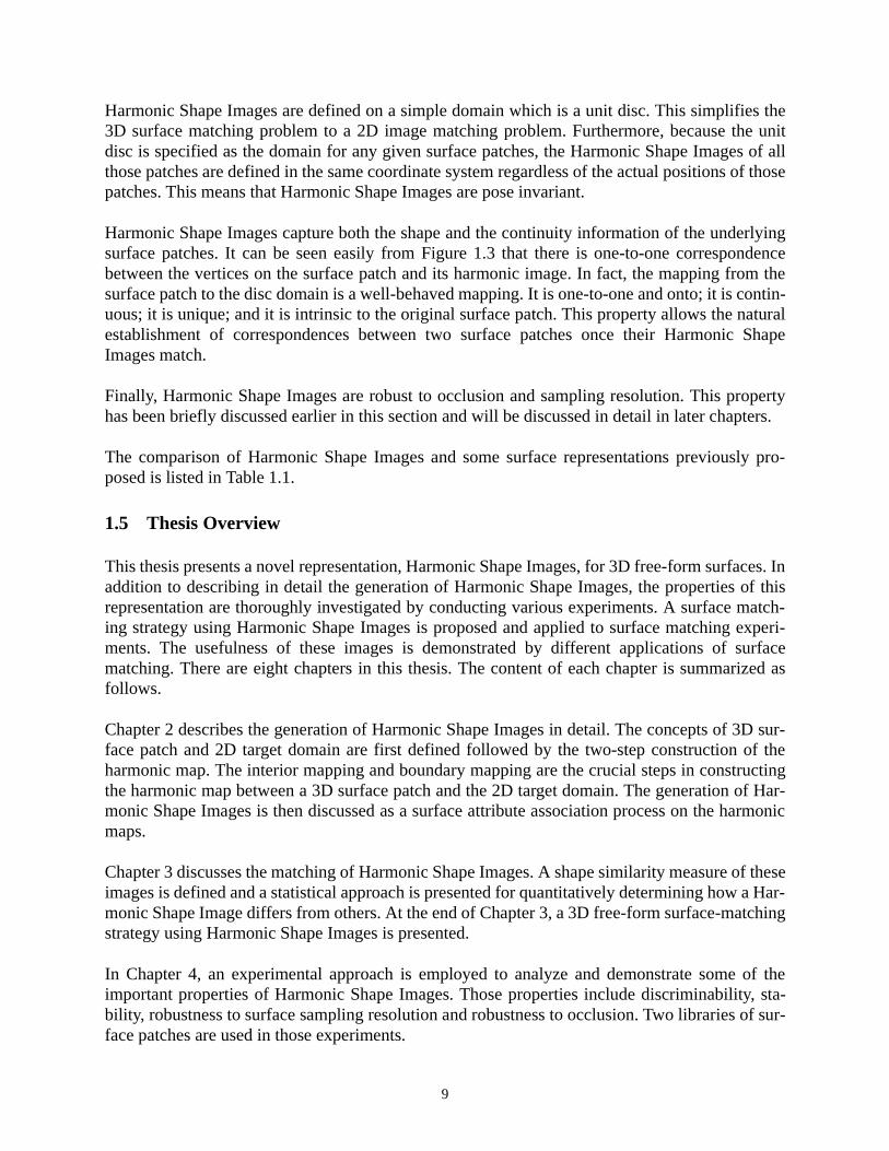
Figure 2.10: An example of the interior mapping using a real object. (a) Original surfacepatch (rendered); (b) original surface patch shown in wireframe; (c) the harmonic image of(b).

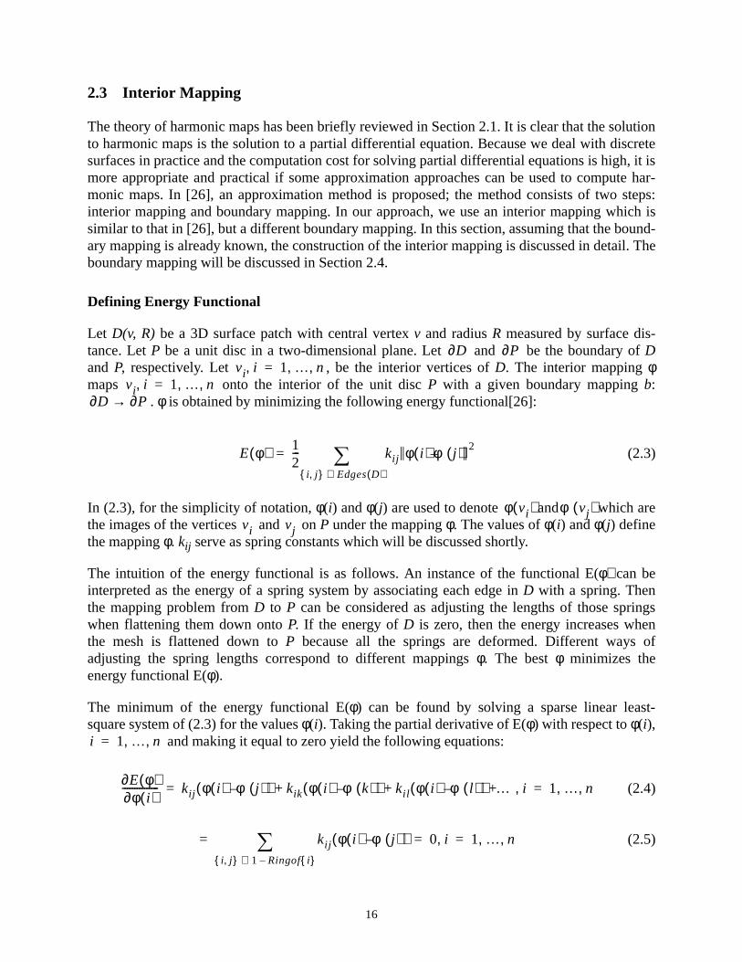
Figure 2.11: Harmonic images computed using the inverse of edge length as springconstant. (a) Harmonic image of the hemisphere shown in Figure 2.9(a); (b) harmonic im-age of the surface shown in Figure 2.10(a).

(a) (b) (c)

kij1

evi vj

-------------=

(a) (b)

22

According to the experiments that have been conducted, there is little difference between theharmonic images resulted from the two approaches to defining the spring constants. Forexample, the harmonic images in Figure 2.9(b) and Figure 2.11(a) are almost the same. So are theimages in Figure 2.10(c) and Figure 2.11(b). For the second case, for each vertex on the two har-monic images, the length of the difference vector is plotted in Figure 2.13. The curve shows thatlittle variation in postion for each vertex on the harmonic images results from using differentdefinitons of the spring constant. The unit of the vertical axis in Figure 2.13 is the radius of the 2Dunit disc.

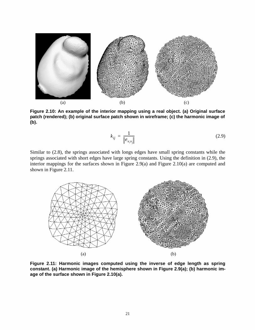
When the ratio of edge length varies significantly across the surface patch (Figure 2.12(b)), thedifference between the harmonic images obtained using different definitions of spring constants ismore visible (Figure 2.12(c) and (d)). The length of the difference vector for each vertex is plottedin Figure 2.14. However, even in this case, there is little effect on the Harmonic Shape Imageswhich are created based on harmonic maps. Harmonic Shape Images will be discussed in Section2.5.

As a summary, based on the experiments we have conducted, no evidence has been found toshow that one definition is better than the other. The angle definition is used in all experi-ments.

2.4 Boundary Mapping

As discussed in Section 2.3, the unit discP is selected to be the target domain of the harmonicmapping. In this section, the construction of boundary mapping, which maps the boundary of thegiven surface patchD(v, R)onto the boundary ofP is discussed.

The construction of the boundary mapping is illustrated in Figure 2.15. First of all, let us definethe vertices and vectors in Figure 2.15.O is the central vertex of the surface patchD(O, R)andO'is the center of the unit discP. vi, i=1,…,5 are the boundary vertices ofD(O, R). For some bound-ary vertices, e.g.,vi

r, i=1,…,4, the surface distance between any of them and the central vertexOis equal toR; these are calledradius boundary vertices. For other boundary vertices, e.g.,v1

o, thesurface distance is less thanR; these are calledoccluded boundary vertices. Radius boundary ver-tices are determined by the radius of the surface patch, while occluded boundary vertices aredetermined either by self occlusion or by occlusion by other objects. The vector from the centralvertexO to a radius vertexvi

r is called aradius vector, while the vector fromO to an occludedboundary vertexvj

o is called anocclusion vector.

Now let us define the angles in Figure 2.15. Anglesai, i=1,…,4 are the angles between two adja-cent radius vectorsvi

rO andvi+1rO. Anglesbj, j=1, 2, are the angles between two adjacent occlu-

sion vectors, or one occlusion vector and one adjacent radius vector, in an occlusion range. Anocclusion range is a consecutive sequence of occlusion boundary vertices except for the first andlast ones. For example, (v4

r, v1o, v1

r) is an occlusion sequence. The sum ofbj over an occlusionsequence is the angleai formed by the first and last radius vectors, for example, the sum ofbj over(v4

r, v1o, v1

r) is a1.

23

Figure 2.12: An example mesh with large variation of the ratio of edge lengths. (a) Renderedsurface; (b) surface in wireframe; (c) harmonic image using the angle definition; (d) har-monic image using the inverse of edge length definition.

(a) (b)

(c) (d)

24

Figure 2.13: The position difference for each vertex on the two harmonic images ob-tained using different definitions of the spring constant. The original surface patch isshown in Figure 2.10(a). Harmonic images are defined on the 2D unit disc. The unit of thevertical axis is the radius of the 2D unit disc.

Figure 2.14: The position difference for each vertex on the two harmonic images ob-tained using different definitions of the spring constant. The original surface patch isshown in Figure 2.12(a). Harmonic images are defined on the 2D unit disc. The unit of thevertical axis is the radius of the 2D unit disc.

25

The construction of the boundary mapping consists of two steps. At the first step, the radiusboundary vertices are mapped onto the boundary of the unit discP, which is a unit circle. In Fig-ure 2.15,vi

r, i=1,…,4, are mapped tovir', i=1,…,4, respectively. Once the anglesai are deter-

mined, the positions ofvir' are determined.θi is computed as follows:

(2.10)

At the second step, the occlusion boundary vertices in each occlusion range are mapped ontothe interior of the unit discP. For example, in Figure 2.15,v1

o, which is in the occlusion range(v4

r, v1o, v1

r), is mapped ontov1o'. Once the anglesψj and the radiirj are determined, the position

of v1o is determined.ψj are computed as follows.

(2.11)

in which n is the number of angles within the occlusion range. The sum in the denominator isequal to the angle formed by the first and last radius vectors of the occlusion range. In Figure2.15, it is equal toa1. rj is defined to be

Figure 2.15: Illustration of the boundary mapping.

v2r

v3r v4

r

v1r

v1o

v2r’

v3r’

v4r’

v1r’

v1o’

a2

a3 a4

b1

b2 a1

ψ1

θ3

θ4 ψ2

θ2

θ1

O O’

D Pb

θi

ai

ak

k 1=

n

---------------2π=

ψj

bj

bm

m 1=

n

------------------=

26

(2.12)

in which dist(vjo, O) is the surface distance between the occlusion boundary vertexvj

o and thecentral vertexO. R is the radius of the surface patchD(O, R).

The intuition behind the boundary mapping is that the ratio of the boundary edge lengths ispreserved as much as possible on the boundary ofP. This is consistent with the way the inte-rior mapping is constructed. Therefore, the harmonic mapping minimizes the shape distorsionwhen mapping the surface patchD(v, R)onto the 2D unit discP.

In the following sections, we discuss ordering the boundary vertices and selecting a startingboundary vertex.

Ordering Boundary Vertices

The boundary vertices ofD need to be ordered in either a clock-wise or counter-clock-wisemanner before constructing the boundary mapping. Similarly, when mapping vertices onto theboundary ofP, either clock-wise or counter-clock-wise order needs to be determined. To facil-itate matching, the two orders must remain consistent for all surface patches. In our imple-mentation, a vector is assumed to be known as the reference vector for a given surface patch.The viewing direction along which the range image of the surface patch is taken can be usedas the reference vector. The order of the boundary vertices is determined according to thisvector.

Selecting Starting Boundary Vertex

When constructing the boundary mapping, if the starting vertex on the boundary ofD isalways mapped to the same vertex on the boundary ofP, then different starting vertices willresult in different boundary mappings. This will, in turn, result in different interior mappings.For example, a surface patch is shown in Figure 2.16(a) and (b). With different starting verticesindicated by the arrow, two different harmonic images are obtained (Figure 2.16(c) and (d)).

A closer examination on the harmonic images in Figure 2.16(c) and (d) shows that one image isthe rotated version of the other. In fact, the harmonic images with different starting vertices aredifferent by a planar rotation because neither the anglesθi in (2.10) nor the anglesψi in (2.11)change with respect to different starting vertices. Nor does the radiusrj in (2.12) change. There-fore, the starting vertex can be selected randomly. The rotation difference will be found later bythe matching process which will be discussed in the next chapter.

2.5 Generation of Harmonic Shape Images

In Sections 2.2, 2.3 and 2.4, we have discussed defining a surface patch and obtaining its har-monic image. In this section, we will explain how to construct its Harmonic Shape Image from itsharmonic image.

r j

dist vjo

O,( )R

---------------------------=

27

Recall from previous sections that one important property of harmonic images is the one-to-one correspondence between the vertices on the surface patchD(v, R) and those on its har-monic imageHI(D(v, R)). This means that, all distribution functions defined on a surfacepatch can be recorded accordingly on its harmonic image. In other words, harmonic imagesprovide a general framework for representing distribution functions defined on surfaces, e.g.,surface normal, shape, color, texture, material. To describe the shape of free-form surfaces,the shape information, e.g., curvature, is stored at each vertex of the harmonic imageHI(D(v,R)). The resultant image is called a Harmonic Shape Image, which is denoted asHSI(D(v, R)).If texture information is stored onHI(D(v, R)), the resultant image is called a Harmonic Tex-ture Image.

Curvature is the shape descriptor of surfaces. However, there are two difficulties in computingcurvature in practice. One is that we deal with discrete surfaces. The other is that computingcurvature involves computing the second order derivatives, which are sensitive to noise. Oneway to address these issues is that smooth surfaces can be fit to the triangular mesh locally so

Figure 2.16: The effect of starting vertex on harmonic images. (a) A surface patch (ren-dered); (b) the wireframe version of (a). It is displayed from a different viewing directionfrom that in (a) in order to show the shape of the surface patch clearly. (c) The harmonicimage of (a) with the starting vertex indicated by the arrow; (d) the harmonic image of (a)with a different starting vertex indicated by the arrow.

(a) (b)

(c) (d)

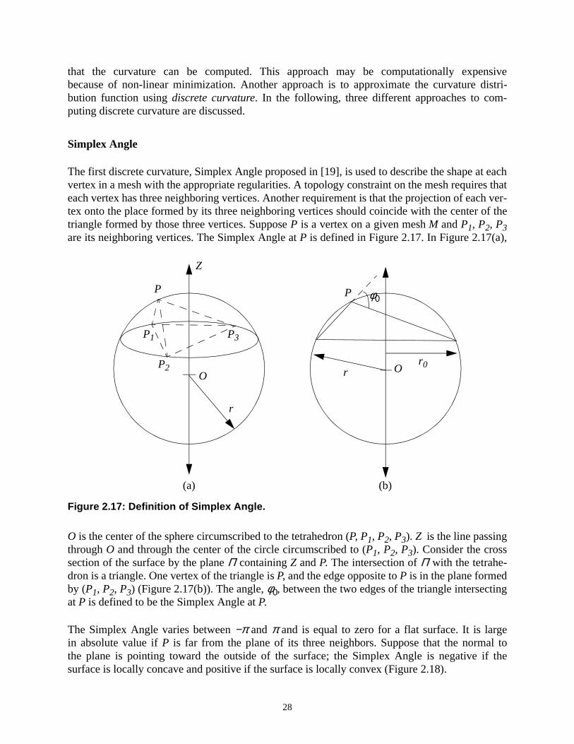
28

that the curvature can be computed. This approach may be computationally expensivebecause of non-linear minimization. Another approach is to approximate the curvature distri-bution function usingdiscrete curvature. In the following, three different approaches to com-puting discrete curvature are discussed.

Simplex Angle

The first discrete curvature, Simplex Angle proposed in [19], is used to describe the shape at eachvertex in a mesh with the appropriate regularities. A topology constraint on the mesh requires thateach vertex has three neighboring vertices. Another requirement is that the projection of each ver-tex onto the place formed by its three neighboring vertices should coincide with the center of thetriangle formed by those three vertices. SupposeP is a vertex on a given meshM andP1, P2, P3are its neighboring vertices. The Simplex Angle atP is defined in Figure 2.17. In Figure 2.17(a),

O is the center of the sphere circumscribed to the tetrahedron (P, P1, P2, P3). Z is the line passingthroughO and through the center of the circle circumscribed to (P1, P2, P3). Consider the crosssection of the surface by the planeΠ containingZ andP. The intersection ofΠ with the tetrahe-dron is a triangle. One vertex of the triangle isP, and the edge opposite toP is in the plane formedby (P1, P2, P3) (Figure 2.17(b)). The angle,φ0, between the two edges of the triangle intersectingat P is defined to be the Simplex Angle atP.

The Simplex Angle varies between−π and π and is equal to zero for a flat surface. It is largein absolute value ifP is far from the plane of its three neighbors. Suppose that the normal tothe plane is pointing toward the outside of the surface; the Simplex Angle is negative if thesurface is locally concave and positive if the surface is locally convex (Figure 2.18).

Figure 2.17: Definition of Simplex Angle.

Z

r

O

P

P1

P2

P3

P φ0

Or0

r

(a) (b)

29

One issue that should be noted when computing Simplex Angle is that, for arbitrary triangularmeshes, the connectivities among vertices are arbitrary, i.e., a vertex can have any number ofneighboring vertices. However, in order to compute Simplex Angle, each vertex must havethree neighboring vertices. In order to address the connectivity issue, it is necessary to com-pute Simplex Angle for the dual mesh of the given mesh. The dual mesh is obtained by takingthe center of each triangle on the given mesh and connecting the centers of neighboring trian-gles as shown in Figure 2.19. The simplex angle for each vertex on the dual mesh angle can becomputed as long as it has three neighboring vertices. In fact, it is the simplex angle for each faceon the original mesh. The Simplex Angle at each vertex of the original mesh can be taken as theaverage of the Simplex Angles of the faces intersecting at that vertex.

Figure 2.18: Typical values of Simplex Angles. (a) Flat surface: φ0=0; (b) convex peak: φ0close to π; (c) concave peak: φ0 close to - π.

Figure 2.19: The dual mesh of a given triangular mesh. The solid lines represent theoriginal triangular mesh. The dashed lines represent the dual mesh.

PP1

P3

P2

P1

P2

P3

P

N

P1P3

P

P2

N

(a) (b) (c)

v

v2

v1v3

30

Complete Angle

The second method for computing discrete curvature is to use the complete angles[1] at each ver-tex of the triangular mesh(Figure 2.20). The complete angle at a vertexv is defined to be

(2.13)

in which m is the number of neighboring vertices aroundv. The discrete curvaturec is definedto be

(2.14)

The definition in (2.14) does not give the sign of the discrete curvature atv, i.e., it describes howmuch the surface is curved atv, but does not indicate whether the surface is locally convex or con-cave. Similar to computing the Simplex Angle atv, the sign ofc can be determined by taking theaverage of the Simplex Angles of the faces intersecting atv.

Attention should be paid to the boundary vertices when computing the discrete curvatureusing (2.14). Because the angles are not complete for the boundary vertices, their curvature valuesshould be labelled invalid.

Weighted Dot Product of Normals

The third method for computing discrete curvature is to use area-weighted dot product of nor-mals as illustrated in Figure 2.21. This discrete curvature is defined for each face of a given trian-gular mesh. For a facef with surface normalN, its local neighborhood with a certain size isdefined first. Then for each triangle in this neighborhood, compute the dot product of its normalNi with N and weight the dot product by its areaAi. The curvature off is defined to be

Figure 2.20: Definition of discrete curvature using angles.

θ4

θ3θ2

θ1θ5

v

θ θi

i 0=

m

=

c 2π θ–=

31

(2.15)

This definition can be interpreted using the concept of normal curvature. By taking theweighted average of the dot product of the normals, the definition in (2.15) measures the changeof the surface normal in all directions. Using the area of each triangle as the weight takes intoaccount the sampling resolution. Similar to the definition in (2.14), this definition does not givethe sign of the curvature. The sign can be determined using the same method as that used to com-pute the Simplex Angle. After the curvature value is computed for each face on a given mesh, thevertex curvature values can be computed by taking the average of the values of the faces intersect-ing at that vertex. Again, triangle area can be used to weight the average.

Using the above three definitions for discrete curvature, the Harmonic Shape Images for thesurface patch in Figure 2.16(a) are computed and shown in Figure 2.22 The three images in Fig-ure 2.22 reflect the same shape features. Similar to the result found in [21], the Simplex Angle isbetter than the Complete Angle at differentiating shapes with small variation. This can also beseen in Figure 2.22 where the shape variation in (a) has more clarity than that in (b) on the cheekand forehead of the face. In the experiments that will be discussed in later chapters, SimplexAngle is used to generate Harmonic Shape Images for shape comparison.

Figure 2.21: Illustration of defining discrete curvature using area-weighted dot productof normals.

f

N

f3

N3

f1

N1

f2

N2

c

Ai Ni N•( )i 0=

m

Ai

i 0=

m

-----------------------------------=

32

2.6 Complexity Analysis

Suppose there arent triangles formed byn vertices on the input surfaceD. α is the ratiobetween the number of boundary vertices andn. ne is the number of edges inD. nr denotes thenumber of resampling vertices in the 2-D domainP. In general,nr is about the same asn. Table2.1 lists the main functions in generating Harmonic Shape Images along with their computationcomplexities.

Figure 2.22: Harmonic Shape Image of the surface patch in Figure 2.16(a) using (a) SimplexAngle; (b) complete angle; (c) weighted dot product of normals.

Table 2.1: Functions and their computation complexity

Function complexity

ConstructEdgeListOnSurface O(nelog(ne))

ConstructBoundaryMapping O(ne)+O(αnlog(αn))

ConstructInteriorMapping O((1-α)nlog((1-α)n)

ResampleInputSurface O(nr)

ComputeShapeInvariant O(nr)

(a) (b) (c)

33

Chapter 3

Matching Harmonic Shape Images

It has been discussed in Chapter 2 that Harmonic Shape Images are shape representations for 3Dfree-form surfaces. The comparison of 3D surfaces can be performed by comparing their Har-monic Shape Images. In this chapter, we discuss how to match Harmonic Shape Images and howto use this technique to match surfaces. Related issues such as shape similarity and the coarse-to-fine matching strategy are also discussed.

3.1 Matching Harmonic Shape Images

From the generation process of Harmonic Shape Images, it can be seen that they are no differ-ent from general 2D images except that they are not in them-by-n-pixel format. Both horizon-tal and vertical scanning of HSIs can result in such a format. This implementation issue willbe discussed later in this chapter. For now, Harmonic Shape Images are considered to be thesame as general 2D images. The comparison of two Harmonic Shape Images can be per-formed using the normalized correlation(3.1).

(3.1)

In (3.1),HSI1, HSI2 are two Harmonic Shape Images,pi andqi are corresponding pixels inHSI1andHSI2, respectively.N is the number of correspondences.

It has been discussed in Chapter 2 that there may be a planar rotation difference between two Har-monic Shape Images due to different choices of the starting vertex for the boundary mapping.This rotation difference needs to be found by the matching process. This means that the correla-tion coefficient between two surface patches is a function of the rotation angleθ between theirharmonic images.

(3.2)

The most direct approach works as follows: Given two surface patchesS1 andS2, compute thetheir harmonic imagesHS1, HS2, respectively. Compute the Harmonic Shape ImageHSI1 ofHS1 and fix it. Then rotateHS2 starting at 0 degree incrementally increase the angle until theangle reaches2π. At each rotation angle, compute the Harmonic Shape ImageHSI2

r fromHS2

r and compute the normalized correlation coefficientR(θ) betweenHSI1 and HSI2r. The

maximumR(θ) is the correlation coefficient betweenS1 andS2.

Figure 3.1 shows an example of matching Harmonic Shape Images. The surface patch shown inFigure 3.1(b) is rotated about the z-axis for 45 degrees and translated along the x-axis and z-axisfor 10 and 20 units, respectively. Both the original meshS1 and the transformed meshS2 areshown in Figure 3.1(a). The Harmonic Shape Image ofS1, HSI1, is computed and shown in Figure

R HSI1 HSI2,( )N piqi pi qi–

N pi2

pi( )2

– N qi

2 qi( )

2–

--------------------------------------------------------------------------------------------------=

R HSI1 HSI2,( ) maxθ

R θ( )( )=

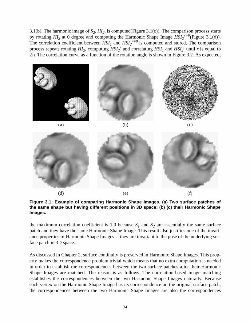
34

3.1(b). The harmonic image ofS2, HI2, is computed(Figure 3.1(c)). The comparison process startsby rotatingHI2 at 0 degree and computing the Harmonic Shape ImageHSI2

r=0(Figure 3.1(d)).The correlation coefficient betweenHSI1 andHSI2

r=0 is computed and stored. The comparisonprocess repeats rotatingHI2, computingHSI2

r and correlatingHSI1 andHSI2r until r is equal to

2π. The correlation curve as a function of the rotation angle is shown in Figure 3.2. As expected,

the maximum correlation coefficient is 1.0 becauseS1 and S2 are essentially the same surfacepatch and they have the same Harmonic Shape Image. This result also justifies one of the invari-ance properties of Harmonic Shape Images -- they are invariant to the pose of the underlying sur-face patch in 3D space.

As discussed in Chapter 2, surface continuity is preserved in Harmonic Shape Images. This prop-erty makes the correspondence problem trivial which means that no extra computation is neededin order to establish the correspondences between the two surface patches after their HarmonicShape Images are matched. The reason is as follows. The correlation-based image matchingestablishes the correspondences between the two Harmonic Shape Images naturally. Becauseeach vertex on the Harmonic Shape Image has its correspondence on the original surface patch,the correspondences between the two Harmonic Shape Images are also the correspondences

Figure 3.1: Example of comparing Harmonic Shape Images. (a) Two surface patches ofthe same shape but having different positions in 3D space; (b) (c) their Harmonic ShapeImages.

(a) (b) (c)

(d) (e) (f)

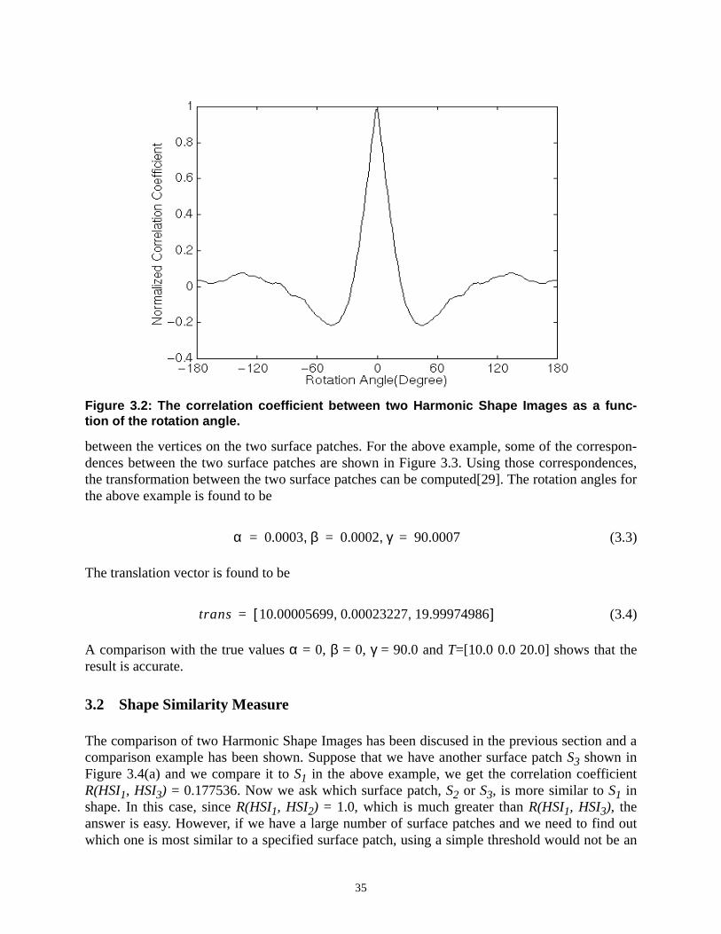
35

between the vertices on the two surface patches. For the above example, some of the correspon-dences between the two surface patches are shown in Figure 3.3. Using those correspondences,the transformation between the two surface patches can be computed[29]. The rotation angles forthe above example is found to be

(3.3)

The translation vector is found to be

(3.4)

A comparison with the true valuesα = 0, β = 0, γ = 90.0 andT=[10.0 0.0 20.0] shows that theresult is accurate.

3.2 Shape Similarity Measure

The comparison of two Harmonic Shape Images has been discused in the previous section and acomparison example has been shown. Suppose that we have another surface patchS3 shown inFigure 3.4(a) and we compare it toS1 in the above example, we get the correlation coefficientR(HSI1, HSI3) = 0.177536. Now we ask which surface patch,S2 or S3, is more similar toS1 inshape. In this case, sinceR(HSI1, HSI2) = 1.0, which is much greater thanR(HSI1, HSI3), theanswer is easy. However, if we have a large number of surface patches and we need to find outwhich one is most similar to a specified surface patch, using a simple threshold would not be an

Figure 3.2: The correlation coefficient between two Harmonic Shape Images as a func-tion of the rotation angle.

α 0.0003 β, 0.0002 γ, 90.0007= = =

trans 10.00005699 0.00023227 19.99974986, ,[ ]=

36

adequate answer. In this case, we would need a more sophisticated measurement in order to deter-mine how similar the most promising surface patch is to the specified patch. This measurement iscalled shape similarity measure. It is defined using the normalized correlation coefficientRbetween two Harmonic Shape Images as follows[44]:

(3.5)

The above shape similarity measure is a heuristic loss function that will return a high value fortwo highly correlated Harmonic Shape Images. The change of variables, a standard statisticaltechnique[22] performed by the hyperbolic arctangent function on the right hand side of (3.5),transforms the correlation coefficient into a distribution that has better statistical properties,namely, the variance of the distribution is independent ofR. In this case, the variance of the trans-formed correlation coefficient becomes1/(N-3), in which N is the number of correspondences inthe two Harmonic Shape Images[22].

Figure 3.3: Correspondences between the resampled meshes.

Figure 3.4: An example surface patch. (a) Rendered version; (b) wireframe version; (c) har-monic image; (d) Harmonic Shape Image.

(a) (b) (c) (d)

C S1 S2,( )1 R HSI1 HSI2,( )+

1 R HSI1 HSI2,( )–----------------------------------------------ln

=

37

Figure 3.5: Library of surface patches.

38

In order to explain how to use the shape similarity measure to determine a good matchbetween two surface patches, the following experiment is performed. Sixteen surface patchesare created from real objects and stored in a library (Figure 3.5). The patches are numbered from1 to 16 from top to bottom and from left to right in Figure 3.5. The first one is selected to be thetarget patch, and all the sixteen patches are compared with it by comparing their Harmonic ShapeImages to that of the first patch. The values of shape similarity measure are listed in Table 3.1.The histogram of those values are shown in Figure 3.6

Figure 3.6 shows that the shape similarity measure of the first patch to itself is much greater thanthat of the other patches. Obviously, it is the best match. However, this does not tell us how goodthis match is or how well it is distinguished from the other matches. Therefore, instead of using asimple threshold, a statistical method[22] is used to automatically detect the best match and deter-mine how good that match is. According to this method, good matches correspond to the outliersof a given histogram. The outliers are defined as follows. Suppose there areN values in the histo-gram. At the first step, the values are sorted and arranged from the lowest to the highest. At thesecond step, the median of the largestN/2 values is found and recorded as the upper fourth. Themedian of the smallestN/2 values is found and recorded as the lower fourth. At the third step, thefourth spread,fs, is computed as the difference between the upper fourth and the lower fourth. Atthe fourth step, the values that are greater than1.5fs from the upper fourth are determined to bemoderate outliers and the values that are greater than3fs from the upper fourth are determined tobe extreme outliers. In Figure 3.6, the cut-off value for extreme outliers is indicated by the linesegment. Because the shape similarity value of patch one to itself is above that cut-off, it is con-sidered to be well distinguished from other values. This means that the shape of surface patch oneis well distinguished from the shape of any other patch in the library.

Table 3.1: Shape Similarity Measure

1 2 3 4

3.8002 0.2142 0.1463 0.1223

5 6 7 8

0.1515 0.1899 0.2062 0.1629

9 10 11 12

0.3252 0.2045 0.1873 0.2320

13 14 15 16

0.1199 0.3033 0.1592 0.1893

39

3.3 Matching Surfaces by Matching Harmonic Shape Images

In the previous sections, we discussed how to match Harmonic Shape Images, how to defineshape similarity measure and how to automatically determine a good match based on the his-togram of the shape similarity measures. Remember that Harmonic Shape Images are onlypartial representations of given surfaces because they are based on surface patches; matchingHarmonic Shape Images is only an intermediate step in matching surfaces. In this section, wewill discuss how to match two surfaces by matching Harmonic Shape Images.

Given two surfaces, the matching process is illustrated in Figure 3.7. At the first step, a surfacepatchD2(v, R)on surfaceS2 is randomly selected and its Harmonic Shape ImageHSI(D2) is com-puted. At the second step, surface patches are created onS1 using some randomly selected verti-ces as centers and the specified radiusR. The Harmonic Shape Images of those surface patchesare computed and stored in a stack. At the third step, a search is conducted by matchingHSI(D2)to every Harmonic Shape Image in the stack ofS1. If a match is found, then at step four, the corre-

Figure 3.6: Histogram of the shape similarity measure.

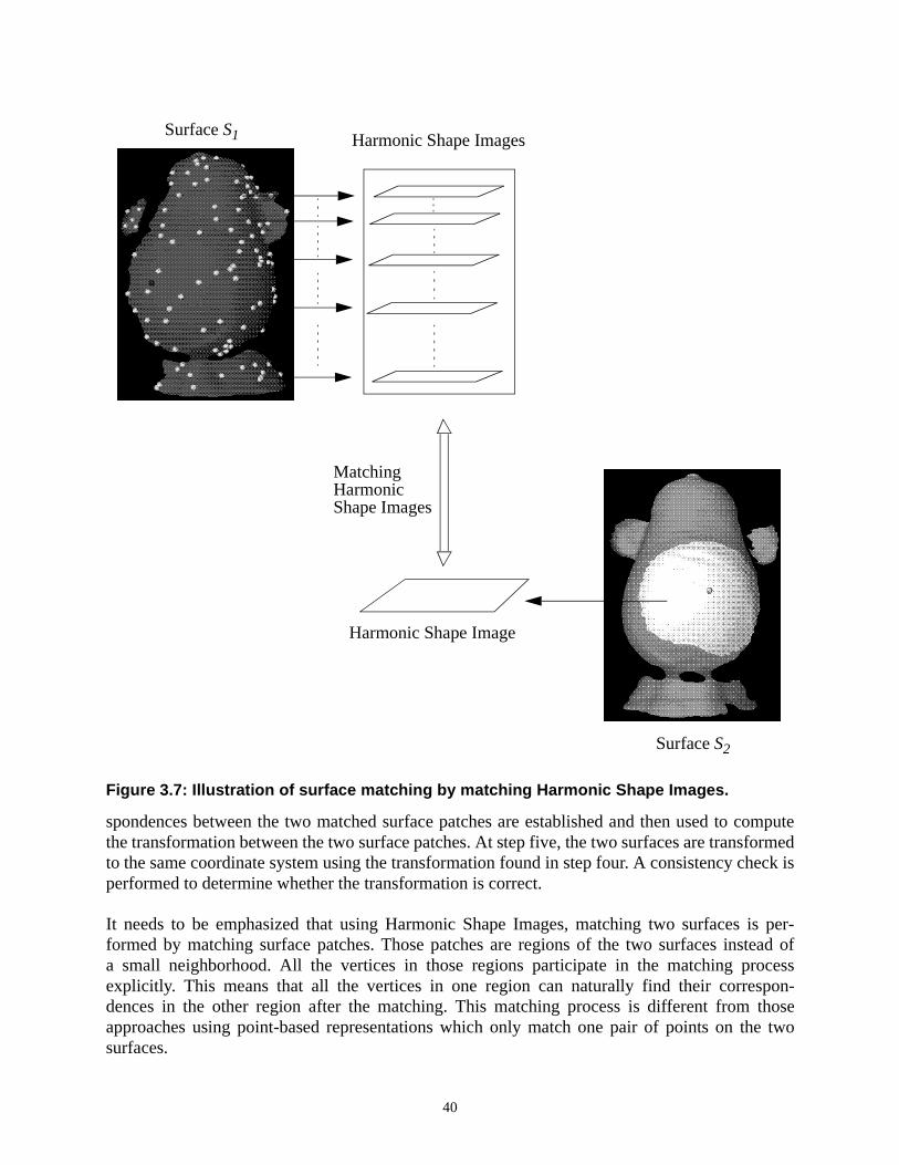
40

spondences between the two matched surface patches are established and then used to computethe transformation between the two surface patches. At step five, the two surfaces are transformedto the same coordinate system using the transformation found in step four. A consistency check isperformed to determine whether the transformation is correct.

It needs to be emphasized that using Harmonic Shape Images, matching two surfaces is per-formed by matching surface patches. Those patches are regions of the two surfaces instead ofa small neighborhood. All the vertices in those regions participate in the matching processexplicitly. This means that all the vertices in one region can naturally find their correspon-dences in the other region after the matching. This matching process is different from thoseapproaches using point-based representations which only match one pair of points on the twosurfaces.

Figure 3.7: Illustration of surface matching by matching Harmonic Shape Images.

SurfaceS1 Harmonic Shape Images

SurfaceS2

Harmonic Shape Image

MatchingHarmonicShape Images

41

Two issues that need to be discussed about the above surface matching strategy are choosingthe radius of surface patches and using a hierarchical approach to speed up the matching pro-cess.

Choosing the Radius of Surface Patches

The two main applications of surface matching are surface registration and object recognition.The strategies for choosing the radius of surface patches are different in the two cases. In thecase of surface registration, in general, there are two surfaces,S1 and S2, to be registered atone time.S1 and S2 partially overlap. The area ofS1 is denoted asA1 and the area ofS2 isdenotedA2. Assume . It is assumed that the area of the overlapping part is at least40% of theA1. The area of the surface patches used for matching is at least 25% ofA1. If a 2Ddisc model is used to approximate the surface patches, then the radius can be estimated by

.

In the case of object recognition, model surface patches are pre-created and stored in themodel library. During run-time, scene surface patches are created and compared with themodel surface patches. Because all the models are known before recognition and the scenesurfaces are partial surfaces of the models, the optimal radius of patches for matching may bedetermined before recognition.

Given an object surface as a model, some observations can be made for choosing the radius ofsurface patches on the model. If the radius is too small, then the surface patch will be smalland it will not have enough features to distinguish it from other patches on the model. In otherwords, if a small surface patch with few features is selected, then there may be so many qual-ified matches on the model that it is impossible to decide which one is the best match accord-ing to the statistical method we have discussed in the previous section. On the other hand, ifthe radius is too large, then there may be no matched patches at all on the model other than thepatch itself. This is not good for recognition because the sampling on the scene surfaces is notthe same as that on the model surfaces. As a result, there will not be any matched patches onthe scene surfaces. The following example illustrates how to choose the appropriate radius forsurface patches on a model surface.

Figure 3.8 shows an object with closed surface. Here, a closed surface is a triangular mesh inwhich every edge is associated with two triangles. A vertex,vc, is selected as the central vertex togenerate a series of target surface patches,Dt

i(vc, Ri), i=1...6. The radius,Ri, of this surface grad-ually increases so that the area of the corresponding surface patch increases from 5% to 30% ofthe entire area of the closed surface. Table 3.2 lists the radius with respect to each area percentage.

For each radiusRi, a library of model surface patches is created according to the following: Everyvertexvj, j= 1...n, is selected as the central vertex and a surface patch with radiusRi, Dm

i(vj, Ri), iscreated. Then the target model patch,Dt

i(vc, Ri), is compared with each patch in the model library

Table 3.2: Radius of Target Surface Patch with Respect to Area Percentage

Area Percentage 5% 10% 15% 20% 25% 30%

Radius 2.5 3.8 4.8 5.8 7.0 8.0

A1 A2≤

R 0.25A1 π⁄=

42

by comparing their Harmonic Shape Images. The shape similarity measure is computed for eachpair comparison and the histogram of all the shape similarity values is drawn. The statistic methodthat has been discussed in Section 3.2 is then used to find the qualified matches of the target sur-face patch among the model patches in the library. In the following, we present the comparisonresult for each radiusRi.

Figure 3.9(a) and (b) show the target surface patchDt1(vc, R1) with R1=2.5. Figure 3.9(c) shows

its Harmonic Shape Image. The histogram of the shape similarity values for the pairwise patchcomparison is shown in Figure 3.9(d). Here, it should be mentioned that a perfect match isobtained when the target patchDt

1(vc, R1) is compared to the model patchDm1(vc, R1) because the

two patches are the same. The similarity value for this comparison is not defined according to(3.5). Therefore, the histogram in Figure 3.9(d) does not include this value. This is the case for theremaining histograms which will be presented later in this section.

The vertical line segment in Figure 3.9(d) indicates the cut-off value for the qualified matches.There are no qualified matches in this case because the target surface patch does not have enoughfeatures to distinguish itself from the model surface patches in the library. In fact, the shape simi-larity values of the top 50 matches in the library are not high enough to qualify for the automaticselection of the statistical method. Figure 3.9(e) and (f) show the central vertices of those 50 topmatches. It can seen that the central vertices are at different locations of the model surface insteadof concentrating at the central vertex,vc, of the target surface patch. This result shows that thematching of the target surface patch is not successful.

Figure 3.8: An object with closed surface. (a) Rendered version; (b) Wireframe version.

(a) (b)

43

Figure 3.9: Target surface patch with radius Ri = 2.5. (a) Rendered version; (b) wireframeversion; (c) Harmonic Shape Image; (d) the histogram of the shape similarity values for thepairwise patch comparison between the target surface patch and the model patches; (e),(f) central vertices of the top 50 model matches in the library.

(a) (b)

(d)

(c)

(e) (f)

44

Now let us look at the case in whichR2 = 3.8. Figure 3.10(a), (b) and (c) show the target surfacepatchDt

2(vc, R2) and its Harmonic Shape Image, respectively. After comparing the target surfacepatch to the model patches in the library, the resultant histogram of the shape similarity values isshown in Figure 3.10(d). It can be seen that quite a few qualified matches are identified. In fact,the number of qualified matches is 50. Figure 3.10(e) shows the central vertices of those 50 sur-face patches. They are all around the central vertex,vc, of the target surface patch. This fact showsthat the target surface patch has been well identified among the model patches in the library.

Compared with previous case in whichRi = 2.5, the target surface patch withRi = 3.8 hasmore features that can be seen from its Harmonic Shape Image. This definitely helps identifysimilar model patches in the library. However, considering the number 50, there seem to betoo many qualified matches. In the following, we will continue increasing the radius of thetarget surface patch to determine whether the number of qualified matches decreases. Thiswill demonstrate how the radius of surface patches affects the matching result.

Figure 3.11(a), (b) and (c) show the target surface patchDt3(vc, R3) with R3 = 4.8 and its Har-

monic Shape Image. The histogram of matching results is shown in Figure 3.11(d). The centralvertices of the qualified patches are shown in Figure 3.11(e). In this case, the number of qualifiedmodel matches is still 50 and the central vertices of those surface patches are around the centralvertex,vc, of the target surface patch as well. Therefore, increasing the radius from 3.8 to 4.8 doesnot help to better identify the best matches in the model library because no new features are addedto the target surface patch with this increase.

In the cases in whichR4 = 5.8, R5 = 7.0 and R6 = 8.0, the corresponding target surfacepatches, their Harmonic Shape Images and the histograms of the pairwise patch comparisonresults are shown in Figure 3.12. The numbers of qualified matches in those three cases are 41, 18and 3, respectively. Therefore, increasing the radius of the target surface patch does help identifyit from the model patch library. However, it may not be realistic to use surface patches with largeradii in the application of object recognition because the full surface patches may not be seenfrom restricted viewing angles even without being occluded by other objects in the scene. Forexample, if the viewing direction is as shown in Figure 3.12(a1), (b1) and (c1), then the target sur-face patches with radii greater than 4.8 will be seen only partially. In fact, the resultant patcheswill have too much occlusion to be usable in recognition.

From the above example and discussion, it can be seen that the best value of the radius inorder to maintain both discrimination and stability is 4.8. In practice, a general guideline canbe made about selecting the radius of a surface patch in the application of object recognition.The lower bound of the radius of a surface patch can be determined by conducting the aboveexperiments. The upper bound can be determined using the viewing directions.

Hierarchical Matching Strategy

A hierarchical strategy can be used to speed up the matching process. Earlier in this section,we discussed a direct search approach to finding the best match on the second surface whengiven a surface patch on the first surface. Due to the stability of Harmonic Shape Images (thiswill be discussed in detail in the next chapter) meaning that neighboring vertices have similarsurface patches, the search can be conducted among part of the vertices on the second patch.

45

Figure 3.10: The target surface patch with Ri = 3.8. (a) Rendered version; (b) wireframe ver-sion; (c) Harmonic Shape Image; (d) histogram for the matching results; (e) the central ver-tices of the matched surface patches.

(a) (b) (c)

(d)

(e)

46

Figure 3.11: The target surface patch with Ri = 4.8. (a) Rendered version; (b) wireframe ver-sion; (c) Harmonic Shape Image; (d) histogram for the matching results; (e) the central ver-tices of the matched surface patches.

(a) (b) (c)

(d)

(e)

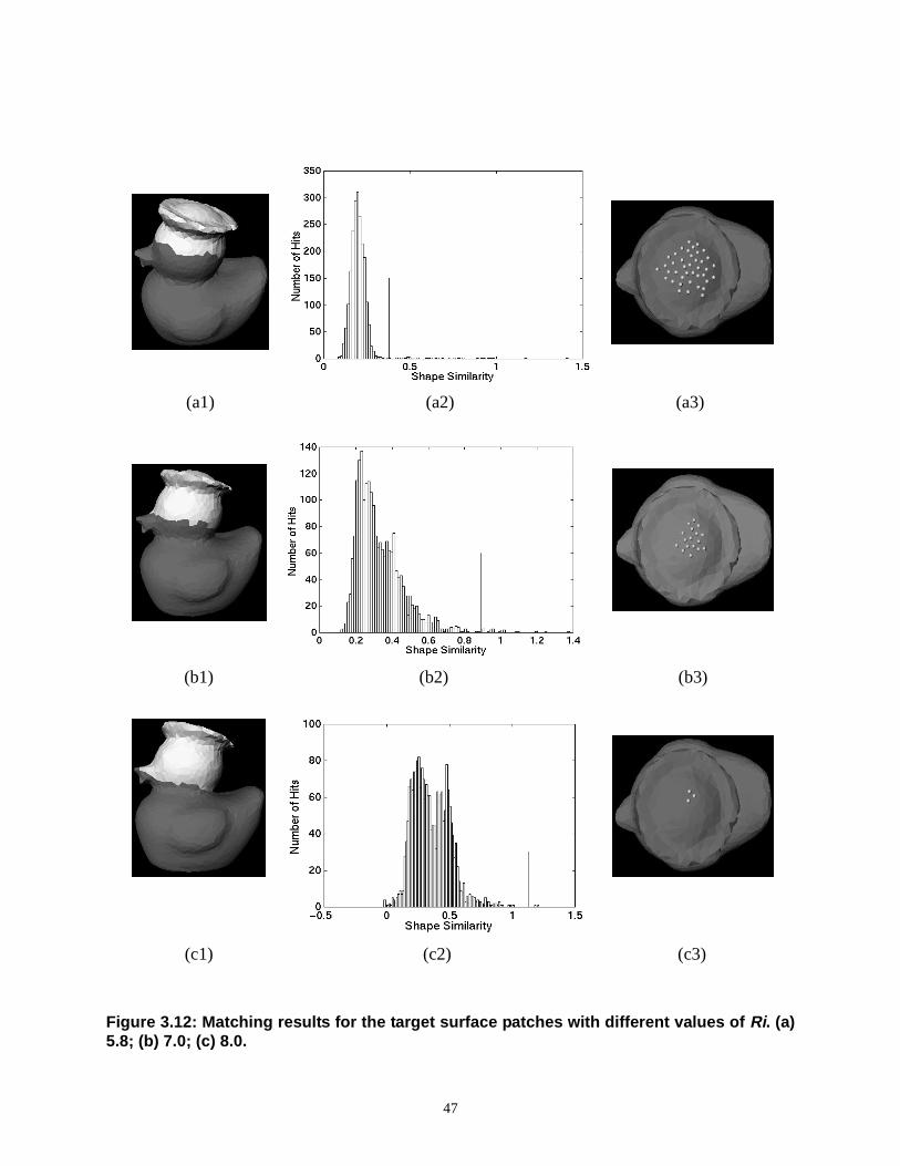
47

Figure 3.12: Matching results for the target surface patches with different values of Ri. (a)5.8; (b) 7.0; (c) 8.0.

(b2)

(a1)

(c1) (c2)

(b1)

(a2) (a3)

(b3)

(c3)

48

This is referred to as the coarse-level search. When the best match is found at the coarse level,it is further refined in the neighborhood of the best match at a finer resolution. This process isrepeated until the best match is found on the second surface. The hierarchical approach isillustrated using the following example.

Figure 3.13(a) and (c) show two surfacesS1 and S2 to be registered. The target surface patchDt

S1(v, R)is overlaid onS1 and shown in Figure 3.13(b) with its central vertexv highlightened. Inorder to apply the hierarchical search strategy,m vertices are randomly selected onS2 as centralvertices to generatem surface patches that will be compared with the target patchDt

S1(v, R). Inthis case,m = 100. The way to randomly select the central vertices is to use the pseudo randomnumber generator to generatem integers that are in the range of [0,n(S2)] with n being the numberof vertices onS2. Thosem central vertices are displayed in Figure 3.13(d). Ideally, them verticeswill distribute uniformly onS2 so that they construct a coarse resampling ofS2. It can be seenfrom Figure 3.13(d) that they are not distributed uniformly as expected. The reason for this is thatthe indices of the vertices are not necessarily related to their positions in the 3D space.

Figure 3.13: Illustration of the coarse-to-fine surface matching strategy.

(a) (b) (c) (d)

(e) (f) (g) (h)

49

In order to overcome the above resampling problem, a control strategy should be used whenselecting the central vertices so that they distribute as uniformly as possible on the surface.Before explaining how the control strategy works, let us define thenth-step neighbor of a ver-tex v on a triangular mesh.

• The1st-step neighbors ofv, , are the vertices that are connected tov by edges

• The 2nd-step neighbors of v, , are the vertices that satisfy

• The nth-step neighbors of v, , are the vertices that satisfy

The nth-step neighbors ofv can be interpreted as thenth-layer of vertices that are aroundv.The control strategy works as follows. At the first step, the first vertex is selected randomly.Then at the second step, a user-specified separation distanced, defined by the order ofnth-step neighbors, is used to determine which vertices are selected next. The rule is that theneighboring vertices ofv lower than the order ofd are not selected. And the neighboring ver-tices ofv with orderd are selected. At the third step, with each of the newly selected vertices,repeat the second step. The process stops when there are no more vertices to be selected. Thepseudo code for implementing the control strategy is the following.

// SelectedVerts: the array that stores the selected vertices// ToBeAddedVerts: the array that stores the vertices to be// added to SelectedVerts// Processed: a vertex is either labelled unselected or selected// or in ToBeAddedVertsvoid SelectSamplingVers(int StartVert, int SeparationDistance,IntArray SelectedVerts)

ToBeAddedVerts.push_back(StartVert);while ( ToBeAddedVerts is not empty )

CurrentVert = pop_front(ToBeAddedVerts);SelectedVerts.push_back(CurrentVert);GetNeighborsOfOrderD(CurrentVert, d, ToBeAdded);

void GetNeighborsOfOrderD(int CurrentVert, int SeparationDis-tance, IntArray ToBeAdded)

IntArray Queue;int i, i1, i2, i3;

i1 = 0; // head pointer to the current layeri2 = 1; // tail pointer to the current layeri3 = 1; // moving pointer for adding new vertices

Queue.push_back(CurrentVert);

u S1 v( )∈

w S2 v( )∈

w S1 u( ) u S1 v( ) w S1 v( )∉∧∈,∈

w Sn v( )∈

w S1 u( ) u Sn 1– v( ) w Sn 1– v( )∉∧∈,∈

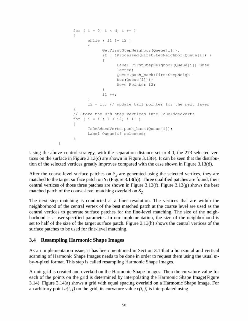
50

for ( i = 0; i < d; i ++ )

while ( i1 != i2 )

GetFirstStepNeighbor(Queue[i1]);if ( !Processed(FirstStepNeighbor(Queue[i]) )

Label FirstStepNeighbor(Queue[i]) unse-lected;Queue.push_back(FirstStepNeigh-bor(Queue[i]));Move Pointer i3;

i1 ++;

i2 = i3; // update tail pointer for the next layer

// Store the dth -step vertices into ToBeAddedVertsfor ( i = i1; i < i2; i ++ )

ToBeAddedVerts.push_back(Queue[i]);Label Queue[i] selected;

Using the above control strategy, with the separation distance set to 4.0, the 273 selected ver-tices on the surface in Figure 3.13(c) are shown in Figure 3.13(e). It can be seen that the distribu-tion of the selected vertices greatly improves compared with the case shown in Figure 3.13(d).

After the coarse-level surface patches onS2 are generated using the selected vertices, they arematched to the target surface patch onS1 (Figure 3.13(b)). Three qualified patches are found; theircentral vertices of those three patches are shown in Figure 3.13(f). Figure 3.13(g) shows the bestmatched patch of the coarse-level matching overlaid onS2.

The next step matching is conducted at a finer resolution. The vertices that are within theneighborhood of the central vertex of the best matched patch at the coarse level are used as thecentral vertices to generate surface patches for the fine-level matching. The size of the neigh-borhood is a user-specified parameter. In our implementation, the size of the neighborhood isset to half of the size of the target surface patch. Figure 3.13(h) shows the central vertices of thesurface patches to be used for fine-level matching.

3.4 Resampling Harmonic Shape Images

As an implementation issue, it has been mentioned in Section 3.1 that a horizontal and verticalscanning of Harmonic Shape Images needs to be done in order to request them using the usualm-by-n-pixel format. This step is called resampling Harmonic Shape Images.

A unit grid is created and overlaid on the Harmonic Shape Images. Then the curvature value foreach of the points on the grid is determined by interpolating the Harmonic Shape Image(Figure3.14). Figure 3.14(a) shows a grid with equal spacing overlaid on a Harmonic Shape Image. Foran arbitrary pointu(i, j) on the grid, its curvature valuec(i, j) is interpolated using

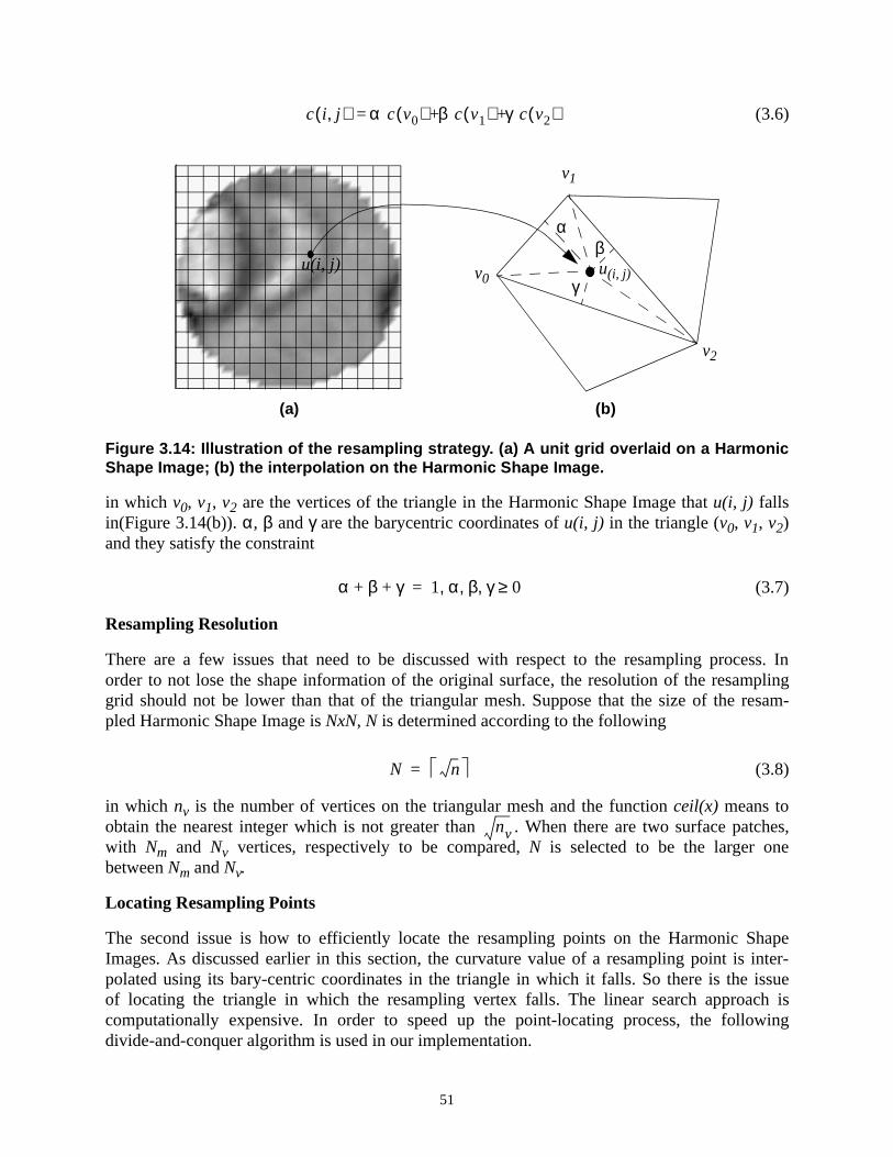
51

(3.6)

in which v0, v1, v2 are the vertices of the triangle in the Harmonic Shape Image thatu(i, j) fallsin(Figure 3.14(b)).α, β andγ are the barycentric coordinates ofu(i, j) in the triangle (v0, v1, v2)and they satisfy the constraint

(3.7)

Resampling Resolution

There are a few issues that need to be discussed with respect to the resampling process. Inorder to not lose the shape information of the original surface, the resolution of the resamplinggrid should not be lower than that of the triangular mesh. Suppose that the size of the resam-pled Harmonic Shape Image isNxN, N is determined according to the following

(3.8)

in which nv is the number of vertices on the triangular mesh and the functionceil(x) means toobtain the nearest integer which is not greater than . When there are two surface patches,with Nm and Nv vertices, respectively to be compared,N is selected to be the larger onebetweenNm andNv.

Locating Resampling Points

The second issue is how to efficiently locate the resampling points on the Harmonic ShapeImages. As discussed earlier in this section, the curvature value of a resampling point is inter-polated using its bary-centric coordinates in the triangle in which it falls. So there is the issueof locating the triangle in which the resampling vertex falls. The linear search approach iscomputationally expensive. In order to speed up the point-locating process, the followingdivide-and-conquer algorithm is used in our implementation.

Figure 3.14: Illustration of the resampling strategy. (a) A unit grid overlaid on a HarmonicShape Image; (b) the interpolation on the Harmonic Shape Image.

c i j,( ) αc v0( ) βc v1( ) γc v2( )+ +=

v1

v0

v2

u(i, j)

βα

γu(i, j)

(a) (b)

α β γ+ + 1 α β γ 0≥, , ,=

N n=

nv

52

The unit grid is first divided intomxmbins.m is selected as

(3.9)

in which nt is the number of triangles in the Harmonic Shape Image andT is a constant thatadjusts the number of bins. In our implementation,T is set to 10. After the bins are set up, thetriangles are stored into those bins. This is done by first storing the vertices into correspondingbins. At the next step, for each triangleTi = (vj, vk, vl), the bin indices for each of its verticesare denoted as as shown in Figure 3.15. Then the minimum and

maximum of bin indices of the three vertices are found forbinx and biny and are denoted asmin(binx), max(binx), min(biny), max(biny). Then the bins that the triangleTi is in can be deter-mined as . This means that inFigure 3.15, all the bins are considered as containing the triangleTi. Obviously, this strategy isconservative in that it takes into account some bins that do not containTi, e.g., the bins in Figure3.15 labelled with question marks. Because it takes much more effort to determine the exact thenumber of bins that the triangle is in, the cost of taking extra bins into account is ignored.

After all the triangles are stored into the bins, each resampling vertex will be located in a spe-cific triangle using this information. First of all, it is easy to locate the bin that the resamplingvertex falls in using its coordinates. Second, since there may be a number of triangles in thatbin, a linear search is needed to locate the right triangle. The criterion for locating the right tri-angle is to compute the bary-centric coordinates for the resampling vertex in each triangle in

Figure 3.15: Locating resampling points using the divide and conquer strategy.

mnt

T--------=

bin vj( ) binx vj( ) biny vj( ),( )=

vl

vk

vj

(min(binx), max(biny)) (max(binx), max(biny))

(min(binx), min(biny)) (max(binx), min(biny))

? ?

?

?

? ? ?

bin i j,( ) min binx( ) i max binx( ) min biny( ) j max biny( )≤ ≤,≤ ≤

53

that bin. If the bary-centric coordinates satisfy (3.7), then the resampling vertex falls into that tri-angle. The bary-centric coordinates can be obtained by solving the following equations. Let (xi,yi), i=0, 1, 2 denote the coordinates of verticesvi, i=0, 1, 2, on the Harmonic Shape Image. Let (x,y) denote the coordinates of the resampling pointu. Then the following equations hold

(3.10)

(3.10) can be written in matrix form as (3.11)

(3.11)

The unknown vector [α, β, γ]T can be solved as follows:

(3.12)

According to the way the interior mapping is constructed, there should not be any degeneratedtriangles. This means that the matrix in (3.12) always has full rank. In our implementation, rankchecking is still performed in case of any numerical problems caused by skinny triangles.

Invalid Resampling Points

Because a unit grid is overlaid on the Harmonic Shape Image which is defined on a unit disc,some resampling points are outside that image(Figure 3.14(a)). Those resampling points arelabelled invalid so that they do not participate in the correlation-based image matching. Invalidresampling points can be caused by occlusion as well. In this case, those invalid resampling pointsare inside the unit circle. Their curvature values are labeled invalid on the Harmonic ShapeImage.

Validity of the Resampling Grid

The resampling grid shown in Figure 3.14(a) has equal spacing among all points. This kind of res-ampling scheme is called parametric uniform resampling. No matter what resampling scheme isused, its goal is to resample the original surface patches as uniformly as possible so that they canbe compared in a meaningful way. For example, there are three surface patches shown in Figure3.16(a1), (b1), (c1). Their harmonic images are shown in (a2), (b2) and (c2), respectively. The

αx0 βx1 γx2+ + x=

αy0 βy1 γy2+ + y=

α β γ+ + 1=

x0 x1 x2

y0 y1 y2

1 1 1

αβγ

x

y

1

=

αβγ

x0 x1 x2

y0 y1 y2

1 1 1

1–x

y

1

=

54

resampled meshes for those three surfaces shown in (a3), (b3) and (c3) are obtained by using thesame interpolation strategy that has been used to generate Harmonic Shape Images. The only dif-ference is that, instead of interpolating the curvature distribution function on the harmonic image,the coordinate function is interpolated.

Figure 3.16: Examples of surface patches and their resampled versions. (a1), (b1, (c1)Three surface patches in wireframe; (a2), (b2), (c2) their harmonic images; (a3), (b3), (c3)the resampled meshes; (a4), (b4), (c4) their Harmonic Shape Images.

(a1) (a2) (a3) (a4)

(b1) (b2) (b3) (b4)

(c1) (c2) (c3) (c4)

55

As can be seen In Figure 3.16(a3), (b3), the reconstructed meshes are reasonably uniform. How-ever, in Figure 3.16(b3), there is significant difference between the densities of resampling pointson different parts of the reconstructed surface. In this case, the Harmonic Shape Image in Figure3.16(b4) is not a good representation of the original surface. Therefore, comparing the surfacepatches in Figure 3.16(a1) and (c1) by comparing their Harmonic Shape Images in Figure3.16(a4) and (c4) is not meaningful because Figure 3.16(c4) does not represent the shape of Fig-ure 3.16(c1) correctly.

The above discussion suggests that, before conducting resampling, it is necessary to checkwhether the uniform resampling grid is appropriate for the underlying harmonic image. In thefollowing, we will first discuss why it is not appropriate for some Harmonic Shape Imagesand then we will present a method to check its validity.

Recall that resampling is performed on the harmonic image of a given surface patch. If theuniform resampling strategy is used, then the resampling result depends solely on the distribu-tion of vertices on the harmonic image. Let us look at the harmonic images in Figure 3.16 as anexample. The distribution of vertices in the harmonic images shown in Figure 3.16(a2) and (b2) isreasonably uniform. Therefore, the two resampled surfaces in Figure 3.16(a3) and (b3) are goodenough to represent the original surfaces in Figure 3.16(a1) and (b1). In contrast, there is a highconcentration of vertices in the harmonic image shown in Figure 3.16(c2). When uniform resam-pling is performed on it, the resampled mesh shown in (c3) is not a good reconstruction of theoriginal surface patch. The reason for this problem is that, although the high concentration of ver-tices takes up only a small area in the harmonic image, their correspondences in the original sur-face patch actually take up a much larger area of the entire surface. In other words, there is muchhigher area compression for those triangles than for others in the original surface when beingmapped onto the harmonic image. The area compression depends only on the shape of the under-lying surface patch. In general, the more a surface patch is curved, the more area compressionthere is on its harmonic shape image.

After determining that the area compression is intrinsic to the shape of the surface patch, wehave two approaches to solving the resampling problem. We perform a pre-processing step todetermine whether uniform resampling will generate good resampled meshes. At this step, a1D histogram called Area Histogram is created for each harmonic image and compared to apre-stored histogram. If the newly generated Area Histogram is not consistent with the pre-stored one, then it is determined to be abnormal and no resampling will be performed on thatharmonic image.

The area histogram is generated as follows. Given a unit disc and a certain number of concentriccircles on that disc(Figure 3.17(a)), if the mass density of the disc is uniform everywhere, then wecan compute the area (it is proportional to the mass) of each disc with increasing radius along theradial direction. The curve called the area histogram of the disc, which characterizes the relation-ship between radius and disc area, is denoted as a solid line in Figure 3.18. Now let us perform thesame computation on a harmonic image with two modifications(Figure 3.17(b)). The first is thatthe harmonic image is discrete. The area of each disc with different radius is computed as the sumof the area of the triangles in that disc. The second modification is that the area of each triangle inthe harmonic image is not its actual area. Rather, it is the ratio between the area of its correspon-

56

dence triangle in the original mesh and the entire area of the original mesh. If the degree of areacompression does not vary much across the harmonic image, then the area histogram of the har-monic image will be similar to that of the unit disc. Figure 3.18 shows the area histograms ofsome surface patches in Figure 3.16 and Figure 3.19.

Figure 3.17: Illustration of area histogram.

Figure 3.18: Area histograms of the surface patches in Figure 3.16 and Figure 3.19.

r r

(a) (b)

--: Discx: Figure3.16(a1)o: Figure3.16(b1)+: Figure3.19(a1)

: Figure3.19(b1): Figure3.16(c1): Figure3.19(d1)

*: Figure3.19(c1)

57

Figure 3.19: Examples of surface patches, their harmonic images, resampled patches, andHarmonic Shape Images.

(a1) (a2) (a3) (a4)

(b1) (b2) (b3) (b4)

(c1) (c2) (c3) (c4)

(d1) (d2) (d3) (d4)

58

Figure 3.18 shows that all the area histograms, except for the one for the surface patch in Figure3.16(c1), are consistent with the area histogram of the disc. And their resampled meshes are rea-sonably uniform. In our implementation, the area histogram of the disc is pre-stored as the stan-dard so that the area histograms of harmonic images can be compared with it. The result of thecomparison determines whether uniform resampling can be performed on those harmonic images.

It should be pointed out that the distribution of vertices on the original surface patch does notaffect the resampling strategy. Nor does it affect the area histogram. The surface patch in Figure3.19(d1) is an example of this. The patch has the same shape as the surface patch in Figure3.16(a1) but with different distribution of vertices. Its area histogram is very close to that of thesurface patch in Figure 3.16(a1) (Figure 3.18). Using the uniform resampling strategy, the distri-bution of vertices on the resampled mesh (Figure 3.19(d3) is comparable to that in Figure3.16(a3). As a summary, area histogram is a reliable way to detect whether uniform resampling isappropriate for resampling Harmonic Shape Images.

Area histogram can also be used to pre-eliminate unlikely matches from the search space becauseit is only determined by the shape of the underlying surface patch. In other words, the histogram isintrinsic to the shape of the surface patch. Therefore, if two surface patches have completely dif-ferent area histograms, e.g., the surface patches in Figure 3.16(a1) and (c1), then they have differ-ent shapes. This pre-elimination can save the time for correlating the Harmonic Shape Images ofthose two surface patches.

Area histogram is a more formal way to check the validity of the uniform resampling grid.Another quick checkup can be performed by computing the ratio between the area and the cir-cumference of the surface patch. When the ratio is high, it means that a large area is enclosed by asmall circumference. In this case, the area compression is usually high on its harmonic image.

59

Chapter 4

Experimental Analysis of Harmonic Shape Images

The concept of Harmonic Shape Images -- how to generate and match Harmonic ShapeImages, has been discussed in previous chapters. In this chapter, some properties of HarmonicShape Images under different sources of noise are investigated. Due to the fact that it is diffi-cult to obtain an analytical function of the Harmonic Shape Images with respect to noise suchas surface resolution and occlusion, an experimental approach is employed to demonstratingthe performances of the images.

In this chapter, four properties of Harmonic Shape Images are investigated: discriminability,stability, robustness to surface resolution and robustness to occlusion. In the following, thesefour properties are briefly introduced, followed by the introduction of the experimental setup.

Discriminability: Discriminability describes how discriminative a representation’s ability todiscern surfaces of different shapes. This is the basic requirement for all representations.

Stability: Stability measures the capability of representting surfaces of similar shapes usingsimilar representations. This means that the representation does not change significantly whenthere are small changes on the underlying surface. Stability is an important property whenconducting surface matching, e.g., it enables the use of the coarse-to-fine matching strategy.Detailed explanations are given in the following sections.

Robustness to surface resolution:In practice, the surfaces we deal with are discretek, i.e., notwo surfaces to be compared have exactly the same sampling resolution. Without the propertyof being robust to surface resolution, the representations for surfaces of the same shape but ofdifferent sampling will be different. Obviously this is not what we expected from a qualifiedrepresentation for surface matching.

Robustness to occlusion:Occlusion occurs quite often in practice either because of selfocclusion or occlusion by other objects. In its presence, we should still be able to conduct sur-face matching using the non-occluded parts of the surfaces. This requires that the representa-tion for the non-occluded parts of the surfaces remain approximately the same as that whenthere is no occlusion. Without the robustness to occlusion, surface matching would fail imme-diately when there is a small percentage of occlusion on the surfaces to be compared.

The basic setup of the experiments for testing the four properties are essentially the same. Inthe following, three key components of the setup are explained, including patch library,matching procedure and display format.

Patch Library: One or more libraries of surface patches are used in each experiment. Alto-gether there are three different kinds of libraries. The first consists of ten patches generated byusing different parametric functions. The second one consists of sixteen patches extractedfrom real objects of different shapes. The third one consists of patches generated from thesame real object. In some experiments, extensions are added to the second library by addingnew surface patches.

60

Matching Procedure: A Harmonic Shape Image for each surface patch in a library is com-puted and stored. Then every patch is compared with every other one by comparing their Har-monic Shape Images, and the shape similarity value is computed. Suppose there aren patchesin a library; there aren2 shape similarity values including self-comparison of every patch.

Display Format: There are two display formats for the comparision result in each experi-ment. The first is a three-dimensional height field with theX and Y axes representing the indi-ces of the surface patches in the library and theZ axis representing the shape similarity valuefor every pair of surface patches. For example, if there aren patches in the library, then therange of indices for theX andY axes is and , respectively. The shape sim-ilarity value for the patches (i, j) is represented byz(i, j). This display format is referred as theshape similarity matrix. The matrix is symmetric, i.e., because the shape sim-ilarity measure is symmetric. This display format provides an overall view of the comparisonresults among the surface patches in the library. The second display format is a histogram ofthe shape similartiy values for one patch as compared with all the patches in the library. Theintepretation of the histogram has been discussed in Chapter 3. This display format provides aninside look at how different a surface patch is when compared to others.

In the following sections, each of the four properties of Harmonic Shape Images will be ana-lyzed using the experimental approach that has been discussed above.

4.1 Discriminability

One of the important properties of shape representation is its ability to discriminate surfacesof different shapes. This is referred as the discriminability of a shape representation. In thissection, the discriminability of Harmonic Shape Images is investigated under two differentscenarios. In the first scenario, we study the discriminability of Harmonic Shape Imageswithin a collection of surface patches of different shapes. The aim is to check whether any twosurface patches can be distinguished according to their Harmonic Shape Images. In the secondscenario, we study the discriminability on the surface of an individual object. This scenario isquite common in the application of object recognition. The aim of this experiment is to checkwhether a surface patch on the object surface can be distinguished effectively from otherpatches on the object surface according to their Harmonic Shape Images.

Two libraries of surface patches are created for conducting the first experiment. One libraryconsists of 10 patches extracted from 10 different parametric surfaces. The 10 surfacespatches and their Harmonic Shape Images are shown in Figure 4.1. All the patches have the sameradius. Among those patches, every pair is compared by matching their Harmonic Shape Images.The comparison result is summarized in a matrix form as shown in Figure 4.2. Figure 4.2(a)shows the normalized correlation coefficient for the comparison of every pair of surface patches.TheX-axis andY-axis represent the indices of surface patches from 1 to 10. TheZ-axis representsthe normalized correlation coefficients, i.e.,z(i, j) is the correlation coefficient of surface patchesi and j. Figure 4.2(a) shows that, the correlation coefficients on the diagonal are all equal to 1.0,while the correlation coefficients elsewhere are much lower than that. This simply shows the factthat every surface patch is completely correlated to itself in shape but not so to other patches.

i 1 n,[ ]∈ j 1 n,[ ]∈

z i j,( ) z j i,( )=

61

Figure 4.1: The library of 10 surface patches extracted from 10 parametric surfaces.

(1) (2)

(3) (4)

(5) (6)

(7) (8)

(9) (10)

62

Figure 4.2: Pair comparison results of the surface patches in the first library. (a) The re-sultant matrix of the normalized correlation coefficients; (b) the resultant matrix of theshape similarity measure.

(a)

(b)

63

In order to quantify the difference between one surface patch and all the other patches, theshape similarity measure is computed for every pair comparison of surface patches. Figure 4.2(b)shows the resultant shape similarity matrix. The matrix in Figure 4.2(b) is similar to the matrix inFigure 4.2(a) and the shape difference between any patch and other patches is more obvious. Fig-ure 4.3 and Figure 4.4 show the histogram of every row or column of the shape similarity matrixin Figure 4.2(b). Each histogram shows how different a surface patch is compared to all thepatches in the library. The cut-off value for the qualified match is indicated by a line segment inevery histogram. It can been seen that every surface patch is the only qualified match to itself, andthat this match is well above the threshold of the qualified match.

The second library consists of 16 patches extracted from real objects. The patches and theirHarmonic Shape Images are shown in Figure 4.5 and Figure 4.6, respectively. The pair compari-son results are shown in Figure 4.7 , Figure 4.8, Figure 4.9 and Figure 4.10. This example thateach surface patch can be effectively discriminated from other patches in the library by using Har-monic Shape Images.

The next experiment is conducted among the surface patches extracted from the same object.The object is shown in Figure 4.11(a) with the target surface patch overlaid on it. The target patchhas radiusR = 2.0. Its wireframe and Harmonic Shape Images are shown in Figure 4.11(b) and(c), respectively. There are 2137 vertices on the object. Every vertex is used as the central vertexto generate a surface patch withR = 2.0. The matching is conducted between the target patch andeach of the 2137 patches. The histogram of the shape similarity values from the matching isshown in Figure 4.12. It can be seen that a number of surface patches are above the qualifiedmatch threshold. The central vertices of those patches are shown in Figure 4.11(d).

From the above result, it can be seen that the target patch can be distingushed from 99.16% ofthe total number of patches on that object. This shows that the Harmonic Shape Image of thetarget surface patch is discriminative enough. However, a question may be asked why the tar-get patch cannot be identified as uniquely as that in the previous two experiments. The answeris that the surface patches in the previous two libraries came from different objects and thosepatches are different from one another in shape. There is no relationship of any kind betweenany two patches. Therefore, a surface patch can always be identified uniquely. However, inthis example, all the surface patches come from the same smooth surface. There are surfacepatches of similar shape because the central vertices of those patches are neighboring verticesand all the surface patches have the same radius. Under such circumstances, a target patchshould only be matched to those patches that have similar shape. It should still be discrimi-nated from other patches that have different shapes. The results shown in Figure 4.11(d) and Fig-ure 4.12 demonstrate that the result is just as what we expected. The central vertices of thequalified patches are neighbors of the central vertex of the target patch. Figure 4.13 shows twoqualified patches and their Harmonic Shape Images.

4.2 Stability

Stability is another important property of Harmonic Shape Images. Unlike discriminabilitywhich measures the capability of discriminating different shapes, stability measures the capa-bility of identifying similar shapes. This property is extremely useful in the following two sce-narios. The first one is that the surfaces we are dealing with in practice are discrete; therefore,

64

Figure 4.3: Histogram of the shape similarity values for surface patch 1 through 6 toother patches.

(1) (4)

(2) (5)

(3) (6)

65

it is almost impossible to have two surface patches be exactly the same due to the differencesin sampling resolution. In this case, given a target patch on one surface, we cannot expect tofind its match on the second surface with exactly the same central vertex as that of the targetpatch. In fact, there may be patches on the second surface that have central vertices that arevery close to the central vertex of the target patch. Using Harmonic Shape Images, thosepatches should be identified correctly.

The second scenario is that, given one target patch on the first surface, we can sub-sample thesecond surface in order to speed up the matching process if we have the knowledge thatneighboring vertices on a surface have similar patches and Harmonic Shape Images. In fact,we have already seen the application of this property in Chapter 3, in which the coarse-to-finematching strategy was discussed. That strategy is based on the stability property of HarmonicShape Images.

Figure 4.4: Histogram of the shape similarity value for every surface patch 7 through 10to other patches.

(7) (9)

(8) (10)

66

Figure 4.5: The patches 1 through 8 and their Harmonic Shape Images in the secondlibrary.

(1) (2)

(3) (4)

(5) (6)

(7) (8)

67

Figure 4.6: The patches 9 through 16 and their Harmonic Shape Images in the secondlibrary.

(9) (10)

(11) (12)

(13) (14)

(15) (16)

68

Figure 4.7: Pair comparison results of the surface patches in the second library. (a) Theresultant matrix of the normalized correlation coefficients; (b) the resultant matrix of theshape similarity measure.

(a)

(b)

69

Figure 4.8: Histogram of the shape similarity values for surface patches 1 through 6 toother patches in the second library.

(1) (4)

(2) (5)

(3) (6)

70

Figure 4.9: Histogram of the shape similarity values for patches 7 through 12 to otherpatches in the second library.

(7) (10)

(8) (11)

(9) (12)

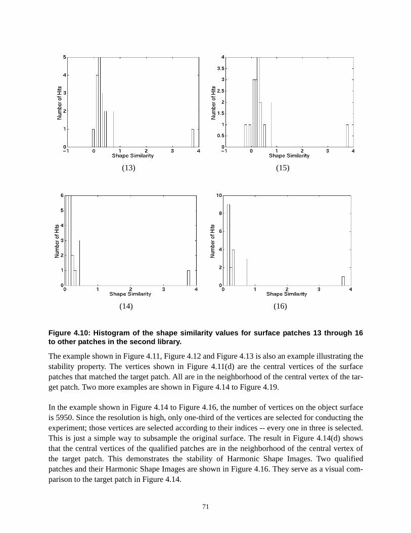
71

The example shown in Figure 4.11, Figure 4.12 and Figure 4.13 is also an example illustrating thestability property. The vertices shown in Figure 4.11(d) are the central vertices of the surfacepatches that matched the target patch. All are in the neighborhood of the central vertex of the tar-get patch. Two more examples are shown in Figure 4.14 to Figure 4.19.

In the example shown in Figure 4.14 to Figure 4.16, the number of vertices on the object surfaceis 5950. Since the resolution is high, only one-third of the vertices are selected for conducting theexperiment; those vertices are selected according to their indices -- every one in three is selected.This is just a simple way to subsample the original surface. The result in Figure 4.14(d) showsthat the central vertices of the qualified patches are in the neighborhood of the central vertex ofthe target patch. This demonstrates the stability of Harmonic Shape Images. Two qualifiedpatches and their Harmonic Shape Images are shown in Figure 4.16. They serve as a visual com-parison to the target patch in Figure 4.14.

Figure 4.10: Histogram of the shape similarity values for surface patches 13 through 16to other patches in the second library.

(13) (15)

(14) (16)

72

The example object surface shown in Figure 4.17 has 3684 vertices. Half of those vertices areselected for conducting the stability experiment. The central vertices of the qualified matches areshown in Figure 4.17(d). Figure 4.18 shows the histogram of the shape similarity values of thematching result. Figure 4.19 shows that the examples of the matched patches are quite similar tothe target patch in Figure 4.17.

4.3 Robustness to Resolution

It has been discussed in Chapter 2 that Harmonic Shape Images do not depend on any specificsampling strategy, e.g., uniform sampling. For a given surface, as long as the sampling rate is highenough such that the shape of the surface can be sufficiently represented, its Harmonic ShapeImage is also accurate enough for surface matching. It should be noted that the comparison of

Figure 4.11: Identify one surface patch from all the surface patches on one object. (a)The target surface patch overlaid on the object; (b) the wireframe version of the target sur-face patch; (c) the Harmonic Shape Image of the target surface patch; (d) the central verti-ces of the qualified surface patches that match the target patch.

(a) (b)

(c) (d)

73

Figure 4.12: Histogram of the shape similarity values from the matching experiment.

Figure 4.13: Examples of the qualified patches of the target patch in Figure 4.11.

(a) (b)

(c) (d)

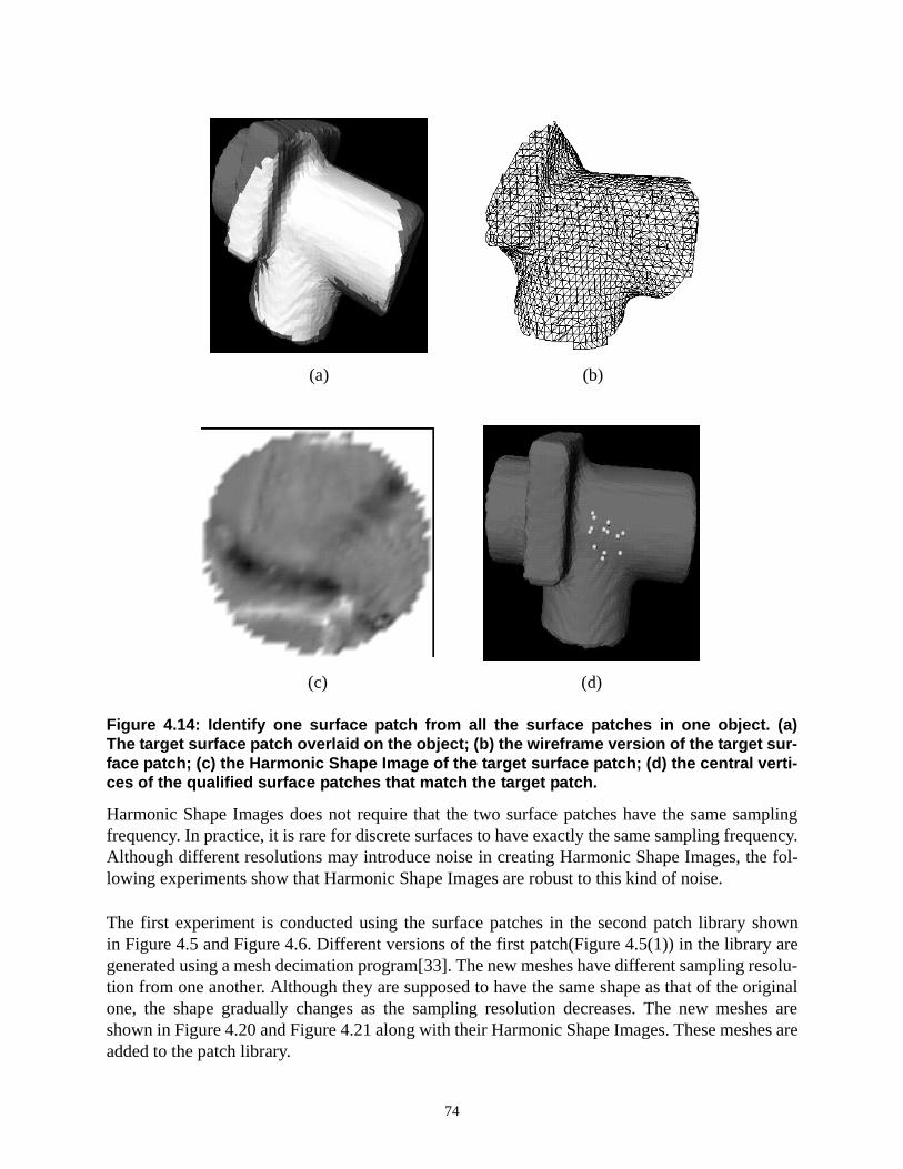
74

Harmonic Shape Images does not require that the two surface patches have the same samplingfrequency. In practice, it is rare for discrete surfaces to have exactly the same sampling frequency.Although different resolutions may introduce noise in creating Harmonic Shape Images, the fol-lowing experiments show that Harmonic Shape Images are robust to this kind of noise.

The first experiment is conducted using the surface patches in the second patch library shownin Figure 4.5 and Figure 4.6. Different versions of the first patch(Figure 4.5(1)) in the library aregenerated using a mesh decimation program[33]. The new meshes have different sampling resolu-tion from one another. Although they are supposed to have the same shape as that of the originalone, the shape gradually changes as the sampling resolution decreases. The new meshes areshown in Figure 4.20 and Figure 4.21 along with their Harmonic Shape Images. These meshes areadded to the patch library.

Figure 4.14: Identify one surface patch from all the surface patches in one object. (a)The target surface patch overlaid on the object; (b) the wireframe version of the target sur-face patch; (c) the Harmonic Shape Image of the target surface patch; (d) the central verti-ces of the qualified surface patches that match the target patch.

(a) (b)

(c) (d)

75

Figure 4.15: Histogram of the shape similarity values for the matching experiment in Figure4.14.

Figure 4.16: Examples of the qualified patches of the target patch in Figure 4.14(b).

(a) (b)

(c) (d)

76

As in the previous experiments, pair comparison is performed for every pair of surfacepatches in the extended library. The expected result is that the new patches are identified to besimilar to the original patch and different from other patches in the library. Figure 4.22(a) and (b)show the comparison result. The matrix of the normalized correlation coefficients is shown inFigure 4.22(a). As before, the correlation coefficients on the diagonal are self-comparison foreach patch in the library, therefore having the value of 1.0. In addition to the diagonal, there arehigh correlation values between the patches indexed from 17 to 23 to the first patch. The patchesindexed from 17 to 23 are the patches of the same shape as patch one but are of different resolu-tions. The correlation values for the pair comparison among those patches 17 to 23 are also highas shown in Figure 4.22(a) by the block in the back of the figure. This distribution of correlationvalues is exactly as we had expected. The matrix of shape similarity values in Figure 4.22(b) alsoverifies this result.

Figure 4.17: Identify one surface patch from all the surface patches in one object. (a)The target surface patch overlaid on the object; (b) the wireframe version of the target sur-face patch; (c) the Harmonic Shape Image of the target surface patch; (d) the central verti-ces of the qualified surface patches that match the target patch.

(a) (b)

(c) (d)

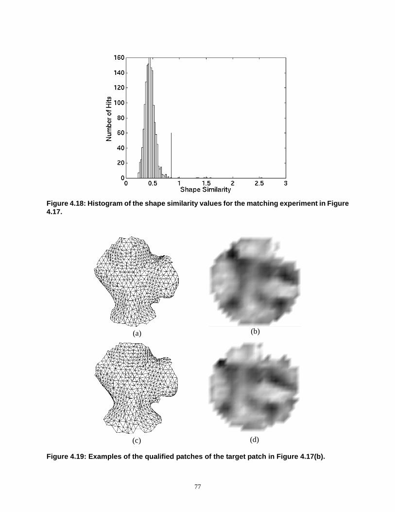
77

Figure 4.18: Histogram of the shape similarity values for the matching experiment in Figure4.17.

Figure 4.19: Examples of the qualified patches of the target patch in Figure 4.17(b).

(a) (b)

(c) (d)

78

Figure 4.20: Surface patches of the same shape but of different resolutions. Left col-umn: rendered surfaces; middle column: surfaces in wireframe; right column: Harmon-ic Shape Images: From top to bottom, the number of vertices are 2073, 1689, 1344 and1028.

79

Figure 4.21: Surface patches of the same shape but of different resolutions. Left col-umn: rendered surfaces; middle column: surfaces in wireframe; right column: Harmon-ic Shape Images: From top to bottom, the number of vertices are 686, 324, 169 and 82.

80

Figure 4.22: Pair comparison results of the surface patches in the second library afteradding the surface patches with different resolution. (a) The result matrix of normalizedcorrelation coefficients; (b) the result matrix of shape similarity measure.

(a)

(b)

81

In order to show clearly how similar the new patches are to the original patch and how differ-ent they are from other patches, histograms of the shape similarity values in Figure 4.22(b) areshown in Figure 4.23. There, the number of qualified matches is 79. This includes the self com-

parison(23), the new patches to the original patch and vice versa(7x2=14) and the pair comparisonamong the new patches(7x6=42). Figure 4.24 and Figure 4.25, show the histogram for every newpatch compared to the 16 patches in the library is shown. It can been seen that the new patches 1to 6 can be determined effectively to be similar to the first patch. However, as shown in Figure4.25(7), the shape similarity value between new patch 7 and patch 1 is a moderate outlier amongthe shape similarity values between new patch 7 to all the 16 patches. This shows that, althoughpatch 7 can still be determined to be similar to patch 1, the confidence level decreases when com-pared with the other 6 new patches. The reason for this is that the sampling resolution of newpatch 7 is very low compared to patch 1. Therefore, there is significant change in both the bound-ary and the shape of new patch 7. The curve of normalized correlation coefficients as a function ofthe sampling resolution is shown in Figure 4.26. Here, the sampling resolution is defined as theratio between the number of vertices on each of the new patches and the number of vertices onsurface patch 1. As the sampling resolution decreases, the normalized correlation coefficientdecreases gracefully. This demonstrates the robustness of Harmonic Shape Images with respect tosampling resolution.

The second experiment is conducted in the same way as was the first experiment. Seven newpatches of the same shape as that of patch 2 in the library, but of different sampling resolu-tions, are generated and added to the 16-patch library. The new patches and their HarmonicShape Images are shown in Figure 4.27 and Figure 4.28. The pair comparison results are shown inFigure 4.28, Figure 4.29, Figure 4.30, Figure 4.31 and Figure 4.32.

Figure 4.23: The histogram of shape similarity values for the pair comparison in thepatch library with new patches of different resolutions added.

82

4.4 Robustness to Occlusion

One important property for surface representation is its robustness to occlusion, i.e., correctmatching result should still be obtained even when the surfaces being compared are not com-plete. In this section, we will first explain why Harmonic Shape Images are robust to occlu-sion and then, using real data, demonstrate their robustness.

The reason why occlusion is difficult to handle in surface matching is as follows. SupposeS1is a given surface and a shape representationRep(S1) is created. If there is occlusion onS1, thenon-occluded part ofS1 is denoted asS2 and its representation isRep(S2). In order to representthe shape of the underlying surface, the relationship among the points on the surface must beused in some way to create a representation. This means that, when some points are missingdue to occlusion, the resulted representation for other non-missing points will become differ-ent compared with the case that those missing points are present on the surface. Using theabove notation,Rep(S2) will not be a subset ofRep(S1) in the presence of occlusion. Becauseof this inherent problem, for 3D free-form surfaces, it is impossible for a representation to

Figure 4.24: Histograms of the shape similarity values for the comparison betweeneach of the new patches 1 to 4 to the 16 patches in the library.

(1) (2)

(3) (4)

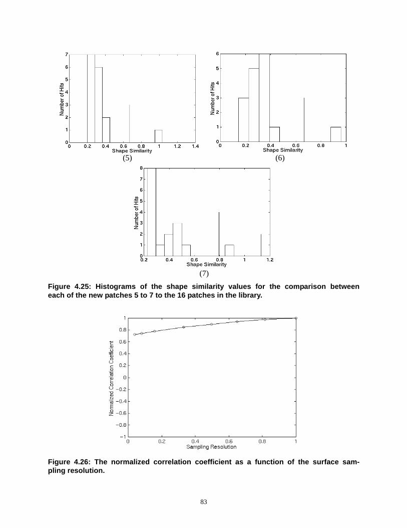
83


Figure 4.26: The normalized correlation coefficient as a function of the surface sam-pling resolution.

(5) (6)

(7)

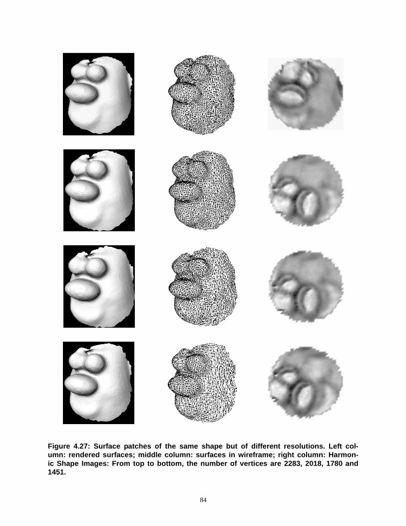
84

Figure 4.27: Surface patches of the same shape but of different resolutions. Left col-umn: rendered surfaces; middle column: surfaces in wireframe; right column: Harmon-ic Shape Images: From top to bottom, the number of vertices are 2283, 2018, 1780 and1451.

85

Figure 4.28: Surface patches of the same shape but of different resolutions. Left col-umn: rendered surfaces; middle column: surfaces in wireframe; right column: Harmon-ic Shape Images: From top to bottom, the number of vertices are 960, 491, 243 and 122.

86

Figure 4.29: The histogram of the shape similarity values for the pair comparison in thepatch library with new patches of different resolutions added.


(1) (2)

(3) (4)

87


Figure 4.32: The normalized correlation coefficient as a function of surface samplingresolution.

(5) (6)

(7)

88

remain exactly the same under occlusion. The best thing that can be done is to make thechange in representation gradual as occlusion increases. Therefore, the matching performedusing the representation degrades gracefully without any sudden failure due to a small amountof occlusion. This characteristic is called the robustness with respect to occlusion.

The reason for the robustness of Harmonic Shape Images with respect to occlusion lies in theway in which the boundary mapping is constructed. Recall that the construction of harmonicmaps consists of two steps: boundary mapping and interior mapping. The boundary mappingis used as a constraint for computing the interior mapping. Therefore, the change in boundarymapping affects the resultant harmonic image.

In order to handle occlusion that may occur on the boundary of the underlying surfacepatches, special attention is paid when constructing the boundary mapping. Recall from Sec-tion 2.4 that the boundary vertices are classified into radius boundary vertices and occlusionboundary vertices. It is the radius boundary vertices that determine the anglesai, which thendetermine the overall boundary mapping. Based on this, the occlusion boundary vertices arethen mapped to the interior of the unit disc instead of to its boundary according to the ratio oftheir surface distances to the central vertex and the radius of the surface patch (this ratio isreferred as distance ratio for the rest of the section). It is important to map the occlusionboundary vertices onto the interior of the unit disc because those vertices are, in fact, interiorvertices of the surface patch when there is no occlusion. If, instead, those occlusion verticesare mapped onto the boundary of the unit disc, there will be severe distortion in the boundarymapping, which in turn, will result in the distortion on the interior mapping.

By mapping the occlusion boundary vertices onto the interior of the unit disc using the dis-tance ratio, the effect of occlusion is limited within the occlusion range; therefore, it does notpropagate much outside of the occlusion range. This means that, as long as there are enoughradius boundary vertices present in the surface patch, the overall harmonic image will remainapproximately the same in spite of the occlusion. Figure 4.33 is an example to illustrate how theboundary mapping handles occlusion.

In Figure 4.33, a complete surface patch is shown in (a1). Its Harmonic Shape Images generatedwith and without using the distance ratio are shown in (a2) and (a3), respectively. Since there isno occlusion, there is little difference between those two images. The surface patch shown in Fig-ure 4.33(b1) is the patch in (a1) with occlusion. It can be seen that, using the distance ratio, itsHarmonic Shape Image (b2) is very similar to the non-occluded one(a2). In addition, the occlu-sion is present in the Harmonic Shape Image as well. In contrast, without using the distance ratio,the occlusion cannot be represented in the Harmonic Shape Image(b3). Compared with the non-occluded version in (a3), the distortion is significant.

In order to verify the robustness of Harmonic Shape Images, the following experiment is con-ducted. Among the surface patches in the patch library shown in Figure 4.5 and Figure 4.6, thefirst patch (Figure 4.5(1)) is selected. Different parts of that patch are removed manually to simu-late occlusion, resulting in seven new patches. These new patches are added to the patch library.As before, pair comparison among all the patches in the library is conducted. The expected resultis that the patches with occlusion should be identified as having the same shape as that of the firstpatch. Figure 4.34 and Figure 4.35 show the patches with occlusion and their Harmonic Shape

89

Images. The results of pair comparison are shown in Figure 4.36. Figure 4.36(a) shows that, inaddition to the high correlation values on the diagonal, the correlation values for patches 17 to 23compared with the first patch are also high. The patches numbered from 17 to 23 are the patcheswith occlusion. The correlation values for the pair comparison among the occlusion patches arehigh as well. This result shows that the Harmonic Shape Images of the patches with occlusion stillremain similar to the Harmonic Shape Image of the first patch. Figure 4.36(b) shows the matrix ofthe shape similarity values for the pair comparison among all the patches in the library. Thematrix has a similar distribution to that in Figure 4.36(a). Figure 4.36 shows the change of the nor-malized correlation coefficient as the boundary occlusion increases. As discussed above, the moreocclusion there is on the boundary, the more change there will be on Harmonic Shape Images.The curve in Figure 4.36 verifies this observation. It should be noted that, in this example, the cor-relation coefficient still remains very high when the percentage of boundary occlusion increasesto 50%. The reason for this is that the most significant features in the surface patch remain almostintact in all the occlusion patches, and there is small variation in shape in other parts of the surfacepatch. Occlusion occurs mainly in those parts of the patch with small shape variation. Figure 4.38and Figure 4.39 show the histogram of each occlusion patch compared with the 16 patches in thelibrary. In all the 7 cases, the first patch is identified as the qualified match.

Figure 4.33: Illustration of how to handle occlusion using the boundary mapping. (a1)A complete surface patch; (a2), (a3) Harmonic Shape Images of (a1) obtained with/with-out using the distance ratio; (b1) the surface patch in (a1) with occlusion; (b2), (b3) harmon-ic Images of (b1) obtained with/without using the distance ratio.

(a1) (a2) (a3)

(b1) (b2) (b3)

90

Figure 4.34: Patches with occlusion and their Harmonic Shape Images.

91

Figure 4.35: Patches with occlusion and their Harmonic Shape Images.

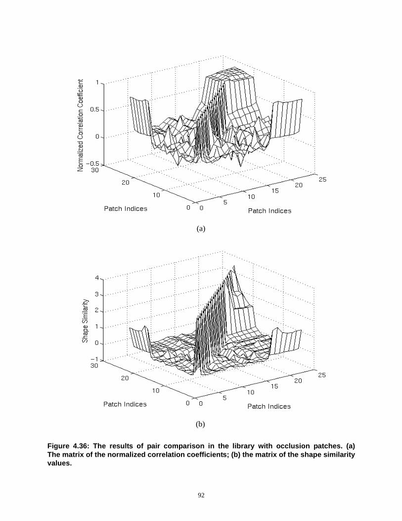
92

Figure 4.36: The results of pair comparison in the library with occlusion patches. (a)The matrix of the normalized correlation coefficients; (b) the matrix of the shape similarityvalues.

(a)

(b)

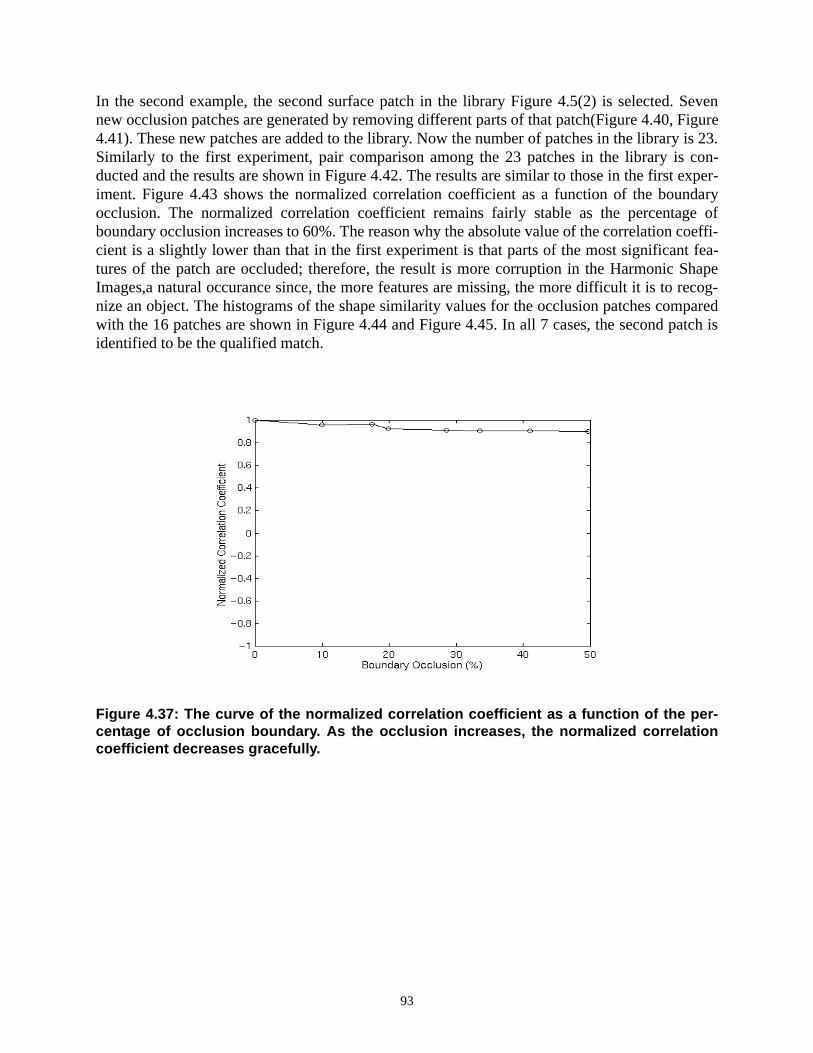
93

In the second example, the second surface patch in the library Figure 4.5(2) is selected. Sevennew occlusion patches are generated by removing different parts of that patch(Figure 4.40, Figure4.41). These new patches are added to the library. Now the number of patches in the library is 23.Similarly to the first experiment, pair comparison among the 23 patches in the library is con-ducted and the results are shown in Figure 4.42. The results are similar to those in the first exper-iment. Figure 4.43 shows the normalized correlation coefficient as a function of the boundaryocclusion. The normalized correlation coefficient remains fairly stable as the percentage ofboundary occlusion increases to 60%. The reason why the absolute value of the correlation coeffi-cient is a slightly lower than that in the first experiment is that parts of the most significant fea-tures of the patch are occluded; therefore, the result is more corruption in the Harmonic ShapeImages,a natural occurance since, the more features are missing, the more difficult it is to recog-nize an object. The histograms of the shape similarity values for the occlusion patches comparedwith the 16 patches are shown in Figure 4.44 and Figure 4.45. In all 7 cases, the second patch isidentified to be the qualified match.

Figure 4.37: The curve of the normalized correlation coefficient as a function of the per-centage of occlusion boundary. As the occlusion increases, the normalized correlationcoefficient decreases gracefully.

94

Figure 4.38: Histogram of the shape similarity values for the occlusion patches 1through 4 compared with the 16 patches in the library.

(1) (2)

(3) (4)

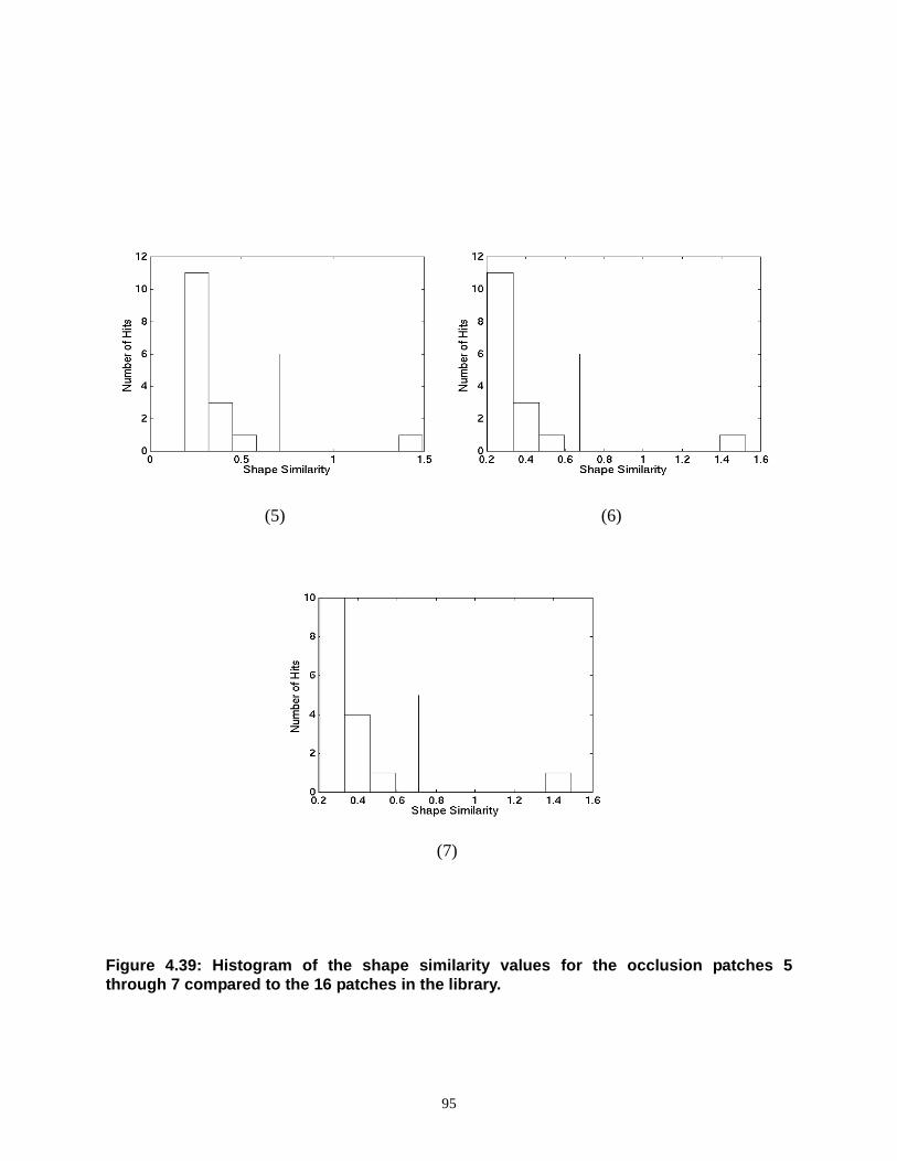
95

Figure 4.39: Histogram of the shape similarity values for the occlusion patches 5through 7 compared to the 16 patches in the library.

(5) (6)

(7)

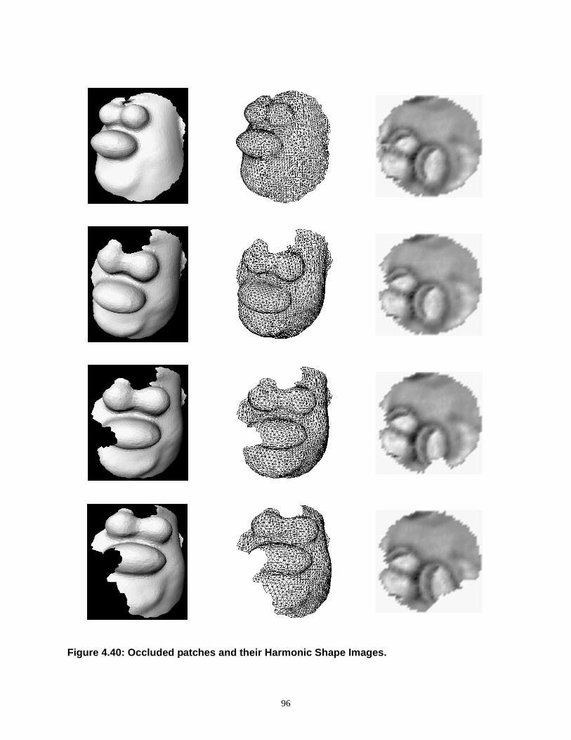
96

Figure 4.40: Occluded patches and their Harmonic Shape Images.

97

Figure 4.41: Occluded patches and their Harmonic Shape Images.

98

Figure 4.42: The results of pair comparison in the library with occlusion patches. (a)The matrix of the normalized correlation coefficients; (b) the matrix of the shape similarityvalues.

(a)

(b)

99

Figure 4.43: The curve of the normalized correlation coefficient as a function of the per-centage of occlusion boundary. As the occlusion increases, the normalized correlationcoefficient decreases gracefully.

Figure 4.44: Histogram of the shape similarity values for the occlusion patches 1through 4 compared with the 16 patches in the library.

(1) (2)

(3) (4)

100

Figure 4.45: Histogram of the shape similarity values for the occlusion patches 5through 7 compared to the 16 patches in the library.

(5) (6)

(7)

101

Chapter 5

Enhancements of Harmonic Shape Images

The generation, matching and experimental analysis of Harmonic Shape Images have beendiscussed in previous chapters. In this chapter, some enhancements of Harmonic ShapeImages will be discussed; these include dealing with missing data and improving the matchingresult of Harmonic Shape Images in the presence of noise.

5.1 Dealing with Missing Data

We have seen in Chapter 2 that, in order to compute the Harmonic Shape Image of a given surfacepatch, that patch needs to be a connected region without holes. In practice, this topology require-ment may not be satisfied because of the topology of the underlying surfaces, the occlusioncaused by other surfaces in the scene or missing data due to sensor errors. In other words, somesurface patches may have holes. In order to compute Harmonic Shape Images for those surfaces,an interpolation strategy is proposed and then explained in detail in this section. In the following,the effects of missing data on harmonic images is discussed first followed by the explanation ofhow to triangulate a surface patch that has missing data. Then Harmonic Shape Images obtainedusing the triangulation strategy are presented.

Effects of missing data on harmonic images

The idea of the interpolation strategy is to triangulate the holes resulting from missing data.Before presenting the interpolation algorithm, let us look at how missing data affect the com-putation of harmonic image for a given surface patch. This also explains why such an interpo-lation algorithm is necessary.

Multiple Boundaries: Two surface patches of the same shape are shown in Figure 5.1. The dif-ference between the two surface patches is that the one in Figure 5.1(a) does not have holes whilethe one in Figure 5.1(b) does. Recall the procedure of computing the harmonic image for a givensurface patch. The procedure consists of the following steps:

• Locate the boundary vertices of the surface patch• Construct the boundary mapping• Compute the spring constant for each interior edge of the surface patch• Construct the interior mapping

Since we have made the assumption about the surface patches to be orientable two-dimen-sional manifold, the boundary vertices of the surface patch in Figure 5.1(a) can be easily detectedby checking the number of triangles with which every edge is associated. Those boundary verticesare then re-ordered to construct a closed boundary for the surface patch. However, if a surfacepatch has holes (Figure 5.1(b)), then an extra step needs to be taken in order to determine whichclosed boundary is the outside boundary of the surface patch. This is the first effect of missingdata on the computation of harmonic images.

102

Under the assumption that the holes are relatively small with respect to the entire surfacepatch and the boundaries of the holes are simple curves in the three-dimensional space, i.e.,there are no twists, the outside boundary of a surface patch with holes can be determined bychecking the shortest path from the central vertex to each of the boundary vertices. In general,the inside boundaries block the shortest paths between the central vertex and some of the out-side boundary vertices; the opposite is not true, however. Therefore, none of the inside bound-ary vertices has the outside boundary vertices on its shortest path. Based on this fact, theoutside boundary is the one whose vertices have no other boundary vertices on its shortestpath to the central vertex.

Change of Spring Constants:Once the outside boundary has been determined, the boundarymapping can be computed. Using the boundary mapping as a constraint, the interior verticesare mapped onto the interior of the 2D target domain by minimizing the energy of a springsystem. This spring system is constructed by associating a spring with each interior edge ofthe surface patch. Computing the spring constant of each interior edge is an important step inconstructing the spring system. Recall from previous sections that the spring constantkij of anedgeeij is defined as

(5.1)

in which the anglesθ are defined in Figure 5.2:

According to (5.1), the spring constant of an interior edge has two terms because the edge is asso-ciated with two triangles. When the surface patch has holes, the spring constants of the interioredges that are on the hole boundaries have only one term. Although the spring constants of thoseedges are different from that without holes, the construction of the energy functional of the inte-rior mapping is not affected. However, as can be seen from Figure 5.3, the resultant harmonicimage of the interior vertices is affected.

Figure 5.1: Two surface patches of the same shape with (a) and without (b) holes.

(a) (b)

kij ctgθ emi emj,( ) ctgθ eli elj,( )+=

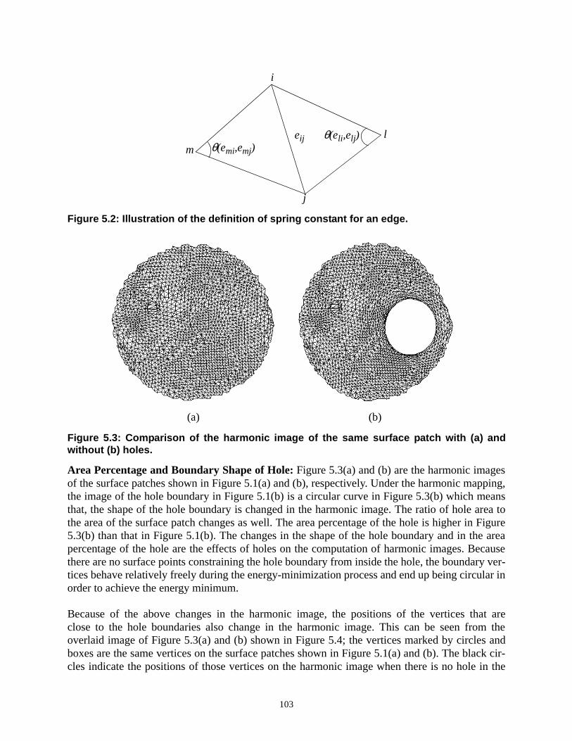
103

Area Percentage and Boundary Shape of Hole:Figure 5.3(a) and (b) are the harmonic imagesof the surface patches shown in Figure 5.1(a) and (b), respectively. Under the harmonic mapping,the image of the hole boundary in Figure 5.1(b) is a circular curve in Figure 5.3(b) which meansthat, the shape of the hole boundary is changed in the harmonic image. The ratio of hole area tothe area of the surface patch changes as well. The area percentage of the hole is higher in Figure5.3(b) than that in Figure 5.1(b). The changes in the shape of the hole boundary and in the areapercentage of the hole are the effects of holes on the computation of harmonic images. Becausethere are no surface points constraining the hole boundary from inside the hole, the boundary ver-tices behave relatively freely during the energy-minimization process and end up being circular inorder to achieve the energy minimum.

Because of the above changes in the harmonic image, the positions of the vertices that areclose to the hole boundaries also change in the harmonic image. This can be seen from theoverlaid image of Figure 5.3(a) and (b) shown in Figure 5.4; the vertices marked by circles andboxes are the same vertices on the surface patches shown in Figure 5.1(a) and (b). The black cir-cles indicate the positions of those vertices on the harmonic image when there is no hole in the

Figure 5.2: Illustration of the definition of spring constant for an edge.

Figure 5.3: Comparison of the harmonic image of the same surface patch with (a) andwithout (b) holes.

eij

i

j

ml

θ(emi,emj)θ(eli ,elj)

(a) (b)

104

surface patch. In contrast, the black boxes indicate the positions of the same vertices on the har-monic image when there is a hole in the surface patch. Figure 5.4 shows that for the vertices thatare close to the hole boundary, there is significant difference between their positions on the twoharmonic images. This difference gradually decreases as the vertices are further and further awayfrom the hole boundary.

Positions of Boundary VerticesWhen comparing the boundary images in Figure 5.3(a) and (b),we notice that the two boundary images differ in those vertices that have a hole boundary on theirshortest paths to the central vertex. Recall that the position of each boundary vertex in the har-monic image is determined by the angle between two consecutive radius vectors and the length ofthe shortest path between that vertex and the central vertex. While hole boundaries do not changethe angle between two radius vectors, they do change the lengths of the shortest paths between thecentral vertex and some of the outside boundary vertices. This is another effect that holes have onthe computation of harmonic images.

The goal of the strategy for handling missing data is to minimize the above effects on har-monic images resulting from missing data. The strategy is discussed in detail in the followingsection.

Triangulation of The Hole

Since there are no data in the hole area, the most direct solution is to fit a plane to the hole andtriangulate it. The complete hole interpolation algorithm consists of the following steps:

• Fit a plane to the hole• Project the vertices on the hole boundary onto the plane• Triangulate the polygon on the plane formed by the vertices on the hole boundary• Project the vertices in the planar triangulation to the 3D space• Update the surface patch

The first step is straightforward. Steps two to five are described in detail in the following.

Projection of Hole Boundary VerticesDenote the plane fit to the hole asP. Figure 5.5 illustrateshow to project the vertices on the hole boundary onto the fitting planeP. In Figure 5.5,vi is a ver-tex on the hole boundary andvi

’ is its projection on the best-fit planeP. N is the normal ofP andvmeanis defined in (5.3).vi

’ can be computed using (5.2) and (5.3). An example of hole boundaryand its projection onto the fit plane is shown in Figure 5.6.

(5.2)

(5.3)

The fit plane is then rotated so that it is parallel to the X-Y plane. The result is that, the z values ofthe vertices on the hole boundary become zero. This transformation can be expressed in (5.4), inwhich R represents the rotation matrix from the fit plane to the X-Y plane.

v′i

vi vmean– αN–=

α vi vmean–( ) N vmean,⋅ 1n--- hi

i 0=

h

= =

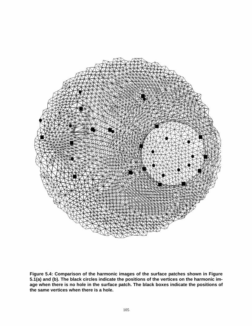
105

Figure 5.4: Comparison of the harmonic images of the surface patches shown in Figure5.1(a) and (b). The black circles indicate the positions of the vertices on the harmonic im-age when there is no hole in the surface patch. The black boxes indicate the positions ofthe same vertices when there is a hole.

106

(5.4)

Planar Triangulation After the vertices on the hole boundary are projected onto the fit plane,a program called Triangle is used to triangulate those vertices.

The program Triangle is a C program for two-dimensional mesh generation and constructionof Delaunay triangulations, constrained Delaunay triangulations and Voronoï diagrams. It isdeveloped by J. Shewchuk at Carnegie Mellon University[70]. Figure 5.7 shows an applicationexample of the Triangle program. A Planar Straight Line Graph(PSLG) is shown in Figure 5.7(a).Triangulating such a PSLG requires that the line segments in the original PSLG be the same linesegments in the final triangulation. In fact, this is the same requirement in our case when triangu-lating the holes because the hole boundary which consists of a sequence of straight line segmentsactually constructs a PSLG. Using theConstrained Delaunay triangulationfunction in the Trian-gle program, the PSLG in Figure 5.7(a) is triangulated as shown in Figure 5.7(b).

One issue with performing a constrained Delaunay triangulation is that some skinny triangleswith large aspect ratios may appear in the triangulation(Figure 5.7(b)). In order to address thisissue, Triangle has another function calledconforming Delaunay triangulation. This triangulationof a PSLG is a true Delaunay triangulation in which each PSLG segment may have been subdi-vided into several edges by the insertion of additional points, called Steiner points. These points

Figure 5.5: Projection of vertices on the hole boundary onto the best-fit plane.

Figure 5.6: An example of hole boundary (a) and its projection (b) onto the best-fitplane.

Pvmean

vi

vi’

N

(a) (b)

v′′i

Rv′i

=

107

are necessary to allow the segments to exist in the mesh while maintaining the Delaunay property.Steiner points are also inserted to meet constraints on the minimum angle and maximum trianglearea. The second function of Steiner points is more important to our application because it canavoid triangles with large aspect ratios. The result of triangulating Figure 5.7(a) using Conform-ing Delaunay triangulation is shown in Figure 5.7(c). Quite a few steiner points are added to theedges of the original PSLG. The resultant triangles in Figure 5.7(c) have much better aspect ratiosthan those in Figure 5.7(b).

Using theconforming Delaunay triangulationfunction of Triangle, the hole boundary shownin Figure 5.6(b) is triangulated and shown in Figure 5.8. The vertices in the interior of the hole arenew; there were created by Triangle in order to ensure quality triangles with good aspect ratios.

Figure 5.7: An application example of the Triangle program. (a) A Planar Straight LineGraph(PSLG); (b) the constrained triangulation of (a).

Figure 5.8: Triangulating Figure 5.6(a) using the conforming Delaunay triangulation func-tion of Triangle.

(a) (c)(b)

108

Back Projection of Hole Boundary Vertices From the discussion in the previous section, wecan see that new vertices may be created by the Triangle program. Since those new verticesare on the X-Y plane, they need to be projected back into the 3D space so that they can inter-polate the original surface patch. Based on the equations (5.2) and (5.4), the positions of the newvertices on the fit plane can be computed using (5.5).

(5.5)

Update of The Surface PatchAfter triangulating the holes in a given surface patch, new ver-tices, edges and triangles are created. Therefore, the original surface patch needs to beupdated by performing the following steps:

• Add the new vertices, edges and triangles to their respective lists• Update the topology information such as vertex-triangle, triangle-edge, edge-triangle,

triangle-triangle, etc.• Perform local retriangulation if necessary

It is straightforward to perform the first step by adding the new vertices, edges and triangles tothe existing arrays.

At the second step, updating the topology information means to update the connectivity infor-mation among the primitives of the surface patch. The primitives of a surface patch are verti-ces, edges and triangles. The triangles with which a vertex is associated are denoted as vertex-triangles. Similarly, the triangles with which an edge is associated are denoted as edge-trian-gles. Triangle-edge records the edges that construct a triangle. Triangle-triangle records theneighboring triangles of a triangle. When updating the topology information, special attentionshould be paid to the vertices, edges and triangles that are on the hole boundary because oldand new primitives interact on the boundary.

The third step is necessary only when original boundary edges are broken up into multipleline segments by theconforming Delaunay triangulationfunction of the Triangle program. Asexplained earlier in this section, in order to ensure quality triangles with good aspect ratios,the conforming Delaunay triangulationfunction may create new vertices. If some of the newvertices are on the edges of the hole boundary, then those edges will no longer exist. They arebroken up into new edges. This case is illustrated in Figure 5.9.

In Figure 5.9,vi, i=0...5 are vertices on the surface patch. The edges [v0, v1], [v1, v2], [v2, v3] and[v3, v0] construct the boundary of the hole. The verticesui, i=0...3 are the new vertices created bythe Triangle program. Since the new vertices are on the edges of the hole boundary, the originaledges [v0, v1] and [v2, v3] are replaced by new edges [v0, u0], [u0, u1], [u1, v1], [v2, u2], [u2, u3]and [u3, v3]. Other new edges are indicated by dash lines in Figure 5.9.

Although the hole is triangulated, the surface mesh is not a valid triangular mesh because ofthe new vertices on the hole boundary. In this case, local re-triangulation needs to be done inorder to maintain the original surface patch as a valid triangular mesh. In Figure 5.9, the dot linesegments indicate the new edges created by local re-triangulation. Similar to step 2, the topologyinformation of the surface patch needs to be updated after local re-triangulation.

vi new, R1–vi new,

′′vmean+=

109

Harmonic Image with Triangulation

After using the triangulation strategy to process a given surface patch with holes, the har-monic image of that surface patch can be computed. Figure 5.10(a) and (b) show the harmonicimages of the surface patches in Figure 5.1(a) and (b); respectively. The triangulated area is indi-cated by the arrow. Compared with Figure 5.3(b), the boundary mapping in Figure 5.10(b) isgreatly improved. Figure 5.11 shows the difference between the boundary mappings in Figure5.10(a) and (b) more clearly.

Figure 5.9: An example of broken edges on the hole boundary.

Figure 5.10: Harmonic images of the surface patches shown in Figure 5.1(a) and (b), re-spectively. (b) is obtained using the triangulation strategy.

u2

v5

v4

v3 v2

v1

v0

u3

u1u0

(a) (b)

Triangulatedarea

110

Using the hole triangulation strategy, the surface distance from the central vertex to each ofthe boundary vertices in Figure 5.1(a) is computed. All the values are stored in a vectord. Thesame distances are computed for the surface patch in Figure 5.1(b) and stored indh

t. The differ-ences betweend and dh

t are computed and displayed by the solid line in Figure 5.11. Withoutusing the triangulation strategy, the same distances are computed again for the patch in Figure5.1(b) and stored indh. The differences betweend anddh is displayed by the dashed line in Figure5.11. It can be seen that the differences are zero for both curves except for the vertices in the indexrange of [0, 10) and (145, 160] because those vertices have vertices on the hole boundary on theirshortest paths to the central vertex. For those boundary vertices, the differences are much smallerwhen using the hole triangulation strategy compared to not using it.

It should be noticed that the change of boundary mapping depends on the shape of the under-lying surface patch. Because the triangulation is actually a first-order approximation of themissing surface, it approximates the surface well when the missing surface has low curvature.

Based on the harmonic images, the Harmonic Shape Images of the surface patches in Figure5.1(a) and (b) are computed and displayed in Figure 5.12(a) and (b), respectively. The interpo-lated vertices are colored white to indicate that they are invalid for shape comparison. Moreexamples are shown in Figure 5.13 to illustrate the effectiveness of the triangulation strategy. The

Figure 5.11: Comparison of boundary mapping with and without using the hole triangu-lation strategy. The unit of the vertical axis is the radius of the 2D unit disc.

111

correlation coefficients between the surface patch in Figure 5.1(a) and each of the patches withmissing data in Figure 5.1(b) and Figure 5.13 are computed; and the results are 0.996446,0.993301 and 0.992507, respectively. This quantitatively demonstrates how well Harmonic ShapeImages can handle missing data.

5.2 Cutting And Smoothing

In Section 4.3 and 4.4, it has been discussed and demonstrated that Harmonic Shape Images arerobust with respect to sampling resolution and occlusion. In order to further enhance their robust-ness so that the matching result will be more accurate, cutting and smoothing are used to pre-pro-cess the Harmonic Shape Images before matching them.

Recall the construction of boundary mapping for generating Harmonic Shape Images in Chapter2. Given a surface patch, its boundary vertices can be classified into radius boundary vertices andocclusion boundary vertices according to the surface distance from each boundary vertex to thecentral vertex of the surface patch. This means that the occlusion parts of the surface patch can beexactly located before comparison. Considering the fact that most distortion on Harmonic ShapeImages appears around the occlusion boundary, discounting the corresponding pixels in thoseareas when comparing the images should help obtain the correct matching result. In our imple-mentation, this technique is referred as cutting. Smoothing is also applied to the Harmonic ShapeImages before matching in order to decrease the distortion caused by resolution and occlusion. Inour implementation, Gaussian smoothing is used with . The implementation of cuttingand smoothing is further explained using the example in Figure 4.40.

Figure 5.14(a), (b) and (c) show the surface patch and its Harmonic Shape Image on the third rowof Figure 4.40. After applying cutting and smoothing on (c), the resultant Harmonic Shape Imageis shown in Figure 5.14(d). The normalized correlation coefficient between the occluded patchand the original patch (shown in the first row of Figure 4.40) increases from 0.759951 to0.854042. Using the cutting and smoothing techniques, the second experiment on occlusion (Fig-

Figure 5.12: The Harmonic Shape Images of the surface patches in Figure 5.1(a) and (b),respectively. (b) is computed using the triangulation strategy.

(a) (b)

σ 0.25=

112

Figure 5.13: Examples of using the triangulation strategy to compute the HarmonicShape Images of surface patches with holes.

113

ure 4.40 and Figure 4.41) is repeated and the results are presented as follows. Figure 5.15 showsthe curves of normalized correlation coefficient as a function of the occlusion boundary with andwithout applying cutting and smoothing. Clearly, the comparison of the two curves shows that,with the help of cutting and smoothing, the correlation coefficient improves as the boundaryocclusion increases.

Although smoothing can help decrease the distortion caused by resolution and occlusion, thesmoothing parameterσ cannot be specified too large because large smoothing eliminates featuresof surface patches and causes different patches to appear similar. To verify that cutting andsmoothing do not introduce confusion in surface matching, the occluded patches in Figure 4.40and Figure 4.41 are compared with all the 16 patches in the second patch library. As before, paircomparison among all the patches is performed and the matrices for the normalized correlationcoefficients and shape similarity are shown in Figure 5.16(a) and (b), respectively. The histogramof the shape similarity values for each occluded patch compared with the 16 patches is shown inFigure 5.17. These results further demonstrate how the occluded patches can be distinguishedfrom other patches with the help of cutting and smoothing.

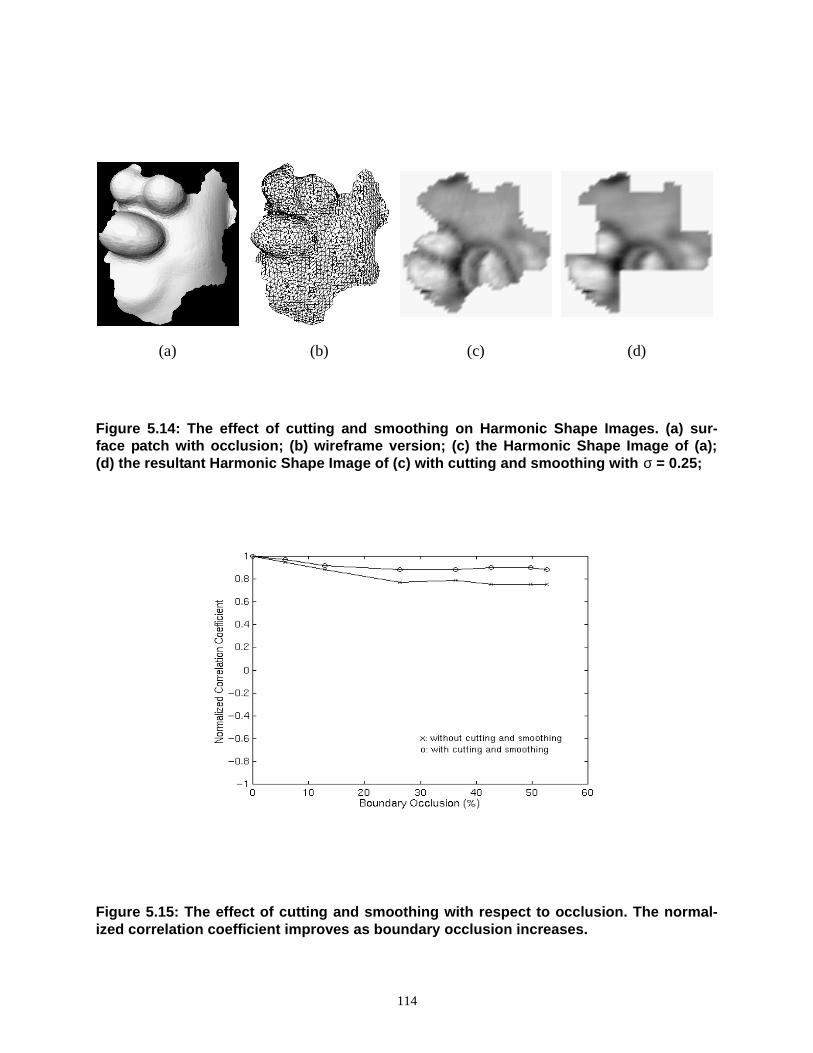
114

Figure 5.14: The effect of cutting and smoothing on Harmonic Shape Images. (a) sur-face patch with occlusion; (b) wireframe version; (c) the Harmonic Shape Image of (a);(d) the resultant Harmonic Shape Image of (c) with cutting and smoothing with σ = 0.25;

Figure 5.15: The effect of cutting and smoothing with respect to occlusion. The normal-ized correlation coefficient improves as boundary occlusion increases.

(a) (b) (c) (d)

115

Figure 5.16: The results of pair comparison in the library with occlusion patches. (a)The matrix of normalized correlation coefficients; (b) the matrix of shape similarity values.

(a)

(b)

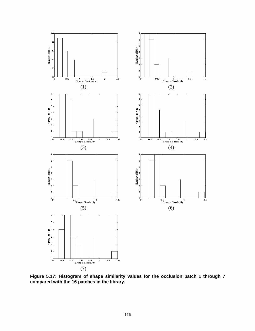
116

Figure 5.17: Histogram of shape similarity values for the occlusion patch 1 through 7compared with the 16 patches in the library.

(1) (2)

(3) (4)

(5) (6)

(7)

117

Chapter 6

Additional Experiments

In this chapter, the results of additional experiments on surface matching using Harmonic ShapeImages are presented. The experiments include surface registration for face modeling and meshwatermarking, accuracy test for surface registration and object recognition in scenes with occlu-sion. These additional experiments are presented to further demonstrate the usefulness of Har-monic Shape Images in different applications of surface matching. The algorithms and strategiesin those examples can be incorporated into a surface matching system in the future, althoughbuilding a complete system is not addressed at this time.

6.1 Surface Registration for Face Modeling

Face modeling has received more and more attention in the vision and graphics fields due to itsimportant role in the medical area, e.g., plastic surgery. Systems that can capture accurate 3Dgeometry and high quality color surface data along with software that can provide accurate facemodels can aid the surgeons in various ways. For example, it is possible to measure distance andarea on 3D models; it is practical to track recovery, growth and degenerative conditions by directcomparison of 3D models; it is possible to objectively compare the effects of alternative treat-ments by comparing the 3D models.

In the experiments of face modeling, the range images are provided by the research group led byProfessor Shizhuo Yin in the Electrical Engineering Department of Pennsylvania State Univer-sity. Typically, each data set consists of three images of either a human face or the face of a mask:one front view along with two side views. Each of the two side views has about 40% overlap withthe front view. There is no prior knowledge about the transformation among any of the rangeimages. An example face data set is shown in Figure 6.1.

The example set shown in Figure 6.21 is used to illustrate the registration process. In Figure 6.2,The front and left range images are first registered. Some of the statistics of the meshes are listedin Table 6.1. Because the meshes are of high resolution, a hierachical approach is used to performthe registration (discussed in Chapter 3) for experimental purposes. A number of vertices areselected randomly on both the front and the left images so that those vertices are distributed asevenly as possible. Some of the selected vertices are shown in Figure 6.3. The number of ran-domly selected vertices on the front and left images are denoted asnfront andnleft. Surface patchesare created using those vertices as central vertices; the radius of the surface patches is selected tobe 40.0. The radius is determined based on the following mesh information. The area of the sur-face patch is selected to be 20% of the overlapping area of the two images. The area of the over-lapping part of the two images is estimated using the average of the areas of the two meshesmultiplied by the estimated overlapping percentage, about 40% in this case. Assuming that thesurface patch is a disc, the radius can be calculated once the area of the disc is known.

1. The range images were taken from a mask instead of a human face in this example.

118

Figure 6.1: An example set of the face range images. First row: the rendered view of theright, front and left images; second row: the wireframe of the right, front and left images.

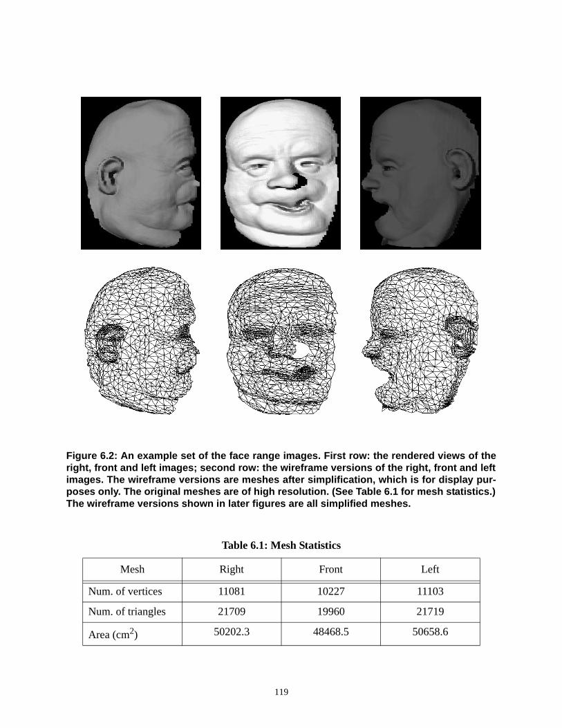
119

Figure 6.2: An example set of the face range images. First row: the rendered views of theright, front and left images; second row: the wireframe versions of the right, front and leftimages. The wireframe versions are meshes after simplification, which is for display pur-poses only. The original meshes are of high resolution. (See Table 6.1 for mesh statistics.)The wireframe versions shown in later figures are all simplified meshes.

Table 6.1: Mesh Statistics

Mesh Right Front Left

Num. of vertices 11081 10227 11103

Num. of triangles 21709 19960 21719

Area (cm2) 50202.3 48468.5 50658.6

120

After surface patches are created on both meshes, a validity checking step is performed. A surfacepatch is considered to be valid when satisfying the following requirements.

• Topology

If the surface patch has holes in it, then those holes are triangulated. If none of the esti-mated area of the holes exceeds 5% of the total area of the surface patch, then the topol-ogy requirement is considered to be satisfied.

• Occlusion

If the angle for any occlusion range is larger thanα * π, then the patch is considered tohave too much occlusion, therefore not satisfying the occlusion requirement.α is aparameter determined by the application. In general, in the case of surface registration,the patches that are on the boundary of meshes tend to have more occlusion. Accordingly,α is set to be 0.375, making the threshold of the angle for the occlusion range equal to67.5 degrees.

After the validity check, the number of valid surface patches on the front and left meshes isn’front

andn’left. The Harmonic Shape Images are created for each of the valid patches. The comparison

is performed by matching each Harmonic Shape Image on the front mesh to all the HarmonicShape Images on the left mesh. Alltogether, there aren’front x n’left number of comparisons to beperformed.

Recall that the issue of surface matching using Harmonic Shape Images has been discussed inChapter 3. When given two surfaces to be matched,m surface patches were randomly selected onthe first surface while only one surface patch was selected on the second surface. The process ofsearching for the best-matched patch for the patch on the second surface was explained in detail.In practice, considering the fact that, on the first surface, there may not be a match for a randomlyselected patch on the second surface. In this case, more surface patches need to be selected on thesecond surface. That is what has been done in the above face modeling example. There, the prin-

Figure 6.3: Randomly selected vertices on the front and left images.

121

ciple of searching for the best-matched patch for any one patch is the same as that explained inChapter 3. The difference is that, because there may be multiple good matches, one more stepneeds to be taken in order to determine which match is the best one. This extra step is explainedbelow.

After the comparison of Harmonic Shape Images on both meshes, the result for each patch on thefront mesh compared with all the patches on the left mesh is analyzed using the fourth-spread sta-tistical method which was discussed in Chapter 3. The following are some examples of the result-ant histograms of the comparison results.

Figure 6.4: An example of patch comparison results between the front mesh and the leftmesh. The Harmonic Shape Image of the surface patch on the front mesh is compared tothe Harmonic Shape Images of all the selected valid patches on the left mesh. The histo-gram of the shape similarity values is shown on the right. One qualified match on the leftmesh is found which is shown by overlapping it on the left mesh. It should be noticed that,in this case, the shape similarity value of the best-matched patch is just above the thresh-old.

122

In Figure 6.4, the histogram of the shape similarity values shows that there is one qualified match(above the threshold) on the left mesh for the patch on the front mesh. The two matched patchesare shown by overlapping them on the front and left meshes, respectively. The shape similarityvalue of the qualified match is just above the threshold. In Figure 6.5, the histogram shows a qual-ified match whose shape similarity value is well above the threshold. This fact shows that the sur-face patch on the front mesh is well distinguished from the patches on the left mesh. In Figure 6.6,no qualified matches are found according to the histogram because all the shape similarity valuesare below the threshold.

The examples in Figure 6.4, Figure 6.5 and Figure 6.6 are representatives of then’front x n’leftpatch comparison results between the front mesh and the left mesh. Two issues should be broughtup regarding the comparison results. Let us define the surface patches on the front mesh to bescene patches and those on the left mesh to be model patches. The first issue is to select the patchwhich should be used to perform the search on the left mesh. The second issue is that more thanone scene patches found their qualified matches among the models patches, which pair ofmatched patches should be used to compute the transformation between the two meshes. The dis-cussion on the above two issues is as follows.

Figure 6.5: An example of patch comparison results between the front mesh and the leftmesh. The Harmonic Shape Image of the surface patch on the front mesh is compared tothe Harmonic Shape Images of all the selected valid patches on the left mesh. The histo-gram of the shape similarity values is shown on the right. One qualified match on the leftmesh is found which is shown by overlapping on the left mesh. In this case, the shape sim-ilarity value of the best-matched patch is well above the threshold.

123

Selecting Scene Patches

It is true that there are many possible scene patches on the front mesh. In fact, every vertex on thefront mesh can be used as a central vertex to generate a scene patch using the specified radius.However, not every one of these scene patches can find its qualified match on the left mesh,because meshes only partly overlap. In general, there are two types of scene patches that may beable to find their matches among the model patchesl The ones in the overlapping region are theregistration-correct matches for which we are looking. Others outside the overlapping region areregistration-incorrect matches caused by local shape similarity of the two surfaces, e.g., symme-try. Because there is no prior knowledge about the overlapping region, it is impossible to select ascene patch in that region searching for its best match among the model patches. The solution tothis problem is to use a number of randomly selected scene patches. The patches in the overlap-ping region have equal chance to be selected as other patches.

Figure 6.6: An example of patch comparison results between the front mesh and the leftmesh. The Harmonic Shape Image of the surface patch on the front mesh is compared withthe Harmonic Shape Images of all the selected valid patches on the left mesh. The histo-gram of the shape similarity values is shown on the right. In this case, no qualified matchis found because all the shape similarity values are below the threshold.

124

Selecting the Best Match for Computing Transformation

The second question is that, among all the qualified matches, which pair of patches should beused to compute the transformation? The solution to this problem is to define a discriminabilityvalued(p, Ω) between a surface patch and a set of surface patches according to the histogram ofthe shape similarity values.d(p,Ω) is defined in (6.1).

(6.1)

In (6.1),p denotes a surface patch,Ω denotes the set of surface patches being compared top. C(p,q) denotes the shape similarity value between the Harmonic Shape Images ofp andq. The firstterm on the right-hand side is the maximum of the shape similarity value; the second term is thethreshold for the qualified matches. When the discriminability valued(p,Ω) is positive and large,the best matchq in Ω of p can be well identified fromΩ. Whend(p, Ω) is positive and small, thebest matchq in Ω of p can be identified but with less discriminability than the case in whichd(p,Ω) is positive and large. Whend(p, Ω) is negative, no qualified match is found. Based on theabove definition, the pair of matched surface patches with the largest discriminability valueshould be used to compute the transformation between the two meshes.

The matches in the above example with positive discriminability values are shown in Figure 6.7.Some of the matched surface patches along with their Harmonic Shape Images are shown in Fig-ure 6.8. The one on the last row is a mis-match. Among all the matched surface patches, five ofthem are correct matches. Their discriminability values are shown in circles in Figure 6.7. Someanalysis that has been done regarding the matching result is presented below.

Figure 6.7: The matches on the two surfaces in Figure 6.3 with positive discriminability val-ues.

d p Ω,( ) max C p q,( ) q Ω∈( ) Threshold C p q,( ) q Ω∈( )–=

125

The Match with the Largest Discriminability Value

The matched patches shown on the second row of Figure 6.8 constitute a correct match. Its dis-criminability value is the largest in Figure 6.7. Therefore, the transformation between the two sur-faces should be computed using the correspondences on the two matched surface patches.

Patches with More Features vs. Patches with Fewer Features

Figure 6.8 shows that the matched patches are rich in shape variation. This justifies the observa-tion that patches with more features are more easily identified among a group of surface patches.This also shows that Harmonic Shape Images represent those shape variations well.

Interpreting Mis-matches

There is a mis-match on the last row of Figure 6.8. It should be noted that the mis-matches are notcorrect in the sense of using them to compute the transformation between the two surfaces. In thesense of matching Harmonic Shape Images, the mis-matchesare correct because they are similarin shape. This is the case for the mis-matches in Figure 6.8. Mis-matches occur because surface

Figure 6.8: Matched surface patches on the two surfaces in Figure 6.3 with positive dis-criminability values.

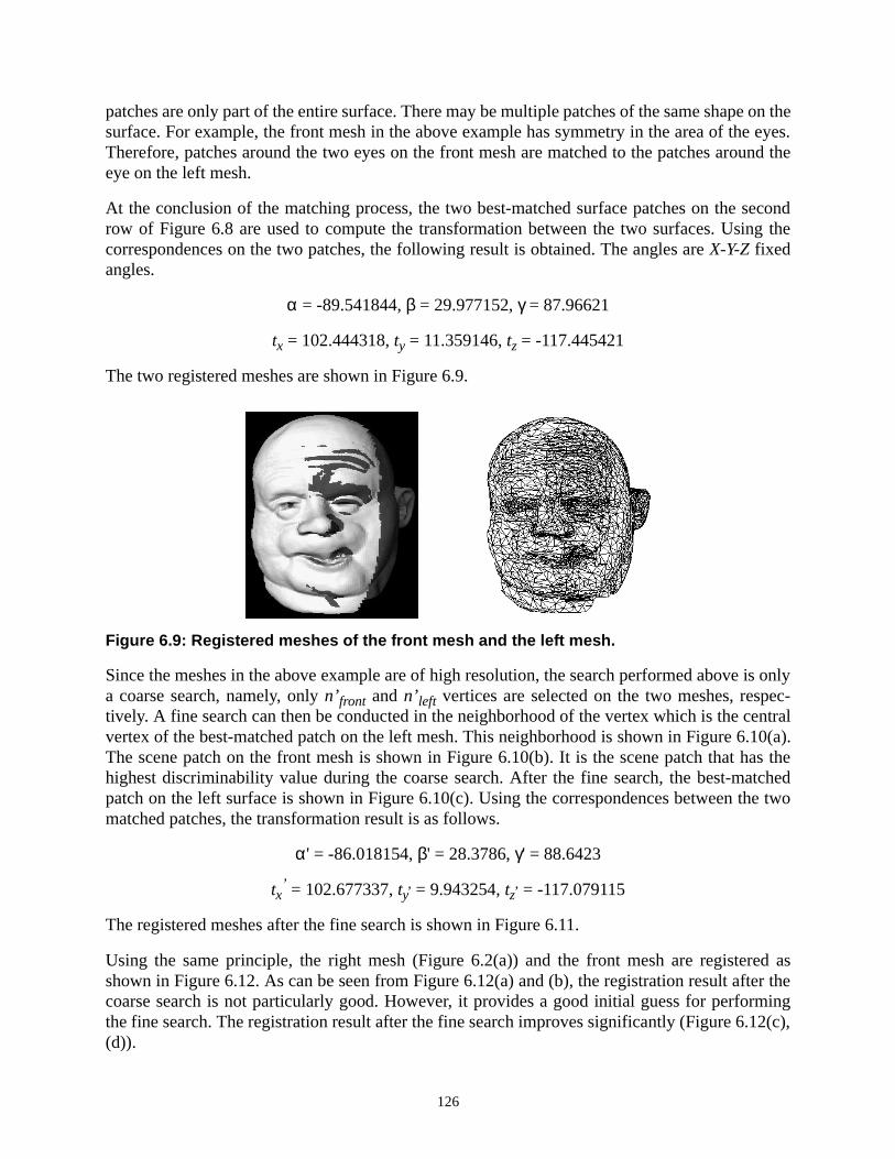
126

patches are only part of the entire surface. There may be multiple patches of the same shape on thesurface. For example, the front mesh in the above example has symmetry in the area of the eyes.Therefore, patches around the two eyes on the front mesh are matched to the patches around theeye on the left mesh.

At the conclusion of the matching process, the two best-matched surface patches on the secondrow of Figure 6.8 are used to compute the transformation between the two surfaces. Using thecorrespondences on the two patches, the following result is obtained. The angles areX-Y-Z fixedangles.

α = -89.541844,β = 29.977152,γ = 87.96621

tx = 102.444318,ty = 11.359146,tz = -117.445421

The two registered meshes are shown in Figure 6.9.

Since the meshes in the above example are of high resolution, the search performed above is onlya coarse search, namely, onlyn’front and n’left vertices are selected on the two meshes, respec-tively. A fine search can then be conducted in the neighborhood of the vertex which is the centralvertex of the best-matched patch on the left mesh. This neighborhood is shown in Figure 6.10(a).The scene patch on the front mesh is shown in Figure 6.10(b). It is the scene patch that has thehighest discriminability value during the coarse search. After the fine search, the best-matchedpatch on the left surface is shown in Figure 6.10(c). Using the correspondences between the twomatched patches, the transformation result is as follows.

α' = -86.018154,β' = 28.3786,γ' = 88.6423

tx’ = 102.677337,ty

, = 9.943254,tz, = -117.079115

The registered meshes after the fine search is shown in Figure 6.11.

Using the same principle, the right mesh (Figure 6.2(a)) and the front mesh are registered asshown in Figure 6.12. As can be seen from Figure 6.12(a) and (b), the registration result after thecoarse search is not particularly good. However, it provides a good initial guess for performingthe fine search. The registration result after the fine search improves significantly (Figure 6.12(c),(d)).

Figure 6.9: Registered meshes of the front mesh and the left mesh.

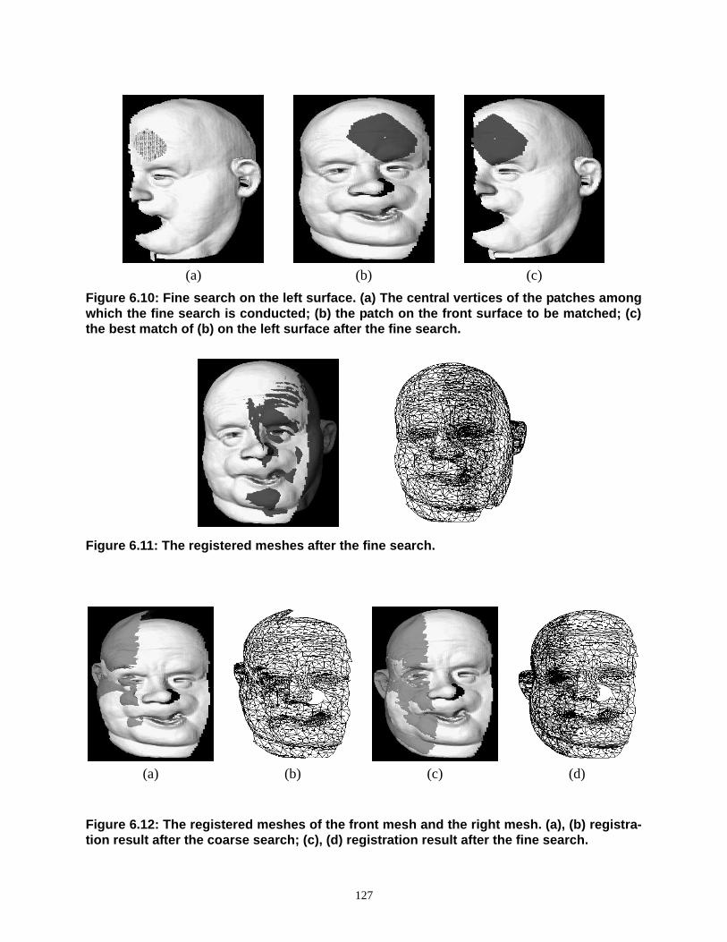
127

Figure 6.10: Fine search on the left surface. (a) The central vertices of the patches amongwhich the fine search is conducted; (b) the patch on the front surface to be matched; (c)the best match of (b) on the left surface after the fine search.

Figure 6.11: The registered meshes after the fine search.

Figure 6.12: The registered meshes of the front mesh and the right mesh. (a), (b) registra-tion result after the coarse search; (c), (d) registration result after the fine search.

(a) (b) (c)

(a) (b) (c) (d)

128

Using a mesh integration program described in [46], the three registered meshes (Figure 6.13(a))are integrated into a single mesh (Figure 6.13(b), (c), (d)).

The registration and integration results for the meshes in Figure 6.1 are shown in Figure 6.14.

Figure 6.13: Mesh integration. (a) The three registered meshes to be integrated; (b), (c) and(d) the front, left and right views of the integrated mesh.

Figure 6.14: Mesh integration. (a) The three registered meshes to be integrated; (b), (c) and(d) the front, left and right views of the integrated mesh.

(a)

(b)

(c)

(d)

(a) (b) (c) (d)

129

6.2 Registration in mesh watermarking

An approach was proposed by Dr. H. Hoppe in [62] to watermarking triangular meshes. Water-marking provides a mechanism for copyright protection of digital media by embedding informa-tion identifying the owner in the data. The piece of embedded information is called watermark.Robust watermarks are able to survive a variety of attacks, including transformation, scaling,cropping, smoothing, simplification and resampling. The watermarking process proposed in [62]is as follows.

A watermark vectorw is selected using the information inherent to the original meshM. Then thewatermark,w, is inserted intoM using some basis functions defined onM. The watermarked meshis denoted asMwatermark. As a result of this insertion, the 3D position of each vertex onM hasgone through a different linear transformation in the following form.

(6.2)

In (6.2),vx’ are the X coordinates of the vertices on the watermarked meshMwatermark. vx are the

coordinates of the vertices on the original meshM. ε is a user-provided global parameter that con-trols the energy of the watermark.Φ is a nxmmatrix which has scalar basis functionsφi

j as col-umns.di is a global displacement vector associated with verticesvj. The matrixhdx is a diagonalmatrix which represents the weighted (byhi) X coordinate of the displacementdi. w is the water-mark vector. Equation (6.2) shows that the effect of the watermark coefficientwi is to perturb theeach vertexvj by a vector proportional towiφi

jdi. Meanwhile, the connectivity among the verticesdoes not change. Of course, the transformation needs to be small enough so that the appearance ofM does not change visually. An example original mesh and its watermarked version are shown inFigure 6.15 (All the mesh models shown in this subsection are provided by Dr. H. Hoppe ofMicrosoft Research).

Figure 6.15: An example mesh (a), (b) and its watermarked version (c), (d).

vx′ vx

ε Φ

h1d1x

… …hmdmx

w+=

(a) (b) (c) (d)

130

When a suspect meshMsuspectis obtained, it is first registered to the original meshM in the samecoordinate frame. ThenMsuspectis resampled so that the resultant meshMr

suspecthas the sameconnectivity as that of the original meshM. At the next step, the difference between the 3D coor-dinates of each pair of the corresponding points onMr

suspectandM is taken. The watermark vec-tor w’ is extracted from the above residuals. At the final step, a statistical method is used todetermine whetherw andw’ are the same.

It can be seen from the above watermarking algorithm that the registration of the suspect meshMsuspectto the original meshM is crucial to the extraction of the watermark from the suspectmesh. If the registration is not accurate enough, then the extracted watermarkw’ will not be accu-rate enough in order to match the true watermarkw. In [62], the registration algorithm proposed in[14] which required good initial estimate of the underlying transformation was used. Some userintervention was also necessary as reported in [62].

Because the registration problem in watermarking triangular meshes is actually a special case of3D surface matching, Harmonic Shape Images can be used to find the global transformation, fol-lowed by refinement using the ICP algorithms. An example is shown as follows.

An original mesh is shown in Figure 6.16(a) and (b). Figure 6.16(c) is an suspect mesh. Comparedwith the original mesh, the suspect mesh is simplified, cropped and transformed using a rigidtransformation. Some of the randomly selected vertices on the original mesh and the suspect meshare overlaid on both meshes (Figure 6.16(d), (e)). Using these vertices as centers and specifyingthe radius equal to 50.0, surface patches along with their Harmonic Shape Images are computed.Among all these, the best-matched patches are shown in Figure 6.16(f) and (g). Using that pair ofpatches, the transformation between the original and the suspect meshes is first computed andthen refined using ICP. The suspect mesh is aligned with the original mesh as shown in Figure6.16(h) and (i).

The most meaningful way to check the registration accuracy in mesh watermarking is to extractthe watermark from the aligned suspect mesh and compare the extracted watermark with the orig-inal watermark. The comparison result can tell us whether the registration is sufficiently accurate.Unfortunately, we do not have the software to perform the watermark extraction. Therefore, thefollowing method is used to check the registration accuracy.

Suppose that rigid transformation is the last operation that is applied to the original mesh to obtaina suspect mesh. Without applying rigid transformation, the suspect mesh stays aligned with theoriginal mesh. Although this alignment may not be the best one since the suspect mesh hasalready been changed from the original mesh to a different one, the alignment can be used as astarting point for the ICP algorithm to find a better alignmentT’ and a smaller alignment errorE’ .For the suspect meshes which have gone through rigid transformations, the registration errorETshould be comparable toET

’. For the example shown in Figure 6.16,E’ = 0.261163, andET’ =

0.241831; they are fairly close.

Figure 6.17 shows another registration example for mesh watermarking. The original mesh isshown in Figure 6.17(a) and (b). Figure 6.17(c) shows the suspect mesh which is simplified,cropped and transformed using a rigid transformation. Some of the randomly selected vertices onthe original mesh and the suspect mesh are overlaid on both meshes (Figure 6.17(d), (e)). Usingthese vertices as centers and specifying the radius equal to 1.5, surface patches are generated and

131

Figure 6.16: Harmonic Shape Images used in registration of the mesh watermarking pro-cess. (a), (b) Original mesh; (c) suspect mesh; (d) some of the randomly selected verticeson the original mesh; (e) some of the randomly selected vertices on the suspect mesh; (f),(g) the best matched patches overlaid on the original and the suspect meshes; (h), (i) thealigned suspect mesh with the original mesh.

(a) (b) (c)

(g) (h) (i)

(d) (e) (f)

132

their Harmonic Shape Images are then computed as well. Among all these patches, the best-matched patches are shown in Figure 6.17(f) and (g). Using that pair of patches, the transforma-tion between the original and the suspect meshes is first computed and then refined using ICP. Thesuspect mesh is aligned with the original mesh as shown in Figure 6.17(h) and (i). The registrationerror for this example is 0.044202, as compared with the reference error 0.044516. Again, the twoerrors are close.

6.3 Accuracy Test of Surface Registration Using Harmonic Shape Images

One important issue with surface registration is the registration result’s degree of accuracy. Dueto the difficulties in obtaining ground truth, even if the measurement of the registration accuracycan be conducted, the confidence of that accuracy still depends on how accurate the ground truthis. In order to conduct the best accuracy test using the hardware equipment available in our lab,the following experiments were designed.

An object with free-form surfaces is selected and markers are attached to the object. For example,Figure 6.18 shows a white bunny with red dots painted on it. Two range images along with textureimages can be taken of the object from different viewing directions as shown in Figure 6.18. Themarkers are present in both range images (texture images as well) because the two range imagesoverlap. Therefore, the fact that those markers are the same physical points in 3D space can beused as ground truth to measure the registration accuracy as long as those markers can be identi-fied in the two range images.

The two texture images taken by the sensor are used to locate the markers in the range images.The process is as follows. At the first step, the corresponding red markers are manually picked inthe two texture images. The texture coordinates of those markers are recorded. Then, by searchingfor the same texture coordinates as the markers among the vertices in the two range images, thecorresponding pair of points in 3D space can be located. Those pairs of 3D points are used asground truth to test the registration accuracy.

A few practical issues about the above operation need to be discussed. These issues are directlyrelated to how accurate the ground truth is. First, each red marker in the texture image maps to afew pixels instead of to only one pixel. Second, the resolution of the texture image is much higherthan that of the range image. For example, the resolution of the texture images in Figure 6.18 is400x400, and the number of vertices in the range images in Figure 6.18 is fewer than 4500 in bothcases. What the second issue means is that, for any particular pixel in the texture image, there maynot be a corresponding vertex in the range image. In this case, the fact that the size of each markeris a few pixels can help us find a corresponding vertex in the range image for each marker in thetexture image. Figure 6.19 further illustrates this idea.

In Figure 6.19,N(c, m) is a small neighborhood in a texture image that represents a marker.c,selected mannually, is the center of the neighborhood. The size ofN(c, m)is (2m+1)x(2m+1) inwhich m is determined according to the actual size of the marker. For each pixel inN(c, m), itscorrespondence is searched through the texture coordinates of all the vertices in the range image.As a result, a few vertices may be found as shown in Figure 6.19. Those vertices are in a smallneighborhood denoted byN’ . After N’ is located, the average of all the vertices inN’ is used as thecorrespondence of the marker in the texture image.

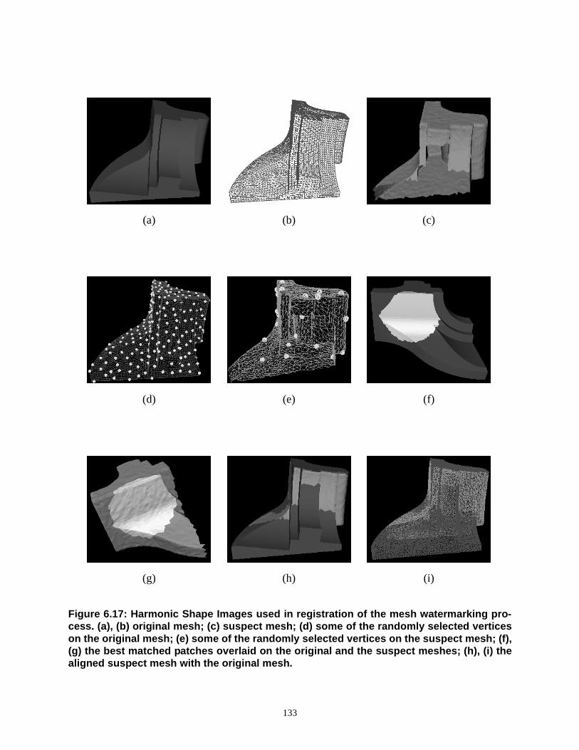
133

Figure 6.17: Harmonic Shape Images used in registration of the mesh watermarking pro-cess. (a), (b) original mesh; (c) suspect mesh; (d) some of the randomly selected verticeson the original mesh; (e) some of the randomly selected vertices on the suspect mesh; (f),(g) the best matched patches overlaid on the original and the suspect meshes; (h), (i) thealigned suspect mesh with the original mesh.

(a) (b) (c)

(g) (h) (i)

(d) (e) (f)

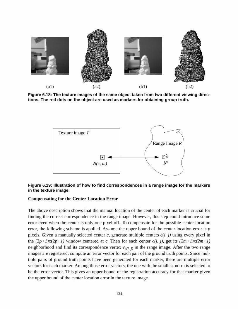
134

Compensating for the Center Location Error

The above description shows that the manual location of the center of each marker is crucial forfinding the correct correspondence in the range image. However, this step could introduce someerror even when the center is only one pixel off. To compensate for the possible center locationerror, the following scheme is applied. Assume the upper bound of the center location error isppixels. Given a manually selected centerc, generate multiple centersc(i, j) using every pixel inthe (2p+1)x(2p+1) window centered atc. Then for each centerc(i, j), get its (2m+1)x(2m+1)neighborhood and find its correspondence vertexvc(i, j) in the range image. After the two rangeimages are registered, compute an error vector for each pair of the ground truth points. Since mul-tiple pairs of ground truth points have been generated for each marker, there are multiple errorvectors for each marker. Among those error vectors, the one with the smallest norm is selected tobe the error vector. This gives an upper bound of the registration accuracy for that marker giventhe upper bound of the center location error in the texture image.

Figure 6.18: The texture images of the same object taken from two different viewing direc-tions. The red dots on the object are used as markers for obtaining group truth.

Figure 6.19: Illustration of how to find correspondences in a range image for the markersin the texture image.

(a1) (b1)(a2) (b2)

Texture imageT

Range ImageR

N(c, m) N’

135

According to the strategy discussed above, the result of the registration accuracy test for theexample in Figure 6.18 is presented below. Table 6.2 shows the manually selected centers for the9 markers in the texture images shown in Figure 6.18. Considering the fact that the number of pix-els is about 28,000 (for the object only in the texture image) and the number of vertices in therange image is about 4,500, on average, there are about 6 pixels in the texture image correspond-ing to one vertex in the range image. Therefore, the size ofN(c, m)is selected to be 9 withm=1.The corresponding vertices found for each marker are shown in Figure 6.20.

Assuming the upper bound for center location error on the texture image isp=1 pixel, the registra-tion error for each marker is shown in Table 6.3. Each value is the norm of the error vectorbetween the corresponding markers in the two range images. The unit of the measurements is themillimeter. The average registration error is 0.3986. The resolution of a range image is defined tobe the mean of the edge lengths. For the two range images in Figure 6.18, the resolution is about2mm. Therefore, the relative registration error is one-fifth of the mesh resolution.

Table 6.2: The texture coordinates of the manually selected centers for the markers

Marker Index Coordinates in Texture ImageT1 Coordinates in Texture ImageT2

1 (216, 232) (190, 232)

2 (248, 214) (217, 215)

3 (228, 248) (201, 248)

4 (243, 268) (215, 267)

5 (244, 277) (214, 279)

6 (243, 289) (213, 289)

7 (212, 355) (186, 354)

8 (244, 351) (213, 350)

9 (224, 382) (195, 380)

Table 6.3: Registration error for each marker

Marker 1 2 3 4 5 6 7 8 9

Error 0.3177 0.4194 0.0909 0.3471 0.6252 0.1797 0.4811 0.7983 0.3280

136

6.4 Object Recognition in Scenes with Occlusion

In this section, Harmonic Shape Images are used to recognize objects in scenes with occlusion.The goal of the experiments is to demonstrate the usefulness of Harmonic Shape Images in thisapplication. The recognition strategy in this section is for experimental purposes although it couldbe incorporated into a complete recognition system in the future. In the following, the construc-tion of the object library will be introduced first, followed by the explanation of the hypothesize-and-test recognition strategy. Then the experimental results will be presented along with an analy-sis of those results.

Object Library

The object library consists of four objects as shown in Figure 6.21, where only the front part ofeach object is used to create the models. This is because there is not much shape variation in otherparts of each object. Some vertices on each object are randomly selected as central vertices togenerate model surface patches. Those selected vertices are distributed as uniformly as possibleon each object. It is not necessary to create surface patches for all the vertices on each objectbecause the sampling resolution is high and surface patches created by neighboring vertices aresimilar in shape. Some of the central vertices of the model surface patches are overlaid on eachobject and shown in Figure 6.21(a3), (b3), (c3) and (d3). The radius is selected to be 25.0. Thearea of each model surface patch is about 10 to 15 percent of the area of each object. HarmonicShape Images are generated for each of the model surface patches and are stored in the objectlibrary.

Figure 6.20:Corresponding markers on the two range images which were taken from differ-ent viewing directions.

12

3

4

6

87

9

5

12

34

56

7 8

9

137

It should be noticed that the objects shown in Figure 6.21(a1), (b1) and (d1) are similar in shape.Compared with using objects of distinct shape in the recognition experiment, this similaritymakes the recognition tasks more difficult. The success of the experiment will not only demon-strate the application of Harmonic Shape Images in object recognition, but will also justify its dis-criminability of different shapes, even for surfaces without much shape variation.

Scene Processing

Figure 6.22 shows a scene with occlusion. As shown in the texture image in Figure 6.22(a), thebackground of the scene is black. This helps the range finder in our lab increase the depth of theview. The meshes in Figure 6.22(c) and (d) show that, although the object on the left is occludedby the right object, the two objects do not touch each other. Scene processing is a hypothesize-and-test process in which a decision is made about each connected region in a scene on whether itmatches any of the objects in the library. In this section, the steps for hypothesis generation arefirst discussed, followed by discussion of the test process.

Hypothesis GenerationThe first step in hypothesis generation is to apply smoothing operationon the scene in order to remove sampling noise. Then, some vertices are randomly selected in thescene mesh to generate scene surface patches. Because of the high resolution of the mesh in thescene, it is not necessary to generate a large amount of surface patches. Some of the selected ver-tices are shown in Figure 6.22(b). Using them as central vertices and specifying the radius equalto 25.0, the scene surface patches are created and their Harmonic Shape Images are generated. Atthe third step, the scene Harmonic Shape Images are compared with each set of model HarmonicShape Images in the library.

Recall that Harmonic Shape Images can be created only on connected surfaces. This characteristicmeans that in the application of object recognition, each connected region in the scene should beexamined independently. Matching hypotheses should be generated for each connected regionaccording to its matching scores to the objects in the library. Table 6.4 summarizes the matchingstatistics for all the connected regions in the scene in Figure 6.22.

.As shown in the last row of Table 6.4, the number of selected scene surface patches is 146. Thetotal number of matched scene patches to each set of model patches is shown as the numerator inthe last row of Table 6.4. For each connected region, the number of matched patches to eachmodel and the number of selected patches are listed in the first and second rows. The central ver-tices of those matched scene and model patches are shown in Figure 6.24.

For each connected region and a model in the library, the generation of the matching hypothesis isdetermined by the ratio ofnr

m andnr in whichnrm is the number of matched surface patches to the

model andnr is the number of selected patches in that region. This ratio is called matching scoreand denoted asλ(ri, mj) in which ri denotes theith region in the scene andmj denotes thejthmodel in the library. Whenλ(ri, mj) is above a thresholdλcutoff, a hypothesis is generated on thematching of regioni and modelj.

138

Figure 6.21: Objects in the model library for the recognition experiments.

(a1)

(a2)

(a3)

(b1)

(b2)

(b3)

(c1)

(c2)

(c3)

(d1)

(d2)

(d3)

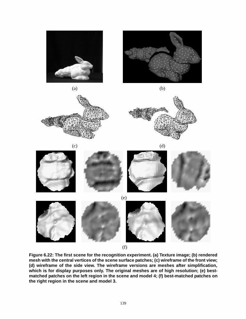
139

Figure 6.22: The first scene for the recognition experiment. (a) Texture image; (b) renderedmesh with the central vertices of the scene surface patches; (c) wireframe of the front view;(d) wireframe of the side view. The wireframe versions are meshes after simplification,which is for display purposes only. The original meshes are of high resolution; (e) best-matched patches on the left region in the scene and model 4; (f) best-matched patches onthe right region in the scene and model 3.

(a) (b)

(c) (d)

(e)

(f)

140

Selectingλcutoff The selection ofλcutoffdepends on two considerations. The first one comes fromthe local property of Harmonic Shape Images, which are local representations of surface patches.In general, they can describe the shape of only part of a given surface. Considering the fact thattwo surfaces of different shapes may be similar at a few regions, using only one pair of matchedsurface patches is not reliable in determining whether those two surfaces are similar. Therefore,for each connected region and a model in the library, among the selected surface patches in theregion there should be a fair amount of matched patches to the model. This consideration deter-mines the lower bound ofλcutoff.

The second consideration when selectingλcutoffcomes from the fact that there may be clutter inthe scene. Clutter can result in a connected region with different objects. Under this situation, thematched patches in the region correspond to different models in the library. Therefore, for anyone of those models, the matching score of the region,λ(ri, mj), may not be as high as that whenthe connected region consists of only one object. This consideration poses the upper bound forλcutoff.

Based on the above two considerations,λcutoff is set to 10% empirically. In fact, this value isintentionally set low so as not to miss potential matches.

After usingλcutoff equal to 10% to threshold the matching scores in Table 6.4, three hypothesescan be made about the region-model matches (the values greater thanλcutoff are underlined inTable 6.4). Denote the connected region on the left in the scene (Figure 6.22) as region 1 and theone on the right as region 2, the three hypotheses are as follows:

1. Region 1 matches model 42. Region 2 matches model 13. Region 2 matches model 3

Among the above three hypotheses, the second one is generated becauseλcutoff is set low. Theverification process would show that this hypothesis will be rejected.

Hypothesis TestThe test process consists of four steps. The first is to compute the transformationbetween the matched region and the model. The transformation is then applied so that both ofscene and the model are in the same coordinate system. The second step is to use the IterativeClosest Point (ICP) algorithm to refine the transformation obtained in the first step. At the thirdstep, the hypothesis is accepted or rejected based on the alignment error computed by the ICP

Table 6.4: Summary of the Recognition Experiment for Scene 1

Region/Model Model1 Model2 Model3

Region1 2/37 0/37 1/37

Region2 13/109 5/109 82/109

Total Matches 15/146 5/146 83/146

141

Figure 6.23: Matching results of scene 1 to each object in the library.

(a1) (a2) (a3) (a4)

(b1) (b2)

(c1) (c2) (c3) (c4)

(b1) (b2) (b3) (b4)

142

algorithm. If the hypothesis is accepted, then at the fourth step, the distance to the model surfaceis computed for each vertex in the scene region. Each distance value is thresholded in order todetermine whether it is on the model surface. This is actually a segmentation step which segmentsthe matched scene object from a cluttered scene.

Following the above four steps, the test result of the scene in Figure 6.22 is shown in Figure 6.24.The alignment results obtained by using Harmonic Shape Images are shown in Figure 6.24(a1),(b1) and (c1). The refined alignment results are shown in (a2), (b2) and (c2). The alignment errorafter the ICP for each hypothesis is listed in Table 6.5. The alignment error for the second hypoth-esis is significantly larger than that of the other two. In fact, the threshold for the alignment erroris selected to be half of the resolution of the mesh in the scene. In this case, it is 0.867135. There-fore, the first and third hypotheses are accepted and the second one is rejected. Models 1 and 4 arealigned with the scene as shown in Figure 6.25.

Two other recognition examples are shown in Figure 6.26 and Figure 6.27. The regions in eachscene are numbered from left to right sequentially. The matching scores are listed in Table 6.6 andTable 6.8 with the values greater thanλcutoffunderlined. Table 6.7 and Table 6.9 list the alignmenterrors for both scenes. The mesh resolutions for the two scenes are 1.84543 and 1.8381, respec-tively. In both cases, all the connected regions are recognized correctly and all the alignmenterrors are less than half of the mesh resolution.

Table 6.5: Alignment Error for Each Hypothesis in Scene1

Hypothesis 1 2 3

Error 0.160898 3.02334 0.439101

Table 6.6: Matching Scores for Scene2

Region/Model Model1 Model2 Model3 Model4

Region1 1/57 3/57 2/57 11/57

Region2 3/60 43/60 0/60 2/60

Region3 0/54 2/54 41/54 6/54

Total Matches 4/171 48/171 43/171 19/171

Table 6.7: Alignment Errors for Regions in Scene2

Region 1 2 3

Error 0.783502 0.190562 0.382581

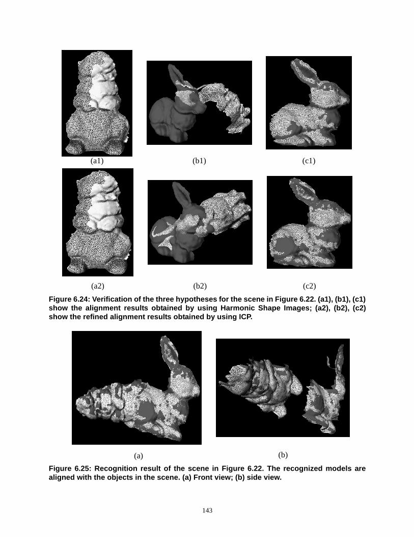
143

Figure 6.24: Verification of the three hypotheses for the scene in Figure 6.22. (a1), (b1), (c1)show the alignment results obtained by using Harmonic Shape Images; (a2), (b2), (c2)show the refined alignment results obtained by using ICP.

Figure 6.25: Recognition result of the scene in Figure 6.22. The recognized models arealigned with the objects in the scene. (a) Front view; (b) side view.

(a1)

(a2)

(b1)

(b2)

(c1)

(c2)

(a) (b)

144

Figure 6.26: Recognition example. (a) The texture image of the scene; (b) the mesh of thescene in wireframe; (c) the central vertices of the selected scene surface patches; (d) therecognized models aligned with their corresponding regions in the scene. The wireframeversions are meshes after simplification, and are for display purposes only. The originalmeshes are of high resolution.



Region1 19/41 0/41 0/41 2/41

Region2 1/82 4/82 11/82 81/82

Region3 1/43 34/43 2/43 1/43

Total Matches 21/166 38/166 13/166 84/166

Table 6.9: Alignment Errors for Regions in Scene3

Region 1 2 3

Error 0.391074 0.15994 0.250005

(a) (b)

(c) (d)

145

A fourth scene is shown in Figure 6.28. The matching scores and alignment errors are listed inTable 6.10 and Table 6.11, respectively. The first region in the scene does not match any of themodels in the library, although it is supposed to match the fourth one. In this case, not being ableto match scene and model is due to the lack of features in the first region. In fact, the upper part ofmodel 4 which consists of rich shape information, is occluded by the second object in the scene.Except for the first region, the other three regions are correctly recognized, and all the alignmenterrors are less than half of the mesh resolution which is 1.78922.




Region1 0/18 0/18 0/18 0/18

Region2 0/59 42/59 1/59 1/59

Region3 0/22 2/22 0/22 13/22

(a) (b)

(c) (d)

146

Region4 1/58 4/58 25/58 4/58

Total Matches 1/157 48/157 26/157 18/157

Table 6.11: Alignment Errors for Scene4

Region 1 2 3 4

Error - 0.12362 0.37545 0.425999




(a) (b)

(c) (d)

147

A fifth scene is shown in Figure 6.29. The interesting point about this scene is that the secondobject in the scene does not belong to the object library. The recognition result shows that it wasnot mis-matched to any of the objects in the library. The other two objects are correctly identifiedand aligned. The resolution of the mesh in the scene is 1.9706.



Region1 1/59 2/59 26/59 1/59

Region2 2/58 1/58 4/58 8/58

Region3 2/77 3/77 1/77 49/77

Total Matches 5/194 6/194 31/194 58/194

Table 6.13: Alignment Errors for Scene5

Region 1 2 3

Error 0.232193 - 0.329847


(a) (b)

(c) (d)

149

Chapter 7

Future Work

In this thesis, a new and novel representation for 3D free-form surfaces, which is called HarmonicShape Images, has been proposed, analyzed and demonstrated by some practical applications. Aspart of the future work, some extensions of Harmonic Shape Images are first discussed in thischapter. These extensions further demonstrate the novel properties of Harmonic Shape Imagesand its advantages when being used in surface matching. The second part of the future workfocuses on the application of Harmonic Shape Images in shape analysis which is not addressed inthis thesis. As a geometric representation which preserves both the shape and continuity of theunderlying surfaces, Harmonic Shape Images provide a powerful tool for performing shape anal-ysis.

7.1 Extensions to Harmonic Shape Images

In addition to the properties of Harmonic Shape Images and the matching strategy using thoseimages that have been discussed in the previous chapters, the following algorithmic additionscould be used to further improve the efficiency of Harmonic Shape Images in surface matching.

Finding the Rotation

Recall the generation of Harmonic Shape Images in Chapter 2. Because of the one-degree free-dom of the boundary mapping, Harmonic Shape Images could be different by a planar rotation forthe same surface patch. In the current implementation, the rotation is found by the direct search inthe angle space.

Different strategies could be used to speed up the rotation finding process. For example, an esti-mate of the rotation could be found using subsampled versions of the Harmonic Shape Images.The rotation could be refined at the full resolution of the Harmonic Shape Images. Another strat-egy would be to use a coarse-to-fine approach to search the angle space.

Cutting the Search Space

Performing correlation-based template matching is not the only way to compare two HarmonicShape Images. In fact, given a scene Harmonic Shape Image and a set of model Harmonic ShapeImages, the goal is to find the best match of the scene image among the model images. Thismeans that eliminating the model images that are not similar to the scene image will definitelyspeed up the search process.

Due to the fact that Harmonic Shape Images are a geometric representation for 3D free-form sur-faces, partial information about the underlying surfaces could be extracted from Harmonic ShapeImages. For example, histograms of the normalized shape distribution functions could be con-structed from those images. If two Harmonic Shape Images are quite different in the histogram,then they could be eliminated from the search space without further comparison.

150

Building a Surface Matching System

The experiments conducted in this thesis are for demonstration and verification of the propertiesand usefulness of Harmonic Shape Images in surface matching. Although the algorithms for gen-erating and matching Harmonic Shape Images are available now, a complete system for surfacematching has not yet been built up. More issues need to be addressed when integrating differentprograms into a complete system. For example, improving the efficiency of the system and auto-matically setting the thresholds in the matching process.

Harmonic Texture Images

In the current surface matching strategy using Harmonic Shape Images, only shape information isused. However, more surface information such as texture could easily be added to the matchingprocess because Harmonic Shape Images are geometric surface representations which preserveboth the shape and the continuity of the underlying surfaces. This representation provides a gen-eral framework for representing surface attributes such as shape and texture. Therefore, in addi-tion to creating Harmonic Shape Images, Harmonic Texture Images (HTIs) can be created bystoring the texture information on the harmonic images. HTIs are especially useful when compar-ing surfaces with few shape variations but rich texture variations. Unlike the previous surface rep-resentations that were designed only for representing shape, the generality of Harmonic ShapeImages enables the easy and natural addition of various information into the surface matchingprocess.

7.2 Shape Analysis and manipulation

As a representation for 3D free-form surfaces with novel properties, Harmonic Shape Images canbe used to conduct shape analysis and manipulate shapes. In this section, the future work on appli-cations of Harmonic Shape Images in shape similarity, surface reconstruction and shape synthesisis discussed.

Shape Similarity

Harmonic Shape Images are local surface representations; therefore, a single Harmonic ShapeImage can describe only part of the shape of a given surface. This is in contrast to the global rep-resentations, which can represent the shape of the entire surface. However, those global represen-tations usually have difficulties with objects of arbitrary topology. In this aspect, defining astatistical shape similarity measure using local representations could provide a way to comparesurfaces of arbitrary topologies.

Given two surfaces represented by triangular meshes, the same number of most shape significantsurface patches is selected on both of them according to their Harmonic Shape Images. Thoseselected patches are ranked according to their shape significance. By comparing two sets of Har-monic Shape Images with the same rank, a shape similarity measure can be obtained by combin-ing the pair comparison results of those images. This shape similarity measure is consistent withthe visual perception of human in the way that surfaces with similar most significant shape fea-tures are considered to be similar.

151

Surface Reconstruction

Similar to the Spherical Attribute Image (SAI) representation, it is possible to reconstruct theunderlying surface given its Harmonic Shape Image and a boundary constraint. This reconstruc-tion property comes from the fact Harmonic Shape Images preserve both the shape and the conti-nuity of the represented surfaces.

Shape Synthesis

Harmonic Shape Images can be used in shape synthesis first in the shape space and then back tothe range space. Synthesizing surfaces in the 3D space directly may be difficult due to the issuessuch as registration, scaling and different sampling resolutions. Harmonic Shape Images providea way to synthesize shape in the shape space, or in the HSI space. Different Harmonic ShapeImages can be morphed together using different combination functions. Then the correspondingsurfaces in 3D space can be reconstructed based on the reconstruction property of HarmonicShape Images.

153

Chapter 8

Conclusion

In this thesis, a novel geometric representation for 3D free-form surfaces is proposed. Due to theuse of the mathematical theory on harmonic maps, the representation is named Harmonic ShapeImages. The properties of those images are analyzed and applications of the images in surfacematching are demonstrated. The contributions of this thesis are summarized as follows.

• Matching surfaces by matching surface patches

The idea of matching surfaces by matching surface patches is proposed and implemented in thisthesis. Harmonic Shape Images, the novel representation for 3D free-form surfaces proposed inthis thesis, are the key to the success of patch-based surface matching. Unlike point-based match-ing, patch-based surface matching uses both the shape and the continuity information of theunderlying surfaces. Therefore, the establishment of the correspondences on the two surfacesbecomes trivial after patch-based matching is done.

• Harmonic Shape Images are intrinsic to the shape of the underlying surfaces

Due to the energy functional used in construction of the mapping between a 3D surface patch anda 2D planar domain, Harmonic Shape Images are intrinsic to the shape of the underlying surfacepatches. Therefore, surface patches of different shape have different Harmonic Shape Images, i.e.,the images are unique with respect to shape. This is an important property for surface representa-tion to be used to identify surfaces of different shape.

• Harmonic Shape Images preserve the continuity of the underlying surfaces

Due to the way Harmonic Shape Images are constructed, the continuity of the source surfacepatch is preserved exactly on the Harmonic Shape Image. This means that there is one-to-one cor-respondence between the points on the surface patch and the points on the Harmonic ShapeImage. In fact, the harmonic map is a parameterization of the surface patch onto the 2D planardomain. The property of continuity preservation facilitates the establishment of correspondencesafter two Harmonic Shape Images are determined to match each other. No heuristic-guided post-processing is needed in order to organize the matched pair of points into mutually consistent cor-respondences.

• Harmonic Shape Images provide a general framework for representing surface attributes

Harmonic Shape Images are a geometric representation which preserves both the shape and conti-nuity of the underlying surfaces. Therefore, any distribution functions defined on a surface patchcan be defined on its Harmonic Shape Image as well. In addition to shape, other distribution func-tions such as surface normals, colors, texture, material, can all be represented in the same way asHarmonic Shape Images. This general framework makes the use of other surface attributes, e.g.,texture, in surface matching easy and natural.

• Harmonic Shape Images are robust to surface sampling resolution and occlusion

154

Harmonic Shape Images’ ability to deal with surface sampling resolution lies in the property thatthose images are intrinsic to the underlying surfaces. As long as the sampling resolution is highenough to represent the underlying surfaces, the corresponding Harmonic Shape Images are accu-rate enough as well. Due to the way the boundary mapping is constructed, Harmonic ShapeImages are robust to occlusion. Experimental analysis has shown that the matching performanceof Harmonic Shape Images decreases gracefully as the sampling resolution decreases and theocclusion increases.

• Harmonic Shape Images are both discriminative and stable

Being an effective surface representation, Harmonic Shape Images are discriminative enough todistinguish among surface patches of different shapes. Meanwhile, their stability ensures that sur-face patches with similar shapes have similar Harmonic Shape Images. This property is especiallyuseful when applying the coarse-to-fine strategy to speed up the surface matching process. Exper-imental analysis has been conducted to verify the discriminability and stability of HarmonicShape Images.

• The use of Harmonic Shape Images has been demonstrated in different applications ofsurface matching

Harmonic Shape Images have been used in varying applications of surface matching includingview registration and object recognition in scenes with occlusion. Those extensive experimentsshow that, as a novel surface representation, Harmonic Shape Images not only have nice proper-ties, but they can also solve real world surface matching problems.

155

Bibliography

[1]A. Aho, J.E. Hopcroft and J.D. Ullman,Data structures and algorithms, Addison-Wesley,Reading, Mass., 1983.

[2]A. D. Aleksandrov, V.A. Zallgaller,Intrinsic geometry of surfaces, Translation of Mathemati-cal Monographs Series, AMS Publisher, 1967.

[3]F. Arman and J.K. Aggarwal, CAD-based vision: object recognition in cluttered range imagesusing recognition strategies,Computer Vision, Graphics and Image Processing, Vol.58, No. 1,pp.33-48, 1993.

[4]C.Bajaj, F. Bernardini and G. Xu, Automatic reconstruction of surfaces and scalar fields from3-D scans.Proc. Computer Graphics (SIGGRAPH’95), pp.109-118, August,1995.

[5]P. Belhumeur, J. Hespanha and D. Kriegman, Eigenfaces vs. Fisherfaces: recognition usingclass specific linear projection,Proc. European Conference on Computer Vision (ECCV’96),1996.

[6]R. Bergevin, D. Laurendeau and D. Poussart, Estimating the 3D rigid transfromation betweentwo range views of a complex object,11th IAPR, Int’l Conf. Patt. Recog.,pp. 478-482, TheHague, The Netherlands, Aug. 30 - Sep. 3, 1992.

[7]R. Bergevin, D. Laurendeau and D. Poussart, Registering range views of multipart objects,Computer Vision and Image Understanding, Vol.61, No.1, pp. 1-16, 1995.

[8]P.J. Besl, The free-form surface matching problem,Machine Vision for Three-dimensionalScenes, H. Freeman, ed., pp. 25-71, Academic Press, 1990.

[9]P.J. Besl, Triangles as a primary representation,Object Representation in Computer Vision, M.Hebert, J. Ponce, T. Boult and A. Gross, eds., pp. 191-206, Berlin, Springer-Verlag, 1995.

[10]P.J. Besl and N.D. Mckay, A method for registration of 3-D shapes,IEEE Transaction Patternon Pattern Analysis and Machine Intelligence,14(2): pp. 239-256, 1992.

[11]J. Boissonnat, Geometric structures for three-dimensional shape representation, ACM Trans.on Graphics, Vol.3, No.4, pp. 266-286, October 1984.

[12]N. Burgess, M. N. Granieri and S. Patarnello. 3-D object classification: application of a con-structive algorithm,International Journal of Neural Systems(Singapore), 2(4): pp. 275-282,1991.

[13]T. Cass, Polynomial-time geometric matching for object recognition,Int’l Jour. ComputerVision, Vol.21(1/2), pp. 37-61, 1997.

[14]Y. Chen and G. Medioni, Object modeling by registration of multiple range images,ImageVision Computing, 10(3): 145-155, 1992.

[15]Y. Chen and G. medioni, Surface description of complex objects from range images,Proc.IEEE Computer Vision and Pattern Recognition (CVPR’94), pp. 153-158, 1994.

156

[16]C.S. Chua and R. Jarvis, 3D free-form surface registration and object recognition,Int’l J. ofComputer Vision, Vol. 17, pp. 77-99, 1996.

[17]C.S. Chua and R. Jarvis, Point signatures: a new representation for 3D object recognition,Int’lJ. of Computer Vision, 25(1), pp.63-85, 1997.

[18]B. Curless and M. Levoy, A volumetric method for building complex models from rangeimages,Proc. Computer Graphics (SIGGRAPH’96), August 1996.

[19]H. Dellingette, M. Hebert and K. Ikeuchi, A spherical representation for the recognition ofcurved objects,Proc. Computer Vision and Pattern Recognition (CVPR’93), pp. 103-112, 1993.

[20]H. Dellingette, M. Hebert and K. Ikeuchi, Shape representation and image segmentation usingdeformable surfaces,Image and Vision Computing, Vol.10, No.3, pp. 132-144, 1992.

[21]H. Dellingette, M. Hebert and K. Ikeuchi, Representation and recognition of free-form sur-faces, Technical Report, CMU-CS-92-214, Computer Science Department, Carnegie MellonUniversity, November, 1992.

[22]J. Deovre,Probability and statistics for engineering and sciences, Brooks/Cole, Belmont, CA,1987.

[23]T. D. DeRose, M. Lounsbery, J. Warren, Multi-resolution analysis for surfaces of arbitrarytopological type, Technical Report, 93-10-05, Deptment of Computer Science and Engineering,University of Washington, October, 1993.

[24]D. Dion Jr., D. Laurendeau and R. Bergevin, Generalized cylinder extraction in range images,Proc. Int’l Conf. on Recent Advance in 3-D Digital Imaging and Modeling, Ottawa, pp. 141-147, May 1997.

[25]C. Dorai, A. Jain, COSMOS - a representation scheme for 3D free-form objects,IEEE Trans-action Pattern on Pattern Analysis and Machine Intelligence,19(10): pp. 1115-1130, 1997.

[26]M. Eck, T. DeRose, T. Duchamp, H. Hoppe, M. Lounsbery, and W. Stuetzle, Multi-resolutionAnalysis of Arbitrary Meshes, Technical Report, 95-01-02, The Computer Science Department,University of Washington, January 1995.

[27]J. Eells and L.H, Sampson, Harmonic mappings of Riemannian manifords,Amer. J. Math.,86:109-160, 1964.

[28]O. Faugeras,Three-dimensional computer vision: a geometric viewpoint, MIT Press, Cam-bridge, MA, 1993.

[29]O.D. Faugeras and M. Hebert, The representation, recognition and locating of 3-D objects,Int’l J. of Robotics Research, Vol. 5, No. 3, pp. 27-52, Fall 1986.

[30]P. Flynn and A. Jain, BONSAI: 3D object recognition using constrained search, Vol.13,No.10, pp. 1066-1075, October 1991.

[31]J. Foley, A. VanDam, S. Feiner and J. Hughes,Computer Graphics: Principles and Practice,Addison-Wesley, New York, 1990.

157

[32]K. Fukanaga,Introduction to Statistical Pattern Recognition, Academic Press, New York,1972.

[33]M. Garland and P. Heckbert, Surface simplification using quadric error metrics,Proc. Com-puter Graphics (SIGGRAPH’97), 1997.

[34]M. Hebert, K. Ikeuchi and H. Delingette, A spherical representation for recognition of free-form surfaces,IEEE Transactions on Pattern Analysis and Machine Intelligence, 17(7): 681-689, July 1995.

[35]M. Hebert, J. Ponce, T. Boult and A. Gross(Eds.),Object representation in computer Vision,Spinger-Verlag, Berlin, 1995.

[36]K. Higuchi, M. Hebert and K. Ikeuchi, Building 3D models from unregistered range images,CVGIP-Image Understanding, Vol. 57. No. 4. July 1995.

[37]A. Hilton, A. Stoddart, J. Illingworth and T. Windeatt, Reliable surface reconstruction frommultiple range images,Fourth European Conf. on Computer Vision (ECCV’96), pp. 14- 18,April 1996.

[38]H. Hoppe, T. DeRose, T. DuChamp, J. McDonald and W. Stuetzle, Surface reconstructionfrom unorganized points,Proc. Computer Graphics (SIGGRAPH’92), pp. 71-78, July 1992.

[39]H. Hoppe, Progressive meshes,Proc. Computer Graphics (SIGGRAPH’96), pp. 99-108, 1996.

[40]B.K.P. Horn, Extended Gaussian Image,Proc. IEEE, Vol. 72, pp. 1671-1686, 1984.

[41]D. P. Huttenlocher and S. Ullman, Recognizing solid objects by alignment with an image,Int’lJour. Computer Vision, Vol.5, No.2, pp.195-212, 1990.

[42]K. Ikeuchi, T. Shakunaga, M. Wheeler and T. Yamazaki, Invariant histograms and deformabletemplate matching for SAR target recognition,Proc.Computer Vision and Pattern Recognition(CVPR’96), pp. 100-105, 1996.

[43]A. Johnson. and M. Hebert, Control of polygonal mesh resolution for 3D computer vision,Technical Report, CMU-RI-TR-96-20, Robotics Institute, Carnegie Mellon University, 1997.

[44]A. Johnson, Spin-Images: a representation for 3-D surface matching, Ph.D. Thesis, CMU-RI-TR-97-47, Robotics Institute, Carnegie Mellon University, 1997.

[45]A. Johnson and M. Hebert, Surface registration by matching oriented points,Proc. Int’l Conf.on Recent Advance in 3-D Digital Imaging and Modeling, pp. 121-128, Ottawa, May 1997.

[46]A. Johnson and S. Kang, Registration and integration of textured 3-D data,Proc. Int’l Conf.on Recent Advance in 3-D Digital Imaging and Modeling (3DIM’97), Ottawa, pp. 234-241,1997.

[47]T. Joshi, J. Ponce, B. Vijayakumar and D.J. Kriegman, HOT curves for modeling and recog-nition of smooth curved 3D objects,Proc. IEEE conf. Computer Vision and pattern recognition,Seattle, Wash., pp.876-880, June, 1994.

[48]Jurgen Jost, Harmonic maps between surfaces, LectureNotes in Mathematics, Springer-Ver-lag, Berlin Heidelberg, New York, Tokyo, 1984.

158

[49]D. Keren, K. Cooper and J. Subrahmonia, Describing complicated objects by implicit polyno-mials,IEEE Transaction Pattern on Pattern Analysis and Machine Intelligence,16(1): pp. 38-53, 1994.

[50]V. Koivunen and R. Bajcsy, Spline Representations in 3-D vision, inObject Representation inComputer Vision, M. Hebert, J. Ponce, T. Boult and A. Gross(Eds.) Springer-Verlag, pp. 177-190, December 1994.

[51]Y. Lamdan and H. Wolfson, Geometric hashing: a general and efficient model-based recogni-tion scheme,Proc.Second Int’l Conf. Computer Vision (ICCV’88), pp. 238-249, 1988.

[52]A. Lee, W. Sweldens, P. Schroder, L. Cowsar, D. Dobkin, MAPS: multiresolution adaptiveparameterization of surfaces,Proc.Computer Graphics (SIGGRAPH’87), pp. , 1998.

[53]T. Lindeberg, Scale-space for discrete signals,IEEE Transaction on Pattern Analysis andMachine Intelligence, Vol. 12, No. 3, March, 1990.

[54]W. Lorensen and H. Cline, Marching cubes: a high resolution 3D surface construction algo-rithm, Proc.Computer Graphics (SIGGRAPH’87), pp. 163-169, 1987.

[55]D. Lowe, Organization of smooth image curves at multiple scales,Int’l Jour. of ComputerVision, 3, pp.119-130, 1989.

[56]Minolta Corporation, http://www.minolta3D.com.

[57]H. Murase and S. Nayar, Visual learning and recognition of 3-D objects from appearance,Int’lJour. Computer Vision, Vol.14, pp. 5-24, 1995.

[58]J. Oliensis, Local reproducible smoothing without shrinkage,IEEE Transaction on PatternAnalysis and Machine Intelligence,15(3): pp. 307-312, 1993.

[59]B. O’Neill, Elementary differential geometry, Academic Press, Inc., 1996.

[60]A. Pentland and S. Sclaroff, Closed-form solutions for physically based shape modeling andrecognition,IEEE Trans. on Pattern Analysis and Machine Intelligence, Vol.13, No.7, pp.715-729, 1992.

[61]F. Pipitone and W. Adams, Tripod operators for recognizing objects in range images; rapidrejection of library objects,Proc.IEEE Robotics and Automation (R&A 1992), pp. 1596-1601,1992.

[62]E. Praun, H. Hoppe and A. Finkelstein, Robust mesh watermarking,Proc.Computer Graphics(SIGGRAPH’92), pp., 1999.

[63]F. Preparata and M. Shamos,Computational geometry: an introduction, Springer-Verlag, NewYork, 1985.

[64]W. Press, S. Teukolsky, W. Vetterling and B. Flannery,Numerical recipes in C: the art of sci-entific computing, 2nd Edition, Cambridge University Press, Cambridge, UK, 1992.

[65]N. Raja and A. Jain, Recognizing geons from superquadrics fitted to range data,Image andVision Computing, Vol.10, No.3, pp.179-190, 1992.

159

[66]W. Schroeder, J. Zarge and W. Lorensen, Decimation of triangular meshes,Proc.ComputerGraphics (SIGGRAPH’92), pp.65-70, 1992.

[67]J. Schwartz and M. Sharir, Identification of partially obscured objects in two and three dimen-sions by matching noisy characteristic curves,The Int’l. J. Robotics Research, 6(2): pp. 29-44,1987.

[68]S. Sclaroff and A. Pentland, Object recognition and categorization using modal matching,Proc. 2nd CAD-Based Vision Workshop, pp. 258-265. Champion, Pennsylvania, Feb. 8-11,1994.

[69]S. Sclaroff and A. Pentland, Model matching for correspondence and recognition,IEEE Trans.Pattern Analysis and Machine Intelligence, Vol.17, No.6, pp.545-561, 1995.

[70]J.R. Shewchuk, Triangle: engineering a 2D quality mesh generator and Delaunay triangulator,Proc. First Workshop on Applied Computational Geometry, pp.124-133, Pittsburgh, PA, May1996.

[71]H.Y.Shum, K.Ikeuchi and R.Reddy, Principal component analysis with missing data and itsapplication to polyhedral object modeling,IEEE Trans. Pattern Analysis and Machine Intelli-gence, Vol.17, No.9, 1995.

[72]H. Shum, M. Hebert and K. Ikeuchi, On 3-D shape synthesis, Technical Report, CMU-CS-95-213, The School of Computer Science, Carnegie Mellon University, 1995.

[73]H. Shum, M. Hebert and K. Ikeuchi, On 3D shape similarity,Proc. Computer Vision and Pat-tern Recognition (CVPR’96), pp. 526-531. June 1996.

[74]D. Simon, Fast and accurate shape-based registration, Ph.D. Thesis, The Robotics Institute,Carnegie Mellon University, November 1996.

[75]M. Soucy and D. Laurendeau, Multi-resolution surface modeling from multiple range views,Proc. IEEE Computer Vision and Pattern Recognition (CVPR’92), pp.348-353, 1992.

[76]Michael Spivak,A comprehensive introduction to differential geometry,Boston, 1970.

[77]R. Sproull, Refinements to nearest neighbor searching in k-dimensional trees,Algorithmica,Vol.6, pp.579-589, 1991.

[78]F. Stein and G. Medioni, Structural indexing: efficient 3-D object recognition,IEEE Transac-tion Pattern on Pattern Analysis and Machine Intelligence,14(2): pp. 125-145, 1992.

[79]R. Szeliski, d. Tonnensen and D. Terzopoulos, Modeling surfaces of arbitrary topology usingdynamic particles,Proc. Computer Vision and Vision Recognition (CVPR’93), pp.92-97, 1993.

[80]G. Taubin, Estimation of planar curves, surfaces, and nonplanar space curves defined byimplicit equations with applications to edge and range image segmentation,IEEE TransactionPattern on Pattern Analysis and Machine Intelligence,13(11): pp. 1115-1138, 1991.

[81]G. Taubin, A signal processing approach to fair surface design,Proc. Computer Graphics(SIGGRAPH’95), pp.351-358, 1995.

160

[82]D. Terzopoulos and M. Vasilescu, Sampling and reconstruction with adaptive meshes,Proc.Computer Vision and Pattern Recognition (CVPR’91), pp.70-75, 1991.

[83]J. Thirion, New feature points based on geometric invariants for 3D image registration, Int’lJour. Computer Vision, Vol.18, No.2, pp.121-137, 1996.

[84]G. Turk, Re-tiling polygonal surfaces,Proc. Computer Graphics (SIGGRAPH’92), pp. 55-64,1992.

[85]G. Turk and M. Levoy, Zippered polygonal meshes from range images,Proc. ComputerGraphics (SIGGRAPH’94), pp.311-318, 1994.

[86]M. Turk and A. Pentland, Face Recognition using eigenfaces,Proc. Computer Vision and Pat-tern Recognition (CVPR’91), pp.586-591, 1991.

[87]S. Ullman and R. Basri, Recognition by linear combination of models,IEEE Trans. PatternAnalysis and Machine Intelligence,Vol.13, No.10, pp.992-1006, 1991.

[88]Hajime Urakawa,Calculus of variations and harmonic maps, American Mathematical Soci-ety, 1993.

[89]R. Veltkamp, 2D and 3D object reconstruction with theγ-neighborhood graph, TechnicalReport CS-R9116, CWI Center for Mathematics and Computer Science, 1991.

[90]M. Wheeler and K. Ikeuchi, Iterative smoothed residuals: a low-pass filter for smoothing withcontrolled shrinkage.IEEE Transactions on Pattern Analysis and Machine Intelligence. Vol.18, No.3, pages 334-337, March 1996.

[91]M. Wheeler and K. Ikeuchi, Sensor modeling, probabilistic hypothesis generation, and robustlocalization for object recognition.IEEE Transactions on Pattern Analysis and Machine Intel-ligence. Vol. 17, No.3, pp. 252-265, March, 1995.

[92]A. Witkin and P. Heckbert, Using particles to sample and control implicit surfaces,Proc. Com-puter Graphics (SIGGRAPH’94), pp.269-277, July 1994.

[93]M. Wheeler and K. Ikeuchi. Iterative estimation of rotation and translation using the quater-nion. Technical Report CMU-CS-95-215, School of Computer Science, Carnegie Mellon Uni-versity, December 1995.

[94]Y. Xin, Geometry of Harmonic Maps, Birkhauser, 1996.

[95]D. Zhang, M. Hebert, Multi-scale classification of 3D objects,Proc. Computer Vision and Pat-tern Recognition (CVPR’97), pp. 864-869, July, 1997.

[96]D. Zhang, M. Hebert, A. Johnson and Y. Liu, On Generating Multi-resolution Representationsof Polygonal Meshes,Proc. ICCV’98 Workshop on Model-based 3-D Image Analysis, January3, 1998, Bombay, India.

[97]D. Zhang, M. Hebert, Harmonic maps and their applications in surface matching,Proc. Com-puter Vision and Pattern Recognition (CVPR’99), pp. , July 1999.

161

[98]D. Zhang, M. Hebert, Harmonic Shape Images: A representation for 3D free-form surfaces,Proc. Second International Workshop on Energy Minimization Methods in Computer Visionand Pattern Recognition (EMMCVPR’99), York, England, July, 1999.

[99]D. Zhang, M. Hebert, Experimental analysis of Harmonic Shape Images,Proc. Second Inter-national Conference on 3-D Digital Imaging and Modeling (3DIM’99), Ottawa, Canada, 1999.

[100]Z. Zhang, Iterative point matching for registration of free-form curves and surfaces,IEEETransaction Pattern on Pattern Analysis and Machine Intelligence, 13:2, pp. 119-152, 1994.

A.1

Appendix A

Laser Range Scanner - VIVID 700

Most of the range images used in this thesis were taken using the non-contact 3D laser scanner,VIVID 700, manufactured by Minolta Corporation. With its high speed image processing unit,VIVID 700 accomplishes each scan in 0.6 second and generates a 200x200 point range image anda 400x400 point color image at the same time.

VIVID 700 operates on a light stripe triangulation range-finder principle. The object's surface isscanned from top to bottom with a projected laser light stripe. The reflected rays are collected andfocused onto a CCD. The position of an illuminated surface point relative to the viewpoint isobtained by triangulation. The resolution in x and y is 200X200 range points per scan. By sharinga common optical axis, a color image is obtained with a resolution of 400X400 points without anyparallax.

Portability is an important feature of VIVID 700. With the ATA PC-card memory, no on-sitecomputer is required. VIVID 700 can also be remotely controlled from a Silicon Graphics (SGI)workstation (Indy, Indigo2, O2), or a PC-AT-compatible machine (running Windows NT) byusing the utility software provided by Minolta. The remote control setup was used for taking therange images in this thesis.

The main functionalities of the software coming with VIVID 700 include: support of differentoutput formats such as DXF, Wavefront, SOFTIMAGE, OpenInventor and ASCII; control ofscanning, zooming, manual focusing, laser power setting, camera data reading and focus lock byremote control; support of outputs data in the form of a polygonal mesh, gouraud-shading, colorimage, or texture-mapping; and data processing such as smoothing, uniform subsampling andcharacter-line mesh fitting. Among all the functionalities, the one that was used most often is gen-erating the output data in the form of polygonal meshes and stored them in the OpenInventor for-mat.

Table A.1 lists the specification of VIVID 700.

Table A.1: Specification of VIVID 700

Type Laser light-stripe Triangulation rangefinder

Zoom lens 9mm - 46mm, 5 times zoom / 8 steps

Distance to the object 0.6m - 2.5m

Scanned area (x,y) 70mm X 70mm to 1100mm X 1100mm

Resolution (x,y,z) 200 X 200 X 256 points

Scanning time 0.6 seconds

Data transfer time to the computer Less than 2.0 seconds

A.2

File size 1.1MB for both range data and color tex-ture map

Interface SCSI II

Laser power Class-2

Laser scanning method Galvanometer-mirror

Ambient light condition Under 500 lux (normal office lightingconditions)

Power AC 100 - 240 V

Weight 9kg

Dimensions 210mm(w) X 326(d) X 367(h)

Output file formats Wavefront (.obj), SOFTIMAGE, DXF,Open inventor, ASCII

Table A.1: Specification of VIVID 700

harmonic shape images: a 3d free-form surface ...€¦ · the shape of 3d free-form surfaces that...

Documents