harmonic morphisms from the classical non-compact semisimple lie groups
TRANSCRIPT

Differential Geometry and its Applications 27 (2009) 47–63
Contents lists available at ScienceDirect
Differential Geometry and its Applications
www.elsevier.com/locate/difgeo
Harmonic morphisms from the classical non-compact semisimpleLie groups
Sigmundur Gudmundsson a,∗, Anna Sakovich b
a Department of Mathematics, Faculty of Science, Lund University, Box 118, S-221 00 Lund, Swedenb Faculty of Pre-University Education, Belarusian State University, Oktyabrskaya Str. 4, Minsk 220030, Belarus
a r t i c l e i n f o a b s t r a c t
Article history:Received 6 September 2007Available online 21 October 2008Communicated by S.G. Gindikin
MSC:58E2053C4353C12
Keywords:Harmonic morphismsMinimal submanifoldsLie groups
We construct the first known complex-valued harmonic morphisms from the non-compactLie groups SLn(R), SU∗(2n) and Sp(n,R) equipped with their standard Riemannian metrics.We then introduce the notion of a bi-eigenfamily and employ this to construct the firstknown solutions on the non-compact Riemannian SO∗(2n), SO(p,q), SU(p,q) and Sp(p,q).Applying a duality principle we then show how to manufacture the first known complex-valued harmonic morphisms from the compact Lie groups SO(n), SU(n) and Sp(n) equippedwith semi-Riemannian metrics.
© 2008 Elsevier B.V. All rights reserved.
1. Introduction
In differential geometry the notion of a minimal submanifold of a given ambient space is of great importance. Harmonicmorphisms φ : (M, g) → (N,h) between semi-Riemannian manifolds are useful tools for the construction of such objects.They are solutions to over-determined non-linear systems of partial differential equations determined by the geometric dataof the manifolds involved. For this reason harmonic morphisms are difficult to find and have no general existence theory,not even locally.
For the existence of harmonic morphisms φ : (M, g) → (N,h) it is an advantage that the target manifold N is a surfacei.e. of dimension 2. In this case the problem is invariant under conformal changes of the metric on N2. Therefore, at leastfor local studies, the codomain can be taken to be the complex plane with its standard flat metric. For the general theoryof harmonic morphisms between semi-Riemannian manifolds we refer to the excellent book [2] and the regularly updatedon-line bibliography [5].
In [7] the current authors introduce the notion of an eigenfamily of complex-valued functions from semi-Riemannianmanifolds. This is used to manufacture a variety of locally defined harmonic morphisms from the classical compact Liegroups
SO(n), SU(n) and Sp(n)
equipped with their standard Riemannian metrics. A general duality principle for eigenfamilies is developed and employedto construct solutions on the non-compact Lie groups
* Corresponding author.E-mail addresses: [email protected] (S. Gudmundsson), [email protected] (A. Sakovich).
0926-2245/$ – see front matter © 2008 Elsevier B.V. All rights reserved.doi:10.1016/j.difgeo.2008.10.003

48 S. Gudmundsson, A. Sakovich / Differential Geometry and its Applications 27 (2009) 47–63
SLn(R), SU∗(2n), Sp(n,R),
SO∗(2n), SO(p,q), SU(p,q) and Sp(p,q)
equipped with their standard dual semi-Riemannian metrics.The current paper is devoted to the study of the dual problem. We are now mainly interested in the classical non-
compact semisimple Lie groups equipped with their standard Riemannian metrics. We construct the first known locallydefined complex-valued harmonic morphisms from
SLn(R), SU∗(2n) and Sp(n,R)
which are not invariant under the action of the subgroups SO(n), Sp(n) or U(n), respectively, see [9]. We generalize the ideaof an eigenfamily and introduce the notion of a bi-eigenfamily of complex-valued functions on a semi-Riemannian manifold.This leads to the construction of the first known locally defined complex-valued harmonic morphisms on the importantnon-compact Riemannian Lie groups
SO∗(2n), SO(p,q), SU(p,q) and Sp(p,q).
Employing the earlier mentioned duality principle we then show how to produce the first known locally defined complex-valued harmonic morphisms on the compact Lie groups
SO(n), SU(n) and Sp(n)
equipped with their standard dual semi-Riemannian metrics. It should be noted that the non-compact semisimple Lie groups
SO(n,C), SLn(C) and Sp(n,C)
are complex manifolds and hence their holomorphic coordinate functions form orthogonal harmonic families, see [7]. Thismeans that in these cases the problem is more or less trivial.
Throughout this article we assume, when not stating otherwise, that all our objects such as manifolds, maps, etc. aresmooth, i.e. in the C∞-category. For our notation concerning Lie groups we refer to the wonderful book [11].
2. Harmonic morphisms
Let M and N be two manifolds of dimensions m and n, respectively. Then a semi-Riemannian metric g on M givesrise to the notion of a Laplacian on (M, g) and real-valued harmonic functions f : (M, g) → R. This can be generalized tothe concept of a harmonic map φ : (M, g) → (N,h) between semi-Riemannian manifolds being a solution to a semi-linearsystem of partial differential equations, see [2].
Definition 2.1. A map φ : (M, g) → (N,h) between semi-Riemannian manifolds is called a harmonic morphism if, for anyharmonic function f : U → R defined on an open subset U of N with φ−1(U ) non-empty, the composition f ◦φ : φ−1(U ) →R is a harmonic function.
The following characterization of harmonic morphisms between semi-Riemannian manifolds is due to Fuglede and gen-eralizes the corresponding well-known result of [3,10] in the Riemannian case. For the definition of horizontal conformalitywe refer to [2].
Theorem 2.2. (See [4].) A map φ : (M, g) → (N,h) between semi-Riemannian manifolds is a harmonic morphism if and only if it is ahorizontally (weakly) conformal harmonic map.
The next result generalizes the corresponding well-known theorem of Baird and Eells in the Riemannian case, see [1].It gives the theory of harmonic morphisms a strong geometric flavor and shows that the case when n = 2 is particularlyinteresting. In that case the conditions characterizing harmonic morphisms are independent of conformal changes of themetric on the surface N2. For the definition of horizontal homothety we refer to [2].
Theorem 2.3. (See [6].) Let φ : (M, g) → (Nn,h) be a horizontally conformal submersion from a semi-Riemannian manifold (M, g)
to a Riemannian manifold (N,h). If
(i) n = 2 then φ is harmonic if and only if φ has minimal fibres,(ii) n � 3 then two of the following conditions imply the other:
(a) φ is a harmonic map,(b) φ has minimal fibres,(c) φ is horizontally homothetic.

S. Gudmundsson, A. Sakovich / Differential Geometry and its Applications 27 (2009) 47–63 49
In what follows we are mainly interested in complex-valued functions φ,ψ : (M, g) → C from semi-Riemannian mani-folds. In this situation the metric g induces the complex-valued Laplacian τ (φ) and the gradient grad(φ) with values in thecomplexified tangent bundle T CM of M . We extend the metric g to be complex bilinear on T CM and define the symmetricbilinear operator κ by
κ(φ,ψ) = g(grad(φ),grad(ψ)
).
Two maps φ,ψ : M → C are said to be orthogonal if
κ(φ,ψ) = 0.
The harmonicity and horizontal conformality of φ : (M, g) → C are given by the following relations
τ (φ) = 0 and κ(φ,φ) = 0.
Definition 2.4. Let (M, g) be a semi-Riemannian manifold. Then a set
E = {φi : M → C | i ∈ I}of complex-valued functions is said to be an eigenfamily on M if there exist complex numbers λ,μ ∈ C such that
τ (φ) = λφ and κ(φ,ψ) = μφψ
for all φ,ψ ∈ E .
The next result shows that an eigenfamily on a semi-Riemannian manifold can be used to produce a variety of localharmonic morphisms.
Theorem 2.5. (See [7].) Let (M, g) be a semi-Riemannian manifold and
E = {φ1, . . . , φn}be a finite eigenfamily of complex-valued functions on M. If P , Q : C
n → C are linearly independent homogeneous polynomials of thesame positive degree then the quotient
P (φ1, . . . , φn)
Q (φ1, . . . , φn)
is a non-constant harmonic morphism on the open and dense subset{p ∈ M
∣∣ Q(φ1(p), . . . , φn(p)
) �= 0}.
3. The Riemannian Lie group GLn(CCC)
Let G be a Lie group with Lie algebra g of left-invariant vector fields on G . Then a Euclidean scalar product g on thealgebra g induces a left-invariant Riemannian metric on the group G and turns it into a Riemannian manifold. If Z is aleft-invariant vector field on G and φ,ψ : U → C are two complex-valued functions defined locally on G then the first andsecond order derivatives satisfy
Z(φ)(p) = d
ds
[φ(
p · exp(sZ))]∣∣
s=0,
Z 2(φ)(p) = d2
ds2
[φ(
p · exp(sZ))]∣∣
s=0.
The tension field τ (φ) and the κ-operator κ(φ,ψ) are then given by
τ (φ) =∑Z∈B
Z 2(φ), κ(φ,ψ) =∑Z∈B
Z(φ)Z(ψ),
where B is any orthonormal basis of the Lie algebra g.Let GLn(C) be the complex general linear group equipped with its standard Riemannian metric induced by the Euclidean
scalar product on the Lie algebra gln(C) given by
g(Z , W ) = � trace Z W ∗.
For 1 � i, j � n we shall by Eij denote the element of gln(R) satisfying
(Eij)kl = δikδ jl

50 S. Gudmundsson, A. Sakovich / Differential Geometry and its Applications 27 (2009) 47–63
and by Dt the diagonal matrices
Dt = Ett .
For 1 � r < s � n let Xrs and Yrs be the matrices satisfying
Xrs = 1√2(Ers + Esr), Yrs = 1√
2(Ers − Esr).
With the above notation we have the following easily verified matrix identities
∑r<s
X2rs = (n − 1)
2In,
∑r<s
Y 2rs = − (n − 1)
2In,
n∑t=1
D2t = In,
∑r<s
Xrs E jl Xtrs = 1
2
(Elj + δl j(In − 2Elj)
),
∑r<s
Yrs E jlYtrs = −1
2(Elj − δl j In),
n∑t=1
Dt E jl Dtt = δ jl Elj .
4. The Riemannian Lie group SLn(RRR)
In this section we construct eigenfamilies of complex-valued functions on the general linear group GLn(R). These familiescan be used to construct local harmonic morphisms on the non-compact semisimple special linear group
SLn(R) = {x ∈ GLn(R)
∣∣ det x = 1}.
The Lie group R∗ of non-zero real numbers acts on GLn(R) by multiplication (r, x) → rx and the orbit space of this
action is SLn(R). The Lie algebra gln(R) of GLn(R) consists of all real n × n matrices and for this we have the canonicalorthonormal basis
{Xrs, Yrs | 1 � r < s � n} ∪ {Dt | t = 1, . . . ,n}.
Lemma 4.1. For 1 � i, j � n let xi j : GLn(R) → R be the real valued coordinate functions given by
xij : x → ei · x · etj,
where {e1, . . . , en} is the canonical basis for Rn. Then the following relations hold
τ (xij) = xij, κ(xij, xkl) = δ jl
n∑t=1
xit xkt .
Proof. It follows directly from the definition of the functions xij that if X is an element of the Lie algebra gln(R) then thefirst and second order derivatives satisfy
X(xij) : x → ei · x · X · etj and X2(xij) : x → ei · x · X2 · et
j .
Employing the above mentioned matrix identities we then yield
τ (xij) =∑r<s
X2rs(xij) +
∑r<s
Y 2rs(xij) +
n∑t=1
D2t (xij)
= ei · x ·(∑
r<s
X2rs +
∑r<s
Y 2rs +
n∑t=1
D2t
)· et
j
= xij .
κ(xij, xkl) =∑r<s
Xrs(xij)Xrs(xkl) +∑r<s
Yrs(xij)Yrs(xkl) +n∑
t=1
Dt(xij)Dt(xkl)
= ei · x ·(∑
r<s
Xrs · E jl · Xtrs
)· xt · et
k + ei · x ·(∑
r<s
Yrs · E jl · Y trs
)· xt · et
k + ei · x ·(∑
t=1
Dt · E jl · Dtt
)· xt · et
k
= δ jl
n∑xit xkt . �
t=1

S. Gudmundsson, A. Sakovich / Differential Geometry and its Applications 27 (2009) 47–63 51
Let P , Q : GLn(R) → C be homogeneous polynomials of the coordinate functions xij : GLn(R) → C of degree one, i.e. ofthe form
P = trace(Axt) =n∑
i, j=1
aij xi j and Q = trace(Bxt) =n∑
k,l=1
bklxkl
for some A, B ∈ Cn×n . Then it is easily seen that
κ(P , Q ) = trace(xt ABt x) = trace(ABt xxt).
Theorem 4.2. Let V be a maximal isotropic subspace of Cn and M(V ) be the set of matrices with rows all contained in V . Then the
complex vector space
EV = {φA : GLn(R) → C
∣∣ φA(x) = trace(Axt), A ∈ M(V )}
is an eigenfamily on GLn(R).
It should be noted that the local harmonic morphisms on GLn(R) obtained by Theorems 2.5 and 4.2 are invariant underthe action of R
∗ and hence induce local harmonic morphisms on the special linear group SLn(R).
Example 4.3. The 3-dimensional Lie group SL2(R) is given by
SL2(R) ={(
a bc d
)∈ R
2×2∣∣∣ ad − bc = 1
}.
The vector (1, i) generates a 1-dimensional maximal isotropic subspace V of C2 inducing the eigenfamily
EV = {φA : GL2(R) → C
∣∣ A ∈ M(V )}
on GL2(R). By choosing
A =(
1 i0 0
), B =
(0 01 i
)
and applying Theorem 2.5 we yield the well-known globally defined harmonic morphism φ = φA/φB : SL2(R) → H2 with
φ
((a bc d
))= a + ib
c + id.
Here H2 ∼= SL2(R)/SO(2) is the hyperbolic upper half plane in C.
5. The Riemannian Lie group SU∗(2n)
In this section we construct eigenfamilies on the non-compact Lie group
U∗(2n) ={(
z w−w̄ z̄
) ∣∣∣ z, w ∈ GLn(C)
}.
These families can be used to construct local harmonic morphisms on the semisimple SU∗(2n). The Lie group R+ of positive
real numbers acts on U∗(2n) by multiplication (r,q) → rq and the orbit space of this action is
SU∗(2n) = U∗(2n) ∩ SL2n(C).
The Lie algebra u∗(2n) of U∗(2n) is given by
u∗(2n) ={(
Z W−W̄ Z̄
) ∣∣∣ Z , W ∈ gln(C)
}and for this we have the standard orthonormal basis consisting of the following elements
1√2
(Xrs 00 Xrs
),
1√2
(Yrs 00 Yrs
),
1√2
(Dt 00 Dt
),
1√2
(i Xrs 0
0 −i Xrs
),
1√2
(iYrs 0
0 −iYrs
),
1√2
(iDt 00 −iDt
),
1√2
(0 Xrs
−Xrs 0
),
1√2
(0 Yrs
−Yrs 0
),
1√2
(0 Dt
−Dt 0
),
1√2
(0 i Xrs
i Xrs 0
),
1√2
(0 iYrs
iYrs 0
),
1√2
(0 iDt
iDt 0
),
where 1 � r < s � n and 1 � t � n.

52 S. Gudmundsson, A. Sakovich / Differential Geometry and its Applications 27 (2009) 47–63
Lemma 5.1. For 1 � i, j � n let zi j, wij : U∗(2n) → C be the complex-valued coordinate functions given by
zij : q → ei · q · etj, wij : q → ei · q · et
n+ j,
where {e1, . . . , e2n} is the canonical orthonormal basis for C2n. Then the following relations hold
τ (zi j) = −zi j, τ (wij) = −wij,
κ(zi j, zkl) = 0, κ(wij, wkl) = 0,
κ(zi j, wkl) = δ jl ·n∑
t=1
(zit wkt − wit zkt).
Proof. The method of proof is exactly the same as for Lemma 4.1. �Let P , Q : U∗(2n) → C be homogeneous polynomials of the coordinate functions zi j, wij : GLn(R) → C of degree one, i.e.
of the form
P (q) = trace(Azt + B wt), Q (q) = trace(C zt + D wt)
for some A, B, C, D ∈ Cn×n . Employing the results of Lemma 5.1 a simple calculation shows that
κ(P , Q ) = trace((
(ADt − BCt) − (ADt − BCt)t)zwt).Comparing coefficients we see that κ(P , P ) = κ(P , Q ) = κ(Q , Q ) = 0 if and only if the matrices
ABt, (ADt − BCt), C Dt
are symmetric.
Theorem 5.2. Let M be a non-empty subset of Cn×n ×C
n×n such that if (A, B), (C, D) ∈ M then the matrices ABt, (ADt − BCt), C Dt
are symmetric. Then the complex vector space
EM = {φ : U∗(2n) → C
∣∣ φ(q) = trace(Azt + B wt), (A, B) ∈ M}
is an eigenfamily on U∗(2n).
It is easy to construct non-empty subsets M of Cn×n × C
n×n satisfying the conditions of Theorem 5.2. Here we presenttwo examples.
Example 5.3. If ξ is a complex number, then the complex n2-dimensional vector space
Mξ = {(A, ξ A) ∈ C
n×n × Cn×n
∣∣ A ∈ Cn×n}
satisfies the conditions above.
Example 5.4. If p is an element of Cn , then the 2n-dimensional vector space
M p = {(pat , pbt) ∈ C
n×n × Cn×n
∣∣ a,b ∈ Cn}
satisfies the conditions above.
The local harmonic morphisms on U*(2n) obtained by Theorems 2.5 and 5.2 are invariant under the action of R+ and
hence induce local harmonic morphisms on the semisimple Lie group SU∗(2n).
6. The Riemannian Lie group Sp(n,RRR)
In this section we construct eigenfamilies on the non-compact semisimple Lie group
Sp(n,R) = {g ∈ SL2n(R)
∣∣ g · Jn · gt = Jn}.
The Lie algebra sp(n,R) of Sp(n,R) is given by
sp(n,R) ={(
X YZ −Xt
) ∣∣∣ X, Y , Z ∈ Rn×n, Y = Y t and Z = Zt
}
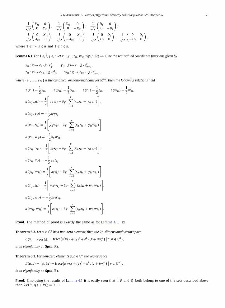
and for this we have the standard orthonormal basis consisting of the following elements
S. Gudmundsson, A. Sakovich / Differential Geometry and its Applications 27 (2009) 47–63 53
1√2
(Yrs 00 Yrs
),
1√2
(Xrs 00 −Xrs
),
1√2
(Dt 00 −Dt
),
1√2
(0 Xrs
Xrs 0
),
1√2
(0 Xrs
−Xrs 0
),
1√2
(0 Dt
Dt 0
),
1√2
(0 Dt
−Dt 0
),
where 1 � r < s � n and 1 � t � n.
Lemma 6.1. For 1 � i, j � n let xi j, yij, zi j, wij : Sp(n,R) → C be the real valued coordinate functions given by
xij : g → ei · g · etj, yij : g → ei · g · et
n+ j,
zi j : g → en+i · g · etj, wij : g → en+i · g · et
n+ j,
where {e1, . . . , e2n} is the canonical orthonormal basis for R2n. Then the following relations hold
τ (xij) = 1
2xij, τ (yij) = 1
2yij, τ (zi j) = 1
2zi j, τ (wij) = 1
2wij,
κ(xij, xkl) = 1
2
[yil ykj + δ jl ·
n∑t=1
(xit xkt + yit ykt)
],
κ(xij, ykl) = −1
2xil ykj,
κ(xij, zkl) = 1
2
[yil wkj + δ jl ·
n∑t=1
(xit zkt + yit wkt)
],
κ(xij, wkl) = −1
2xil wkj,
κ(yij, ykl) = 1
2
[xilxkj + δ jl ·
n∑t=1
(xit xkt + yit ykt)
],
κ(yij, zkl) = −1
2yil zkj,
κ(yij, wkl) = 1
2
[xil zkj + δ jl ·
n∑t=1
(xit zkt + yit wkt)
],
κ(zi j, zkl) = 1
2
[wil wkj + δ jl ·
n∑t=1
(zit zkt + wit wkt)
],
κ(zi j, wkl) = −1
2zil wkj,
κ(wij, wkl) = 1
2
[zil zkj + δ jl ·
n∑t=1
(zit zkt + wit wkt)
].
Proof. The method of proof is exactly the same as for Lemma 4.1. �Theorem 6.2. Let v ∈ C
n be a non-zero element, then the 2n-dimensional vector space
E (v) = {φab(g) = trace
(at v(x + iy)t + bt v(z + iw)t) ∣∣ a,b ∈ C
n},
is an eigenfamily on Sp(n,R).
Theorem 6.3. For non-zero elements a,b ∈ Cn the vector space
E (a,b) = {φv(g) = trace
(at v(x + iy)t + bt v(z + iw)t) ∣∣ v ∈ C
n},
is an eigenfamily on Sp(n,R).
Proof. Employing the results of Lemma 6.1 it is easily seen that if P and Q both belong to one of the sets described abovethen 2κ(P , Q ) + P Q = 0. �

54 S. Gudmundsson, A. Sakovich / Differential Geometry and its Applications 27 (2009) 47–63
7. Bi-eigenfamilies
The notion of an eigenfamily has in earlier sections turned out to be useful for the construction of harmonic morphismsfrom the Riemannian non-compact semisimple Lie groups SLn(R), SU∗(2n) and Sp(n,R). In order to solve the problem inthe cases of
SO∗(2n), SO(p,q), SU(p,q) and Sp(p,q)
we now generalize to the notion of a bi-eigenfamily.
Definition 7.1. Let (M, g) be a semi-Riemannian manifold and
E1 = {φi : M → C | i ∈ I1}, E2 = {ψi : M → C | i ∈ I2}be two non-empty eigenfamilies on M , i.e. there exist complex numbers λ1, μ1, λ2, μ2 such that
τ (φ1) = λ1φ1, κ(φ1, φ2) = μ1φ1φ2,
τ (ψ1) = λ2ψ1, κ(ψ1,ψ2) = μ2ψ1ψ2
for all φ1, φ2 ∈ E1 and ψ1,ψ2 ∈ E2. The union
B = E1 ∪ E2
is said to be a bi-eigenfamily on M if there exists a complex number μ such that
κ(φ,ψ) = μφψ
for all φ ∈ E1 and ψ ∈ E2.
Definition 7.2. Let m,n,d1,d2 be non-negative integers. Then a polynomial map P : Cm × C
n → C is said to be bi-homo-geneous of bi-degree d = (d1,d2) if for all λ,μ ∈ C
P (λz,μw) = λd1μd2 P (z, w).
The following result generalizes that of Theorem 2.5 and shows that bi-eigenfamilies are useful ingredients for theconstruction of harmonic morphisms.
Theorem 7.3. Let (M, g) be a semi-Riemannian manifold and B = E1 ∪ E2 be a finite bi-eigenfamily on M where
E1 = {φ1, . . . , φm} and E2 = {ψ1, . . . ,ψn}.If P , Q : C
m × Cn → C are linearly independent bi-homogeneous polynomials of the same bi-degree then the quotient
P (φ1, . . . , φm,ψ1, . . . ,ψn)
Q (φ1, . . . , φm,ψ1, . . . ,ψn)
is a non-constant harmonic morphism on the open and dense subset{p ∈ M
∣∣ Q(φ1(p), . . . , φm(p),ψ1(p), . . . ,ψn(p)
) �= 0}.
Proof. A proof of Theorem 7.3 can be found in Appendix A. �8. The Riemannian Lie group SO∗(2n)
In this section we construct eigenfamilies and bi-eigenfamilies of complex-valued functions on the non-compactsemisimple Lie group
SO∗(2n) = {q ∈ SU(n,n)
∣∣ q · Inn · Jn · qt = Inn · Jn},
where
U(n,n) = {z ∈ GL2n(C)
∣∣ z · In,n · z∗ = In,n}
and
Inn =(−In 0
0 I
), Jn =
(0 In
−I 0
).
n n

S. Gudmundsson, A. Sakovich / Differential Geometry and its Applications 27 (2009) 47–63 55
The Lie algebra so∗(2n) of SO∗(2n) is given by
so∗(2n) ={(
Z W−W̄ Z̄
)∈ C
2n×2n∣∣∣ Z + Z∗ = 0 and W + W t = 0
}
and for this we have the standard orthonormal basis consisting of the following matrices
1√2
(Yrs 00 Yrs
),
1√2
(i Xrs 0
0 −i Xrs
),
1√2
(iDt 00 −iDt
),
1√2
(0 Yrs
−Yrs 0
),
1√2
(0 iYrs
iYrs 0
),
where 1 � r < s � n and 1 � t � n.
Lemma 8.1. For 1 � i, j � n let zi j, wij : SO∗(2n) → C be the complex-valued coordinate functions given by
zij : q → ei · q · etj, wij : q → ei · q · et
n+ j,
where {e1, . . . , e2n} is the canonical orthonormal basis for C2n. Then the following relations hold
τ (zi j) = −1
2zi j, τ (wij) = −1
2wij,
κ(zi j, zkl) = −1
2zil zkj, κ(wij, wkl) = −1
2wil wkj,
κ(zi j, wkl) = 1
2
[zkj wil + δ jl ·
n∑t=1
(zit wkt − wit zkt)
].
Proof. The method of proof is exactly the same as for Lemma 4.1. �Theorem 8.2. Let v be a non-zero element of C
n. Then the vector spaces
E1(v) = {φa : SO∗(2n) → C
∣∣ φa(z + jw) = trace(vtazt), a ∈ Cn}
and
E2(v) = {ψc : SO∗(2n) → C
∣∣ ψc(z + jw) = trace(vtcwt), c ∈ Cn}
are eigenfamilies on SO∗(2n) and their union
B = E1(v) ∪ E2(v)
is a bi-eigenfamily.
Proof. If φa, φb ∈ E1(v) and ψc,ψd ∈ E2(v) then it is an immediate consequence of Lemma 8.1 that
τ (φa) = −1
2φa, τ (ψc) = −1
2ψc,
κ(φa, φb) = −1
2φaφb, κ(φb,ψc) = 1
2φbψc, κ(ψc,ψd) = −1
2ψcψd.
This proves the statement of Theorem 8.2. �Theorem 8.3. Let a be a non-zero element of C
n. Then the vector spaces
E1(a) = {φu : SO∗(2n) → C
∣∣ φu(z + jw) = trace(utazt), u ∈ Cn}
and
E2(a) = {ψv : SO∗(2n) → C
∣∣ ψv(z + jw) = trace(vtawt), v ∈ Cn}
are eigenfamilies on SO∗(2n).

56 S. Gudmundsson, A. Sakovich / Differential Geometry and its Applications 27 (2009) 47–63
9. Notation
In this section we introduce the necessary notation for dealing with the important non-compact cases SO(p,q), SU(p,q)
and Sp(p,q). Further we state a few matrix identities useful for those readers interested in the details of our calculations.For a positive integer n let p,q be non-negative integers such that n = p + q. Further let the index sets Δ1,Δ2,Λ1,Λ2
be defined by
Δ1 = {1, . . . , p}, Δ2 = {p + 1, . . . ,n},Λ1 = {
(r, s)∣∣ 1 � r < s � p or p + 1 � r < s � n
},
Λ2 = {(r, s)
∣∣ 1 � r � p and p + 1 � s � n}
and the matrices I pq, Jn by
I pq =(−I p 0
0 Iq
)and Jn =
(0 In
−In 0
).
With the above notation we have the following easily verified matrix identities
∑(r,s)∈Λ1
X2rs −
∑(r,s)∈Λ2
X2rs = −1
2
(In + (p − q)I pq
),
∑(r,s)∈Λ1
Y 2rs −
∑(r,s)∈Λ2
Y 2rs = 1
2
(In + (p − q)I pq
),
∑(r,s)∈Λ1
Xrs E jl Xtrs −
∑(r,s)∈Λ2
Xrs E jl Xtrs = 1
2
((−1)χ( j)+χ(l)+δ jl Elj + δ jl(−1)χ( j) I pq
),
∑(r,s)∈Λ1
Yrs E jlYtrs −
∑(r,s)∈Λ2
Yrs E jlYtrs = 1
2
((−1)χ( j)+χ(l)+1 Elj + δ jl(−1)χ( j) I pq
),
∑(r,s)∈Λ1
Xrs E jl Xtrs +
∑(r,s)∈Λ2
Yrs E jlYtrs +
n∑t=1
Dt E jl Dtt = 1
2
((−1)χ( j)+χ(l)+1 Elj + δ jl(−1)χ( j) In
).
Here χ : Z → {0,1} is the characteristic function for the set Δ1 given by
χ(i) ={
1, i ∈ Δ1,
0, i /∈ Δ1.
In the sequel we shall use the notation
Cp1 = {
(z, w) ∈ Cp × C
q∣∣ w = 0
}, C
q2 = {
(z, w) ∈ Cp × C
q∣∣ z = 0
}.
10. The Riemannian Lie group SU(p,q)
In this section we construct eigenfamilies on the non-compact Lie group U(p,q). These can be used to construct a varietyof local harmonic morphisms on the semisimple
SU(p,q) = {z ∈ SLp+q(C)
∣∣ z · I p,q · z∗ = I p,q}.
The Lie group U(p,q) is the non-compact subgroup of GLn(C) given by
U(p,q) = {z ∈ GLp+q(C)
∣∣ z · I p,q · z∗ = I p,q}.
The circle group S1 = {w ∈ C | |w| = 1} acts on U(p,q) by multiplication (w, z) → wz and the orbit space of this action isthe group SU(p,q). The Lie algebra u(p,q) of U(p,q) is given by
u(p,q) ={(
Z MM∗ W
)∈ glp+q(C)
∣∣∣ Z + Zt = 0 and W + W t = 0
}
with the canonical orthonormal basis{i Xrs, Yrs
∣∣ (r, s) ∈ Λ1} ∪ {
Xrs, iYrs∣∣ (r, s) ∈ Λ2
} ∪ {iDt∣∣ t = 1, . . . ,n}.
Lemma 10.1. For 1 � k, l � n let zkl : U(p,q) → C be the complex valued coordinate functions given by
zkl : z → ek · z · et,
l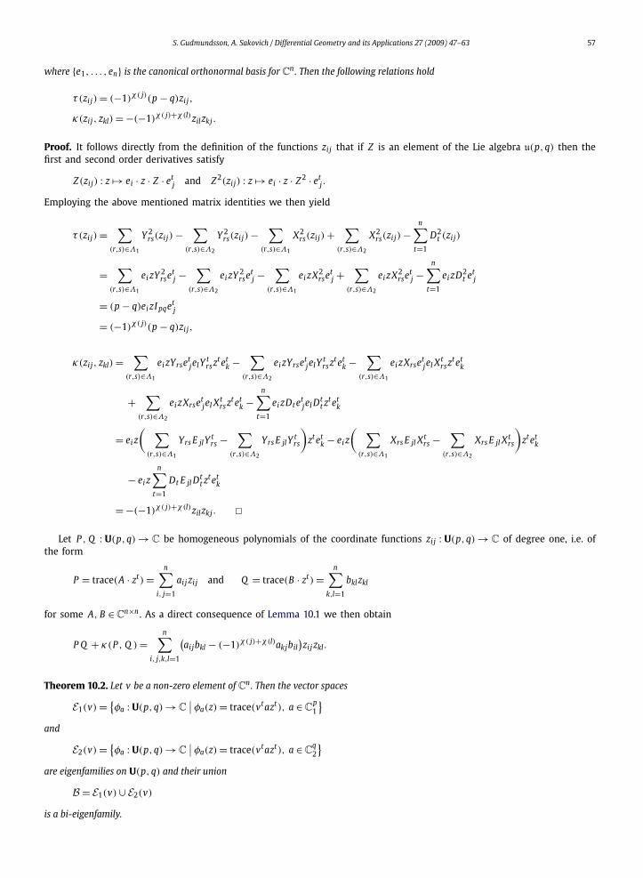
S. Gudmundsson, A. Sakovich / Differential Geometry and its Applications 27 (2009) 47–63 57
where {e1, . . . , en} is the canonical orthonormal basis for Cn. Then the following relations hold
τ (zi j) = (−1)χ( j)(p − q)zi j,
κ(zi j, zkl) = −(−1)χ( j)+χ(l)zil zkj .
Proof. It follows directly from the definition of the functions zi j that if Z is an element of the Lie algebra u(p,q) then thefirst and second order derivatives satisfy
Z(zi j) : z → ei · z · Z · etj and Z 2(zi j) : z → ei · z · Z 2 · et
j .
Employing the above mentioned matrix identities we then yield
τ (zi j) =∑
(r,s)∈Λ1
Y 2rs(zi j) −
∑(r,s)∈Λ2
Y 2rs(zi j) −
∑(r,s)∈Λ1
X2rs(zi j) +
∑(r,s)∈Λ2
X2rs(zi j) −
n∑t=1
D2t (zi j)
=∑
(r,s)∈Λ1
ei zY 2rset
j −∑
(r,s)∈Λ2
ei zY 2rset
j −∑
(r,s)∈Λ1
ei zX2rset
j +∑
(r,s)∈Λ2
ei zX2rset
j −n∑
t=1
ei zD2t et
j
= (p − q)ei zI pqetj
= (−1)χ( j)(p − q)zi j,
κ(zi j, zkl) =∑
(r,s)∈Λ1
ei zYrsetjelY
trsztet
k −∑
(r,s)∈Λ2
ei zYrsetjelY
trsztet
k −∑
(r,s)∈Λ1
ei zXrsetjel Xt
rsztetk
+∑
(r,s)∈Λ2
ei zXrsetjel Xt
rsztetk −
n∑t=1
ei zDtetjel D
tt ztet
k
= ei z
( ∑(r,s)∈Λ1
Yrs E jlYtrs −
∑(r,s)∈Λ2
Yrs E jlYtrs
)ztet
k − ei z
( ∑(r,s)∈Λ1
Xrs E jl Xtrs −
∑(r,s)∈Λ2
Xrs E jl Xtrs
)ztet
k
− ei zn∑
t=1
Dt E jl Dtt ztet
k
= −(−1)χ( j)+χ(l)zil zkj . �Let P , Q : U(p,q) → C be homogeneous polynomials of the coordinate functions zi j : U(p,q) → C of degree one, i.e. of
the form
P = trace(A · zt) =n∑
i, j=1
aij zi j and Q = trace(B · zt) =n∑
k,l=1
bkl zkl
for some A, B ∈ Cn×n . As a direct consequence of Lemma 10.1 we then obtain
P Q + κ(P , Q ) =n∑
i, j,k,l=1
(aijbkl − (−1)χ( j)+χ(l)akjbil
)zi j zkl.
Theorem 10.2. Let v be a non-zero element of Cn. Then the vector spaces
E1(v) = {φa : U(p,q) → C
∣∣ φa(z) = trace(vtazt), a ∈ Cp1
}and
E2(v) = {φa : U(p,q) → C
∣∣ φa(z) = trace(vtazt), a ∈ Cq2
}are eigenfamilies on U(p,q) and their union
B = E1(v) ∪ E2(v)
is a bi-eigenfamily.

58 S. Gudmundsson, A. Sakovich / Differential Geometry and its Applications 27 (2009) 47–63
Proof. Assume that a,b ∈ Cp1 and define A = vta and B = vtb. By construction any two columns of the matrices A and B
are linearly dependent. This means that for all 1 � i, j,k, l � n
det
(aij bilakj bkl
)= (aijbkl − akjbil) = 0
so P 2 + κ(P , P ) = 0, P Q + κ(P , Q ) = 0 and Q 2 + κ(Q , Q ) = 0. The fact that E1(v) is an eigenfamily is now a directconsequence of Lemma 10.1. A similar argument shows that E2(v) is also an eigenfamily. Note that κ(P , Q ) = P Q for anyP ∈ E1(v), Q ∈ E2(v). This shows that B is a bi-eigenfamily on U(p,q). �Theorem 10.3. Let u, v be two non-zero elements of C
p1 and C
q2 , respectively. Then the sets
E1(u) = {φa : U(p,q) → C
∣∣ φa(z) = trace(at uzt), a ∈ Cn}
,
E2(v) = {φa : U(p,q) → C
∣∣ φa(z) = trace(at vzt), a ∈ Cn}
are eigenfamilies on U(p,q).
Proof. The argument is similar to that used to prove the first part of Theorem 10.2. �It should be noted that the local harmonic morphisms on U(p,q) that we obtain by applying Theorem 7.3 are invariant
under the circle action and hence induce local harmonic morphisms on the semisimple Lie group SU(p,q).
11. The Riemannian Lie group SO(p,q)
In this section we construct eigenfamilies on the non-compact semisimple Lie group
SO(p,q) = {x ∈ SLp+q(R)
∣∣ x · I p,q · xt = I p,q}.
The Lie algebra so(p,q) of SO(p,q) is given by
so(p,q) ={(
A MMt B
)∈ slp+q(R)
∣∣∣ A + At = 0 and B + Bt = 0
}.
For this we have the canonical orthonormal basis{Yrs
∣∣ (r, s) ∈ Λ1} ∪ {
Xrs∣∣ (r, s) ∈ Λ2
}.
Lemma 11.1. For 1 � i, j � n let xi j : SO(p,q) → R be the real valued coordinate functions given by
xij : x → ei · x · etj,
where {e1, . . . , en} is the canonical orthonormal basis for Rn. Then the following relations hold
τ (xij) = 1
2
(1 + (−1)χ( j)(p − q)
)xij,
κ(xij, xkl) = 1
2
((−1)χ( j)+χ(l)+1xilxkj − δ jl(−1)χ( j)
[ ∑t∈Δ1
xit xkt −∑t∈Δ2
xit xkt
]).
Proof. The proof is similar to that of Lemma 10.1. �Let P , Q : SO(p,q) → C be homogeneous polynomials of the coordinate functions xij : SO(p,q) → C of degree one, i.e. of
the form
P = trace(A · xt) =n∑
i, j=1
aij xi j and Q = trace(B · xt) =n∑
k,l=1
bklxkl
for some A, B ∈ Cn×n . As a direct consequence of Lemma 11.1 we then obtain
P Q + 2κ(P , Q ) =n∑
i, j,k,l=1
aijbklxi j xkl + 2n∑
i, j,k,l=1
aijbklκ(xij, xkl)
=n∑
aijbklxi j xkl − (−1)χ( j)+χ(l)n∑
aijbklxilxkj
i, j,k,l=1 i, j,k,l=1

S. Gudmundsson, A. Sakovich / Differential Geometry and its Applications 27 (2009) 47–63 59
− δ jl(−1)χ( j)n∑
i, j,k=1
aijbkj
[ p∑t=1
xit xkt −p+q∑
t=p+1
xit xkt
]
=n∑
i, j,k,l=1
(aijbkl − (−1)χ( j)+χ(l)akjbil
)xij xkl − δ jl(−1)χ( j)
n∑i, j,k=1
aijbkj
[ p∑t=1
xit xkt −p+q∑
t=p+1
xit xkt
].
Comparing coefficients in the case when the integer χ( j) + χ(l) is even we see that P Q + 2κ(P , Q ) = 0 if for all1 � i,k � n
n∑j=1
aijbkj = 0
and
det
(aij bilakj bkl
)= (aijbkl − akjbil) = 0,
for all 1 � i, j,k, l � n.
Theorem 11.2. Let u be a non-zero element of Cn and V 1 , V 2 be maximal isotropic subspaces of C
p1 and C
q2 , respectively. Then the
vector spaces
EV 1 (u) = {φa : SO(p,q) → C
∣∣ φa(x) = trace(utaxt), a ∈ V 1}
and
EV 2 (u) = {φa : SO(p,q) → C
∣∣ φa(x) = trace(utaxt), a ∈ V 2}
are eigenfamilies on SO(p,q) and their union
B = EV 1 (u) ∪ EV 2 (u)
is a bi-eigenfamily.
Proof. Assume that a,b ∈ V 1 and define A = uta and B = utb. By construction any two columns of the matrices A and Bare linearly dependent. This means that for all 1 � i, j,k, l � n
det
(aij bilakj bkl
)= (aijbkl − akjbil) = 0.
Furthermore we have
P Q + 2κ(P , Q ) =n∑
j=1
aijbkj = uiuk(a,b) = 0.
Hence P 2 + 2κ(P , P ) = 0, P Q + 2κ(P , Q ) = 0, Q 2 + 2κ(Q , Q ) = 0. It follows directly from Lemma 11.1 that EV 1 (u) is aneigenfamily. A similar argument shows that EV 2 (u) is also an eigenfamily on SO(p,q). It is easy to see that 2κ(P , Q )− P Q =0 for any P ∈ EV 1 (u), Q ∈ EV 2 (u). This shows that B is a bi-eigenfamily on SO(p,q). �Theorem 11.3. Let u ∈ C
p1 and v ∈ C
q2 be two non-zero isotropic elements of C
n, i.e. (u, u) = (v, v) = 0. Then the sets
E1(u) = {φa : SO(p,q) → C
∣∣ φa(x) = trace(at uxt), a ∈ Cn}
and
E2(v) = {φa : SO(p,q) → C
∣∣ φa(x) = trace(at vxt), a ∈ Cn}
are eigenfamilies on SO(p,q).
Proof. The argument is similar to that used to prove the first part of Theorem 11.2. �
60 S. Gudmundsson, A. Sakovich / Differential Geometry and its Applications 27 (2009) 47–63
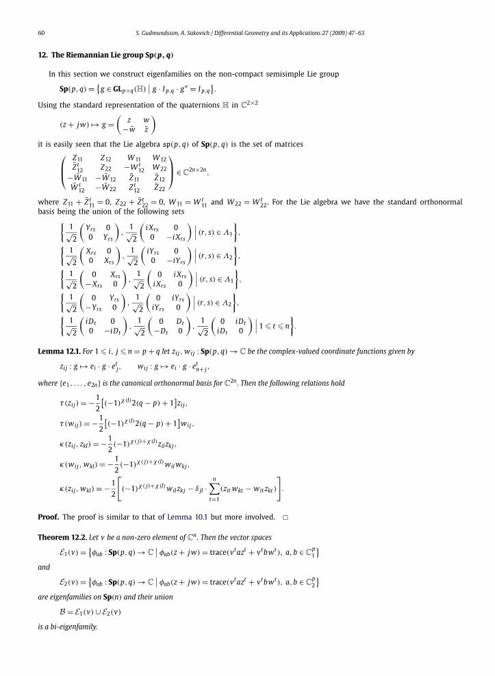
12. The Riemannian Lie group Sp(p,q)
In this section we construct eigenfamilies on the non-compact semisimple Lie group
Sp(p,q) = {g ∈ GLp+q(H)
∣∣ g · I p,q · g∗ = I p,q}.
Using the standard representation of the quaternions H in C2×2
(z + jw) → g =(
z w−w̄ z̄
)
it is easily seen that the Lie algebra sp(p,q) of Sp(p,q) is the set of matrices⎛⎜⎝
Z11 Z12 W11 W12Z̄ t
12 Z22 −W t12 W22
−W̄11 −W̄12 Z̄11 Z̄12W̄ t
12 −W̄22 Zt12 Z̄22
⎞⎟⎠ ∈ C
2n×2n,
where Z11 + Z̄ t11 = 0, Z22 + Z̄ t
22 = 0, W11 = W t11 and W22 = W t
22. For the Lie algebra we have the standard orthonormalbasis being the union of the following sets{
1√2
(Yrs 00 Yrs
),
1√2
(i Xrs 0
0 −i Xrs
) ∣∣∣ (r, s) ∈ Λ1
},
{1√2
(Xrs 00 Xrs
),
1√2
(iYrs 0
0 −iYrs
) ∣∣∣ (r, s) ∈ Λ2
},
{1√2
(0 Xrs
−Xrs 0
),
1√2
(0 i Xrs
i Xrs 0
) ∣∣∣ (r, s) ∈ Λ1
},
{1√2
(0 Yrs
−Yrs 0
),
1√2
(0 iYrs
iYrs 0
) ∣∣∣ (r, s) ∈ Λ2
},
{1√2
(iDt 00 −iDt
),
1√2
(0 Dt
−Dt 0
),
1√2
(0 iDt
iDt 0
) ∣∣∣ 1 � t � n
}.
Lemma 12.1. For 1 � i, j � n = p + q let zi j, wij : Sp(p,q) → C be the complex-valued coordinate functions given by
zij : g → ei · g · etj, wij : g → ei · g · et
n+ j,
where {e1, . . . , e2n} is the canonical orthonormal basis for C2n. Then the following relations hold
τ (zi j) = −1
2
[(−1)χ(l)2(q − p) + 1
]zi j,
τ (wij) = −1
2
[(−1)χ(l)2(q − p) + 1
]wij,
κ(zi j, zkl) = −1
2(−1)χ( j)+χ(l)zil zkj,
κ(wij, wkl) = −1
2(−1)χ( j)+χ(l) wil wkj,
κ(zi j, wkl) = −1
2
[(−1)χ( j)+χ(l) wil zkj − δ jl ·
n∑t=1
(zit wkt − wit zkt)
].
Proof. The proof is similar to that of Lemma 10.1 but more involved. �Theorem 12.2. Let v be a non-zero element of C
n. Then the vector spaces
E1(v) = {φab : Sp(p,q) → C
∣∣ φab(z + jw) = trace(vtazt + vtbwt), a,b ∈ Cp1
}and
E2(v) = {φab : Sp(p,q) → C
∣∣ φab(z + jw) = trace(vtazt + vtbwt), a,b ∈ Cp2
}are eigenfamilies on Sp(n) and their union
B = E1(v) ∪ E2(v)
is a bi-eigenfamily.

S. Gudmundsson, A. Sakovich / Differential Geometry and its Applications 27 (2009) 47–63 61
Proof. Let a,b, c,d be arbitrary elements of Cp1 and define the complex-valued functions P , Q : Sp(p,q) → C by
P = trace(vtazt + vtbwt) and Q = trace(vtczt + vtdwt).
Then a simple calculation shows that
P Q + 2κ(P , Q ) = [(a,d) − (b, c)
] n∑i,k,t=1
vi vk(zit wkt − wit zkt) = 0.
Automatically we also get P 2 + 2κ(P , P ) = 0 and Q 2 + 2κ(Q , Q ) = 0. It now follows directly from Lemma 11.1 that E1(v) isan eigenfamily. A similar argument shows that E2(v) is an eigenfamily on Sp(p,q). It is easy to see that 2κ(P , Q )− P Q = 0for any P ∈ E1(v), Q ∈ E2(v). This shows that B is a bi-eigenfamily on Sp(p,q). �13. The duality
In this section we show how a real analytic bi-eigenfamily B on a Riemannian non-compact semisimple Lie group Ggives rise to a real-analytic bi-eigenfamily B∗ on its semi-Riemannian compact dual U and vice versa. The method of proofis borrowed from a related duality principle for harmonic morphisms from Riemannian symmetric spaces, see [8].
Let W be an open subset of a non-compact semisimple Lie group G equipped with its standard Riemannian metric andφ : W → C be a real analytic map. Let GC denote the complexification of the Lie group G . Then φ extends uniquely to aholomorphic map φC : W C → C from some open subset W C of GC . By restricting this map to U ∩ W C we obtain a realanalytic map φ∗ : W ∗ → C from some open subset W ∗ of U .
Theorem 13.1. Let E be a family of maps φ : W → C and E ∗ be the dual family consisting of the maps φ∗ : W ∗ → C constructed asabove. Then E ∗ is an eigenfamily if and only if E is an eigenfamily.
Proof. Let g = k + p be a Cartan decomposition of the Lie algebra of G where k is the Lie algebra of a maximal compactsubgroup K . Furthermore let the left-invariant vector fields X1, . . . , Xn ∈ p form a global orthonormal frame for the distri-bution generated by p and similarly Y1, . . . , Ym ∈ k form a global orthonormal frame for the distribution generated by k. Weshall now assume that φ and ψ are elements of the eigenfamily E on the Riemannian W , i.e.
τ (φ) =m∑
k=1
Y 2k (φ) +
n∑k=1
X2k (φ) = λ · φ,
κ(φ,ψ) =m∑
k=1
Yk(φ)Yk(ψ) +n∑
k=1
Xk(φ)Xk(ψ) = μ · φ · ψ.
By construction and by the unique continuation property of real analytic functions the extension φC of φ satisfies the sameequations.
The Lie algebra of U has the decomposition u = k + ip and the left-invariant vector fields i X1, . . . , i Xn ∈ ip form a globalorthonormal frame for the distribution generated by ip. Then
τ (φ∗) = −m∑
k=1
Y 2k (φ∗) +
n∑k=1
(i Xk)2(φ∗) = −λ · φ∗,
κ(φ∗, φ∗) = −m∑
k=1
Yk(φ∗)Yk(ψ
∗) +n∑
k=1
(i Xk)(φ∗)(i Xk)(ψ
∗) = −μ · φ∗ · ψ∗.
This shows that E ∗ is an eigenfamily. The converse is similar. �Theorem 13.2. Let B be a family of maps φ : W → C and B∗ be the dual family consisting of the maps φ∗ : W ∗ → C constructed asabove. Then B∗ is a bi-eigenfamily if and only if B is a bi-eigenfamily.
Proof. The argument is similar to that used for Theorem 13.1. �14. The semi-Riemannian Lie group GLn(CCC)
Let h be the standard left-invariant semi-Riemannian metric on the general linear group GLn(C) induced by the semi-Euclidean scalar product on the Lie algebra gln(C) given by
h(Z , W ) = � e trace Z W .
62 S. Gudmundsson, A. Sakovich / Differential Geometry and its Applications 27 (2009) 47–63
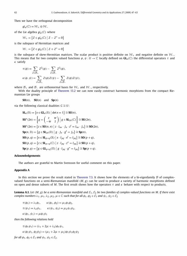
Then we have the orthogonal decomposition
gln(C) = W+ ⊕ W−of the Lie algebra gln(C) where
W+ = {Z ∈ gln(C)
∣∣ Z − Z∗ = 0}
is the subspace of Hermitian matrices and
W− = {Z ∈ gln(C)
∣∣ Z + Z∗ = 0}
is the subspace of skew-Hermitian matrices. The scalar product is positive definite on W+ and negative definite on W− .This means that for two complex valued functions φ,ψ : U → C locally defined on GLn(C) the differential operators τ andκ satisfy
τ (φ) =∑
Z∈B+Z 2(φ) −
∑Z∈B−
Z 2(φ),
κ(φ,ψ) =∑
Z∈B+Z(φ)Z(ψ) −
∑Z∈B−
Z(φ)Z(ψ),
where B+ and B− are orthonormal bases for W+ and W− , respectively.With the duality principle of Theorem 13.2 we can now easily construct harmonic morphisms from the compact Rie-
mannian Lie groups
SO(n), SU(n) and Sp(n)
via the following classical dualities G ∼= U :
SLn(R) = {x ∈ GLn(R)
∣∣ det x = 1} ∼= SU(n),
SU∗(2n) ={
g =(
z w−w̄ z̄
) ∣∣∣ g ∈ SL2n(C)
}∼= SU(2n),
SO∗(2n) = {z ∈ SU(n,n)
∣∣ z · Inn · Jn · zt = Inn · Jn} ∼= SO(2n),
Sp(n,R) = {g ∈ SL2n(R)
∣∣ g · Jn · gt = Jn} ∼= Sp(n),
SO(p,q) = {x ∈ SLp+q(R)
∣∣ x · I pq · xt = I pq} ∼= SO(p + q),
SU(p,q) = {z ∈ SLp+q(C)
∣∣ z · I pq · z∗ = I pq} ∼= SU(p + q),
Sp(p,q) = {g ∈ GLp+q(H)
∣∣ g · I pq · g∗ = I pq} ∼= Sp(p + q).
Acknowledgements
The authors are grateful to Martin Svensson for useful comment on this paper.
Appendix A
In this section we prove the result stated in Theorem 7.3. It shows how the elements of a bi-eigenfamily B of complex-valued functions on a semi-Riemannian manifold (M, g) can be used to produce a variety of harmonic morphisms definedon open and dense subsets of M . The first result shows how the operators τ and κ behave with respect to products.
Lemma A.1. Let (M, g) be a semi-Riemannian manifold and E1, E2 be two families of complex-valued functions on M. If there existcomplex numbers λ1,μ1, λ2,μ2,μ ∈ C such that for all φ1, φ2 ∈ E1 and ψ1,ψ2 ∈ E2
τ (φ1) = λ1φ1, κ(φ1, φ2) = μ1φ1φ2,
τ (ψ1) = λ2ψ1, κ(ψ1,ψ2) = μ2ψ1ψ2,
κ(φ1,ψ1) = μφ1ψ1
then the following relations hold
τ (φ1ψ1) = (λ1 + 2μ + λ2)φ1ψ1,
κ(φ1ψ1, φ2ψ2) = (μ1 + 2μ + μ2)φ1ψ1φ2ψ2
for all φ1, φ2 ∈ E1 and ψ1,ψ2 ∈ E2 .

S. Gudmundsson, A. Sakovich / Differential Geometry and its Applications 27 (2009) 47–63 63
Proof. The statement is an immediate consequence of the following basic facts concerning first and second order derivativesof products
X(φ1ψ1) = X(φ1)ψ1 + φ1 X(ψ1),
X2(φ1ψ1) = X2(φ1)ψ1 + 2X(φ1)X(ψ1) + φ1 X2(ψ1). �The following result shows how the operators τ and κ behave with respect to quotients.
Lemma A.2. Let (M, g) be a semi-Riemannian manifold and P , Q : M → C be two complex-valued functions on M. If there exists acomplex number λ ∈ C such that
τ (P ) = λP and τ (Q ) = λQ
then the quotient φ = P/Q is a harmonic morphism if and only if
Q 2κ(P , P ) = P Q κ(P , Q ) = P 2κ(Q , Q ).
Proof. For the first and second order derivatives of the quotient P/Q we have the following basic facts
X(φ) = X(P )Q − P X(Q )
Q 2,
X2(φ) = Q 2 X2(P ) − 2Q X(P )X(Q ) + 2P X(Q )X(Q ) − P Q X2(Q )
Q 3
leading to the following formulae for τ (φ) and κ(φ,φ)
Q 3τ (φ) = Q 2τ (P ) − 2Q κ(P , Q ) + 2Pκ(Q , Q ) − P Q τ (Q ),
Q 4κ(φ,φ) = Q 2κ(P , P ) − 2P Q κ(P , Q ) + P 2κ(Q , Q ).
The statement is a direct consequence of those relations. �Proof of Theorem 7.3. For the finite eigenfamilies E1 and E2 on M we define the infinite sequences
{E k1}∞k=1 and {E k
2}∞k=1
by induction
E 11 = E1, E k+1
1 = E k1 · E1 = {
φ · φ1∣∣ φ ∈ E k
1, φ1 ∈ E1},
E 12 = E2, E k+1
2 = E k2 · E2 = {
ψ · ψ1∣∣ ψ ∈ E k
2 , ψ1 ∈ E2}.
It then follows from the fact that
κ(φ,φ1) = kμ1φφ1
for all φ ∈ E k1 and φ1 ∈ E 1
1 and Lemma A.1 that each E k+11 is an eigenfamily on M . The same is of course true for each E k+1
2 .A simple calculation shows that for all Φ ∈ E k
1 , Ψ ∈ E l2
κ(Φ,Ψ ) = μ · k · l · Φ · Ψ.
With this at hand the statement of Theorem 7.3 is an immediate consequence of Lemma A.2. �References
[1] P. Baird, J. Eells, A conservation law for harmonic maps, in: Geometry Symposium Utrecht 1980, in: Lecture Notes in Mathematics, vol. 894, Springer,1981, pp. 1–25.
[2] P. Baird, J.C. Wood, Harmonic Morphisms Between Riemannian Manifolds, London Math. Soc. Monogr., vol. 29, Oxford Univ. Press, 2003.[3] B. Fuglede, Harmonic morphisms between Riemannian manifolds, Ann. Inst. Fourier 28 (1978) 107–144.[4] B. Fuglede, Harmonic morphisms between semi-Riemannian manifolds, Ann. Acad. Sci. Fennicae 21 (1996) 31–50.[5] S. Gudmundsson, The bibliography of harmonic morphisms, http://www.matematik.lu.se/matematiklu/personal/sigma/harmonic/bibliography.html.[6] S. Gudmundsson, On the existence of harmonic morphisms from symmetric spaces of rank one, Manuscripta Math. 93 (1997) 421–433.[7] S. Gudmundsson, A. Sakovich, Harmonic morphisms from the classical compact semisimple Lie groups, Ann. Global Anal. Geom. 33 (2008) 343–356.[8] S. Gudmundsson, M. Svensson, Harmonic morphisms from the Grassmannians and their non-compact duals, Ann. Global Anal. Geom. 30 (2006) 313–
333.[9] S. Gudmundsson, M. Svensson, On the existence of harmonic morphisms from certain symmetric spaces, J. Geom. Phys. 57 (2007) 353–366.
[10] T. Ishihara, A mapping of Riemannian manifolds which preserves harmonic functions, J. Math. Kyoto Univ. 19 (1979) 215–229.[11] A.W. Knapp, Lie Groups Beyond an Introduction, Birkhäuser, 2002.