harmonic decomposition of a vibroseis sweep … · harmonic decomposition of a vibroseis sweep ......

Harmonic decomposition of a Vibroseis sweep

CREWES Research Report — Volume 23 (2011) 1

HARMONIC DECOMPOSITION OF A VIBROSEIS SWEEP USING GABOR ANALYSIS

Christopher B. Harrison, Gary Margrave, Michael Lamoureux, Arthur Siewert, and Andrew Barrett

ABSTRACT In traditional Vibroseis surveys the harmonic frequencies generated by the vibrator are

seen as undesirable noise distortions. These distortions are attributed to various factors such as nonlinear coupling of the vibrator to the ground, nonlinear effects in the vibrator and inadequacy of the feedback system. These harmonic effects cause a correlation-ghost forerunner or a tail at both positive and negative correlation times if the harmonically distorted sweep is used as the correlation operator. Over the years techniques for bulk attenuation of these harmonic effects have been developed to enhance Vibroseis seismic imaging. An innovative approach, however, is proposed to decompose Vibroseis sweeps into their respective fundamental and harmonic components such that the harmonics and their higher frequencies can be used for seismic imaging or more accurate filter design. The decomposition is accomplished through the use of the Gabor transform to produce broad band estimates of the fundamental and harmonics of the Vibroseis sweep. The method is tested on both a synthetic sweep with time varying amplitude and phase, as well as field data.

INTRODUCTION Since its introduction in 1960, Vibroseis has become the preferred source for land

seismic where conditions allow. The source of the Vibroseis, or the sweep, is created by the excitation of the vibrator by a pilot signal which varies over a designed frequency range. For thin bed imaging it is desired that higher frequencies be preserved in the Vibroseis source. However, harmonics, and even sub-harmonics, are generated during the sweep excitation by nonlinear effects in the earth and the Vibroseis machinery itself.

Processing of Vibroseis data requires correlation of the raw data with a sweep to produce correlated records comparable to those from impulsive sources. Since the sweep also contains harmonics from nonlinear effects, the correlation process yields a non-zero phase Klauder wavelet. The results will either be a correlation-ghost forerunner or a tail at both positive and negative correlation times (Sheriff and Kim, 1970). Methods have been developed to remove the harmonic “distortions” to improve seismic imaging. Improvement to Vibroseis methods fall under two categories: 1) improvement of data quality or 2) enhance acquisition efficiency (Abd El-Aal 2011). Enhanced acquisition techniques such as simultaneous shooting, cascade sweeps, slip-sweeps and simultaneous slip-sweep have been designed to improve data quality (Gagaini 2010). Phase control systems have also been developed in modern vibrators to compensate for the phase shift. Ambient noise attenuation techniques are applied either in the acquisition phase or later on in processing.

An innovative approach to analyzing harmonic distortions is proposed here. Since the nonlinear harmonics have known time-frequency dependence, a least squares

Harrison et al.

2 CREWES Research Report — Volume 23 (2011)

minimization utilizing the Gabor spectra of individual components can accurately decompose a sweep into its fundamental and harmonics. These accurately reconstructed components can them be utilized for filter designs, or if the data is conditioned properly, the higher order harmonics can be used as higher frequency sources.

The nomenclature of harmonics tends to be confused between different literary sources. The “fundamental” component refers to the frequency range that the original pilot sweep was restricted to. In this paper we will use the first harmonic, H2, as twice the fundamental frequency. This is followed by the second harmonic, H3, and so forth. While it is possible to consider extremely high order harmonics, say H10 and higher, attenuation through the top layers of the earth and sampling rates limits the harmonic that are resolvable. As will be shown below, H7 appears to be the sufficiently high order harmonic that successfully contributes to the decomposition using the currently designed algorithm.

Survey Data The Vibroseis sweeps studied in this paper are from a 2D seismic survey generously

supplied by the sponsor company, Statoil. The survey was conducted in September of 2009 on a dirt road that had been iced down (water sprayed on the surface) in northern Alberta, Canada. Good coupling between the ground and vibrator was achieved on the firm ice pack of the road. Sweep parameters, which are critical to harmonic decomposition, are supplied in Table 1:

Weight 12500 lb Number of Vibes 1

Sweep Type 6 – 240 Hz non-linear Sweep Length 20000 ms Sample Rate 0.5 ms

Boost 0.09 dB/octave Table 1. Vibrator parameters

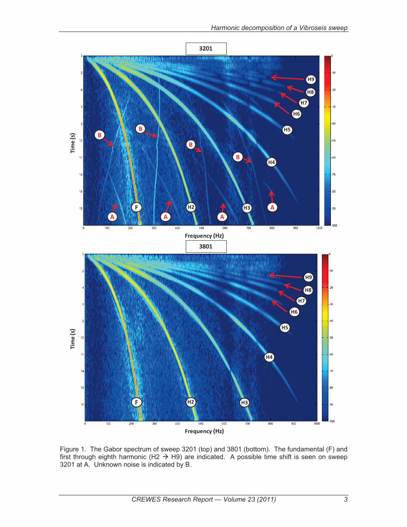
Two recorded sweeps from the baseplate were chosen from this survey for initial Gabor spectra observation. Figure 1 shows the Gabor spectrum of sweep 3201 and 3801. The bottom sweep, which will be the main focus of harmonic decomposition, is sweep 3801. Sweep 3801 was chosen due to its high single-to-noise ratio. The top sweep in Figure 1 is 3201 which shows some interesting noise on its Gabor spectra. Each sweep spectrum in Figure 1 shows the location of the fundamental, H2 through to H9.

Sweep 3201 shows a possible time shifted ghost highlighted by the "A" indicators on Figure 1. The noise highlighted by “B” indicators is presently unknown. These noise patterns are not unique to this sweep, but seen on other sweeps in the survey. This sweep, however, is only used for brief comparison and may be the subject for a future study. Sweep 3801, on the other hand, is a good example of a sweep with high single-to-noise (SN) ratio and good ground coupling. Due to this high SN ratio, sweep 3801 will be the field example focus for the remainder of harmonic decomposition.



Figure 1. The Gabor spectrum of sweep 3201 (top) and 3801 (bottom). The fundamental (F) and first through eighth harmonic (H2 � H9) are indicated. A possible time shift is seen on sweep 3201 at A. Unknown noise is indicated by B.

Frequency (Hz)

3801

3201

Tim

e (s

)

Frequency (Hz)

Tim

e (s

)

F H2 H3

H4

H5

H6

H7

H8

H9

F H2 H3

H4

H5

H6

H7

H8

H9

A A AA

BB

B

B

Harrison et al.


Figure 2 shows the uncorrelated shot record for sweep 3801. Traces 10, 40, 70, 80, 108, 120, 150 and 180 have been selected as the locations to investigate harmonic distortions. Figure 3 shows the Gabor spectrum for each traces noted in Figure 2. The fundamental, first (H2), second (H3) and third (H4) harmonics can clearly be seen in the near offsets. This near offset dependence suggests that utilization of any higher order harmonics, the first (H2) or second (H3), will be most effective at near offsets.

Figure 2. Shot record for sweep 3801. Traces 10, 40, 70, 80, 108 (110 was too noisy), 120,150 and 180 are noted for Gabor spectrum analysis.

Shot 3801

Trace Num.

Tim

e (s

)

10 40 70 80 108 120 150 180



Figure 3. Gabor spectrum of traces 10, 40, 70, 80, 108, 120, 150 and 180. Harmonics are stronger on near offset and almost negligible on far offset.

Trace - 10 Trace - 40




Harrison et al.


Composition of a Vibroseis Sweep The ability to attenuate noise from the Vibroseis signal is linked directly to the

improvement of seismic imaging. There are two types of noise that are inherent in Vibroseis seismic acquisition: environmental, which include wind, electric wires, traffic, etc and source-generated noise within the vibrator itself. To increase the signal-to-noise ratio (SN) operators and processors have developed techniques to increase source power through multiple shots, shot and CDP stacking, improved array design, phase loop corrections, and migration techniques.

Source-generated harmonics are mainly attributed to nonlinear mechanisms in the vibrators hydraulic system and baseplate-ground coupling due to low rigidity of the baseplate (Wei 2007; Wei 2011). Specific contributors to harmonic generation include, nonlinear forced vibrational response from mechanical electrical and hydraulic systems, stiffness and deformation of the baseplate, mechanical fault, timer-variance, frequency-dependence physical properties and structures of near source excitation, (Guan Yezhi 2009) are but a few.

These harmonics have traditionally been treated as noise to be attenuated. The harmonics have known frequency-dependence, however, and through proper data conditioning, each harmonic can be decomposed from the distorted signal. To begin the decomposition of the distorted sweep we assume an uncorrelated signal in the time domain as follows:

( ) ( )* ( ) * ( )ds dsp t t e t n t� �� (1)

where ( )ds t� is the distorted sweep (ds) with harmonics, ( )e t is the earth response, ( )n t is additive random noise, and * represents convolution. For simplicity in derivation the random noise term, * ( )ds n t� , will be neglected leaving

( ) ( )* ( )dsp t t e t�� . (2)

The sweep ( )ds t� is the sum of the fundamental ( 1� ) and all (n) harmonics

1 1 2 2 3 3

1( ) * ( ) * ( ) * ( ) * ( ) ... * ( ) ...

N

ds n n n nn

t t t t t t� � � � � � � � � � ��

� � � � � � �� (3)

where all n� are small time-independent convolutional (*) filters. In our model, the n� filters are dependent on the nature of the distortion mechanism (phase, amplitude, etc) as well as the rate of change in the instantaneous frequency (Li 1997). At present we assume the n� to be stationary (time-independent) but we will overcome that limitation with a reformulation in the Gabor domain. Substituting equation (3) into (2) results in:



1 1

2( ) ( * ( ) * ( ))* ( )

N

n nn

p t t t e t� � � ��

� �� (4)

which can be written as

1 1

2( ) * ( )* ( ) * ( )* ( )

N

n nn

p t t e t t e t� � � ��

� ��. (5)

Equation (5) is the uncorrelated trace without ambient noise. Traditional processing

would treat the term 2

* ( )* ( )N

n nn

t e t� �� collectively as noise to be attenuated from the

trace. However, expanding equation(5):

1 1 2 2 3 3( ) * ( )* ( ) * ( )* ( ) * ( )* ( ) * ( )* ( ) ...n np t t e t t e t t e t t e t� � � � � � � �� (6)

provides an equation for an uncorrelated signal in the time domain with specific values for the fundamental and n harmonics. Depending on depth and sample rate, there is only a finite number of harmonics that will be resolvable. As can be seen on Figure 3, high order harmonics will naturally be attenuated through the earth. H10 also appears to be the limit for resolvable harmonics on Figure 1 for the baseplate.

Equation (3) and (6) provides a base for four unique methods to solve for the coefficients. These solutions are the time stationary, frequency stationary, time-dependant Gabor solution and the frequency-dependant Gabor solution.

Time Stationary Solution

In this case we assume the n� degenerate from convolutional filters to simple scalar multipliers na . Solving for the coefficients in equation (3) with respect to time is the simplest and least accurate of the solutions provided in this paper. This time stationary method, however, does provide us with a base by which to gage all subsequent solutions. Using an objective function:

2

11

( ,..., )N

N ds nf a a � �� (7)

and taking the convenience 2N � , it follows that

2

1 2 1 1 2 2( , ) ( )dsi

f a a a a� � �� (8)

and

2 2 2 2 2

1 2 1 1 2 2 1 1 1 2 1 2 2 2( , ) 2 2 2ds ds dsi

f a a a a a a a a� � � � � � � � �� (9)

where minimization of 1a

Harrison et al.


1 1 1 1 2 2 1

1

0 2( )dsf a aa

� � � � � �� (10)

works out to

1 1 1 2 2 1 1dsa a� � � � � �� . (11)

Followed by the minimization with respect to 2a

2 1 1 2 2 2 2

2

0 2( )dsf a aa

� � � � � �� (12)

which comes to

1 1 2 2 2 2 2dsa a� � � � � �� . (13)

Combining equation (11) and equation (13) leads to

1 1 1 2 1 1

2 1 2 2 2 2

ds

ds

aa

� � � � � ��

�� .

(14)

Inverting (14) to acquire coefficients:

111 1 1 2 1

22 1 2 2 2

ds

ds

aa

� ��

�

� � �� . (15)

In the case of N harmonics equation (15) becomes:

11 11 1 1 2 1

1 2 2 2

1

......... ... ......... ... ... ... ...

... ...

N ds

n N N N ds N

a

a

� � � ��

� � � � � �

� � � � ��

� � � . (16)

Equation (16) provides the coefficients of the fundamental and N harmonics for the time stationary solution to equation (3).

Frequency Stationary Solution The next most accurate solution to the coefficients in equation (3) is the frequency

stationary method. This solution is slightly more accurate due to an added phase rotation being revealed. A Fourier transform is applied to equation (3) as follows:

1( ( )) ( * )

N

j ds j n nn

F t F� � ��

� � (17)

where the subscript j denotes frequency. This is then written as:



1 1 2 2 3 3ˆ ˆ ˆ ˆ... ...dsj j j j n njg g g g g� � � �� (18)

where ˆn� are the Fourier transforms of the n� , dsjg is ( ( ))j dsF t� and njg are ( ( ))j nF t� . In what follows, we assume that all ˆn� are constants (independent of frequency). Minimization of equation (18) via the objective function:

2

11

ˆ ˆ ˆ( ,..., )N

j Nj dsj nj njn

f g g� � ��

� ��. (19)

Again, for simplicity we limit ourselves to the fundamental and the first harmonic

2

1 2 1 1 2 2ˆ ˆ ˆ ˆ( , ) dsj j jj

f g g g� � � �� (20)

which becomes

1 2 1 1 2 2 1 1 2 2ˆ ˆ ˆ ˆ ˆ ˆ( , ) ( )( )dsj j j dsj j j

jf g g g g g g� � � � � ��

(21)

where the over bar indicates complex conjugation. To find the complex coefficients we minimize (21) similar to Appendix A. This then has the unique minimum

1

1 1 2 1 11

2 1 2 2 2 2

ˆˆ

j j j j dsj jj j j

j j j j dsj jj j j

g g g g g g

g g g g g g

��

� � � � �

� � � � ��

� �

� � �

� � � (22)

and in the case of N harmonics

1

1 1 2 1 11

1

1 2 2 2

1

...ˆ...... ... ......... ... ... ... ...

ˆ

... ...

j j j j Nj jdsj jj j j

j

j j j jj j

N dsj Njj Nj Nj Nj j

j j

g g g g g g g g

g g g g

g gg g g g

�

�

� � � � � � � � ��

� � � ��

�� . (23)

This solution to equation (3) is slightly more flexible than the time stationary case because it models a possible constant phase rotation for each harmonic. However, this solution is still not as general as the Gabor solutions discussed below.

Time and Frequency dependant Gabor Solution The Gabor transform is a nonstationary generalization of the Fourier transform

(Margrave 2004). Using the Gabor transform to solve equation (3) will provide us with estimates of the complex-valued, time-frequency function that we can call the spectrum of the fundamental, harmonics and input sweep.

Harrison et al.


A general case of harmonic decomposition of a distorted sweep using the Gabor transform is first derived. Applying the continuous Gabor transform to the distorted sweep as seen in equation (3) results in,

1( ) ( * )

N

ij ds ij n nn

G G� � ��

� �. (24)

Here we use subscript i for time and j for frequency. This can be manipulated to,

1 1 2 2 3 3( ) ( ) ( ) ( ) ( ) ( ) ( ) ... ( ) ( ) ...ij ds ij ij ij ij ij ij ij N ij NG G G G G G G G G� � � � � � � � �� . (25)

This equation uses the approximation ( * ) ( ) ( )ij n n ij n ij nG G G� � � �� which is justified in Margrave et al (2011). Then we define the Gabor coefficient as

ˆ( )ij n nijG � �� , (26)

followed by

( )ij ds dsijG h� � , (27)

and

( )ij n nijG h� � (28)

where equation (25) becomes

1 1 2 2 3 3ˆ ˆ ˆ ˆ... ...dsij ij ij ij ij ij ij nij nijh h h h h� � � �� . (29)

The subscript i is with respect to time and j is with respect to is frequency. To solve equation (29) for desired ˆnij� we propose two alternative methods. In one case ˆnij� are dependant only on i (i.e. time) or in the other case solution are dependant only on j (i.e. frequency), but not both. The first case with respect to i is the time dependant Gabor decomposition and the second case with respect to j is the frequency dependant Gabor decomposition.

For the time dependant Gabor decomposition we solve for each time i to find the best ˆnj� as follows. The objective function

2

11

ˆ ˆ ˆ( ,..., )N

ij Nij dsij nij nijn

f h h� � ��

� �� (30)

is used in case of all i (time) and the fundamental and first harmonic:



2

1 2 1 1 2 2ˆ ˆ ˆ ˆ( , )i i dsij i ij i ijj

f h h h� � � �� (31)

which expands to

� �1 2 1 1 2 2 1 1 2 2ˆ ˆ ˆ ˆ ˆ ˆ( , ) ( )( )i i dsij i ij i ij dsij i ij i ij

jf h h h h h h� � � � � ��

(32)

and minimization equation (32) to find the complex coefficients (Appendix A)

1

1 1 2 1 11

2 1 2 2 2 2

ˆˆ

ij ij ij ij dsij ijj j ji

i ij ij ij ij dsij ijj j j

h h h h h h

h h h h h h

��

� � � � �

� � � � ��

� �

� � �

� � �. (33)

In the case of N harmonics,

1

1 1 2 1 11

1

1 2 2 2

1

...ˆ...... ... ......... ... ... ... ...

ˆ

... ...

ij ij ij ij Nij ijdsij ijj j j

ji

ij ij ij ijj j

Ni dsij Nijij Nij Nij Nij j

j j

h h h h h h h h

h h h h

h hh h h h

�

�

� � � � � � � � ��

� � � ��

�� . (34)

Similarly, in the case of each frequency j equation (33) becomes

1

1 1 2 1 11

2 1 2 2 2 2

ˆˆ

ij ij ij ij dsij ijj i i i

j ij ij ij ij dsij iji i i

h h h h h h

h h h h h h

��

�

� � � ��

� � �

� � � (35)

In the case of each frequency j and N harmonics equation (35) becomes

1

1 1 2 1 11

1

1 2 2 2

1

...ˆ...... ... ......... ... ... ... ...

ˆ

... ...

ij ij ij ij Nij ijdsij iji i i

j i

ij ij ij iji i

Nj dsij Nijij Nij Nij Nij i

i i

h h h h h h h h

h h h h

h hh h h h

�

�

� � � � ��

� � � ��

�� (36)

The inversion as seen in both the time dependant Gabor decomposition in equation (34) and frequency dependant Gabor decomposition in equation (36) are both unstable. A stability factor is developed below.

Harrison et al.


Time and frequency dependant Gabor decomposition stability factor Both the time dependant Gabor decomposition and frequency dependant Gabor

decompositions in equations (34) and (36) are unstable with possible zeros or sufficiently small values to make inversion calculation unstable. Starting with the un-inverted time dependant Gabor decomposition of equation (33)

1 1 2 1 11

21 2 2 2 2

ˆˆ

ij ij ij ij dsij ijj j ji

iij ij ij ij dsij ijj j j

h h h h h h

h h h h h h

��

� � � �

��

� �

� � �

� � � (37)

where we assign

1 1 2 1

1 2 2 2

ij ij ij ijj j

jij ij ij ij

j j

h h h h

h h h h�

� �

� � ��

� �

� � (38)

resulting in

11

2 2

ˆˆ

dsij ijji

ji dsij ij

j

h h

h h

��

�

� �

� � ��

�

�

�. (39)

We propose the following to stabilize equation (39). Equation (39) is multiplied by T

j� to ensure j� is square and invertible. A stability function jMaxb� � is added only to the left side of Equation (39) to add non-zero real values into the diagonal of the square matrix T

j j� � as follows:

11

2 2

ˆˆ

dsij ijji T

jStab ji dsij ij

j

h h

h h

��

�

� �

� � ��

�

�

� (40)

where,

( )TjStab j j jMaxb� � � � ��

, (41)

and

max( )T

jMax j j� � ��. (42)

The expression b is a stability factor and is the unit matrix. Inverting (40) results in,



11 1

2 2

ˆ( )

ˆ

dsij ijji T T

j j jMax ji dsij ij

j

h hb

h h

��

��

� �

� � � ��

�

�

�

. (43)

The stability factor, b, is chosen through trial and error to best resolve the data. In the case of N harmonics with respect to i (time) equation (43) appears as

11

1

ˆ... ( ) ...ˆ

dsij ijji

T Tj j jMax j

Ni dsij Nijj

h h

b

h h

��

�

�

� � � ��

�

� (44)

where

1 1 1

1

...

... ... ...

...

ij ij Nij ijj j

j

ij Nij Nij Nijj j

h h h h

h h h h

�

� ��

� �

� �

.

(45)

In the case of N harmonics with respect for j (frequency):

11

1

ˆ... ( ) ...ˆ

dsij ijij

T Ti i iMax i

Nj dsij Niji

h h

b

h h

��

�

�

� ��

�

� (46)

where

1 1 1

1

...

... ... ...

...

ij ij Nij iji i

i

ij Nij Nij Niji i

h h h h

h h h h

�

� ��

� �

� �. (47)

These two final equations for the stabilized time dependant Gabor decomposition and

stabilized frequency dependant Gabor decompositions in equations (44) and (46), respectively, are the main focus for the remainder of this study. These two equations are considered more general than the time stationary or frequency stationary in equations

Harrison et al.


(16) and (23) respectively. As will be shown below, the frequency dependant Gabor decomposition appears to best decompose a desired sweep.

Sweep Design To find the coefficients in equations (44) and (46) we have to calculate fundamental

( 1� ) and all desired harmonic ( n� ). Calculating these sweeps requires the knowledge of how the original pilot sweep has been created. In the case of this study the pilot sweep equation was found in the Sercel VE464 Vibroseis user manual (Sercel 2010). The Sercel equation appears as follows:

1( ) log 1 ( 1)1log( )

Fe Fb tFi t FbT SegRa

SegRa

� ��

� � (48)

where

� SegRa = Sb/Se = 10

� Sb = Slope at the start of the log segment

(-Ra/10)

� Se = Slope at the end of the log segment

� Fb = Start frequency

� Fe = End Frequency

� T = Te – Tb = Basic signal length

� Ra represents the attenuation (in dB) within the signal spectrum.

Derivation of the sweep is non-trivial. The pilot sweep equations may be unique for the each Vibroseis and acquisition company. The algorithm utilized in this paper may fail if the pilot sweep of a different Vibroseis is used as an input. Sweep designs should be derived as needed. However, it is also proposed that knowledge of the original sweep equation is not necessary by using the time sequence of the pilot sweep with manipulations of the Fourier transform to compute all harmonics.

Algorithm: harmonicdecom As of November 2011, the algorithm for harmonic decomposition has been designed

to accept 12 input parameters with three output arguments. The algorithm will be available upon request to CREWES sponsors (though it is still in the testing phase) and will be available in the CREWES Matlab libraries in the future. This function is presently designed with the Sercel sweep as described above. Further sweep types will be added as needs arise. The function has the following arguments:

ControlSweep: The control sweep for decomposition



ControlTime: The time vector for the control sweep. Sample rate is taken from this input.

strf*: The starting frequency for the sweep.

endf*: The end frequency of the sweep

alpha : The boost in db/Hz.

taper*: Length of the cosine sweep taper in seconds.

This value has to match acquisition parameters

nharm: The components to be decomposed where 1 is the fundamental.

outflag*: The type of sweep, where 1 is displacement, 2 is velocity and 3 is acceleration.

haflwidth*: Gabor parameter for the half width of the Gaussian window.

tshift*: Gabor parameter for length of temporal shift

p*: Gabor parameter, exponent used in the analysis window

gdb: The number of decibels below 1 at which to truncate the Gaussian window.

stabfactor*: The stability factor.

SweepsOut: Array of time, decomposed fundamentals and harmonics with respect to time and frequency.

ComplexTimeScale: Array of scalars used to find each time dependant decomposition results

ComplexFreqScale: Array of scalars used to find each frequency dependant decomposition results

The parameters marked with an “*” are selected through trial and error for best results. While the frequency range of the sweep is known, results of harmonic decomposition are sensitive to initial choice of start and end frequency. The “alpha” parameter is extremely sensitive and requires the original value used during acquisition to be input into the function.

The “OVERTONE” suite of software will be available in future CREWES Matlab libraries to handle sweep analysis and decomposition.

Application The goal of harmonic decomposition is to ensure that the fundamental and harmonic

components calculated are true representation of the physical components that are being sent into the earth. A successful decomposition would mean the real components match the results to a reasonable extent. The application of the above procedure was tested first on synthetic data to assess the validity of the algorithm. A baseplate recorded sweep,

Harrison et al.


3801, from field data supplied by Statoil was subsequently tested when the synthetic data was successfully decomposed. The baseplate sweep is a point recording of on the vibe's baseplate and may not represent accurately the signal sent into the earth.

Decomposition of a synthetic sweep A synthetic sweep was created with parameters similar to the original sweeps from the

Statoil survey (Table 1). The synthetic, however, was not a duplicate of the field sweeps but did have both time variant amplitudes and phase for its fundamental and harmonics. These variances were implemented to test whether or not the Gabor decomposition could track significant changes in amplitudes and phase of each sweep component. The details of the synthetic modelling are shown in Table 2.

Length 20 s Sample Rate 0.5 ms Min. Freq 6 Hz Max Freq 240 Hz

Taper 0.5 Alpha 0.09

Amplitude Time variant (increasing)

Phase (degrees) Time variant (increasing)

Fund 25 75 H2 1.25 40 H3 0.0985 12 H4 0.007458 25

Table 2. Parameters for the synthetic test sweep.

For brevity only the results of the Gabor spectrum of the frequency dependant Gabor decomposition of the synthetic sweep is shown in Figure 4. The algorithm has modelled the original synthetic quite well. There are anomalous features appearing at approximately two seconds prior to the end of the sweep on the fundamental and first two harmonics. While these anomalies are weak, 60 db down, they do appear on the decomposition of the field sweep as will be shown below. The anomalous results are unknown at present, revealing possible limitations in the current incarnation of the decomposition algorithm.



Figure 4. Gabor spectrum of the synthetic (top), decomposition results (middle) and the error between the two (bottom).

Synthetic

Decomposed

Error

Harrison et al.


Decomposing of Sweep 3801 Figure 5 shows the time dependant Gabor decomposition of sweep 3801. Figure 6

shows the frequency dependant Gabor decomposition of sweep 3801. In each figure, the original sweep is plotted in black in both time and frequency domain. Final combined decomposition results for the fundamental to H7 are plotted in blue on each figure. Error, or residual of the original sweep and the analysis results, is shown in red above each time and frequency plot. Gabor plots for each analysis results are at the bottom of their respective figures. All frequencies domain results are smoothed for plotting purposes.

A comparison of Figure 5 and Figure 6 shows that the frequencies at the head of sweep 3801 are resolved far better utilizing frequency dependant Gabor decomposition. Specifics are unclear as to why such a large difference between the two analyses exists. It is possible the largest contributor to this discrepancy may be the sampling differences in time versus frequency. There are 401 samples in the time and 2049 samples the in frequency decomposition which may add to the superior results of frequency dependant decomposition. Due to the better-quality results, the frequency dependant Gabor decomposition is the main focus for the remainder of this study.

Figure 7 shows the time domain results of frequency dependant Gabor decomposition with respects to the fundamental and H2 to H7. Starting with the fundamental in the upper left, each successive component of the decomposition is added into the result sweep producing a “vanishing” effect to the original sweep plotted in black. Successive decomposition fills in the early lower frequency component of the sweep as harmonics are added to the analysis. While harmonics were calculated to H10 in the initial phases of analysis, H7 appeared to be the highest order harmonic that had any significant contribution to the final results.

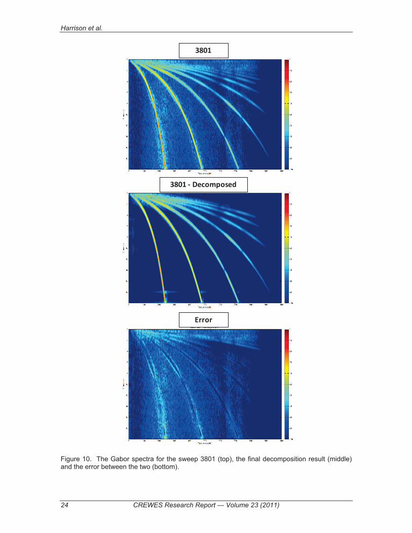
Figure 8 shows the frequency domain results of the frequency dependant Gabor decomposition with respects to the fundamental and H2 to H7. The frequency response of the original sweep, plotted in black, is modelled quite well. Figure 9 shows the Gabor spectrum of the frequency dependant Gabor decomposition with respect to the fundamental and H2 to H7. Figure 10 compares the final decomposition result with the original baseplate sweep. The Gabor plot of the error between the results and the original sweep (bottom Figure 10) shows how well the decomposition algorithm has worked. The remaining signal left on this error plot appears to be ambient noise 60 db’s down.



Figure 5. The results of time dependant Gabor decomposition of sweep 3801. (A) is time domain, (B) is frequency domain, (C) is Gabor domain. Original sweep 3801 is plotted black and analyzed sweep is plotted blue in (A) and (B). Error is plotted in red above (A) and (B).

Fund H2 H3 H4

Fund H2 H3 H4

H5

H6

Frequency (Hz)

Tim

e (s

)D

ecib

els (

db)

Am

p

Frequency (Hz)

Time (s)

A

C

H7

B

Harrison et al.


Figure 6. The results of frequency dependant Gabor decomposition of sweep 3801. (A) is time domain, (B) is frequency domain, (C) is Gabor domain. Original sweep 3801 is plotted black and analyzed sweep is plotted blue in (A) and (B). Error is plotted in red above (A) and (B).

Fund H2 H3 H4

Fund H2 H3 H4

Frequency (Hz)

Tim

e (s

)D

ecib

els (

db)

Am

p

Frequency (Hz)

Time (s)

A

C

B

H5

H6

H7



Figure 7. The individual time domain results for the frequency dependant Gabor decomposition of sweep 3801. The original sweep is plotted in black, analysis results are plotted in blue, and individual components are plotted in magenta.

Fund H2

H3 H4

H5 H6

H7

Harrison et al.


Figure 8. The individual frequency domain results for the frequency dependant Gabor decomposition of sweep 3801. The original sweep is plotted in black, analysis results are plotted in blue, and individual components are plotted in magenta. For display purposes, all frequencies are smoothed prior to plotting.



Figure 9. The individual Gabor spectra for the frequency dependant Gabor decomposition of sweep 3801.

Fund H2

H3 H4

H5 H6

H7

Harrison et al.


Figure 10. The Gabor spectra for the sweep 3801 (top), the final decomposition result (middle) and the error between the two (bottom).

3801

3801 - Decomposed

Error



Conclusion Vibroseis equipment generates a sweep using a pilot signal that varies over a designed

frequency range. Due to various mechanical factors within the Vibroseis and variances in ground coupling, this sweep also generates harmonics of these designed frequencies. Processing of Vibroseis data requires correlation or deconvolution of the raw data, which are distorted by the added harmonics. Attenuation of these harmonics has been the focus of processors and equipment engineers alike.

This paper has shown an innovative means by which the fundamental and each harmonic can be successfully decomposed from a sweep. Using Gabor analysis, broad band estimates of the fundamental and harmonics were achieved. To test this theory, synthetic and real Vibroseis sweeps were decomposed into their respective fundamental and harmonic components. The synthetic sweep, which included the fundamental to H4, each with time varying amplitude and phase, was first successfully decomposed. A recorded baseplate sweep with high signal-to-noise ratio was then tested revealing that frequency dependant Gabor decomposition (Figure 6) is presently the most accurate decomposition method. As with all seismic imaging, decomposition is ultimately reliant on data quality of the original sweep.

While the present algorithm appears to be stable, more work is required to ensure that robust sweep decomposition is reliable.

Future Work The successful decomposition of Vibroseis sweeps provides a unique opportunity to

attempt bandwidth expansion above the frequency range of the pilot sweep. As shown in Figure 3, higher frequencies from harmonic energy can readily be observed in the Gabor spectrum of traces. As stated, these frequencies associated with the harmonics have been seen as noise to be attenuated from seismic data. However, with successful decomposition, the resulting components will be used for correlation and deconvolution of the harmonically “contaminated” seismic data. The results should provide a higher frequency content seismic image revealing thinner beds.

Acknowledgements We would like to thank POTSI and CREWES for their continued support of this

project. We would also like to thank Statoil for their support and commitment to researching new and innovative technologies.

REFERENCES Abd El-Aal, A. E. K., 2011. Harmonic by harmonic removal technique for improving vibroseis data

quality: Geophysical Prospecting Vol. 59, 279-294. Gagaini, C., 2010. Acquisition and processing of simultaneous vibroseis data: Geophysical Prospecting,

Vol. 58, 81-99. Guan Yezhi, E, and Mugang, Z., 2009. A new method for analyzing vibroseis harmonics based on

overloads statistics: International Geophysical Conference & Exposition. CPS/SEG, Beijing.

Harrison et al.


Li, X. P., 1997. Decomposition of vibroseis data by the multiple filter technique: Geophysics , Vol. 62, No. 3., 980-991.

Margrave, G. F., Gibson, P.C., Grossman, J.P., Henley, D.C., and Lamoureux, M.P., 2004. Gabor deconvolution: theory and practice: EAGE. Paris France

Sercel, 2010. 428XL User's Manual Sercel. Seriff, A. J., and Kim W.H., 1970. The effect of harmonic distortion in the use of vibratory surface

sources: Geophysics, Vol. 35, No. 2, 234-246. Wei, Z., and Hall, M.A., 2011. Analyses of vibrator and geophone behavior on hard and soft ground: The

Leading Edge, Feb, 132-137 Wei, Z., Sallas, J.J., Crowell, J.M. and Teske, J.E., 2007. Harmonic distortion reduction on vibrators -

Suppressing the supply pressure ripples: 77th Annual International Meeting. SEG. San Antonio. Expanded Abstract.

APPENDIX A

Let u = 1 2( , ,..., )Nu u u , v = 1 2( , ,..., )Nv v v , w = 1 2( , ,..., )Nw w w be complex-valued time series. Choose complex parameters a, b to minimize the distance between data vector w and the linear combination au bv� . That is to minimize

( )w au bv� � (A1)

Since the distance between the two is minimized, the difference ( )w au bv� � is necessarily perpendicular to both vectors u and v. Thus using inner product notation .,. we have

( ), 0w au bv u� � � (A2)

and

( ), 0w au bv v� � � . (A3)

This yields a 2x2 system of equations for parameters a, b as

, , ,w u a u u b v u� � (A4)

and

, , ,w v a u v b v v� � . (A5)

Expressed in terms of the vector components, we have

j j j j j j

j j jw u a u u b u u� ��

(A6)

and



j j j j j j

j j jw v a u v b v v� ��

. (A7)

In the main body of this paper, for the time and frequency dependant Gabor decomposition, vectors u and v correspond to the harmonic sequences 1 2,j jg g vector w corresponds to the sweep dsjg and a, b correspond 1� and 2� . Further, for the time and frequency dependant Gabor decomposition case, vectors u and v correspond to the harmonic sequences 1 2,j jh h with respect to frequency (j) and 1 2,i ih h with respect to time (i) vector w corresponds to the sweep dsjh and a, b correspond 1� and 2� .

harmonic decomposition of a vibroseis sweep … · harmonic decomposition of a vibroseis sweep ......

Documents