harmonic current compensation applied to single-phase
TRANSCRIPT

Programa de Pos-Graduacao em Engenharia Eletrica - PPGEE
Universidade Federal de Minas Gerais - UFMG
Harmonic Current
Compensation Applied to Single-Phase
Photovoltaic Systems
Lucas Santana Xavier
Dissertacao submetida a banca examinadora designada pelo
Colegiado do Programa de Pos-Graduacao em Engenharia
Eletrica da Universidade Federal de Minas Gerais, como parte
dos requisitos necessarios para a obtencao do tıtulo de Mestre
em Engenharia Eletrica.
Orientador : Victor Flores Mendes
Coorientador : Heverton Augusto Pereira
Belo Horizonte, 15 de junho de 2018.


iii
A minha famılia,
mentores e amigos.

”Entender e transformar o que existe.”
Jiddu Krishnamurti
Agradecimentos
Primeiramente, agradeco aos meus pais, Maurıcio e Beatriz, e aos meus
irmaos, Marina e Daniel, por terem me dado todo apoio que precisei, devo
tudo a eles. Agradeco a Ana Carolina de Oliveira pelo companheirismo, me
apoiando muito nessa jornada.
Agradeco aos professores Victor Flores Mendes, Heverton Augusto Pereira
e Allan Fagner Cupertino pela paciencia e pelo imenso conhecimento cientı-
fico e de vida que obtive durante esses anos.
Agradeco aos amigos e companheiros de laboratrio, que deram muito
suporte: Victor Magno, Marcos, Valmor. Aos amigos de republica Andre
Badaia, Thiago, Joao, Jose, Rafael, Herbert. Obrigado aos integrantes do
GESEP e a todos aos meus amigos.
Agradeco aos professores do Programa de Pos-Graduacao em Engen-
haria Eletrica pelos valiosos conhecimentos que irei levar durante minha vida
profissional e transmiti-los tambem.
Agradeco a UFMG e ao LCCE/CPH por fornecer a estrutura e equipa-
mentos necessarios para a execucao deste trabalho. Agradeco a UFV, onde
me formei em Engenharia Eletrica.
v

Summary
Abstract x
List of Tables xi
List of Figures xvi
Lista de Sımbolos xix
Lista de Abreviacoes xxi
1 Introduction 1
1.1 The Distributed Generation . . . . . . . . . . . . . . . . . . . 2
1.2 PV Systems with Ancillary Services . . . . . . . . . . . . . . . 4
1.3 Motivation and Objectives . . . . . . . . . . . . . . . . . . . . 6
1.4 Methodology . . . . . . . . . . . . . . . . . . . . . . . . . . . 7
1.5 Contributions . . . . . . . . . . . . . . . . . . . . . . . . . . . 7
1.6 Text Organization . . . . . . . . . . . . . . . . . . . . . . . . . 9
2 Single-Phase PV System with Ancillary Services 10
2.1 Photovoltaic Array Modelling . . . . . . . . . . . . . . . . . . 10
2.2 Maximum Power Point Tracking . . . . . . . . . . . . . . . . . 13
2.3 DC/DC Stage Based on Boost Converter . . . . . . . . . . . . 15vii

viii
2.4 DC/AC Stage . . . . . . . . . . . . . . . . . . . . . . . . . . . 17
2.4.1 Inner Loop Control: Inverter Current Control . . . . . 18
2.4.2 Outer Loop Control: DC-Link Voltage Control . . . . 22
2.5 DC/AC Stage Control Strategy . . . . . . . . . . . . . . . . . 24
3 Selective Harmonic Current Compensation Strategy 26
3.1 Harmonic Detector Analysis . . . . . . . . . . . . . . . . . . . 32
3.1.1 SOGI Gain Effect on the Harmonic Detection . . . . . 32
3.1.2 SOGI Detection Threshold . . . . . . . . . . . . . . . . 34
3.1.3 LPF Effect on the Harmonic Detection . . . . . . . . . 36
3.1.4 SRF-PLL Natural Frequency Impact on the HarmonicDetection . . . . . . . . . . . . . . . . . . . . . . . . . 37
3.1.5 SRF-PLL Detection Threshold . . . . . . . . . . . . . . 37
3.2 Simulation Results . . . . . . . . . . . . . . . . . . . . . . . . 41
3.3 Experimental Results . . . . . . . . . . . . . . . . . . . . . . . 46
4 Partial Harmonic Current Compensation Strategy 53
4.1 Open-Loop Technique . . . . . . . . . . . . . . . . . . . . . . 54
4.2 Closed-Loop Technique . . . . . . . . . . . . . . . . . . . . . . 58
4.3 Simulation Results . . . . . . . . . . . . . . . . . . . . . . . . 61
4.4 Experimental Results . . . . . . . . . . . . . . . . . . . . . . . 68
5 Conclusions 73
5.1 Future Works . . . . . . . . . . . . . . . . . . . . . . . . . . . 74
References 75

Resumo
A geracao fotovoltaica tem crescido em todo o mundo, principalmente
na geracao distribuıda. A possibilidade de gerar energia eletrica proximo aos
centros urbanos pode reduzir os impactos de longas linhas de transmissao e
diversificar a matriz energetica de um paıs. A principal funcao do inversor
fotovoltaico e injetar a energia gerada pela planta solar na rede. Entretanto,
durante variacoes da irradiancia solar, os inversores fotovoltaicos tem uma
margem de corrente que nao e explorada. Por isso, trabalhos na literatura
tem proposto servicos auxiliares realizados por inversores fotovoltaicos. Esse
conceito e baseado em adicionar outras funcoes a estrategia de controle con-
vencional, tais como injecao de potencia reativa e compensacao de corrente
harmonica. Entretanto, um importante fato e pouco relatado na literatura
e sobre tecnicas para compensar parcialmente corrente harmonica de modo
a garantir que o inversor opere abaixo de sua corrente maxima estabelecida.
Portanto, este trabalho propoe estrategias de compensacao seletiva e par-
cial de corrente harmonica. Um metodo de deteccao de corrente harmonica
adaptativo de modo a realizar a compensacao seletiva de corrente harmonica
e duas estrategias de limitacao de corrente harmonica para compensacao
parcial de harmonicos sao introduzidos. Estudos de caso em ambiente de
simulacao e experimental sao abordados para validar a performace das es-
trategias propostas neste trabalho. Resultados mostram uma melhoria na
qualidade de energia da rede atraves da compensacao de corrente harmonica,
sem sobrecarregar o inversor fotovoltaico.
Palavras-chaves: Servicos Auxiliares, Geracao Distribuıda, Compensacao
de Corrente Harmonica, Limitacao de Corrente do Inversor, Sistemas Foto-
voltaicos.
ix
Abstract
The photovoltaic power generation have been rising around the world,
especially in the distributed generation. The possibility to generate energy
in proximity of consumer units can reduce the impacts of long transmission
lines and diversify the energy matrix of a country. The main function of
the photovoltaic inverter is to inject the power generated by the solar plant
into the electrical grid. However, due to variations in solar irradiance, in-
verters have a current margin which is not explored during the day. Hence,
some works have addressed the ancillary services provided by photovoltaic
inverters. This concept is based on adding other functions to the conven-
tional control strategy, such as reactive power injection and harmonic cur-
rent compensation. However, an important fact and less related in literature
is about techniques to compensate partially harmonic current in order to
ensure that the inverter works below its rated current. Thereby, this work
proposes strategies of selective and partial harmonic current compensation.
An adaptive harmonic current detection method in order to perform the se-
lective harmonic current compensation and two harmonic current limitation
strategies for partial harmonic compensation are introduced. Case studies in
simulation and experimental environment are addressed to validate the per-
formance of the strategies proposed here. The results show an improvement
in the grid power quality through harmonic current compensation, without
overloading the photovoltaic inverter.
Keywords: Ancillary Services, Distributed Generation, Harmonic Cur-
rent Compensation, Inverter Current Limitation, Photovoltaic Systems.
x
List of Tables
2.1 Parameters of the PV panel. . . . . . . . . . . . . . . . . . . . 13
3.1 Parameters of the boost converter. . . . . . . . . . . . . . . . 41
3.2 Parameters of the PV inverter. . . . . . . . . . . . . . . . . . . 41
3.3 power module parameters. . . . . . . . . . . . . . . . . . . . . 46
3.4 Experimental System Parameters. . . . . . . . . . . . . . . . . 46
4.1 Total demand distortion of the currents. . . . . . . . . . . . . 67
xi

List of Figures
1.1 Electricity supply by resource in Brazil (year 2018) (ANEEL,
2018). . . . . . . . . . . . . . . . . . . . . . . . . . . . . . . . 2
1.2 Power generation curve of a real PV plant during a day. . . . . 5
2.1 Generic scheme of the grid-connected photovoltaic system for
single-phase applications. . . . . . . . . . . . . . . . . . . . . . 11
2.2 Electrical model of solar cell. . . . . . . . . . . . . . . . . . . . 11
2.3 Equivalent circuit model of the DC/DC stage, PV array con-
nected to the boost converter. . . . . . . . . . . . . . . . . . . 15
2.4 Closed-loop model of the boost converter control. . . . . . . . 17
2.5 (a) Simplified illustration of the single-phase PV inverter. (b)
Inverter current control model (inner loop). . . . . . . . . . . . 19
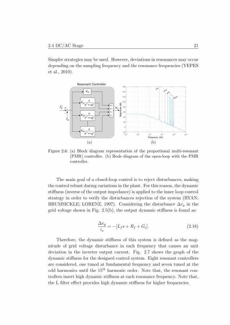
2.6 (a) Block diagram representation of the proportional multi-
resonant (PMR) controller. (b) Bode diagram of the open-loop
with the PMR controller. . . . . . . . . . . . . . . . . . . . . . 21
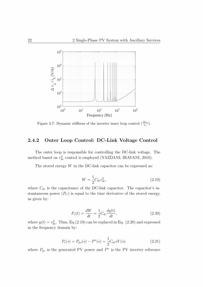
2.7 Dynamic stiffness of the inverter inner loop control (∆vgis
). . . . 22
2.8 Model of the DC-link control through v2dc based method. . . . 23
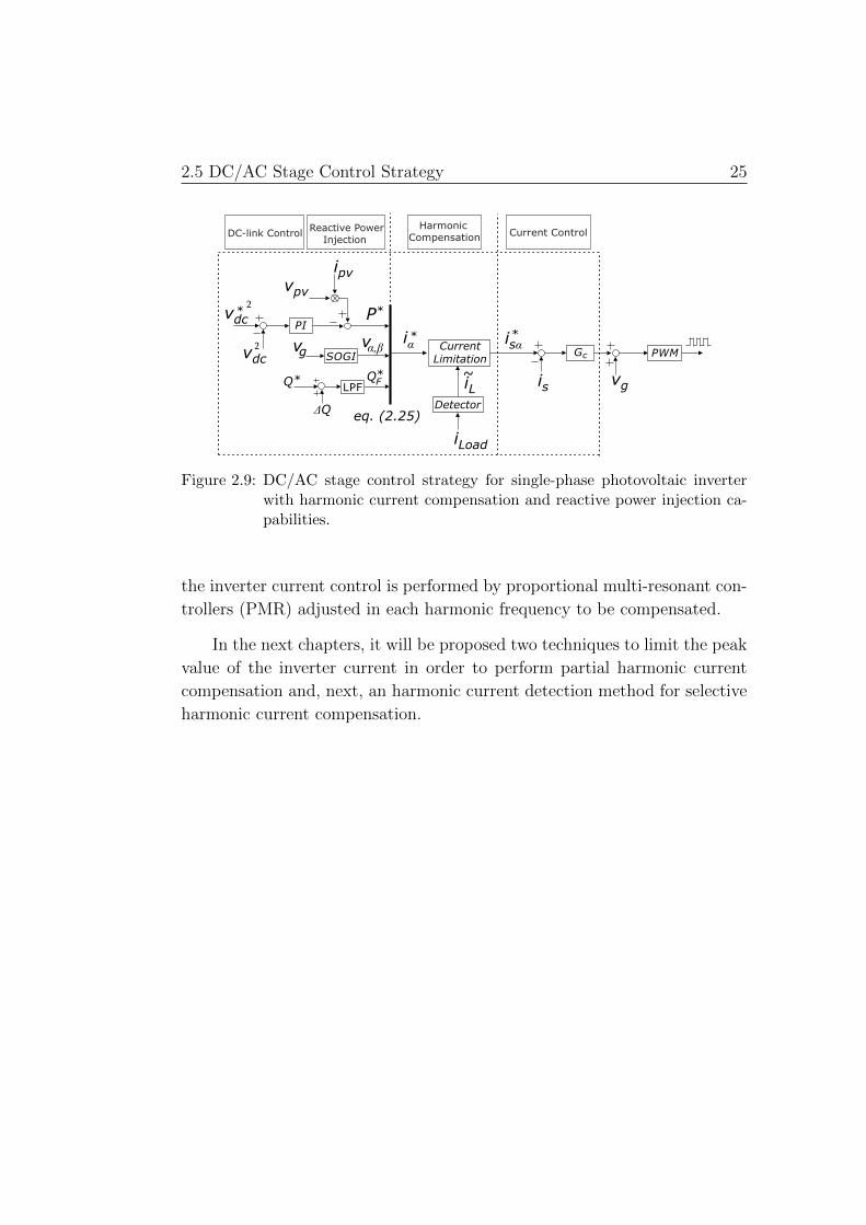
2.9 DC/AC stage control strategy for single-phase photovoltaic in-
verter with harmonic current compensation and reactive power
injection capabilities. . . . . . . . . . . . . . . . . . . . . . . . 25xii

xiii
3.1 SRF-PLL structure (KAURA; BLASKO, 1997). . . . . . . . . 28
3.2 Complete structure of the SOGI-PLL. . . . . . . . . . . . . . . 29
3.3 Bode diagrams of the SOGI for tree values of the gain k(a) Hα
transfer function. (b) Hβ transfer function. . . . . . . . . . . . 30
3.4 Current harmonic detection method based on two cascaded
SOGI-PLL. . . . . . . . . . . . . . . . . . . . . . . . . . . . . 30
3.5 Multi-stage harmonic detector. . . . . . . . . . . . . . . . . . . 32
3.6 Spectra of the iLα current for four different values of the gain
k.(a) k = 0.1.(b) k = 0.8.(c) k =√
2.(d) k = 10 . . . . . . . . 34
3.7 Magnitude of the SOGI output signals soon after the addition
of the 5th harmonic to the signal.(a) Hα magnitude gain.(b)
Hβ magnitude gain. . . . . . . . . . . . . . . . . . . . . . . . . 35
3.8 5th harmonic component detection response for two different
values of I5. . . . . . . . . . . . . . . . . . . . . . . . . . . . . 36
3.9 Detected frequency and amplitude for three different values
for both cut-off frequencies (fcf and fca) of the LPFs, consid-
ering k =√
2.(a) Detected frequency for three fcf values.(b)
Detected amplitude for three fca, keeping fcf = 10 Hz.(c)
Detected amplitude spectrum for three fca values, keeping
fcf = 10 Hz. (d) Detected iL current spectrum, parameters:
fca = 30 Hz, fcf = 10 Hz and k =√
2 . . . . . . . . . . . . . 38
3.10 Detected frequency and amplitude for some values of SRF-
PLL natural frequency fn. Parameters: k =√
2, fca = 5 Hz
and fcf = 10 Hz.(a) Detected frequency.(b) Detected amplitude. 39
3.11 SRF-PLL detection threshold in function of ξ and ωn consid-
ering a transition from 3rd to 5th harmonic order. . . . . . . . 40
3.12 Current spectra of two nonlinear loads used in the simulation
case study. (a) Load 1. (b) Load 2. . . . . . . . . . . . . . . . 42

xiv
3.13 Detected harmonic current components of the load current
using the SOGI-PLL structure. (a) Fundamental current peak
detected in stage 1. (b) Detected fundamental frequency.(c)
Predominant harmonic current peak detected in stage 2. (d)
Detected frequency of the predominant harmonic. (e) Current
peak of the second predominant harmonic current detected in
stage 3. (f) Detected frequency of the second predominant
harmonic. . . . . . . . . . . . . . . . . . . . . . . . . . . . . . 44
3.14 Detected current spectrum. (a) Load 1. (b) Load 2 . . . . . . 45
3.15 Spectra of the load (iLoad), inverter (is) and grid (ig) current
in steady state before and after the load change in 1.4 seconds
. (a) Before 1.4 seconds. (b) After 1.4 seconds . . . . . . . . . 45
3.16 Setup of the designed prototype. (a) Setup overview: 1- Power
module. 2- Control circuit. 3- Conditioning and control boards.
4- Microcomputer. (b) Conditioning and control boards. . . . 47
3.17 Schematic of the designed nonlinear load. . . . . . . . . . . . . 48
3.18 Designed nonlinear load. (a) Setup overview. (b) Setup inside
view. . . . . . . . . . . . . . . . . . . . . . . . . . . . . . . . 48
3.19 Current spectra of two nonlinear loads used in this experimen-
tal case study. (a) Load 1. (b) Load 2. . . . . . . . . . . . . . 48
3.20 Detection of the fundamental component performed by the
first stage of the harmonic current detector. (a) Amplitude.
(b) Frequency. . . . . . . . . . . . . . . . . . . . . . . . . . . . 49
3.21 Detection of the predominant harmonic component performed
by the second stage of the harmonic current detector. (a)
Amplitude. (b) Frequency. . . . . . . . . . . . . . . . . . . . . 50
3.22 Detection of the second predominant harmonic component
performed by the third stage of the harmonic current detector.
(a) Amplitude. (b) Frequency. . . . . . . . . . . . . . . . . . . 51
3.23 Current waveforms and spectra during harmonic compensa-
tion of the load 1. . . . . . . . . . . . . . . . . . . . . . . . . . 51
xv
3.24 Current waveforms and current spectra during harmonic com-
pensation of the load 2. . . . . . . . . . . . . . . . . . . . . . . 52
4.1 Inverter current limitation technique based on open-loop algo-
rithm. . . . . . . . . . . . . . . . . . . . . . . . . . . . . . . . 54
4.2 Flowchart of the harmonic current limitation (HCL) algorithm. 55
4.3 Details of waveforms of the currents during harmonic current
compensation. (a) Total inverter current reference (i∗st), i.e,
without Kh factor action. (b) Inverter current reference (i∗sα),
i.e, with Kh factor action. . . . . . . . . . . . . . . . . . . . . 57
4.4 Inverter current limitation technique based on PI controller. . 58
4.5 Closed-loop control modeling of the current limitation tech-
nique based on PI controller. . . . . . . . . . . . . . . . . . . . 59
4.6 Disturbance rejection analysis through the step response of
the E(s) transfer function. . . . . . . . . . . . . . . . . . . . . 60
4.7 Kh factor calculation comparison between the two techniques
for inverter current limitation and the model of the closed-loop
technique. (a) Time response of the Kh factor. (b) Steady-
state response of the Kh factor in relation to the fundamental
current reference injected by the inverter. . . . . . . . . . . . . 61
4.8 Current spectra of two nonlinear loads used in the simulation
case study. (a) Load 1. (b) Load 2. . . . . . . . . . . . . . . . 62
4.9 Voltage and current dynamics of the PV system DC-side. (a)
Output PV array voltage (vpv). (b) Inductor current of the
boost converter. (c) Dc-link voltage vdc. . . . . . . . . . . . . . 63
4.10 Dynamic of the active power (P) and reactive power (Q) flow
on the system. (a) Active power. (b) Reactive power. . . . . . 64
4.11 Compensation factor Kh using two techniques for inverter cur-
rent limitation. . . . . . . . . . . . . . . . . . . . . . . . . . . 65

xvi
4.12 Inverter current waveform details during transient responses.(a)
Transient response at 1 s. (b) Transient response at t = 0.6
seconds. (b) Transient response at t = 1 second. (c) Transient
response at t = 1.4 seconds. (d) Transient response at t = 1.8
seconds. (e) Transient response at t = 2.2 seconds. . . . . . . . 66
4.13 Inverter current space phasor. (a) Without harmonic current
limitation technique. (b) With harmonic current limitation
technique. . . . . . . . . . . . . . . . . . . . . . . . . . . . . . 67
4.14 Experimental compensation factor Kh using two techniques
for inverter current limitation. . . . . . . . . . . . . . . . . . . 69
4.15 Current waveforms and spectra of the system during harmonic
compensation with inverter current limitation based on open-
loop technique. (a) 0 < t < 1.5 seconds. (b) 1.5 < t < 3.0
seconds. (c) 3.0 < t < 4.5 seconds. (d) 4.5 < t < 6 seconds. . . 71
4.16 Current waveforms and spectra of the system during harmonic
compensation with inverter current limitation based on closed-
loop technique. (a) 0 < t < 1.5 seconds. (b) 1.5 < t < 3.0
seconds. (c) 3.0 < t < 4.5 seconds. (d) 4.5 < t < 6 seconds. . . 72

Symbol List
Cpv Photovoltaic array output capacitance
Cdc DC-link capacitance
Lb Boost converter inductance
Li Inverter side inductance of the LCL filter
Lg Grid side inductance of the LCL filter
Lf Equivalent inductance of the inverter filter
Rb Equivalent series resistance of the boost converter inductor
Rf Equivalent series resistance of the inverter filter
RS Series resistance of the photovoltaic array
RP Parallel resistance of the photovoltaic array
Rmpp Output Resistance of the photovoltaic array at the maximum power point
ipv Current generated by photovoltaic array
is Inverter current
i∗s Inverter current reference
ig Grid current
iL Load current and boost inductor current
iL Harmonic current
io Leakage current of the photovoltaic array model
isc Short-circuit current of the photovoltaic panel
impp Maximum power point current of the photovoltaic panel
Ih Harmonic current amplitude
If Fundamental current amplitude
Im Peak value of the inverter current reference
I∗m Inverter rated current
xvii

xviii
Iα Fundamental component contribution to the inverter current peak value
IL Harmonic component contribution to the inverter peak value
vpv Photovoltaic string output voltage
vdc DC-link voltage
vg Grid voltage
vt Panel thermal voltage of the photovoltaic array model
voc Open-circuit voltage of the photovoltaic panel
vmpp Voltage at maximum power point of the photovoltaic panel
d Duty cycle of the boost converter
ωo Initial angular frequency of the harmonic current detector
ωn PLL Natural angular frequency
ωh Harmonic angular frequency
ωf Fundamental angular frequency
ff Fundamental frequency
fs switching frequency
fn PLL natural frequency
fcf Cut-off frequencies of the low-pass filter
fca Cut-off frequencies of the low-pass filter
t Time
Ts Sampling period
To Half period of the fundamental period
ζ PLL Damping factor
k SOGI gain
Kh Harmonic compensation factor
W Energy
Q Reactive power
Q∗ Reactive power reference injected by photovoltaic system
P Active power
P ∗ Active power reference injected by photovoltaic system
Pmp Maximum power of the photovoltaic array
S Apparent power
S∗ Apparent power reference injected by photovoltaic system
Sm Inverter rated Apparent power
ns Number of cells in series
a Diode ideality constant of the photovoltaic array model
k Boltzmann constant
T Temperature of the photovoltaic panel
G Solar Irradiance
Kv Temperature coefficient of the photovoltaic array model
Ki Temperature coefficient of the photovoltaic array model

xix
Kpbi Proportional gain of the inner loop of the boost converter control
Kibi Integral gain of the inner loop of the boost converter control
Kpbv Proportional gain of the outer loop of the boost converter control
Kibv Integral gain of the outer loop of the boost converter control
Kp,pll Proportional gain of the PLL control
Ki,pll Integral gain of the PLL control
Kp Proportional gain of the multi-resonant controller
Kih Resonant gains of the multi-resonant controller
Kpsv Proportional gain of the v2dc control based method
Kisv Integral gain of the v2dc control based method
Kp,sat Proportional gain of the current limitation strategy based on closed-loop
Ki,sat Integral gain of the current limitation strategy based on closed-loop
Superscripts
∗ Reference value
Subscribers
α quantities referred to the stationary reference-frame
β quantities referred to the stationary reference-frame
d quantities referred to the synchronous reference-frame
q quantities referred to the synchronous reference-frame

List of Acronyms
ANEEL Agencia Nacional de Energia Eletrica
DG Distributed Generation
ICMS Imposto Sobre Circulacao de Mercadorias e Servicos
PV Photovoltaic
DC Direct Current
AC Alternating Current
MPPT Maximum Power Point Tracking
MPP Maximum Power Point
P&O Perturbation and Observation
PI Proportional and Integral
PCC Point of Common Coupling
xx
xxi
THD Total Harmonic Distortion
TDD Total Demand Distortion
SRF-PLL Syncronous Reference Frame-Phase-locked loop
SOGI Second Order Generalized Integrator
PMR Proportional Multi-Resonant
RPC Repetitive Controller
FLL Frequency Locked Loop
DFT Discrete Fourier Transform
LPF Low-Pass Filter
RMS Root Mean Square
CCVT Current Contribution Value Tracking
HCL Harmonic Current Limitation
HC Harmonic Compensation

Chapter 1
Introduction
Brazil has structured its power generation system based on hydraulic
power plants since the end of the 19th century, when the first hydroelectric
power plant started to operate in Diamantina (CEMIG, 2012). The impor-
tance of the hydroelectric power plants in the structural change and economic
development of the Brazil in the last 100 years is evident. On the other hand,
the Brazilian electrical power system became very dependent on this type of
resource.
Since 2011, Brazil is facing an intense water scarcity in several regions,
including places where important hydroelectric power stations are installed.
As results, thermoelectric power plants are increasing the generation capacity
with concern to save water in hydroelectric stations reservoirs (PINTO et al.,
2015). However, the generated electric energy based on thermoelectric power
plants is at least twice as expensive as based on hydraulic processes, besides
injecting greenhouse gases into the atmosphere.
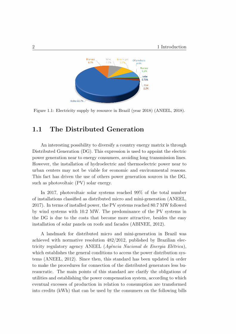
It is a consensus that Brazil has diversified its electric energy sources in
the last 15 years. However, data from 2018 show that hydraulic generation
accounts for 60.7% of supply, as shown in Fig. 1.1 (ANEEL, 2018). The
solar, wind and biomass sources are only responsible for 0.75%, 7.7% and
8.7% of supply, respectively, although the data shows that Brazil presents
an electricity matrix predominantly renewable. Although most economic
indicators appoint that renewable energy sources may occupy a significant
share of the world’s energy matrix, the projections for installations in Brazil
are far below when compared with countries such as China, Germany, United
States, Japan, Indian and other countries (REN21, 2017).
2 1 Introduction
Figure 1.1: Electricity supply by resource in Brazil (year 2018) (ANEEL, 2018).
1.1 The Distributed Generation
An interesting possibility to diversify a country energy matrix is through
Distributed Generation (DG). This expression is used to appoint the electric
power generation near to energy consumers, avoiding long transmission lines.
However, the installation of hydroelectric and thermoelectric power near to
urban centers may not be viable for economic and environmental reasons.
This fact has driven the use of others power generation sources in the DG,
such as photovoltaic (PV) solar energy.
In 2017, photovoltaic solar systems reached 99% of the total number
of installations classified as distributed micro and mini-generation (ANEEL,
2017). In terms of installed power, the PV systems reached 80.7 MW followed
by wind systems with 10.2 MW. The predominance of the PV systems in
the DG is due to the costs that become more attractive, besides the easy
installation of solar panels on roofs and facades (ABINEE, 2012).
A landmark for distributed micro and mini-generation in Brazil was
achieved with normative resolution 482/2012, published by Brazilian elec-
tricity regulatory agency ANEEL (Agencia Nacional de Energia Eletrica),
which establishes the general conditions to access the power distribution sys-
tems (ANEEL, 2012). Since then, this standard has been updated in order
to make the procedures for connection of the distributed generators less bu-
reaucratic. The main points of this standard are clarify the obligations of
utilities and establishing the power compensation system, according to which
eventual excesses of production in relation to consumption are transformed
into credits (kWh) that can be used by the consumers on the following bills

1.1 The Distributed Generation 3
up to (60 months ahead).
Brazil has extended the economic incentives for PV installations in the
last years. Most Brazilian states have already exempt the tax on circulation
of goods and transportation and communication services ICMS (Imposto So-
bre Circulacao de Mercadorias e Servicos) from photovoltaic systems. In
addition, national banks are providing credit line for the PV sector. These
incentives are very favorable to the energy consumers who want to have their
DG. However, from the point of view of utilities, the growth of PV system in
distributed micro and mini-generation is being seen as a threat, mainly due
to the following factors (ABINEE, 2012):
• Possible revenue loss of companies due to the energy consumers growth
using the power compensation system;
• The solar energy is a non-dispatchable source of electricity. Thus, it
can not turn the solar panels on the same way that can ramp up central
coal and hydro plants to match power demand.
These challenges are common in countries that have experienced the ex-
pansion of renewable energy sources in their electrical power systems. For
example, Germany’s biggest power companies, which were based on the elec-
tricity generation from nuclear, coal and oil sources became unprofitable with
the expansion of solar and wind power in the country. To overcome this draw-
back, most of them were split into two companies, one for renewable energy
and new services and one for conventional energy. In addition, most of these
utilities mainly invest in renewable abroad. These strategies were adopted by
the Germany’s energy firms to survive in the new energy scenario (MORRIS;
PEHNT, 2012).
The currently generation systems are balanced with the demand. This
energy production mode is not compatible with the photovoltaic generation.
Thus, several energy storage solutions are being studied and tested to over-
come this challenge such as underground compressed air in natural caverns to
pumped storage, flywheels, and batteries, in order to have a flexible system
of energy production (MORRIS; PEHNT, 2012).
Despite all these challenges, PV systems can contribute for a smarter
electrical system. For long time, PV installations were only considered as

4 1 Introduction
active power generators. However, this perception has been changing. In
fact, these systems can contribute to the grid operation through ancillary
services and this will be discussed in this work.
1.2 PV Systems with Ancillary Services
The discussion about the potential to use the DG to provided ancillary
services has intensified from the early 2000s due mainly to the technological
advances in electrical and mechanical power conversion systems (JOOS et al.,
2000), (PEPERMANS et al., 2005). At the same time, the IEEE Standard
1547 was raised for interconnecting distributed resources with electric power
systems. This standard also defines the ancillary services in distributed power
generation systems such as load regulation, energy losses, spinning and non-
spinning reserves, voltage regulation, and reactive-power supply. The number
of PV plants connected to low-voltage distribution lines has been increasing
in the later years. Hence, the use of the PV systems to perform ancillary
services have attracted attention from researchers (MASTROMAURO et al.,
2009), (YANG, 2014).
These ancillary services that PV systems can performed are still being
ignored or poorly detailed by most grid codes. However, in a wide-scale pen-
etration scenario of PV systems in the distributed grid, the effects of inter-
mittent power generation of this source can not be ignored. Thus, countries
grid codes should be updated in the near future, aiming grid protection and
support functionality, flexible power controllability and intelligent ancillary
services (YANG, 2014). This demand reinforces the importance of research
about the next generation of PV system.
In grid-connected PV systems, there are power electronic inverters in-
jecting the energy extracted from the photovoltaic array into the alternating
current (AC) grid. Today, this electronic device can be connected to the
single-phase or three-phase power systems without transformers, reducing
the weight and volume of the equipment (KJAER; PEDERSEN; BLAAB-
JERG, 2005), (KEREKES et al., 2009). The single-phase PV inverters are
commonly used for applications up to 7 kW. Above this value, three-phase
inverters are usually recommended.
1.2 PV Systems with Ancillary Services 5
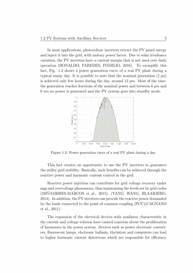
In most applications, photovoltaic inverters extract the PV panel energy
and inject it into the grid, with unitary power factor. Due to solar irradiance
variation, the PV inverters have a current margin that is not used over daily
operation (BONALDO; PAREDES; POMILIO, 2016). To exemplify this
fact, Fig. 1.2 shows a power generation curve of a real PV plant during a
typical sunny day. It is possible to note that the nominal generation (1 pu)
is achieved only few hours during the day, around 12 pm. Most of the time,
the generation reaches fractions of the nominal power and between 6 pm and
6 am no power is generated and the PV system goes into standby mode.
Figure 1.2: Power generation curve of a real PV plant during a day.
This fact creates an opportunity to use the PV inverters to guarantee
the utility grid stability. Basically, such benefits can be achieved through the
reactive power and harmonic content control in the grid.
Reactive power injection can contribute for grid voltage recovery under
sags and overvoltage phenomena, thus maintaining the levels set by grid codes
(MINAMBRES-MARCOS et al., 2015), (YANG; WANG; BLAABJERG,
2014). In addition, the PV inverters can provide the reactive power demanded
by the loads connected to the point of common coupling (PCC)(CAGNANO
et al., 2011).
The expansion of the electrical devices with nonlinear characteristic in
the current and voltage relation have caused concerns about the proliferation
of harmonics in the power system. Devices such as power electronic convert-
ers, fluorescent lamps, electronic ballasts, thyristors and computers can lead
to higher harmonic current distortions which are responsible for efficiency

6 1 Introduction
reduction of the power grid, besides interacting with resonances present in
the system (De la Rosa, 2006). For this reason, several works have proposed
to use photovoltaic systems to mitigate current and voltage harmonic dis-
tortions generated by nonlinear loads (XAVIER; CUPERTINO; PEREIRA,
2014), (BONALDO; PAREDES; POMILIO, 2016), (HE; LI; MUNIR, 2012),
(PAREDES et al., 2015)
These ancillary services that PV systems can performed are still being
ignored or poorly detailed by most grid codes. However, in a wide-scale pen-
etration scenario of PV systems in the distributed grid, the effects of inter-
mittent power generation of this source can not be ignored. Thus, countries
grid codes should be updated in the near future, aiming grid protection and
support functionality, flexible power controllability and intelligent ancillary
services (YANG, 2014). This demand reinforces the importance of researches
about the next generation of PV system.
1.3 Motivation and Objectives
Generally, the PV system sizing must be in such way that the inverter
does not operate far below its rated power most of the time but also without
overload conditions, in order to get the best cost and benefit of the system
(PINHO; GALDINO, 2014). In such conditions, over sizing a small photo-
voltaic system to perform ancillary services is not a very attractive idea, once
this can greatly increase the system cost.
Therefore, an interesting alternative is to maintain the sizing methodol-
ogy of PV systems based on the total power of PV panels installed and use the
ancillary services within this projected power range. Thus, the photovoltaic
inverters act to assist the grid within their power capacity at that given mo-
ment. Two ways to perform harmonic current compensation, respecting the
capacities of the PV inverter, are proposed by this work.
Firstly, the inverter switches have a current limit that cannot be ex-
ceeded, to preserve its lifetime and safety. The critical point is when har-
monic current compensation is involved (PEREIRA et al., 2015). In this
situation there are multiple frequencies in the current signal and analytical
expressions for inverter current limitation are complex. In addition, limiting

1.4 Methodology 7
the RMS current when there are multiple harmonic orders in the signal is not
effective, since the current peak can be much larger than its RMS value. For
this reason. The present work intends to scrutinize techniques to limit the
peak value of the PV inverter in order to perform partial harmonic current
compensation using single-phase PV systems.
Second, nonlinear load currents present several harmonic components
and compensate all these components can exceed the physical and control
capability of the PV inverter (LASCU et al., 2009). For this reason, this work
intends to scrutinize a method for selective harmonic current compensation,
where only some predominant harmonics are detected and compensated.
1.4 Methodology
The methodology to achieve these goals is:
• Mathematical modeling in time and frequency domain in order to de-
scribe parameters for the method and techniques proposed in this work
and for the PV system control;
• Simulation results in PLECS environment using computational model
presenting relevant dynamics of the PV system;
• Experimental validation of the proposed method and techniques through
a prototype system built in the laboratory.
1.5 Contributions
In view of the above discussions, the main contributions of this work are:
• Propose a harmonic current detection method to perform selective har-
monic current compensation;
• Propose harmonic current limitation techniques for partial harmonic
current compensation by reducing the PV inverter current peak.

8 1 Introduction
The results produced in this work originated two conference papers and
one paper in a journal. They are cited below per chronological order:
• L. S. Xavier, A. F. Cupertino, V. F. Mendes and H. A. Pereira, ”Detec-
tion method for multi-harmonic current compensation applied in three-
phase photovoltaic inverters,” 12th IEEE International Conference on
Industry Applications (INDUSCON), Curitiba, 2016, pp. 1-8.
• L. S. Xavier, A. F. Cupertino, J. T. de Resende, V. F. Mendes, H. A.
Pereira, ”Adaptive current control strategy for harmonic compensation
in single-phase solar inverters, Electric Power Systems Research, vol.
142, 2017, pp. 84-95.
• L. S. Xavier, V. M. R. de Jesus, A. F. Cupertino, V. F. Mendes and H.
A. Pereira, ”Novel adaptive saturation scheme for photovoltaic invert-
ers with ancillary service capability,” 8th International Symposium on
Power Electronics for Distributed Generation Systems (PEDG), Flori-
anopolis, 2017, pp. 1-8.
The published conference papers in correlated topics are cited below per
chronological order:
• V. M. R. de Jesus, L. S. Xavier, A. F. Cupertino, H. A. Pereira and V. F.
Mendes, ”Comparison of MPPT strategies applied in three-phase pho-
tovoltaic inverters during harmonic current compensation”, 12th IEEE
International Conference on Industry Applications (INDUSCON), Cu-
ritiba, 2016, pp. 1-8.
• V. M. R. de Jesus, L. S. Xavier, A. F. Cupertino, V. F. Mendes and
H. A. Pereira. Operating limits of three-phase multifunctional pho-
tovoltaic converters applied for harmonic current compensation, 8th
International Symposium on Power Electronics for Distributed Gener-
ation Systems (PEDG), Florianopolis, 2017, pp. 1-8.

1.6 Text Organization 9
1.6 Text Organization
In this first chapter an overview of the use of PV system in DG was pre-
sented and several ancillary services were briefly described. The motivation
and objectives of this work were clarified, as well as the methodology used
in order to reach these aims. Finally, the intended contributions were set.
The second chapter describes the main control structures used in this
work. The mathematical model of each structure are presented as well.
In the third chapter, a harmonic current detection method is proposed
for selective harmonic current compensation. In fourth chapter, techniques
for partial harmonic current compensation are introduced.
In the last chapter the conclusions are presented and the proposals for
continuation are listed.

Chapter 2
Single-Phase PV System with
Ancillary Services
In this chapter, an overview on the basic and advanced functions of the
single-phase PV system is described and presented in Fig. 2.1.
In addition to the basic functions, the focus is the harmonic current
compensation and the reactive power injection. Fig. 2.1 shows that the
system connection for basic and advanced functions are similar. However, to
include in the PV inverters the capability to perform reactive power injection
and harmonic current compensation, additional current sensor is necessary
to detect the load current, mainly if the control strategy is performed by
current controllers. For these purposes, the load current information is taken
from the sum between the grid current and the inverter current. This ensures
that the current information of all loads connected to the PCC is achieved.
2.1 Photovoltaic Array Modelling
The devices responsible for photovoltaic conversion are solar cells. These
structures can be represented as a diode with its p-n junction exposed to irra-
diance (RAUSCHENBACH, 1980). The typical PV silicon cells can generate
power ranging from 1 W to 2 W, approximately. Thereby, in practical and
commercial applications, solar cells are associated in series or parallel, form-
ing the PV modules.
The ideal PV cell can be represented by a direct current source (ipv) in

2.1 Photovoltaic Array Modelling 11
Figure 2.1: Generic scheme of the grid-connected photovoltaic system for single-phase applications.
parallel with the diode. This representation describes the I-V characteris-
tics of an ideal PV cell. However, the equivalent series (RS) and parallel
resistances (RP ) are added to increase the accuracy of the PV array model.
These resistances depend on the contact resistance of the metal base with
the semiconductor layers and on the leakage current of the p-n junction.
A PV array can be represented by the electrical equivalent circuit shown
in Fig. 2.2. Thereby, from the semiconductor physics, the generated current
from the PV cell terminals (i) can be represented by the following expression
(RAUSCHENBACH, 1980):
Load
PV c modelell
ilg
id
RS
RP v R
i
Co
Figure 2.2: Electrical model of solar cell.
i = ilg − i0[exp
(v +Rsi
vta
)− 1
]− v +Rsi
Rp
, (2.1)
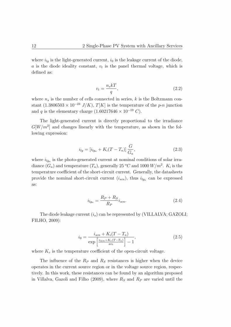
12 2 Single-Phase PV System with Ancillary Services
where ilg is the light-generated current, i0 is the leakage current of the diode,
a is the diode ideality constant, vt is the panel thermal voltage, which is
defined as:
vt =nskT
q, (2.2)
where ns is the number of cells connected in series, k is the Boltzmann con-
stant (1.3806503× 10⁻²³ J/K), T [K] is the temperature of the p-n junction
and q is the elementary charge (1.60217646× 10⁻¹⁹ C).
The light-generated current is directly proportional to the irradiance
G[W/m2] and changes linearly with the temperature, as shown in the fol-
lowing expression:
ilg = [ilgn +Ki(T − Tn)]G
Gn
, (2.3)
where ilgn is the photo-generated current at nominal conditions of solar irra-
diance (Gn) and temperature (Tn), generally 25 oC and 1000 W/m2. Ki is the
temperature coefficient of the short-circuit current. Generally, the datasheets
provide the nominal short-circuit current (iscn), thus ilgn can be expressed
as:
ilgn =RP +RS
RP
iscn. (2.4)
The diode leakage current (io) can be represented by (VILLALVA; GAZOLI;
FILHO, 2009):
i0 =iscn +Ki(T − Tn)
exp[vocn+Kv(T−Tn)
avt
]− 1
, (2.5)
where Kv is the temperature coefficient of the open-circuit voltage.
The influence of the RP and RS resistances is higher when the device
operates in the current source region or in the voltage source region, respec-
tively. In this work, these resistances can be found by an algorithm proposed
in Villalva, Gazoli and Filho (2009), where RS and RP are varied until the

2.2 Maximum Power Point Tracking 13
maximum power calculated by the solar panel model becomes equal to the
maximum power from datasheet at the maximum power point.
This mathematical model of the PV array is used in the case study
simulations to validate the methodology presented in this work for partial
harmonic compensation and reactive power injection using a single-phase
PV system. The main parameters used in the mathematical model approach
can be found in most photovoltaic panels datasheets.
In this work, a traditional commercial PV panel of 250 W is used in
order to form the PV array. The parameters of this panel under standard
test conditions (STC) (1000 W/m2 and module temperature 25 C,) are
presented in Table 2.1. The simulated PV array is composed for 2 strings
with 6 panels in series in each branch, resulting in a generated power at
maximum power point equal to 3 kW .
Table 2.1: Parameters of the PV panel.
Parameter ValueMaximum power (Pmpp) 250 WOpen-circuit voltage (voc) 37.5 VShort-circuit current (isc) 8.5 AVoltage at maximum power point (vmpp) 31.29 VCurrent at maximum power point (impp) 7.99 ATemperature coefficient of Voc (Kv) −0.313 %/oCTemperature coefficient of Isc (Ki) 0.0043 %/oCNumber of cells in series (ns) 60Nominal irradiance (Gn) 1000 W/m2
Nominal operation temperature (Tn) 320 KPanel series resistance (Rs) 0.173900 ΩPanel parallel resistance (Rp) 379.023365 Ω
2.2 Maximum Power Point Tracking
Since 1993, the conversion efficiency of solar irradiance in electricity
through multicrystalline silicon solar cells improved from 18% to 22.3% (GREEN
et al., 2018). This is not a small difference in terms of PV cells, besides, this
shows that it is very difficult to increase 1% in the energy conversion effi-
ciency even with technological advances. There are new and more efficient

14 2 Single-Phase PV System with Ancillary Services
PV cells technologies, such as GaInP/GaAs multijunction. However, these
cells are still impractical in the market due to their high manufacturing cost.
The generated power from the solar cell depends on its temperature, the
solar irradiance and the electrical characteristics of the load. For this rea-
son, the maximum power extraction is an important issue in PV generation.
This goal is achieved through the maximum power point tracking (MPPT)
algorithms.
Due to low algorithm complexity and low computational power require-
ment, the most traditional MPPT method is the Perturbation and Observa-
tion (P&O) (HUSSEIN et al., 1995). This algorithm periodically increments
or decrements the solar string voltage and compares the output power with
the previous value. If the delivered power is increased, the solar array voltage
perturbation will continue in the same direction. When the supplied power
starts to decrease, the system reaches the maximum power point (MPP) and
the P&O algorithm output oscillates around that point. Other traditional
MPPT algorithm is the incremental conductance based method, a specific
implementation of the P&O (HUSSEIN et al., 1995). This algorithm evalu-
ates of the incremental conductance (di/dv) in each interaction period.
However, in cases of rapidly changing atmospheric conditions, the P&O
algorithm can track in the wrong direction in relation to the MPP and it can
cause a reduction of efficiency. This can happen when the power variation,
due to solar irradiance variation, is higher than the caused by the algorithm
action. Thereby, the algorithm interprets the power variation only as an
effect of its own action. Hence, dP -P&O method is proposed in literature in
order to solve problems caused by the rapidly changing in irradiance (SERA
et al., 2008).
To solve the P&O problem during rapidly change in the solar irradiance,
the dP -P&O method determines the correct tracking by means of additional
power measurement at the middle of the MPPT sampling period without
any perturbation. Thereby, during rapidly change in the solar irradiance,
the action of this MPPT is able to interpret correctly if the power change is
caused as an effect of its own action or due to solar irradiance change (SERA
et al., 2008). In this work, the dP -P&O algorithm is used.

2.3 DC/DC Stage Based on Boost Converter 15
2.3 DC/DC Stage Based on Boost Converter
The DC/DC stage converter is commonly used to boost the input voltage
level of the inverter, ensuring the acceptable voltage level for startup and
extending its operation range during low irradiance conditions. In single-
phase systems, the use of DC/DC is even more important due to power
oscillation in the 2nd harmonic frequency. This power oscillation results in
DC-link voltage fluctuation and reduces the efficiency of the MPPT algorithm
if PV modules are connected directly to the DC-link. For this reason, it
is advisable to perform the MPPT algorithm in the DC/DC stage control
for single-phase applications. The boost converter is widely used for these
purposes (BLAABJERG et al., 2006),(YANG; ZHOU; BLAABJERG, 2015)
The connection of the PV array to the boost converter is shown in Fig.
2.3. The PV array model is linearized around the nominal maximum power
point, since the operation of the device should occur preferably around this
point (VILLALVA; SIQUEIRA; RUPPERT, 2010). Therefore, the PV array
can be modeled by a linear circuit composed of an equivalent voltage source
(vmpp) and corresponding the resistance (Rmpp) at MPP. The DC-link can be
represented by a voltage source (v∗dc), assuming that the voltage is already
controlled by the following stage. The average values of the capacitor voltage
(vpv) and inductor current (iLb) over one switching period can be obtained
as respectively:
vmpp Cpvvdc
RbRmpp
vpv
iLb
PV array model
S
Lbipv
*
Figure 2.3: Equivalent circuit model of the DC/DC stage, PV array connected tothe boost converter.
Cpvd〈vpv〉dt
=vmppRmpp
− 〈vpv〉Rmpp
− 〈iLb〉, (2.6)
16 2 Single-Phase PV System with Ancillary Services
Lbd〈iLb〉dt
= 〈iL〉Rb + (1− d)v∗dc − 〈vpv〉, (2.7)
where Rb is the inductor equivalent series resistance and d is the duty cycle.
The goal is to find two transfer functions in the frequency domain,
relating Gvi(s) = vpv/iLb and Gid(s) = iLb/d. A small-signal approach
is adopted to linearize the converter model (ERICKSON; MAKSIMOVIC,
2001). Therefore, Eq. (2.6) and (2.7) are rewritten in the frequency domain
as:
vpv(s) = − 1
sCpvRmpp
vpv(s)−1
sCpviLb(s), (2.8)
iLb(s) =Rb
sLbiLb(s) +
v∗dcsLb
d(s)− 1
sLbvpv(s), (2.9)
where “ˆ” means a small-signal term. From Eq. (2.8) and (2.9) the trans-
fer functions, which represent the relationship between Gvi and Gid, can be
obtained as:
Gvi(s) =vpv
iLb= − 1
sCpv + 1Rmpp
, (2.10)
Gid(s) =iLb
d=
v∗dcsLb +Rb
, (2.11)
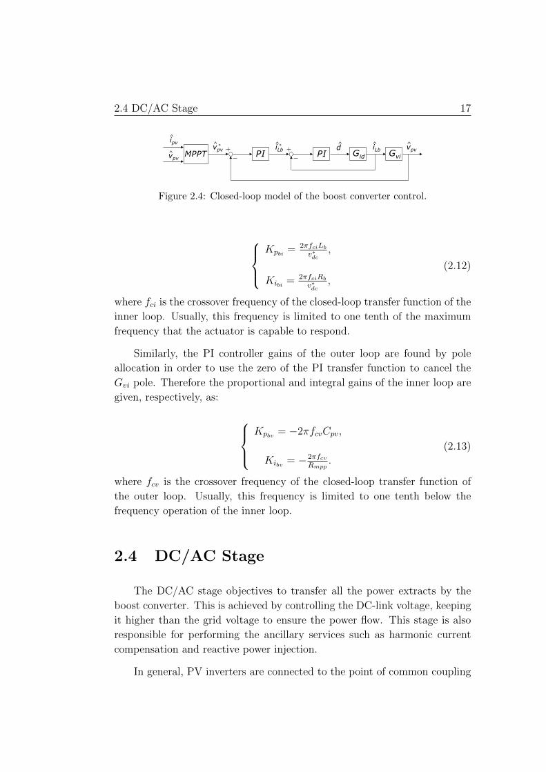
Therefore, the closed-loop model of the boost converter control based on
proportional-integral (PI) controllers is illustrated in Fig. 2.4. The boost
converter control loop consists of an outer loop responsible for controlling
the solar array output voltage (vpv) and an inner loop tuned to regulate the
boost converter inductor current (iLb). The voltage reference of the outer
loop is calculated by the MPPT algorithm.
The proportional and integral gains of the PI controller of the inductor
current control loop are adjusted by pole allocation to use the zero of the
PI transfer function to cancel the Gid pole. Therefore, the proportional and
integral gains of the inner loop are given, respectively, as:
2.4 DC/AC Stage 17
Figure 2.4: Closed-loop model of the boost converter control.
Kpbi = 2πfciLb
v∗dc,
Kibi = 2πfciRb
v∗dc,
(2.12)
where fci is the crossover frequency of the closed-loop transfer function of the
inner loop. Usually, this frequency is limited to one tenth of the maximum
frequency that the actuator is capable to respond.
Similarly, the PI controller gains of the outer loop are found by pole
allocation in order to use the zero of the PI transfer function to cancel the
Gvi pole. Therefore the proportional and integral gains of the inner loop are
given, respectively, as:
Kpbv = −2πfcvCpv,
Kibv = −2πfcvRmpp
.
(2.13)
where fcv is the crossover frequency of the closed-loop transfer function of
the outer loop. Usually, this frequency is limited to one tenth below the
frequency operation of the inner loop.
2.4 DC/AC Stage
The DC/AC stage objectives to transfer all the power extracts by the
boost converter. This is achieved by controlling the DC-link voltage, keeping
it higher than the grid voltage to ensure the power flow. This stage is also
responsible for performing the ancillary services such as harmonic current
compensation and reactive power injection.
In general, PV inverters are connected to the point of common coupling

18 2 Single-Phase PV System with Ancillary Services
(PCC) through passive filters to suppress the harmonic components pro-
duced during the switching process. L filters are an attractive solution due
to their simple implementation (TEODORESCU; LISERRE; RODRIGUEZ,
2011). However, in practice, the connection through LCL filters has a better
cost-benefit ratio due to lower volume than L filters for similar attenuation
capacity. Nevertheless, LCL filters can insert resonances in the power sys-
tem. Resonances can be damped through passive elements, i.e., adding a
resistor in series with the filter capacitor. However, this solution reduces
the PV inverter efficiency, which may have a negative impact on the market.
For this reason, active damping strategies have been approached in literature
(PENA-ALZOLA et al., 2014). This is achieved emulating the resistor action
through control strategies.
In the simulation case studies the LCL filter is used to interface the
PV inverter to the grid. The design procedure for the LCL filter can be
found in Pena-Alzola et al. (2014). This filter design methodology taken
into account the ratio between the grid and converter inductance, in order to
attain low voltage drop and resonance frequency variation, achieving a very
robust operation. In addition, the parameters are designed to comply with
the grid connection standards in relation to the total harmonic distortion
(THD) of the injected grid current and to prevent the filter capacitor to
produce excessive reactive power. The LCL filter is used in the simulation
case study and the L filter is employed in the experimental case study for
sake of simplicity.
2.4.1 Inner Loop Control: Inverter Current Control
Fig. 2.5(a) shows a simplified scheme of the single-phase PV inverter.
The LCL filter capacitor dynamics can be disregarded considering only the
fundamental frequency component of the current and voltage. Applying the
voltage Kirchhoff law, the average model of the grid-connected PV system
can be represented as:
vs −Rf is − Lfdisdt− vg = 0, (2.14)
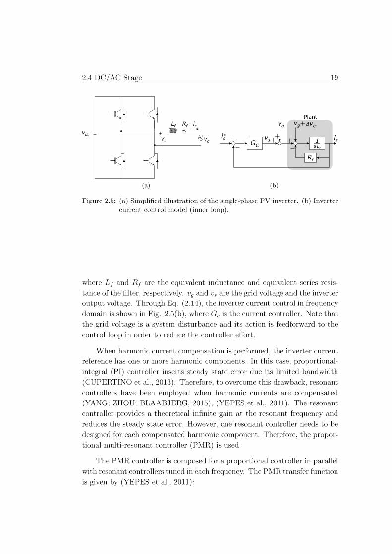
2.4 DC/AC Stage 19
(a) (b)
Figure 2.5: (a) Simplified illustration of the single-phase PV inverter. (b) Invertercurrent control model (inner loop).
where Lf and Rf are the equivalent inductance and equivalent series resis-
tance of the filter, respectively. vg and vs are the grid voltage and the inverter
output voltage. Through Eq. (2.14), the inverter current control in frequency
domain is shown in Fig. 2.5(b), where Gc is the current controller. Note that
the grid voltage is a system disturbance and its action is feedforward to the
control loop in order to reduce the controller effort.
When harmonic current compensation is performed, the inverter current
reference has one or more harmonic components. In this case, proportional-
integral (PI) controller inserts steady state error due its limited bandwidth
(CUPERTINO et al., 2013). Therefore, to overcome this drawback, resonant
controllers have been employed when harmonic currents are compensated
(YANG; ZHOU; BLAABJERG, 2015), (YEPES et al., 2011). The resonant
controller provides a theoretical infinite gain at the resonant frequency and
reduces the steady state error. However, one resonant controller needs to be
designed for each compensated harmonic component. Therefore, the propor-
tional multi-resonant controller (PMR) is used.
The PMR controller is composed for a proportional controller in parallel
with resonant controllers tuned in each frequency. The PMR transfer function
is given by (YEPES et al., 2011):

20 2 Single-Phase PV System with Ancillary Services
GC(s) = Kp +n∑h=1
Kih
Rh(s)︷ ︸︸ ︷s
s2 + ω2h
, (2.15)
where Kp is the proportional gain, h is the harmonic order (h = 1, 2, 3..., n),
ωh are resonant frequencies and Kih are the resonant gains for each harmonic
frequency. The PMR controller has high gains at its resonant frequencies.
Thereby, the term Rh(s) is responsible for tracking the current component at
each ωh frequency. The block diagram representation of the PMR is shown
in Fig. 2.6(a).
For high values of Kih, its effect on the stability can be neglected (YEPES
et al., 2011). This value can be tuned to achieve the best compromise between
selective filtering and dynamic response. On the other hand, Kp has a strong
effect on the fast transient response through bandwidth regulation, impact-
ing on the selective filtering. For high Kp values, the switching harmonics
interfere in the current control dynamic. For this reason, it is important to
ensure that the open-loop crossover frequency is lower than a decade below
the switching frequency. Therefore, the maximum acceptable Kp is given by
(YEPES et al., 2011):
KP =Rf
(1− ρ−1)√
2
√2 + 2ρ−2 − (1 +
√5)ρ−1, (2.16)
where ρ = eRfTs
Lf , Ts is the sampling period. The Bode diagram of the open-
loop with PMR controller is shown in Fig. 2.6(b). Note the high gains
imposed by the resonant controllers.
For discretization of the PMR controller, the Tustin method with pre-
warping is recommended for Rh(s). This technique avoids the shift of the
resonant frequencies in the z domain. Thus, Rh(z) is given by (YEPES et
al., 2010):
Rh(z) =sin(ωhTs)
2ωh
1− z−2
1− 2z−1cos(ωhTs) + z−2. (2.17)
It is worth emphasizing that this type of discretization requires a consid-
erable computational effort due to the presence of trigonometric functions.
2.4 DC/AC Stage 21
Simpler strategies may be used. However, deviations in resonances may occur
depending on the sampling frequency and the resonance frequencies (YEPES
et al., 2010).
(a) (b)
Figure 2.6: (a) Block diagram representation of the proportional multi-resonant(PMR) controller. (b) Bode diagram of the open-loop with the PMRcontroller.
The main goal of a closed-loop control is to reject disturbances, making
the control robust during variations in the plant. For this reason, the dynamic
stiffness (inverse of the output impedance) is applied to the inner loop control
strategy in order to verify the disturbances rejection of the system (RYAN;
BRUMSICKLE; LORENZ, 1997). Considering the disturbance ∆vg in the
grid voltage shown in Fig. 2.5(b), the output dynamic stiffness is found as:
∆vgis
= −[Lfs+Rf +Gc]. (2.18)
Therefore, the dynamic stiffness of this system is defined as the mag-
nitude of grid voltage disturbance in each frequency that causes an unit
deviation in the inverter output current. Fig. 2.7 shows the graph of the
dynamic stiffness for the designed control system. Eight resonant controllers
are considered, one tuned at fundamental frequency and seven tuned at the
odd harmonics until the 15th harmonic order. Note that, the resonant con-
trollers insert high dynamic stiffness at each resonance frequency. Note that,
the L filter effect provides high dynamic stiffness for higher frequencies.
22 2 Single-Phase PV System with Ancillary Services
Figure 2.7: Dynamic stiffness of the inverter inner loop control (∆vgis
).
2.4.2 Outer Loop Control: DC-Link Voltage Control
The outer loop is responsible for controlling the DC-link voltage. The
method based on v2dc control is employed (YAZDANI; IRAVANI, 2010).
The stored energy W in the DC-link capacitor can be expressed as:
W =1
2Cdcv
2dc, (2.19)
where Cdc is the capacitance of the DC-link capacitor. The capacitor’s in-
stantaneous power (PC) is equal to the time derivative of the stored energy,
as given by:
Pc(t) =dW
dt=
1
2Cdc
dy(t)
dt, (2.20)
where y(t) = v2dc. Thus, Eq.(2.19) can be replaced in Eq. (2.20) and expressed
in the frequency domain by:
Pc(s) = Ppv(s)− P ∗(s) =1
2CdcsY (s). (2.21)
where Ppv is the generated PV power and P ∗ is the PV inverter reference

2.4 DC/AC Stage 23
power to be injected in the PCC. Isolating Y (s) in Eq. (2.21), the following
relation is obtained:
Y (s) = 2Ppv(s)− P ∗(s)
Cdcs. (2.22)
The closed-loop block diagram is shown in Fig. 2.8. Note that, the Ppvis calculated and added to the control to reduce the controller efforts. In
such conditions, considering that the inner loop is fast enough and the PI
transfer function PI = Kpsv + Kisv/s, the closed-loop transfer function can
be represented as:
Y (s)
Y ∗(s)=
Kpsvs+Kisv12Cdcs2 +Kpsvs+Kisv
. (2.23)
Figure 2.8: Model of the DC-link control through v2dc based method.
Therefore, the poles are allocated in the frequencies f1sv and f2sv , in
which the first one is limited to one tenth below the bandwidth of the inner
loop and the second frequency limited to one tenth below the f1sv . Therefore,
applying Vieta’s formulas in the denominator of Eq. (2.23), the PI gains can
described by:
Kpsv = πCdc(f1sv + f2sv),
Kisv = 2π2Cdcf1svf2sv .
(2.24)

24 2 Single-Phase PV System with Ancillary Services
2.5 DC/AC Stage Control Strategy
Until now, the inner and outer-loops modeling were presented. In this
section, the presented models are combined to perform the DC/AC stage con-
trol strategy, including ancillary services such as reactive power injection and
harmonic current compensation. The inverter control strategy is composed
of an outer loop, designed to control the DC-link voltage and the reactive
power injection to the PCC. The inner loop is designed to control the inverter
current. This control strategy is shown in Fig. 2.9.
It is used the second order generalized integrator (SOGI) structure to
obtain the αβ components of the grid voltage at the fundamental frequency,
equivalent signals to the stationary reference frame (CIOBOTARU; TEODOR-
ESCU; BLAABJERG, 2006). This structure is important in distorted grid
voltage conditions. With the active power (P ∗) provided by the dc-link volt-
age control loop and the reactive power reference (Q∗F ), the currents i∗α and
i∗β can be found using PQ-theory given by (YANG, 2014):
i∗α =2
v2α + v2
β
(vαP∗ + vβQ
∗F ) (2.25)
where vα and vβ are the grid voltage at fundamental frequency in the sta-
tionary reference frame calculated by the second order generalized integrator
(SOGI) structure (CIOBOTARU; TEODORESCU; BLAABJERG, 2006).
The steady state error (∆Q) between the reactive power set-point (Q∗) and
the reactive power injected by the PV inverter is added to the control.
The reactive power set-point can be provided to perform some ancillary
service related to reactive power. For example, if the power factor correction
is performed, the load reactive power is measured and added to the control
as Q∗.
The harmonic current iL is detected in the load current (iLoad) and it
is added to the inverter control loop for harmonic current compensation.
This current and the fundamental current component (i∗α), calculated by the
outer-loop, are processed by the inverter current limitation techniques in or-
der to verify if the harmonic current compensation can be partial or total. It
is worth to highlight that iL inserts several frequency components in the in-
verter current reference i∗sα, which hinders the use of the PI controller. Thus,
2.5 DC/AC Stage Control Strategy 25
Harmonic
CompensationCurrent Control
Reactive Power
InjectionDC-link Control
v
2
2
Q
PI
PWM
vdc*
vpv
P*
iα
iL~
isα*
is vg
vdc
*
SOGIv α β,g
QΔ
LPFQ*
Gc
Detector
iLoad
Current
Limitation
ipv
* F
eq. (2.25)
Figure 2.9: DC/AC stage control strategy for single-phase photovoltaic inverterwith harmonic current compensation and reactive power injection ca-pabilities.
the inverter current control is performed by proportional multi-resonant con-
trollers (PMR) adjusted in each harmonic frequency to be compensated.
In the next chapters, it will be proposed two techniques to limit the peak
value of the inverter current in order to perform partial harmonic current
compensation and, next, an harmonic current detection method for selective
harmonic current compensation.
Chapter 3
Selective Harmonic Current
Compensation Strategy
In this chapter, a method for selective harmonic current compensation is
presented. The method is based on SOGI-PLL structure to detect some har-
monic current components. This method allows to compensate the harmon-
ics selectively and to adaptively tune the resonant controllers. In addition, a
complete analysis of the SOGI-PLL structure is developed in this chapter.
Many issues need to be addressed in order to use photovoltaic inverter
to compensate harmonic currents. The first one is the harmonic current
detection method. The detection methods used in harmonic compensation
can be categorized in the time and frequency-domain methods.
Different strategies have been proposed in the time domain. In Paredes et
al. (2011) and Bonaldo, Paredes and Pomilio (2016) is used the conservative
power theory for current decomposition in three orthogonal components, the
active, reactive and residual current component. In Akagi, Kanazawa and
Nabae (1984) and Watanabe, Akagi and Aredes (2008) it is used the in-
stantaneous power theory to separate the current in average and oscillating
components. Tummuru, Mishra and Srinivas (2014) use the instantaneous
symmetrical components theory for extracting the current references.
The methods cited above are widely used but they detect all the har-
monic components. As previously mentioned, total harmonic compensation
may not be possible for photovoltaic systems at certain periods of the day
and may overload the PV inverter. For this reason, there are strategies for

27
selective detection of harmonics. Rodriguez et al. (2011) propose a multires-
onant frequency locked loop (FLL) based on SOGI to detect the harmonic
components selectively. However, only one FLL is used in order to detect
the fundamental frequency component, and for detecting the other harmon-
ics this frequency is multiplied by the respective harmonic order. Also, this
information is used to tune the SOGIs structures. Therefore, this structure is
not adaptive, the harmonic components to be compensated are pre-defined.
There are detection methods in frequency domain such as discrete Fourier
transform (DFT) (MCGRATH; HOLMES; GALLOWAY, 2005), (GONZA-
LEZ; GARCIA-RETEGUI; BENEDETTI, 2007) and the fast Fourier trans-
form (ASIMINOAEI; BLAABJERG; HANSEN, 2005). The disadvantage of
these strategies is that the settling times are limited to the windowing time
period, generally one fundamental period. In addition, the requirement for
this strategy is that the harmonic should be constant during the windowing
interval (ASIMINOAEI; BLAABJERG; HANSEN, 2005).
Most of these methods mentioned above were developed and adapted
to be used in active filters, which are designed to perform only the grid har-
monic compensation. For this reason, this work introduces a harmonic detec-
tor algorithm able to detect the harmonic current selectively and adaptively
applied in PV systems, where there are several functions being performed in
some moments there is no current margin to compensate all the harmonic
current components. Therefore, the goal of this strategy is compensate as
much harmonic components as possible, respecting the physical limits of the
PV inverter.
This work proposes a harmonic current detection method based on sec-
ond order generalized integrator (SOGI) associated with the syncronous ref-
erence frame-phase-locked loop (SRF-PLL) (XAVIER et al., 2017). Gener-
ally, this structure is used as grid synchronization method for power con-
verters. The SRF-PLL structure for single-phase systems is shown in Fig.
3.1 (KAURA; BLASKO, 1997), (TEODORESCU; LISERRE; RODRIGUEZ,
2011). A quadrature signal generator provides a stationary reference frame
and then the αβ → dq transformation is used to convert the reference frame
of the input voltage from αβ to dq. The angle of the input signal is estimated
by this closed-loop structure that cancels the quadrature axis voltage and the
direct axis component aligns with the voltage space vector.
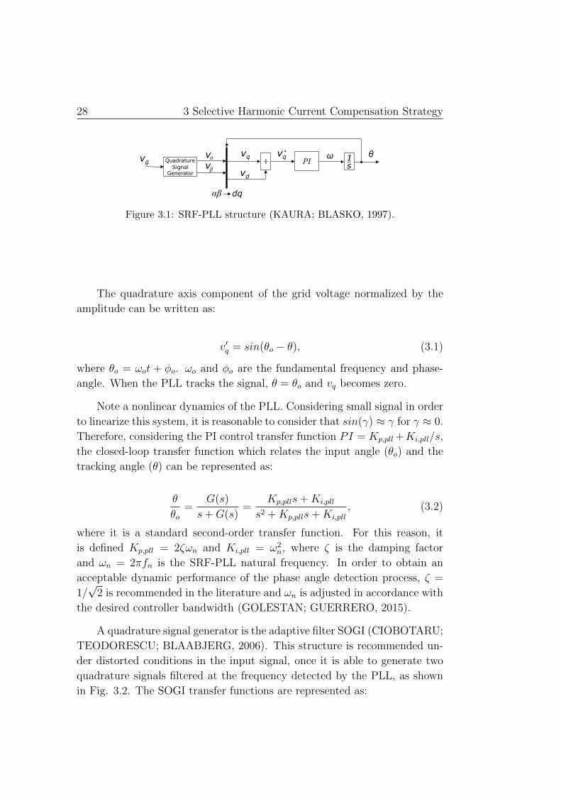
28 3 Selective Harmonic Current Compensation Strategy
Figure 3.1: SRF-PLL structure (KAURA; BLASKO, 1997).
The quadrature axis component of the grid voltage normalized by the
amplitude can be written as:
v′q = sin(θo − θ), (3.1)
where θo = ωot + φo. ωo and φo are the fundamental frequency and phase-
angle. When the PLL tracks the signal, θ = θo and vq becomes zero.
Note a nonlinear dynamics of the PLL. Considering small signal in order
to linearize this system, it is reasonable to consider that sin(γ) ≈ γ for γ ≈ 0.
Therefore, considering the PI control transfer function PI = Kp,pll +Ki,pll/s,
the closed-loop transfer function which relates the input angle (θo) and the
tracking angle (θ) can be represented as:
θ
θo=
G(s)
s+G(s)=
Kp,plls+Ki,pll
s2 +Kp,plls+Ki,pll
, (3.2)
where it is a standard second-order transfer function. For this reason, it
is defined Kp,pll = 2ζωn and Ki,pll = ω2n, where ζ is the damping factor
and ωn = 2πfn is the SRF-PLL natural frequency. In order to obtain an
acceptable dynamic performance of the phase angle detection process, ζ =
1/√
2 is recommended in the literature and ωn is adjusted in accordance with
the desired controller bandwidth (GOLESTAN; GUERRERO, 2015).
A quadrature signal generator is the adaptive filter SOGI (CIOBOTARU;
TEODORESCU; BLAABJERG, 2006). This structure is recommended un-
der distorted conditions in the input signal, once it is able to generate two
quadrature signals filtered at the frequency detected by the PLL, as shown
in Fig. 3.2. The SOGI transfer functions are represented as:

29
Figure 3.2: Complete structure of the SOGI-PLL.
Hα =vαvg
=kωs
s2 + kωs+ ω2, (3.3)
Hβ =vβvg
=kω2
s2 + kωs+ ω2, (3.4)
where k is the SOGI gain. Eqs. (3.3) and (3.4) suggest that the SOGI
structure is both bandpass and low-pass filter, respectively. An important
characteristic of the SOGI-PLL structure is that the bandwidth and cutoff
frequency only depends on the gain k. Fig. 3.3 shows the Bode diagram of
the SOGI transfer functions for three different values of k gain. Note that,
for low values of k, the bandwidth and the cut-off frequency of the SOGI are
lower.
The harmonic current detection method proposed in this work is based
on two or more cascaded SOGI-PLL, as shown in Fig. 3.4. The resonance
frequency of the SOGI-based adaptive filter (SOGI-based AF) is provided by
the SRF-PLL frequency feedback (CIOBOTARU; TEODORESCU; BLAAB-
JERG, 2006). In addition, the harmonic current detection structure consists
of two stages.
The first detector stage is responsible for detecting the parameters of
the load current fundamental component, such as its frequency (ωf = 2π60
rad/s) and amplitude. The input current of this stage is composed of the
fundamental component and several signals of different harmonic orders (h),
represented by the following equation.

30 3 Selective Harmonic Current Compensation Strategy
(a) (b)
Figure 3.3: Bode diagrams of the SOGI for tree values of the gain k(a) Hα transferfunction. (b) Hβ transfer function.
PI 1s
iq iq*
αβ dq
1s
1s
i
i
α
β
k
ωf
θf
ωf
cos
ωo
LPF
Ifid
PI 1s
ihq ihq*
αβ dq
1s
1s
α
β
k
ωh
θh
ωh
cos
ωo
LPF
Fundamental Component Detection
iLoad=Σn
h=1
cos( )Ih ωht Φh
iL
if
iL~
Harmonic Component Detection
Ihihd
= ihL=Σn
h=2
cos( )Ih ωht Φh=
ihL=Σn
h=2
cos( )Ih ωht Φhih
ih
~
~
Figure 3.4: Current harmonic detection method based on two cascaded SOGI-PLL.
iLoad =n∑h=1
Ihcos(ωht+ φh), (3.5)
where the capital latter (Ih) represents amplitude of each harmonic compo-
nent of the input current. ωh and φh is angular frequency and phase angle
of the signals. Generally, in the electrical power system the odd-numbered
31
harmonics of the fundamental frequency are more common. However, in
Eq. (3.5) the harmonic pairs are also considered, making the analysis more
generic.
In the SRF-PLL, the convention adopted in this work is to design the dq
reference frame angular position in order to make iq to zero. Therefore, the
amplitude of the current fundamental component If is equal to id filtered by
a low-pass filter (LPF). Therefore, the fundamental current component if is
detected as:
if = Ifcos(θf ), (3.6)
where θf is the fundamental component phase angle detected by the SRF-
PLL. All input current harmonic content (ihL) is determined by the difference
between the input current iL and the detected fundamental frequency if .
The second stage is similar to the previous one. However, it is responsible
for detecting the predominant harmonic current component. The harmonic
frequency ωh and amplitude Ih of the signal are detected in this stage. The
harmonic component iL is determined as:
iL = Ihcos(θh), (3.7)
where θh is the detected harmonic component phase angle. Furthermore, the
second stage is also responsible for the adaptive characteristic of the proposed
current control, i.e., the detected harmonic frequency is used to adjust the
PMR controller.
The structure presented above can be extended to detect any number of
harmonic current components present in the load current, as shown in Fig.
3.5. In this structure, n SOGI-PLLs can be connected in series.
In this work, the strategy of negative feedback is included in the har-
monic detector based on SOGI-PLL. This concept consists of subtracting
the detected harmonic components from the input signals of the previous
stages. For example, in the first stage, where the current fundamental com-
ponent is detected, all harmonic currents detected by the following stages are
removed from the input current iL. Thereby, in steady state, a cleaner signal
is provided for each detector stage, which reduces the effort detection of each

32 3 Selective Harmonic Current Compensation Strategy
stage. It is worth emphasizing that each stage provides the tuning frequency
for the proportional multi-resonant controller, making an adaptive control.
SOGI-PLL
Stage 1
iL=Σn
h=1
cos( )Ih ωht Φh==
if i2~
i(n-1)
~
in~
i2~
i(n-1)
~
in~
i(n-1)
~
in~
in~
SOGI-PLL SOGI-PLL SOGI-PLL
Stage 2 Stage (n-1) Stage n
Figure 3.5: Multi-stage harmonic detector.
In the next section, a detailed analysis is performed in order to stress the
proposed methodology. Among the analysis, it is highlighted the SOGI-PLL
tuning process, which should ensure an admissible settling time with a flexible
bandwidth to track the harmonic current component. Other important point
is the effect of the cut-off frequency of the low-pass filters (LPFs), which needs
to avoid unwanted oscillations in the detected amplitude and frequency.
3.1 Harmonic Detector Analysis
3.1.1 SOGI Gain Effect on the Harmonic Detection
For the proposed analysis, a input current iL with frequency ωh and
amplitude Ih is considered, as given by:
iL = Ihcos(ωht). (3.8)
The SRF-PLL feedback frequency is assumed to ideally track down the
frequency, i.e., the detected frequency is ωh. As mentioned previously, the
SOGI-based AF transfer functions are expressed in Eq. (3.3) and Eq. (3.4).
the signal attenuation of the SOGI increases with gain k, but with different
shapes for Hα(s) and Hβ(s). This fact can influence the harmonic signal
detection. Applying Laplace transform in Eq. (3.8), replacing it in Eqs.
3.1 Harmonic Detector Analysis 33
(3.3) and (3.4) and applying inverse Laplace transform, the time responses
of the iLα and iLβ can be obtained:
iLα(t) = Ihcos(ωht)− Ihe(−ωhkt
2)
[cosh(Aωht)−
ksin(Aωht)
2A
], (3.9)
iLβ(t) = Ihsin(ωht) +Ihe
(−ωhkt
2)sin(Aωht)
A. (3.10)
where A =√
1− k2
4. The first terms of the iLα and iLβ equations represent
the steady state and the second terms are the dynamic transient. Note two
quadrature components in steady state at the frequency ωh. This is the ideal
case, in which the SOGI can suppress any other frequency in the input signal.
However, it does not happen ideally in practice. In fact, the SOGI gain k
determines the filtering attenuation of the signal at frequency ωh.
To verify the influence of the SOGI gain on the signal filtering, the PLL
is disregarded and an input current (iL) containing a 3rd harmonic order of
amplitude 1 A and 5th harmonic order component with amplitude equal to
3 A is considered. The SOGI is tuned to filter the fifth harmonic. Fig. 3.6
shows the spectra of the iLα current for four different values of the gain k.
Note that the influence of the 3rd harmonic on the iα current decreases with
the gain value k. This is expected due to the reduction of the SOGI band-
width and cutoff frequency as already illustrated in the Fig. 3.3. This fact is
ignored in applications where the filtered signal has much larger amplitude
than the rejected signals, such as in the grid synchronization applications.
On the other hand, this work approaches a SOGI-PLL analysis for opera-
tion when the signal amplitude detected by the SOGI-PLL is similar when
compared with the rejected signal amplitude. In this operating region, un-
wanted oscillations in the detected signal are more sensitive to the SOGI-PLL
bandwidth adjustment and the low-pass filter cutoff frequency.
Analyzing Fig. 3.6, it seems obvious to choose the gain k in order to com-
pletely suppress the unwanted harmonic frequencies. In this case it seems
attractive to choose k = 0.1, but this value represents a narrow SOGI band-
width. This fact can reduce adaptability of the strategy to detect the pre-
dominant harmonic in a signal.

34 3 Selective Harmonic Current Compensation Strategy
(a)
c)(
1 3 5 7 9 11 13 15
Harmonic Order
0
1
2
3
4
Am
plit
ude [A
]
1 3 5 7 9 11 15 1
Harmonic Order
0
1
2
3
4
Am
plit
ude [A
]
1 3 5 7 9 11 13 15
Harmonic Order
0
1
2
3
4
Am
plit
ude [A
]
1 3 5 7 9 11 13 15
Harmonic Order
0
1
2
3
4
Am
plit
ude [A
]
k=0.1 k=0.8
k=10k=
(b)
(d)
Figure 3.6: Spectra of the iLα current for four different values of the gain k.(a)k = 0.1.(b) k = 0.8.(c) k =
√2.(d) k = 10
In fact, the detector has a zone that limits its adaptation and can be
explained by two factors. The first one is the SOGI bandwidth limitation
defined by the gain k. The second one is the capability of SRF-PLL to follow
the predominant harmonic component. The analysis of both phenomena are
presented in this chapter.
3.1.2 SOGI Detection Threshold
To evaluate the adaptability threshold in terms of the SOGI bandwidth,
an input current composed of a 3rd and 5th harmonic component is con-
sidered again. In addition, the complete SOGI-PLL structure is considered.
Thereby, iL is given by:
iL = I3cos(ω3t) + I5cos(ω5t), (3.11)
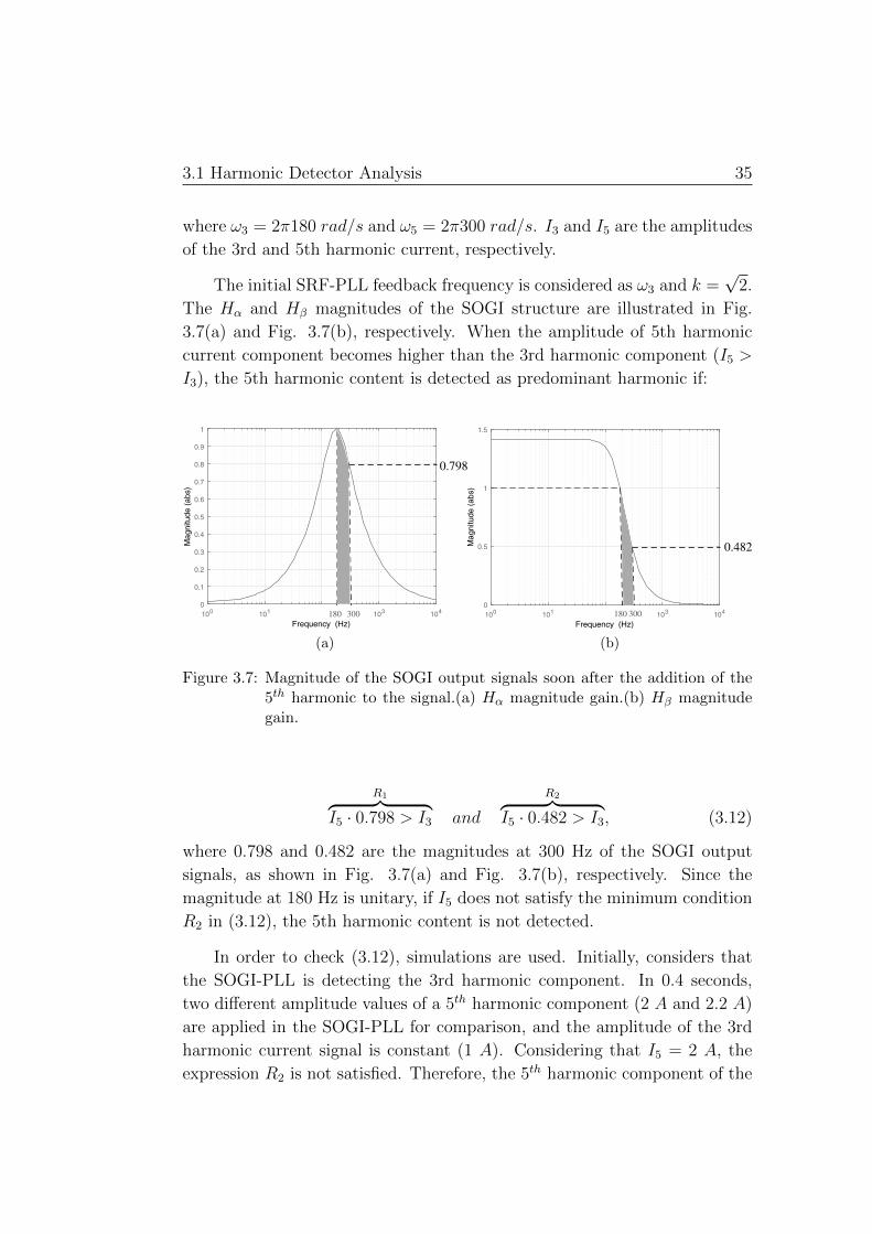
3.1 Harmonic Detector Analysis 35
where ω3 = 2π180 rad/s and ω5 = 2π300 rad/s. I3 and I5 are the amplitudes
of the 3rd and 5th harmonic current, respectively.
The initial SRF-PLL feedback frequency is considered as ω3 and k =√
2.
The Hα and Hβ magnitudes of the SOGI structure are illustrated in Fig.
3.7(a) and Fig. 3.7(b), respectively. When the amplitude of 5th harmonic
current component becomes higher than the 3rd harmonic component (I5 >
I3), the 5th harmonic content is detected as predominant harmonic if:
(a) (b)
Figure 3.7: Magnitude of the SOGI output signals soon after the addition of the5th harmonic to the signal.(a) Hα magnitude gain.(b) Hβ magnitudegain.
R1︷ ︸︸ ︷I5 · 0.798 > I3 and
R2︷ ︸︸ ︷I5 · 0.482 > I3, (3.12)
where 0.798 and 0.482 are the magnitudes at 300 Hz of the SOGI output
signals, as shown in Fig. 3.7(a) and Fig. 3.7(b), respectively. Since the
magnitude at 180 Hz is unitary, if I5 does not satisfy the minimum condition
R2 in (3.12), the 5th harmonic content is not detected.
In order to check (3.12), simulations are used. Initially, considers that
the SOGI-PLL is detecting the 3rd harmonic component. In 0.4 seconds,
two different amplitude values of a 5th harmonic component (2 A and 2.2 A)
are applied in the SOGI-PLL for comparison, and the amplitude of the 3rd
harmonic current signal is constant (1 A). Considering that I5 = 2 A, the
expression R2 is not satisfied. Therefore, the 5th harmonic component of the

36 3 Selective Harmonic Current Compensation Strategy
current is not detected, as shown in Fig. 3.8. For I5 = 2.2 A, the condition
R2 becomes true and the 5th harmonic content is detected, as shown in Fig.
3.8.
0.3 0.4 0.5 0.6 0.7 0.8
Time [s]
150
180
250
300
350
400
Fre
qu
en
cy [
Hz]
I 5 = 2 A
I 5 = 2. 2A.
Figure 3.8: 5th harmonic component detection response for two different values ofI5.
Once these analyzes have been carried out, it can be concluded that the
lower the value of k the better filtering of the signal by the SOGI in steady
state. However, the structure decreases its adaptability in a load variation
condition. Thus, there is a tradeoff between filtering capacity and system
adaptability. In this work, k =√
2 is adopted and the detection error is
minimized through the tuning of the LPF in the amplitude and frequency
detection and the PLL natural frequency design.
3.1.3 LPF Effect on the Harmonic Detection
In the proposed harmonic detector method, the LPF has an important
influence in the output characteristic, mainly when the harmonic detector in-
put iL has two or more harmonic components. Therefore, unwanted harmonic
orders must be avoided in the amplitude and frequency detection process. In
this work, the second order Butterworth low-pass filters with cut-off frequen-
cies fcf (for frequency filtering) and fca (for amplitude filtering) are used.
The input current is the same used in the SOGI gain analysis.
Fig. 3.9(a) and Fig. 3.9(b) shows the influence of three fcf and fcavalues (5 Hz, 10 Hz and 30 Hz) on the frequency and amplitude detection

3.1 Harmonic Detector Analysis 37
of the 5th harmonic component in 0.4 seconds, respectively. In steady state
conditions, the frequency ripple is 1% for fcf = 30 Hz, as depicted in Fig.
3.9(a), whereas the amplitude ripple for fca = 30 Hz is 4%, as shown in
Fig. 3.9(b). For fcf = 30 Hz, besides the direct component, there is a high
oscillation of 2nd harmonic in the detected amplitude I5, as shown in Fig.
3.9(c). Therefore, unwanted 3rd and 7th harmonic components arises in the
output current iL by the product between the 2nd harmonic oscillation and
the detected phase angle of the 5th harmonic content, which can be observed
in Fig. 3.9(d). In order to reduce the unwanted frequencies in the detected
predominant harmonic and a fast detection response for this work fca = 10
Hz and fcf = 10 Hz are adopted.
3.1.4 SRF-PLL Natural Frequency Impact on the Har-
monic Detection
The PLL natural frequency fn is adjusted in accordance with the con-
troller bandwidth. For this reason, some values of the fn are tested in order
to verify the influence of this parameter in the harmonic current detection
response.
The frequency and amplitude detection of the 5th harmonic component
for some fn values are shown in Fig. 3.10(a) and Fig. 3.10(b), respectively.
It can be observed that for fn = 10 Hz, the amplitude and frequency of
the 5th harmonic has not been detected. For fn = 100 Hz, an offset is
observed in the detected amplitude due to SRF-PLL wide bandwidth. This
wide bandwidth generates unwanted oscillations at the detected phase angle,
and thus the dq reference frame angular position is affected. The acceptable
relationship between settling time, unwanted oscillations suppressions and
lower steady-state error is found for fn = 50 Hz.
3.1.5 SRF-PLL Detection Threshold
In fact, if the input signal of SRF-PLL is composed of two harmonics
with similar amplitudes, the SRF-PLL may also limit the detector adapt-
ability and not track the predominant harmonic in the input current signal.

38 3 Selective Harmonic Current Compensation Strategy
(a) (b)
(c)
0 2 4 6 8 10
Harmonic Order
0
0.5
1
1.5
2
2.5
3
3.5
4
Am
plit
ude [A
]
(d)
Figure 3.9: Detected frequency and amplitude for three different values for bothcut-off frequencies (fcf and fca) of the LPFs, considering k =
√2.(a)
Detected frequency for three fcf values.(b) Detected amplitude forthree fca, keeping fcf = 10 Hz.(c) Detected amplitude spectrum forthree fca values, keeping fcf = 10 Hz. (d) Detected iL current spec-trum, parameters: fca = 30 Hz, fcf = 10 Hz and k =
√2
In this condition, this work defines the PLL detection threshold, which con-
sists in the minimum amplitude difference between two harmonic components
which implies in the transition of the detection between the two harmonic
components. In order to understand the SRF-PLL detection threshold, firstly
it is necessary to understand its dynamic behavior during frequency changes
(single harmonic approach).
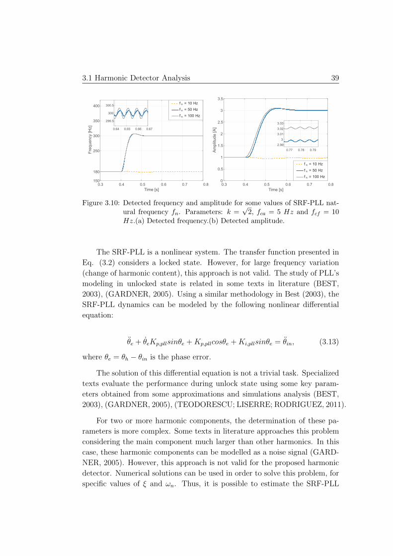
3.1 Harmonic Detector Analysis 39
Figure 3.10: Detected frequency and amplitude for some values of SRF-PLL nat-ural frequency fn. Parameters: k =
√2, fca = 5 Hz and fcf = 10
Hz.(a) Detected frequency.(b) Detected amplitude.
The SRF-PLL is a nonlinear system. The transfer function presented in
Eq. (3.2) considers a locked state. However, for large frequency variation
(change of harmonic content), this approach is not valid. The study of PLL’s
modeling in unlocked state is related in some texts in literature (BEST,
2003), (GARDNER, 2005). Using a similar methodology in Best (2003), the
SRF-PLL dynamics can be modeled by the following nonlinear differential
equation:
θe + θeKp,pllsinθe +Kp,pllcosθe +Ki,pllsinθe = θin, (3.13)
where θe = θh − θin is the phase error.
The solution of this differential equation is not a trivial task. Specialized
texts evaluate the performance during unlock state using some key param-
eters obtained from some approximations and simulations analysis (BEST,
2003), (GARDNER, 2005), (TEODORESCU; LISERRE; RODRIGUEZ, 2011).
For two or more harmonic components, the determination of these pa-
rameters is more complex. Some texts in literature approaches this problem
considering the main component much larger than other harmonics. In this
case, these harmonic components can be modelled as a noise signal (GARD-
NER, 2005). However, this approach is not valid for the proposed harmonic
detector. Numerical solutions can be used in order to solve this problem, for
specific values of ξ and ωn. Thus, it is possible to estimate the SRF-PLL

40 3 Selective Harmonic Current Compensation Strategy
detection threshold.
To illustrate this process, initially, it is used a 1 pu of 3rd harmonic signal
in the SRF-PLL input. When it reaches the steady-state, a 5th harmonic
component is added in the SRF-PLL input signal. The amplitude value of
5th harmonic component is slowly increased, in order to determine the SRF-
PLL detection threshold.
The study case results are presented in Fig. 3.11. It can be observed
that the detection threshold reduces significantly for large ξ and ωn. How-
ever, large ξ results in poor dynamic behaviour as mentioned in Teodorescu,
Liserre and Rodriguez (2011). Furthermore, large ωn increases the amplitude
offset and the estimated frequency ripple, as presented previously. For the
chosen parameters, the detection threshold is close to 1.4 pu. This value
is smaller than the threshold imposed by the SOGI bandwidth, as seen be-
fore. Therefore, for the adjustment considered in this work, the SRF-PLL
structure does not reduce the adaptability of the harmonic detector.
Figure 3.11: SRF-PLL detection threshold in function of ξ and ωn considering atransition from 3rd to 5th harmonic order.

3.2 Simulation Results 41
3.2 Simulation Results
A case study in simulation environment is used in order to validate the
harmonic current detector based on the SOGI-PLL structure for selective
harmonic current compensation. In this case study, the solar irradiance is
held constant in 300 W/m2.
The physical and control parameters of the boost converter used in this
work are shown in Table 3.1. The parameters of the PV inverter are shown
in Table 3.2.
Table 3.1: Parameters of the boost converter.
Physical Parameters ValueInductor (Lb/Rb) 0.8 mH / 0.01 mΩCapacitor (Cpv) 0.5 mFSwitching frequency (fs) 12 kHzInner-Loop Control Parameters ValueProportional gain (Kpi) 0.0155Integral gain (Kii) 0.1933Outer-Loop Control Parameters ValueProportional gain (Kpv) -0.7540Integral gain (Kiv) -132.27
Table 3.2: Parameters of the PV inverter.
LCL Parameters ValueInverter side inductor (Li/Ri) 1.5 mH / 0.03 mΩGrid side inductor (Lg/Rg) 1.5 mH / 0.03 mΩCapacitor (Cf ) 0.1 µ FDamping resistor (Rd) 4 ΩPhysical Inverter Parameters ValueInverter Rated power (Sm) 3 kVAInverter rated current (I∗m) 19.3 ADC-link Capacitor (Cdc) 3 mFSwitching frequency (fs) 12 kHzInner-Loop Control Parameters ValueProportional gain (Kp) 22.24Resonant gains (Kih) 2000Outer-Loop Control Parameters ValueProportional gain (Kp) 0.2Integral gain (Ki) 2.37

42 3 Selective Harmonic Current Compensation Strategy
The two loads shown in Fig. 3.12 are switched at the PCC at 1.4 seconds.
The maximum demand PCC current at the fundamental frequency used for
the TDD calculation is 19.3 A.
(a) (b)
Figure 3.12: Current spectra of two nonlinear loads used in the simulation casestudy. (a) Load 1. (b) Load 2.
The harmonic current detector based on the SOGI-PLL structure, pro-
posed in this work, is used to detect only two predominant harmonic com-
ponents, in terms of amplitude, in the load current. As described previously,
three stages of the detector are required, the first one responsible to detect
the fundamental current component and others two responsible to detect the
predominant harmonic contents. This harmonic detector tuning the PMR
controller frequencies adaptively. In such conditions, three resonant con-
trollers are used, one to control the fundamental component and others two
for the harmonic current component to be compensated.
Fig. 3.13 shows the amplitudes and frequencies detection of the two
predominant harmonic current of load 1 and 2. As already mentioned, the
harmonic detector is based on SOGI-PLL structure and there are three stages.
The first one responsible for detecting the fundamental component of the
load current, as shown in Fig. 3.13(a). As can be seen in Fig. 3.13(b), the
amplitude and frequency of the predominant harmonic current are detected
in stage 2. Initially, the 5th harmonic of the load 1 is detected and after
t = 1.4 seconds the 3rd is detected. Fig. 3.13(c) shows the detection of the
second predominant harmonic current by the stage 3. First, the 7th harmonic
current is detected and after t = 1.4 seconds the 5th harmonic current of the
3.2 Simulation Results 43
load 2 is detected. The three resonant controllers used in this case study are
adaptively tuned by the three detected frequencies in stage 1, 2 and 3.
The spectra of the two predominant harmonic currents detected from
load 1 and load 2 are shown in Fig. 3.14(a) and (b), respectively. The 5th
and 7th harmonic component are predominant in terms of amplitude in load
1. In load 2, the 3rd and 5th harmonic component are predominant.
The improvement of the grid current quality with selective harmonic
current compensation can be seen through the current spectra, as shown in
Fig. 3.15. This figure shows the spectra of the load, inverter and grid current
in steady state before and after the load change in 1.4 seconds. Before 1.4
seconds, the 5rd and 7th harmonic, presented in the current of the load 1,
are totally provided by the inverter, as shown in Fig. 3.15(a). In this case,
the grid current TDD is 6.90%. It is worth highlighting that if there were
no harmonic compensation, the grid current TDD would be equal to load
current, in this case 20.36%.
After 1.4 seconds, the 3rd and 5th harmonic, presented in the current of
the load 2, are totally provided by the inverter, as shown in Fig. 3.15(b). In
this case, the grid current TDD is improved from 52.72% to 14.35%.

44 3 Selective Harmonic Current Compensation Strategy
(a) (b)
(c) (d)
(e) (f)
Figure 3.13: Detected harmonic current components of the load current using theSOGI-PLL structure. (a) Fundamental current peak detected in stage1. (b) Detected fundamental frequency.(c) Predominant harmoniccurrent peak detected in stage 2. (d) Detected frequency of the pre-dominant harmonic. (e) Current peak of the second predominantharmonic current detected in stage 3. (f) Detected frequency of thesecond predominant harmonic.

3.2 Simulation Results 45
~
(a)
~
(b)
Figure 3.14: Detected current spectrum. (a) Load 1. (b) Load 2
TDD = 20.36 %
TDD = 19.45 %
TDD = 6.90 %
(a)
TDD = 14.35 %
TDD = 52.17 %
TDD = 52.72 %
(b)
Figure 3.15: Spectra of the load (iLoad), inverter (is) and grid (ig) current in steadystate before and after the load change in 1.4 seconds . (a) Before 1.4seconds. (b) After 1.4 seconds
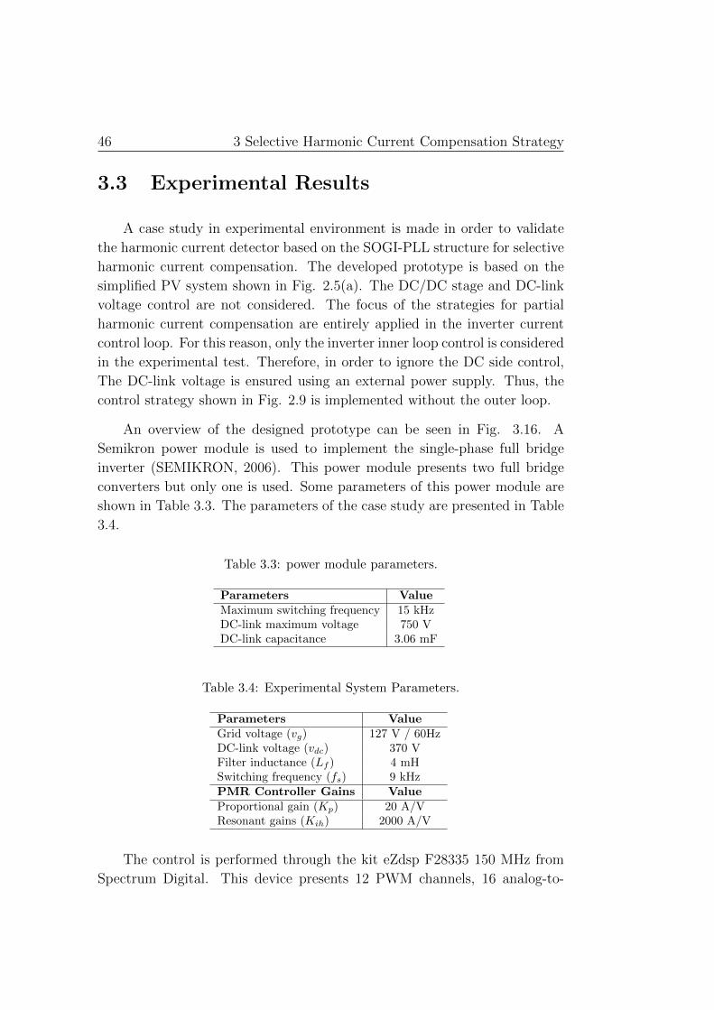
46 3 Selective Harmonic Current Compensation Strategy
3.3 Experimental Results
A case study in experimental environment is made in order to validate
the harmonic current detector based on the SOGI-PLL structure for selective
harmonic current compensation. The developed prototype is based on the
simplified PV system shown in Fig. 2.5(a). The DC/DC stage and DC-link
voltage control are not considered. The focus of the strategies for partial
harmonic current compensation are entirely applied in the inverter current
control loop. For this reason, only the inverter inner loop control is considered
in the experimental test. Therefore, in order to ignore the DC side control,
The DC-link voltage is ensured using an external power supply. Thus, the
control strategy shown in Fig. 2.9 is implemented without the outer loop.
An overview of the designed prototype can be seen in Fig. 3.16. A
Semikron power module is used to implement the single-phase full bridge
inverter (SEMIKRON, 2006). This power module presents two full bridge
converters but only one is used. Some parameters of this power module are
shown in Table 3.3. The parameters of the case study are presented in Table
3.4.
Table 3.3: power module parameters.
Parameters ValueMaximum switching frequency 15 kHzDC-link maximum voltage 750 VDC-link capacitance 3.06 mF
Table 3.4: Experimental System Parameters.
Parameters ValueGrid voltage (vg) 127 V / 60HzDC-link voltage (vdc) 370 VFilter inductance (Lf ) 4 mHSwitching frequency (fs) 9 kHzPMR Controller Gains ValueProportional gain (Kp) 20 A/VResonant gains (Kih) 2000 A/V
The control is performed through the kit eZdsp F28335 150 MHz from
Spectrum Digital. This device presents 12 PWM channels, 16 analog-to-

3.3 Experimental Results 47
(a) (b)
Figure 3.16: Setup of the designed prototype. (a) Setup overview: 1- Power mod-ule. 2- Control circuit. 3- Conditioning and control boards. 4- Mi-crocomputer. (b) Conditioning and control boards.
digital converter of 12 bit and 512 KB of FLASH memory. The signal con-
ditioning system can be seen in Fig. 3.16.
A nonlinear load based on diode rectifier was designed with variable
harmonic current content. The schematic of this load is shown in Fig. 3.17.
This load is started in three-phase mode, thus contactors 2 and 1 are closed.
A resistor RPC is used to pre-charge the capacitor bank. A timer sets a
time for this pre-charge by closing the contactor 3 in order to bypass the
resistor RPC . Once this is done, the load current can be varied between three-
phase and two-phase through the contactor 2. Thus, a single-phase inverter
connected in any phase P , E or T experiences a change in the harmonic
content of the current. The setup overview and inside view of this nonlinear
load are shown in Fig. 3.18. The current spectrum of load 1 is shown in Fig.
3.19(a). In load 1, the 5th and 7th harmonic components are predominant in
term of amplitude. Fig. 3.19(b) shows the current spectrum of load 2, which
the 3rd and 5th harmonic are predominant. Initially, load 1 is connected to

48 3 Selective Harmonic Current Compensation Strategy
the PCC.
P
E
T
Contactor 1 Contactor 2 Contactor 3
C R
RPC
PV Inverter
Figure 3.17: Schematic of the designed nonlinear load.
(a) (b)
Figure 3.18: Designed nonlinear load. (a) Setup overview. (b) Setup inside view.
0 1 3 5 7 9 11 13 15 17 19 21 23 25
Harmonic Order
0
1
2
3
4
5
6
7
8
9
i L [
A]
(a)
0 1 3 5 7 9 11 13 15 17 19 21 23 25
Harmonic Order
0
2
4
6
8
10
12
14
i L [
A]
(b)
Figure 3.19: Current spectra of two nonlinear loads used in this experimental casestudy. (a) Load 1. (b) Load 2.
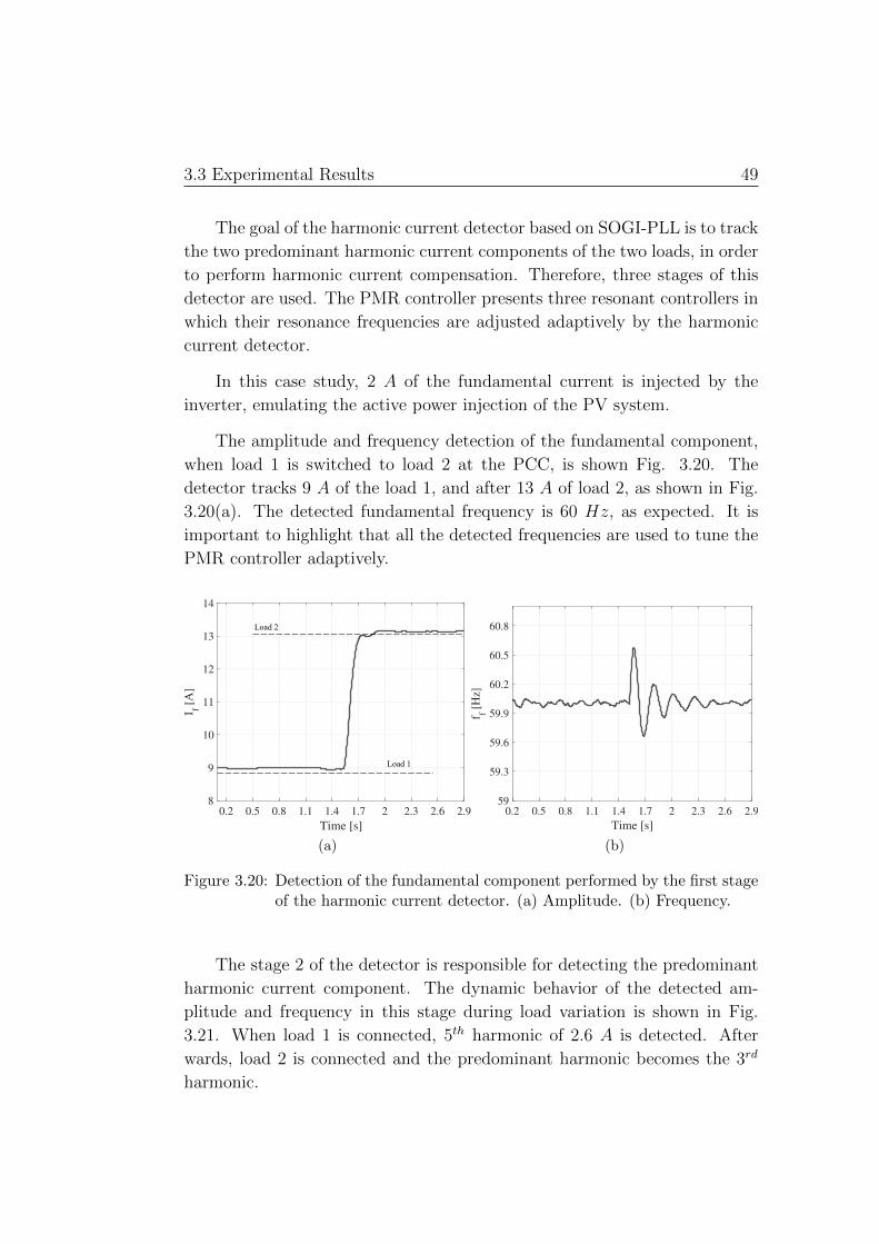
3.3 Experimental Results 49
The goal of the harmonic current detector based on SOGI-PLL is to track
the two predominant harmonic current components of the two loads, in order
to perform harmonic current compensation. Therefore, three stages of this
detector are used. The PMR controller presents three resonant controllers in
which their resonance frequencies are adjusted adaptively by the harmonic
current detector.
In this case study, 2 A of the fundamental current is injected by the
inverter, emulating the active power injection of the PV system.
The amplitude and frequency detection of the fundamental component,
when load 1 is switched to load 2 at the PCC, is shown Fig. 3.20. The
detector tracks 9 A of the load 1, and after 13 A of load 2, as shown in Fig.
3.20(a). The detected fundamental frequency is 60 Hz, as expected. It is
important to highlight that all the detected frequencies are used to tune the
PMR controller adaptively.
Load 2
Load 1
(a) (b)
Figure 3.20: Detection of the fundamental component performed by the first stageof the harmonic current detector. (a) Amplitude. (b) Frequency.
The stage 2 of the detector is responsible for detecting the predominant
harmonic current component. The dynamic behavior of the detected am-
plitude and frequency in this stage during load variation is shown in Fig.
3.21. When load 1 is connected, 5th harmonic of 2.6 A is detected. After
wards, load 2 is connected and the predominant harmonic becomes the 3rd
harmonic.
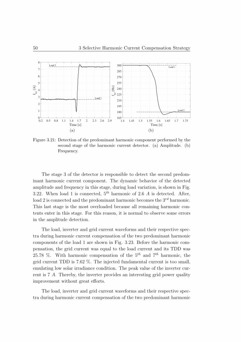
50 3 Selective Harmonic Current Compensation Strategy
Load 1
Load 2
(a)
Load 2
Load 1
(b)
Figure 3.21: Detection of the predominant harmonic component performed by thesecond stage of the harmonic current detector. (a) Amplitude. (b)Frequency.
The stage 3 of the detector is responsible to detect the second predom-
inant harmonic current component. The dynamic behavior of the detected
amplitude and frequency in this stage, during load variation, is shown in Fig.
3.22. When load 1 is connected, 5th harmonic of 2.6 A is detected. After,
load 2 is connected and the predominant harmonic becomes the 3rd harmonic.
This last stage is the most overloaded because all remaining harmonic con-
tents enter in this stage. For this reason, it is normal to observe some errors
in the amplitude detection.
The load, inverter and grid current waveforms and their respective spec-
tra during harmonic current compensation of the two predominant harmonic
components of the load 1 are shown in Fig. 3.23. Before the harmonic com-
pensation, the grid current was equal to the load current and its TDD was
25.78 %. With harmonic compensation of the 5th and 7th harmonic, the
grid current TDD is 7.62 %. The injected fundamental current is too small,
emulating low solar irradiance condition. The peak value of the inverter cur-
rent is 7 A. Thereby, the inverter provides an interesting grid power quality
improvement without great efforts.
The load, inverter and grid current waveforms and their respective spec-
tra during harmonic current compensation of the two predominant harmonic
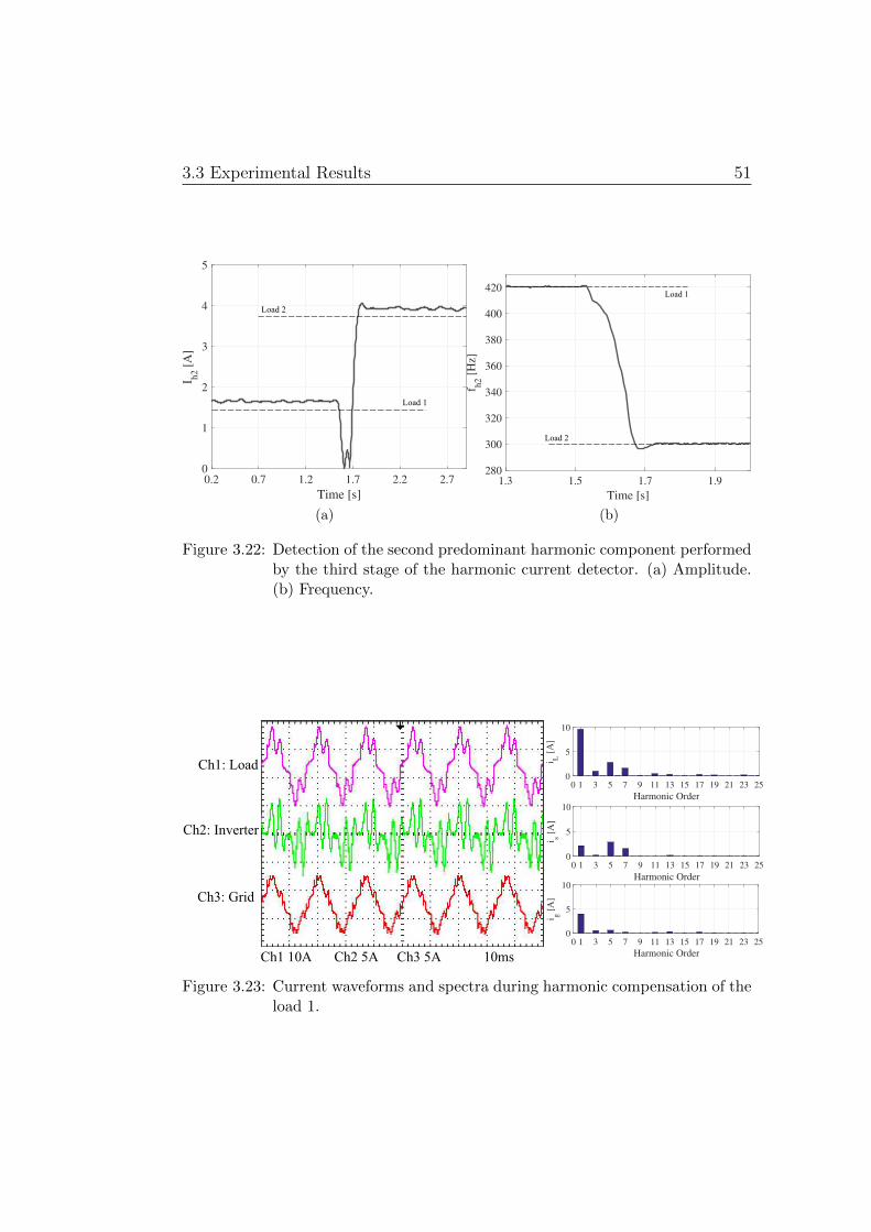
3.3 Experimental Results 51
Load 2
Load 1
(a)
Load 2
Load 1
(b)
Figure 3.22: Detection of the second predominant harmonic component performedby the third stage of the harmonic current detector. (a) Amplitude.(b) Frequency.
Ch1: Load
Ch2: Inverter
Ch3: Grid
Ch1 10A Ch2 5A Ch3 5A 10ms
Figure 3.23: Current waveforms and spectra during harmonic compensation of theload 1.
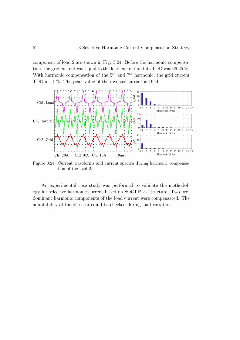
52 3 Selective Harmonic Current Compensation Strategy
component of load 2 are shown in Fig. 3.24. Before the harmonic compensa-
tion, the grid current was equal to the load current and its TDD was 66.25 %.
With harmonic compensation of the 5th and 7th harmonic, the grid current
TDD is 11 %. The peak value of the inverter current is 16 A.
Ch1: Load
Ch2: Inverter
Ch3: Grid
Ch1 20A Ch2 10A Ch3 10A 10ms
Figure 3.24: Current waveforms and current spectra during harmonic compensa-tion of the load 2.
An experimental case study was performed to validate the methodol-
ogy for selective harmonic current based on SOGI-PLL structure. Two pre-
dominant harmonic components of the load current were compensated. The
adaptability of the detector could be checked during load variation.

Chapter 4
Partial Harmonic Current
Compensation Strategy
To avoid inverter damages and to preserve its lifetime, the inverter rated
current can not be exceeded. Thereby, techniques for PV inverter current
limitation are required during ancillary services support. The critical point
is when harmonic current compensation is involved. In this condition, there
are multiple frequencies in the current signal and analytical expressions for
inverter current limitation are complex.
Some works in the literature have been introducing techniques to limit
the inverter current reference under harmonic compensation conditions. In
(GAJANAYAKE et al., 2009) a current limiting algorithm is employed based
on PI controller. A moving window RMS calculator is used to determine the
RMS value of the current and it is compared with the maximum current limit
of the inverter. The generated error signal is the input of a PI controller to
reduce the harmonic current injection. However, limiting the RMS current
value when there are multiple frequencies in the signal is not effective since
the current peak can be much larger than the RMS value, exposing the PV
inverter electronic switches to high current levels.
Therefore, this work proposes techniques to limit the peak value of the
inverter current for partial harmonic current compensation. These techniques
are independent of the harmonic current detection method. The first one is
based on a open-loop algorithm which monitors the peak of the inverter cur-
rent reference and reduces the detected harmonic current. Another technique
is presented based on a closed-loop with a PI controller in order to cancel

54 4 Partial Harmonic Current Compensation Strategy
the error between the peak value of the inverter current and its rated cur-
rent. The controller output reduces the detected harmonic current in order
to ensure that the inverter does not inject a peak current greater than the
maximum allowed. These strategies are detailed and compared below.
4.1 Open-Loop Technique
This work proposes an inverter current limitation technique based on
open-loop algorithm. This inverter current limitation scheme is presented in
Fig. 4.1. The load harmonic current (iL), the fundamental current reference
(i∗α) and the total the total inverter current reference (i∗st) are inputs of the
algorithm. The harmonic current limitation (HCL) algorithm determines
the contribution value of the iL and i∗α to the peak value of i∗st and then,
this algorithm calculates the factor (Kh) which determines the amount of
load harmonic current that can be injected in order to ensure that the peak
value of the inverter current reference (i∗sα) does not exceed the inverter rated
current I∗m. Fig. 4.2 shows the flowchart of the HCL algorithm and its step-
by-step operation is described below.
Figure 4.1: Inverter current limitation technique based on open-loop algorithm.
• The fundamental current reference (i∗α), the load harmonic current ref-
erence (iL) and the total inverter current reference (i∗st) are HCL algo-
rithm inputs. i∗st is found by the sum between i∗α and iL;
• At each sampling, the value of the i∗st is checked in order to obtain
the peak value of this current. If the new i∗st value is higher than its
previous one, the M variable is updated for this new value and the

4.1 Open-Loop Technique 55
Start
Inputs:
x = x + 1
x n
M
I =L
no
yes
Initial Value: x = -1, M = 0
i*α iL
~
istyes M = ist
I =α i*α
iL
~
x n
Output:
&&
0
Eq. 4.1 K = 0h K = 1h
Kh
Im Im*
yesno
Iα Im*
IL
yesno
==
M =
-1
I =m Mx=
0
yes
no
no
ist
Figure 4.2: Flowchart of the harmonic current limitation (HCL) algorithm.
contributions of i∗α and iL for this i∗st value are stored in IL and Iα,
respectively;
• After n samples, the peak value of i∗st is detected, which is referred as
Im. Furthermore, the contributions of IL and Iα for this peak value
are detected. The number of samples n is chosen in order to obtain a
fundamental frequency cycle;
• The peak value (Im) of i∗st is compared to inverter rated current I∗m. If
Im is less than I∗m, there is current margin for total harmonic compen-
sation, i.e., Kh = 1. However, if Im is greater than I∗m, the inverter
cannot perform the total harmonic compensation;

56 4 Partial Harmonic Current Compensation Strategy
• If Iα is greater than or equal to I∗m and the harmonic current contri-
bution (IL) is positive, the harmonic current compensation is disabled,
i.e., Kh = 0. Otherwise, the harmonic compensation will be partial
and determined by proportion ratio defined as:
Kh =I∗m − IαIL
. (4.1)
This equation means that the sum of Iα and of IL multiplied by the
factor Kh must be at most equal to the inverter rated current (I∗m);
• Finally, before the factor Kh acts on the load harmonic current (iL), a
low-pass filter (LPF) is used to suppress oscillations due to the abrupt
variations in the activity of the algorithm. The filter output is limited
between 0 and 1. Therefore, the harmonic current reference (i∗L) that
will be compensated can be represented as:
i∗L = Kh
iL︷ ︸︸ ︷n∑h=1
Ihcos(ωht+ φh) . (4.2)
This new value of the harmonic current reference is added to funda-
mental current component (i∗α) and the new inverter current reference
(i∗sα) is found. Note that, i∗sα will be equal to i∗st only if Kh = 1.
Fig. 4.3 illustrates an example of the application of this inverter current
limitation technique. It is possible to see the fundamental current reference
(i∗α) provided by the inverter outer-loop control, the load harmonic current
(iL), the total inverter current reference (i∗st) resulting from the sum of i∗α and
iL, the harmonic current reference (i∗L) resulting from the Kh factor action
and the inverter current reference (i∗sα) resulting from the sum of i∗α and i∗L .
In addition, the inverter rated current (I∗m) is set to 19.3 A.
Fig. 4.3(a) shows the input currents of the HCL algorithm. The funda-
mental current contribution (Iα) to the peak value of i∗st is 14.5 A. On the
other hand, the harmonic current contribution (IL) to the peak value of i∗stis 12 A. Therefore, the peak value (Im) of i∗st is 26.5 A. Note that it exceeds
the inverter rated current. Once the priority of the system is to inject ac-
tive power, i∗st peak value can only be reduced by reducing iL contribution.
Thereby, through (4.1), it is calculated the amount of contribution iL can
provide to the peak of i∗st. Therefore, Fig 4.3(b) shows that the contribution

4.1 Open-Loop Technique 57
of iL is reduced by the Kh factor for 40 %, which results the i∗L with contri-
bution of 4.8 A. Thus, the peak value of i∗sα is 19.3 A, which is equal to the
inverter rated current.
(a)
(b)
Figure 4.3: Details of waveforms of the currents during harmonic current compen-sation. (a) Total inverter current reference (i∗st), i.e, without Kh factoraction. (b) Inverter current reference (i∗sα), i.e, with Kh factor action.

58 4 Partial Harmonic Current Compensation Strategy
4.2 Closed-Loop Technique
Another technique proposed in this work to perform partial harmonic
current compensation is based on the PI controller action. Therefore, a
closed-loop control is designed to calculate the Kh factor used to adjust the
harmonic current reference. This closed-loop control is illustrated in Fig. 4.4.
The inverter current reference (i∗sα) is calculated by the sum between
i∗L and the fundamental current reference i∗α calculated by the outer loop.
A current peak detector monitors the peak absolute value of this current,
which is compared with the inverter rated current (I∗m). An anti-windup PI
controller, limited between 0 and 1, computes the harmonic compensation
factor Kh that weights the load harmonic current (iL), which results in the
new harmonic current reference (i∗L) in order to cancel the error between I∗mand Im.
Part of the HCL algorithm is used to detect the peak absolute value of
i∗sα, which corresponds to Imin the flowchart shown in Fig. 4.2. For this
technique, the number of samples n, used in the algorithm, is chosen in order
to obtain a fundamental frequency half cycle. For this reason, this algorithm
inserts a delay of a fundamental half cycle in the closed-loop shown in Fig.
4.4. It is also important to highlight that the factor Kh weighs the detected
harmonic component at the same frequency as that of the peak detector
activity.
Figure 4.4: Inverter current limitation technique based on PI controller.
One important challenge of this technique is designing the PI controller
gains. In fact, the PI controller design of the PI controller deserves caution
to avoid instabilities. For such, it is used part of the first technique concept
previously approached. The peak value (Im) of the inverter current reference

4.2 Closed-Loop Technique 59
can be determined as:
Im = KhIL + Iα, (4.3)
It is assumed that IL is constant and Iα is a system disturbance. These
two quantities can be found by the HCL algorithm. This is a reasonable
approximation due to the intermittent characteristic of the photovoltaic en-
ergy generation, i.e., variations in PV power generation are greater than a
considerable load harmonic current variation during the day. Thereby, the
closed-loop control modeling can be developed, as shown in Fig. 4.5.
Figure 4.5: Closed-loop control modeling of the current limitation technique basedon PI controller.
The terms e−sτ refer to the delays accounted for the peak detection al-
gorithm and Kh activity. These delay functions can be approximated by a
rational function using the first order Pade approximation method, as de-
scribed below:
e−sτ =1− s τ
2
1 + s τ2
. (4.4)
Therefore, the main goal of this closed-loop control is to reject the Iαdisturbance due to variation in the PV power generation. The transfer func-
tion which relates the peak value of the inverter current reference (Im) and
the system disturbance (Iα), making the reference I∗m equal to zero, can be
expressed as:
E(s) =Im(s)
Iα(s)=
1
1 +R(s), (4.5)
where R(s) is given by:

60 4 Partial Harmonic Current Compensation Strategy
R(s) = IL(kps+ ki)(τs− 2)2
s(τs+ 2)2, (4.6)
where Kp,sat and Ki,sat are the PI controller gains. These gains are designed
in order to achieve the better disturbance rejection performance. For this
purpose, the step response analysis of the E(s) transfer function is a good
alternative to determine the appropriate kp and ki values. The peak value
Im is detected every half cycle of the fundamental frequency of 60 Hz. Then,
τ = 1/120 seconds. Fig. 4.6 shows the step response of the E(s) transfer
function for Kp,sat = 0.08, Ki,sat = 5 and IL = 5 A. As observed, the closed-
loop rejects the step disturbance, which makes Im(∞) ≈ 0.
Figure 4.6: Disturbance rejection analysis through the step response of the E(s)transfer function.
A comparison between these two techniques for inverter current limi-
tation and the model of the closed-loop based method is performed in a
simulation environment, considering the permissible inverter rated current
(I∗m) equal to 20 A. A variable fundamental current component is injected,
whose amplitude changes from 20 A to 15 A, in steps of 1 A. In addition, a
5th harmonic current is injected with IL = 5 A. The cut-off frequency of the
low-pass filter present in the open-loop technique is 15 Hz. The computed Kh
is shown in Fig. 4.7(a). As observed, the transient response of the closed-loop
technique and the model present similar dynamics. The noticeable difference
is due to the Pade approximation of the time delay function. The computed
Kh in steady-state, depending on the injected fundamental current, is shown
in Fig. 4.7 (b). It is possible to note the similarity between these techniques

4.3 Simulation Results 61
in steady state.
(a) (b)
Figure 4.7: Kh factor calculation comparison between the two techniques for in-verter current limitation and the model of the closed-loop technique.(a) Time response of the Kh factor. (b) Steady-state response of theKh factor in relation to the fundamental current reference injected bythe inverter.
4.3 Simulation Results
The single-phase grid-connected PV system with ancillary service capa-
bility is simulated using the MATLABR© and PLECSR© software in order to
validate the inverter current limitation techniques for partial harmonic cur-
rent compensation. In the simulation, ancillary services such as harmonic
current compensation and reactive power injection are performed. The pa-
rameters of the boost converter for the DC/DC stage and the inverter are
the same already presented in Tabele 3.1 and 3.2, respectively.
Two loads are switched at the PCC in order to analyze the behavior of the
PV system control strategy addressed in this work. The current spectrum of
the load 1 is shown in Fig. 4.8(a). Besides the fundamental component, there
are odd components multiple of the fundamental frequency, except those of
triple orders. Fig. 4.8(b) shows the current spectrum of load 2, with odd
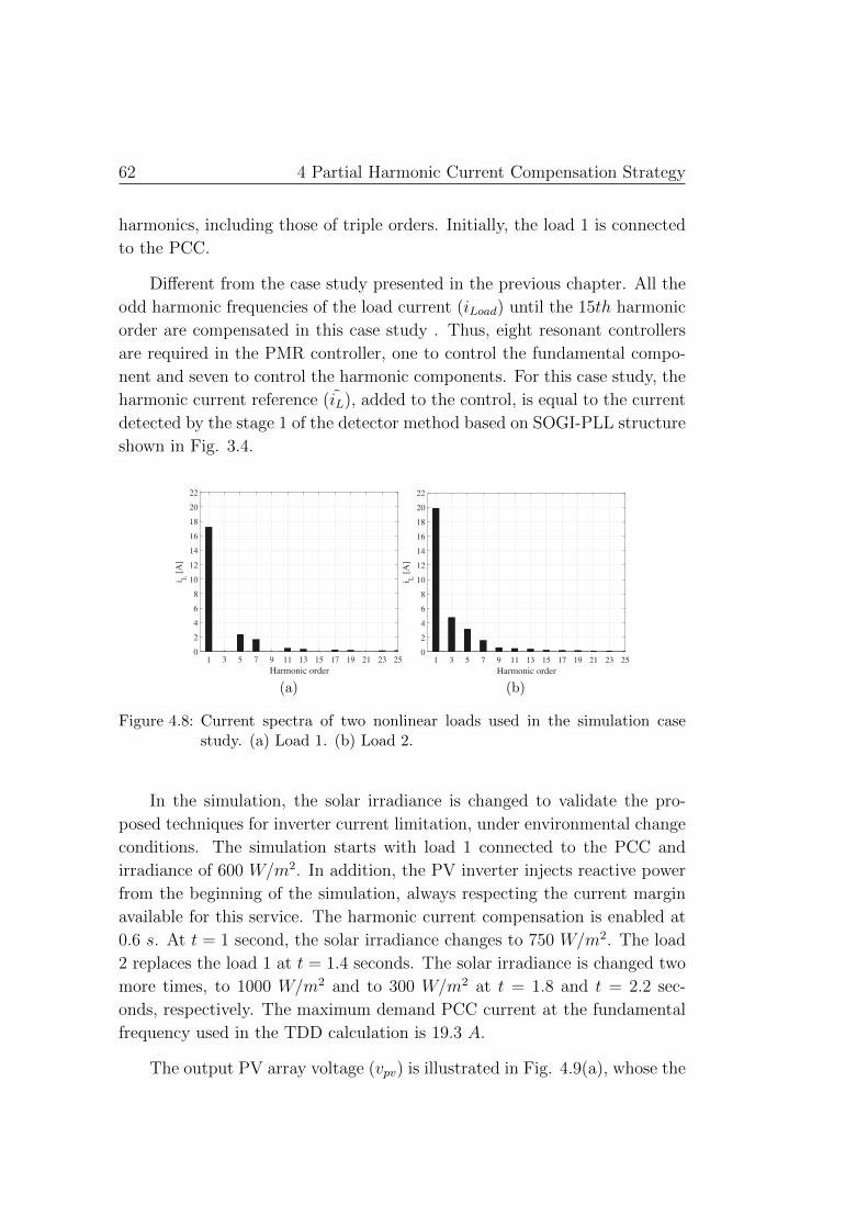
62 4 Partial Harmonic Current Compensation Strategy
harmonics, including those of triple orders. Initially, the load 1 is connected
to the PCC.
Different from the case study presented in the previous chapter. All the
odd harmonic frequencies of the load current (iLoad) until the 15th harmonic
order are compensated in this case study . Thus, eight resonant controllers
are required in the PMR controller, one to control the fundamental compo-
nent and seven to control the harmonic components. For this case study, the
harmonic current reference (iL), added to the control, is equal to the current
detected by the stage 1 of the detector method based on SOGI-PLL structure
shown in Fig. 3.4.
(a) (b)
Figure 4.8: Current spectra of two nonlinear loads used in the simulation casestudy. (a) Load 1. (b) Load 2.
In the simulation, the solar irradiance is changed to validate the pro-
posed techniques for inverter current limitation, under environmental change
conditions. The simulation starts with load 1 connected to the PCC and
irradiance of 600 W/m2. In addition, the PV inverter injects reactive power
from the beginning of the simulation, always respecting the current margin
available for this service. The harmonic current compensation is enabled at
0.6 s. At t = 1 second, the solar irradiance changes to 750 W/m2. The load
2 replaces the load 1 at t = 1.4 seconds. The solar irradiance is changed two
more times, to 1000 W/m2 and to 300 W/m2 at t = 1.8 and t = 2.2 sec-
onds, respectively. The maximum demand PCC current at the fundamental
frequency used in the TDD calculation is 19.3 A.
The output PV array voltage (vpv) is illustrated in Fig. 4.9(a), whose the

4.3 Simulation Results 63
reference voltage (v∗pv) is calculated by the MPPT algorithm. When the solar
irradiance is 1000 W/m2, vpv corresponds to the maximum power point equal
to 188 V , approximately. The boost converter inductor current is shown in
Fig. 4.9(b). The DC-link voltage is controlled in 390 V, as shown in Fig.
4.9(c). The reactive power injection starts at the beginning of the simulation
and the harmonic current compensation (HCC) is enabled at t = 0.6 seconds.
0.3 0.6 1 1.4 1.8 2.2 2.6
Time [s]
180
182
184
186
188
190
192
194
vpv [
V]
vpv
v*
pv
(a)
0.3 0.6 1 1.4 1.8 2.2 2.6
Time [s]
4
6
8
10
12
14
16
18
20
i Lb [
A]
iL
iL
*
(b)
0.3 0.6 1 1.4 1.8 2.2 2.6
Time[s]
386
388
390
392
394
396
vdc [
V]
vdc
vdc
*
(c)
Figure 4.9: Voltage and current dynamics of the PV system DC-side. (a) OutputPV array voltage (vpv). (b) Inductor current of the boost converter.(c) Dc-link voltage vdc.
The active (P ) and reactive (Q) power dynamics are shown in Fig. 4.10.
At t = 1.8 seconds, the PV system provides all active power to the the load,
as shown in Fig. 4.10(a). At this moment, there is no inverter power margin

64 4 Partial Harmonic Current Compensation Strategy
for reactive power injection, as shown in Fig. 4.10(b). At other times, the
inverter operates below its nominal power capacity, allowing it to inject all
reactive power required by the load.
(a) (b)
Figure 4.10: Dynamic of the active power (P) and reactive power (Q) flow on thesystem. (a) Active power. (b) Reactive power.
The detected harmonic current is analyzed by the inverter current limita-
tion techniques in order to determine if the harmonic current compensation
will be partial or total. Fig. 4.11 shows the harmonic compensation fac-
tor Kh calculated for both techniques addressed in this work, the open-loop
based method and closed-loop based method. It is possible to observe the
similarity between the two techniques in steady-state. When the harmonic
current compensation (HCC) is enabled at t = 0.6 seconds, the PV inverter
has current margin to compensate all harmonic current (Kh = 1). Due to
increased solar irradiance at t = 1 second, the factor Kh is approximately
0.80. Therefore, 80 % of the load harmonic current is compensated. At
t = 1.4 seconds, the PV inverter has current margin to compensate only 37
% of the harmonic current of the load 2. At t = 1.8 seconds, the harmonic
compensation is null (Kh = 0), under such condition, the PV inverter in-
jects the nominal active power. After t = 2.2 seconds, the harmonic current
compensation is total (Kh = 1).
Fig. 4.12 shows the inverter current waveform details during transient

4.3 Simulation Results 65
Figure 4.11: Compensation factor Kh using two techniques for inverter currentlimitation.
responses. At t = 0.6 seconds, the current waveform becomes more distorted
once the harmonic current compensation starts and Kh = 1. At t = 1.8
seconds, there are no harmonic components in the inverter current because
harmonic current compensation is not feasible, once the inverter injects the
nominal active. It is possible to observe that the inverter current does not
exceed the inverter rated current (I∗m) in steady-state due to factor Kh ac-
tivity.
The improvement in grid current quality with HCC is better noticed
through the total demand distortion (TDD) index, as shown in Table 4.1.
This table presents the inverter and grid current TDD in each time interval.
At the beginning, the harmonic current compensation is disabled and the
grid current TDD is 15.43 %, while the inverter injects only the fundamental
current component and thus the inverter current TDD is 1.64 %. At t = 0.6
seconds, the HCC starts and the grid current TDD becomes 3.87 %. The
worst case is between t = 1.8 and t = 2.2 seconds, when the harmonic current
compensation is disabled by the factor Kh. In this case, the grid current TDD
is 30.97 %.

66 4 Partial Harmonic Current Compensation Strategy
(a) (b)
(c) (d)
(e)
Figure 4.12: Inverter current waveform details during transient responses.(a) Tran-sient response at 1 s. (b) Transient response at t = 0.6 seconds. (b)Transient response at t = 1 second. (c) Transient response at t = 1.4seconds. (d) Transient response at t = 1.8 seconds. (e) Transientresponse at t = 2.2 seconds.
In order to demonstrate that the inverter current is bounded by its rated
value after the factor Kh action, the space phasor of the grid current is
emulated for single-phase system with and without the inverter limitation

4.3 Simulation Results 67
Table 4.1: Total demand distortion of the currents.
Time interval [s] is TDD [%] ig TDD [%]0 < t < 0.6 1.64 15.430.6 < t < 1.0 15.67 3.871.0 < t < 1.4 12.33 4.741.4 < t < 1.8 10.79 20.511.8 < t < 2.2 2.43 30.972.2 < t < 2.6 32.00 3.95
technique, as shown in Fig. 4.13. For this purpose, the current quadrature
component is obtained by delaying the current by 90o. Firstly, the space
phasor of the inverter current (is) is outside the circumference delimiting
the inverter rated current (I∗m), as shown in Fig. 4.13(a). This fact demon-
strates that the PV inverter compensates the harmonic current outside its
current margin. Due to Kh activity, the inverter current is placed within the
maximum limit, as shown in Fig. 4.13(b).
(a) (b)
Figure 4.13: Inverter current space phasor. (a) Without harmonic current limita-tion technique. (b) With harmonic current limitation technique.
A simulation case study was performed in order to validate the techniques
for partial harmonic current compensation proposed in this work. It can be
seen that even by injecting active and reactive power most of the time, the
PV inverter can help to reduce harmonic distortions in the grid current in
several moments and always respecting its current capacity.

68 4 Partial Harmonic Current Compensation Strategy
4.4 Experimental Results
A case study in experimental environment is shown in order to validate
the techniques for partial harmonic current compensation proposed in this
work. The experimental prototype of this case study is the same described
in 3.3.
In order to test these techniques under high levels of harmonic distor-
tions in the inverter current, all multiple odd harmonics of the fundamental
frequency until the 15th harmonic order are compensated. The load current
in this case study is held constant and its spectrum is shown in Fig. 3.19(b).
The case study starts when the inverter injects no fundamental current
(if = 0) and when the harmonic current compensation (HCC) is enabled.
Next, the amplitude of the fundamental current component injected by the
inverter is increased by 6 A every 1.5 seconds. Both the inverter rated current
(I∗m) and the maximum demand PCC current at the fundamental frequency
used in the TDD calculation is set to 18 A.
Fig. 4.14 shows the harmonic compensation factor in experimental envi-
ronment for both techniques addressed in this work. At the beginning of the
experiment the PV inverter has current margin to compensate all harmonic
current, i.e., Kh = 1. Due to the increase in the injected fundamental cur-
rent at t = 1.5 seconds to 6 A, the factor Kh is around 0.8, approximately.
Therefore, partial harmonic current compensation is performed from this in-
stant. At 3 < t < 4.5 seconds, the injected fundamental current is increased
again to 12 A and 18 A, respectively. The factor Kh decreases to around 0.4
and zero, respectively. Therefore, PV inverter ceases the harmonic current
compensation.
Fig. 4.15 shows current waveforms and spectra of the load, inverter and
grid during harmonic compensation with inverter current limitation tech-
nique based on the open-loop technique. At the beginning, the harmonic
compensation is total (Kh = 1) and no fundamental current is injected, which
simulates the low solar irradiance condition and no reactive power injection
service. Therefore, Fig. 4.15(a) shows high grid current quality. Almost all
load harmonic currents are supplied by the PV inverter and the grid current
is very close to a sinusoidal signal. The grid current TDD is 3.82 %. Note
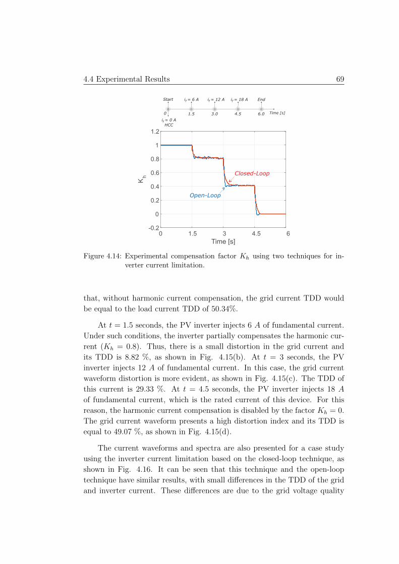
4.4 Experimental Results 69
Figure 4.14: Experimental compensation factor Kh using two techniques for in-verter current limitation.
that, without harmonic current compensation, the grid current TDD would
be equal to the load current TDD of 50.34%.
At t = 1.5 seconds, the PV inverter injects 6 A of fundamental current.
Under such conditions, the inverter partially compensates the harmonic cur-
rent (Kh = 0.8). Thus, there is a small distortion in the grid current and
its TDD is 8.82 %, as shown in Fig. 4.15(b). At t = 3 seconds, the PV
inverter injects 12 A of fundamental current. In this case, the grid current
waveform distortion is more evident, as shown in Fig. 4.15(c). The TDD of
this current is 29.33 %. At t = 4.5 seconds, the PV inverter injects 18 A
of fundamental current, which is the rated current of this device. For this
reason, the harmonic current compensation is disabled by the factor Kh = 0.
The grid current waveform presents a high distortion index and its TDD is
equal to 49.07 %, as shown in Fig. 4.15(d).
The current waveforms and spectra are also presented for a case study
using the inverter current limitation based on the closed-loop technique, as
shown in Fig. 4.16. It can be seen that this technique and the open-loop
technique have similar results, with small differences in the TDD of the grid
and inverter current. These differences are due to the grid voltage quality

70 4 Partial Harmonic Current Compensation Strategy
variation between the tests, which slightly changes the load harmonic current
content.
In relation to the computational burden, the closed-loop technique for
inverter current limitation presents an execution time of 2.68 µs to calculate
and update the factor Kh. The open-loop technique is executed in 4.24 µs
by the digital signal processor to calculate and update the factor Kh. This
execution time is accomplished when the relation shown in (4.1) is required,
which may occur at the end of each fundamental frequency cycle. Observed
that both techniques have a low execution time but the closed-loop technique
runs faster than the open-loop technique. The relation (4.1) is responsible
for increasing the computation burden of the open-loop technique.
An experimental case study was performed in order to validate the
methodology for harmonic current limitation based on a open-loop and a
close-loop technique. It was possible to verify the similarity of the two tech-
niques in steady state and the high quality improvement of the grid current
when the PV inverter has current margin to provide harmonic current com-
pensation. As can be seen that the inverter rated current (18 A) is never
exceed in any moment in steady state, ensuring the safe operation of this
device.
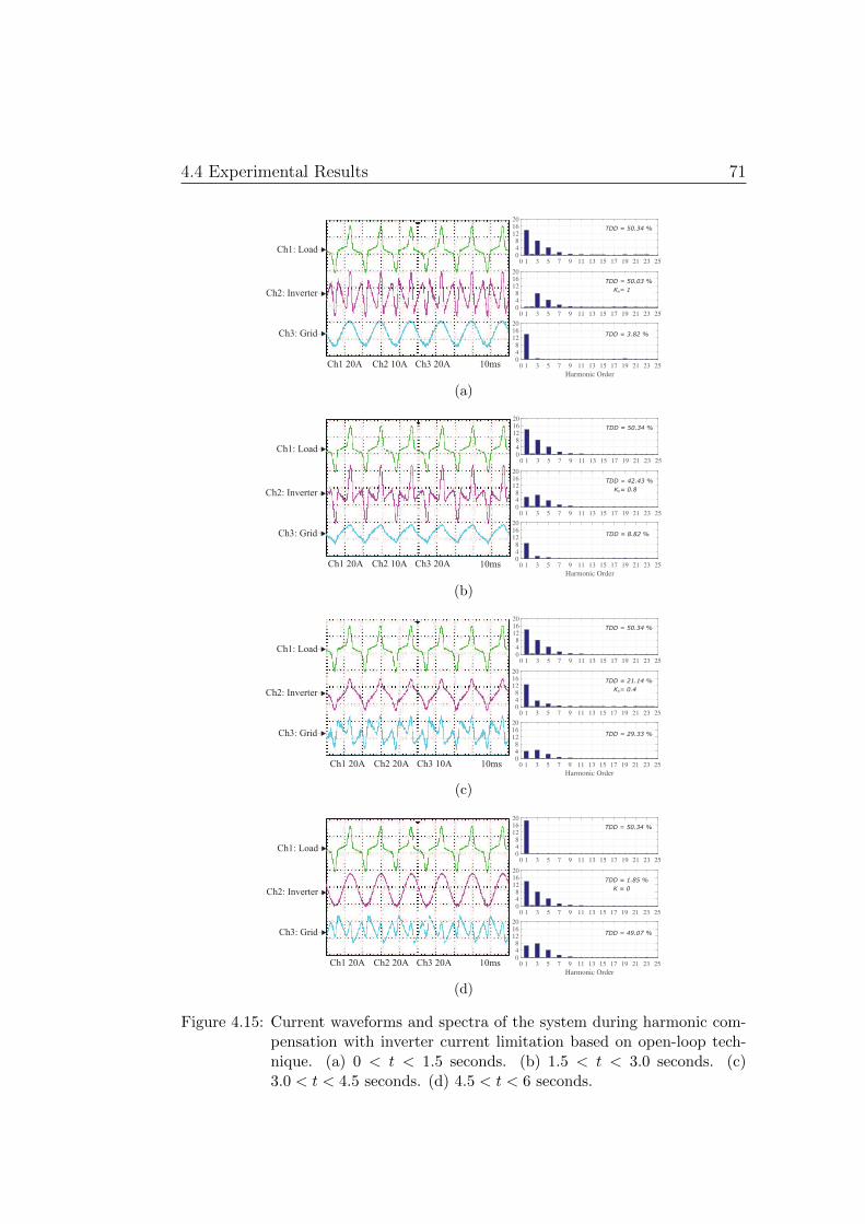
4.4 Experimental Results 71
TDD = 50.34 %
TDD = 50.03 %
K = 1h
TDD = 3.82 %
(a)
(b)
(c)
TDD = 50.34 %
TDD = 1.85 %
TDD = 49.07 %
K = 0
(d)
Figure 4.15: Current waveforms and spectra of the system during harmonic com-pensation with inverter current limitation based on open-loop tech-nique. (a) 0 < t < 1.5 seconds. (b) 1.5 < t < 3.0 seconds. (c)3.0 < t < 4.5 seconds. (d) 4.5 < t < 6 seconds.

72 4 Partial Harmonic Current Compensation Strategy
(a)
(b)
(c)
TDD = 50.34 %
TDD = 1.58 %
TDD = 48.49 %
K = 0
(d)
Figure 4.16: Current waveforms and spectra of the system during harmonic com-pensation with inverter current limitation based on closed-loop tech-nique. (a) 0 < t < 1.5 seconds. (b) 1.5 < t < 3.0 seconds. (c)3.0 < t < 4.5 seconds. (d) 4.5 < t < 6 seconds.

Chapter 5
Conclusions
This work presented a single-phase photovoltaic system connected to the
power grid with capability to perform ancillary services such as reactive power
injection and harmonic current compensation. These capabilities supports
the electrical power system under high connections of nonlinear loads and
demanding reactive power, for example.
A harmonic current detection method applied in single-phase photo-
voltaic inverters for selective harmonic current compensation was developed
in this work. This strategy was designed to extract the predominant harmon-
ics in a distorted current. In addition, the frequencies of each predominant
harmonic component were detected and then the proportional multiple res-
onant current controller can be automatically tuned for specific harmonics,
increasing the controller signal tracking capability. Analysis of the current
harmonic detector and the effect of the algorithm parameters were addressed.
Furthermore, two techniques to limit the peak value of the inverter cur-
rent for partial harmonic current compensation were proposed. One tech-
nique based on the closed-loop control and other based on open-loop method.
This work proved that the two techniques are very similar in steady state re-
sponse. The partial harmonic current have proved to be very important
ensuring that the inverter works in a safe operation mode in terms of the
current peak passing through the power switches.
Simulation and experimental results show the performance of the pro-
posed strategies and improvements in the grid current quality. The total
demand distortion (TDD) is reduced through harmonic current compensa-
tion of the nonlinear loads connected to the PCC, using the photovoltaic

74 5 Conclusions
inverter.
In such conditions, if several photovoltaic systems are already installed
into the power system, the modifications in the control strategy for partial
harmonic compensation can result in considerable improvement in the grid
power quality.
5.1 Future Works
As continuity of this work can be cited:
• It may seem consensus that inserting other services in the photovoltaic
system can reduce the lifetime of the PV inverter. Therefore, studies
about the inverter prediction lifetime during operation with ancillary
services need to carried out and compared with the lifetime in normal
operation (injecting the PV energy in the grid).
• Inverter thermal analysis with harmonic current limitation strategies
proposed here.
• Implement the strategies proposed here in a complete PV system, with
PV panels and DC/DC stage.
• Develop a strategy to limit the harmonic compensation in accordance
to the DC-link voltage.

References
ABINEE. Propostas para Insercao da Energia Solar Fotovoltaica na MatrizEletrica Brasileira. [S.l.], 2012.
AKAGI, H.; KANAZAWA, Y.; NABAE, A. Instantaneous reactivepower compensators comprising switching devices without energy storagecomponents. IEEE Transactions on Industry Applications, IA-20, n. 3, p.625–630, May 1984.
ANEEL. Resolucao Normativa n 482. Aneel, p. 9, 2012. ISSN 1098-6596.
ANEEL. Nota Tecnica n 0056/2017-SRD/ANEEL: Atualizacao dasprojecoes de consumidores residenciais e comerciais com microgeracao solarfotovoltaicos no horizonte 2017-2024. Agencia Nacional de Energia Eletrica,2017.
ANEEL. BIG - Banco de Informacoes de Geracao. 2018. <http://www2.aneel.gov.br/aplicacoes/capacidadebrasil/capacidadebrasil.cfm>.Accessed on 10/05/2018.
ASIMINOAEI, L.; BLAABJERG, F.; HANSEN, S. Evaluation of harmonicdetection methods for active power filter applications. In: Twentieth AnnualIEEE Applied Power Electronics Conference and Exposition, 2005. APEC2005. [S.l.: s.n.], 2005. v. 1, p. 635–641 Vol. 1.
BEST, R. E. Phase-locked Loops: Design, Simulation, and Applications.5th. ed. New York: McGraw-Hill Professional, 2003. 421 p.
BLAABJERG, F.; TEODORESCU, R.; LISERRE, M.; TIMBUS, A. V.Overview of control and grid synchronization for distributed powergeneration systems. IEEE Transactions on Industrial Electronics, v. 53,n. 5, p. 1398–1409, 2006.

76 References
BONALDO, J. P.; PAREDES, H. K. M.; POMILIO, J. A. Control ofSingle-Phase Power Converters Connected to Low Voltage Distorted PowerSystems with Variable Compensation Objectives. IEEE Transactions onPower Electronics, v. 31, n. 3, p. 2039–2052, 2016.
CAGNANO, A.; MEMBER, S. S.; TUGLIE, E. D.; LISERRE, M.;MASTROMAURO, R. a.; De Tuglie, E. Online Optimal Reactive PowerControl Strategy of PV Inverters. IEEE Transactions on IndustrialElectronics, v. 58, n. 10, p. 4549–4558, 2011.
CEMIG. HISTORIA DA ELETRICIDADE NO BRASIL. 2012.<http://www.cemig.com.br/pt-br/a cemig/Nossa Historia/Paginas/historia da eletricidade no brasil.aspx>. Accessed on 23/01/2018.
CIOBOTARU, M.; TEODORESCU, R.; BLAABJERG, F. A newsingle-phase PLL structure based on second order generalized integrator.PESC Record - IEEE Annual Power Electronics Specialists Conference,2006.
CUPERTINO, A. F.; CARLETTE, L. P.; PEREZ, F.; RESENDE, J. T.;SELEME, S. I.; PEREIRA, H. A. Use of control based on passivity tomitigate the harmonic distortion level of inverters. In: Innovative SmartGrid Technologies Latin America (ISGT LA), 2013 IEEE PES ConferenceOn. [S.l.: s.n.], 2013.
De la Rosa, F. C. Harmonics and Power Systems. Boca Raton: CRC PressTaylor & Francis Group, 2006.
ERICKSON, R. W.; MAKSIMOVIC, D. Fundamentals of Power Electronics.[S.l.]: Springer Science & Business Media, 2001.
GAJANAYAKE, C. J.; VILATHGAMUWA, D. M.; LOH, P. C.;TEODORESCU, R.; BLAABJERG, F. Z-source-inverter-based flexibledistributed generation system solution for grid power quality improvement.IEEE Transactions on Energy Conversion, v. 24, n. 3, p. 695–704, Sept2009.
GARDNER, F. Phaselock Techniques. 3rd. ed. Hoboken, NJ: John Wiley &Sons, 2005. 425 p.
GOLESTAN, S.; GUERRERO, J. M. Conventional synchronous referenceframe phase-locked loop is an adaptive complex filter. IEEE Transactionson Industrial Electronics, v. 62, n. 3, p. 1679–1682, 2015.
References 77
GONZALEZ, S. A.; GARCIA-RETEGUI, R.; BENEDETTI, M. Harmoniccomputation technique suitable for active power filters. IEEE Transactionson Industrial Electronics, v. 54, n. 5, p. 2791–2796, Oct 2007.
GREEN, M. A.; HISHIKAWA, Y.; DUNLOP, E. D.; LEVI, D. H.;HOHL-EBINGER, J.; HO-BAILLIE, A. W. Solar cell efficiency tables(version 51). Progress in Photovoltaics: Research and Applications, v. 26,n. 1, p. 12, 2018.
HE, J.; LI, Y. W.; MUNIR, M. S. A flexible harmonic control approachthrough voltage-controlled dg-grid interfacing converters. IEEE Transactionson Industrial Electronics, v. 59, n. 1, p. 444–455, Jan 2012.
HUSSEIN, K. H.; MUTA, I.; HOSHINO, T.; OSAKADA, M. Maximumphotovoltaic power tracking: an algorithm for rapidly changing atmosphericconditions. Generation, Transmission and Distribution, IEE Proceedings-,v. 142, n. 1, p. 59–64, jan 1995.
JOOS, G.; OOI, B. T.; MCGILLIS, D.; GALIANA, F. D.; MARCEAU, R.The potential of distributed generation to provide ancillary services. In:2000 Power Engineering Society Summer Meeting (Cat. No.00CH37134).[S.l.: s.n.], 2000. v. 3, p. 1762–1767 vol. 3.
KAURA, V.; BLASKO, V. Operation of a phase locked loop system underdistorted utility conditions. IEEE Transactions on Industry Applications,v. 33, n. 1, p. 58–63, 1997.
KEREKES, T.; TEODORESCU, R.; LISERRE, M.; KLUMPNER, C.;SUMNER, M. Evaluation of three-phase transformerless photovoltaicinverter topologies. IEEE Transactions on Power Electronics, v. 24, n. 9, p.2202–2211, 2009.
KJAER, S. B.; PEDERSEN, J. K.; BLAABJERG, F. A review ofsingle-phase grid-connected inverters for photovoltaic modules. IEEETransactions on Industry Applications, v. 41, n. 5, p. 1292–1306, 2005.
LASCU, C.; ASIMINOAEI, L.; BOLDEA, I.; BLAABJERG, F. Frequencyresponse analysis of current controllers for selective harmonic compensationin active power filters. IEEE Transactions on Industrial Electronics, v. 56,n. 2, p. 337–347, Feb 2009.
MASTROMAURO, R. A.; LISERRE, M.; KEREKES, T.; DELL’AQUILA,A. A single-phase voltage-controlled grid-connected photovoltaic system

78 References
with power quality conditioner functionality. IEEE Transactions onIndustrial Electronics, v. 56, n. 11, p. 4436–4444, 2009.
MCGRATH, B. P.; HOLMES, D. G.; GALLOWAY, J. J. H. Power converterline synchronization using a discrete fourier transform (dft) based on avariable sample rate. IEEE Transactions on Power Electronics, v. 20, n. 4,p. 877–884, July 2005.
MINAMBRES-MARCOS, V.; GUERRERO-MARTINEZ, M. A.;ROMERO-CADAVAL, E.; GONZALEZ-CASTRILLO, P. Grid-connectedphotovoltaic power plants for helping node voltage regulation. IET Renew.Power Gener., v. 9, n. 3, p. 236–244, 2015.
MORRIS, C.; PEHNT, M. Energy Transition, The German Energiewende.Energy Transition, p. 112, 2012.
PAREDES, H. K. M.; BRANDAO, D. I.; TERRAZAS, T. M.; MARAFAO,F. P. Shunt active compensation based on the Conservative Power Theorycurrent’s decomposition. In: XI Brazilian Power Electronics Conference(COBEP). [S.l.: s.n.], 2011. p. 788–794.
PAREDES, H. K. M.; MARAFAO, F. P.; BRANDAO, D. I.;COSTABEBER, A. Multi-task control strategy for grid-tied inverters basedon conservative power theory. IET Renewable Power Generation, v. 9, n. 2,p. 154–165, 2015.
PENA-ALZOLA, R.; LISERRE, M.; BLAABJERG, F.; ORDONEZ, M.;YANG, Y. LCL-filter design for robust active damping in grid-connectedconverters. IEEE Transactions on Industrial Informatics, v. 10, n. 4, p.2192–2203, 2014.
PEPERMANS, G.; DRIESEN, J.; HAESELDONCKX, D.; BELMANS, R.;D’HAESELEER, W. Distributed generation: Definition, benefits and issues.Energy Policy, v. 33, n. 6, p. 787–798, 2005.
PEREIRA, H. A.; XAVIER, L. S.; CUPERTINO, A. F.; MENDES, V. F.Single-phase multifunctional inverter with dynamic saturation schemefor partial compensation of reactive power and harmonics. In: 2015 17thEuropean Conference on Power Electronics and Applications (EPE’15ECCE-Europe). [S.l.: s.n.], 2015.
PINHO, J. T.; GALDINO, M. A. Manual de Engenharia para SistemasFotovoltaicos. CEPEL CRESESB, 2014.

References 79
PINTO, H. S.; FARIA, I. D.; BAPTISTA, R.; KASSMAYER, K.; ABBUD,A.; PINTO, V. C. A Crise Hıdrica e suas Consequencias. Nucleo de estudoe pesquisas - Senado Federal, p. 1–32, 2015.
RAUSCHENBACH, H. S. Solar Cell Array Design Handbook: ThePrinciples and Technology of Photovoltaic Energy Conversion. New York:Van Nostrand Reinhold, 1980. 549 p.
REN21. Renewables 2017: global status report. [S.l.: s.n.], 2017. v. 72.
RODRIGUEZ, P.; LUNA, A.; CANDELA, I.; MUJAL, R.; TEODORESCU,R.; BLAABJERG, F. Multiresonant frequency-locked loop for gridsynchronization of power converters under distorted grid conditions. IEEETransactions on Industrial Electronics, v. 58, n. 1, p. 127–138, Jan 2011.
RYAN, M. J.; BRUMSICKLE, W. E.; LORENZ, R. D. Control topologyoptions for single-phase ups inverters. IEEE Transactions on IndustryApplications, v. 33, n. 2, p. 493–501, Mar 1997.
SEMIKRON. Power Electronic System - SEMISTACK. 2006. <https://www.semikron.com/>. Accessed on 05/04/2018.
SERA, D.; TEODORESCU, R.; HANTSCHEL, J.; KNOLL, M. OptimizedMaximum Power Point Tracker for Fast-Changing EnvironmentalConditions. IEEE Transactions on Industrial Electronics, v. 55, n. 7, p.2629–2637, 2008.
TEODORESCU, R.; LISERRE, M.; RODRIGUEZ, P. Grid Converters forPhotovoltaic and Wind Power Systems. [S.l.]: Wiley-IEEE Press, 2011.
TUMMURU, N. R.; MISHRA, M. K.; SRINIVAS, S. Multifunctional vsccontrolled microgrid using instantaneous symmetrical components theory.IEEE Transactions on Sustainable Energy, v. 5, n. 1, p. 313–322, Jan 2014.
VILLALVA, M. G.; GAZOLI, J. R.; FILHO, E. R. Comprehensive Approachto Modeling and Simulation of Photovoltaic Arrays. Power Electronics,IEEE Transactions on, v. 24, n. 5, p. 1198–1208, 2009.
VILLALVA, M. G. G.; SIQUEIRA, T. G. G. de; RUPPERT, E. Voltageregulation of photovoltaic arrays: small-signal analysis and control design.IET Power Electronics, v. 3, n. 6, p. 869, 2010.
WATANABE, E. H.; AKAGI, H.; AREDES, M. Instantaneous p-q powertheory for compensating nonsinusoidal systems. In: 2008 International

80 References
School on Nonsinusoidal Currents and Compensation. [S.l.: s.n.], 2008. p.1–10.
XAVIER, L. S.; CUPERTINO, A. F.; PEREIRA, H. A. Adaptive saturationscheme for a multifunctional single-phase photovoltaic inverter. In:IEEE/IAS International Conference on Industry Applications. [S.l.: s.n.],2014. p. 1–8.
XAVIER, L. S.; CUPERTINO, A. F.; RESENDE, J. T. de; MENDES,V. F.; PEREIRA, H. A. Adaptive current control strategy for harmoniccompensation in single-phase solar inverters. Electric Power SystemsResearch, Elsevier B.V., v. 142, p. 84–95, 2017.
YANG, Y. Advanced Control Strategies to Enable a More Wide-ScaleAdoption of Single-Phase Photovoltaic Systems. 150 p. Tese (Doutorado) —Aalborg University, 2014.
YANG, Y.; WANG, H.; BLAABJERG, F. Reactive Power InjectionStrategies for Single-Phase Photovoltaic Systems Considering GridRequirements. IEEE Trans. Ind. Appl., v. 50, n. 6, p. 4065–4076, 2014.
YANG, Y.; ZHOU, K.; BLAABJERG, F. Frequency adaptability ofharmonics controllers for grid-interfaced converters. International Journalof Control, v. 90, n. 1, p. 3–14, 2015.
YAZDANI, A.; IRAVANI, R. Voltage-Sourced Converters in Power Systems:Modeling, Control, and Applications. [S.l.]: Wiley-IEEE Press, 2010. 541 p.
YEPES, A. G.; FREIJEDO, F. D.; DOVAL-GANDOY, J.; LOPEZ, O.;MALVAR, J.; FERNANDEZ-COMESANA, P. Effects of DiscretizationMethods on the Performance of Resonant Controllers. IEEE Trans. PowerElectron., v. 25, n. 7, p. 1692–1712, 2010.
YEPES, A. G.; FREIJEDO, F. D.; LOPEZ, O.; DOVAL-GANDOY, J.Analysis and Design of Resonant Current Controllers for Voltage-SourceConverters by Means of Nyquist Diagrams and Sensitivity Function. IEEETransactions on Industrial Electronics, v. 58, n. 11, p. 5231–5250, 2011.